

Submitted:
29 August 2026
Posted:
31 August 2026
You are already at the latest version
Abstract
Spiking Neural Networks (SNNs) promise ultra-low-power, event-driven computation; however, current efforts to integrate self-attention into spiking transformers predominantly rely on global attention mechanisms, introducing growing token complexity when scaling and diluting discriminative feature representations. We introduce Spike-Driven Neighborhood Attention (SDNA) over the full k×k neighbors window in two forms, Pairwise SDNA, which gates each query–neighbor interaction before aggregating, and Linear SDNA, which exploits the absence of a softmax in spiking attention to pool the key–value interaction over the window and gate it once, evaluating the spiking gate per position rather than per query–neighbor pair. Both operators are placed in a fully local hierarchical backbone that increases the receptive field without any global attention layer. Across static and neuromorphic benchmarks the two operators are competitive with global spike-driven transformers at comparable or lower parameter counts. On CIFAR-10 Pairwise SDNA reaches 97.24% and on N-Caltech101 Linear SDNA reaches 89.65%, each the highest among the compared spike-driven transformers and obtained with fewer parameters. These results indicate that dense global attention is not necessary for these tasks and that a full local neighborhood, with the gate reordered, is sufficient.
Keywords:
spiking neural networks
; spiking transformers
; spike-driven neighborhood attention
1. Introduction
Spiking Neural Networks have emerged as biologically inspired alternatives to conventional Artificial Neural Networks (ANNs), offering low-power, event-driven computation [1,2,3,4,5] with a natural match to neuromorphic hardware [6]. Grounded in the dynamics of biological neurons [7], they have been combined with deep architectures to exploit spatial and temporal structure and applied across a range of tasks [8,9,10,11]. Convolutional spiking models, however, struggle to capture long-range dependencies without substantial memory and energy overhead [12,13]. Transformers, developed for language [14,15,16] and extended to vision [17,18,19,20], address this through attention, though at a significant compute and memory cost [21,22]. Spiking transformers were introduced to combine the low-energy, event-driven nature of SNNs with the representational power of attention [23,24,25,26].
Most spiking transformers adopt global attention, in which every token interacts with every other. Beyond its quadratic cost, dense global interaction can dilute the response in the task-relevant regions that carry the discriminative signal, which has motivated a shift toward local attention in the non-spiking setting [27,28,29]. In the spiking domain this direction remains largely unexplored. A recent local spiking attention mechanism [30] restricts attention through sparse dilated sampling, which lowers cost but discards most of the neighborhood and can lose the fine local structure a full window would retain.
The Spike-Driven Transformer (SDT) [24] already exploits one consequence of removing the softmax. Without a normalization over the attended set, the key–value interaction can be aggregated first and the query applied afterwards, which yields a linear-cost global operator [24]. This reordering has so far been used only for global attention, where a single aggregate is shared by all queries. In the local setting the same freedom takes a different and unexploited form, because each query attends to its own window and no single aggregate can be shared.
We bring this reordering to local attention. We first construct the direct spiking realisation of neighborhood attention, Pairwise SDNA, in which each query is scored against every key in its neighbors window, the score is gated by a spiking neuron, and the gated values are summed. Because the spiking gate is a pointwise nonlinearity rather than a softmax over the window, the gating and the summation can be exchanged. This gives our second operator, Linear SDNA, which pools the key–value interaction over the window and gates it once, applying the query to the pooled result. Both operators attend over the full neighborhood rather than a sparse sampled subset of it, so the fine local structure a window carries is preserved. We place them in a hierarchical spiking backbone that applies the same local operator at every stage and reduces spatial resolution across stages, so a single local primitive composes into a global receptive field using dilation without any global attention layer.
Our contributions are summarized as follows: First, we introduce two spike-driven neighborhood attention operators over the full neighbors window, Pairwise SDNA and Linear SDNA, and show that the absence of a softmax in spiking neighborhood attention allows the gating and the window aggregation to be reordered without approximation. Second, we show that the reordered operator, Linear SDNA, evaluates the spiking gate once per position rather than once per query–neighbor pair, and we characterise what this placement of the gate costs in selectivity and saves in computation. Third, we build a fully local hierarchical spiking transformer in which the same neighborhood operator is applied at every stage, so a global receptive field is reached by composition rather than by any global attention layer. Finally, to demonstrate the effectiveness of our approach, we perform extensive experiments on static and neuromorphic benchmarks, including CIFAR-10, CIFAR-100, N-Caltech101, DVS128-Gesture and ImageNet, together with ablations that isolate the effect of gate placement, gate calibration, and membrane time constant.
2. Related Works
2.1. Spiking Transformers
Transformer architectures have been adapted to SNNs to give them content-dependent, adaptive feature aggregation, which convolution’s fixed kernels cannot provide. The difficulty is that self-attention is also the most expensive component to make spike-driven, cost grows with the number of tokens, and softmax normalization has no spike-form equivalent. The work below can be read as successive attempts to retain the benefit of attention while reducing what it costs, first by simplifying the computation, then by changing the abstraction, and finally by restricting its spatial scope. Spikformer [23] introduced the first fully spiking transformer, replacing softmax attention with spiking self-attention (SSA) that operates directly on binary spike tensors. Removing the softmax leaves an attention map computed from spike-form queries and keys, but the operator remains global, every token attends to every other, at a cost quadratic in the number of tokens.
SDT [24] simplified the arithmetic of that operator. Since the product of two spike tensors reduces to a logical AND, SDT replaces the matrix multiplications of SSA with element-wise Hadamard products and a column-wise sum, so that attention performs only mask-and-accumulate operations and is genuinely spike-driven on neuromorphic hardware. The scope stays global, but the cost becomes linear in the token count, single key–value aggregate is formed once and shared across all queries.
QKFormer [31] changed the abstraction of attention rather than its arithmetic. Its Q-K token attention computes an importance score from the query and key alone, with no value-side interaction and no pairwise attention map, giving linear complexity in the token count. This operator is used in the early stages, where tokens are many and channels few, while the later stages revert to spiking self-attention. The whole is arranged as a hierarchical backbone whose token count decreases and embedding dimension increases from stage to stage, placing the cheapest attention where the tokens are most numerous.
These operators restrict what attention computes while leaving its scope global. LSFormer [30] instead restricts where attention looks, introducing a local structure-aware spiking self-attention that samples keys and values along horizontal and vertical dilated strips and assigns different dilation rates to different channel groups to recover multi-scale receptive fields. Its efficiency comes from attending to fewer sampled positions rather than from the structure of the local window itself.
Wherever these operators aggregate over a set of query–key interactions, whether globally as in SSA and SDT or locally as in LSFormer, the spiking nonlinearity is applied to each interaction before that aggregation. The ordering is inherited from softmax attention, where normalizing over the attended set requires the nonlinearity to act on the assembled scores. A spiking gate carries no such requirement. It is pointwise, and nothing binds it to the per-pair scores. Whether the gate must precede aggregation, and what is gained by moving it, is the question this work takes up.
2.2. Efficient Attention Mechanisms
Global self-attention computes an interaction between every pair of tokens, so its cost and memory grow quadratically with the sequence length. Restricting attention has therefore become the dominant route to efficiency in vision transformers. Swin [28] partitions the feature map into non-overlapping windows and computes attention within each, reducing cost to linear in the token count for a fixed window size, and recovers cross-window information by shifting the partition between consecutive blocks. Neighborhood attention [27] replaces partitioning with a sliding window that each query attends to the window of its nearest neighbors, so the windows overlap and move with the query. This preserves translation equivariant, which the shifted-partition scheme does not, requires no pixel shifts to grow the receptive field, and reduces to dot-product self-attention when the window reaches the size of the feature map. Both localise attention by restricting which keys a query may attend to, while leaving the internal structure of the operator unchanged. That internal structure is constrained by the softmax. Normalizing the attention weights over the attended set requires all query–key scores to be assembled before the weights can be formed, which fixes the order of operations to score every pair, normalize, then aggregate the values. The key–value product cannot be pooled in advance, because the normalization depends on the individual scores. Non-spiking work that reassociates the computation, as in linear attention, must therefore replace the softmax with a kernel feature map to remove this dependency.
Spiking attention removes the softmax outright [23], since it has no spike-form equivalent, and replaces it with a pointwise spiking gate. The constraint that fixes the order of operations therefore does not apply, spiking neighborhood operator may pool the key–value interaction over the window first and gate the pooled result once, with the query applied afterwards. This reordering requires no approximation and no kernel substitution; it follows from the absence of a normalization over the attended set. The present work takes up this possibility and examines what it costs and what it saves.
3. Materials and Methods
This section develops two spike-driven neighborhood-attention operators. Neighborhood attention has been brought to spiking networks before [30], though in a different architecture and a different formulation from ours. We first construct the direct spiking realization, Pairwise SDNA, which gates every query–neighbor pair (Section 3.2). We then observe that, because the spiking gate is a pointwise nonlinearity rather than a softmax over the window, the gate can be moved from before the window sum to after it. This second placement, Linear SDNA, is a reformulation the softmax-free setting permits, and it removes a factor of from the gating cost.
3.1. Preliminaries
In a spiking network, the activations passed between layers are spike events, not real numbers. Under multi-spike neurons an activation is a small non-negative integer; under binary neurons it is either 0 or 1. The energy-relevant quantity is the number of synaptic operations (SOPs), that is spike-triggered accumulations. As established in the spike-driven transformer line [24], a product of two spikes reduces to a logical AND, so the only arithmetic spike-driven layer performs is a spike-gated accumulation, in which a spike triggers one accumulation and silence triggers nothing. The data path has no multipliers and no subtractors. We treat this event-driven sparsity as the property the operator must preserve, and throughout the paper we call an operator spike-driven only when every elementary operation it performs is a spike-gated accumulation.
3.1.1. Neuron Model
The base unit is the leaky integrate-and-fire (LIF) neuron [1], written in the iterative form used for direct training. At physical time-step t, the membrane potential charges, fires, and resets according to
where is the input from the preceding layer, is the membrane potential after charging but before firing, is the potential after firing, leak term with the membrane time constant, is the threshold, is the output spike, and is the Heaviside step function. The leak carries information across time-steps. The non-leaky integrate-and-fire variant replaces (1) with , integrating the unscaled input current without decay. Equation (3) is the soft reset, which subtracts the threshold on firing and is the reset we use; a hard reset, which instead clears the potential to a fixed value, is the alternative.
We build on the integer-firing neuron of the Spike Firing Approximation (SFA) method [32]. A binary spike discards the magnitude of a neuron’s response, collapsing strong and marginal activations to the same single spike, whereas the integer code retains that magnitude and preserves the representational precision that dense inputs and attention scores depend on. At inference the integer activation is unrolled into an equivalent binary spike train over D virtual sub-steps, exactly, so the deployed network is purely binary and spike-driven. We write for this neuron applied element-wise, which is the gate used in the operators below. Static models use it at a single physical time-step, while event models use a leaky form that integrates evidence across physical time-steps with a per-dataset time constant . The integer fire function, the virtual-step construction, and the two temporal regimes are given in Appendix A.
3.1.2. Spiking Transformer Backbone
The operator sits inside a hierarchical spiking-transformer backbone. We write N for the number of spatial tokens at a stage, C for the channel count, T for the number of physical time-steps, and k for the square neighborhood kernel size, so each query attends over a window. The query, key and value spike tensors are Q, K, V; is the query at position i, and , are the key and value at a neighbor j. The set of positions in the window centered on i is . The windows may be dilated, changing the membership of but leaving the analysis below unchanged. We write ⊙ for the channel-wise Hadamard product which treats channels independently.
Restricting attention to a local window forces a choice. A neighborhood operator needs a different window sum at every position, and the only way to compute these overlapping sums with spike-gated accumulation alone is to re-accumulate each window directly, at cost per position; the kernel-independent alternative, an integral image, relies on dense subtraction and is not spike-driven. We keep the spike-drivenness and accept the cost, which is what a per-neighbor operator already pays; Appendix B gives the full argument. Our contribution, as detailed in Section 3.2, is that within this spike-driven branch, one design choice removes a factor of from both the number of spiking-gate evaluations and attention memory, at a small and measured cost in selectivity.
Once window accumulation is fixed, one decision settles the operator, namely where to place the spiking gate relative to the window sum. The gate is the nonlinearity that turns the accumulated evidence into spikes. It can act on each neighbor before the sum, or once on the pooled sum, and these two placements give the two operators below. Both sit on the same ladder, between global aggregation with one shared sum and per-neighbor gating with a decision at every neighbor. The two are instantiated by the same registered model with identical parameters; only the forward computation changes.
3.2. Spike-Driven Neighborhood Attention
We now proceed towards describing Spike-Driven Neighborhood Attention (SDNA), as illustrated in Figure 1. Pairwise SDNA is the direct spiking realization of neighborhood attention (Figure 1, top). It scores each query–neighbor pair (4), gates each score with the spiking neuron (5), and sums the gated values over the window (6):
This is the natural first construction, and it keeps per-neighbor selectivity, since it can fire on a single strong neighbor and retains which neighbor that was. It is also the operator against which the reformulation is measured below. The costs follow from Equations (4)–(6). The operator materializes per-neighbor score and attention tensors whose size grows with , it gates values (one spiking-gate evaluation for every neighbor), and its attention memory scales as .
The linear SDNA operator (Figure 1, bottom) computes the key–value coincidence once per position, pools it over the window, gates the pooled result a single time, and re-weights by the query:
The coincidence in Equation (7) is computed once per position and reused by every window that contains j. The pooling in Equation (8) is a spike-gated box-sum, the window-accumulation branch. The gate then acts once, on the pooled value. Note that the query enters after the gate, modulating the gated regional aggregate rather than a per-neighbor score. The factor keeps the gate input in a bounded band as k grows. We call this operator Linear SDNA because the spiking gate is evaluated once per position, so the number of gate evaluations is linear in the token count and independent of the window size, where the pairwise form evaluates the gate for every query–neighbor pair and scales with the window.
Because the gate is a pointwise spiking neuron rather than a softmax normalized over the window, the SN nonlinearity is not tied to the per-pair scores, and it can be applied either before or after the window sum. The two placements are therefore both admissible, but they are not equivalent. Gating each neighbor and then summing is not the same function as summing and then gating, since the gate is nonlinear. The two operators differ only in this order, and the resulting difference in what they compute is measured in the results. The order of gating and summation contrasts as
and in where the query enters, at the score or at the final product. Three cost properties follow from this one change. Linear SDNA performs times fewer spiking-gate evaluations, one per position () rather than one per neighbor (), and that count does not grow with k. Its attention-map memory is and independent of k, against for Pairwise, so the neighborhood can be widened without a memory penalty. And the key–value coincidence is computed once per position and reused by every window that contains it, rather than recomputed for each query–neighbor pair, which lowers the constant factor at the same asymptotic cost .
Sum-then-gate cannot tell which neighbor carried the evidence. It sees only the regional aggregate , where gate-then-sum makes a separate decision per neighbor. Pairwise SDNA can respond to a single discriminative neighbor and identify it. In contrast, Linear SDNA pools weak evidence into one robust quantity and gives up the per-neighbor detail.
3.2.1. Neighborhood Positional Encoding
The window in Equations (4) and (8) is symmetric and per channel, so on its own the operator cannot tell a neighbor above the query from one below it, and some form of positional information must be supplied. The standard mechanism in windowed attention is a relative position bias (RPB) [28,33], a learnable bias indexed by the query–neighbor offset and added to the score of each pair. RPB applies naturally to Pairwise SDNA, where a per-pair score exists (Equation (4)). It does not transfer to Linear SDNA. There the neighbor contributions are summed into a single aggregate before the gate acts (Equation (8)), which collapses the relative offsets that RPB indexes, so no per-pair bias can be attached. A relative-position signal could, in principle be reintroduced by weighting neighbors before pooling, but this is no longer RPB.
We therefore supply position through a Conditional Positional Encoding (CPE) [34], which both operators can use. CPE is a depthwise convolution (DWConv) per-block followed by batch normalization (BN), added residually to the spike tensor before each attention block,
Because it acts on the token map rather than on per-pair scores, CPE is independent of the operator and applies unchanged to both Pairwise and Linear SDNA. Over binary spikes, the depthwise convolution is accumulation-only, and the encoding is small. It is the architecture’s main positional signal, and Linear SDNA relies on it alone, while Pairwise SDNA could additionally use RPB.
3.2.2. Neighbor Gating
In neuromorphic datasets, the gate requires one adjustment. The input of the pooled window (Equations (4) and (8)) is the average of spike coincidences over the window, and on sparse event streams this average sits close to zero, so the gate rarely reaches its firing threshold and falls largely silent. We therefore normalize the gate input on the neuromorphic models before gating,
and the gate acts on and for the pairwise and linear models, respectively. This centers the pooled coincidence across the firing threshold and restores gate activity; its effect is analyzed in Section 4. The static models, whose dense inputs keep the gate active, gate directly and do not use this normalization.
3.3. Architecture Overview
We adopt the hierarchical spiking transformer backbone of QKFormer [31], illustrated in Figure 2, comprising a spiking patch-embedding module (SPEDS) that also performs down-sampling between stages, a sequence of stages operating at decreasing spatial resolution and increasing channel width, and a classification head that is grouped over space and time. The SPEDS modules and the membrane-shortcut residual convention are taken from that design unchanged, and we describe them only briefly in the following. The input tensor has N channels ( polarity channels for event data, for RGB static images); every tensor exchanged between components after the first SPEDS is a spike tensor, so the network is accumulate-only, and the neuron model is the one defined in Section 3.1. Our architectural contribution is not the backbone, but what fills its attention layers, described next.
QKFormer applies different attention operators at different depths, using a token-level attention (QKTA) which forms an importance mask from queries and keys alone, in the early token-rich stages, and full spiking self-attention (SSA) in the final stage. We depart from this and at all stages, including the earliest and highest-resolution, use the same local operator, the spike-driven neighborhood attention block of Section 3.2. No stage forms a global token-to-token map. This is made viable by two properties acting together. First, the SDNA operator’s cost is linear in the number of tokens and independent of the grid extent, so it stays affordable on the large early grids where a global operator would not be. Second, the hierarchy itself supplies global reach, since a fixed-size window covers a small fraction of an early, fine grid but a large fraction of a late, coarse one, so the effective receptive field grows by composition across stages rather than by any single global layer. The network is therefore uniformly local, yet globally expressive.
Every stage uses the same window, so the number of attended positions is fixed across the hierarchy, and only the dilation varies, decreasing with depth so that each stage’s effective reach stays commensurate with its grid.
Each stage is a stack of identical blocks, and each block applies three residual operations in sequence,
CPE is the depthwise convolution of Equation (11) for positioning the local windows, the SDNA operator projects the block input to spiking queries, keys and values with linear projections, restricts mixing to the dilated window around each position, and projects the result back; its interior, where the spiking gate sits relative to the window sum, is the subject of Section 3.2 and is the paper’s main contribution. The SMLP is the Spiking Multilayer Perceptron used for channel mixing in spike-driven transformers [23]; it is identical across the operator variants we compare. All three residual additions are spike-tensor additions, following the membrane-shortcut convention of the backbone rather than inserting a neuron on the shortcut path.
The remaining components (the SPEDS patch embedding and downsampling modules and the classification head) are taken from the backbone [31] and are detailed in Appendix C.
4. Results
In this section, we evaluate the two SDNA approaches on static and neuromorphic datasets including static CIFAR-10/100 [35] and ImageNet [36] datasets, as well as event-driven neuromorphic N-Caltech101 [37] and DVS128-Gesture [38] datasets.
4.1. Experimental Setup
All models share the following configuration. We train with AdamW and a cosine learning-rate schedule with linear warmup, label smoothing , and automatic mixed precision. Every stage uses a neighborhood window with per-channel attention, conditional positional encoding, and integer-firing neurons. Each model is trained with five random seeds and we report the mean and standard deviation, except on ImageNet, where results are from a single run. Table 1 lists the settings that differ between experiments.
4.2. CIFAR Results
On the static CIFAR benchmarks (Table 2), Pairwise SDNA attains the highest CIFAR-10 accuracy in the comparison at , above LSFormer [30] ( ) and QKFormer [31] (), with Linear SDNA close behind at ; both exceed all prior methods on this dataset at fewer parameters (6.76 M against 9.32M for Spikformer and 9.50 M for LSFormer). On CIFAR-100 the two operators are on par with the strongest prior methods: Pairwise SDNA reaches , within one standard deviation of STMixer ( ) and LSFormer (), and above QKFormer (81.15), while Linear SDNA reaches .
4.3. ImageNet Results
We evaluated the operators at scale on ImageNet-1K at . Beyond the common settings of Section 1, the ImageNet models use a three-stage backbone of ten blocks with a per-stage dilation of 7, 5, 4, a base learning rate of scaled to an effective batch of 512 over four GPUs, and augmentation techniques including random augmentation [43] and random erasing [44] following DeiT [45] have been used. Results are reported for a single run. Table 3 shows that both operators scale well. At the 8-384 configuration (16.6M parameters) Pairwise and Linear SDNA reach and , exceeding Spikformer and the Spike-driven Transformer at comparable size by five to seven points, and at 8-512 (29.3M) they reach and . The latter matches the strongest baseline, STAtten at , while using fewer than half its parameters (29.3M against 66.3M). Consistent with the trend on dense inputs, Pairwise SDNA slightly leads Linear SDNA on this static benchmark.
4.4. Neuromorphic Benchmarks
We compared the two SDNA operators against prior spiking transformers on the neuromorphic benchmarks in Table 4. On N-Caltech101, Linear SDNA reaches the highest accuracy in the comparison, exceeding the global-attention models SDT [24] and Spikformer [23] by and respectively, and improving on QKFormer [31] by . It also exceeds LSFormer [30], the closest local spiking-attention method, by . Pairwise SDNA is likewise competitive, above all prior methods on this dataset. On DVS128-Gesture, where accuracies are saturated near the ceiling, both operators reach on average over multiple seeds, ahead of Spikformer (), QKFormer (), and LSFormer (), and within points of SDT, which is highest at . Both operators achieve these results at fewer parameters than the compared methods.
In contrast to the static datasets where Pairwise SDNA outperforms Linear SDNA, for neuromorphic datasets, Linear outperforms Pairwise. This suggests that for sparse event streams Linear is the stronger of the two, consistent with the pooling in Linear SDNA aiding aggregation where activity is sparse and costing a little where it is dense.
4.5. Analysis and Ablations
Having established that the two operators are competitive in accuracy, we now analyze what separates them and what governs their behaviour on event data. We first isolate the cost of the reordering, measuring how the memory and throughput of the two operators scale with the neighborhood size. We then examine two factors specific to the neuromorphic setting, the membrane time constant and the calibration of the attention gate, both of which act on the same underlying quantity, the rate at which the network fires. Together, these establish where the efficiency of Linear SDNA comes from and why the event models require the choices made in Section 3.
4.5.1. Efficiency of the Reordering
Figure 3 compares the two operators directly as the neighborhood grows, with every other factor held fixed. The pair of neighbors, incurs a cost that increases with k. At the window used in our models the difference is already present, at lower memory and higher throughput, and it increases steadily as the neighborhood expands, reaching lower memory and higher throughput at . The two operators are therefore not interchangeable in cost even though they attend over the same window. The reordering that leaves accuracy essentially unchanged is what makes the larger neighborhoods affordable, since Linear SDNA sustains them at close to constant cost while Pairwise SDNA does not.
4.5.2. Batch Normalization Effect on Gate Channels
The attention gate consumes an unnormalized product of two spike quantities, and on the sparse event data this product concentrates close to zero, so the fixed firing threshold is rarely reached and the gate is largely silent. Adding a channel-wise normalization to the gate input re-expands this distribution across the threshold. Figure 4(a) shows the effect directly: without the normalization the gate barely fires in any block, and adding it lifts the gate firing rate across all three. Figure 4(b) shows the accuracy that follows, for Pairwise and for Linear. The larger gain for Linear SDNA is consistent with its stronger dependence on the gate because it applies a single gate to the pooled window rather than one gate per neighbor, a starved gate removes proportionally more of its signal.
4.5.3. Effect of the Membrane Time Constant
The leaky integer neuron used on the event benchmarks integrates over the physical time-steps with the update , where a single scalar sets the decay . Because the leak acts only across physical steps, it applies only to the event models; the static models run at a single physical step, so has no effect (Appendix A).
Table 5 sweeps homogeneously across all spiking nodes, with every other setting fixed at the reported configuration. Three observations follow. First, the optimum is consistent across all four curves, over both datasets and both operators, peaking at . That the two operators agree matters, since it means is a property of the backbone and the data rather than something re-tuned per operator, so the operator comparison is not confounded by a per-operator choice of . Second, the effect is large on N-Caltech101 and the sweep spans roughly five accuracy points, larger than the gap between the two operators. Third, the optimum is interior and the falloff is asymmetric, with accuracy degrading gently below and steeply above it.
The mechanism behind the sweep is the network’s firing rate. Training on N-Caltech101 across different , higher produces markedly lower firing and lower accuracy. As shown in the table, raising to 3 starves the gate and costs about five accuracy points. Firing rate tracks accuracy across most of the range but does not fully determine it. The highest firing model (=1.25) is not the most accurate, so more spiking is not monotonically better. The natural reading of the loss below the optimum is temporal integration. As falls, decreases and the membrane retains less history, which on event data, where the signal is spread across frames, costs more than the added drive returns.
5. Discussion
In this paper, we introduced spike-driven neighborhood attention and studied where the spiking gate should sit relative to the neighboring window. The direct form, Pairwise SDNA, gates each query–neighbor interaction before aggregating, while the reordered form, Linear SDNA, exploits the absence of a softmax in spiking attention to pool the key–value interaction first and gate it once. The central finding is that this reordering is almost free in accuracy while changing the cost of the operator. Limiting attention to a few tokens, and further reducing the gating to a single evaluation per position, does not sacrifice representational quality. Across static and neuromorphic benchmarks the two operators remain competitive with global spike-driven attention, and on N-Caltech101 and CIFAR-10 they exceed it.
A single mechanism accounts for much of what we observe, namely the rate at which the network and its attention gate fire. The membrane time constant controls this rate directly. As it increases, the network fires progressively less and activation sparsity rises, and beyond an interior optimum the model is starved of spikes and loses accuracy, so the best operating point is one of moderate rather than maximal or minimal firing. The gate calibration acts on the same quantity by a different route. Without it, the unnormalized gate input on sparse event data sits below the firing threshold, and the gate falls largely silent, and restoring its activity through normalization recovers the lost accuracy. That two independent interventions, one on the neuron time constant and one on the gate input, move accuracy through the same firing-rate channel indicates that spike availability, rather than any single architectural choice, is the binding constraint on these operators.
Our results place these operators within a line of spiking transformers that reduce the cost of attention in different ways. Spikformer [23] and the Spike-driven Transformer [24] retain full global attention, in which every token interacts with every other, while QKFormer [31] reduces this cost by forming a token-importance mask from queries and keys alone. All of these keep a global scope and our experiments can show that this scope is not required. By restricting attention to a local neighborhood, they avoid diluting the response across the entire feature map, and they remain competitive with these global models while surpassing them on N-Caltech101 and CIFAR-10, which indicates that the discriminative signal for these tasks is already present within a local window. The one prior spiking method to take a local route, LSFormer [30], reaches locality differently, sampling sparse dilated strips within a columnar backbone rather than attending over the full neighborhood in a hierarchy. Attending to the complete window, our operators match its accuracy across these benchmarks and exceed it on N-Caltech101, suggesting that the fine local structure discarded by sparse sampling carries usable discriminative information.
Two limitations qualify these results. The first concerns where the efficiency of the operators can be realized. The reduction we obtain is in the number of spiking-gate evaluations and in attention memory, quantities that fall regardless of the platform, but converting that reduction into wall-clock speed depends on the hardware. Current GPUs are optimized for large dense matrix multiplication and reward neither the accumulate-only nature of spike–spike interaction nor the fine-grained, locally windowed access pattern of neighborhood attention, so on a GPU the operation-count advantage of the local operator is not reflected in runtime. The saving is therefore best read as a property of the computation rather than a measured speed-up on general-purpose hardware.
The second limitation is one of measurement. Our strongest results are on the neuromorphic benchmarks, where the datasets are small and the test sets limited in size, so seed-to-seed variance is non-negligible and the accuracy differences between close configurations are not always individually separable. The time-constant sweep in particular was run at a single seed and used for selection rather than for statistical comparison between adjacent values, and the reported accuracies, while averaged over several seeds, carry standard deviations that overlap for the nearest competing methods on some datasets. These results should therefore be read as evidence of a consistent trend and a competitive operating point rather than of a precisely resolved ranking.
Both limitations point toward the same line of future work. A spike-driven local operator maps naturally onto hardware built for event-driven accumulation and fine-grained spatial access rather than dense matrix products, and a dedicated accelerator could exploit the sparsity and locality that a general-purpose GPU leaves unused, realizing the operation-count advantage as an end-to-end latency and energy gain. Alongside this, evaluation on larger benchmarks would tighten the variance that the small neuromorphic datasets leave in the current results.
Acknowledgments
This publication is part of the project ROBUST: Trustworthy AI-based Systems for Sustainable Growth with project number KICH3.L TP.20.006, which is (partly) financed by the Dutch Research Council (NWO), ASMPT, and the Dutch Ministry of Economic Affairs and Climate Policy (EZK) under the program LTP KIC 2020-2023. All content represents the opinion of the authors, which is not necessarily shared or endorsed by their respective employers and/or sponsors.
Appendix A. Spike Firing Approximation and Temporal Regimes
Binary firing emits at most one spike per step and cannot register how far the membrane exceeds the threshold, collapsing every activation to a single spike regardless of magnitude. The integer code of the Spike Firing Approximation (SFA) [32] preserves this magnitude and recovers representational precision, which most improves accuracy on dense inputs. During training, with the threshold set to unity, the neuron emits the integer
where confines the membrane potential U to , rounds to the nearest integer, and D is the maximum level, so a single step carries a graded value rather than one binary spike; the binary neuron is the case . At inference the same integer is realised as a sequence of D binary spikes,
so the network runs as a purely binary, spike-driven system while reproducing the integer used in training. The two are equal exactly under a soft-reset neuron at unit threshold, since a neuron given the membrane potential at the first sub-step and zero input thereafter fires once per sub-step and subtracts the threshold on firing, emitting precisely s spikes.
The model has two distinct time axes. The virtual sub-steps above encode a single integer activation and are non-leaky, which is the condition that makes the integer-to-spike equivalence exact. Separately, the physical time-steps t carry the actual input sequence, and the two data modalities differ only in how the neuron behaves along this physical axis. On static images the input is presented at a single physical step, so no membrane state is carried between steps and the integer level D alone provides the graded code. On neuromorphic data the input is a temporal sequence over several physical steps, and the membrane retains a decayed fraction of its previous state between them (Equation (1)), so the neuron integrates evidence across the event stream while still emitting an integer per step. The decay is set by a time constant , a per-dataset setting reported with the results. Because the leak acts only across physical steps, has no effect on the static models, which run at a single physical step, and it is swept only for the event models.
Appendix B. Locality, Kernel-Independence, and Spike-Drivenness
Global spike-driven attention is linear in N and spike-driven at once for a structural reason. It forms one aggregate, , and shares it across every query [24], so there is a single accumulation, nothing slides, and the cost is . Locality removes the property that makes this possible, since a neighborhood operator needs a different window sum at every position and adjacent windows overlap as they slide across the feature map.
The usual way to compute overlapping window sums cheaply is an integral image. One precomputes a prefix sum and recovers any window in constant time by inclusion–exclusion, at per position and independent of k. We do not use it. Inclusion–exclusion subtracts dense, multi-bit prefix sums at every position, and subtraction of dense values is not a spike-gated accumulation, so the kernel-independent route is not spike-driven. The remaining option is to re-accumulate each window directly, which is spike-driven but costs per position and therefore depends on the kernel size. A local aggregator thus cannot be both kernel-independent and spike-driven under the two implementations one would actually reach for. We do not claim that no algorithm can attain all three properties, only that this trade is forced in practice, and we keep spike-drivenness.
Appendix C. Inherited Backbone Components
The SPEDS module performs patch embedding, spikification, and inter-stage downsampling through a short stack of convolution, normalization and spiking-neuron units. The first SPEDS is the only place in the network that consumes real-valued input, and each subsequent SPEDS halves the spatial resolution and doubles the channel width. It uses max pooling rather than strided convolution, which on spike tensors preserves sparse activity, since a spike anywhere in the pooling footprint survives, rather than diluting it. The classification head reduces the final stage by global average pooling over space, averages over the T time-steps, and applies a single linear classifier; averaging over time after spatial pooling lets the readout integrate evidence across the temporal window, which matters on event data where individual time-steps are sparse.
References
- Maass, W. Networks of spiking neurons: The third generation of neural network models. Neural Netw. 1997, 10, 1659–1671. [Google Scholar] [CrossRef]
- Kudithipudi, D.; Schuman, C.; Vineyard, C.M.; Pandit, T.; Merkel, C.; Kubendran, R.; Aimone, J.B.; Orchard, G.; Mayr, C.; Benosman, R.; et al. Neuromorphic computing at scale. Nature 2025, 637, 801–812. [Google Scholar] [CrossRef]
- Karamimanesh, M.; Abiri, E.; Shahsavari, M.; Hassanli, K.; van Schaik, A.; Eshraghian, J. Spiking neural networks on FPGA: A survey of methodologies and recent advancements. Neural Netw. 2025, 186, 107256. [Google Scholar] [CrossRef]
- Shahsavari, M.; Thomas, D.; van Gerven, M.; Brown, A.; Luk, W. Advancements in spiking neural network communication and synchronization techniques for event-driven neuromorphic systems. Array 2023, 20, 100323. [Google Scholar] [CrossRef]
- Roy, K.; Jaiswal, A.; Panda, P. Towards spike-based machine intelligence with neuromorphic computing. Nature 2019, 575, 607–617. [Google Scholar] [CrossRef]
- Hill, A.J.; Donaldson, J.W.; Rothganger, F.H.; Vineyard, C.M.; Follett, D.R.; Follett, P.L.; Smith, M.R.; Verzi, S.J.; Severa, W.; Wang, F.; et al. A spike-timing neuromorphic architecture. In Proceedings of the 2017 IEEE International Conference on Rebooting Computing (ICRC); IEEE, 2017; pp. 1–8. [Google Scholar]
- van Gerven, M. Dynamical systems foundations for neuromorphic intelligence. Neuromorphic Comput. Eng. 2026, 6, 014022. [Google Scholar] [CrossRef]
- Tavanaei, A.; Ghodrati, M.; Kheradpisheh, S.R.; Masquelier, T.; Maida, A. Deep learning in spiking neural networks. Neural Netw. 2019, 111, 47–63. [Google Scholar] [CrossRef]
- Eshraghian, J.K.; Ward, M.; Neftci, E.O.; Wang, X.; Lenz, G.; Dwivedi, G.; Bennamoun, M.; Jeong, D.S.; Lu, W.D. Training spiking neural networks using lessons from deep learning. Proc. IEEE 2023, 111, 1016–1054. [Google Scholar] [CrossRef]
- Fatahi, M.; Shahsavari, M.; Ahmadi, M.; Ahmadi, A.; Boulet, P.; Devienne, P. Rate-coded DBN: An online strategy for spike-based deep belief networks. Biol. Inspir. Cogn. Archit. 2018, 24, 59–69. [Google Scholar] [CrossRef]
- Huebotter, J.; Lanillos, P.; van Gerven, M.; Thill, S. Spiking neural networks for continuous control via end-to-end model-based learning. Neuromorphic Comput. Eng. 2026, 6, 024004. [Google Scholar] [CrossRef]
- Hassanshahi, M.; Shahsavari, M.; van Gerven, M. Energy-efficient spiking recurrent neural network for gesture recognition on embedded GPUs. arXiv preprint 2024, arXiv:2408.12978. [Google Scholar]
- Yin, B.; Corradi, F.; Bohté, S.M. Accurate and efficient time-domain classification with adaptive spiking recurrent neural networks. Nat. Mach. Intell. 2021, 3, 905–913. [Google Scholar] [CrossRef]
- Vaswani, A.; Shazeer, N.; Parmar, N.; Uszkoreit, J.; Jones, L.; Gomez, A.N.; Kaiser, L.; Polosukhin, I. Attention is all you need. In Proceedings of the Proceedings of the 31st International Conference on Neural Information Processing Systems, Red Hook, NY, USA, 2017; NIPS’17, pp. 6000–6010. [Google Scholar]
- Devlin, J.; Chang, M.; Lee, K.; Toutanova, K. BERT: Pre-training of deep bidirectional Transformers for language understanding. In Proceedings of the North American Chapter of the Association for Computational Linguistics; Association for Computational Linguistics, 2019; pp. 4171–4186. [Google Scholar] [CrossRef]
- Zhang, H.; Shafiq, M.O. Survey of transformers and towards ensemble learning using transformers for natural language processing. J. Big Data 2024, 11, 25. [Google Scholar] [CrossRef]
- Dosovitskiy, A.; Beyer, L.; Kolesnikov, A.; Weissenborn, D.; Zhai, X.; Unterthiner, T.; Dehghani, M.; Minderer, M.; Heigold, G.; Gelly, S.; et al. An image is worth 16x16 words: Transformers for image recognition at scale. In Proceedings of the International Conference on Learning Representations, 2021. [Google Scholar]
- Li, L.H.; Yatskar, M.; Yin, D.; Hsieh, C.J.; Chang, K.W. VisualBERT: A simple and performant baseline for vision and language. arXiv preprint 2019, arXiv:1908.03557. [Google Scholar]
- Yuan, L.; Chen, Y.; Wang, T.; Yu, W.; Shi, Y.; Tay, F.E.H.; Feng, J.; Yan, S. Tokens-to-token ViT: Training vision transformers from scratch on ImageNet. In Proceedings of the Proceedings of the IEEE/CVF International Conference on Computer Vision (ICCV); IEEE, 2021; pp. 538–547. [Google Scholar]
- Carrigg, K.; van Gastel, R.; Yeghaian, M.; Dalm, S.; Boughorbel, F.; van Gerven, M. Decorrelation speeds up vision Transformers. In Proceedings of the Proceedings of the Computer Vision Conference (CVC) 2026; Volume 1, Arai, K., Lorenz, P., Eds.; Cham, 2026; pp. 284–302. [Google Scholar]
- Tay, Y.; Dehghani, M.; Bahri, D.; Metzler, D. Efficient Transformers: A survey. ACM Comput. Surv. (CSUR) 2022, 55, 1–28. [Google Scholar] [CrossRef]
- Carrigg, K.; de Vries, S.; Sadough, A.; van Gerven, M. Evolving layer-specific scalar functions for hardware-aware transformer adaptation. arXiv preprint 2026, arXiv:2605.14047. [Google Scholar]
- Zhou, Z.; Zhu, Y.; He, C.; Wang, Y.; YAN, S.; Tian, Y.; Yuan, L. Spikformer: When spiking neural network meets Transformer. In Proceedings of the The Eleventh International Conference on Learning Representations, 2023. [Google Scholar]
- Yao, M.; Hu, J.; Zhou, Z.; Yuan, L.; Tian, Y.; Xu, B.; Li, G. Spike-driven Transformer. In Proceedings of the Thirty-seventh Conference on Neural Information Processing Systems, 2023. [Google Scholar]
- Tang, X.; Chen, T.; Cheng, Q.; Shen, H.; Duan, S.; Wang, L. Spatio-temporal channel attention and membrane potential modulation for efficient spiking neural network. Eng. Appl. Artif. Intell. 2025, 148, 110131. [Google Scholar] [CrossRef]
- Zhou, S.; Yang, B.; Yuan, M.; Jiang, R.; Yan, R.; Pan, G.; Tang, H. Enhancing SNN-based spatio-temporal learning: A benchmark dataset and cross-modality attention model. Neural Netw. 2024, 180, 106677. [Google Scholar] [CrossRef]
- Hassani, A.; Walton, S.; Li, J.; Li, S.; Shi, H. Neighborhood attention transformer. In Proceedings of the Proceedings of the IEEE/CVF Conference on Computer Vision and Pattern Recognition, 2023; pp. 6185–6194. [Google Scholar]
- Liu, Z.; Lin, Y.; Cao, Y.; Hu, H.; Wei, Y.; Zhang, Z.; Lin, S.; Guo, B. Swin Transformer: Hierarchical vision transformer using shifted windows. In Proceedings of the Proceedings of the IEEE/CVF International Conference on Computer Vision, 2021; pp. 10012–10022. [Google Scholar]
- Jiao, J.; Tang, Y.M.; Lin, K.Y.; Gao, Y.; Ma, A.J.; Wang, Y.; Zheng, W.S. DilateFormer: Multi-scale dilated transformer for visual recognition. IEEE Trans. Multimed. 2023, 25, 8906–8919. [Google Scholar] [CrossRef]
- Li, L.; Zhang, H.; Yu, Q. Breaking global self-attention bottlenecks in Transformer-based spiking neural networks with local structure-aware self-attention. arXiv preprint 2026, arXiv:2605.13887. [Google Scholar]
- Zhang, H.; Zhou, Z.; Yu, L.; Huang, L.; Fan, X.; Yuan, L.; Ma, Z.; Zhou, H.; Tian, Y. QKFormer: Hierarchical spiking transformer using Q-K attention. In Proceedings of the Advances in Neural Information Processing Systems (NeurIPS); 2024; Vol. 37, pp. 13074–13098. [Google Scholar] [CrossRef]
- Yao, M.; Qiu, X.; Hu, T.; Hu, J.; Chou, Y.; Tian, K.; Liao, J.; Leng, L.; Xu, B.; Li, G. Scaling spike-driven Transformer with efficient spike firing approximation training. IEEE Trans. Pattern Anal. Mach. Intell. 2025, 47, 2973–2990. [Google Scholar] [CrossRef]
- Shaw, P.; Uszkoreit, J.; Vaswani, A. Self-attention with relative position representations. Proceedings of the Proceedings of the 2018 Conference of the North American Chapter of the Association for Computational Linguistics: Human Language Technologies 2018, Volume 2 (Short Papers), 464–468. [Google Scholar]
- Chu, X.; Tian, Z.; Zhang, B.; Wang, X.; Shen, C. Conditional positional encodings for vision Transformers. In Proceedings of the The Eleventh International Conference on Learning Representations, 2023. [Google Scholar]
- Krizhevsky, A. Learning multiple layers of features from tiny images. 2009. [Google Scholar]
- Deng, J.; Dong, W.; Socher, R.; Li, L.J.; Li, K.; Fei-Fei, L. ImageNet: A large-scale hierarchical image database. In Proceedings of the 2009 IEEE Conference on Computer Vision and Pattern Recognition; IEEE, 2009; pp. 248–255. [Google Scholar]
- Orchard, G.; Jayawant, A.; Cohen, G.K.; Thakor, N. Converting static image datasets to spiking neuromorphic datasets using saccades. Front. Neurosci. 2015, 9. [Google Scholar] [CrossRef]
- Amir, A.; Taba, B.; Berg, D.; Melano, T.; McKinstry, J.; Di Nolfo, C.; Nayak, T.; Andreopoulos, A.; Garreau, G.; Mendoza, M.; et al. A low power, fully event-based gesture recognition system. In Proceedings of the 2017 IEEE Conference on Computer Vision and Pattern Recognition (CVPR), 2017; pp. 7388–7397. [Google Scholar] [CrossRef]
- Lee, D.; Li, Y.; Kim, Y.; Xiao, S.; Panda, P. Spiking Transformer with spatial-temporal attention. In Proceedings of the 2025 IEEE/CVF Conference on Computer Vision and Pattern Recognition (CVPR), 2025; pp. 13948–13958. [Google Scholar] [CrossRef]
- Fang, Y.; Wang, Z.; Zhang, L.; Cao, J.; Chen, H.; Xu, R. Spiking wavelet transformer. In Proceedings of the European Conference on Computer Vision, 2024; Springer; pp. 19–37. [Google Scholar]
- Zhang, H.; Sboev, A.; Rybka, R.; Yu, Q. Combining aggregated attention and transformer architecture for accurate and efficient performance of spiking neural networks. Neural Netw. 2025, 191, 107789. [Google Scholar] [CrossRef]
- Deng, S.; Wu, Y.; Du, K.; Gu, S. Spiking token mixer: An event-driven friendly Former structure for spiking neural networks. In Proceedings of the Advances in Neural Information Processing Systems; Curran Associates, Inc., 2024; Vol. 37, pp. 128825–128846. [Google Scholar] [CrossRef]
- Cubuk, E.D.; Zoph, B.; Shlens, J.; Le, Q. Randaugment: Practical automated data augmentation with a reduced search space. Adv. Neural Inf. Process. Syst. 2020, 33, 18613–18624. [Google Scholar]
- Zhong, Z.; Zheng, L.; Kang, G.; Li, S.; Yang, Y. Random erasing data augmentation. In Proceedings of the Proceedings of the AAAI conference on artificial intelligence; 2020; Vol. 34, pp. 13001–13008. [Google Scholar] [CrossRef]
- Touvron, H.; Cord, M.; Douze, M.; Massa, F.; Sablayrolles, A.; Jégou, H. Training data-efficient image transformers & distillation through attention. In Proceedings of the International conference on machine learning. PMLR, 2021; pp. 10347–10357. [Google Scholar]
- Shen, S.; Zhao, D.; Shen, G.; Zeng, Y. TIM: An efficient temporal interaction module for spiking transformer. In Proceedings of the Proceedings of the Thirty-Third International Joint Conference on Artificial Intelligence, 2024; IJCAI ’24. [Google Scholar] [CrossRef]
Figure 1.
Overview of the two spike-driven neighborhood attention operators. Top: Pairwise SDNA scores each query () against every neighboring key () by element-wise product, gates each score with a spiking neuron (), sums the gated values over the window, and scales the result by the window size. Bottom: Linear SDNA first pools the key–value product (M) over the neighboring window and scales it, then gates the pooled result once and applies the query afterward, so the gate is evaluated once per position rather than once per neighbor. The batch normalization on the gate input, shown in both operators, is used only on the neuromorphic models, where it re-centers the pooled coincidence so the gate does not fall silent on sparse event data.
Figure 1.
Overview of the two spike-driven neighborhood attention operators. Top: Pairwise SDNA scores each query () against every neighboring key () by element-wise product, gates each score with a spiking neuron (), sums the gated values over the window, and scales the result by the window size. Bottom: Linear SDNA first pools the key–value product (M) over the neighboring window and scales it, then gates the pooled result once and applies the query afterward, so the gate is evaluated once per position rather than once per neighbor. The batch normalization on the gate input, shown in both operators, is used only on the neuromorphic models, where it re-centers the pooled coincidence so the gate does not fall silent on sparse event data.
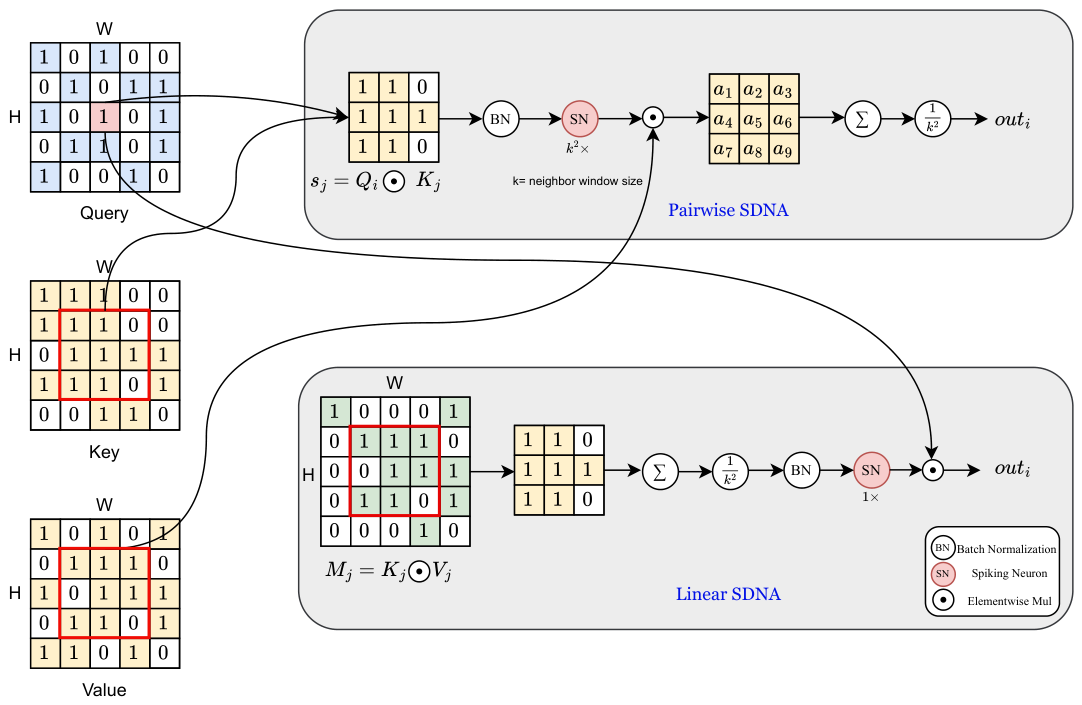
Figure 2.
Hierarchical architecture used for SDNA operators, each stage applies the SDNA operator at a fixed window with per-stage dilation.
Figure 2.
Hierarchical architecture used for SDNA operators, each stage applies the SDNA operator at a fixed window with per-stage dilation.
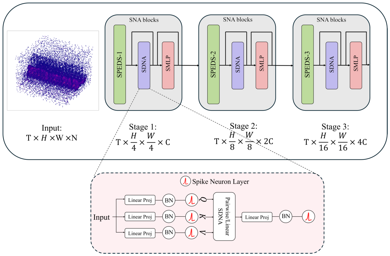
Figure 3.
Efficiency of the two operators as the neighborhood size k grows; all else fixed. (a) Inference throughput. (b) Peak memory.
Figure 3.
Efficiency of the two operators as the neighborhood size k grows; all else fixed. (a) Inference throughput. (b) Peak memory.
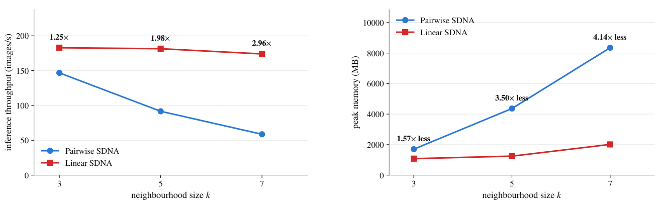
Figure 4.
Effect of gate calibration on N-Caltech101 (single seed, ablation configuration). (a) Gate firing rate, as a percentage of its maximum, across the three attention blocks, with and without the normalization. (b) Adding the channel-wise normalization on the gate input for both operators.
Figure 4.
Effect of gate calibration on N-Caltech101 (single seed, ablation configuration). (a) Gate firing rate, as a percentage of its maximum, across the three attention blocks, with and without the normalization. (b) Adding the channel-wise normalization on the gate input for both operators.
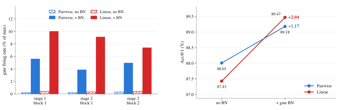

Table 1.
Per-group training and model settings for static image benchmarks (CIFAR-10, CIFAR-100), the large-scale ImageNet dataset and the neuromorphic benchmarks (N-Caltech101, DVS128-Gesture).
Table 1.
Per-group training and model settings for static image benchmarks (CIFAR-10, CIFAR-100), the large-scale ImageNet dataset and the neuromorphic benchmarks (N-Caltech101, DVS128-Gesture).
| Setting | CIFAR | ImageNet | Neuromorphic |
|---|---|---|---|
| Input | / | ||
| Patch size per stage | 1, 2, 4 | 4, 8, 16 | 8, 16 |
| Stages / blocks | 3 / 1, 1, 2 | 3 / 1, 2, 7 | 2 / 1, 1 |
| Embed dims | |||
| Dilation per stage | / | ||
| Epochs | 400 | 200 | 300 / 200 |
| Batch | 64 | 512 | 16 |
| Peak LR | |||
| Weight decay | |||
| MLP ratio | 4 | 4 | 1 |
Table 2.
Comparison of accuracy and parameter count on CIFAR10/100.
| Method | Architecture | Param | Time Step |
Accuracy | |
|---|---|---|---|---|---|
| CIFAR-10 | CIFAR-100 | ||||
| Spikformer [23] | Spikformer-4-384 | 9.32 | 4 | 95.51 | 78.21 |
| SDT [24] | S-Trans-2–512 | 10.28 | 4 | 95.60 | 80.02 |
| STAtten [39] | S-Trans-2–512 | 9.32 | 4 | 96.03 | 79.85 |
| QKFormer [31] | HST-4-384 | 6.74 | 4 | 96.18 | 81.15 |
| SWformer [40] | SWformer-4-384 | 7.51 | 4 | 96.10 | 79.30 |
| SAFormer [41] | SAFormer-4-384 | 9.32 | 4 | 95.80 | 79.07 |
| STMixer [42] | STMixer-4-384-32 | 8.29 | 4 | 96.01±0.11 | 81.87±0.16 |
| LSFormer [30] | LSFormer-4-384 | 9.50 | 4 | 96.73±0.07 | 82.00±0.04 |
| Pairwise SDNA | SDNA-4-384 | 6.76 | 4 | 97.24±0.08 | 81.73±0.22 |
| Linear SDNA | SDNA-4-384 | 6.79 | 4 | 96.87±0.09 | 80.98±0.13 |
Table 3.
Comparison of accuracy and parameter count on ImageNet.
| Method | Architecture | Param | Time Step | Accuracy |
|---|---|---|---|---|
| Spikformer [23] | Spikformer-8–384 | 16.81 | 4 | 70.24 |
| Spikformer-8–512 | 29.68 | 4 | 73.38 | |
| SDT [24] | S-Transfor-8-384 | 16.81 | 4 | 72.28 |
| S-Transfor-8-512 | 29.68 | 4 | 74.57 | |
| STAtten [39] | S-Transfor-8-512 | 29.68 | 4 | 76.18 |
| S-Transfor-8-768 | 66.34 | 4 | 78.11 | |
| Pairwise SDNA | SDNA-8-384 | 16.59 | 4 | 77.94 |
| SDNA-8-512 | 29.27 | 4 | 78.22 | |
| Linear SDNA | SDNA-8-384 | 16.59 | 4 | 77.67 |
| SDNA-8-512 | 29.27 | 4 | 77.93 |
Table 4.
Comparison of accuracy and parameter count on N-Caltech101 and DVS128-Gesture.
| Method | N-Caltech101 | DVS128-Gesture | ||||
|---|---|---|---|---|---|---|
| Param | Time Step | Accuracy | Param | Time Step | Accuracy | |
| Spikformer [23] | 2.57 | 16 | 83.6 | - | 16 | 98.30 |
| SDT [24] | 2.57 | 16 | 86.30 | - | 16 | 99.30 |
| LSFormer [30] | - | 10 | 87.60 ± 0.10 | - | 16 | 98.60 ± 0.30 |
| TIM [46] | - | 10 | 79.00 | - | - | - |
| QKFormer [31] | 1.57 | 16 | 87.24 | 1.5 | 16 | 98.60 |
| Pairwise SDNA | 1.95 | 16 | 88.95±1.08 | 1.92 | 16 | 98.89 ± 0.38 |
| Linear SDNA | 1.95 | 16 | 89.65±0.61 | 1.92 | 16 | 98.89 ± 0.29 |
Table 5.
Accuracy (%) under a homogeneous membrane time constant on the event benchmarks.
| N-Caltech101 | DVS128-Gesture | |||
|---|---|---|---|---|
| Pairwise | Linear | Pairwise | Linear | |
| 1.25 | 88.60 | 88.60 | 98.61 | 98.96 |
| 1.50 | 89.18 | 89.47 | 99.31 | 99.31 |
| 2.00 | 87.13 | 85.38 | 98.96 | 98.96 |
| 2.50 | 84.50 | 84.50 | 98.26 | 98.61 |
| 3.00 | 84.21 | 83.92 | 97.92 | 95.49 |
Disclaimer/Publisher’s Note: The statements, opinions and data contained in all publications are solely those of the individual author(s) and contributor(s) and not of MDPI and/or the editor(s). MDPI and/or the editor(s) disclaim responsibility for any injury to people or property resulting from any ideas, methods, instructions or products referred to in the content. |
© 2026 by the authors. Licensee MDPI, Basel, Switzerland. This article is an open access article distributed under the terms and conditions of the Creative Commons Attribution (CC BY) license.
Copyright: This open access article is published under a Creative Commons CC BY 4.0 license, which permit the free download, distribution, and reuse, provided that the author and preprint are cited in any reuse.