

Submitted:
31 August 2026
Posted:
31 August 2026
You are already at the latest version
Abstract
WiFi-based 3D reconstruction aims to recover articulated human pose, dense surface correspondence, parametric meshes, depth fields, point clouds, and spatial positions or trajectories from WiFi-derived measurements, including active Channel State Information (CSI) and passive WiFi radar observations. Recent methods increasingly draw on computer vision, yet it remains unclear which principles transfer effectively and which require WiFi-specific reformulation. Existing surveys address broader wireless sensing, CSI processing, deep learning, pose recognition, reproducibility, or generalisability, but do not jointly examine multiple 3D output representations and the strength of evidence behind vision-to-WiFi transfer. This survey reviews 34 methods through two independent dimensions: reconstruction target and output representation. The taxonomy covers full-body and multi-person reconstruction, hands and local body parts, moving objects, and indoor environments, represented as 3D skeletons, dense surface correspondence, parametric meshes, depth fields, point clouds, and spatial positions or trajectories. We explicitly distinguish commodity CSI, multi-link deployments, customised antenna geometries, and passive WiFi radar systems. We also audit dataset reuse, label provenance, evaluation practices, and diagnostic controls for testing signal dependence. Four evidence-qualified lessons concern structured output priors, observation consistency and identifiability, representation--architecture alignment, and acquisition- and domain-aware modelling. Together, these findings clarify current limitations and priorities for reproducible progress.
Keywords:
WiFi sensing
; 3D reconstruction
; wireless perception
; channel state information
; passive WiFi radar
; human pose estimation
; human mesh reconstruction
; point cloud reconstruction
1. Introduction
Three-dimensional reconstruction has undergone remarkable progress in computer vision, driven by advances in geometric representations, learning architectures, and large-scale annotated datasets. Modern vision systems can recover articulated human pose, dense surface correspondence, parametric body shape, and scene geometry with a level of accuracy and detail that has established vision-based 3D perception as a mature research area [1,2,3,4]. WiFi sensing, however, offers a fundamentally different yet compelling alternative. It enables contactless and device-free inference without a camera at deployment, although many current systems still rely on cameras, motion capture, depth sensors, or hand-tracking devices to generate training and evaluation references. Acquisition configurations also range from ordinary commodity links to multi-link deployments, customised antenna arrays, and synchronised passive WiFi radar receivers. WiFi sensing is particularly attractive under poor illumination, occlusion, or partial non-line-of-sight (NLoS) conditions. Nevertheless, it still raises important privacy and governance considerations, as it can infer human presence and activity without a visible sensing device. Despite recent progress, WiFi-based 3D reconstruction remains significantly less mature than its vision counterpart. This is largely because WiFi observations are indirect and sparse [5,6], strongly affected by multipath propagation [7], and often difficult to annotate at scale [8,9].
Recent advances demonstrate that WiFi sensing has progressed well beyond coarse tasks such as activity recognition, localisation, and presence detection toward richer forms of geometric understanding. Early studies, including Can WiFi Estimate Person Pose? [10] and WiPose [11], established the feasibility of recovering human body keypoints from commodity WiFi signals, with the former serving primarily as a 2D precursor and the latter demonstrating 3D skeleton reconstruction. Subsequent systems such as Winect [12], GoPose [13], and Person-in-WiFi 3D [14] extended this direction through free-form motion tracking, multi-link geometric reasoning, and Transformer-based 3D pose regression. More recent methods, including WiMTR [15] and MultiMesh [16], have further expanded the scope to multi-person pose and mesh reconstruction. Other recent studies have broadened the methodological focus to target-assisted domain adaptation, counterfactual regularisation, transceiver-geometry conditioning, topology-aware decoding, complex-valued sequence modelling, relative-pose and root-location decomposition, and self-supervised pretraining [17,18,19,20,21,22,23,24]. These mechanisms address different reconstruction, representation, and transfer problems and should not be interpreted as directly comparable solutions to one common form of domain shift.
Beyond articulated pose estimation, WiFi sensing has begun targeting denser geometric representations. DensePose From WiFi [25] demonstrated dense body-surface correspondence, while Wi-Mesh [26], MultiMesh [16], and WiMTR [15] explicitly pursued full-body mesh reconstruction using the Skinned Multi-Person Linear (SMPL) body model [27]. HandFi [28] and Wi-Hand [29] extend this progression to 3D hand-skeleton reconstruction and hand-mesh reconstruction using the MANO parametric hand model [30]. Emerging research is also exploring denser object- and scene-level outputs, including depth fields [31,32], object and indoor-scene point clouds [33,34], preliminary environmental point-cloud synthesis [35], and partial spatial outputs such as hand trajectories and 3D target positions [36,37].
Despite this progress, the literature remains fragmented. Existing methods target a wide range of outputs, from skeletons and meshes to depth fields and point clouds, and these output families have evolved at different rates. The central question is therefore no longer whether ideas from computer vision can be adopted, but which principles transfer conditionally, which require WiFi-native reformulation, and how strongly each WiFi-specific implication is supported by the available evidence. Answering this question requires separating modality-independent geometric structure from assumptions tied to image formation, while accounting for acquisition configuration, label provenance, domain variation, and evaluation protocol. To the best of our knowledge, existing surveys do not jointly address this gap. Existing surveys provide complementary views of the broader field. Liu et al. [6] review wireless techniques and applications for human activity sensing, while Xiao et al. [5] organise wireless device-free human sensing by task type and motion granularity. Wang et al. [7] focus on physical and model-based channel state information (CSI) sensing, and Nirmal et al. [38] and Ahmad et al. [9] examine deep-learning methods for radio-frequency (RF)- and WiFi-based human sensing. More recent surveys address public datasets, tools, code availability, and reproducibility [39], or generalisation across users, devices, and environments [40]. The most directly related prior review is the survey of skeleton-based human pose recognition using CSI by Wang et al. [41]. It covers CSI preprocessing, neural architectures, evaluation metrics, and several two- and three-dimensional skeleton-generation approaches. Its scope is nevertheless centred on skeleton and pose recognition and predates most subsequent work on multi-person metric 3D pose, dense surface correspondence, SMPL- and MANO-based meshes, depth fields, point clouds, self-supervised WiFi pretraining, and differentiable radio modelling. To the best of our knowledge, no prior survey jointly provides a target–representation taxonomy spanning these outputs, an acquisition-aware comparison, an audit of annotation provenance and output-specific evaluation, and an evidence-qualified analysis of lessons transferred from vision. Table 1 positions the present survey relative to these complementary reviews.
Scope and Contributions
This survey is a technical literature audit rather than a meta-analysis of recognition accuracy. Table 2 summarises the search strategy, inclusion criteria, and study-selection process. Our goal is to analyse WiFi-based 3D reconstruction as an output-centred problem rather than provide exhaustive coverage of all WiFi sensing research. We focus on methods whose inference-time input consists of WiFi-derived measurements and whose output is an explicit geometric representation, including 3D skeletons, dense surface correspondence, SMPL/MANO meshes, depth fields, point clouds, and spatial positions or trajectories. The methods covered in this survey span ordinary commodity CSI, commodity multi-link deployments, customised antenna geometries, and synchronised passive WiFi radar; these acquisition classes are reported separately and are not treated as directly comparable. Pure 2D pose estimation, activity recognition, identity recognition, received signal strength indicator (RSSI)-based localisation, and non-WiFi modalities are discussed only when they inform reconstruction, supervision, or evaluation. Throughout the survey, we distinguish between core, boundary, proxy, and related-only methods according to the nature of their geometric outputs.
Several related WiFi pose systems do not satisfy the core inclusion criterion but remain relevant to the development of input representations, learning architectures, and supervision strategies. These include CSIPose [42], HPE-Li [43], the adaptive-kernel multi-modal framework of Gian et al. [44], CSI-Former [45], MetaFi [46], MetaFi++ [47], PowerSkel [48], MpNet [49], the multiuser spatiotemporal method of Hsu and Hsieh [50], and MultiFormer [51]. They are treated as related-only when their principal reported output is two-dimensional, pose oriented without a clearly defined metric 3D output, or otherwise outside the geometric inclusion criteria of this survey.
The main contributions of this survey are as follows:
- Target–representation taxonomy and acquisition-aware comparison. We organise 34 methods along two independent dimensions: the reconstruction target and the output representation. The taxonomy separates full-body or multi-person, hand or local-part, moving-object, and indoor-environment targets from skeleton, dense-correspondence, parametric-mesh, depth-field, point-cloud, and spatial outputs. The methodological comparison reports sensing setup, WiFi observation, supervision source, and evaluation scope rather than imposing a global ranking across incompatible acquisition classes.
- Dataset, supervision, and evaluation audit. We distinguish reusable benchmarks from study-specific collections, document reference-label provenance, and distinguish routine agreement with camera- or software development kit (SDK)-derived labels from independent geometric validation, identifying where the latter is absent. We further organise evaluation by output representation and propose metric conventions together with diagnostic controls for testing signal dependence, temporal or deployment leakage, and annotation provenance.
- Evidence-qualified lessons from vision. After reviewing the WiFi literature and its evaluation evidence, we synthesise four lessons concerning structured output priors, observation consistency and identifiability, representation–architecture alignment, and acquisition- and domain-aware modelling. A consolidated assessment distinguishes broad adoption, controlled within-system results, strong corpus-wide absence findings, and WiFi-specific implications whose empirical validation remains immature.
- Recoverability- and benchmark-oriented research agenda. We identify future directions in recoverability-aware acquisition, calibrated observation-consistency mechanisms with ambiguity tests, representation–architecture co-design, hardware portability, variable-specific domain generalisation, data-efficient geometric learning, and output- and acquisition-specific benchmarks.
The remainder of the survey first introduces the WiFi sensing background and then reviews the surveyed literature through the target–representation taxonomy. It subsequently examines datasets and evaluation practices, synthesises lessons from vision after the WiFi evidence has been reviewed, discusses open challenges and future directions, and concludes the survey.
2. Background
WiFi sensing exploits the interaction of wireless signals with the surrounding environment through reflection, scattering, diffraction, absorption, and partial blockage by walls, furniture, and human bodies. As a result, the signal received by a WiFi device is a superposition of multiple delayed and attenuated copies of the transmitted waveform. This multipath propagation is fundamental to both the capabilities and challenges of WiFi sensing [6,7,39]. Figure 1 illustrates how line-of-sight, reflected, and body-scattered propagation paths contribute to the measured channel and how the resulting CSI observations can be organised across links, subcarriers, and packets.
2.1. Signal Propagation and Multipath
The received signal can be modelled as
where and denote the transmitted and received signals at frequency f and time t, respectively; is the channel frequency response, which captures both static environmental paths and dynamic paths induced by human motion; and represents additive noise [7,54]. Compared to optical sensing, WiFi operates at substantially longer wavelengths and provides much sparser observations. However, it offers several practical advantages, including infrastructure reuse, reduced direct capture of identifying appearance information, and robustness to poor illumination and partial occlusions [5,8,9]. At the same time, WiFi can infer human activities and motion without a camera and therefore should not be regarded as inherently privacy preserving.
2.2. CSI, Amplitude, and Phase
CSI describes the complex wireless channel response between a transmitter and receiver. In Orthogonal Frequency-Division Multiplexing (OFDM)-based WiFi systems, CSI characterises how the transmitted signal is attenuated and phase-shifted on each subcarrier for each transmit–receive antenna pair. Unlike RSSI, which provides only a coarse aggregate measure of received signal power, CSI provides fine-grained complex-valued measurements containing both amplitude and phase information. A single CSI coefficient can be written as where denotes the amplitude and denotes the phase. A full CSI capture from a commodity WiFi device is represented as a tensor where and are the numbers of transmit and receive antennas, is the number of OFDM subcarriers, and is the number of packets recorded over time. For visualisation, the transmit–receive antenna-pair dimensions can be indexed jointly as a link dimension L, giving the equivalent conceptual representation shown in Figure 1. On commodity hardware, the measured response additionally folds in transceiver-induced distortions such as carrier frequency offset and sampling time offset, so raw CSI phase typically requires calibration before use in downstream sensing tasks.
Early Intel 5300 CSI tools expose 30 subcarriers per stream, whereas more recent platforms such as Nexmon CSI, PicoScenes, and AX-CSI provide substantially higher subcarrier counts and bandwidths [39,54]. Spatial resolution is further constrained by antenna configuration. One-dimensional angle-of-arrival (AoA) estimation requires a linear array, whereas two-dimensional AoA estimation (azimuth and elevation) requires a planar or L-shaped array. Since commodity access points typically provide only one to three antennas arranged linearly, the spatially distributed multi-link configuration used by GoPose [13] and the customised L-shaped two-dimensional AoA apertures used by Wi-Mesh and MultiMesh [16,26] are not universally available. Consequently, the reported cross-environment results of these systems should be interpreted in the context of their hardware configurations. These link, subcarrier, and packet axes are measurement indices rather than direct Euclidean spatial coordinates. They nevertheless encode meaningful relationships across antennas or links, frequency, and time. Depending on bandwidth, antenna geometry, synchronisation, link configuration, calibration, and target motion, signal-processing methods can derive propagation-related quantities such as angle of arrival, angle of departure (AoD), time of flight (ToF), and Doppler from the measured channel [7,55]. The reviewed methods differ in whether they operate on raw or calibrated CSI, time–frequency representations, propagation-derived quantities, or learned tokens.
2.3. Common Preprocessing
Raw CSI measurements require preprocessing to mitigate noise, missing packets, phase offsets, and outliers [7,8,39]. Phase measurements are particularly challenging because the transmitter and receiver operate with independent oscillators. Consequently, carrier-frequency offset (CFO) and sampling-time offset (STO) introduce packet-dependent phase rotations that are unrelated to scene content. Antennas on the same receiver share a common clock, however, allowing calibrated phase differences to remain informative, although their reliability depends on antenna geometry, hardware calibration, and deployment conditions. Common preprocessing operations include interpolation, temporal smoothing, filtering, phase sanitisation, principal component analysis (PCA), and time–frequency transforms [8,9,54]. For example, DensePose From WiFi [25] employs phase unwrapping, filtering, and linear fitting, while WiMTR [15] unwraps CSI phase and removes a fitted linear slope and mean offset across subcarriers before Transformer tokenisation. These preprocessing choices determine which channel characteristics are preserved for downstream reconstruction. They do not, by themselves, establish which input representation or learning architecture is most effective. The next section organises the reviewed WiFi-based reconstruction methods jointly by reconstruction target and output representation. Their implications for transferring principles from vision are examined later in Section 5.
3. Taxonomy of WiFi-based 3D Reconstruction
Existing WiFi-based 3D reconstruction methods differ in both the reconstruction target and the geometric representation of the output. We therefore classify the surveyed literature along two independent dimensions. The target dimension distinguishes full human body or multiple people, hand or local body part, object or moving target, and indoor scene or environment. The representation dimension distinguishes 3D skeletons, dense surface correspondence, parametric meshes, depth fields, point clouds, and spatial positions or trajectories. Figure 2 cross-indexes the reviewed methods according to these dimensions.
This formulation separates what is reconstructed from how it is represented. Full-body reconstruction, for example, includes 3D skeletons, dense surface correspondence, and SMPL-based meshes, whereas point-cloud methods address either moving objects or indoor environments. DensePose From WiFi [25] is treated as a boundary case because it predicts body-region labels and UV coordinates rather than an explicit metric mesh. 3D-WiFi [37] and Passive Gesture [36] are treated as partial spatial outputs because they estimate, respectively, a 3D target location and a 3D hand trajectory without reconstructing a complete body, object, or scene.
3.1. 3D Skeleton Reconstruction
A 3D skeleton represents articulated pose as an ordered set of three-dimensional joint coordinates. It is the dominant output representation in the surveyed literature: 21 methods target full-body or multi-person reconstruction, while one method targets the hand.
Early systems established several recurring reconstruction strategies. WiPose [11], Wi-Mose [56], Winect [12], and GoPose [13] use temporal modelling, kinematic constraints, or propagation-derived motion and angular information to recover full-body joints. Compressed Representation [57] reduces the predicted pose space, whereas WiLink [58] selects informative links before skeletal regression. Person-in-WiFi 3D [14] extends skeleton prediction to multiple people. MDPose [59] reconstructs a 17-joint skeleton from passive-WiFi micro-Doppler observations, but its synchronised software-defined-radio configuration is materially different from ordinary commodity-CSI sensing.
More recent methods broaden the focus beyond basic in-domain skeletal regression. AdaPose [17], GenHPE [18], and PerceptAlign [19] address particular forms of configuration, environment, or layout variation. WiViPose [60], VST-Pose [61], Robust WiFi HPE [62], MultiDim-Fi [63], and WiFlow [64] introduce different temporal, denoising, feature-fusion, or supervision strategies. DT-Pose [20], GraphPose-Fi [21], C-MambaPose [22], RePos [23], and WiFi-JEPA [24] further investigate masked pretraining, topology-aware decoding, complex-valued sequence modelling, relative-to-absolute pose decomposition, or self-supervised representation learning. Because these systems differ in dataset, acquisition configuration, supervision, and evaluation protocol, their reported mechanisms and results are not directly comparable. HandFi [28] is the only surveyed skeleton method whose primary target is the hand. It predicts a palm-rooted skeleton together with an auxiliary binary hand mask from commercial WiFi measurements. Its skeletal topology connects five articulated finger-joint chains to a palm-centre root. The predicted mask is a two-dimensional auxiliary output rather than a reconstructed hand surface or depth field.
Multi-person reconstruction introduces an additional challenge that spans both skeleton and parametric-mesh outputs: the system must separate superposed reflections and associate each prediction with the correct subject. Person-in-WiFi 3D [14] uses query-based set prediction to recover multiple skeletons, while WiMTR [15] applies a query-based formulation to multi-person SMPL reconstruction. MultiMesh [16] instead detects and tracks subjects in propagation-derived profiles before applying a shared per-person SMPL regressor. These approaches solve related association problems but produce different outputs and use different acquisition pipelines. Current evidence also remains limited to small numbers of simultaneous subjects and largely fixed sensing configurations. Table 3 and Table 4 compare acquisition configuration, WiFi representation, supervision, and evaluation scope for skeleton and non-skeleton outputs, respectively.
3.2. Dense Surface Correspondence
DensePose From WiFi [25] is the only method in this category. For each detected person, it predicts DensePose correspondence: I assigns an image-domain body pixel to one of 24 predefined anatomical surface regions, while specifies a local coordinate within that region’s canonical two-dimensional chart. The method additionally predicts 17 two-dimensional keypoint heatmaps. These outputs map image-domain locations to a canonical body surface, but they do not instantiate a posed metric mesh or predict camera- or room-space coordinates, depth, body shape, global position, or mesh vertices. DensePose From WiFi is therefore treated as a dense-surface-correspondence boundary case rather than metric 3D reconstruction.
3.3. Parametric Mesh Reconstruction
Parametric-mesh methods recover an explicit articulated surface by regressing the parameters of a predefined body or hand model rather than predicting every vertex independently. Wi-Mesh [26], MultiMesh [16], and WiMTR [15] use SMPL to reconstruct full-body geometry, whereas Wi-Hand [29] uses the hand-specific MANO model. Wi-Mesh and MultiMesh derive propagation-organised angular profiles using customised antenna arrays before SMPL regression. WiMTR instead processes amplitude–phase CSI tokens from multiple receivers through a query-based Transformer, while Wi-Hand uses hand-specific angular representations before predicting MANO parameters. The category spans single-person body reconstruction, multi-person body reconstruction, and single-hand reconstruction. It also combines different antenna apertures, link configurations, input representations, and vision-derived supervision pipelines. All four methods demonstrate the feasibility of reconstructing fixed-topology parametric surfaces from WiFi, but none compares its body-model output with a capacity-matched unconstrained mesh decoder. Their adoption of SMPL or MANO should therefore be interpreted as a recurring representation choice rather than direct evidence that one parametric model or sensing pipeline is universally superior.
3.4. Depth-Field Reconstruction
Depth-field methods predict a dense depth value at each output location, providing a structured spatial field rather than articulated joints or a fixed-topology parametric surface. Wi-Depth [31] reconstructs foreground depth images of moving objects without modelling the static background. Its variational-autoencoder (VAE)-based teacher–student framework first learns a depth-image latent space and then maps CSI into that space, with auxiliary predictions for object shape, depth, and position. CSI2Depth [32] instead targets indoor human-centred scenes. It organises CSI amplitude and phase across antennas, subcarriers, and time, uses temporal and Transformer-based encoding, and applies a conditional generative model to synthesise depth images. Although both methods produce depth fields, they address different reconstruction targets and use different datasets, reference sensors, architectures, depth conventions, and evaluation protocols. Wi-Depth is evaluated on a study-specific moving-object collection, whereas CSI2Depth uses the WiFi and depth components of MM-Fi under cross-subject and cross-room evaluation. Their reported numerical results should therefore not be treated as direct cross-method comparisons.
3.5. Point-Cloud Reconstruction
Point-cloud methods represent geometry as unordered sets of three-dimensional points and therefore do not assume the fixed topology of SMPL or MANO. CSI2PC [33] targets controlled object-level reconstruction using a generative point-cloud architecture trained against paired object clouds. Määttä et al. [34] extend this direction to spatiotemporal indoor reconstruction on MM-Fi by converting amplitude and phase measurements into CSI tokens and using a Transformer encoder–decoder with learned point queries to predict fixed-size, LiDAR-derived point clouds. Pannone and Avola [35] instead first train a PointNet-based autoencoder on RGB/COLMAP scene clouds and subsequently learn a CSI encoder that maps paired ESP32 measurements into the resulting geometric latent space. These approaches differ substantially in target extent, acquisition hardware, point count, reference geometry, coordinate normalisation, registration, and evaluation metric. CSI2PC remains an object-level proof of concept, the MM-Fi method evaluates human-centred indoor geometry, and the Pannone–Avola system reports a preliminary room-level protocol. The category therefore demonstrates several possible CSI-to-point-cloud formulations, but it does not yet form a common benchmark or directly comparable reconstruction setting.
3.6. Spatial Position and Trajectory Estimation
This category contains explicit three-dimensional spatial outputs that do not reconstruct a complete articulated body, surface, object, or scene. 3D-WiFi [37] estimates a target position by combining azimuth, elevation, and an equivalent arrival-time measurement obtained with an external L-shaped antenna configuration. Its output is a single three-dimensional coordinate evaluated in controlled indoor localisation scenes. Passive Gesture [36] instead estimates a time-varying three-dimensional hand trajectory. It uses two WiFi links with linear antenna arrays to derive angular and path-length changes and is evaluated against Leap-Motion trajectories under user and environment variation. These methods are included as geometric proxies because their outputs have an explicit three-dimensional coordinate interpretation and help define the boundary between spatial sensing and complete reconstruction. Their tasks are nevertheless different: localisation estimates the position of a target, whereas trajectory reconstruction estimates a sequence of hand positions over time. Their numerical errors are therefore meaningful only within their respective coordinate frames, acquisition geometries, and trajectory or localisation protocols.
3.7. Cross-Method Comparison
The taxonomy contains 34 methods: 22 producing 3D skeletons, one dense surface-correspondence method, four parametric-mesh methods, two depth-field methods, three point-cloud methods, and two partial spatial-output methods. Of the 22 skeleton methods, 21 reconstruct the full body or multiple people and one reconstructs the hand. The literature therefore remains concentrated on full-body skeleton reconstruction, whereas hand, dense-surface, depth-field, and point-cloud reconstruction are represented by much smaller groups. Cross-method comparison requires agreement in reconstruction target, output representation, sensing configuration, dataset, split, coordinate convention, alignment procedure, and evaluation metric. Joint-position errors are not directly comparable with mesh-vertex, depth, point-cloud, localisation, or trajectory errors. Table 3 and Table 4 therefore report sensing setup, WiFi observation, reference labels or supervision, and evaluation scope without imposing a global performance ranking.
Sensing Configuration and Recoverability
The output representation alone does not determine the difficulty of a reconstruction problem. Recoverability also depends on signal bandwidth, antenna aperture and geometry, the number and placement of transmitter–receiver links, temporal observation length, hardware synchronisation, and calibration. Systems using customised arrays, multiple spatially separated links, or synchronised passive-radar receivers may estimate angle, delay, or Doppler with dimensionality or resolution that is unavailable in a typical few-link commodity-CSI deployment. These acquisition conditions must be reported alongside reconstruction results and considered before comparing architectures or numerical accuracy.
4. Datasets, Evaluation, and Benchmarks
The evaluation ecosystem for WiFi-based 3D reconstruction remains fragmented across study-specific collections, sensing configurations, label-generation pipelines, and output-dependent metrics. A numerical result is therefore meaningful only together with its acquisition setup, reference-label provenance, split, coordinate convention, alignment procedure, and metric definition. This section separates three questions that are often conflated: which datasets are reused, what their reference labels represent, and how each geometric output is evaluated. It then proposes output-specific reporting protocols and diagnostic controls. Recording duration, CSI-packet counts, labelled frames or windows, and sequence counts are treated as distinct quantities rather than combined in one scale column, because the source papers report them in incompatible units.
4.1. Dataset Landscape and Reuse
Table 5 summarises the principal reusable datasets and category-defining study-specific collections. It distinguishes reusable resources from study-specific collections and reports acquisition, reference-label provenance, and domain shift, including MDPose’s distinct passive WiFi radar protocol [59]. Early 3D-skeleton systems were evaluated mainly on study-specific collections tied to particular rooms and deployments. WiPose [11], Winect [12], and GoPose [13] established feasibility under distributed-receiver, free-form, and multi-link angle-of-arrival configurations, respectively, but none defines a shared benchmark split that is broadly reused by later work. PiW3D [14] contains single- and multi-person 3D pose annotations from three indoor environments and is reused by DT-Pose [20], GenHPE [18], RePos [23], and WiFi-JEPA [24]. MM-Fi [52] contains 40 subjects and four environments with synchronised WiFi and complementary modalities and defines S1, S2, and S3 random, cross-subject, and cross-environment protocols. Because its WiFi observations use one hardware configuration, S3 tests environmental transfer rather than cross-device or cross-chipset generalisation.
Recent collections target limitations not represented by these benchmarks. PerceptAlign [19] introduces three primary scenes with 21 participants, including three transceiver layouts in the office scene, together with two additional held-out test scenes; seven layouts are represented overall. The collection supports in-domain, leave-one-scene-out, and within-scene cross-layout evaluation. DensePose From WiFi [25] reuses a collection containing eight subjects, one–five simultaneous people, and 16 spatial layouts: six recordings in a laboratory office and ten in a classroom. Its in-deployment protocol randomly divides samples from all 16 layouts into 80% training and 20% testing, while its layout-shift experiment trains on 15 layouts and tests on one fixed unseen classroom layout. Wi-Depth [31] collects paired CSI and depth observations from six volunteers in four environments and applies leave-one-subject-out evaluation separately within each environment. Point-cloud and depth methods otherwise either reuse MM-Fi, as in CSI2Depth [32] and Määttä et al. [34] or rely on task-specific collections, as in CSI2PC [33] and Pannone and Avola [35]. Consequently, no shared benchmark currently spans skeletons, dense correspondence, meshes, depth fields, point clouds, and trajectories under a common acquisition protocol.
4.2. Reference Labels, Provenance, and External Validation
WiFi-based reconstruction requires geometric references for supervision and evaluation, but these references are produced in different ways. The surveyed literature uses motion capture, RGB-D or hand-tracking SDKs, direct depth or range measurements, vision-generated pseudo-labels, and annotations inherited from public benchmarks. These sources differ in accuracy, coordinate convention, calibration requirements, visibility limitations, and failure modes. Consequently, a reported reconstruction error should be interpreted together with both the provenance of the reference geometry and the role that it plays in the experimental pipeline.
Three roles should be distinguished. First, a reference may provide training supervision. Second, the same source may define the routine evaluation target against which prediction error is reported. Third, an additional source that is not used for training or routine model selection may provide external geometric validation. The first two roles measure agreement with an operational annotation source; they do not independently establish absolute geometric accuracy. This distinction applies even when the reference sensor is physically separate from the WiFi system. For example, Mocap in WiPose [11] and MDPose [59], Kinect or Azure Kinect in Winect and Person-in-WiFi 3D [12,14], and Leap Motion in HandFi [28] provide geometrically meaningful targets, but they primarily serve as supervision or routine evaluation references within the corresponding studies. Other methods depend on labels produced by vision pipelines rather than direct geometric sensors. DensePose From WiFi [25] uses DensePose [1] and keypoint pseudo-labels together with an RGB feature teacher; Wi-Mesh [26], WiMTR [15], and Wi-Hand [29] use camera-derived parametric-body or hand-model labels; AdaPose [17] uses HRNet-derived pose supervision in its study-specific setting; and PerceptAlign [19] uses EasyMocap-derived joints. Performance measured against these labels primarily quantifies agreement with the corresponding vision-based annotation pipeline. Without a third reference, disagreement between the WiFi estimate and the vision teacher does not reveal which estimate is geometrically more accurate. Figure 3 summarises these roles. It distinguishes the annotation source used for supervision and routine evaluation from an additional external reference that can independently audit both the operational labels and the WiFi prediction.
Several reviewed systems further show why annotation provenance must be reported at the level of the complete pipeline. MDPose [59] uses Mocap trajectories to provide joint positions, derived velocities, pose-correction targets, and inputs to its micro-Doppler simulator. HandFi [28] obtains joint coordinates from Leap Motion but generates its auxiliary hand masks using GrabCut. DensePose From WiFi [25] separates the generation of DensePose and keypoint pseudo-labels from the RGB feature-teacher pathway. WiMTR [15] and Wi-Hand [29] evaluate reconstructed meshes against camera-fitted SMPL [27] or MANO [30] references rather than against independently measured surface geometry.
4.3. Evaluation Practices and Output-Specific Protocols
Evaluation practices vary across output representations. Skeleton studies commonly report mean per-joint position error (MPJPE), Procrustes-aligned MPJPE (PA-MPJPE), and percentage of correct keypoints (PCK). Mesh studies use per-vertex error (PVE) or mean per-vertex position error (MPVPE), while dense-correspondence methods use geodesic point similarity (GPS) and its masked variant (GPSm). These metric names alone do not establish comparability. Absolute, root-centred, and Procrustes-aligned joint errors answer different questions; registered point-cloud error is not equivalent to unaligned error; and DensePose GPS measures canonical-surface correspondence rather than metric 3D geometry.
Table 6 combines metrics observed in the literature with reporting conventions and diagnostic controls suggested by this survey. Several reviewed papers illustrate the remaining ambiguity. WiMTR’s vertex alignment terminology is inconsistent [15]; Wi-Hand [29] and HandFi [28] do not define root or Procrustes alignment; MDPose [59] reports mean absolute keypoint error rather than an alignment-defined MPJPE; and DensePose From WiFi [25] reports canonical geodesic similarity, with one inconsistent GPSm value across source tables. Such details should be recorded, but they do not require separate main-text audits for every method. A benchmark should establish that performance depends on the measured CSI rather than only on output priors, temporal regularity, or deployment leakage.
4.4. Benchmark Controls and Reporting Considerations
The reviewed evaluations rarely test whether reconstruction depends on the corresponding WiFi observation rather than on output regularity, temporal predictability, or deployment-specific correlations. We therefore suggest several diagnostic controls, applied where relevant: output-prior or nearest-neighbour baselines; constant-input or no-CSI evaluation; CSI shuffling; temporal-only prediction for sequential outputs; and room-, layout-, or link-metadata-only baselines. An additional geometric reference, when available, can also help distinguish reconstruction error from disagreement with the operational annotation pipeline.
Representation comparisons are most informative when alternatives are evaluated within the same implementation, dataset, and protocol. Accompanying differences in preprocessing, calibration, temporal context, input dimensionality, model capacity, and computation should be reported, because improvements cannot be attributed to representation alone when several pipeline components change simultaneously. Prior WiFi and RF sensing surveys identify incomplete hardware descriptions, inconsistent protocols, and unavailable data or code as major barriers to reproducibility [38,39,40]. Reconstruction studies should therefore report the sensing hardware and layout, bandwidth and subcarriers, synchronisation and calibration, input representation, supervision source, dataset split, coordinate and alignment conventions, metrics, and data/code availability. Recording duration, CSI packets, labelled samples, and sequences should be reported separately. Future benchmarks would also benefit from output-specific tracks that distinguish commodity few-link CSI, multi-link deployments, customised arrays, and passive or synchronised WiFi radar.
5. Lessons from Vision for WiFi-Based 3D Reconstruction
This section uses vision-based 3D reconstruction not as a source of methods to be transferred directly, but as an analytical reference against which WiFi-based reconstruction can be understood. Decades of research in computer vision have established the structural reasons for the success of vision-based 3D reconstruction, namely the properties of cameras and image observations that make modern reconstruction pipelines effective. Comparing WiFi sensing against this reference helps distinguish components that are largely modality-independent from those that depend fundamentally on camera-specific observation physics. The former can often be transferred with minimal modification, whereas the latter require substantial reformulation.
The preceding taxonomy and evaluation audit establish substantial variation across reconstruction targets, output representations, sensing configurations, supervision sources, and experimental protocols. This section synthesises that evidence through four questions: how geometric output structure is incorporated into WiFi reconstruction; whether predicted geometry can be related back to the measured wireless observation and under what conditions it is identifiable; how input representation should be matched to network architecture; and how acquisition and domain variation are handled. The final subsection distinguishes findings supported across multiple methods from system-specific evidence and open research hypotheses.
5.1. Structured Output Priors
Modern vision systems employ a wide range of geometric representations, including keypoints [65], dense correspondence [1], parametric meshes [2,3,27], point clouds [66], depth fields [67], and implicit surfaces [4,68,69]. A particularly important lesson for WiFi sensing is the value of parametric body models such as SMPL [27], which reduce a human body from 20,670 vertex coordinates to 82 parameters. Such low-dimensional representations were transformative for vision and are arguably even more important for WiFi, where sparse observations require stronger constraints on the output space.
An output prior specifies structural properties that the reconstructed geometry is expected to satisfy. Parametric models such as SMPL [27] and MANO [30] encode fixed mesh topology, articulated joint structure, and learned variation in body or hand pose and shape. Skeleton graphs and kinematic constraints serve a related purpose by defining joint connectivity, bone relationships, or anatomically valid configurations. Consequently, they transfer naturally across sensing domains. This pattern is evident throughout the surveyed literature: mesh-reconstruction systems consistently employ SMPL or MANO, while articulated-pose methods rely on skeletal constraints of some form.
DensePose From WiFi [25] provides a related but non-metric example of structured surface prediction. Its output is constrained by the predefined DensePose atlas: a fixed canonical body surface divided into 24 anatomical regions, with a separate local chart for each region. This representation imposes anatomical organisation and canonical geodesic relationships without decoding a posed body mesh. The paper demonstrates WiFi-to-canonical-surface correspondence, but it does not compare the DensePose atlas against an unstructured dense-pixel output, a direct metric surface, or an alternative correspondence representation. It therefore contributes adoption evidence for a structured surface prior, not a controlled output-prior ablation.
For Wi-Mesh [26], the prior is explicit: the network predicts 72 SMPL pose values and ten shape coefficients, which are decoded into a fixed-topology 6,890-vertex mesh. This demonstrates adoption of a compact structured surface representation and the feasibility of WiFi-to-SMPL prediction. Its reported baselines, however, replace the two-dimensional AoA input with raw CSI, Doppler, or separate one-dimensional AoA spectra while retaining the same stated Wi-Mesh learning model. They therefore compare input representations rather than the SMPL prior. Wi-Mesh provides no SMPL-versus-direct-vertex or other matched output-prior ablation. MultiMesh extends this adoption pattern to two- and three-person scenes. For each signal-space detection and track, it predicts 72 SMPL pose values and an unspecified-dimensional shape vector, which gender-neutral SMPL decodes into a 6,890-vertex mesh [16]. This shows that the parametric prior remains the chosen output representation when the problem is expanded from one person to several simultaneously observed people. It does not provide a controlled body-model comparison: the reported baselines vary the propagation dimensions used for subject separation and per-person input construction while retaining the SMPL surface model. WiMTR [15] extends the same adoption pattern to joint multi-person set prediction. It predicts 24 joint rotations in a six-dimensional representation and ten SMPL shape coefficients for each selected person, which are decoded into a fixed-topology 6,890-vertex body mesh. Its ablations vary phase input, phase sanitisation, the refine decoder, and joint-query generation while retaining SMPL throughout. It therefore provides no SMPL-versus-direct-vertex or other matched output-prior comparison.
Wi-Hand [29] extends the parametric-prior adoption pattern from the full body to the hand domain. It predicts 48 MANO pose values and ten shape coefficients, which are decoded into a fixed-topology 778-vertex hand mesh. Its signal-representation and network ablations all retain MANO, and the method defines no separate anatomical, bone-length, joint-limit, collision, or kinematic loss whose effect is independently tested. Its structural restriction is supplied primarily by the MANO model itself. Wi-Hand therefore provides direct evidence of MANO-prior adoption and WiFi-to-MANO feasibility, but no controlled comparison against an unconstrained hand-mesh output.
Thus, Wi-Mesh, MultiMesh, WiMTR, and Wi-Hand provide direct evidence of parametric-prior adoption and WiFi-to-SMPL/MANO feasibility, but their experiments do not quantify the gain from these models against matched unconstrained surface decoders. The direct output-structure ablation evidence currently comes primarily from skeletal decoders and anatomical losses rather than from the parametric-mesh systems. GraphPose-Fi [21] reports 167.8 mm MPJPE with a multilayer perceptron (MLP) regression head and 160.6 mm with its complete graph-based regression head in its MM-Fi ablation setting; the encoder and LTSA module are held fixed, but the comparison does not isolate skeletal topology from self-attention and other architectural differences within the regression head. On MM-Fi P1–S1, DT-Pose [20] reports 197.4 mm MPJPE for its MLP-only decoder and 165.3 mm for the complete task-prompt, graph convolutional network (GCN), and Transformer decoder. This endpoint comparison supports the complete joint-oriented decoder, but it conflates task prompting, graph processing, Transformer processing, decoding depth, and other architectural differences. In a more closely matched comparison, adding the GCN to the task-prompt–Transformer configuration changes MPJPE from 167.1 to 165.3 mm, providing smaller component-level evidence for the graph-processing stage. On MM-Fi P1–S3, replacing the complete GraFormer decoder in C-MambaPose [22] with the evaluated MLP decoder increases MPJPE from 298.5 to 358.9 mm, while setting the bone-length-loss coefficient to zero increases MPJPE to 314.3 mm. The corresponding PA-MPJPE values are 102.2, 103.2, and 102.4 mm for the complete, MLP-decoder, and no-bone-loss variants, respectively. These ablations provide method-specific evidence for the complete topology-aware decoder and supervised bone-length-consistency loss, but they do not isolate skeletal topology alone.
HandFi [28] provides a comparatively direct anatomical-loss comparison for hand reconstruction. Its palm-rooted model defines five palm–CMC–MCP–PIP–DIP chains and applies a joint-coordinate term, valid ranges for 15 articulated finger-bone lengths, and angle and curvature constraints over the five palm-to-CMC bones. Relative to the preceding multi-task configuration with the same complex-signal embedding, shared encoder, mask branch, and focal-style mask loss, adding the complete pose-constraint package reduces MPJPE from 5.72 to 2.07 cm and increases PCK@2 cm from 0.76 to 0.93. The results are reported as averages over five runs. This is direct within-system evidence for the complete anatomical-loss package. It does not isolate the bone-length term, palmar-angle term, or palmar-curvature term individually, and the source is not fully explicit about whether its DeepCORAL term is active in this particular main-dataset ablation. The result should therefore not be attributed to one anatomical constraint in isolation.
The supported lesson is therefore qualified. Structured output priors are among the clearest transfers from vision because they constrain the geometry without requiring WiFi observations to share image-plane organisation. Their adoption does not, however, establish how strongly a prediction depends on the measured WiFi input. A model can potentially produce plausible geometry from output statistics, temporal regularity, or deployment correlations. Prior-constrained systems should therefore be evaluated with the output-prior, constant-input, CSI-shuffling, nearest-neighbour, and temporal-only controls defined in Section 4.4.
5.2. Observation Consistency and Identifiability
Perhaps the most significant development in vision-based reconstruction has been the shift from direct regression to reconstruction-aware learning, in which models are required to explain the input observations through a differentiable forward model. In HMR [2], a convolutional neural network (CNN) predicts SMPL pose and shape parameters from a single image. The resulting mesh is projected through a camera model, and its predicted two-dimensional joints are compared with image keypoint annotations. Related differentiable-rendering methods additionally compare predicted silhouettes or rendered appearance with image evidence. The transferable principle is that predicted geometry can be checked against information in the observation or annotation domain. NeRF [4] extends the same principle to scene reconstruction. A neural network represents the scene as a continuous radiance field, and novel views are generated through differentiable volume rendering by integrating colour and density along camera rays. Training requires only posed images because the rendering process itself provides the supervisory signal.
These examples should not be treated as identical forms of supervision. HMR enforces consistency with image-derived keypoint annotations, whereas photometric methods such as Monodepth2 [67] and rendering-based methods such as NeRF compare synthesised and observed image evidence. The transferable principle is that a predicted geometry can be checked against information in the observation or annotation domain.
Across the 34 WiFi reconstruction methods reviewed in this survey, learned estimators use externally defined geometric targets for task supervision, while analytical or model-based systems are evaluated against external geometric references. These include motion-capture joints, RGB-D or sensor-SDK estimates, vision-generated pseudo-labels, inherited benchmark annotations, depth images, point clouds, and spatial coordinates, as documented in Table 3 and Table 4 and in Section 4.2. Within the surveyed corpus, we did not identify a method that maps its own predicted geometry into an expected wireless observation and compares that prediction with the corresponding measured observation as a task-level reconstruction loss. DensePose From WiFi’s image-teacher transfer is not an exception [25]. It compares intermediate feature pyramid network (FPN) features from the WiFi student with features extracted from synchronised RGB images and supervises the final correspondence using vision-generated pseudo-labels. The predicted correspondence is never used to generate an expected CSI measurement, and no predicted wireless observation is compared with the measured CSI. Self-supervised CSI representation learning does not change this finding. DT-Pose [20] combines masked WiFi reconstruction, temporal-consistent contrastive learning, and uniformity regularisation during input-side self-supervised pretraining; the pretrained encoder is then frozen for supervised pose decoding. WiFi-JEPA [24] predicts masked target-encoder CSI embeddings from visible time–link tokens during self-supervised pretraining and subsequently fine-tunes the encoder and pose estimator end-to-end using labelled 3D skeletons. MDPose [59] uses recorded Mocap trajectories to drive SimHumalator and produce matched synthetic micro-Doppler spectrograms. These simulations define the clean domain used by the measured-spectrogram denoiser and train the velocity estimator that is subsequently applied to denoised measurements. GenHPE [18] instead trains an RF generator on source-domain ground-truth skeletons and uses full-skeleton and body-part-removed generations as privileged regularisation during training. In both cases, the forward direction is conditioned on reference skeletons rather than on the reconstruction model’s own output. Neither method passes its final predicted skeleton through the simulator or generator, and neither compares a prediction-conditioned wireless observation with the corresponding measured input. A generic observation-consistency formulation can be written as:
where denotes the predicted geometry, describes the propagation environment, describes the transmitter and receiver configuration, and represents hardware and calibration parameters. The predicted observation may be CSI, a channel response, or another measurement appropriate to the acquisition system. A corresponding consistency term is:
Equations (2) and (3) are a proposed abstraction, not a capability demonstrated by the reconstruction methods reviewed in this survey. Differentiable radio research provides partial components: Sionna RT [70] computes differentiable channel responses for specified scenes and radio configurations; DiffeRT [71] supports gradient-based radio propagation optimisation; Learning Radio Environments [72] estimates material and scattering parameters from measured channel data; and RayLoc [73] formulates localisation as an inverse differentiable-ray-tracing problem using commodity WiFi CSI. These studies do not demonstrate a calibrated training-loop model that accepts an unknown dynamic body or scene geometry, predicts the associated WiFi measurement, and propagates the resulting gradient to a skeleton, mesh, depth-field, or point-cloud estimator.
Observation consistency must also be separated from identifiability. A low would show that a candidate geometry is compatible with an adopted forward model and acquisition configuration. It would not show that this geometry is the unique physical configuration capable of producing the observation. Limited bandwidth, antenna aperture, link diversity, calibration accuracy, and temporal context may allow different combinations of geometry, position, body shape, environmental paths, or hardware parameters to produce similar modelled measurements. The surveyed studies do not test this possibility by searching for distinct geometries that explain the same observation. Cross-environment degradation should likewise not be attributed specifically to the absence of an observation-consistency loss. Current protocols simultaneously vary multipath, transceiver placement, link diversity, subject distribution, calibration, label provenance, and coordinate conventions. The available experiments do not isolate a missing forward loop from these other sources of variation.
The transferable lesson is therefore not to copy a camera-projection or rendering equation, but to constrain reconstruction, where feasible, using evidence related to the observation from which it was inferred. Any WiFi forward model or learned surrogate must be evaluated for calibration, geometric sensitivity, approximation error, and ambiguity under the intended acquisition configuration. This lesson therefore contains two findings with different evidential status. First, the corpus-level finding is that we did not identify a surveyed WiFi reconstruction method that passes its own final predicted geometry through a forward wireless model and compares the resulting observation with the corresponding measurement as a task-level loss. Second, the vision-derived transfer proposal remains empirically immature: it is not yet known whether adding such a constraint improves reconstruction, transfer, or dependence on sample-specific CSI. The low validation level in Figure 4 refers only to this second point; it does not imply that observation consistency is an unimportant or weak lesson.
5.3. Representation–Architecture Alignment
A raw CSI tensor is organised along three principal dimensions: transmitter–receiver antenna pairs, OFDM subcarriers, and time samples. Each entry in this tensor represents a superposition of contributions from all active propagation paths present at the time of measurement. The subcarrier dimension specifies the frequency bin within the channel bandwidth at which the channel response is sampled, while the antenna dimension identifies the transmitter–receiver pair associated with the measurement, reflecting the underlying array configuration rather than any location within the physical scene. Crucially, neither dimension corresponds directly to spatial position. CSI nevertheless has a meaningful internal organisation. Subcarriers sample the channel at different frequencies, consecutive packets capture temporal variation, and antenna pairs or spatially separated links provide distinct views of the propagation field. These relationships support frequency-domain processing, temporal modelling, and cross-link aggregation, although their organisation differs fundamentally from the Euclidean locality of neighbouring image pixels. Propagation-derived representations such as angle of arrival, angle of departure, time of flight, and Doppler can further expose directional, delay, and motion-related structure. Their availability and resolution depend on bandwidth, antenna aperture and geometry, synchronisation, calibration, link placement, and temporal context [7,55,59].
Convolution and attention can therefore remain appropriate for WiFi sensing when the input representation exposes relationships that these operations can exploit. The key design question is not whether a particular learning operation is suitable in isolation, but whether its inductive bias matches the organisation of the represented measurements. This distinction motivates treating representation and architecture as separate but coupled design decisions. The representation determines which relationships are preserved, derived, or made explicit, while the architecture determines how those relationships are processed. Reported improvements may also reflect calibration, denoising, temporal context, input dimensionality, model capacity, optimisation, or hardware configuration. Architectural and representation claims should therefore be interpreted together with the complete experimental pipeline.
The reviewed methods illustrate several alignments. DensePose From WiFi [25] translates separate amplitude and sanitised-phase CSI features through MLP and convolutional processing into an image-like representation, enabling reuse of a modified DensePose-RCNN with FPN, region proposals, region-of-interest (ROI) processing, dense correspondence, and keypoint heads. This is an explicit modality-translation design: the CSI axes themselves are not treated as image-plane coordinates; a learned stage constructs the image-like representation before the vision architecture is applied. Wi-Mesh [26] applies ResNet-18 [74] processing to azimuth–elevation spectra derived through four-dimensional MUSIC [75], then uses a two-layer gated recurrent unit (GRU) [76] and temporal self-attention to aggregate 15 frames from two receiver viewpoints. MultiMesh [16] couples four-dimensional propagation estimation with signal-space subject detection and tracking, then applies a ResNet, a two-layer GRU, and temporal self-attention to the resulting person-specific azimuth–elevation sequences. WiMTR [15] flattens receiver, antenna, and time coordinates into 180 tokens containing amplitude and linearly sanitised phase features across 30 subcarriers, applies modality-specific MLP projections and a six-layer Transformer encoder [77], and uses human, identity, and joint queries for coarse-to-fine multi-person mesh regression. HandFi [28] normalises the measured complex CSI by packet power, represents each of the three receive streams through paired real and imaginary channels over 114 subcarriers and 20 packets, and uses bias-free grouped convolutions to embed the complex components without mixing different antenna streams prematurely. A shared multi-scale encoder then feeds separate decoders for the palm-rooted 3D skeleton and dense two-dimensional hand mask. This aligns complex signal organisation with antenna-specific embedding and uses the mask as an auxiliary dense task rather than as an explicit geometric input to the pose decoder. MDPose [59] uses CLEAN-processed and FMNet-denoised time–micro-Doppler spectrograms, applies convolutional feature extraction and a two-layer bidirectional long short-term memory (LSTM) network to estimate three-dimensional velocities for 17 keypoints, recursively integrates those velocities into joint positions, and uses a separate bidirectional-LSTM optimisation network to initialise and periodically correct the pose trajectory; GraphPose-Fi [21] processes a preprocessed real-valued antenna-pair–subcarrier–time tensor derived from raw complex CSI before using a graph-based skeletal head; WiFi-JEPA [24] retains a factored channel–time–link representation during masked latent pretraining, with each token corresponding to one time–link coordinate and containing amplitude and denoised-phase subcarrier features; and C-MambaPose [22] uses a complex-valued phase branch and a real-valued amplitude branch, fuses their features in complex space, processes the fused sequence with Complex Mamba, and projects the result to magnitudes before joint-query mapping and GraFormer decoding.
DensePose From WiFi [25] reports a staged same-layout ablation. Amplitude-only input gives DensePose average precision (dpAP) combined with GPS and GPSm, denoted dpAP·GPS and dpAP·GPSm, respectively, of 40.6 and 39.7; adding sanitised phase gives 41.2 and 40.1; adding auxiliary keypoint supervision gives 44.6 and 42.9; and adding image-teacher FPN transfer gives 45.3 and 43.2. This provides modest within-system evidence for phase inclusion and stronger endpoint evidence for the combined keypoint-supervision and teacher-transfer pathway. The sequence is cumulative, however, and does not isolate all components independently. In particular, the 40.1-to-42.9 and 42.9-to-43.2 changes reflect changes in supervision rather than only changes in input representation or network architecture. The paper also does not compare its learned CSI-to-image translation with a capacity-matched CSI-native detector, alternative tokenisation, or direct non-image correspondence decoder. The ablation therefore supports the evaluated complete pipeline, not a universal advantage for image-like translation or DensePose-RCNN.
Wi-Mesh [26] also provides a within-system comparison of input representations. Using data from the same collection and the same stated deep-learning model, its raw-CSI baseline reports 12.14 cm PVE and 9.75 cm MPJPE, the Doppler baseline reports 6.01 and 4.51 cm, and the separate one-dimensional-AoA baseline reports 4.10 and 3.51 cm. The complete azimuth–elevation representation reports 2.81 cm PVE and 2.40 cm MPJPE. This supports the adopted two-dimensional AoA representation within the customised dual-receiver array and processing pipeline. It does not establish that the same representation is available or superior under few-antenna commodity deployments, and the comparison does not isolate representation from its associated calibration, four-dimensional MUSIC processing, tensor organisation, or computational cost. The paper also does not state whether its PVE and MPJPE are root-aligned, rigidly aligned, scale-aligned, or Procrustes-aligned.
MultiMesh [16] provides a related within-system comparison of propagation dimensions while retaining its deep mesh-construction framework. For two-person scenes, using azimuth and ToF gives PVE, root-matched MPJPE, and PA-MPJPE values of 9.93, 8.91, and 4.45 cm; adding AoD gives 6.29, 5.62, and 2.76 cm; using azimuth, elevation, and ToF gives 4.93, 4.05, and 2.37 cm; and the complete azimuth–elevation–AoD–ToF pipeline gives 4.01, 3.51, and 1.90 cm. For three-person scenes, the corresponding values are 11.26/10.25/5.15, 8.01/7.23/3.56, 6.54/5.18/2.81, and 5.39/4.65/2.43 cm. These experiments support the richer multidimensional propagation and subject-separation pipeline within the customised 3-Tx-by-9-Rx configuration. They do not isolate the value of one neural architecture or of SMPL: changing the available propagation dimensions also changes source resolvability, person detection, reflection filtering, and the construction of each person-specific input. The comparison therefore supports the complete representation-and-separation pipeline rather than a universal ranking of azimuth, elevation, AoD, or ToF.
WiMTR [15] provides smaller component-level comparisons under a common 30-epoch ablation setting. With the refine decoder and differentiated joint queries fixed, amplitude-only input gives 78.5 mm MPJPE, 32.3 mm PA-MPJPE, and 96.3 mm PVE; raw phase gives 77.9, 31.9, and 95.3 mm; and linearly sanitised phase gives 76.9, 31.0, and 94.3 mm. These results provide modest within-system evidence for including phase and for the evaluated sanitisation relative to raw phase. Removing the refine decoder gives 78.6/32.4/96.0 mm, while replacing identity-conditioned differentiated joint queries gives 77.4/31.5/94.8 mm. The latter differences are only 0.5 mm on each reported metric. All of these variants are trained for 30 epochs, whereas the principal 71.4/29.7/57.3 mm model is trained for 100 epochs; the main and ablation scores should therefore not be mixed. The ablations support the evaluated phase-processing, refinement, and query-generation components, but do not establish that Transformer tokenisation is superior to a matched CNN, recurrent, image-like, or factorised-token alternative. Repeated-run variance and significance tests are not reported.
Wi-Hand [29] reports a larger within-system comparison of propagation-derived inputs while retaining its MANO reconstruction network. Raw CSI gives 7.28 cm MPVPE, 6.45 cm MPJPE, and 0.24 PCK@1.5 cm; Azimuth–ToF gives 5.32, 4.41, and 0.39; adding elevation gives 2.24, 1.95, and 0.60; adding AoD gives 1.47, 1.36, and 0.71; and the complete pipeline, which also uses Doppler to suppress body and arm reflections, reports 1.05, 0.99, and 0.85. A random-mesh sanity baseline gives 9.56 cm MPVPE, 8.84 cm MPJPE, and 0.12 PCK. These comparisons support the complete multidimensional signal-separation and hand-specific AoA representation within the customised 3-Tx-by-9-Rx system. They do not isolate individual propagation variables cleanly: adding a dimension changes target separation, clutter filtering, and the input supplied to the network. They also do not test MANO, since every learned variant retains the same parametric hand model. The source paper’s prose gives 0.97 cm for the complete MPJPE, whereas its principal and ablation tables give 0.99 cm; the table value is used here.
HandFi [28] reports a cumulative architecture and supervision ablation, averaged over five runs. Its U-Net-style [78] pose-only configuration gives 22.65 cm MPJPE and 0.14 PCK@2 cm. Adding the antenna-wise complex-signal embedding reduces these values to 13.98 cm and 0.29. Adding the auxiliary mask decoder with a mean squared error (MSE) mask objective further reduces MPJPE to 6.43 cm and increases PCK to 0.71. Replacing MSE with ordinary binary cross-entropy (BCE) gives 6.41 cm and 0.72, while the final focal-style mask loss gives 5.72 cm and 0.76 before the anatomical constraints are added. This sequence supports the evaluated complex-signal embedding and, especially, dense mask-based multi-task supervision within HandNet. The largest intermediate change occurs when the mask task is introduced, whereas replacing MSE with ordinary BCE changes pose performance only slightly. Because the comparisons are cumulative, they do not isolate representation, network capacity, and auxiliary supervision as completely independent factors. The mask also regularises the shared latent representation; it is not geometrically fitted to the predicted skeleton.
MDPose [59] provides a different within-system comparison involving measured and simulation-oriented micro-Doppler pathways. Its measurement-based configuration reports 7.7 mm/frame velocity error and 44.3 mm mean skeletal-position error, whereas the configuration using FMNet-denoised measurements and a simulation-trained velocity estimator reports 6.8 mm/frame and 29.4 mm, respectively. This supports the complete measurement-to-simulation-domain denoising and simulation-assisted velocity-training strategy within the evaluated passive-radar pipeline. The comparison does not isolate the contribution of the denoiser, the simulated training set, or the domain-matching objective individually. It also does not compare time–micro-Doppler against raw surveillance-channel samples, ordinary CSI, range–Doppler input, or a capacity-matched alternative architecture. The result therefore supports the complete simulation-assisted MDPose pathway rather than a universal superiority of micro-Doppler or bidirectional recurrent processing.
WiFi-JEPA [24] provides a comparatively controlled tokenisation comparison. Under the same WiFi-JEPA framework and link-masking objective on PiW3D, replacing a flattened spectrogram tokenisation with the factored tokenisation reduces MPJPE from 111.85 to 97.10 mm and PA-MPJPE from 70.98 to 67.20 mm. The framework, pretraining objective, data, and downstream pose estimator are shared, but the tokenisers use different patch projections and produce 300 and 180 tokens, respectively. The experiment is therefore not a strictly capacity- or computation-matched representation-only ablation. It supports preserving distinct time and link coordinates within the evaluated PiW3D configuration, not a universal tokenisation rule. On MM-Fi P1–S3, C-MambaPose [22] reports 298.5 mm MPJPE for its complete pipeline, 365.5 mm for a real-valued amplitude-only variant, and 335.0 mm when the fused complex features are projected to magnitude before the Mamba blocks. These ablations support maintaining phase-aware complex features through the Mamba stage within that system. They do not isolate the contribution of phase information from complex-valued operations, model capacity, or the other architectural changes introduced by the evaluated variants. GraphPose-Fi [21] reports only small differences among global average pooling, per-joint multi-head self-attention, and its lightweight temporal–spatial attention module: 161.6, 160.8, and 160.6 mm MPJPE, respectively. The encoder and graph regression head are fixed in this comparison, but the small differences and absence of repeated-run variation or statistical testing do not establish a general accuracy advantage for the proposed aggregation module. The evidence does not support a universal ranking of raw CSI, amplitude–phase inputs, propagation-derived features, CNNs, recurrent networks, Transformers, or state-space models. The transferable lesson is to align inductive bias with the organisation and recoverability of the available measurements. Stronger evidence requires shared implementations that compare alternative representations under the same acquisition data, temporal window, calibration, model capacity, optimisation, supervision, and evaluation protocol.
5.4. Acquisition- and Domain-Aware Modelling
Vision-based 3D reconstruction systems often decompose the estimation problem into components with distinct invariances and priors. HMR [2], for example, estimates pose and body shape as separate latent variables that are subsequently decoded through SMPL, allowing shape priors to constrain body morphology independently of pose. VIBE [3] adds temporal motion as a distinct component, while DensePose [1] separates body-part classification from per-part surface-coordinate regression. Together, these methods illustrate a common design principle: factors with different statistical properties can be represented explicitly and constrained using priors appropriate to their roles.
The CSI measured during a WiFi-based 3D sensing session is simultaneously influenced by multiple partially separable variables. These include body pose and motion, which constitute the reconstruction target; body shape, reflecting subject morphology; environment geometry, including walls, furniture, ceilings, and room layout; transceiver layout, defined by transmitter and receiver positions and orientations; and hardware state, encompassing chipset characteristics, antenna calibration, and signal-acquisition parameters.
This decomposition provides a useful lens for the WiFi literature, although current methods address selected variables rather than adopting a common factorisation framework. PerceptAlign [19] conditions on calibrated transceiver geometry; WiLink [58] selects signal-informative links from a fixed nine-link deployment; AdaPose [17] adapts across configurations or rooms using labelled source samples and unlabelled or sparsely labelled target CSI; HandFi [28] aligns feature covariances across labelled source hand-position domains using DeepCORAL [79]; GenHPE [18] regularises its measured-RF encoder using skeleton-conditioned counterfactual RF signals; and RePos [23] separates pelvis-relative body structure from absolute pelvis localisation. Because these mechanisms address different variables, they should be interpreted separately rather than grouped as equivalent forms of disentanglement.
PerceptAlign [19] provides direct evidence for calibrated deployment-geometry conditioning. Its complete model reports MPJPE values of 137.2 mm in-domain, 181.5 mm under leave-one-scene-out evaluation, and 170.2 mm under its within-scene cross-layout protocol. The cross-scene protocol also changes the scene-specific transceiver layout and therefore combines environment and layout variation. Omitting the geometry-conditioned spatial-position embedding increases the corresponding errors to 279.0, 729.5, and 687.0 mm. This supports the combined use of coordinate unification and the adopted geometry-embedding-and-fusion pathway, while leaving coordinate transformation, spatial encoding, and feature fusion entangled within the ablation. All experiments retain the same Intel 5300 hardware, link dimensionality, bandwidth, and carrier frequency, limiting the evidence to the evaluated acquisition system.
WiLink [58] uses the same stated pose-network architecture and fixed nine-link layout for its all-link and dynamic-selection variants, although the models are trained separately with different active-input construction. Using all nine links, it reports Procrustes-aligned mean per-joint position error (P-MPJPE) values of 34.67 mm on held-out samples from the four training identities and 42.34 mm on the unseen fifth subject. Dynamic selection reduces these errors to 32.31 and 40.30 mm while activating 2.52 links on average. The paper leaves the aggregation interval for this average unspecified. The results support signal-driven adaptive link selection within the system. Because the selector uses CSI-amplitude statistics and cross-link correlations rather than calibrated device coordinates, the experiment concerns link selection rather than explicit transceiver-geometry modelling. Its single Intel 5300 deployment leaves cross-room, variable-link-count, and cross-hardware transfer unresolved.
MultiMesh [16] provides complementary evidence for calibration and environmental-reflection handling. The calibrated system obtains 4.01 cm PVE, 3.51 cm root-matched MPJPE, and 1.90 cm PA-MPJPE. Removing phase calibration increases these errors to 12.21, 10.54, and 9.03 cm, while removing static-reflection subtraction gives 4.76, 3.92, and 2.33 cm. These comparisons support calibration and clutter suppression within the adopted four-dimensional MUSIC pipeline. Since all variants retain the customised three-transmit-by-nine-receive Intel 5300 configuration, portability across antenna counts, layouts, chipsets, bandwidths, and CSI tools remains untested.
AdaPose [17] primarily evaluates its self-collected data in two dimensions. Under unsupervised A→B adaptation, PCK@50 is 25.25% for unadapted WPNet, 30.55% for WPNet+DANN [80], and 37.98% for AdaPose; under B→A, the corresponding values are 29.11%, 31.33%, and 38.02%. These experiments use COCO-pretrained HRNet pseudo-labels and two approximately orthogonal transceiver configurations collected in the same physical area. Because unlabelled target-domain CSI is available during training, this setting represents unsupervised domain adaptation rather than target-free domain generalisation.
AdaPose [17] also reports 3D MPJPE/PA-MPJPE on four MM-Fi cross-room transfers. MPJPE values are 0.215, 0.217, 0.242, and 0.246 for , , , and , with corresponding PA-MPJPE values of 0.141, 0.136, 0.142, and 0.147. The source table omits the units, and the modification of the explicitly two-dimensional WPNet head for this evaluation is insufficiently documented. The evidence supports the adaptation framework across its 2D collection and a separate 3D benchmark, while a uniformly specified metric-3D pipeline across the study remains unclear.
HandFi [28] defines a domain as a relative hand–router position within one environment and applies DeepCORAL to align latent-feature covariances across labelled source positions. Without this training, the paper reports approximately 2.00 cm same-position MPJPE and cross-position degradation ranging from 20.3% to 103.0%. It then trains on four positions and evaluates on the unseen fifth position, reporting substantially reduced degradation across the five held-out-position experiments. The corresponding DeepCORAL values are presented graphically rather than tabulated. This supports source-domain covariance regularisation for relative hand-position transfer within the evaluated system. All domains retain the same TP-Link/Atheros configuration, bandwidth, packet rate, and transceiver spacing, while the complete multi-task objective leaves the individual contribution of covariance alignment unresolved.
GenHPE [18] reports cross-subject and cross-environment MPJPE values of and mm for its conditional denoising diffusion probabilistic model (DDPM) configuration with 1,000 synthesis steps. Removing the complete generative-counterfactual pathway increases the errors to and mm. These ten-run results support the complete training-time regularisation mechanism. The ablation jointly removes skeleton manipulation, conditional RF generation, full-versus-counterfactual differences, their aggregation, and the associated representation loss, leaving the contribution of each element unresolved. The remaining cross-domain errors and absence of a direct domain-information test also leave complete invariance unestablished.
RePos [23] provides a direct output-decomposition case. It predicts a 17-joint pelvis-relative skeleton and a three-dimensional absolute pelvis location through separately trained branches, combining them only through final addition. Under MM-Fi Setting 3, with E01–E03 used for training and unseen E04 for testing, RePos-D reports MPJPE values of 349.3, 309.6, and 370.2 mm for Protocols 1, 2, and 3, respectively. The factorised RePos model reports 254.4, 284.1, and 296.1 mm. The corresponding pelvis-position-error reductions are 102.8, 45.7, and 78.2 mm, whereas PA-MPJPE changes by 12.4, 1.2, and 0.5 mm. The dominant improvement therefore concerns absolute root localisation.
A Protocol 3 ablation in RePos [23] reports 349.4 mm MPJPE, 104.7 mm PA-MPJPE, and 321.3 mm root error without Stage 2, compared with 296.1, 102.0, and 261.0 mm for the complete model. These results support the combined pelvis-relative-pose and amplitude-based spatial prior network (ASPN) root-localisation design. Output-coordinate factorisation remains coupled with the added ASPN, two-stage frozen training, and altered supervision pathway, while RePos-D also uses masked-CSI pretraining. The paper presents the separation as an architectural inductive bias rather than statistical independence. Moreover, MM-Fi constrains subject positions within each room, so the pelvis errors mainly reflect transfer between room coordinate systems rather than unconstrained free-space localisation.
Taken together, these studies support a bounded conclusion: known acquisition variables and specific sources of domain variation can be conditioned upon, selected, adapted to, regularised, or decomposed rather than left implicit in a single WiFi-to-geometry mapping. A unified model of body pose, body shape, environment geometry, transceiver layout, link availability, calibration, and hardware state is absent from the surveyed literature. Cross-device and cross-chipset variation also remains insufficiently evaluated. Claims of domain robustness should therefore remain tied to the variable, acquisition class, and protocol changed by the experiment. Table 7 consolidates the reported evidence, the conclusions currently supported, and the claims that remain unproven. It also records the cross-cutting evaluation requirement identified across the four lessons.
5.5. Consolidated Lessons and Strength of Evidence
The four lessons are not ranked by importance, validity, or expected research value. Each represents a principle from vision whose implication for WiFi-based 3D reconstruction is examined against the surveyed literature. What differs is the maturity of empirical validation of that WiFi-specific implication. We assess this maturity qualitatively from the breadth of adoption, the directness of the reported ablations or comparisons, and the degree to which the relevant mechanism is isolated experimentally. Table 7 provides the detailed evidence synthesis, while Figure 4 summarises the four lessons and their current level of validation in WiFi reconstruction. A low level can therefore indicate an important but underexplored research opportunity rather than a weak lesson.
Taken together, the evidence supports conditional rather than direct transfer from vision. Structured output priors have the broadest support because they constrain the reconstructed geometry independently of how it is observed, but they cannot create information absent from the wireless measurements or establish dependence on the sample-specific input. Observation consistency addresses compatibility with the measured signal, not uniqueness of the physical explanation. Representation–architecture alignment and acquisition-aware modelling are likewise conditional on the bandwidth, aperture, links, calibration, temporal context, and domain variable evaluated by each study.
Across all four lessons, the reliability of a conclusion depends on the evaluation protocol. Accuracy against SDK outputs or vision-generated labels measures agreement with those operational references unless an independent geometric reference is also available. Claims should therefore state the reconstruction target, output representation, acquisition class, reference-label provenance, split, coordinate convention, alignment, and metric implementation, and should be accompanied by the signal-use controls defined in Section 4.4. These conclusions define the evidential boundary of the current literature. The following section develops future directions from the mechanisms that remain unvalidated, the acquisition variables that remain insufficiently controlled, and the evaluation requirements not yet supported by shared benchmarks.
6. Open Challenges and Future Directions
The preceding analysis identifies open questions at the levels of acquisition, reconstruction, learning, and evaluation. These questions should not be reduced to one dominant limitation. The reviewed papers differ substantially in bandwidth, antenna geometry, link configuration, synchronisation, calibration, supervision, and output definition, and the available evidence does not isolate a single cause of cross-environment failure. The following directions therefore build on the evidential boundaries established in Section 5.5: determining what geometry is recoverable from a given acquisition, relating predicted geometry to wireless observations without assuming uniqueness, co-designing representations and architectures, addressing specific sources of domain variation, reducing dependence on geometric labels, and establishing output- and acquisition-specific benchmarks.
6.1. Recoverability-Aware Acquisition and Problem Formulation
Before selecting an input representation or learning architecture, a reconstruction study should establish what geometric information its acquisition configuration can plausibly support. The methodological comparison in Section 3.7 includes ordinary few-link commodity CSI, commodity multi-link deployments, customised antenna geometries, and synchronised passive WiFi radar systems. These configurations provide different bandwidths, apertures, spatial views, temporal resolutions, and calibration conditions and should not be assumed to support the same reconstruction problem.
Future work should construct target-specific recoverability profiles. For a fixed estimator and dataset, experiments should vary one acquisition property at a time, including bandwidth, antenna aperture, number and placement of links, temporal-window length, packet rate, synchronisation, and phase calibration. The resulting curves should report how each change affects root-relative pose, absolute position, body shape, depth, or point-cloud geometry separately. Within MM-Fi’s constrained subject-position protocol, RePos indicates that relative body configuration and global root location can exhibit different cross-environment transfer behaviour [23]; such components should not automatically be treated as equally recoverable. Future experiments should repeat this decomposition on free-roaming data to separate room-coordinate transfer from unrestricted within-room localisation. Recoverability studies should examine ambiguity rather than accuracy alone. A useful acquisition is not merely one that enables a trained model to obtain low error on a particular split, but one for which meaningfully different candidate geometries produce distinguishable observations under the expected noise and calibration conditions. Establishing these limits would allow the reconstruction target, output representation, and model complexity to be selected in relation to the information supplied by the sensing system.
6.2. Observation-Consistent Reconstruction and Identifiability
The review in Section 5.2 did not identify a surveyed method that maps its own predicted geometry into an expected wireless observation and compares that prediction with the measured observation as a task-level reconstruction loss. Developing such a mechanism remains a legitimate research direction, but its value must be demonstrated rather than assumed. Differentiable radio-propagation frameworks provide an important starting point. Sionna RT [70] and DiffeRT [71] demonstrate that gradients can propagate through ray-tracing-based wireless channel simulation. Learning Radio Environments [72] estimates propagation parameters from measured channel data, while RayLoc [73] uses inverse differentiable ray tracing with commodity WiFi CSI for localisation and scene-related variables. Learned propagation and radio-field representations provide complementary components, including Wi-GATr [81], RayProNet [82], Photon Splatting [83], NeRF2 [84], and WRF-GS [85]. These works broaden the set of candidate forward models and learned surrogates, but none demonstrates a complete dynamic-body-to-WiFi consistency loop for the skeleton, mesh, depth-field, or point-cloud reconstruction tasks covered in this survey.
A future observation-consistent system should be evaluated at three distinct levels. First, the forward model or learned surrogate should be validated against held-out measured wireless data rather than only against simulated channels. Second, its sensitivity to controlled changes in body configuration, position, environment, layout, and hardware should be measured. Third, optimisation should search for distinct candidate geometries that obtain similarly low observation error. The last test is necessary because consistency establishes compatibility with a model, not unique recovery of the physical geometry.
A third possibility is cycle-consistent inverse–forward optimisation. Let denote an inverse mapping from WiFi observations to reconstructed 3D outputs , and let denote a learned forward surrogate that predicts WiFi observations from reconstructed geometry. The resulting cycle constraints and provide a self-supervisory signal without requiring a fully specified physical model. However, such approaches remain vulnerable to degenerate solutions and mode collapse. Practical implementations would therefore require architectural constraints and at least a limited quantity of paired supervision to anchor the optimisation process. Observation consistency should be introduced as an auxiliary constraint rather than a replacement for geometric supervision or independent evaluation. Its contribution should be tested through within-system ablations and accompanied by the signal-use and independent-reference controls defined in Section 4.4. Cross-environment improvement should be claimed only when the protocol separates the consistency mechanism from changes in acquisition, calibration, data coverage, and label quality.
6.3. Representation–Architecture Co-Design and Hardware Portability
The evidence in Section 5.3 does not support one universally preferable CSI representation or architecture. Angle spectra, micro-Doppler measurements, calibrated amplitude–phase tensors, channel–time–link tokens, and complex-valued features expose different relationships and require different acquisition capabilities. CNNs, recurrent networks, Transformers, state-space models, and graph networks may each be appropriate when their inductive biases match the corresponding input or output structure. The immediate research need is controlled co-design rather than a global architecture comparison. Alternative representations should be evaluated within a shared implementation using the same measured data, temporal window, supervision, model capacity, optimisation, and output decoder. Calibration, denoising, input dimensionality, parameter count, computation, memory, and runtime should be reported explicitly. Such studies would clarify whether a performance change is associated with the representation, the processing operations, or their interaction.
A near-term direction is to integrate physically motivated angle–delay–Doppler processing into the reconstruction pipeline rather than retain it as fixed preprocessing. Wi-Mesh [26], MultiMesh [16], and Wi-Hand [29] demonstrate the potential of such representations, but their gains remain tied to customised antenna apertures, calibration, and computationally expensive multidimensional searches. Future work should evaluate differentiable or learned front ends under matched acquisitions and report their resolution, calibration sensitivity, runtime, and hardware portability.
One promising direction is to formulate a WiFi-native analogue of image tokenisation. Vision Transformers partition images into tokens that preserve spatial locality [86]. A comparable WiFi framework would first recover physically meaningful dimensions such as angle, delay, and Doppler, and then construct tokens within that space. The key principle is that tokenisation should respect physical locality in the underlying propagation domain rather than locality in the raw antenna–subcarrier tensor.
These directions remain conditional on the acquisition. Angle, delay, and Doppler features should not be assumed to outperform calibrated CSI when the available bandwidth, aperture, synchronisation, or target motion cannot support reliable estimation. Hardware portability introduces a related challenge. CSI tensors vary with chipset, bandwidth, carrier frequency, subcarrier count, antenna count, link layout, packet rate, and extraction software. A fixed tensor shape or token vocabulary may therefore encode one device configuration rather than a transferable wireless representation. Future systems could use configuration metadata, variable-length link or antenna tokens, explicit masks, calibrated coordinate embeddings, or modular front ends that map different devices into a shared representation. These mechanisms should be tested on genuinely held-out devices and extraction pipelines rather than only through simulated perturbations of one dataset.
6.4. Acquisition- and Domain-Aware Generalisation
Section 5.4 shows that current methods address different variables, including transceiver geometry, link availability, target-domain shift, source-domain regularisation, and output decomposition, rather than one common factorisation problem. Future studies should therefore state the variable being changed and distinguish target-assisted adaptation from target-free domain generalisation.
Known deployment variables, such as transceiver coordinates, antenna geometry, or available links, can be provided explicitly or used for observation selection. Environment or subject changes for which explicit metadata are unavailable may instead require adaptation, invariant representation learning, regularisation, or test-time calibration. Output decomposition may be useful when relative pose, global position, body shape, or scene geometry show different sensitivity to the deployment. Experimental protocols should vary scene, subject, layout, device, link availability, and calibration separately whenever possible. A method tested across rooms should not automatically be described as robust to hardware or layout, and a cross-layout result should not be generalised to unseen environments. The domain-shift categories identified in broader WiFi sensing research [40] provide useful terminology, but reconstruction studies require output-specific geometric evaluation for each shift. Cross-device and cross-chipset reconstruction remain particularly underexplored. Future systems should report whether adaptation requires labelled geometry, unlabelled CSI, deployment metadata, or no target-domain samples. They should also estimate predictive uncertainty or detect out-of-distribution acquisitions so that the system can indicate when a deployment lies outside the conditions supported by its training data.
6.5. Data-Efficient, Multimodal, and Foundation-Scale Learning
Obtaining synchronised geometric labels remains expensive, particularly for multiple people, dense meshes, depth fields, and point clouds. DT-Pose [20] and WiFi-JEPA [24] demonstrate that unlabelled CSI can support representation pretraining before supervised 3D pose estimation. Their results provide direct evidence for self-supervised pretraining within particular systems, but do not establish a label-free reconstruction pipeline or transfer across substantially different hardware configurations and output representations. Few-shot adaptation is particularly important because WiFi signals remain strongly coupled to their environment. Techniques such as meta-learning, domain-adaptive fine-tuning, and prompt-based conditioning on room geometry or transceiver configuration offer promising directions. At the same time, WiFi infrastructure continuously generates large quantities of unlabelled CSI.
Future pretraining objectives should be assessed according to the geometric information they preserve. Masked prediction can operate over frequency, time, antennas, or links; temporal prediction can encourage motion modelling; and cross-link prediction can exploit spatially distinct observations. Downstream evaluation should determine which geometric components benefit, how much labelled data remain necessary, and whether the learned representation transfers across devices, layouts, and acquisition classes. The signal-use controls in Section 4.4 remain necessary because large-scale pretraining can also strengthen temporal, environmental, or output-prior shortcuts.
Multimodal data can support calibration and supervision during development. Datasets such as MM-Fi [52] demonstrate synchronised collection across multiple sensing modalities. Cameras, depth sensors, motion capture, inertial sensors, mmWave radar, or UWB may provide geometric references or complementary observations, but their roles should be stated precisely. A camera-derived label is an operational supervision source, not automatically an independent geometric reference, and specialised ranging modalities change the sensing problem when they are required at inference time. Promising settings include privileged-modality training, in which an additional sensor is available only during training; intermittent recalibration rather than continuous multimodal operation; and modality-dropout training that preserves WiFi-only inference. Evaluation should report both WiFi-only performance and performance when auxiliary modalities are present, together with the calibration, synchronisation, privacy, and deployment requirements introduced by each sensor. Recent developments suggest that wireless sensing may be entering an era of foundation-model research. AM-FM [87] reports pre-training on 9.2 million CSI samples collected over 439 days from 20 device types using masked reconstruction and contrastive objectives. Scale What Counts [88] investigates zero-shot transfer across domains, while X-Fi [89] explores modality-invariant pre-training across WiFi, mmWave, IMU, and visual data.
These studies primarily target sensing and recognition rather than explicit 3D reconstruction. Their relevance is therefore prospective: transfer between recognition tasks does not establish sensitivity to metric joint positions, body shape, depth, or point-set geometry. Reconstruction-oriented pretraining should be evaluated on these geometric quantities rather than only through classification or retrieval. A central challenge specific to reconstruction concerns hardware heterogeneity. Antenna counts, subcarrier configurations, frequencies, and bandwidths vary substantially across deployments, making it difficult to define a common input vocabulary. Hardware-adaptive tokenisation schemes and modality-dropout pre-training strategies may provide viable solutions. More fundamentally, it remains unclear whether reconstruction-relevant representations emerge naturally from large-scale raw-CSI pre-training or whether they require pre-training objectives explicitly grounded in angle–delay–Doppler structure. Resolving this question will likely determine the ultimate role of foundation models in WiFi-based 3D reconstruction.
6.6. Output-Specific Benchmarks and Reproducible Evaluation
The taxonomy exposes a substantial imbalance in the current literature: 22 of the 34 methods included in the taxonomy predict 3D skeletons, whereas dense correspondence, hand reconstruction, depth fields, point clouds, and spatial outputs are represented by much smaller groups. Future datasets should support broader geometric targets rather than treating skeleton estimation as a proxy for all forms of WiFi-based 3D reconstruction. The benchmark structure proposed in Section 4.4 should be implemented through separate output tracks and acquisition classes. Within each track, standard in-domain, cross-subject, cross-environment, cross-layout, and cross-device protocols should be provided where applicable. Coordinate frames, units, alignments, thresholds, invalid-sample handling, and metric implementations should be fixed and released with evaluation code. A controlled subset should include an independent geometric reference so that the label-generation pipeline and the WiFi estimator can be evaluated against the same third reference. The signal-use controls and reproducibility record defined in Section 4.4 should be part of the benchmark rather than optional additions. Dataset duration, CSI-packet count, labelled frames or windows, and sequence count should remain separate reporting fields. These changes are immediately actionable and are necessary for determining whether future gains arise from measured WiFi observations, stronger output priors, additional sensing capability, deployment metadata, or the reference-label pipeline.
Together, these research directions move the field from architecture-led comparison toward acquisition-aware and evidence-qualified reconstruction. The final section summarises the resulting view of the literature.
7. Conclusions
This survey organised WiFi-based 3D reconstruction along two independent dimensions: reconstruction target and output representation. The resulting taxonomy covers 34 methods spanning full-body and multi-person reconstruction, hands and local body parts, moving objects, and indoor environments, represented as 3D skeletons, dense surface correspondence, parametric meshes, depth fields, point clouds, and spatial positions or trajectories. The methodological comparison also reports acquisition configuration explicitly so that ordinary commodity CSI, multi-link deployments, customised antenna geometries, and passive WiFi radar are not treated as directly equivalent.
Structured body models, skeletal kinematics, graph-based body priors, and temporal constraints are the clearest transferable elements because they encode properties of human geometry rather than assumptions about image formation. By contrast, image-space processing assumptions and reconstruction-aware training strategies require WiFi-specific reformulation because WiFi observations are generated through fundamentally different physical processes. Many current evaluation protocols primarily measure agreement with the operational supervision or evaluation reference. Without an additional geometric reference, this agreement is difficult to separate from accuracy with respect to the underlying three-dimensional geometry. When training and evaluation labels originate from the same vision-based teacher, reconstruction accuracy becomes particularly difficult to distinguish from teacher distillation. The evidence therefore supports four qualified lessons: structured output priors provide the broadest transferable constraint; no task-level prediction-to-WiFi consistency mechanism was identified in the surveyed reconstruction literature, and observation consistency alone would not establish identifiability; representations and architectures should be evaluated jointly; and acquisition or domain variables should be modelled according to the specific source of variation rather than through one assumed factorisation framework.
Taken together, the evidence suggests that future progress is likely to depend less on increasingly complex CSI-to-3D architectures and more on determining what geometry is recoverable from a given sensing configuration, validating observation-consistency mechanisms through calibration and ambiguity tests, developing hardware-portable representations, and establishing output- and acquisition-specific benchmarks with independent references and signal-use controls. These directions are complementary rather than competing, but their contribution must be demonstrated through controlled, acquisition-aware evaluation rather than inferred from architectural complexity alone.
More broadly, the central lesson of this review extends beyond WiFi sensing itself. The history of vision-based 3D reconstruction shows that successful systems emerge when representations, supervision mechanisms, and inductive biases are aligned with the physics of observation. WiFi-based 3D reconstruction is now approaching a similar inflection point. The remaining challenge is to align reconstruction targets, sensing configurations, representations, supervision, and evaluation with both the physics and the limits of the wireless observations. Progress on this challenge will determine whether WiFi-based reconstruction can move from study-specific demonstrations toward reproducible and deployment-aware 3D perception, while retaining explicit privacy and governance safeguards.
Conflicts of Interest
The authors declare no conflicts of interest.
References
- Güler, R.A.; Neverova, N.; Kokkinos, I. DensePose: Dense Human Pose Estimation in the Wild. In Proceedings of the Proceedings of the IEEE/CVF Conference on Computer Vision and Pattern Recognition, 2018; pp. 7297–7306. [Google Scholar] [CrossRef]
- Kanazawa, A.; Black, M.J.; Jacobs, D.W.; Malik, J. End-to-End Recovery of Human Shape and Pose. In Proceedings of the Proceedings of the IEEE/CVF Conference on Computer Vision and Pattern Recognition, 2018. [Google Scholar] [CrossRef]
- Kocabas, M.; Athanasiou, N.; Black, M.J. VIBE: Video Inference for Human Body Pose and Shape Estimation. In Proceedings of the Proceedings of the IEEE/CVF Conference on Computer Vision and Pattern Recognition, 2020; pp. 5252–5262. [Google Scholar] [CrossRef]
- Mildenhall, B.; Srinivasan, P.P.; Tancik, M.; Barron, J.T.; Ramamoorthi, R.; Ng, R. NeRF: Representing Scenes as Neural Radiance Fields for View Synthesis. In Proceedings of the Computer Vision – ECCV; Lecture Notes in Computer Science; Springer, 2020; Vol. 12346, pp. 405–421. [Google Scholar] [CrossRef]
- Xiao, J.; Li, H.; Wu, M.; Jin, H.; Deen, M.J.; Cao, J. A Survey on Wireless Device-free Human Sensing: Application Scenarios, Current Solutions, and Open Issues. ACM Comput. Surv. 2022, 55. [Google Scholar] [CrossRef]
- Liu, J.; Liu, H.; Chen, Y.; Wang, Y.; Wang, C. Wireless Sensing for Human Activity: A Survey. IEEE Commun. Surv. Tutor. 2020, 22. [Google Scholar] [CrossRef]
- Wang, Z.; Huang, Z.; Zhang, C.; Dou, W.; Guo, Y.; Chen, D. CSI-Based Human Sensing Using Model-Based Approaches: A Survey. J. Comput. Des. Eng. 2021, 8, 510–523. [Google Scholar] [CrossRef]
- Ge, Y.; Taha, A.; Shah, S.A.; Dashtipour, K.; Zhu, S.; Cooper, J.; Abbasi, Q.H.; Imran, M.A. Contactless WiFi Sensing and Monitoring for Future Healthcare: Emerging Trends, Challenges, and Opportunities. IEEE Rev. Biomed. Eng. 2023, 16, 171–191. [Google Scholar] [CrossRef] [PubMed]
- Ahmad, I.; Ullah, A.; Choi, W. WiFi-Based Human Sensing With Deep Learning: Recent Advances, Challenges, and Opportunities. IEEE Open J. Commun. Soc. 2024, 5, 3595–3623. [Google Scholar] [CrossRef]
- Wang, F.; Panev, S.; Dai, Z.; Han, J.; Huang, D. Can WiFi Estimate Person Pose? arXiv 2019, arXiv:cs. [Google Scholar] [CrossRef]
- Jiang, W.; Xue, H.; Miao, C.; Wang, S.; Lin, S.; Tian, C.; Murali, S.; Hu, H.; Sun, Z.; Su, L. Towards 3D Human Pose Construction Using WiFi. In Proceedings of the Proceedings of the 26th Annual International Conference on Mobile Computing and Networking, 2020; MobiCom ’20. [Google Scholar] [CrossRef]
- Ren, Y.; Wang, Z.; Tan, S.; Chen, Y.; Yang, J. Winect: 3D Human Pose Tracking for Free-Form Activity Using Commodity WiFi. Proc. ACM Interact. Mob. Wearable Ubiquitous Technol. 2021, 5. [Google Scholar] [CrossRef]
- Ren, Y.; Wang, Z.; Wang, Y.; Tan, S.; Chen, Y.; Yang, J. GoPose: 3D Human Pose Estimation Using WiFi. Proc. ACM Interact. Mob. Wearable Ubiquitous Technol. 2022, 6. [Google Scholar] [CrossRef]
- Yan, K.; Wang, F.; Qian, B.; Ding, H.; Han, J.; Wei, X. Person-in-WiFi 3D: End-to-End Multi-Person 3D Pose Estimation with Wi-Fi. In Proceedings of the Proceedings of the IEEE/CVF Conference on Computer Vision and Pattern Recognition, 2024; pp. 969–978. [Google Scholar]
- Qian, B.; Wei, X.; Yan, K.; Wang, F. From Sparse to Dense: Learning to Construct 3D Human Meshes from WiFi. OpenReview 2024. ICLR 2024 submission. [Google Scholar]
- Wang, Y.; Ren, Y.; Yang, J. Multi-Subject 3D Human Mesh Construction Using Commodity WiFi. Proc. ACM Interact. Mob. Wearable Ubiquitous Technol. 2024, 8. [Google Scholar] [CrossRef]
- Zhou, Y.; Yang, J.; Huang, H.; Xie, L. AdaPose: Toward Cross-Site Device-Free Human Pose Estimation With Commodity WiFi. IEEE Internet Things J. 2024, 11, 40255–40267. [Google Scholar] [CrossRef]
- Huang, S.; McCann, J.A. GenHPE: Generative Counterfactuals for 3D Human Pose Estimation with Radio Frequency Signals. arXiv 2025, arXiv:cs. [Google Scholar] [CrossRef]
- Jia, S.; Lu, Y.; Liu, B.; Zhang, X.; Zhao, P.; Tang, X.; Wei, Y.; Huang, J.; Yan, H.; Liu, Z. Breaking Coordinate Overfitting: Geometry-Aware WiFi Sensing for Cross-Layout 3D Pose Estimation, 2026. arXiv arXiv:cs. [CrossRef]
- Chen, Y.; Guo, J. DT-Pose: Towards Robust and Realistic Human Pose Estimation Using WiFi Signals. Edge Intell. Syst. 2026, 1, 2. [Google Scholar]
- Chen, J.; Qu, Y.; Tang, R.; Slock, D. Graph-Based 3D Human Pose Estimation Using WiFi Signals. In Proceedings of the 2026 IEEE International Conference on Acoustics, Speech and Signal Processing, Barcelona, Spain, 2026; ICASSP 2026. [Google Scholar]
- H, P.N. C-MambaPose: A Physics-Informed Complex Mamba Framework for Cross-Environment WiFi Human Pose Estimation. arXiv 2026, arXiv:eess. [Google Scholar] [CrossRef]
- Hou, Z.; Ohtsuki, T. RePos: Relative-to-Absolute Output Factorization for Cross-Environment WiFi-Based 3D Human Pose Estimation, 2026. arXiv arXiv:cs. [CrossRef]
- Kim, D.; Lee, J.; Kim, S.; Kim, S.h. WiFi-JEPA: Self-Supervised Learning for WiFi-CSI 3D Human Pose Estimation. In Proceedings of the European Conference on Computer Vision, 2026, ECCV 2026; Accepted. [Google Scholar] [CrossRef]
- Geng, J.; Huang, D.; De la Torre, F. DensePose From WiFi, 2023. arXiv arXiv:cs. [CrossRef]
- Wang, Y.; Ren, Y.; Chen, Y.; Yang, J. Wi-Mesh: A WiFi Vision-Based Approach for 3D Human Mesh Construction. In Proceedings of the Proceedings of the 20th ACM Conference on Embedded Networked Sensor Systems, 2022; SenSys ’22. [Google Scholar] [CrossRef]
- Loper, M.; Mahmood, N.; Romero, J.; Pons-Moll, G.; Black, M.J. SMPL: A Skinned Multi-Person Linear Model. ACM Trans. Graph. 2015, 34. [Google Scholar] [CrossRef]
- Ji, S.; Zhang, X.; Zheng, Y.; Li, M. Construct 3D Hand Skeleton with Commercial WiFi. Proceedings of the Proceedings of the 21st ACM Conference on Embedded Networked Sensor Systems 2023, SenSys ’23, 322–334. [Google Scholar] [CrossRef]
- Wang, Y.; Ren, Y.; Yang, J. Wi-Hand: 3D Hand Mesh Construction Using WiFi. Proc. ACM Interact. Mob. Wearable Ubiquitous Technol. 2025, 9. [Google Scholar] [CrossRef]
- Romero, J.; Tzionas, D.; Black, M.J. Embodied Hands: Modeling and Capturing Hands and Bodies Together. ACM Trans. on Graphics, (Proc. SIGGRAPH Asia), 2017. [Google Scholar]
- Cao, G.; Ohara, K.; Kishino, Y.; Maekawa, T. Wi-Depth: Reconstructing Depth Images of Moving Objects from Wi-Fi CSI Data. IEEE Internet of Things Journal, 2026. [Google Scholar]
- Álvarez Casado, C.; Lage Cañellas, M.; Mustaniemi, J.; Pedone, M.; Silvén, O.; Bordallo López, M. CSI2Depth: Spatio-Temporal Depth Images from Wi-Fi CSI Data via Transformer Networks and Conditional Generative Adversarial Networks. In Proceedings of the Image Analysis;Lecture Notes in Computer Science; Springer, 2025; Vol. 15725, pp. 368–382. [Google Scholar] [CrossRef]
- Ikuo, N.; Kato, S.; Matsukawa, T.; Murakami, T.; Fujihashi, T.; Watanabe, T.; Saruwatari, S. CSI2PC: 3D Point Cloud Reconstruction Using CSI. In Proceedings of the 2024 IEEE 21st Consumer Communications & Networking Conference (CCNC), 2024; pp. 254–259. [Google Scholar] [CrossRef]
- Määttä, T.; Sharifipour, S.; Bordallo López, M.; Álvarez Casado, C. Spatio-Temporal 3D Point Clouds from WiFi-CSI Data via Transformer Networks. In Proceedings of the IEEE International Symposium on Joint Communications & Sensing, 2025; pp. 1–6. [Google Scholar] [CrossRef]
- Pannone, D.; Avola, D. Autoencoder Models for Point Cloud Environmental Synthesis from WiFi Channel State Information: A Preliminary Study, 2025. arXiv arXiv:cs. [CrossRef]
- Han, Z.; Lu, Z.; Wen, X.; Guo, L.; Zhao, J. Towards 3D Centimeter-Level Passive Gesture Tracking With Two WiFi Links. IEEE Trans. Mob. Comput. 2023, 22, 3031–3045. [Google Scholar] [CrossRef]
- Zhang, L.; Wang, H. 3D-WiFi: 3D Localization With Commodity WiFi. IEEE Sens. J. 2019, 19, 5141–5152. [Google Scholar] [CrossRef]
- Nirmal, I.; Khamis, A.; Hassan, M.; Hu, W.; Zhu, X. Deep Learning for Radio-Based Human Sensing: Recent Advances and Future Directions. IEEE Commun. Surv. Tutor. 2021, 23, 995–1019. [Google Scholar] [CrossRef]
- Guarino, I.; Carra, D.; Cominelli, M.; Gringoli, F.; Lo Cigno, R. A Survey on CSI-Based Wi-Fi Sensing Datasets and Models with a Focus on Reproducibility. Comput. Commun. 2026, 249, 108431. [Google Scholar] [CrossRef]
- Wang, F.; Zhang, T.; Xi, W.; Ding, H.; Wang, G.; Zhang, D.; Cui, Y.; Liu, F.; Han, J.; Xu, J.; et al. A Survey on Wi-Fi Sensing Generalizability: Taxonomy, Techniques, Datasets, and Future Research Prospects. IEEE Commun. Surv. Tutor. 2026, 28, 5227–5266. [Google Scholar] [CrossRef]
- Wang, Z.; Ma, M.; Feng, X.; Li, X.; Liu, F.; Guo, Y.; Chen, D. Skeleton-Based Human Pose Recognition Using Channel State Information: A Survey. Sensors 2022, 22, 8738. [Google Scholar] [CrossRef] [PubMed]
- Gu, Y.; Chen, J.; Chen, C.; He, K.; Jia, J.; Feng, Y.; Du, R.; Wu, C. CSIPose: Unveiling Human Poses Using Commodity WiFi Devices Through the Wall. IEEE Trans. Mob. Comput. 2025, 24, 10914–10926. [Google Scholar] [CrossRef]
- Gian, T.D.; Lai, T.D.; Luong, T.V.; Wong, K.S.; Nguyen, V.D. HPE-Li: WiFi-Enabled Lightweight Dual Selective Kernel Convolution for Human Pose Estimation. In Proceedings of the European Conference on Computer Vision; Springer, 2024; pp. 93–111. [Google Scholar] [CrossRef]
- Gian, T.D.; Tran, D.T.; Pham, Q.V.; Tran, L.N.; Nguyen, V.D. Multi-Modal Human Pose Estimation: A Wi-Fi-Driven Approach with Adaptive Kernel Selection. IEEE Trans. on Artificial Intelligence, 2025. [Google Scholar]
- Ren, K.; Ye, P.; Wang, H.; Chen, Z.; Guo, L.; Cheng, J. CSI-Former: Pay More Attention to Pose Estimation with WiFi. Sensors 2023, 23, 915. [Google Scholar] [CrossRef] [PubMed]
- Yang, J.; Zhou, Y.; Huang, H.; Zou, H.; Xie, L. MetaFi: Device-free pose estimation via commodity WiFi for metaverse avatar simulation. In Proceedings of the 2022 IEEE 8th World Forum on Internet of Things (WF-IoT); IEEE, 2022; pp. 1–6. [Google Scholar]
- Zhou, Y.; Huang, H.; Yuan, S.; Zou, H.; Xie, L.; Yang, J. MetaFi++: WiFi-enabled transformer-based human pose estimation for metaverse avatar simulation. IEEE Internet Things J. 2023, 10, 14128–14136. [Google Scholar] [CrossRef]
- Yin, C.; Miao, X.; Chen, J.; Jiang, H.; Yang, J.; Zhou, Y.; Wu, M.; Chen, Z. PowerSkel: A Device-Free Framework Using CSI Signal for Human Skeleton Estimation in Power Station. IEEE Internet Things J. 2024, 11, 20165–20177. [Google Scholar] [CrossRef]
- Zhang, W.; Wang, W.; Zhong, X.; Zhao, L.; Yang, Q.; Huang, H. From WiFi Signals to Skeletons: Accurate Multi-Person Pose Estimation with MpNet. In In Proceedings of the 2025 IEEE 18th International Symposium on Embedded Multicore/Many-core Systems-on-Chip (MCSoC), 2025; pp. 694–699. [Google Scholar] [CrossRef]
- Hsu, T.W.; Hsieh, H.Y. On Using Spatial and Temporal Features for Robust Multiuser Pose Estimation Based on WiFi CSI. IEEE Internet Things J. 2025, 12, 29897–29912. [Google Scholar] [CrossRef]
- Qu, Y.; Ma, H.; Xiong, W. MultiFormer: A Multi-Person Pose Estimation System Based on CSI and Attention Mechanism. IEEE Internet of Things Journal, 2026. [Google Scholar]
- Yang, J.; Huang, H.; Zhou, Y.; Chen, X.; Xu, Y.; Yuan, S.; Zou, H.; Lu, C.X.; Xie, L. MM-Fi: Multi-Modal Non-Intrusive 4D Human Dataset for Versatile Wireless Sensing. In Proceedings of the Advances in Neural Information Processing Systems, NeurIPS 2023 Track on Datasets and Benchmarks. 2024; Vol. 36. [Google Scholar]
- Wang, Z.; Zhang, J.A.; Zhang, H.; Xu, M.; Guo, Y.J. Passive Human Tracking With WiFi Point Clouds. IEEE Internet Things J. 2025, 12, 5528–5543. [Google Scholar] [CrossRef]
- Wei, Z.; Chen, W.; Ning, S.; Lin, W.; Li, N.; Lian, B.; Sun, X.; Zhao, J. A Survey on WiFi-Based Human Identification: Scenarios, Challenges, and Current Solutions. ACM Trans. Sens. Netw. 2025, 21. [Google Scholar] [CrossRef]
- Kotaru, M.; Joshi, K.; Bharadia, D.; Katti, S. Spotfi: Decimeter level localization using wifi. In Proceedings of the Proceedings of the 2015 ACM conference on special interest group on data communication, 2015; pp. 269–282. [Google Scholar]
- Wang, Y.; Guo, L.; Lu, Z.; Wen, X.; Zhou, S.; Meng, W. From Point to Space: 3D Moving Human Pose Estimation Using Commodity WiFi. IEEE Commun. Lett. 2021, 25, 2235–2239. [Google Scholar] [CrossRef]
- Zheng, Q.; Liu, B.; Huang, J. Compressed Representation for 3D Human Pose Estimation using WiFi signal. In Proceedings of the 2023 4th International Conference on Computer, Big Data and Artificial Intelligence (ICCBD+AI), 2023; pp. 251–255. [Google Scholar] [CrossRef]
- Wang, L.; Guo, L.; Lu, Z.; Wen, X.; Zhou, S. WiLink: Link Selection-Based 3D Human Pose Estimation Using Commodity Wi-Fi. In Proceedings of the 2023 IEEE Wireless Communications and Networking Conference (WCNC), 2023; pp. 1–6. [Google Scholar] [CrossRef]
- Tang, C.; Li, W.; Vishwakarma, S.; Shi, F.; Julier, S.; Chetty, K. MDPose: Human Skeletal Motion Reconstruction Using WiFi Micro-Doppler Signatures. IEEE Trans. Aerosp. Electron. Syst. 2024, 60, 157–167. [Google Scholar] [CrossRef]
- Zhang, L.; Ning, H.; Tang, J.; Chen, Z.; Zhong, Y.; Han, Y. WiViPose: A Video-Aided Wi-Fi Framework for Environment-Independent 3D Human Pose Estimation. IEEE Trans. Multimed. 2025, 27, 5225–5240. [Google Scholar] [CrossRef]
- Zhang, X.; Ye, Z.; Zhang, J.; Tian, X.; Liang, Z.; Yu, S. VST-Pose: A Velocity-Integrated Spatiotemporal Attention Network for Human WiFi Pose Estimation. arXiv 2025, arXiv:cs. [Google Scholar] [CrossRef]
- Nguyen, X.H.; Nguyen, V.D.; Luu, Q.T.; Gian, T.D.; Shin, O.S. Robust WiFi sensing-based human pose estimation using denoising autoencoder and CNN with dynamic subcarrier attention. IEEE Internet Things J. 2025, 12, 17066–17079. [Google Scholar] [CrossRef]
- Zhang, M.; Wang, R.; Wu, S.; Wang, J.; Ma, X.; Zhang, K.; Zhang, Y. MultiDim-Fi: WiFi-based 3D Human Pose Estimation via Multi-Dimensional Transformer with Staged Attention. In Proceedings of the Proceedings of the 2025 5th International Conference on Big Data, Artificial Intelligence and Risk Management, 2025; pp. 303–310. [Google Scholar]
- Dao, Y.; Zhang, L.; Liu, H.; Zhang, H.; Wang, W. WiFlow: A Lightweight WiFi-based Continuous Human Pose Estimation Network with Spatio-Temporal Feature Decoupling. arXiv 2026, arXiv:2602.08661. [Google Scholar]
- Cao, Z.; Hidalgo, G.; Simon, T.; Wei, S.E.; Sheikh, Y. OpenPose: Realtime Multi-Person 2D Pose Estimation Using Part Affinity Fields. IEEE Trans. Pattern Anal. Mach. Intell. 2021, 43, 172–186. [Google Scholar] [CrossRef] [PubMed]
- Qi, C.R.; Su, H.; Mo, K.; Guibas, L.J. PointNet: Deep Learning on Point Sets for 3D Classification and Segmentation. 2017 IEEE Conference on Computer Vision and Pattern Recognition (CVPR), 2017; pp. 77–85. [Google Scholar] [CrossRef]
- Godard, C.; Mac Aodha, O.; Firman, M.; Brostow, G.J. Digging Into Self-Supervised Monocular Depth Estimation. In Proceedings of the Proceedings of the IEEE/CVF International Conference on Computer Vision, 2019; pp. 3828–3838. [Google Scholar] [CrossRef]
- Mescheder, L.; Oechsle, M.; Niemeyer, M.; Nowozin, S.; Geiger, A. Occupancy Networks: Learning 3D Reconstruction in Function Space. In Proceedings of the Proceedings of the IEEE/CVF Conference on Computer Vision and Pattern Recognition, 2019. [Google Scholar] [CrossRef]
- Saito, S.; Huang, Z.; Natsume, R.; Morishima, S.; Kanazawa, A.; Li, H. PIFu: Pixel-Aligned Implicit Function for High-Resolution Clothed Human Digitization. In Proceedings of the Proceedings of the IEEE/CVF International Conference on Computer Vision, 2019. [Google Scholar] [CrossRef]
- Hoydis, J.; Aït Aoudia, F.; Cammerer, S.; Nimier-David, M.; Binder, N.; Marcus, G.; Keller, A. Sionna RT: Differentiable ray tracing for radio propagation modeling. In Proceedings of the 2023 IEEE Globecom Workshops (GC Wkshps); IEEE, 2023; pp. 317–321. [Google Scholar]
- Eertmans, J.; Oestges, C.; Jacques, L. Demonstrating DiffeRT: An Open-Source Library for Optimizing Radio Networks with Differentiable Ray Tracing. In Proceedings of the 2025 IEEE International Conference on Machine Learning for Communication and Networking (ICMLCN), 2025; pp. 1–2. [Google Scholar] [CrossRef]
- Hoydis, J.; Aït Aoudia, F.; Cammerer, S.; Euchner, F.; Nimier-David, M.; Ten Brink, S.; Keller, A. Learning radio environments by differentiable ray tracing. IEEE Trans. Mach. Learn. Commun. Netw. 2024, 2, 1527–1539. [Google Scholar] [CrossRef]
- Han, X.; Zheng, T.; Han, T.X.; Luo, J. RayLoc: Wireless indoor localization via fully differentiable ray-tracing. arXiv 2025, arXiv:2501.17881. [Google Scholar]
- He, K.; Zhang, X.; Ren, S.; Sun, J. Deep residual learning for image recognition. In Proceedings of the Proceedings of the IEEE conference on computer vision and pattern recognition, 2016; pp. 770–778. [Google Scholar]
- Schmidt, R. Multiple emitter location and signal parameter estimation. IEEE Trans. Antennas Propag. 1986, 34, 276–280. [Google Scholar] [CrossRef]
- Cho, K.; Van Merriënboer, B.; Gulçehre, Ç.; Bahdanau, D.; Bougares, F.; Schwenk, H.; Bengio, Y. Learning phrase representations using RNN encoder–decoder for statistical machine translation. In Proceedings of the Proceedings of the 2014 conference on empirical methods in natural language processing (EMNLP), 2014; pp. 1724–1734. [Google Scholar]
- Vaswani, A.; Shazeer, N.; Parmar, N.; Uszkoreit, J.; Jones, L.; Gomez, A.N.; Kaiser; Polosukhin, I. Attention is all you need. Adv. Neural Inf. Process. Syst. 2017, 30. [Google Scholar]
- Ronneberger, O.; Fischer, P.; Brox, T. U-net: Convolutional networks for biomedical image segmentation. In Proceedings of the International Conference on Medical image computing and computer-assisted intervention, 2015; Springer; pp. 234–241. [Google Scholar]
- Sun, B.; Saenko, K. Deep coral: Correlation alignment for deep domain adaptation. In Proceedings of the European conference on computer vision, 2016; Springer; pp. 443–450. [Google Scholar]
- Ganin, Y.; Ustinova, E.; Ajakan, H.; Germain, P.; Larochelle, H.; Laviolette, F.; March, M.; Lempitsky, V. Domain-adversarial training of neural networks. J. Mach. Learn. Res. 2016, 17, 1–35. [Google Scholar]
- Hehn, T.; Peschl, M.; Orekondy, T.; Behboodi, A.; Brehmer, J. Differentiable and Learnable Wireless Simulation with Geometric Transformers Wi-GATr. arXiv 2024, arXiv:cs. [Google Scholar]
- Cao, G.; Peng, Z. RayProNet: A neural point field framework for radio propagation modeling in 3D environments. IEEE J. Multiscale Multiphysics Comput. Tech. 2024, 9, 330–340. [Google Scholar] [CrossRef]
- Cao, G.; Gradoni, G.; Peng, Z. Photon Splatting: A Physics-Guided Neural Surrogate for Real-Time Wireless Channel Prediction. arXiv 2025, arXiv:2507.04595. [Google Scholar]
- Zhao, X.; An, Z.; Pan, Q.; Yang, L. Nerf2: Neural radio-frequency radiance fields. In Proceedings of the Proceedings of the 29th Annual International Conference on Mobile Computing and Networking, 2023; pp. 1–15. [Google Scholar]
- Wen, C.; Tong, J.; Hu, Y.; Lin, Z.; Zhang, J. Wrf-gs: Wireless radiation field reconstruction with 3d gaussian splatting. In Proceedings of the IEEE INFOCOM 2025-IEEE Conference on Computer Communications; IEEE, 2025; pp. 1–10. [Google Scholar]
- Dosovitskiy, A.; Beyer, L.; Kolesnikov, A.; Weissenborn, D.; Zhai, X.; Unterthiner, T.; Dehghani, M.; Minderer, M.; Heigold, G.; Gelly, S.; et al. An image is worth 16x16 words: Transformers for image recognition at scale. arXiv 2020, arXiv:2010.11929. [Google Scholar]
- Zhu, G.; Hu, Y.; Jayaweera, S.; Gao, W.; Wang, W.H.; Zhang, J.; Wang, B.; Wu, C.; Liu, K.J.R. AM-FM: A Foundation Model for Ambient Intelligence Through WiFi, 2026. arXiv arXiv:cs.
- Jiang, C.; Yan, Y.; Wang, Y.; Chou, C.T.; Hu, W. Scale What Counts, Mask What Matters: Evaluating Foundation Models for Zero-Shot Cross-Domain Wi-Fi Sensing. arXiv 2025, arXiv:cs. [Google Scholar]
- Yang, J.; Xu, Y.; Huang, H.; Zhou, Y.; Zou, H.; Xie, L. X-Fi: A Modality-Invariant Foundation Model for Multimodal Human Sensing. In Proceedings of the International Conference on Learning Representations, 2025. [Google Scholar]
Figure 1.
Indoor WiFi propagation and the resulting CSI representation. (a) The received signal combines the line-of-sight (LOS) path with reflections from the ceiling, walls, and floor, together with components scattered by the human body. (b) CSI measurements can be organised conceptually as a tensor indexed by transmit–receive link, OFDM subcarrier, and packet or time sample. Two-panel diagram. Panel (a) shows a WiFi transmitter, receiver, and human subject in an indoor room, connected by a line-of-sight path, ceiling, wall, and floor reflections, and body-scattered propagation paths. LOS denotes line of sight. Panel (b) shows a three-dimensional CSI tensor whose axes correspond to transmit–receive link or antenna pair, OFDM subcarrier frequency, and packet or time index.
Figure 1.
Indoor WiFi propagation and the resulting CSI representation. (a) The received signal combines the line-of-sight (LOS) path with reflections from the ceiling, walls, and floor, together with components scattered by the human body. (b) CSI measurements can be organised conceptually as a tensor indexed by transmit–receive link, OFDM subcarrier, and packet or time sample. Two-panel diagram. Panel (a) shows a WiFi transmitter, receiver, and human subject in an indoor room, connected by a line-of-sight path, ceiling, wall, and floor reflections, and body-scattered propagation paths. LOS denotes line of sight. Panel (b) shows a three-dimensional CSI tensor whose axes correspond to transmit–receive link or antenna pair, OFDM subcarrier frequency, and packet or time index.
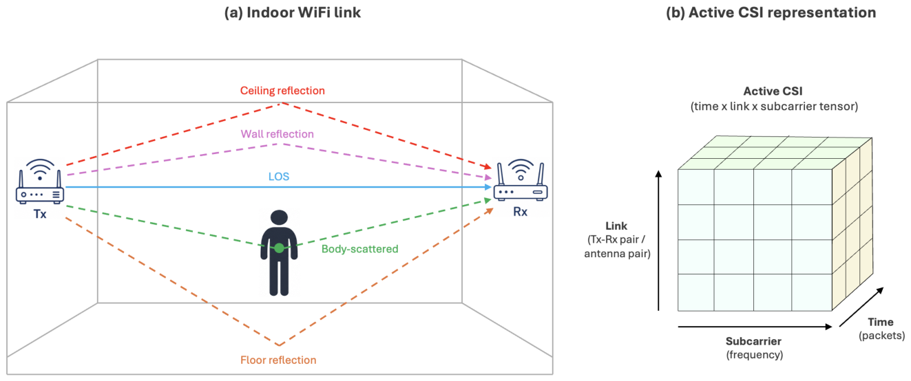
Figure 2.
Taxonomy of WiFi-based 3D reconstruction methods by reconstruction target and output representation. A matrix taxonomy with four reconstruction-target rows and six output-representation columns. Blank regions indicate target–representation combinations for which no method was identified in the surveyed literature. Note. † preprint or under review; * accepted or to appear; ‡ dense surface correspondence rather than an explicit metric 3D mesh; § partial spatial output rather than complete geometric reconstruction; ¶ primarily evaluated in 2D on the authors’ dataset, with explicit 3D results reported on MM-Fi. Publication status is reported as of July 2026.
Figure 2.
Taxonomy of WiFi-based 3D reconstruction methods by reconstruction target and output representation. A matrix taxonomy with four reconstruction-target rows and six output-representation columns. Blank regions indicate target–representation combinations for which no method was identified in the surveyed literature. Note. † preprint or under review; * accepted or to appear; ‡ dense surface correspondence rather than an explicit metric 3D mesh; § partial spatial output rather than complete geometric reconstruction; ¶ primarily evaluated in 2D on the authors’ dataset, with explicit 3D results reported on MM-Fi. Publication status is reported as of July 2026.
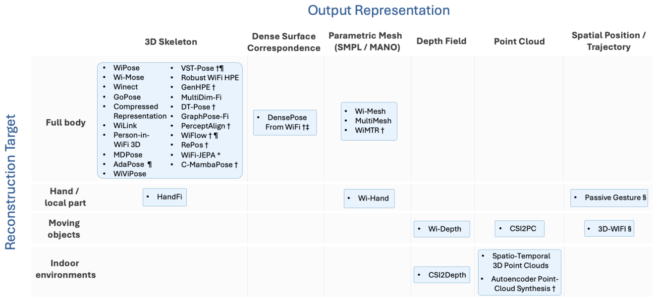
Figure 3.
Roles of reference annotations in WiFi-based 3D reconstruction. Reported prediction error usually measures agreement with an operational supervision or evaluation reference. Stronger geometric validation compares both the operational annotations and the WiFi prediction against an additional independent reference. A diagram showing measured WiFi entering a WiFi 3D reconstruction model and producing predicted geometry. One annotation source provides supervision and routine evaluation labels, while a separate geometric reference independently evaluates both those labels and the WiFi prediction. Note. Independence is determined by how a reference is used, not only by its sensing modality. A source used for training or routine evaluation is an operational reference; external validation requires an additional geometric reference not used by the reconstruction pipeline.
Figure 3.
Roles of reference annotations in WiFi-based 3D reconstruction. Reported prediction error usually measures agreement with an operational supervision or evaluation reference. Stronger geometric validation compares both the operational annotations and the WiFi prediction against an additional independent reference. A diagram showing measured WiFi entering a WiFi 3D reconstruction model and producing predicted geometry. One annotation source provides supervision and routine evaluation labels, while a separate geometric reference independently evaluates both those labels and the WiFi prediction. Note. Independence is determined by how a reference is used, not only by its sensing modality. A source used for training or routine evaluation is an operational reference; external validation requires an additional geometric reference not used by the reconstruction pipeline.
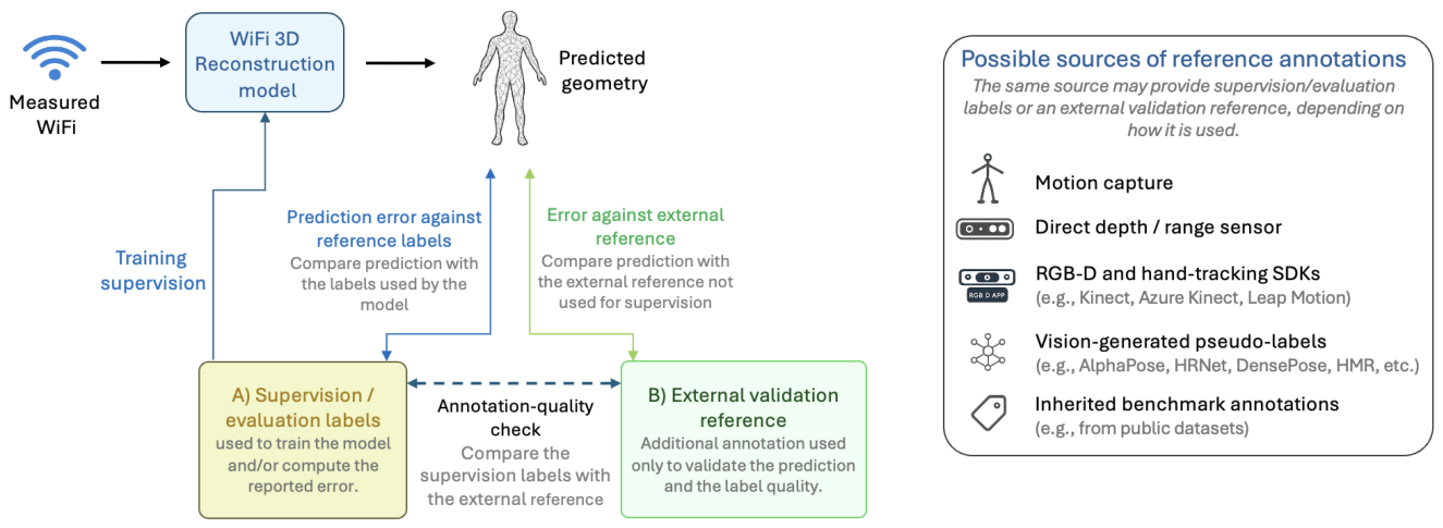
Figure 4.
Four lessons from vision and the maturity of their empirical validation in surveyed WiFi-based 3D reconstruction. A four-row synthesis of lessons from vision for WiFi-based 3D reconstruction. Each row contains an illustrative icon, a lesson, its implication for WiFi reconstruction, and five circles indicating the qualitative breadth and directness of empirical support. Structured output priors have four filled circles; observation consistency and identifiability has one; representation–architecture alignment has three; and acquisition- and domain-aware modelling has two. Note. More filled circles indicate broader and more direct empirical support for the stated implication in the surveyed literature. The indicators are qualitative and do not represent numerical scores or method rankings. For observation consistency, the low level reflects that the proposed prediction-to-WiFi mechanism remains unvalidated, although the review-wide finding that no such mechanism was identified is strong.
Figure 4.
Four lessons from vision and the maturity of their empirical validation in surveyed WiFi-based 3D reconstruction. A four-row synthesis of lessons from vision for WiFi-based 3D reconstruction. Each row contains an illustrative icon, a lesson, its implication for WiFi reconstruction, and five circles indicating the qualitative breadth and directness of empirical support. Structured output priors have four filled circles; observation consistency and identifiability has one; representation–architecture alignment has three; and acquisition- and domain-aware modelling has two. Note. More filled circles indicate broader and more direct empirical support for the stated implication in the surveyed literature. The indicators are qualitative and do not represent numerical scores or method rankings. For observation consistency, the low level reflects that the proposed prediction-to-WiFi mechanism remains unvalidated, although the review-wide finding that no such mechanism was identified is strong.
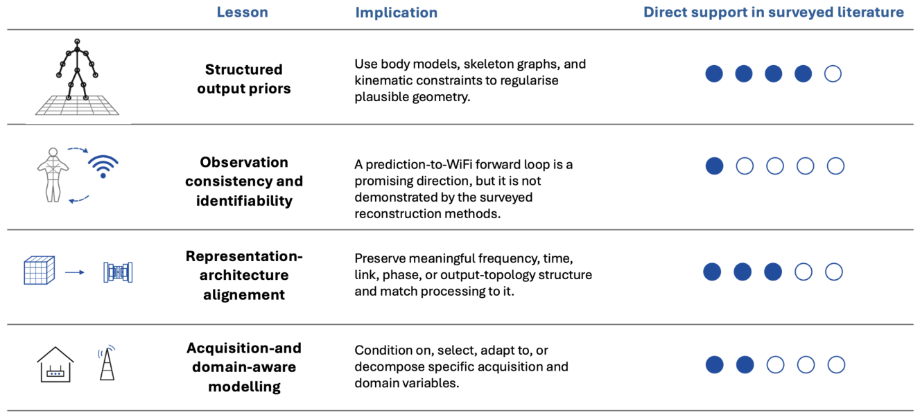

Table 1.
Coverage-based positioning of this survey relative to prior wireless and WiFi sensing surveys. Prior work provides complementary coverage of sensing applications, physical modelling, deep learning, skeleton reconstruction, reproducibility, or generalisability. The present survey differs by jointly covering multiple WiFi-derived 3D output representations, acquisition-aware comparison, vision-to-WiFi transfer, and output-specific evaluation and benchmark critique.
Table 1.
Coverage-based positioning of this survey relative to prior wireless and WiFi sensing surveys. Prior work provides complementary coverage of sensing applications, physical modelling, deep learning, skeleton reconstruction, reproducibility, or generalisability. The present survey differs by jointly covering multiple WiFi-derived 3D output representations, acquisition-aware comparison, vision-to-WiFi transfer, and output-specific evaluation and benchmark critique.
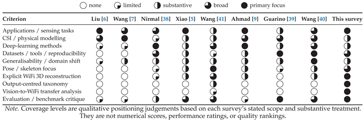 |
Table 2.
Survey protocol for identifying and selecting WiFi-based 3D reconstruction studies.
| Item | Protocol |
|---|---|
| Sources and seeds | Google Scholar, Semantic Scholar, IEEE Xplore, ACM Digital Library, arXiv, and SpringerLink, seeded by prior WiFi/RF surveys and MM-Fi [6,7,9,38,39,40,52]; last updated July 2026. |
| Search strings | Combinations of WiFi/CSI/RF with 3D pose, skeleton, mesh, SMPL, MANO, DensePose, depth, point cloud, trajectory, localisation, reconstruction, cross-domain, foundation model, differentiable ray tracing, and passive WiFi radar. |
| Screening | Title/abstract relevance; explicit 3D or geometry-proxy output; inference-time input derived from WiFi signals, including active CSI and passive WiFi radar observations. Methods whose primary inference-time input is millimetre-wave (mmWave) radar, ultra-wideband (UWB), radio-frequency identification (RFID), RGB imagery, LiDAR, or RSSI-only sensing are excluded from the main survey. |
| Inclusion/exclusion | Core methods output 3D skeletons, meshes, depth, point clouds, or geometry proxies from WiFi-derived input. Pure 2D pose, activity recognition, identity recognition, RSSI-only localisation, and non-WiFi sensing are related-only unless they clarify boundaries, supervision, or evaluation. |
| Borderline cases | DensePose From WiFi [25] is a surface-representation boundary case; 3D-WiFi [37] and Passive Gesture [36] are geometric proxies; WiFi point-cloud tracking [53] is related spatial-geometry work because its reported output is a 2D trajectory. |
| Study selection | Candidate papers identified through the stated search process were screened, and 34 WiFi-derived core, boundary, or proxy methods satisfying the inclusion criteria were included in the main analysis. These methods are organised jointly by reconstruction target and output representation and are summarised in separate skeleton and non-skeleton methodological comparison tables. |
Table 3.
Compact methodological comparison of WiFi-based 3D skeleton reconstruction methods.
| Method / target | Acquisition | WiFi representation | Supervision | Evaluation scope |
|---|---|---|---|---|
| WiPose [11] / body | Distributed commodity receivers | Complex CSI; derived 3D velocity profile | Vicon joints | Cross-subject, activity, room, furniture, occlusion, and antenna changes |
| Wi-Mose [56] / body | Two approximately orthogonal commodity links | Amplitude–phase CSI images | AlphaPose and VideoPose3D labels | Moving subjects; LOS/NLoS; cross-subject |
| Winect [12] / body | One transmitter, four receivers; L-shaped array | 2D AoA and path-length changes | Kinect 2.0 trajectories | Across days/environments; free-form activity; NLoS |
| GoPose [13] / body | One transmitter, four receivers; multi-link L-shaped arrays | Multi-link 2D-AoA profiles | Kinect 2.0 joints | Cross-subject/room; unseen activity; NLoS |
| Compressed Representation [57] / body | Commodity multi-antenna WiFi | Amplitude/phase and compressed heatmaps | Camera-generated skeletons | Two study-specific environments |
| WiLink [58] / body | Three Intel 5300 transmitters and three receivers; nine device links | Selected-link amplitude/phase in a fixed input layout | Camera/VideoPose3D joints | Held-out samples, unseen subject, position, and link-selection tests |
| Person-in-WiFi 3D [14] / multiple people | One transmitter and three multi-antenna receivers | Amplitude–phase CSI tokens | Azure Kinect skeletons | One–three people; leave-one-environment-out |
| MDPose [59] / body | Passive radar; synchronised reference/surveillance USRP channels | CLEAN-processed and denoised time–micro-Doppler | Mocap joints/velocities; SimHumalator | Seven subjects, three rooms, activities, and reduced-data tests |
| AdaPose [17] / body | TP-Link N750; two transceiver configurations; MM-Fi evaluation | Amplitude-only CSI windows | HRNet 2D pseudo-labels; MM-Fi 3D joints | Target-assisted cross-configuration adaptation; MM-Fi cross-room transfer |
| WiViPose [60] / body | Commodity WiFi with training-time video | Time/frequency and Doppler features | Video-derived pose | Cross-environment laboratory, gym, and bedroom tests |
| VST-Pose [61] / body | Commodity WiFi; MM-Fi evaluation | CSI amplitude sequences | OpenPose 2D; MM-Fi 3D joints | Authors’ 2D and MM-Fi 3D protocols |
| Robust WiFi HPE [62] / body | MM-Fi commodity configuration | Denoised, subcarrier-weighted CSI | MM-Fi joints | Random, cross-subject/environment, and added-noise tests |
| GenHPE [18] / body | PiW3D WiFi benchmark | Measured CSI; training-only generated full/part-removed RF | PiW3D joints | Random, repeated cross-subject, and cross-environment evaluation |
| MultiDim-Fi [63] / body | MM-Fi commodity configuration | Wavelet-filtered amplitude and unwrapped phase | MM-Fi joints | Reported MM-Fi protocol |
| DT-Pose [20] / body | PiW3D and MM-Fi configurations | Image-like antenna–subcarrier–time tensor; masked pretraining | Benchmark joints | In-domain, cross-subject, and cross-environment |
| GraphPose-Fi [21] / body | MM-Fi; one transmitter and three-antenna receiver | Antenna-pair–subcarrier–time tensor | MM-Fi joints | Random, cross-subject, and cross-environment |
| PerceptAlign [19] / body | Intel 5300; one transmitter, three receivers; varied layouts | Receiver magnitude/phase/Doppler plus calibrated geometry | EasyMocap joints | In-domain, cross-layout, cross-subject, and held-out scenes |
| WiFlow [64] / body | Commodity WiFi; MM-Fi evaluation | CSI amplitude sequences | OpenPose 2D; MM-Fi 3D joints | Continuous 2D and MM-Fi 3D evaluation |
| C-MambaPose [22] / body | MM-Fi commodity configuration | Sanitised unit-circle phase and amplitude | MM-Fi joints | MM-Fi random, cross-subject, and cross-environment settings |
| RePos [23] / body | PiW3D and MM-Fi commodity configurations | Body-part queries for relative pose; spatial heatmap for pelvis location | Benchmark joints | In-domain and MM-Fi cross-environment/few-shot protocols |
| WiFi-JEPA [24] / multiple people | PiW3D; real and ray-traced pretraining | Factored channel–time–link tokens with complete-link masking | Unlabelled pretraining; benchmark joints | Single/multi-person; leave-one-environment-out |
| HandFi [28] / hand | TP-Link/Atheros; one transmit and three receive antennas | Normalised real/imaginary CSI over streams, subcarriers, and packets | Leap joints; GrabCut masks | Unseen users/gestures, positions, rooms, distance, and occlusion |
Note. USRP denotes Universal Software Radio Peripheral; HRNet denotes High-Resolution Network; LOS and NLoS denote line-of-sight and non-line-of-sight conditions, respectively.
Table 4.
Compact comparison of WiFi-based reconstruction methods with non-skeleton outputs.
| Method / target | Acquisition | Representation | Supervision | Evaluation scope |
|---|---|---|---|---|
| Dense correspondence | ||||
| DensePose From WiFi [25] / people | antenna pairs; commodity CSI/video | Five-sample amplitude/phase windows translated to image-like features | DensePose/keypoint pseudo-labels and RGB teacher | Random split over 16 layouts; one held-out layout |
| Parametric meshes | ||||
| Wi-Mesh [26] / body | One 3-antenna transmitter; two custom 9-antenna receivers | Temporal azimuth–elevation spectra from 4D MUSIC | VIBE pose and VideoAvatar shape | Unseen subjects/environments, NLoS, clothing, distance |
| MultiMesh [16] / people | One 3-antenna transmitter; custom 9-antenna receiver | Per-person angular sequences after 4D propagation separation | Camera-derived SMPL references | Two/three people, unseen subjects/room, spacing and occlusion |
| WiMTR [15] / people | One transmitter; three 3-antenna Intel 5300 receivers | Amplitude–phase receiver–antenna–time tokens | Filtered ROMP SMPL pseudo-labels | Seven volunteers, one–four people, fixed split |
| Wi-Hand [29] / hand | One 3-antenna transmitter; custom 9-antenna receiver | Hand-specific angular sequences from 5D MUSIC | Camera-derived MANO pseudo-labels | Subject, environment, interference, occlusion, distance |
| Depth fields | ||||
| Wi-Depth [31] / object | Commodity WiFi plus training-time depth | Preprocessed CSI | Depth and auxiliary geometric labels | Shape, depth, position, and subject tests |
| CSI2Depth [32] / scene | MM-Fi commodity configuration | Spatiotemporal amplitude/phase | MM-Fi depth images | Cross-subject and cross-room |
| Point clouds | ||||
| CSI2PC [33] / object | Commodity testbed | CSI amplitude/phase | Paired object clouds | Study-specific objects/viewpoints |
| Määttä et al. [34] / scene | MM-Fi commodity configuration | Spatiotemporal CSI tokens | LiDAR-derived clouds | Unseen subjects/environments |
| Pannone–Avola [35] / environment | Paired ESP32 CSI/scene captures | CSI-to-point-cloud latent mapping | RGB/COLMAP clouds | Preliminary room protocol |
| Spatial outputs | ||||
| 3D-WiFi [37] / target | External L-shaped commodity array | Azimuth/elevation and equivalent arrival time | 3D coordinates | Two indoor localisation scenes |
| Passive Gesture [36] / hand | Two commodity links with linear arrays | Angles and path-length changes | Leap trajectories | Cross-user/environment tracking |
Note. MUSIC denotes multiple signal classification.
Table 5.
Principal reusable datasets and category-defining collections. Packet, frame, window, and sequence counts are omitted because the source papers report them in incompatible units.
Table 5.
Principal reusable datasets and category-defining collections. Packet, frame, window, and sequence counts are omitted because the source papers report them in incompatible units.
| Resource / output | Coverage | Acquisition | Reference labels | Split / shift | Public |
|---|---|---|---|---|---|
| WiPose [11] / skeleton | Controlled study | Distributed commodity receivers | Vicon joints | Subject/activity and deployment tests | NR |
| MDPose [59] / skeletal motion | 7 subjects; 3 rooms | Passive WiFi radar; synchronised USRP channels | Mocap joints/velocities; simulated Doppler | Predefined-layout subject/environment tests | NR |
| PiW3D [14] / skeleton | 7 subjects; 1–3 people; 3 scenes | One transmitter, three Intel 5300 receivers | Azure Kinect SDK joints | Official multi-person split; reused cross-environment | Yes |
| MM-Fi [52] / multimodal geometry | 40 subjects; 4 environments | TP-Link N750 plus synchronised modalities | Triangulated/refined camera keypoints and other modalities | S1 random, S2 subject, S3 environment | Yes |
| PerceptAlign [19] / skeleton | 21 participants; 5 scenes; 7 layouts | Intel 5300 with varied transceiver positions | EasyMocap multi-view joints | In-domain, cross-layout, held-out scenes | Yes |
| HandFi [28] / hand skeleton/mask | 6 subjects; 5 positions/rooms | TP-Link/Atheros plus Leap Motion | Leap joints; GrabCut masks | Random main split plus user/position/room tests | NR |
| DensePose From WiFi [25] / correspondence | 8 subjects; 1–5 people; 16 layouts | antenna pairs plus RGB | DensePose/keypoint pseudo-labels and teacher features | Random all-layout split; one held-out layout | NR |
| WiMTR [15] / multi-person mesh | 7 volunteers; 1–4 people; 3 scenes | Intel 5300 receivers plus Azure Kinect RGB | Manually filtered ROMP SMPL labels | Fixed split and crowd-size analysis | NR |
| Wi-Hand [29] / hand mesh | 3 environments; participant count unclear | Custom 9-antenna Intel 5300 array plus camera | Image-derived MANO labels | Subject, leave-one-subject-out, and held-out-environment tests | NR |
| Wi-Depth [31] / depth | 6 subjects; 4 environments | Intel 5300 plus depth sensor | Depth, mask, and centre labels | Leave-one-subject-out within each room | NR |
| Pannone–Avola [35] / scene cloud | 3 rooms | Two ESP32 devices | RGB/COLMAP point clouds | Study-specific room experiments | NR |
Note. “Public” denotes a reusable dataset release; NR means not reported in the reviewed source.
Table 6.
Output-specific evaluation: reported metrics, reporting conventions, and suggested diagnostic controls.
Table 6.
Output-specific evaluation: reported metrics, reporting conventions, and suggested diagnostic controls.
| Output | Principal metrics | Reporting conventions | Suggested controls / complementary reporting |
|---|---|---|---|
| 3D skeleton | MPJPE or Euclidean joint error; root-centred and PA-MPJPE separately; PCK; temporal error | Joint set, units, coordinate frame, root, person matching, alignment, aggregation, threshold | Absolute and aligned errors; no-CSI/constant, shuffled-CSI, temporal-only, nearest-neighbour, and per-joint/temporal breakdowns |
| Dense correspondence | Detection/keypoint average precision (AP); GPS/GPSm; combined dense scores | Atlas and visible-region policy, teacher version, threshold, body-part weighting, layout/subject/hardware changes | Held-out layout/environment, label-quality audit, no-CSI and shuffled-CSI controls; state that GPS is canonical rather than metric 3D |
| Parametric mesh | PVE/MPVPE; joint error; aligned vertex/joint error; PCK where used | Body-model version, vertex/joint mapping, units, root, scale, alignment, person matching, label fitting | Unaligned plus aligned metrics; output-prior or matched unconstrained baseline; no-CSI, shuffled-CSI, and independent mesh reference |
| Depth field | root mean square error (RMSE), relative error (REL), and absolute relative error (AbsRel), thresholds; occupancy/silhouette only as complementary | Depth range/units, resolution, valid mask, missing-frame policy, synchronisation, exclusions | Constant/mean depth, nearest neighbour, shuffled CSI, per-depth-range and temporal consistency |
| Point cloud | Unaligned Chamfer Distance; F-score/completeness; Earth Mover’s Distance (EMD) where feasible; aligned metrics separately | Point count, units, normalisation, registration, threshold, target extent, sampling | Mean/template and nearest-neighbour clouds, unaligned/aligned reporting, completeness, no-CSI and shuffled-CSI |
| Position / trajectory | Absolute position/trajectory error; relative and endpoint error; success thresholds | Reference frame, dimensionality, duration, sample rate, smoothing, geometry, threshold | Static/constant and temporal-only paths, shuffled CSI, per-axis and percentile/cumulative-distribution-function (CDF) reporting |
Table 7.
Consolidated lessons from vision and a cross-cutting evaluation requirement for WiFi-based 3D reconstruction. The table distinguishes reported evidence, supported conclusions, and unresolved claims.
Table 7.
Consolidated lessons from vision and a cross-cutting evaluation requirement for WiFi-based 3D reconstruction. The table distinguishes reported evidence, supported conclusions, and unresolved claims.
| Lesson / requirement | Evidence in the reviewed literature | Supported conclusion | What remains unproven | Empirical status in WiFi literature |
|---|---|---|---|---|
| Structured output priors | The 24-region DensePose atlas and SMPL/MANO models provide predefined surface structure across dense outputs, while graph-based decoders and kinematic losses structure skeletons. DensePose From WiFi, Wi-Mesh, MultiMesh, WiMTR, and Wi-Hand retain their canonical or parametric surface priors throughout their ablations; DT-Pose, GraphPose-Fi, and C-MambaPose compare structured skeletal decoders or losses, while HandFi reports a direct ablation of its combined bone-length and palmar-structure constraint package. | Predefined body models, skeletal connectivity, and kinematic constraints restrict the output space and can improve structured prediction within the evaluated systems. | A universal gain across targets or acquisitions; the contribution of SMPL/MANO relative to matched unconstrained mesh decoders; and whether plausible outputs depend sufficiently on sample-specific CSI. | Broad adoption with direct but method-specific ablations |
| Observation consistency and identifiability | The review did not identify a surveyed method using a task-level prediction-to-WiFi consistency loss. Self-supervised CSI pretraining, simulation, and generative augmentation are used for different purposes. | A task-level prediction-to-WiFi consistency mechanism was not identified in the surveyed reconstruction literature. A calibrated forward model or surrogate could add a compatibility constraint between predicted geometry and measured WiFi. | Whether it improves reconstruction or transfer; whether the model is accurate; whether geometry is identifiable; and whether the missing loop causes current domain failures. | Strong survey-wide finding; proposed mechanism remains unvalidated |
| Representation–architecture alignment | Methods use learned image-like translations, angle spectra, micro-Doppler, antenna–subcarrier–time tensors, channel–time–link tokens, complex features, and graph decoders. DensePose From WiFi ablates phase and teacher supervision; HandFi compares complex-signal embedding, dense mask supervision, and mask losses; MDPose compares measured and simulation-assisted denoised micro-Doppler pathways; Wi-Mesh, MultiMesh, and Wi-Hand compare propagation-derived inputs; Wi-Hand also ablates feature injection and temporal processing; WiMTR compares phase processing, refinement, and query generation; and WiFi-JEPA, C-MambaPose, and GraphPose-Fi report tokenisation, complex-processing, or aggregation comparisons. | Preserving relevant frequency, time, antenna, link, phase, or output topology and matching processing components to that structure can improve performance within an evaluated system. | A universal ranking of representations or architectures and transfer of reported gains across hardware, link layouts, bandwidths, or outputs. | Moderate, mainly within-system evidence |
| Acquisition- and domain-aware modelling | PerceptAlign conditions on calibrated transceiver geometry, WiLink selects signal-informative links, MultiMesh ablates calibration and static reflection suppression, AdaPose uses target CSI for adaptation, HandFi aligns source-position latent covariances for held-out-position generalisation, GenHPE applies training-only skeleton-conditioned counterfactual regularisation, and RePos separates pelvis-relative structure from absolute pelvis localisation. | Specific acquisition or domain variables can be exposed through conditioning, selection, adaptation, regularisation, or output decomposition. | A unified decomposition of pose, shape, environment, layout, calibration, and hardware; statistical independence; and cross-device robustness. | Emerging, system-specific evidence across heterogeneous protocols |
| Cross-cutting evaluation requirement | Reference geometry ranges from motion capture and measured depth to RGB-D SDK estimates and vision pseudo-labels. Output types use incompatible metrics, alignments, and coordinate conventions, while signal-use controls are rarely reported. | Evaluation should distinguish dependence on measured CSI, agreement with the label-generation pipeline, and accuracy against an independent geometric reference. | A common benchmark spanning all output and acquisition classes and routine availability of independent geometric references. | Strong methodological rationale; limited current adoption |
Note. The final column describes the maturity of empirical validation of each row’s WiFi-specific implication, not the importance or validity of the underlying lesson or requirement. It considers breadth of adoption, directness of testing, and experimental control. Effect sizes from different datasets, acquisition configurations, output representations, alignments, or metrics are not compared across rows.
Disclaimer/Publisher’s Note: The statements, opinions and data contained in all publications are solely those of the individual author(s) and contributor(s) and not of MDPI and/or the editor(s). MDPI and/or the editor(s) disclaim responsibility for any injury to people or property resulting from any ideas, methods, instructions or products referred to in the content. |
© 2026 by the authors. Licensee MDPI, Basel, Switzerland. This article is an open access article distributed under the terms and conditions of the Creative Commons Attribution (CC BY) license (http://creativecommons.org/licenses/by/4.0/).
Copyright: This open access article is published under a Creative Commons CC BY 4.0 license, which permit the free download, distribution, and reuse, provided that the author and preprint are cited in any reuse.