

Submitted:
28 August 2026
Posted:
31 August 2026
You are already at the latest version
Abstract
European packaging policy is built almost entirely around treatment, while the prevention obligation that accompanies it lacks an equivalent apparatus of measurable objectives. This article addresses the upstream question directly, asking what determines the quantity of plastic packaging waste that European economies place on the market. Plastic packaging waste generated per capita, from Eurostat, is regressed on the environmental, social and governance pillars of the World Bank Sovereign ESG framework for twenty-nine countries between 2014 and 2023. Each pillar is examined through three modules: a panel comparison of pooled, between, fixed effects, random effects, weighted and dynamic estimators, with inference re-assessed by wild cluster bootstrap; an unsupervised classification comparing six algorithms across eleven validity indices, with the dependent variable withheld for external validation; and a supervised comparison of six learners under leave-country-out cross-validation, used to validate functional form rather than to forecast. Three findings emerge. Energy intensity and carbon intensity per capita are robustly associated with generation and survive correction for multiple testing, yet environmental country types carry no information about packaging burden. Social configurations do separate generation, along a binary post-transition boundary, and the sign reversal on life expectancy between the cross-sectional and time dimensions is confirmed independently by the learners. Internet penetration is the strongest association in the study, while composite institutional quality is insignificant in every linear specification and emerges under unrestricted functional form as a threshold rather than a gradient. Prevention policy must therefore engage determinants that lie outside waste management, of which online retail is currently the most important.
Keywords:
plastic packaging waste
; waste prevention
; ESG indicators
; panel data
; machine learning
; extended producer responsibility
; e-commerce
; European Union
1. Introduction
Plastic packaging is the material fraction on which European waste policy has most visibly failed. Paper, glass and metal approach saturation, with recycling rates above eighty per cent in most member states, while the plastic fraction remains below forty per cent and has improved by barely one percentage point in a decade. The policy response has been almost entirely downstream: recycling targets, producer responsibility schemes, deposit-return systems and, most recently, a regulation replacing the packaging directive. The prevention obligation in European waste law has never acquired an equivalent apparatus of measurable objectives, and the quantity of plastic packaging entering the system each year has attracted correspondingly less attention than what happens to it afterwards.
The asymmetry is reproduced in the research literature. The determinants of waste generation have been studied extensively but almost exclusively for the municipal aggregate, from early decoupling assessments to recent panel analyses of European and OECD economies. The packaging literature has concentrated instead on policy design, material flows and end-of-life performance, treating the quantity generated as a denominator rather than as something to be explained. The closest antecedent examining packaging generation as a dependent variable in a cross-country panel remains Mazzanti and Nicolli (2011), restricted to the EU15, concerned with decoupling rather than with a structured set of determinants, and now fourteen years old.
This article addresses that question directly: what accounts for cross-country and over-time variation in plastic packaging waste generated per capita in Europe, and through which of the environmental, social and governance dimensions of national performance does that variation operate?
Three gaps in the existing literature motivate the design.
The first concerns the outcome. Plastic packaging generation has not been treated as a dependent variable in a cross-country econometric analysis, despite being the stream on which European targets have most conspicuously failed. Using generation rather than the recycling rate reverses the conventional choice deliberately: treatment outcomes are the product of collection infrastructure and producer responsibility arrangements, that is, of institutions, whereas generation measures how much packaging material passes through an economy and is therefore the quantity to which structural country characteristics can plausibly be related.
The second concerns the organisation of the determinants. Studies select explanatory variables pragmatically, so the relative contribution of environmental, social and institutional conditions cannot be compared across them. This article adopts the pillar structure of the World Bank Sovereign ESG framework, which is external to the analysis and therefore not selected to produce results, and estimates three equations sharing one dependent variable. The framework has been applied overwhelmingly at firm level, and its country-level application to a waste outcome is, to our knowledge, new.
The third concerns method. Panel econometrics, unsupervised classification and supervised learning are applied in this field in separate literatures, and where they have been combined the algorithmic component serves description rather than validation. Here the third module is designed explicitly to test whether the linear panel specification survives comparison with algorithms free to fit interactions and thresholds on the same information, and whether permutation importance recovers the same variable hierarchy as the econometric estimates. The clustering module is designed symmetrically: the dependent variable is withheld from the classification space and reserved for external validation, so that any association between country types and packaging burden is recovered rather than imposed.
The design yields three substantive results and one methodological one. Energy and carbon intensity are robustly associated with generation and survive correction for multiple testing, yet environmental country types carry no information about packaging burden. Social configurations do separate generation, along a boundary coinciding with the post-transition divide. The diffusion of online retail is the strongest single association in the study, a mechanism the e-commerce literature has described qualitatively but never estimated on a generation outcome. Methodologically, composite institutional quality is insignificant in every linear specification yet emerges under unrestricted functional form as a threshold rather than a gradient.
2. Literature Review
The question of whether waste generation can be separated from economic growth has organised this literature for two decades, and it supplies the analytical frame within which the present article situates its dependent variable. The reference model is the waste Kuznets curve, which posits an inverted-U relationship between income and waste per capita, with a turning point beyond which further growth reduces material throughput. Evidence for the European Union has been mixed from the outset. Mazzanti and Nicolli (2011) examined municipal and packaging waste generation jointly for the EU15 and found only partial decoupling, with packaging waste behaving differently from the municipal aggregate — an early indication that the two streams should not be treated interchangeably. Arbulú et al. (2015), in the most cited contribution of this strand, assessed the effect of tourism volume, quality and specialisation on municipal solid waste generation in a European panel and confirmed the Kuznets specification while identifying tourism as a distinct generator that income alone does not capture.
Subsequent work has both extended the geography and questioned the functional form. İçen and Çil (2023) estimated the municipal waste Kuznets curve for 22 OECD countries over 1995–2018, incorporating human capital, material footprint, consumption and urban population alongside income. Koçak and Bağlıtaş (2022) confirmed the inverted-U for OECD countries between 2003 and 2018 using both static and dynamic panel methods, and located the turning point at an income level beyond which technological and human-development effects dominate. Mazzarano et al. (2021) challenged the standard specification directly, arguing that income elasticities of waste generation are not constant and that testing a single alternative hypothesis against the linear case is insufficient. Chakraborty et al. (2022) reached a related conclusion for Italy, showing that decoupling has not arisen homogeneously across regions or over time, and that breaks and thresholds are required to represent the waste–income relationship. The most recent contributions continue to find the question open: Ahmed et al. (2026) ask whether economic growth still drives municipal waste in the European Union and the Western Balkans, and Guler et al. (2025) introduce inflation instability as a determinant of municipal waste generation across thirty European countries between 1995 and 2021.
Methodologically, this strand has converged on panel estimators with explicit treatment of cross-sectional dependence. Sinha et al. (2022) applied a common correlated effects framework to solid waste generation in the OECD, and Akther et al. (2025) estimated a STIRPAT specification for 33 European countries over 1995–2021 with corrections for cross-sectional dependence, including gross domestic product, research and development expenditure, tourism, trade volume, renewable energy adoption and the growth of the service sector. Gardiner and Hájek (2020) examined the joint dynamics of municipal waste generation, research intensity and growth at the level of European regions, and Shah et al. (2023) added industrialisation and foreign direct investment for OECD economies over 2000–2020.
Socio-demographic and structural determinants. A second strand asks which country characteristics, beyond income, account for differences in the quantity of waste generated. Hondroyiannis et al. (2024a) estimated short- and long-run responses of municipal waste generation to socio-economic and demographic variables at both national and regional level in Europe, comparing pooled ordinary least squares, fixed effects and random effects — the same estimator comparison adopted in the present article. The companion study by the same group (Hondroyiannis et al., 2024b) applied the design to recycling rates and grouped the explanatory variables into socio-demographic, economic and structural sets, an organisational choice close in spirit to the pillar decomposition used here.
Work at sub-national level has documented the demographic mechanisms more directly. Rybová et al. (2018) analysed socio-demographic determinants of municipal waste generation across Czech municipalities and linked variation in household composition and behaviour to differences in generation rates. Antczak (2019) applied geographically weighted regression to Polish districts, identifying population density, the share of working-age population, wages and tourist presence among the significant determinants, and showing that the coefficients vary spatially rather than holding uniformly. Chalak et al. (2016) extended the analysis to 44 countries at different income levels and, importantly for the present article, found that legislation and regulation enter the explanation of household waste generation alongside economic variables.
The efficiency literature provides a complementary reading. Pais-Magalhães et al. (2021) scored the eco-efficiency of European waste sectors using data envelopment analysis, and lo Storto (2025) assessed 5,516 Italian municipalities, documenting persistent regional disparities in performance and cost that income alone does not explain. Osińska (2024) evaluated management efficiency across 23 EU member states before and after Directive (EU) 2018/851, and Malek et al. (2023) provided one of the few empirical evaluations of waste policy effects on the composition of treatment flows, using a panel of fourteen European countries.
Packaging as a distinct waste stream. Packaging has been studied predominantly as a policy object rather than as a quantity to be explained, and this asymmetry is the principal gap the present article addresses. The dominant framework is extended producer responsibility. Joltreau (2022) analysed whether producer responsibility schemes induce genuine packaging reduction and eco-design or merely finance end-of-life management, concluding that the incentive to reduce material at source is weaker than the incentive to recycle it. Colelli et al. (2022) assessed the effectiveness and efficiency of European packaging waste systems through both indicator-based comparison of producer responsibility organisations and regression analysis of national recycling rates. Rubio et al. (2019) examined the Portuguese case and Picuno et al. (2021) compared the plastic packaging recycling systems of Austria, Germany and the Netherlands, showing that schemes sharing a common legal basis diverge substantially in architecture and outcome. Ross et al. (2024) documented divergence of a different kind, in the French and German transposition of the same European provisions.
Deposit-return systems have attracted recent attention as a targeted instrument. Nikolić and Rotar (2026) estimated a panel regression of deposit-refund system effectiveness across EU countries, and Piontek et al. (2024) assessed whether such systems can deliver the separate collection and recycling objectives of the single-use plastics directive. Magrini et al. (2020) reviewed market-based instruments for municipal waste prevention in six member states, adopting a strict definition of prevention that excludes recycling and therefore aligns with generation rather than treatment as the outcome of interest.
Material flow accounting supplies the quantitative description of the stream. Cimpan et al. (2021) constructed plastic packaging flows for Europe through a hybrid input–output approach and subsequently assessed the effects of circularity interventions in the sector (Cimpan et al., 2023). Lombardi et al. (2021) performed a material flow analysis of Italian plastic packaging management, Lopez-Aguilar et al. (2022) did so for Spain while documenting substantial data gaps, and Jylhä et al. (2025) proposed a revised accounting method for plastic packaging waste, motivated by inconsistencies in reported figures. Robaina et al. (2020) ranked European countries by efficiency in the end-of-life treatment of plastics, and Winterstetter et al. (2022) produced country-specific estimates of mismanaged plastic packaging waste. Pavón Losada et al. (2025) report that food packaging alone accounts for 40.5% of European plastic production while only 35% of that waste is recycled, which quantifies the policy relevance of the stream.
What this body of work does not contain is a cross-country econometric explanation of how much plastic packaging is generated. Mazzanti and Nicolli (2011) remains the closest antecedent, and it is fourteen years old, restricted to the EU15 and concerned with decoupling rather than with a structured set of determinants.
Digitalisation and e-commerce. A small and recent literature connects the diffusion of digital commerce to packaging demand, and it is directly relevant to the strongest empirical result reported below. Khatami et al. (2023) examined the joint role of consumer behaviour and the digital ecosystem in plastic waste generation, treating digitalisation as a driver rather than as a management tool. Tyagi et al. (2021) identify the rapid growth of e-commerce and fresh-food preservation as the market dynamics shaping food packaging technology, noting that the sector accounts for over 40% of plastic waste. Clement and Spinler (2025) modelled reusable packaging systems for e-commerce and quantified the environmental and financial trade-offs, while Doran et al. (2025) estimated the relationship between e-commerce activity and climate outcomes in EU countries using panel quantile methods. The complementary literature treats digitalisation as an instrument of waste management rather than a source of waste. Sarc et al. (2019) surveyed digitalisation and intelligent robotics across the circular economy value chain, D’Adamo et al. (2022) related waste policy to circular economy goals in a setting where digitalisation supports industrial sectors, and Bassem (2026) estimated nonlinear and dynamic effects of digitalisation on waste-to-energy development in the European Union. The two readings are not in conflict, but they have not been tested against one another on a generation outcome, and the sign of the net association remains an open empirical question.
Machine learning and clustering in cross-country waste research. Algorithmic methods entered this field first as forecasting tools. Antanasijević et al. (2013) modelled municipal waste generation with artificial neural networks and generic sustainability indicators for countries at different development levels, and Oguz-Ekim (2021) compared three machine learning algorithms for generation forecasting. Rosecký et al. (2021) developed predictive models across territorial levels to support treatment capacity planning, and Szul et al. (2026) evaluated six feature-selection methods against five predictive techniques for 79 Slovak districts using 45 socio-economic and demographic variables. Chen and Chang (2024) combined circular economy metrics with gradient boosting and Shapley additive explanations for EU municipal waste over 2010–2020, which is among the few applications that use algorithmic output for interpretation rather than prediction alone.
Two studies come closest to the design adopted here. Smailbegović et al. (2025) analysed the determinants of municipal solid waste generation treating Europe as a single unit rather than as a collection of regional case studies, using machine learning to identify socio-economic, demographic and environmental drivers. Cehlár et al. (2025) combined determinant analysis with country profiling for EU municipal waste recycling over 2005–2023, explicitly pairing econometric estimation with a grouping exercise. Clustering has otherwise been used to characterise circular economy positions: Nademi and Sedaghat Kalmarzi (2025) applied spectral clustering to identify three groups of European countries in the circular economy and unemployment nexus before estimating panel models, Bodislav et al. (2025) clustered approaches to the trade-off between circularity and growth, and Morelli et al. (2024) applied deep learning to circular economy and entrepreneurship in the EU-27.
Country-level ESG frameworks and the contribution of this article. The environmental, social and governance framework has been applied overwhelmingly at firm level. Oyewo et al. (2024) is representative in relating board composition and ESG-linked compensation to industrial wastewater recycling, and Zein (2026) observes explicitly that existing evaluation frameworks for waste-to-hydrogen operate at the level of corporate reporting rather than at system level. Applications to countries remain scarce and indirect. Antanasijević et al. (2013) used generic sustainability indicators as predictors without organising them into pillars; Vučkovski et al. (2025) selected environmental protection indicators, including the recycling rates of municipal and packaging waste, to explain growth sustainability across 21 member states over 2013–2022; and Streimikis (2026) compared circularity performance in the Benelux economies through material footprint and waste generation per capita. Vardopoulos et al. (2021) and Avilés-Palacios and Rodríguez-Olalla (2021) frame waste management within sustainability assessment but without an estimation strategy.
Three gaps follow from this review, and the present article addresses each. First, plastic packaging generation has not been treated as a dependent variable in a cross-country panel, despite being the stream on which European targets have most conspicuously failed. Second, the three ESG pillars have not been used as a structured partition of the determinant space, so that the relative contribution of environmental, social and governance conditions cannot be compared on a common outcome. Third, the econometric, clustering and machine learning approaches surveyed above are applied in separate literatures; where they have been combined, as in Cehlár et al. (2025), the algorithmic component serves description rather than validation of the econometric specification. The design adopted here uses the third module explicitly to test whether the linear panel specification survives comparison with unrestricted learners on the same information set.
3. Data and Methodology
The analysis combines two sources at the country-year level. The dependent variable comes from Eurostat’s packaging waste collection (env_waspac), which reports quantities generated and treated by material fraction under Directive 94/62/EC. The series begins in 2014; earlier observations were discontinued when reporting methodology was revised and are not comparable. Plastic packaging generated per capita was retained and logarithmically transformed, since the raw distribution runs from 11.7 to 73.0 kilograms per inhabitant and is right-skewed.
Explanatory variables come from the World Bank ESG Data Framework, which classifies seventy-eight country indicators into environmental, social and governance pillars and so supplies the partition of the determinant space directly, without an ad hoc assignment. Merging is on ISO3 code and year. Sixty-one indicators exceed eighty per cent coverage on the European sample and were retained; the rest are built for developing economies and are largely empty here.
The scope is the EU-27 plus Iceland, Liechtenstein and Norway, the thirty reporting entities of the collection. Liechtenstein drops out everywhere for absence of ESG coverage, Iceland also from the environmental block for absence of energy statistics. The environmental equation therefore rests on 28 countries and 243 observations over 2014–2022, the social and governance equations on 29 countries and 270 and 282 observations over 2014–2023. The panels are unbalanced, with four to ten annual observations per country and Cyprus at the lower bound. Windows differ because coverage differs; no common-sample restriction was imposed, since it would cost some fifteen per cent of the observations without altering a single coefficient sign.
All variables were winsorised at the first and ninety-ninth percentiles, and no retained specification exceeds a variance inflation factor of five. Each variable’s total variation was decomposed into between-country and within-country components, a step reported alongside the estimates because it determines what the within estimator can identify: two environmental indicators move so little inside countries that their fixed-effects estimates are not interpretable, and this is stated where it applies.
Each pillar is analysed through three modules applied to the same dependent variable. The first is panel estimation. Six estimators are reported side by side — pooled ordinary least squares, between, fixed effects, random effects, weighted least squares with population weights, and a dynamic least squares dummy variable specification — so that the between and within dimensions are compared rather than collapsed. Standard errors are clustered by country. Because twenty-nine clusters place cluster-robust inference near the limit of its asymptotic justification, every focal coefficient is re-assessed by a wild cluster bootstrap-t with Rademacher weights and the null imposed, on 1,999 replications, and against a Bonferroni threshold. Specification choice rests on the F test for individual effects, the Breusch–Pagan Lagrange multiplier test and a Mundlak correlated random effects formulation, which replaces the classical Hausman statistic because the latter is not computable under cluster-robust covariance. Cross-sectional dependence, serial correlation and heteroskedasticity are tested by the Pesaran CD, Wooldridge and Breusch–Pagan statistics.
The second module is unsupervised classification of country means. Six algorithms — K-Means, Ward agglomeration, a Gaussian mixture, Fuzzy C-Means, DBSCAN and proximity clustering from an unsupervised random forest — are compared on eleven validity indices, among them explained variance, silhouette, Dunn, Calinski–Harabasz, entropy and the Herfindahl–Hirschman index, and ranked by mean rank. The dependent variable is excluded from the classification space and reserved for external validation, so that any association between country types and packaging generation is found rather than imposed.
The third module compares six supervised learners — linear regression, linear support vector regression, k-nearest neighbours, a decision tree, a random forest and gradient boosting — under ten-fold cross-validation grouped by country, so that no country appears in both training and test partitions. Its purpose is validation, not forecasting: it asks whether the linear specification survives comparison with algorithms free to fit interactions and thresholds, and whether permutation importance recovers the same variable hierarchy as the econometric estimates. See Figure 1.
4. Panel Analysis: The Environmental Component
The dependent variable is the natural logarithm of plastic packaging waste generated per capita, from Eurostat (env_waspac). Plastic is chosen among the packaging fractions because it is the material for which European recovery targets have proved hardest to meet and because its generation is the least distorted by cross-border flows; the logarithmic form is dictated by the skewness of the raw series, which ranges from 11.7 to 73.0 kilograms per capita.
Generation rather than treatment is the appropriate dependent variable for the environmental pillar. Treatment outcomes are the product of collection infrastructure, sorting capacity and producer responsibility schemes, that is, of institutions. Generation measures how much packaging material passes through an economy, and is therefore a question about the metabolism of the production system, which is what the environmental indicators describe.
The regressors are taken from the World Bank ESG Data Framework: log population density, energy intensity of primary energy, carbon dioxide emissions per capita, net energy imports as a share of energy use, forest area as a share of land, and protected areas as a share of territory. Emissions and energy enter per capita or per unit of output rather than in levels, so that country size does not enter the specification twice. Variance inflation factors range from 1.30 to 4.99, and no pairwise correlation exceeds 0.70 in absolute value.
The estimation sample covers 28 countries between 2014 and 2022, for 243 observations, unbalanced between four and nine years per country. Figure 1 reports the distribution of the dependent variable in its original units. See Figure 2.
Table 1 reports six estimators over the same sample, with standard errors clustered by country in parentheses.
The most important feature of the table is the agreement across estimators. Explained variance is 0.455 in the pooled specification, 0.465 in the between dimension, 0.451 with fixed effects and 0.413 with random effects. The environmental block therefore accounts for a comparable share of the differences between countries and of the movements within them, which is unusual in macro panels of this size and indicates that the association is structural rather than an artefact of one dimension. Two regressors carry the result and do so consistently. Energy intensity is negative and significant in five of the six columns, with a fixed-effects elasticity of −0.414: a one-unit fall in megajoules per dollar of output is associated with a 41% rise in plastic packaging generated per capita. Carbon dioxide per capita is positive and significant in four columns, at 0.089 under fixed effects. Figure 2 places all estimators on a common standardised scale. See Figure 3.
Table 2 reports the tests that discriminate among estimators and characterise the error structure.
Pooling is rejected and country effects are present. The classical Hausman statistic is not reported because under cluster-robust covariance the difference of the two variance matrices is not positive semi-definite and the quadratic form turns negative, a well-known failure of the test in this setting; the Mundlak formulation, which is robust to it, rejects equality of the within and between coefficients at the 1% level. Fixed effects is therefore the specification to interpret, although the closeness of the estimates across columns means the choice matters less here than it usually does.
The errors are cross-sectionally dependent, serially correlated and heteroskedastic. Clustering addresses the last two. For the first, Appendix A4 re-estimates the model with Driscoll–Kraay standard errors, under which energy intensity, carbon intensity, density and protected areas remain significant at the 1% level.
With 28 clusters the asymptotic approximation underlying cluster-robust inference is imperfect, so the significance of Table 1 was re-assessed by a wild cluster bootstrap-t with Rademacher weights and the null imposed, on 1,999 replications. Energy intensity and carbon intensity return bootstrap p-values of 0.0005, which survive a Bonferroni correction over the six coefficients; the remaining four fall between 0.06 and 0.64. Figure 4 explains that pattern.
Population density and forest area have within shares of 2.3% and 1.2% of their total variation, so their fixed-effects coefficients are estimated on almost no information and should not be interpreted, notwithstanding the nominal significance of the latter in the dynamic column. The two variables that survive the bootstrap are precisely those with substantial within variation, at 21.9% and 23.6%.
A natural objection is that energy intensity, carbon intensity and packaging generation are all manifestations of economic development. Appendix A5 adds the logarithm of GDP per capita to the fixed-effects specification. Its own coefficient is 0.316 and significant at the 1% level, explained variance rises to 0.505, and the two focal coefficients survive at −0.289 and 0.072, both with p below 0.001. The association is therefore not a proxy for income.
Packaging generation is persistent, since it reflects consumption patterns and retail structures that change slowly. The autoregressive coefficient of 0.691 in the last column of Table 1 implies that about 31% of the gap from equilibrium closes each year and that long-run responses are 3.24 times the immediate impact.

Table 3.
Short-run and long-run effects from the dynamic environmental specification.
| Variable | Short run | Long run |
|---|---|---|
| Population density (log) | −0.2965 | −0.9606 |
| Energy intensity | −0.1091 | −0.3536 |
| CO2 per capita | 0.0224 | 0.0725 |
| Net energy imports | −0.0002 | −0.0005 |
| Forest area | −0.0320** | −0.1038 |
| Protected areas | 0.0011 | 0.0034 |
Note. Long-run effects computed as β/(1−ρ) with ρ = 0.6913. N = 215, R2 = 0.652.
The long-run coefficients on energy and carbon intensity, at −0.354 and 0.073, are close to the static fixed-effects estimates of −0.414 and 0.089. Since the least squares dummy variable estimator is biased downward in short panels, the persistence reported here is a lower bound. The Anderson–Hsiao alternative is reported in Appendix A6 and is not used for inference.
The environmental pillar explains close to half of the variation in plastic packaging generation, and does so equally well across countries and over time. The mechanism is legible: economies that use less energy per unit of output and emit less carbon per head place less plastic packaging on the market. Both associations survive the inclusion of income, so they are not restatements of development.
Two qualifications apply. The specification contains no time effects, so shocks common to all countries are not absorbed. And the design identifies structural associations rather than causal effects, since none of the regressors can be treated as exogenous to the material intensity of an economy. The natural complement is the treatment side: what a country does with the plastic it generates is governed by collection and producer responsibility arrangements, which is the subject of the governance equation.
5. Cluster Analysis of the Environmental Component
The panel estimates of Section 4 identify partial effects, that is, the association of each environmental indicator with plastic packaging generation holding the others constant. A complementary question is whether European economies fall into distinct environmental types, and whether membership of a type carries information about how much plastic packaging a country places on the market. This section addresses that question by unsupervised classification.
The units are the 28 countries of the estimation sample, described by the six environmental indicators averaged over 2014–2022 and standardised to zero mean and unit variance. All variables are winsorised at the first and ninety-ninth percentiles before averaging, which prevents Norway, a net energy exporter with an extreme value of net energy imports, from forming a singleton cluster. The dependent variable is deliberately excluded from the clustering space and reserved for external validation, so that any association recovered between types and packaging generation is not built in by construction.
Six algorithms were estimated at three clusters: K-Means, hierarchical agglomeration with Ward linkage, model-based classification through a Gaussian mixture with unrestricted covariances, Fuzzy C-Means with a fuzzifier of two, density-based classification through DBSCAN, and a proximity-based classification obtained from an unsupervised random forest of one thousand trees against a synthetic reference distribution. Table 4 reports eleven validity indices for each.
The DBSCAN figures are not comparable with the others and are excluded from the ranking. Its apparently superior fit is an artefact of coverage: by discarding almost half the sample as noise it computes every index on the fifteen most compact observations. With 28 units and no dense regions in a six-dimensional space, density-based classification is not an appropriate method here, and this is the substantive finding rather than a defect of implementation.
Ranking the five comparable algorithms on each index and averaging the ranks yields the ordering in Figure 5.
Hierarchical agglomeration with Ward linkage obtains the best mean rank at 2.23, narrowly ahead of K-Means at 2.32. The two are close on internal cohesion, with R2 of 0.422 against 0.426 and Calinski–Harabasz of 9.13 against 9.26, but Ward separates the groups substantially better: minimum separation is 1.302 against 0.903 and the Dunn index 0.232 against 0.161. Since the two methods agree on cohesion and differ on separation, the criterion that discriminates is the one on which Ward is superior. The Gaussian mixture attains the highest silhouette of the comparable set at 0.338, but it does so by producing a strongly unbalanced partition, with a Herfindahl–Hirschman index of 0.696 against 0.375 for Ward and an entropy of 0.559 against 1.032. Random forest proximity ranks last on nine of the eleven indices.
Ward linkage is therefore retained. Its cophenetic correlation of 0.594 indicates that the dendrogram represents the original distances only moderately well, which is expected with a small sample in six dimensions and is reported as a caveat rather than as support. Figure 6 shows the selection of the number of clusters.
The within sum of squares falls from 128.0 at two clusters to 97.1 at three and 76.5 at four, so the largest single reduction, 30.9, occurs at the third cluster and the increment declines thereafter. Silhouette is highest at two clusters, at 0.332, but that partition isolates five countries against twenty-three and conveys little. Davies–Bouldin and Calinski–Harabasz continue to improve up to eight clusters, which with 28 units would leave fewer than four observations per group and is not interpretable. Three clusters is retained as the point at which the elbow criterion, the balance of group sizes and interpretability coincide.
The partition assigns five countries to the first cluster, ten to the second and thirteen to the third. Table 5 reports the profiles in standardised units, so that each entry is the distance of the cluster average from the sample average in standard deviations.
The first cluster contains Estonia, Finland, Latvia, Norway and Sweden. It is defined by low population density at 1.52 standard deviations below the mean, extensive forest cover at 1.36 above, and energy self-sufficiency, with net energy imports one standard deviation below average. Energy intensity is high, which reflects the combination of a cold climate and resource-based industry rather than inefficiency in the ordinary sense.
The second cluster comprises Austria, Belgium, Bulgaria, Czechia, Germany, Luxembourg, the Netherlands, Poland, the Slovak Republic and Slovenia. Its signature is carbon intensity at 0.69 above the mean combined with the highest share of protected territory at 0.99, a combination of industrial emissions and formal conservation that characterises the continental core.
The third and largest cluster gathers the Mediterranean and western periphery, from Croatia, Cyprus and Greece to France, Ireland, Italy, Portugal, Spain and Romania. It is defined negatively: below-average energy intensity at −0.64, below-average carbon intensity at −0.64, limited forest cover and the highest dependence on imported energy. Its internal cohesion is the strongest of the three, with an average silhouette of 0.357 against 0.206 for the second cluster and 0.028 for the first. Figure 7 shows the partition in the plane of the first two principal components, which together account for 67.4% of the variance.
The first component, at 42.9% of the variance, opposes densely populated countries with imported energy to sparsely populated, forested and energy-intensive ones; the second, at 24.5%, captures carbon intensity and conservation effort jointly.
The decisive test is whether the three environmental types differ in plastic packaging generation, the variable withheld from the classification. They do not. Cluster averages of the logarithm of generation per capita are 3.412, 3.347 and 3.402, and the differences are not significant by either analysis of variance, with F(2, 25) = 0.108 and p = 0.898, or the Kruskal–Wallis test, with H = 0.327 and p = 0.849. Appendix B4 reports the corresponding distributions.
This result does not contradict Section 4; it qualifies it. The panel identifies two opposing partial effects, a negative coefficient on energy intensity and a positive one on carbon intensity, and these two indicators are themselves positively correlated at 0.314. Clustering assigns equal weight to all six dimensions and groups countries by overall environmental resemblance, so it places the two offsetting influences in the same groups and their effects on generation cancel within each type. Partial effects and typological similarity are distinct objects, and a strong result of the first kind does not imply one of the second.
The practical implication is that the environmental profile of a country is not a useful summary statistic for its packaging burden. Policy targeting based on environmental typologies would misclassify, whereas targeting on the two specific intensities identified in the panel would not.
6. Machine Learning Validation of the Environmental Model
The exercise reported here is not forecasting. Its purpose is to test whether the econometric specification of Section 4 survives a comparison with algorithms that impose no functional form, and whether the variables it identifies as important are the same ones a non-parametric learner selects when left free to choose. A linear panel model that is outperformed by a flexible learner on the same information set is misspecified; one that matches or beats it has extracted the signal available in the data.
Six algorithms are compared: linear regression, linear support vector regression, k-nearest neighbours, a pruned decision tree, a random forest of eight hundred trees, and gradient boosting with five hundred stages and a learning rate of 0.03. All operate on the same six environmental indicators used in the panel, standardised where the algorithm requires it.
Validation uses grouped cross-validation with ten folds partitioned by country, so that every observation of a country appears either in the training set or in the test set but never in both. This is essential in a panel: with ordinary random folds, a learner recovers the level of a country from its neighbouring years and returns an inflated fit that measures memorisation rather than generalisation.
Two exercises are run on the same data. The first predicts the level of the logarithm of plastic packaging generated per capita, which corresponds to the between dimension of the panel and asks whether one can predict an unseen country. The second predicts the country-demeaned series, which corresponds to the fixed-effects transformation and asks whether one can predict movements over time within a country.
Table 6 reports six accuracy measures for each algorithm and the mean rank across them.
The ordering is unambiguous and, for this literature, unusual. Linear regression is first on five of the six measures and obtains the best mean rank at 1.17. The three flexible learners return negative cross-validated R2, meaning that predicting the sample mean for every observation would be more accurate than their fitted values. The decision tree is worst at −0.453.
Negative out-of-sample R2 with positive in-sample fit is the signature of overfitting to country-specific levels. Tree-based methods partition the predictor space and, in a panel of 28 countries observed nine times, the partitions they learn correspond to individual countries rather than to a general relationship; when a country is entirely withheld, those partitions carry no information. Figure 8 reports the comparison for both exercises.
The within-transformed exercise reverses the ranking. K-nearest neighbours attains an R2 of 0.398, the random forest 0.345 and boosting 0.299, against 0.111 for linear regression. This is informative but must be read with care: the demeaning uses each country’s own average, including the years assigned to the test fold, so the exercise is not a clean out-of-sample test but a comparison of functional forms on the transformed data. Read that way, it indicates mild non-linearity in the temporal dimension that the linear fixed-effects model does not capture, while confirming that no such gain exists in the cross-section.
The decisive validation is not accuracy but agreement on which variables matter. Table 7 reports permutation importance, computed on the test fold at each split and averaged, for four combinations of algorithm and transformation.
Energy intensity is the most important predictor in all four combinations, by a margin of between three and fifteen times over the second-ranked variable. This is the coefficient that the panel estimates at −0.414 under fixed effects and that survives the wild cluster bootstrap at p = 0.0005. Carbon dioxide per capita ranks second in the linear specification but its importance falls close to zero in the tree-based models, which is consistent with its smaller standardised coefficient of 0.79 against 1.25 for energy intensity. The two variables that the panel section declined to interpret, population density and forest area, are also the two with importance indistinguishable from zero here, and in some columns negative, meaning that permuting them improves prediction. Two independent criteria therefore converge: the variance decomposition rejected them because they lack within-country variation, and the learners reject them because they carry no predictive content. Figure 9 shows the pattern.
Three conclusions follow.
The linear form is adequate in the cross-section. No algorithm capable of representing interactions and thresholds improves on ordinary least squares when predicting an unseen country, so the assumption of linearity in the between dimension is not costing explanatory power. This is a stronger statement than a specification test, because it is made out of sample.
The variable ranking is robust to method. The hierarchy recovered by permutation importance reproduces the hierarchy of standardised coefficients for the variables that the panel identifies as interpretable, and both approaches assign no weight to the two variables that lack within-country variation. The econometric result is therefore not an artefact of the linear estimator.
Finally, the ceiling on predictive accuracy is low in absolute terms. A cross-validated R2 of 0.191 across countries means that roughly four fifths of the between-country differences in plastic packaging generation remain unexplained by the environmental block, even when non-parametric learners are allowed to search for structure. The environmental pillar identifies genuine and replicable associations, but it is not sufficient to account for why European economies differ so widely in the quantity of plastic packaging they place on the market. That residual is what the social and governance equations are required to address.
7. Panel Analysis: The Social Component
The dependent variable is unchanged: the natural logarithm of plastic packaging waste generated per capita, from Eurostat. The regressors are the six social indicators of the World Bank ESG Data Framework that combine adequate coverage of the European sample with a defensible mechanism linking them to the quantity of packaging placed on the market.
Population ageing and the fertility rate enter as measures of household composition: smaller and older households purchase in smaller units, which raises packaging intensity per kilogram of product. Labour force participation captures the opportunity cost of domestic time, which is the standard mechanism by which convenience formats and pre-portioned food displace unpackaged purchases. The unemployment rate measures the cyclical position of consumption. The Gini index and life expectancy describe the distribution and the level of material living standards.
The block is unusually well conditioned. No pairwise correlation exceeds 0.39 in absolute value and variance inflation factors run from 1.05 to 1.44, so each coefficient is identified from variation that is largely its own. The estimation sample covers 29 countries between 2014 and 2023, for 270 observations, unbalanced between four and ten years per country. Figure 10 decomposes the variation of each variable, which determines what the fixed-effects estimator can identify.
Every regressor exceeds the ten per cent threshold, with within shares from 0.155 for life expectancy to 0.369 for unemployment. Unlike the environmental block, where population density and forest area were effectively time-invariant, all six social indicators move enough within countries to support the within estimator. See Table 8.
The social block explains 52.6% of the between-country variance, the highest figure obtained for any pillar in this study, and 46.0% within countries. Unemployment is the only variable significant in both dimensions with the same sign, at −0.036 between and −0.014 within: a one-point rise in unemployment is associated with a fall of between 1.4 and 3.6 per cent in plastic packaging generated per capita, which is the expected cyclical contraction of packaged consumption.
Two coefficients reverse sign between the dimensions, and this is the substantive result of the section. Life expectancy carries 0.069 in the pooled specification and 0.072 between, both significant at the 1% level, but −0.023 under fixed effects. The Gini index moves from 0.030 between to −0.003 within, losing significance entirely. Figure 2 displays the pattern on a standardised scale. See Figure 11.
Table 9 reports the tests that discriminate among estimators and characterise the errors.
The first three tests reject pooling and reject the equality of the within and between relationships, so the fixed-effects column is the one to interpret and the divergence documented above is statistically real rather than a sampling accident.
The fourth deserves emphasis because it differs from the environmental block. The Pesaran statistic of −0.84 does not reject cross-sectional independence, whereas the same test on the environmental specification returned 17.86. Social conditions therefore leave country-specific residuals that are not driven by shocks common to Europe, which is intuitive: unemployment, ageing and inequality follow national trajectories, while energy prices and carbon intensity respond to continental and global forces. One practical consequence is that Driscoll–Kraay standard errors are unnecessary here; Appendix D3 reports them for comparability and they are close to the clustered ones.
Residual serial correlation is strong, at 0.657, and the errors are heteroskedastic. Both are addressed by clustering. See Figure 12.
The interpretation is that the two dimensions answer different questions. In the cross-section, life expectancy and inequality are markers of the level and structure of consumption: long-lived, unequal societies in this sample are also the affluent, retail-intensive ones, and they generate more plastic packaging. That is a comparison between Romania and the Netherlands, and what it measures is development.
Within a country over ten years, life expectancy rises by fractions of a year annually and its within standard deviation is 0.53 against 2.90 between. The within coefficient therefore does not measure development at all; it captures the residual co-movement between demographic drift and packaging use once the country’s permanent characteristics are removed, and the negative sign is best read as a mild composition effect from population ageing rather than as evidence that longer lives reduce packaging.
The correlated random effects estimates in Appendix D2 confirm the reading. The country-mean term on life expectancy is 0.095 and significant at the 1% level, against a within term of −0.023, and the joint Wald test rejects equality at χ2(6) = 33.91. The between relationship is the stronger and better identified of the two, but it is also the one that cannot be given a causal interpretation.
The autoregressive coefficient of 0.705 implies that roughly 30% of the gap from equilibrium closes each year and a long-run multiplier of 3.39. Once inertia is admitted, no social coefficient remains individually significant, which is expected when a persistent process is observed over ten periods and the regressors themselves move slowly.
Inference was re-assessed by a wild cluster bootstrap-t with Rademacher weights and the null imposed, on 1,999 replications. Population ageing returns a bootstrap p-value of 0.047 and life expectancy 0.042, both surviving at the 5% level; unemployment falls to 0.120 and the remaining coefficients lie between 0.33 and 0.77. With 29 clusters, the fixed-effects results should therefore be read as two robust associations rather than five.
Appendix D4 adds log GDP per capita. Income is not itself significant, at 0.128 with p = 0.295, and life expectancy retains sign and significance at −0.021, so the social result is not a restatement of affluence. Appendix D6 replicates the specification on total packaging generation and recovers the same signs with a higher explained variance of 0.538.
The social pillar explains more of the cross-country differences in plastic packaging generation than the environmental pillar, at 52.6% against 46.5%, and it does so through variables with a legible mechanism: the level of consumption, its cyclical position and its distribution.
The unresolved tension is that the strongest social result is a between relationship, and between relationships in a panel of 29 countries cannot separate the effect of social conditions from the effect of everything else that distinguishes those countries. The section therefore establishes association, not causation, and says so. What the within dimension contributes is more limited but better identified: packaging generation contracts with unemployment and rises with the share of the population over 65.
8. Cluster Analysis of the Social Component
The panel estimates of Section 7 identify partial effects of individual social indicators. This section asks the complementary question: whether European economies fall into distinct social configurations, and whether membership of a configuration carries information about the quantity of plastic packaging a country places on the market.
The units are the 29 countries of the estimation sample, described by the six social indicators averaged over 2014–2023 and standardised. All variables are winsorised at the first and ninety-ninth percentiles before averaging. The dependent variable is excluded from the classification space and reserved for external validation, so that any association between configuration and packaging generation is recovered rather than imposed.
Six algorithms were estimated at three clusters: K-Means, hierarchical agglomeration with Ward linkage, a Gaussian mixture with unrestricted covariances, Fuzzy C-Means with a fuzzifier of two, DBSCAN, and proximity-based classification from an unsupervised random forest of one thousand trees. See Table 10.
DBSCAN is again excluded from the ranking. It attains the highest silhouette but recovers only two groups, discards four countries, and returns a Herfindahl–Hirschman index of 0.853, meaning one group contains almost the entire sample. Its apparent superiority on separation-based measures is a consequence of that concentration rather than evidence of structure.
Averaging the ranks of the five comparable algorithms across the eleven indices yields the ordering of Figure 13.
K-Means obtains the best mean rank at 1.59, ahead of Fuzzy C-Means at 2.45 and Ward at 2.59. It ranks first on eight of the eleven indices, including explained variance at 0.430, Calinski–Harabasz at 9.82, the Dunn index at 0.341 and both information criteria. Ward attains a marginally higher silhouette, 0.270 against 0.256, and a higher Pearson gamma, but produces a more concentrated partition, with a Herfindahl index of 0.562 against 0.463 and a maximum diameter of 5.83 against 4.79. Since K-Means dominates on cohesion, on separation relative to diameter and on parsimony, and loses only on one index by a narrow margin, it is retained. This differs from the environmental block, where Ward was selected, and illustrates that the choice of algorithm is a property of the data rather than a general preference. See Figure 14.
The within sum of squares falls from 129.0 at two clusters to 99.1 at three and 79.8 at four, so the largest reduction, 29.8, occurs at the third cluster. The silhouette peaks at three clusters, at 0.256, and Davies–Bouldin reaches its lowest value among the small partitions, 1.205. Three criteria therefore agree, and three clusters is retained.
Table 11 reports the profiles in standardised units, so each entry is the distance of the cluster mean from the sample mean in standard deviations.
The first cluster contains Bulgaria, Croatia, Hungary, Latvia, Lithuania, Poland and Romania. Its defining feature is life expectancy at 1.51 standard deviations below the mean, combined with high inequality and low labour force participation. It is the post-transition group, and the gap in life expectancy, 75.8 years against 81.2 in the third cluster, is the widest single contrast in the table.
The second cluster comprises Greece, Italy, Portugal and Spain. It is characterised by unemployment at 1.83 above the mean, the lowest fertility at 1.34 below, and the highest share of population over 65. This is the southern configuration in which demographic contraction and labour market slack coincide, with unemployment averaging 13.5% against 6.0 and 7.1 in the other two groups.
The third and largest cluster gathers the western and Nordic economies, eighteen countries from Austria and Belgium to Sweden and Norway. It is defined by high labour force participation, low inequality at 0.53 below the mean, and low unemployment.
Figure 14.
Cluster membership in the space of the first two principal components. Note. Components computed on the six standardised social indicators, together accounting for 60.2% of variance. PC1 opposes unemployment and inequality to labour participation; PC2 is dominated by life expectancy. Country codes are ISO3.
Figure 14.
Cluster membership in the space of the first two principal components. Note. Components computed on the six standardised social indicators, together accounting for 60.2% of variance. PC1 opposes unemployment and inequality to labour participation; PC2 is dominated by life expectancy. Country codes are ISO3.
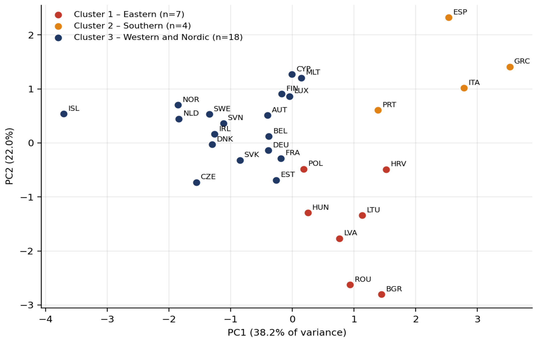
The first component, at 38.2% of the variance, opposes unemployment and inequality to labour force participation and fertility; the second, at 22.0%, is dominated by life expectancy, which is what separates the eastern from the southern group.
The three social configurations do differ in plastic packaging generation, and this is the principal result of the section. Cluster averages of generation per capita are 22.9, 32.0 and 32.7 kilograms respectively. Analysis of variance rejects equality at F(2, 26) = 4.22 with p = 0.026, and the Kruskal–Wallis test agrees, with H = 6.76 and p = 0.034.
Figure 15.
External validation and cluster profiles. Note. Left: plastic packaging generation by cluster, boxes with individual countries overlaid. Right: cluster means in standard deviations from the sample mean. Clusters differ significantly in generation, F(2,26) = 4.22, p = 0.026.
Figure 15.
External validation and cluster profiles. Note. Left: plastic packaging generation by cluster, boxes with individual countries overlaid. Right: cluster means in standard deviations from the sample mean. Clusters differ significantly in generation, F(2,26) = 4.22, p = 0.026.
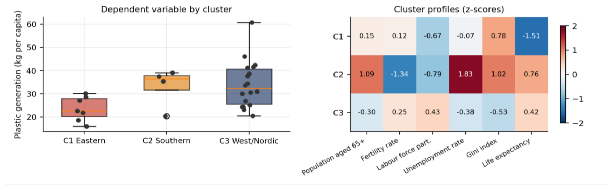
Pairwise comparison locates the difference precisely. The eastern cluster generates 0.352 log points less than the western and Nordic cluster, a gap of roughly 30% in levels, significant at t = −3.17 with p = 0.007. The southern cluster is statistically indistinguishable from the western one, at a difference of 0.022 with p = 0.903, and its difference from the eastern cluster falls just short of conventional significance at p = 0.121, reflecting a group of only four countries.
The finding is therefore a binary rather than a threefold distinction: the post-transition economies generate substantially less plastic packaging per head, while southern and north-western Europe do not differ from one another despite very different labour market and demographic profiles. High unemployment and demographic contraction, which define the southern group, do not translate into lower packaging generation once the level of development is comparable.
This contrasts sharply with the environmental clustering of Section 5, where the three environmental types were statistically indistinguishable in packaging generation. Social configuration carries information that environmental configuration does not, which is consistent with the panel results, where the social block explained 52.6% of the between-country variance against 46.5% for the environmental block.
9. Machine Learning Validation of the Social Model
The purpose of this section is validation, not forecasting. A linear panel specification that is outperformed by algorithms free to fit interactions and thresholds on the same information is misspecified; one that matches or beats them has extracted the signal available in the data. The second question is whether a non-parametric learner, left free to select, assigns importance to the same variables as the econometric model.
Six algorithms are compared: linear regression, linear support vector regression, k-nearest neighbours, a pruned decision tree, a random forest of eight hundred trees and gradient boosting with five hundred stages. All use the six social indicators of Section 7.
Validation is by ten-fold cross-validation grouped by country, so that every observation of a country lies either in the training or in the test partition and never in both. In a panel this is essential: with random folds a learner recovers a country’s level from its adjacent years and returns a fit that measures memorisation. Two exercises are run. The first predicts the level of the logarithm of plastic packaging generated per capita, corresponding to the between dimension and to the question of predicting an unseen country. The second predicts the country-demeaned series, corresponding to the fixed-effects transformation. See Table 12.
The two linear methods occupy the first two positions, with the support vector formulation ahead on four of six measures and a mean rank of 1.17. The three flexible learners return negative cross-validated R2, meaning that predicting the sample mean for every observation would be more accurate than their fitted values, with the decision tree worst at −0.470. This is the signature of overfitting to country-specific levels: in a panel of 29 countries observed ten times, the partitions a tree learns correspond to individual countries, and when a country is withheld entirely those partitions carry no information. See Figure 16.
The within-transformed exercise, unlike its environmental counterpart, does not reverse the ranking. The linear support vector regression is again first at 0.376 and linear regression second at 0.362, ahead of k-nearest neighbours at 0.332, the decision tree at 0.328, the random forest at 0.295 and boosting at 0.230. The linear form is therefore adequate in both dimensions of the social specification, which is a stronger validation than the environmental block obtained: there, flexible learners gained roughly 0.25 in R2 on the demeaned data, whereas here they lose between 0.04 and 0.15.
One qualification applies to the second exercise in both sections. The demeaning uses each country’s own average, including the years assigned to the test fold, so it is a comparison of functional forms on transformed data rather than a clean out-of-sample test. The conclusion drawn here is conservative in that respect, since it states that flexibility does not help.
The decisive validation concerns which variables matter. Table 13 reports permutation importance, computed on the held-out fold at each split and averaged over the ten splits.
The two exercises rank the variables differently, and the pattern reproduces the econometric results with unusual precision. In levels, life expectancy is by a wide margin the most important predictor, followed by the Gini index and unemployment; population ageing and fertility have importance indistinguishable from zero or negative. This is exactly the ordering of the Between and Pooled, where life expectancy carried standardised coefficients of 0.632 and 0.607, the Gini index 0.371 and 0.348, and unemployment 0.440 and 0.434, while ageing and fertility were insignificant.
In the within-transformed exercise the ordering inverts. Population ageing becomes the most important variable in both models, followed by unemployment, while life expectancy and the Gini index fall to zero. This reproduces the fixed-effects column, where ageing carried the largest standardised coefficient at 0.361 and was significant at the 5% level, unemployment followed at 0.176, and the Gini index was both the smallest and the least significant. See Figure 17.
The sign reversal on life expectancy documented in Section 7.4 therefore receives independent confirmation. A learner that knows nothing about panel econometrics finds life expectancy highly informative when comparing countries and worthless when tracking a country over time, which is precisely the diagnosis offered there: between countries the variable proxies the level of development, within a country over ten years it does not.
Three conclusions follow for the specification of Section 7.
The linear form is adequate in both dimensions. No algorithm capable of representing non-linearities improves on the linear models in either exercise, so the functional form assumption of the panel is not costing explanatory power. This is a stronger statement than a specification test because it is made out of sample.
The variable hierarchy is robust to method and dimension-specific. Two independent approaches recover the same two orderings, one for the cross-section and one for the time dimension, and both reproduce the divergence that the Mundlak test rejects at χ2(6) = 33.91. The econometric result is not an artefact of the linear estimator.
The ceiling on cross-country accuracy remains modest. A cross-validated R2 of 0.172 means that roughly five sixths of the between-country variation in plastic packaging generation is unexplained by the social block even when learners are allowed to search for structure, against 0.191 for the environmental block. In-sample explained variance of 0.526 and 0.465 respectively is therefore not a guide to out-of-sample performance, and the difference between the two figures is the amount by which conventional panel R2 overstates what these variables can actually predict.
10. Panel Analysis: The Governance Component
The dependent variable remains the natural logarithm of plastic packaging waste generated per capita. The governance block draws on the corresponding pillar of the World Bank ESG Data Framework and comprises six regressors.
The six Worldwide Governance Indicators are not entered separately. Their pairwise correlations lie between 0.895 and 0.965, so a specification containing all of them would produce unstable coefficients whose signs alternate across specifications. They are replaced by their first principal component, which accounts for 84.5% of their joint variance and loads almost uniformly across the six dimensions, with weights between 0.275 for political stability and 0.438 for rule of law. This component is interpreted as an index of institutional quality. Appendix G5 reports the six indicators entered individually as a robustness check.
The remaining regressors are the annual growth rate of GDP, which captures the cyclical position; net migration in signed logarithmic form, which measures population inflow independent of natural change; the share of individuals using the internet, which proxies the penetration of digital commerce and therefore of parcel and delivery packaging; the share of parliamentary seats held by women, a standard measure of political inclusion; and research and development expenditure as a share of GDP, a measure of innovation capacity. Variance inflation factors range from 1.10 to 3.32.
The estimation sample covers 29 countries between 2014 and 2023, for 282 observations, unbalanced between seven and ten years per country. Figure 18 decomposes the variation of each variable.
The block is heterogeneous in this respect. GDP growth is almost entirely a within phenomenon, at 0.663, and net migration and internet penetration exceed 0.38, whereas institutional quality at 0.113 and R&D expenditure at 0.151 barely clear the ten per cent threshold. This asymmetry determines what the fixed-effects estimator can identify and anticipates the results. See Table 14.
The block explains 56.6% of the between-country variance, the highest figure obtained for any of the three pillars, and 46.6% within countries. Two coefficients are robust across the within estimators. GDP growth carries 0.0041 under fixed effects, 0.0042 under random effects and 0.0042 in the dynamic specification, all significant at the 1% level: a percentage point of additional growth is associated with a rise of 0.41% in plastic packaging generated per head, which is the cyclical response of packaged consumption. Internet penetration carries 0.0127 under fixed effects and 0.0128 under random effects, both at the 1% level, and remains significant in the dynamic column at 0.0033. See Figure 19.
The result that matters most for the interpretation of the pillar is negative. Institutional quality is not significant in any of the six columns, with p-values between 0.14 and 0.79 and a coefficient that varies between 0.009 and 0.046 without stabilising. Net migration is significant between countries, at 0.0292, but not within them.
| Test | Null hypothesis | Statistic | p-value |
| F test on individual effects | No country effects (pooling) | F(28, 247) = 61.93 | 0.000 |
| Breusch–Pagan LM | No random effects | χ2(1) = 78.69 | 0.000 |
| Mundlak Wald (robust Hausman) | Within equals between | χ2(6) = 18.80 | 0.005 |
| Pesaran CD | Cross-sectional independence | CD = 0.09 | 0.927 |
| Wooldridge AR(1) | No first-order serial correlation | ρ̂ = 0.548 | 0.000 |
| Breusch–Pagan | Homoskedasticity | χ2(6) = 9.75 | 0.136 |
Pooling is rejected and the Mundlak test rejects equality of the within and between relationships, so the fixed-effects column is the one to interpret. Two results are more favourable than in the previous sections. The Pesaran statistic of 0.09 does not reject cross-sectional independence, as in the social block and unlike the environmental one, and the Breusch–Pagan test does not reject homoskedasticity, the only pillar for which this holds. Serial correlation remains, at 0.548, and is addressed by clustering.
The null result on institutional quality is examined further because it is the substantive question the pillar was meant to answer. Figure 20 reports each of the six Worldwide Governance Indicators entered individually in place of the composite index, holding the rest of the specification fixed.
None reaches significance at the 10% level. Political stability comes closest, at 0.115 with p = 0.111, and rule of law follows at 0.124 with p = 0.235; regulatory quality, the indicator with the strongest prior claim given that packaging is governed by a European directive, returns −0.011 with p = 0.885. Explained variance is essentially unchanged across the six, between 0.464 and 0.479. The composite index is therefore not concealing a result that individual indicators would reveal.
The interpretation is the one suggested by Figure 1. Institutional quality has a within share of 0.113: over ten years the governance indicators of European countries barely move, and the fixed-effects estimator has almost no information to work with. Between countries the variation is ample, but there the coefficient is also insignificant, at 0.038 with p = 0.485. The conclusion is not that institutions are irrelevant to packaging, but that aggregate governance indices do not discriminate among European economies on this outcome.
The autoregressive coefficient is 0.653, implying that about 35% of the gap from equilibrium closes each year and a long-run multiplier of 2.88. GDP growth and internet penetration remain significant in the dynamic specification, which distinguishes this pillar from the social one where no coefficient survived the introduction of the lag.
Inference was re-assessed by a wild cluster bootstrap-t with Rademacher weights and the null imposed, on 1,999 replications. Internet penetration returns a bootstrap p-value of 0.0005 and GDP growth 0.0120; the remaining four lie between 0.23 and 0.72. Internet penetration passes a Bonferroni correction over six tests, which requires 0.0083, and is the only coefficient in the three pillars other than the two environmental intensities to do so.
Appendix G3 adds log GDP per capita, which is insignificant at 0.087 with p = 0.476, leaving internet penetration at 0.0114 with p = 0.001. Appendix G6 replicates the specification on total packaging generation, where explained variance rises to 0.582 and both focal coefficients retain sign and significance.
The governance pillar explains the largest share of between-country variance of the three, but the mechanism that carries the result is not governance in the institutional sense. It is the growth cycle and the diffusion of digital commerce. Internet penetration is the strongest single coefficient in the entire study by bootstrap significance, and its interpretation is direct: a ten-point rise in the share of the population online is associated with a rise of roughly 13% in plastic packaging generated per capita, consistent with the substitution of parcel and delivery packaging for retail purchase.
The negative finding on institutional quality is worth as much as the positive ones. Across three pillars, twenty-eight countries and ten years, the composite governance index and all six of its components fail to explain how much plastic packaging European economies place on the market. If institutions matter here, they matter through instruments specific to the domain, such as extended producer responsibility schemes and deposit-return systems, rather than through general measures of state capacity.
Judged on statistical significance, this is the strongest of the three panel models. It has the highest between R2, the cleanest diagnostics, two coefficients significant across five and six of the six estimators respectively, and the single most robust coefficient of the study under bootstrap inference. Judged on publishability, its value lies as much in the null result on institutional quality, which is precise, extensively probed and cleanly reported, as in the two positive findings.
11. Cluster Analysis of the Governance Component
The panel estimates of Section 10 identify partial effects of individual governance indicators. This section asks whether European economies fall into distinct governance configurations and whether membership of a configuration carries information about the quantity of plastic packaging placed on the market. The units are the 29 countries of the estimation sample, described by the six governance indicators averaged over 2014–2023 and standardised, with all variables winsorised at the first and ninety-ninth percentiles beforehand. The dependent variable is excluded from the classification space and reserved for external validation. Six algorithms were estimated at three clusters; the following Table 15 reports eleven validity indices.
DBSCAN is excluded from the ranking on the same grounds as in the previous two sections: its indices are computed on 55% of the sample, and its Dunn index of 0.816 and maximum diameter of 2.00 are consequences of discarding the dispersed observations rather than evidence of structure.
The governance block is markedly better suited to clustering than the other two. Explained variance reaches 0.622 against 0.430 for the social block and 0.422 for the environmental one, the silhouette is 0.370 against 0.256 and 0.245, and the Calinski–Harabasz index is 21.37 against 9.82 and 9.13. Governance configurations in Europe are more sharply delineated than social or environmental ones. See Figure 21.
K-Means obtains the best mean rank at 1.91, ahead of the Gaussian mixture at 2.59, Ward at 2.86 and Fuzzy C-Means at 2.91, with random forest proximity last at 4.73. K-Means ranks first on six indices, including explained variance, both information criteria, Calinski–Harabasz and maximum diameter. Ward and the mixture attain marginally higher silhouettes, 0.379 and 0.378 against 0.370, and better separation, but produce more concentrated partitions. The margin between the first four algorithms is narrow, which is itself informative: when the underlying structure is strong, the choice of algorithm matters less. See Figure 22.
The number of clusters is less clear-cut than in the previous sections. The silhouette is highest at two clusters, at 0.387, and declines monotonically thereafter. The within sum of squares falls by 22.2 at the third cluster and by 19.6 at the fourth, so the elbow is not sharp. Calinski–Harabasz is highest at two, at 26.40. Three clusters is retained on the grounds of interpretability and group balance, and because the two-cluster partition merely separates western from eastern Europe without adding information beyond what a per-capita income split would provide. This choice is acknowledged as weaker than in Section 5 and Section 8 and is treated as such in the discussion. See Table 16.
The first cluster contains fourteen countries, from Austria and Belgium to Sweden and Norway, plus Estonia, Slovenia and Spain. It is defined by institutional quality at 0.78 standard deviations above the mean, the highest R&D expenditure, the highest share of women in parliament at 37.5%, and the lowest growth at 1.9% annually. It is the mature institutional configuration.
The second gathers eleven eastern and southern economies. Every indicator except growth lies below the mean, with institutional quality at −0.88 and internet penetration at −0.97, the latter corresponding to 76.0% of the population online against 91.0% in the first cluster.
The third contains only Cyprus, Hungary, Ireland and Malta, and is defined by growth at 1.87 standard deviations above the mean, averaging 5.5% annually, combined with the lowest representation of women in parliament at 16.2%. Its coherence rests on the growth dimension, and with four members it should be treated as a distinctive group rather than as a type. See Figure 23.
The first component accounts for 64.5% of the variance, the highest concentration of the three pillars, and loads positively on every indicator except growth: it is an institutional development axis. The second, at 18.5%, is dominated by growth and separates the third cluster from the other two. The three configurations differ in plastic packaging generation. Cluster averages are 34.2, 24.5 and 34.2 kilograms per capita, and equality is rejected by analysis of variance at F(2, 26) = 5.27 with p = 0.012 and by the Kruskal–Wallis test at H = 8.13 with p = 0.017. See Figure 24.
Pairwise comparison again locates the difference in a single contrast. The eastern and southern cluster generates 0.334 log points less than the institutionally strong cluster, a gap of roughly 28% in levels, significant at t = 3.39 with p = 0.003. The high-growth cluster is indistinguishable from the institutionally strong one, at a difference of 0.001 with p = 0.997, and its difference from the eastern cluster does not reach significance at p = 0.237, reflecting a group of four countries.
The result therefore replicates the social clustering of Section 8 almost exactly: a binary contrast between the eastern and southern periphery and the rest, with the third group aligned to the wealthier side. The two partitions are not identical — Czechia, Italy and Portugal move between them — but they identify the same divide.
This is the interpretative difficulty of the section. The governance partition separates the dependent variable, but so does the social partition, and both separate it along a boundary that coincides with the distribution of income in Europe. Cluster analysis on aggregate country indicators cannot distinguish a governance effect from a development effect, because in this sample the two are nearly collinear: the first principal component of the governance block correlates at 0.75 with internet penetration and at 0.68 with R&D expenditure, both of which are themselves markers of economic maturity.
The technical quality of this partition is the highest of the three: explained variance of 0.622, silhouette of 0.370, a first principal component absorbing 64.5% of the variance, unanimous agreement among the four leading algorithms, and analysis of variance significant at the 0.01% level on every constituent indicator. The external validation succeeds where the environmental one failed.
The substantive contribution is nonetheless more limited than those figures suggest, for two reasons stated plainly. The choice of three clusters is not supported by the internal criteria, which favour two. And the recovered contrast is the same east-west divide identified by the social clustering, which in turn tracks income, so the section cannot claim that governance configuration as such determines packaging generation.
On publishability, the assessment is that this section is a solid supporting component rather than a standalone contribution. It would not sustain a paper on its own; within a nine-module study it earns its place by documenting a well-defined partition, by validating it externally and by acknowledging that the validation does not identify a governance channel. Its most quotable finding is the negative one, consistent with Section 10.4: neither the composite institutional index in the panel nor the governance typology here isolates an institutional effect on how much plastic packaging European economies produce.
12. Machine Learning Validation of the Governance Model
The exercise is validation rather than forecasting. A linear panel specification outperformed by algorithms free to fit interactions and thresholds on the same information is misspecified; one that matches or beats them has extracted the available signal. The second question is whether a non-parametric learner assigns importance to the same variables as the econometric model.
Six algorithms are compared on the six governance regressors of Section 10: linear regression, linear support vector regression, k-nearest neighbours, a pruned decision tree, a random forest of eight hundred trees and gradient boosting with five hundred stages. Validation uses ten-fold cross-validation grouped by country, so that all observations of a country lie either in the training or in the test partition. Two exercises are run: prediction of the level of the logarithm of plastic packaging generated per capita, corresponding to the between dimension, and prediction of the country-demeaned series, corresponding to the fixed-effects transformation. See Table 17.
This is the first block in which the flexible learners win, and the margin is wide. The random forest attains a cross-validated R2 of 0.445 and boosting 0.439, against 0.130 for linear regression and 0.082 for the support vector formulation. Every non-parametric method, including the pruned decision tree, outperforms both linear models. The mean absolute percentage error falls from 7.01% to 5.70%. See Figure 24.
Figure 24.
Predictive performance of six algorithms, levels and within-transformed.
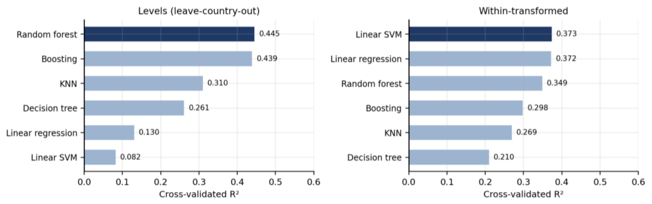
The within-transformed exercise reverses the ordering. The linear support vector regression is first at 0.374 and linear regression second at 0.372, ahead of the random forest at 0.349, boosting at 0.298, k-nearest neighbours at 0.269 and the decision tree at 0.210.
The two exercises therefore deliver opposite verdicts on functional form, and the conclusion is specific rather than general. Within countries the linear fixed-effects specification of Section 10 is adequate and nothing is gained from flexibility. Between countries it is not: the governance indicators relate to packaging generation in a way that a linear model captures poorly, and roughly 0.31 of cross-validated R2 is left unexploited by the linear specification. This is the first evidence of genuine misspecification in the study, and it is confined to the cross-sectional dimension of the governance pillar. See Table 18.
Institutional quality is the most important predictor in both flexible models in levels, at 0.0241 and 0.0277, and is nearly four times as important under the random forest as under linear regression, at 0.0065. This is the variable that the panel of Section 10 found insignificant in every one of the six estimators, with a between coefficient of 0.038 and p = 0.485. See Figure 25.
The reconciliation is in the shape of the relationship rather than in its strength. Figure 26 plots the partial dependence of the random forest in levels against the linear slope estimated by the between estimator.
The curve for institutional quality is not monotone. Packaging generation is flat across the lower half of the institutional range and rises only above roughly the sample median, so a straight line fitted through the whole range averages a null segment with a positive one and returns a slope indistinguishable from zero. The panel result of Section 10.4 was therefore correct as a statement about linear association and incomplete as a statement about the variable: institutional quality does not enter linearly, but it does carry cross-sectional information.
Internet penetration behaves differently. It is important in all four columns, including 0.0106 in the within-transformed model where every other variable falls to zero, and its partial dependence is close to linear. This is the coefficient that survived the wild cluster bootstrap at p = 0.0005 in Section 10, and it is the only variable in the governance block whose importance is confirmed by both dimensions and by both classes of model.
GDP growth is the mirror image. It has essentially zero importance in levels, which is expected since it is almost entirely a within phenomenon with a within share of 0.663, and its predictive contribution appears only in the panel estimates rather than in a cross-sectional exercise.
Three conclusions follow.
The linear specification is adequate within countries and inadequate between them. This qualifies the between R2 of 0.566 reported in Section 10: the linear model attains that figure in sample but generalises at 0.130, whereas a random forest generalises at 0.445. The gap between in-sample fit and out-of-sample performance is larger here than in either of the other two pillars.
The null result on institutional quality requires restatement. It holds for linear association, has been probed through the composite index and all six of its components, and is not overturned by the panel evidence. But a non-parametric learner assigns it the highest importance in the cross-section, and the partial dependence shows why: the relationship is a threshold rather than a slope. The honest formulation is that institutional quality is not linearly related to packaging generation, not that it is unrelated.
Internet penetration is confirmed as the most robust single finding of the governance pillar. It is significant in the panel, survives bootstrap and Bonferroni correction, and is the only variable that a learner ranks highly in both the level and the demeaned exercise.
13. Discussion
Table 19 summarises the nine modules. Each row reports what the panel estimator identified, whether the clustering partition separated the dependent variable, and what the supervised learners concluded about functional form and variable importance.
Three regularities emerge from the table. First, the between dimension is consistently better explained than the within dimension in sample, yet consistently worse predicted out of sample: cross-validated R2 falls to between 0.172 and 0.445 against in-sample figures of 0.465 to 0.566. Second, the two methods disagree productively rather than redundantly, and where they disagree the disagreement is informative. Third, only three coefficients across eighteen survive both the bootstrap and a correction for multiple testing, which is the honest measure of what this design establishes.
In line with expectations. The cyclical response of packaging generation to growth and unemployment confirms the decoupling literature. The elasticity of 0.0041 on GDP growth and of −0.014 to −0.036 on unemployment are consistent with Koçak and Bağlıtaş (2022) and with the partial decoupling reported by Mazzanti and Nicolli (2011) for the EU15. The persistence coefficients between 0.65 and 0.71 corroborate Chakraborty et al. (2022) on the slowness of structural change in waste-income relationships. The demographic result on ageing is consistent with Rybová et al. (2018), and the finding that the social pillar outperforms the environmental one in the cross-section aligns with Hondroyiannis et al. (2024a).
In contradiction with expectations. Institutional quality does not enter linearly, in any specification, through the composite index or through any of its six components. Given Chalak et al. (2016), who find legislation and regulation significant in a 44-country analysis, and given the packaging literature’s premise that producer responsibility design shapes outcomes (Joltreau, 2022; Colelli et al., 2022), a positive association was expected and is absent. The environmental clustering delivers a second contradiction: three sharply separated environmental types are statistically indistinguishable in packaging generation, which no reading of the material flow literature would have predicted.
New. Internet penetration emerges as the most robust determinant in the study, at roughly 13% additional plastic packaging per ten percentage points of population online. The e-commerce strand had described the mechanism qualitatively (Khatami et al., 2023; Tyagi et al., 2021) but had not estimated it on a generation outcome. The second novelty is methodological: the threshold shape of the institutional relationship, invisible to six linear estimators and recovered by partial dependence, reconciles the null result with the policy literature and suggests that institutional quality matters only above a capacity floor.
Two implications follow for policy. Targeting on environmental profile is unlikely to be productive, since environmental types carry no information about packaging burden; targeting on the two specific intensities identified by the panel does carry information. And because the diffusion of online retail is the strongest single correlate of packaging generation, instruments aimed at delivery and parcel packaging address the margin along which the burden is currently growing, whereas instruments calibrated on retail packaging address a shrinking one.
Three limits qualify these readings. The design identifies structural associations rather than causal effects: no regressor is plausibly exogenous to the material intensity of an economy, and no instrument or quasi-experimental variation is available. The panel is short and narrow, twenty-nine countries over ten years, which is why the dynamic estimator is reported as a lower bound on persistence and why the Anderson–Hsiao alternative cannot separate high persistence from a unit root. And the specification contains no time effects, so shocks common to all countries are not absorbed and coefficients on trending regressors remain the most fragile of those reported.
14. Policy Implications
The European packaging framework has been built around treatment. Recycling targets, producer responsibility schemes and deposit-return systems all operate downstream of the point at which packaging is placed on the market, and the prevention obligation that accompanies them has never acquired an equivalent apparatus of measurable objectives. The results reported here indicate why that asymmetry matters. Plastic packaging generation per capita is explained to a substantial degree by the structural characteristics of an economy, and those characteristics respond to instruments that lie outside waste policy altogether. A ministry that holds only treatment levers is working on the wrong margin if the objective is to reduce the quantity of material entering the system.
The most direct implication concerns the diffusion of online retail. The association between internet penetration and packaging generation is the most robust in this study, surviving both bootstrap inference and correction for multiple testing, and its magnitude is economically material: a ten-point rise in the share of the population online corresponds to roughly a thirteen per cent increase in plastic packaging generated per head. This is a growing margin, not a stable one, and existing instruments are poorly aligned with it. Producer responsibility fees are calibrated on packaging placed on the domestic market by producers, whereas parcel and delivery packaging is generated by logistics operators and platforms, often across borders, and frequently escapes the fee base entirely. Extending the scope of producer responsibility to transport and delivery packaging, and differentiating fees by reusability rather than by weight alone, addresses the margin along which the burden is currently expanding. The recent shift of European packaging law towards a regulation rather than a directive, which removes national transposition discretion, creates the legal vehicle for such an extension; the evidence here suggests it should be used.
The finding that composite governance quality does not predict packaging generation, in any linear specification and for any of its six components, would ordinarily counsel against institutional interventions. The machine learning module qualifies that reading in a way that carries a specific policy meaning. The relationship is a threshold: below roughly the median of the institutional distribution, variation in governance quality is unrelated to packaging outcomes, while above it the association becomes positive. Institutional capacity therefore appears to function as a precondition rather than as a continuous lever. Marginal improvements in regulatory quality or government effectiveness in countries already above the threshold are unlikely to change packaging burdens; below it, general institutional strengthening is a prerequisite for any domain-specific instrument to bind at all.
The practical corollary is that packaging policy should be designed with domain-specific instruments rather than with expectations about state capacity in general. Deposit-return systems, reusability mandates, fee modulation and reporting obligations act directly on the flows they govern. Aggregate governance indices, which are widely used as controls in this literature, do not identify the channel through which institutions matter for packaging and should not be treated as though they did.
Two results bear on how policy effort might be allocated across member states. Environmental typologies are not informative: countries that resemble one another in emissions, energy and land use do not resemble one another in packaging burden, so classifying member states by environmental profile for the purpose of differentiated targets would misallocate effort. Social and governance typologies are informative, but the contrast they recover is binary and tracks the level of development, separating the post-transition economies from the rest while leaving southern and north-western Europe indistinguishable.
This has an uncomfortable implication for the design of differentiated targets. The post-transition economies generate substantially less plastic packaging per head, and convergence in income will tend to raise their generation towards the European average unless prevention instruments are in place before that convergence occurs. Prevention policy in those countries is therefore best framed as pre-emptive rather than corrective, which is the opposite of the sequencing that treatment-focused targets currently imply. A second corollary concerns monitoring. Because the informative country groupings are social and institutional rather than environmental, the indicator sets used to benchmark member state progress on prevention would be more discriminating if they incorporated labour market and demographic variables alongside the environmental and circularity metrics that currently dominate the European monitoring framework.
15. Limitations
The design establishes structural associations, not causal effects, and the distinction is not a formality. None of the eighteen regressors can be treated as exogenous to the material intensity of an economy: energy intensity, carbon intensity, internet penetration and institutional quality are all jointly determined with consumption patterns by processes this study does not model. No instrument with a credible exclusion restriction was available, and no quasi-experimental variation exists in the window, since the major regulatory change of the period affected all member states simultaneously. The coefficients should therefore be read as conditional correlations that are robust to a demanding battery of inferential checks, not as policy multipliers.
A related limitation concerns omitted variables. The specification contains no time effects, so shocks common to all countries — energy price movements, the pandemic contraction, exchange rate cycles — are not absorbed. Coefficients on regressors that trend over the window are correspondingly the most fragile of those reported, and the reader is cautioned against reading trend co-movement as association. The choice was deliberate, on the grounds that the effects of structural change in this domain accumulate over horizons longer than the observation window and that a common time component would absorb part of the very variation the study seeks to explain, but it is a choice that a different analyst might reasonably reverse.
The panel comprises twenty-nine countries observed over at most ten years, which constrains what can be estimated. The dynamic specification is reported as a lower bound on persistence because the least squares dummy variable estimator is biased downward in short panels; the Anderson–Hsiao alternative returns autoregressive coefficients whose confidence intervals include unity and therefore cannot distinguish high persistence from a unit root. System generalised method of moments was not attempted, since the instrument count would exceed the number of cross-sectional units. With twenty-nine clusters, cluster-robust inference sits near the limit of its asymptotic justification, which is why every focal coefficient was re-assessed by wild cluster bootstrap; the reader should note that this correction reduced the number of surviving coefficients substantially, and that only three of eighteen pass a correction for multiple testing.
The Eurostat series begins in 2014 because earlier observations were discontinued when reporting methodology was revised. This truncation removes the pre-crisis period, during which the waste–income relationship in Europe behaved differently, and it prevents any assessment of whether the associations reported here are stable across regimes. The series also carries breaks flagged by the reporting authority in a substantial number of country-years; these were not treated, and a specification that excluded them would rest on an appreciably smaller sample.
The estimation windows differ across pillars, from 2014–2022 for the environmental block to 2014–2023 for the other two, and the country composition differs by one unit. A common-sample restriction was rejected because it would have cost roughly fifteen per cent of observations, and the coefficient signs are unaffected, but strict comparability across the three pillars is correspondingly weakened.
The clustering module rests on country means and therefore discards the temporal dimension entirely. With twenty-nine units in six dimensions, density-based classification could not be applied on comparable terms and was excluded from the algorithm ranking, and the choice of three clusters in the governance block was made on interpretability rather than on internal criteria, which favoured two. The machine learning module’s within-transformed exercise uses each country’s own mean, including test-fold years, so it compares functional forms rather than testing out of sample; the conclusions drawn from it are conservative for that reason but not clean.
Finally, the ESG partition is inherited from the World Bank framework rather than derived from theory. It has the merit of being external to the analysis and therefore not selected to produce results, but several indicators could defensibly sit in a different pillar, and the governance block in particular is carried by variables that are not institutional in character. The dependent variable itself carries a further caveat: reported generation depends on national measurement conventions as much as on physical flows, and the accounting inconsistencies documented in the material flow literature imply a measurement error component that no estimator applied here can separate from genuine cross-country variation.
16. Conclusions
This study asked what determines the quantity of plastic packaging waste that European economies place on the market, and organised the answer around the three pillars of the sovereign ESG framework, each analysed through panel estimation, unsupervised classification and supervised learning.
The environmental pillar operates through the metabolic intensity of production rather than through natural endowment. Energy intensity and carbon intensity per capita are robustly associated with packaging generation and survive every inferential check imposed, including correction for multiple testing, while land-based indicators cannot be identified because they scarcely vary within countries over the observation window. The pillar nonetheless fails its typological test: environmental country types, cleanly separated on every indicator used to construct them, carry no information about packaging burden.
The social pillar explains cross-country differences better than the environmental one and passes the typological test, though the contrast it recovers is binary and coincides with the post-transition boundary. Its most defensible result is the cyclical response of packaging generation to unemployment, which holds its sign in both dimensions of the panel. Its most instructive is the sign reversal on life expectancy, which the machine learning module confirms independently by recovering opposite variable hierarchies in the cross-sectional and time dimensions.
The governance pillar produces the single most robust association in the study, between the diffusion of online retail and packaging generation, and the single most consequential null result, on composite institutional quality. The two are connected: the pillar performs well through channels that are not institutional, while the institutional channel itself is invisible to linear estimation and appears, under unrestricted functional form, as a threshold rather than a gradient. That reconciliation between an econometric null and a machine learning positive is the principal methodological contribution, and it was available only because the third module was designed to validate the specification rather than to forecast.
Three broader conclusions follow. Cross-country panels of this size support association but not causation, and the honest reporting of how few coefficients survive demanding inference is part of the result rather than a caveat appended to it. Multi-method designs earn their cost when the methods are permitted to disagree, since the disagreements in this study were more informative than the agreements. And prevention policy for packaging, unlike treatment policy, must engage with determinants that lie outside waste management, of which the growth of online retail is currently the most important.
Future work should pursue three directions: extending the analysis to the treatment side, where the institutional channel is more likely to bind; exploiting the material dimension of the Eurostat collection to test whether determinants differ across packaging fractions; and replacing aggregate governance indices with domain-specific instrument variables, which the global waste datasets now make available for a wider set of countries. Each of the three would address a limitation identified above rather than extend the present design to new territory, which is the sequencing the evidence assembled here recommends.
Appendix A
Table A1 reports the moments of the dependent variable, in both logarithmic and original units, and of the six regressors, together with the decomposition of total variation into between-country and within-country components.
Table A1.
Descriptive statistics and variance decomposition, environmental block.
| Variable | Mean | SD | Min | Median | Max | SD between | SD within | Within share |
|---|---|---|---|---|---|---|---|---|
| Plastic generation, log | 3.396 | 0.327 | 2.459 | 3.422 | 4.290 | 0.311 | 0.118 | 0.274 |
| Plastic generation, kg/capita | 31.438 | 10.303 | 11.690 | 30.640 | 72.950 | 9.840 | 3.529 | 0.264 |
| Population density (log) | 4.607 | 0.995 | 2.644 | 4.666 | 7.414 | 0.994 | 0.023 | 0.023 |
| Energy intensity | 3.230 | 0.981 | 0.970 | 3.160 | 5.980 | 0.954 | 0.267 | 0.219 |
| CO2 per capita | 6.909 | 2.896 | 3.004 | 6.366 | 17.889 | 2.771 | 0.857 | 0.236 |
| Net energy imports | 45.278 | 152.627 | −746.719 | 57.358 | 450.182 | 151.886 | 15.491 | 0.093 |
| Forest area | 35.161 | 16.750 | 1.094 | 34.454 | 73.736 | 16.883 | 0.212 | 0.012 |
| Protected areas | 21.996 | 11.837 | 0.500 | 20.200 | 55.800 | 11.754 | 2.965 | 0.201 |
Figure A1.
Country trajectories of plastic packaging generation, 2014–2022.
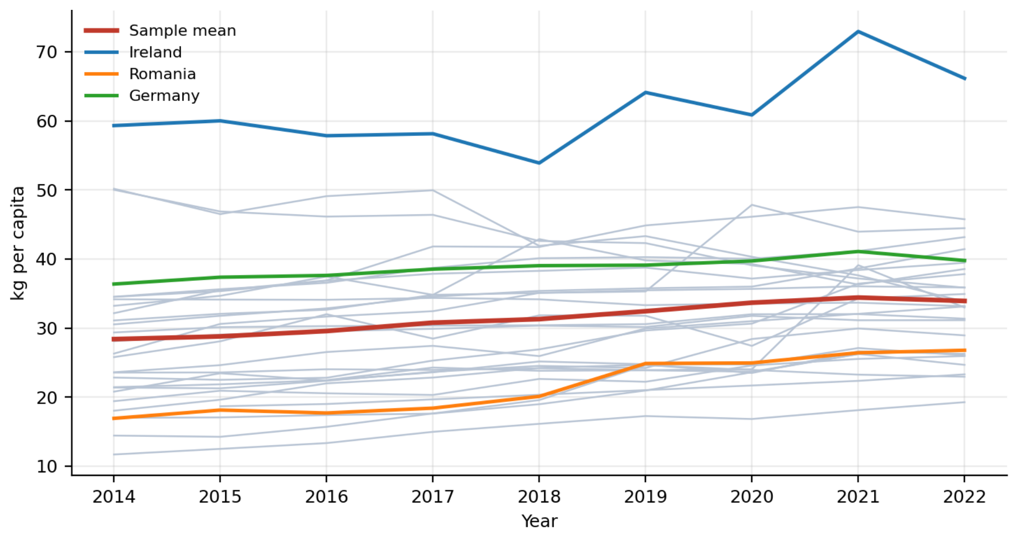
Table A2 reports pairwise correlations of the environmental block with variance inflation factors in the final column.
Table A2.
Correlation matrix and variance inflation factors, environmental block.
| Variable | Density | Energy int. | CO2 pc | Energy imp. | Forest | Protected | VIF |
|---|---|---|---|---|---|---|---|
| Population density (log) | 1.000 | −0.480 | 0.004 | 0.613 | −0.691 | 0.176 | 4.99 |
| Energy intensity | −0.480 | 1.000 | 0.314 | −0.271 | 0.606 | 0.215 | 1.81 |
| CO2 per capita | 0.004 | 0.314 | 1.000 | −0.193 | 0.102 | 0.303 | 1.30 |
| Net energy imports | 0.613 | −0.271 | −0.193 | 1.000 | −0.200 | 0.093 | 2.22 |
| Forest area | −0.691 | 0.606 | 0.102 | −0.200 | 1.000 | 0.239 | 3.71 |
| Protected areas | 0.176 | 0.215 | 0.303 | 0.093 | 0.239 | 1.000 | 1.57 |
No correlation reaches 0.70 in absolute value and no inflation factor reaches 5. Figure A2 presents the matrix graphically.
Figure A2.
Correlation matrix of the environmental block.
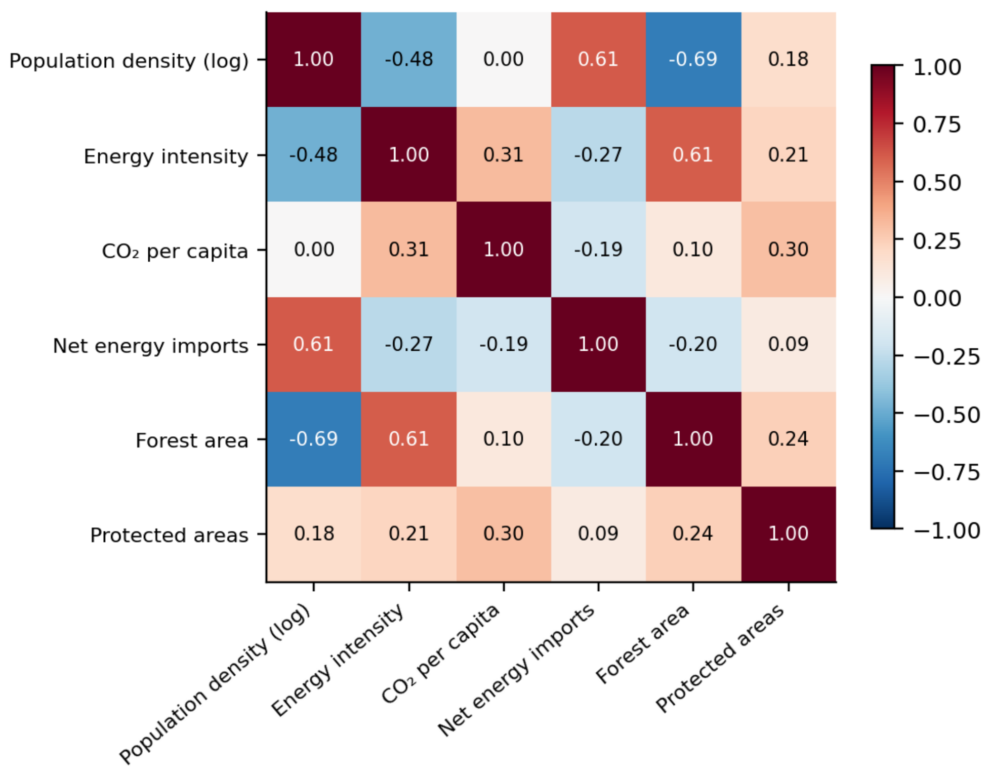
Each regressor enters together with its country mean. The coefficient on the deviation reproduces the fixed-effects estimate; the coefficient on the mean measures the gap between the between and within relationships.
| Variable | Within coefficient | Country mean |
| Population density (log) | −0.8994 | 0.9117 |
| Energy intensity | −0.4143*** | 0.2229** |
| CO2 per capita | 0.0891*** | −0.0253 |
| Net energy imports | 0.0007*** | −0.0011*** |
| Forest area | −0.0564 | 0.0586 |
| Protected areas | 0.0063** | −0.0117** |
| Note. Joint Wald test on the country means: χ2(6) = 21.25, p = 0.0017. N = 243. | ||
The mean term on carbon intensity is small and insignificant, which is the formal counterpart of the agreement between the fixed-effects and between columns of Table 1 on that variable. For density and forest area the mean terms almost exactly offset the within terms, the arithmetic signature of variables with negligible within variation.
Given a Pesaran CD statistic of 17.86, Table A4 re-estimates the model with standard errors robust to cross-sectional dependence in addition to heteroskedasticity and autocorrelation.
Table A4.
Fixed-effects estimates with Driscoll–Kraay standard errors, environmental block.
| Variable | Coefficient | DK standard error | p-value |
|---|---|---|---|
| Population density (log) | −0.8994 | 0.2726 | 0.001 |
| Energy intensity | −0.4143 | 0.0603 | 0.000 |
| CO2 per capita | 0.0891 | 0.0206 | 0.000 |
| Net energy imports | 0.0007 | 0.0006 | 0.223 |
| Forest area | −0.0564 | 0.0323 | 0.082 |
| Protected areas | 0.0063 | 0.0020 | 0.002 |
| Constant | 10.0718 | 1.4548 | 0.000 |
Point estimates are identical by construction; only the inference changes. These standard errors should be read with caution, since the Driscoll–Kraay estimator is consistent as the time dimension grows and nine periods is short; they are reported as a complement to the clustered and bootstrap results rather than as a replacement.
Table A5 adds log GDP per capita to the fixed-effects specification, to test whether the environmental associations are proxies for the level of development.
Table A5.
Fixed effects controlling for income, environmental block.
| Variable | Coefficient | Standard error | p-value |
|---|---|---|---|
| Population density (log) | −0.9155 | 0.4776 | 0.057 |
| Energy intensity | −0.2890 | 0.0709 | 0.000 |
| CO2 per capita | 0.0720 | 0.0096 | 0.000 |
| Net energy imports | 0.0007 | 0.0003 | 0.006 |
| Forest area | −0.0720 | 0.0498 | 0.150 |
| Protected areas | 0.0053 | 0.0025 | 0.036 |
| GDP per capita (log) | 0.3160 | 0.0757 | 0.000 |
Note. Fixed effects, N = 243, R2 = 0.505, clustered standard errors.
Income is itself a significant determinant, with an elasticity of 0.316. The two focal coefficients decline in magnitude by roughly 30% and 19% but retain significance at the 1% level, so they capture material and energy intensity rather than affluence.
Table A6 instruments the lagged difference of the dependent variable with its twice-lagged level in the first-differenced equation.
Table A6.
Anderson–Hsiao instrumental variables estimates, environmental block.
| Variable | Coefficient | Standard error | p-value |
|---|---|---|---|
| Lagged difference of generation | 0.9719 | 0.2461 | 0.000 |
| Δ Population density (log) | −0.4775 | 0.7187 | 0.506 |
| Δ Energy intensity | 0.0617 | 0.0551 | 0.263 |
| Δ CO2 per capita | −0.0208 | 0.0189 | 0.273 |
| Δ Net energy imports | −0.0010 | 0.0008 | 0.233 |
| Δ Forest area | −0.0038 | 0.0426 | 0.929 |
| Δ Protected areas | 0.0028 | 0.0025 | 0.270 |
Note. N = 187. First-stage F statistic on the excluded instrument: 11.53.
The autoregressive coefficient of 0.972 is close to unity and its confidence interval includes it, so the estimator cannot distinguish a highly persistent process from a unit root over nine periods. No other coefficient is significant. The estimates are reported for completeness and not used for inference; the corrected least squares dummy variable estimator of Table 1 is preferred.
Table A7 re-estimates the fixed-effects specification with the logarithm of total packaging waste generated per capita as dependent variable, over the identical sample.
Table A7.
Robustness: total packaging generation as dependent variable, environmental block.
| Variable | Coefficient | Standard error | p-value |
|---|---|---|---|
| Population density (log) | −0.9938 | 0.5574 | 0.076 |
| Energy intensity | −0.3588 | 0.0607 | 0.000 |
| CO2 per capita | 0.0648 | 0.0116 | 0.000 |
| Net energy imports | 0.0010 | 0.0004 | 0.017 |
| Forest area | −0.0578 | 0.0415 | 0.165 |
| Protected areas | 0.0035 | 0.0028 | 0.214 |
Note. Fixed effects, N = 243, R2 = 0.459, clustered standard errors.
Both focal coefficients retain sign, magnitude and significance when the dependent variable is broadened to all packaging materials, with elasticities of −0.359 and 0.065 against −0.414 and 0.089 for plastic alone. The relationship is therefore a property of packaging material throughput in general and not specific to the plastic fraction.
With 28 clusters, cluster-robust standard errors tend to over-reject. Table A8 reports bootstrap-t p-values from 1,999 replications with Rademacher weights and the null hypothesis imposed, alongside the asymptotic p-values of the fixed-effects column.
Table A8.
Wild cluster bootstrap inference, environmental block.
| Variable | Coefficient | t statistic | p, clustered | p, bootstrap |
|---|---|---|---|---|
| Energy intensity | −0.4143 | −5.89 | 0.000 | 0.0005 |
| CO2 per capita | 0.0891 | 7.50 | 0.000 | 0.0005 |
| Protected areas | 0.0063 | 2.02 | 0.030 | 0.0625 |
| Population density (log) | −0.8994 | −1.51 | 0.105 | 0.0900 |
| Net energy imports | 0.0007 | 2.52 | 0.007 | 0.1265 |
| Forest area | −0.0564 | −1.05 | 0.258 | 0.6420 |
The two focal coefficients remain significant at the 0.1% level and pass a Bonferroni correction over six tests, which requires a threshold of 0.0083.
Figure A3 plots the fixed-effects residuals against fitted values and against the time index, with the normal quantile plot.
Figure A3.
Fixed-effects residual diagnostics.
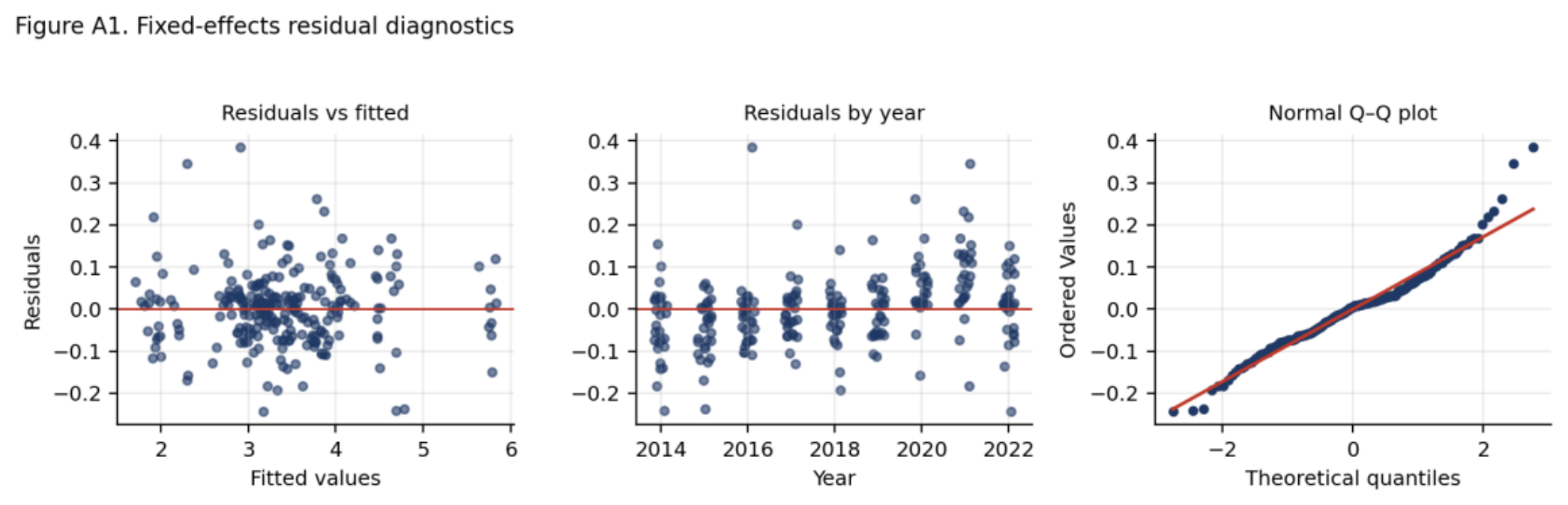
The residuals display no systematic relation to the fitted values and no drift across years. The quantile plot shows mild departure from normality in the tails, which is immaterial given the clustered and bootstrap inference reported above.
Appendix B
Table B1.
Cluster membership and silhouette widths, environmental block.
| Cluster | Countries | n | Mean silhouette |
|---|---|---|---|
| 1. Nordic-Baltic forested | Estonia, Finland, Latvia, Norway, Sweden | 5 | 0.028 |
| 2. Continental carbon-intensive | Austria, Belgium, Bulgaria, Czechia, Germany, Luxembourg, Netherlands, Poland, Slovak Republic, Slovenia | 10 | 0.206 |
| 3. Mediterranean import-dependent | Croatia, Cyprus, Denmark, France, Greece, Hungary, Ireland, Italy, Lithuania, Malta, Portugal, Romania, Spain | 13 | 0.357 |
Figure B1.
Dendrogram, Ward linkage on standardised environmental indicators.
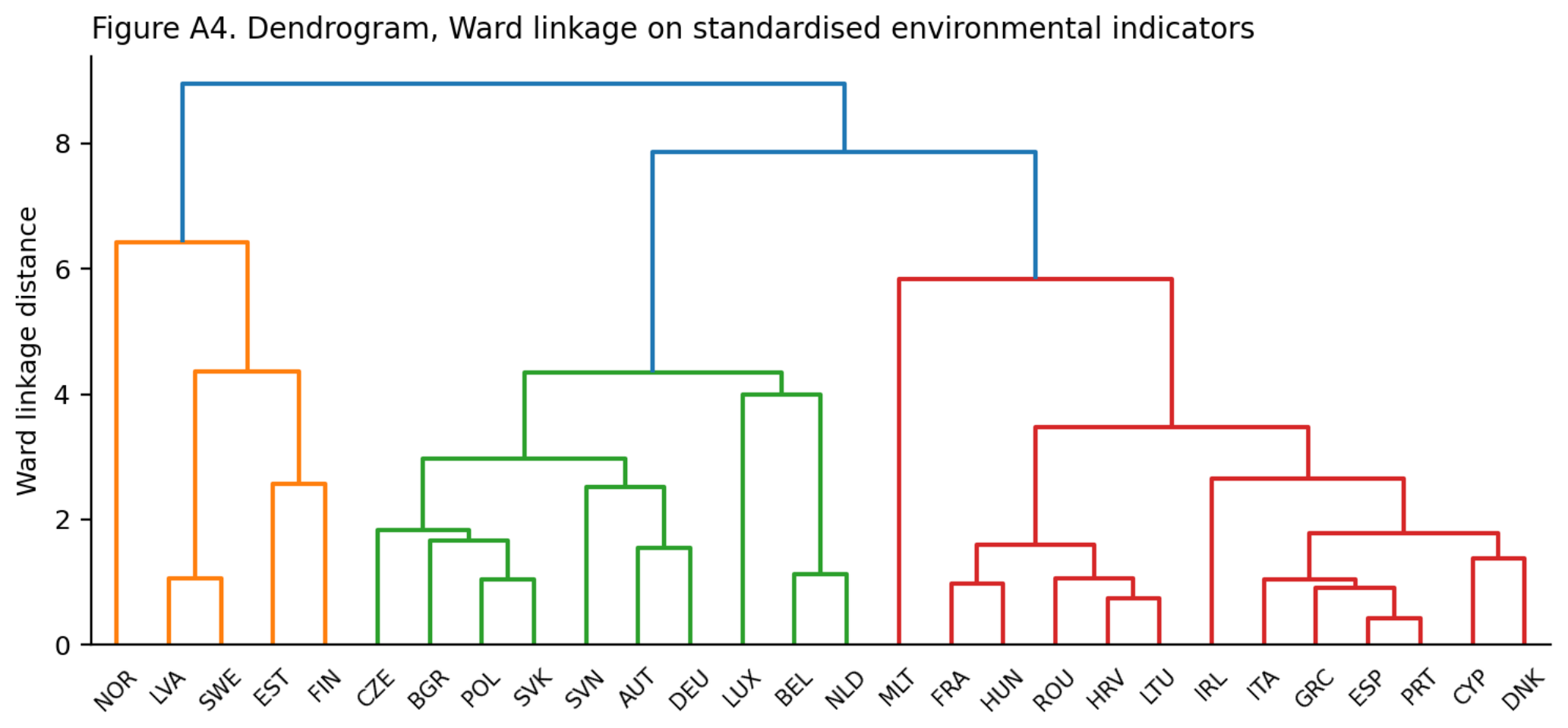
Table B2.
Selection of the number of clusters: full criteria, environmental block.
| k | R2 | Silhouette | Calinski–Harabasz | Davies–Bouldin | AIC | BIC | WSS | ΔWSS |
|---|---|---|---|---|---|---|---|---|
| 2 | 0.238 | 0.332 | 8.124 | 1.375 | 459.08 | 477.73 | 128.00 | — |
| 3 | 0.422 | 0.245 | 9.128 | 1.271 | 426.66 | 454.63 | 97.10 | 30.91 |
| 4 | 0.545 | 0.262 | 9.566 | 0.993 | 400.63 | 437.93 | 76.51 | 20.59 |
| 5 | 0.646 | 0.268 | 10.497 | 0.832 | 372.26 | 418.89 | 59.46 | 17.05 |
| 6 | 0.703 | 0.271 | 10.392 | 0.741 | 357.07 | 413.02 | 49.97 | 9.48 |
| 7 | 0.759 | 0.272 | 10.996 | 0.820 | 336.02 | 401.30 | 40.56 | 9.41 |
| 8 | 0.806 | 0.271 | 11.871 | 0.638 | 313.26 | 387.86 | 32.59 | 7.97 |
Table B3.
Cluster profiles in original units, environmental block.
| Cluster | Density (per km2) | Energy intensity (MJ/$) | CO2 (t/capita) | Net energy imports (%) | Forest (% land) | Protected (% territory) |
|---|---|---|---|---|---|---|
| 1. Nordic-Baltic forested | 22.9 | 4.109 | 7.678 | −99.6 | 57.4 | 14.5 |
| 2. Continental carbon-intensive | 164.0 | 3.566 | 8.737 | 62.2 | 35.1 | 33.1 |
| 3. Mediterranean import-dependent | 122.3 | 2.628 | 5.153 | 92.2 | 25.9 | 15.9 |
Figure B2.
Cluster profiles in standardised units.
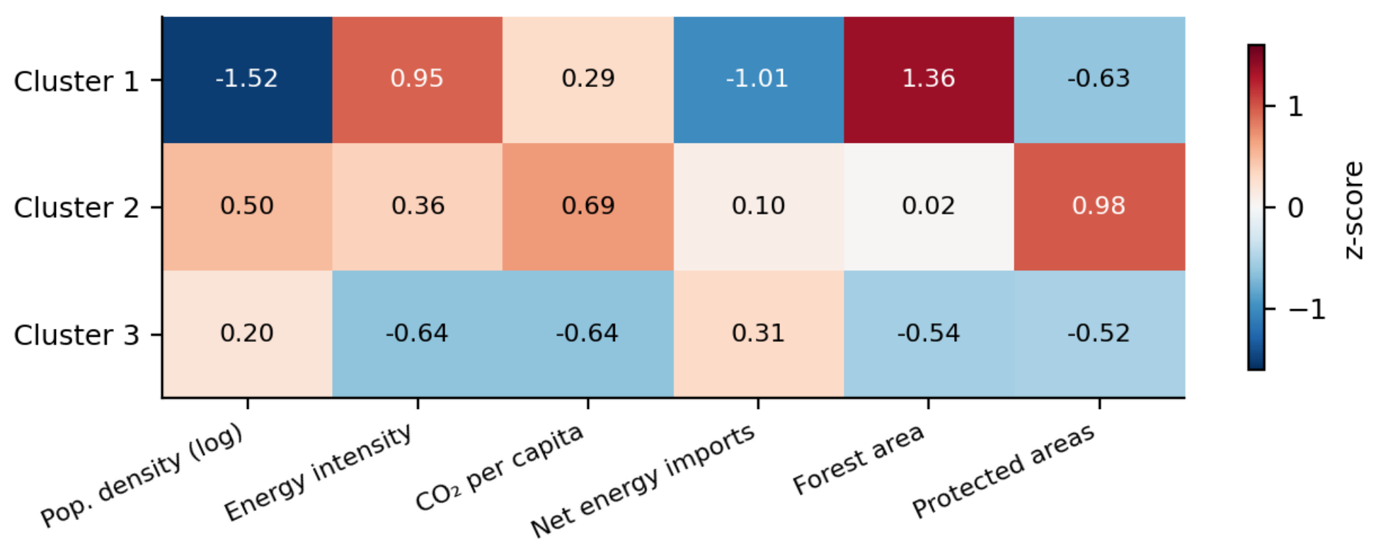
Figure B3.
Cluster quality and external validation.
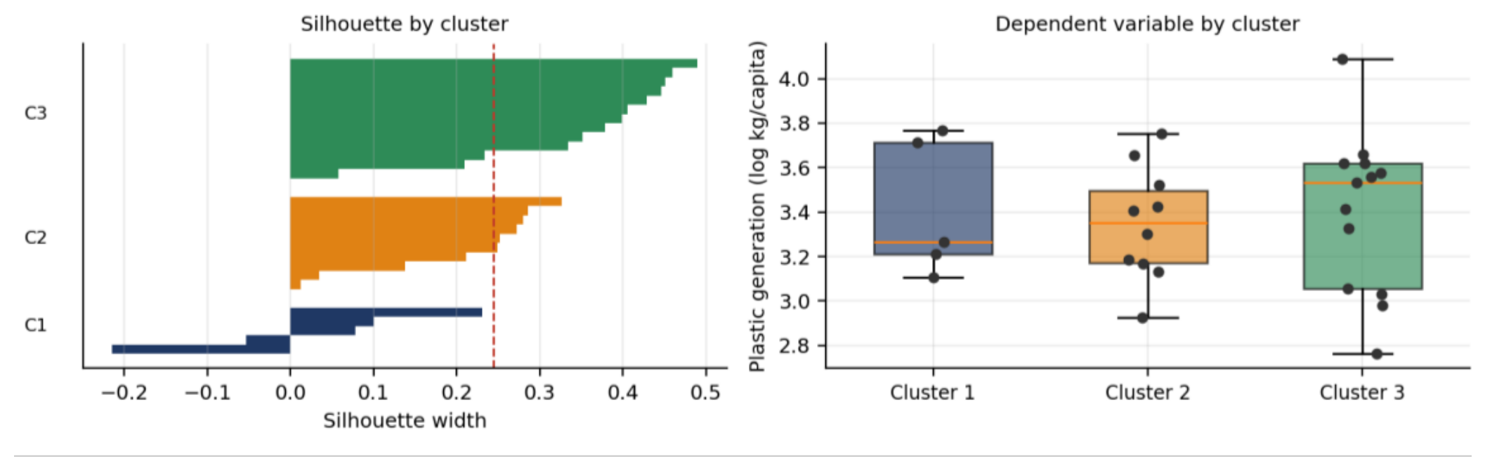
Table B4.
Analysis of variance by indicator, environmental block.
| Variable | F(2, 25) | p-value |
|---|---|---|
| Protected areas | 14.746 | 0.000 |
| Population density (log) | 13.539 | 0.000 |
| Forest area | 10.942 | 0.000 |
| Energy intensity | 8.353 | 0.002 |
| CO2 per capita | 7.465 | 0.003 |
| Net energy imports | 3.730 | 0.038 |
| Plastic generation (log), withheld | 0.108 | 0.898 |
Table B5.
Principal component loadings, environmental block.
| Variable | PC1 (42.9%) | PC2 (24.5%) |
|---|---|---|
| Population density (log) | 0.520 | 0.387 |
| Energy intensity | −0.501 | 0.168 |
| CO2 per capita | −0.206 | 0.517 |
| Net energy imports | 0.385 | 0.277 |
| Forest area | −0.518 | 0.038 |
| Protected areas | −0.141 | 0.690 |
Appendix C
Table C1.
Algorithm configurations and estimation protocol, machine learning modules.
| Algorithm | Configuration |
|---|---|
| Linear regression | Ordinary least squares on standardised predictors |
| Linear SVM | ε-insensitive regression, C = 1.0, ε = 0.05, 50,000 iterations |
| K-nearest neighbours | k = 5, distance weighting, standardised predictors |
| Decision tree | Maximum depth 4, minimum leaf size 5 |
| Random forest | 800 trees, minimum leaf size 2, all predictors considered at each split |
| Boosting | Gradient boosting, 500 stages, learning rate 0.03, maximum depth 3, subsample 0.8 |
Table C2.
Predictive performance on within-transformed data, environmental block.
| Algorithm | R2 | RMSE | MAE | Correlation | Median AE | Mean rank |
|---|---|---|---|---|---|---|
| K-nearest neighbours | 0.398 | 0.091 | 0.067 | 0.639 | 0.046 | 1.2 |
| Random forest | 0.345 | 0.095 | 0.068 | 0.619 | 0.046 | 1.8 |
| Boosting | 0.299 | 0.098 | 0.071 | 0.594 | 0.052 | 3.4 |
| Linear SVM | 0.138 | 0.109 | 0.073 | 0.478 | 0.051 | 4.4 |
| Decision tree | 0.299 | 0.098 | 0.074 | 0.596 | 0.060 | 4.4 |
| Linear regression | 0.111 | 0.111 | 0.076 | 0.445 | 0.055 | 5.8 |
Table C3.
Standardised coefficients and permutation importance compared, environmental block.
| Variable | FE standardised |β| | Pooled standardised |β| | Permutation importance (linear) |
|---|---|---|---|
| Forest area | 2.890 | 0.072 | −0.007 |
| Population density (log) | 2.739 | 0.036 | −0.004 |
| Energy intensity | 1.245 | 0.624 | 1.000 |
| CO2 per capita | 0.791 | 0.557 | 0.334 |
| Net energy imports | 0.335 | 0.136 | 0.158 |
| Protected areas | 0.229 | 0.174 | 0.091 |
Figure C1.
Partial dependence, random forest on within-transformed data.
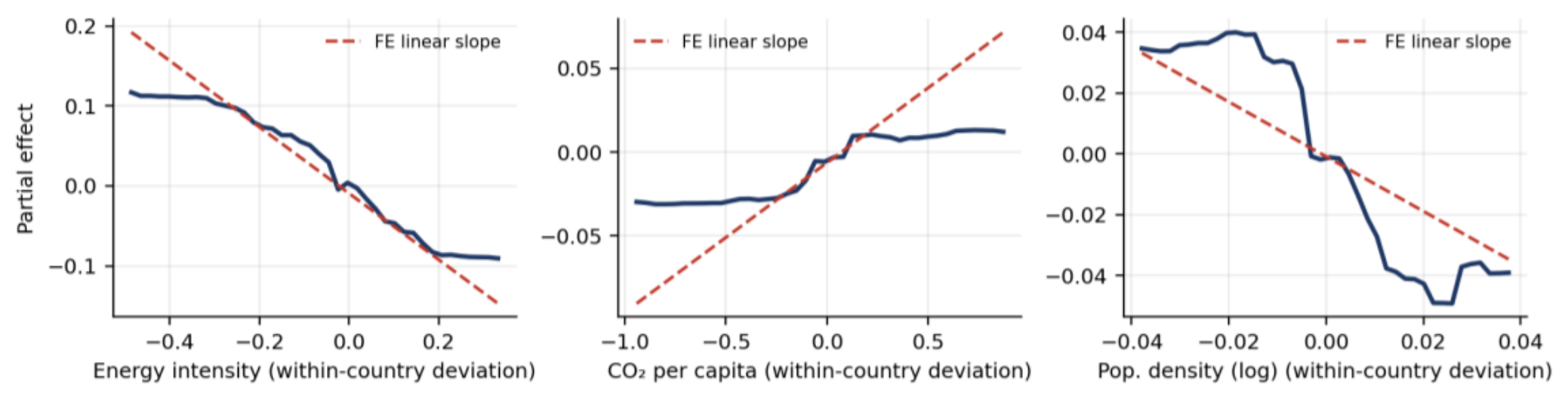
Figure C2.
Observed versus cross-validated predictions.
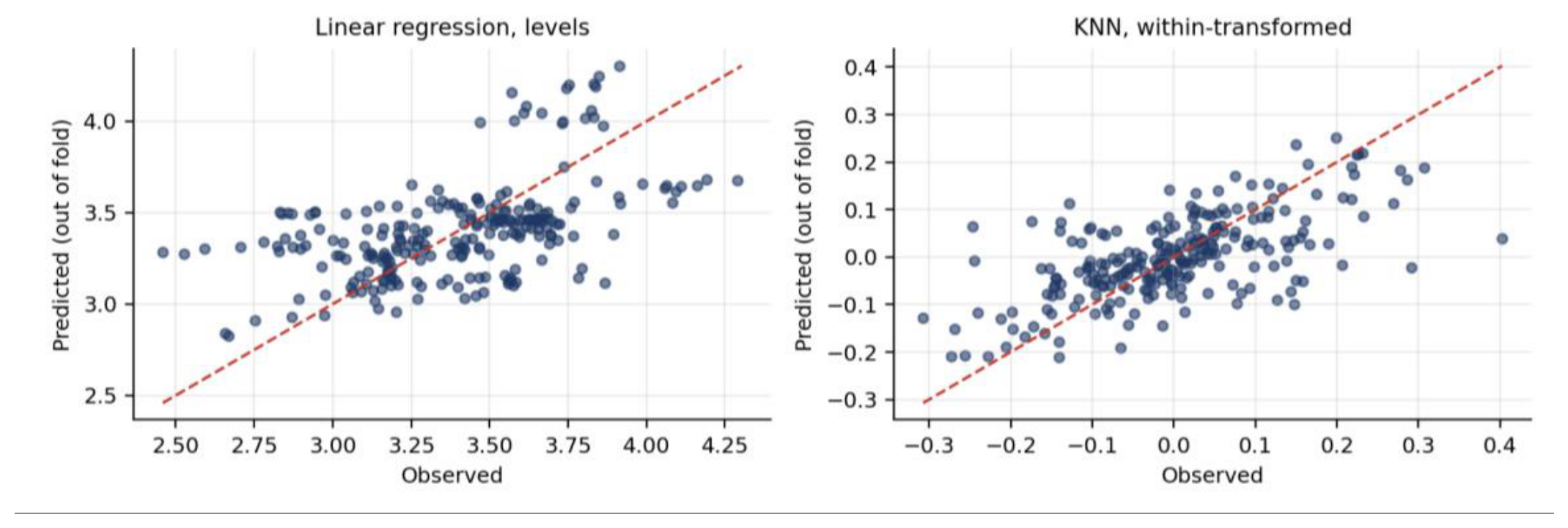
Appendix D
Table D1.
Descriptive statistics and variance decomposition, social block.
| Variable | Mean | SD | Min | Median | Max | SD between | SD within | Within share |
|---|---|---|---|---|---|---|---|---|
| Plastic generation, log | 3.400 | 0.327 | 2.459 | 3.423 | 4.290 | 0.310 | 0.116 | 0.272 |
| Population aged 65+ (%) | 18.942 | 2.645 | 12.261 | 19.411 | 24.219 | 2.556 | 0.861 | 0.252 |
| Fertility rate | 1.526 | 0.186 | 1.060 | 1.530 | 2.000 | 0.164 | 0.090 | 0.355 |
| Labour force participation (%) | 74.366 | 5.393 | 58.815 | 74.691 | 89.202 | 5.432 | 1.593 | 0.227 |
| Unemployment rate (%) | 7.414 | 4.030 | 2.015 | 6.521 | 26.708 | 3.527 | 2.059 | 0.369 |
| Gini index | 30.954 | 3.771 | 23.200 | 30.900 | 41.300 | 3.679 | 1.022 | 0.217 |
| Life expectancy (years) | 80.151 | 2.860 | 71.212 | 81.368 | 83.934 | 2.904 | 0.534 | 0.155 |
Table D2.
Correlation matrix and variance inflation factors, social block.
| Variable | Age 65+ | Fertility | LFP | Unemp. | Gini | Life exp. | VIF |
|---|---|---|---|---|---|---|---|
| Population aged 65+ | 1.000 | −0.120 | −0.103 | 0.097 | 0.202 | −0.068 | 1.05 |
| Fertility rate | −0.120 | 1.000 | 0.150 | −0.298 | −0.226 | −0.201 | 1.20 |
| Labour force participation | −0.103 | 0.150 | 1.000 | −0.377 | −0.322 | 0.249 | 1.32 |
| Unemployment rate | 0.097 | −0.298 | −0.377 | 1.000 | 0.389 | 0.094 | 1.44 |
| Gini index | 0.202 | −0.226 | −0.322 | 0.389 | 1.000 | −0.277 | 1.43 |
| Life expectancy | −0.068 | −0.201 | 0.249 | 0.094 | −0.277 | 1.000 | 1.31 |
Figure D1.
Correlation matrix, social block.
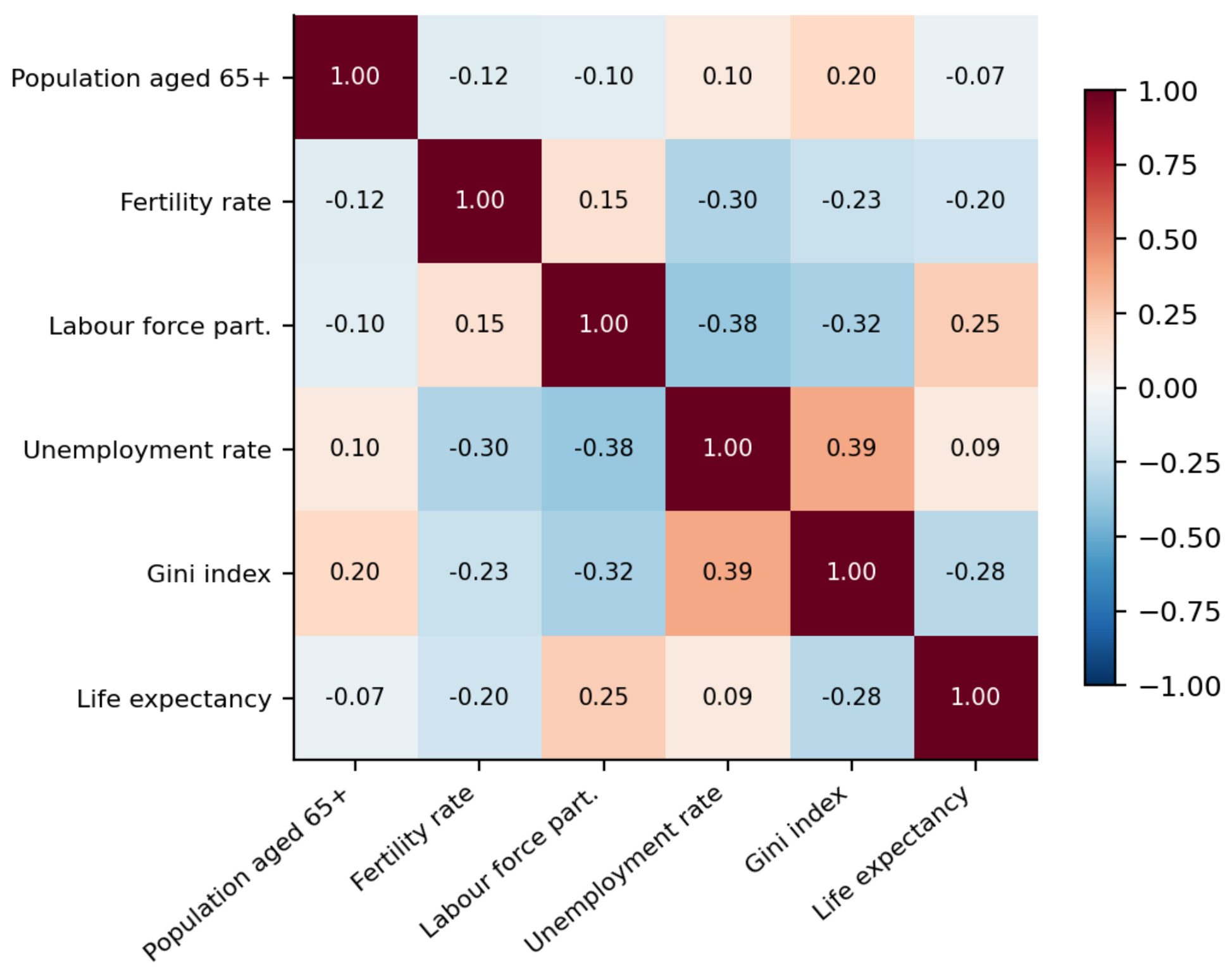
Table D3.
Correlated random effects estimates (Mundlak), social block.
| Variable | Within coefficient | Country mean |
|---|---|---|
| Population aged 65+ | 0.0446** | −0.0633* |
| Fertility rate | −0.0696 | 0.2079 |
| Labour force participation | 0.0112 | −0.0060 |
| Unemployment rate | −0.0143* | −0.0213 |
| Gini index | −0.0034 | 0.0355** |
| Life expectancy | −0.0227** | 0.0949*** |
Note. Joint Wald test on the country means: χ2(6) = 33.91, p < 0.001. N = 270.
Table D4.
Fixed-effects estimates with Driscoll–Kraay standard errors, social block.
| Variable | Coefficient | DK standard error | p-value |
|---|---|---|---|
| Population aged 65+ | 0.0446 | 0.0109 | 0.000 |
| Fertility rate | −0.0696 | 0.0495 | 0.161 |
| Labour force participation | 0.0112 | 0.0012 | 0.000 |
| Unemployment rate | −0.0143 | 0.0021 | 0.000 |
| Gini index | −0.0034 | 0.0080 | 0.674 |
| Life expectancy | −0.0227 | 0.0076 | 0.003 |
| Variable | Coefficient | Standard error | p-value |
| Population aged 65+ | 0.0401 | 0.0218 | 0.068 |
| Fertility rate | −0.0431 | 0.1304 | 0.741 |
| Labour force participation | 0.0061 | 0.0069 | 0.379 |
| Unemployment rate | −0.0140 | 0.0075 | 0.063 |
| Gini index | −0.0009 | 0.0086 | 0.921 |
| Life expectancy | −0.0208 | 0.0087 | 0.018 |
| GDP per capita (log) | 0.1280 | 0.1220 | 0.295 |
| Note. Fixed effects, N = 270, R2 = 0.468, clustered standard errors. | |||
Table D5.
Fixed effects controlling for income, social block.
| Variable | Coefficient | t statistic | p, clustered | p, bootstrap |
|---|---|---|---|---|
| Population aged 65+ | 0.0446 | 2.10 | 0.025 | 0.047 |
| Life expectancy | −0.0227 | −2.29 | 0.015 | 0.042 |
| Unemployment rate | −0.0143 | −1.80 | 0.055 | 0.120 |
| Labour force participation | 0.0112 | 1.06 | 0.254 | 0.327 |
| Fertility rate | −0.0696 | −0.45 | 0.630 | 0.688 |
| Gini index | −0.0034 | −0.32 | 0.728 | 0.769 |
Note. 1,999 replications, Rademacher weights, restricted null, G = 29 clusters.
Table D6.
Wild cluster bootstrap inference, social block.
| Variable | Anderson–Hsiao | Total packaging (FE) |
|---|---|---|
| Lagged difference/lag | 0.7486*** | — |
| Population aged 65+ | −0.0044 | 0.0364** |
| Fertility rate | 0.3852** | 0.1523 |
| Labour force participation | 0.0016 | 0.0185* |
| Unemployment rate | 0.0039 | −0.0127 |
| Gini index | −0.0138** | −0.0016 |
| Life expectancy | 0.0071 | −0.0203* |
| Observations | 212 | 270 |
| R2 | — | 0.538 |
Note. Anderson–Hsiao first-stage F statistic on the excluded instrument: 19.12. Regressors in first differences.
Figure D2.
Fixed-effects residual diagnostics.
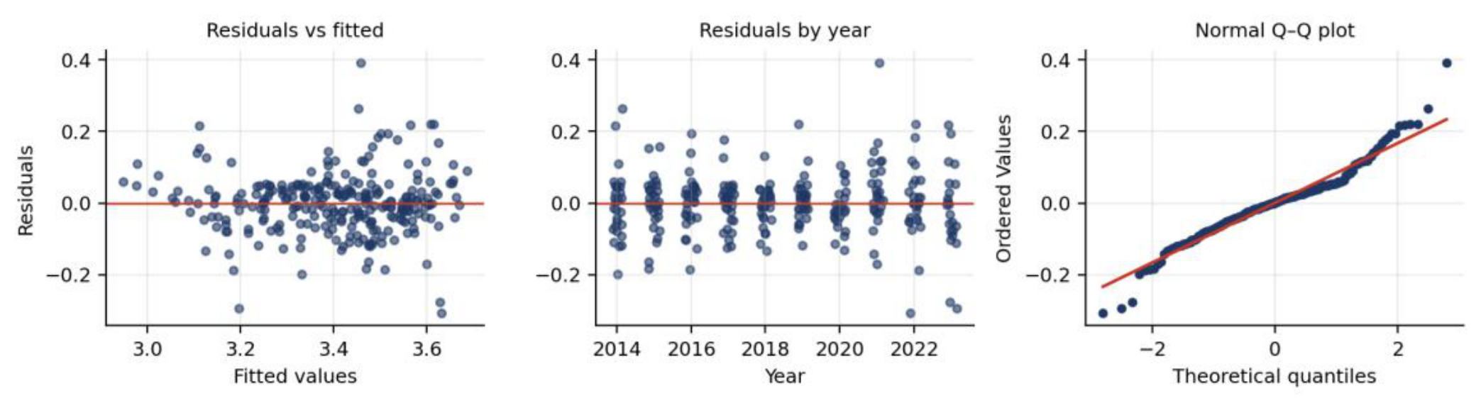
Appendix E
Table E1.
Cluster membership and silhouette widths, social block.
| Cluster | Countries | n | Mean silhouette |
|---|---|---|---|
| 1. Eastern transition | Bulgaria, Croatia, Hungary, Latvia, Lithuania, Poland, Romania | 7 | 0.279 |
| 2. Southern high-unemployment | Greece, Italy, Portugal, Spain | 4 | 0.338 |
| 3. Western and Nordic | Austria, Belgium, Cyprus, Czechia, Denmark, Estonia, Finland, France, Germany, Iceland, Ireland, Luxembourg, Malta, Netherlands, Norway, Slovak Republic, Slovenia, Sweden | 18 | 0.228 |
Figure E1.
Silhouette widths by cluster.
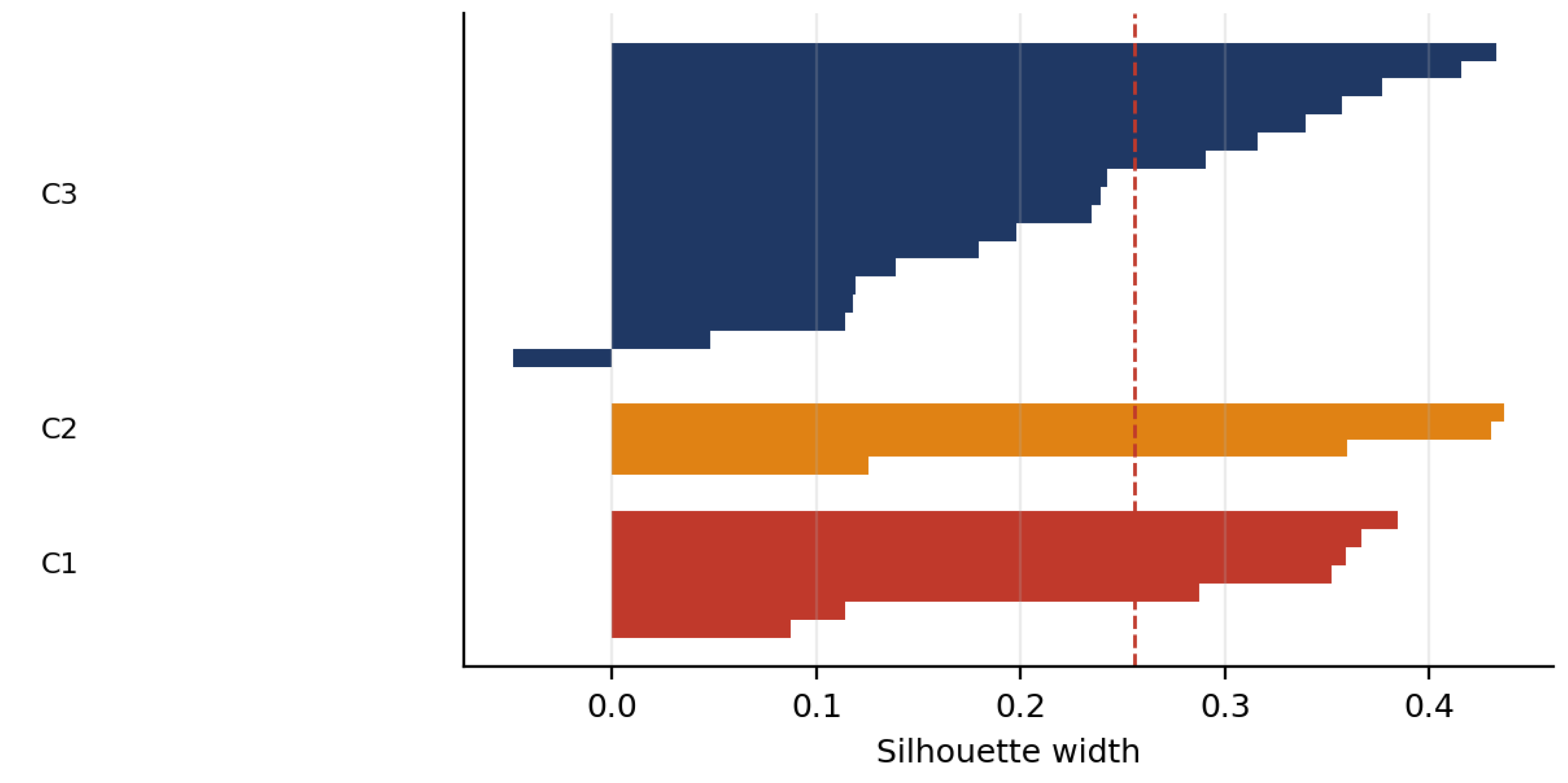
Table E2.
Number of clusters: full criteria.
| k | R2 | Silhouette | Calinski–Harabasz | Davies–Bouldin | AIC | BIC | WSS | ΔWSS |
|---|---|---|---|---|---|---|---|---|
| 2 | 0.259 | 0.238 | 9.431 | 1.589 | 469.66 | 488.81 | 128.96 | — |
| 3 | 0.430 | 0.256 | 9.816 | 1.205 | 437.91 | 466.63 | 99.14 | 29.82 |
| 4 | 0.541 | 0.248 | 9.830 | 1.267 | 414.22 | 452.50 | 79.83 | 19.31 |
| 5 | 0.601 | 0.237 | 9.023 | 1.077 | 404.09 | 451.95 | 69.49 | 10.34 |
| 6 | 0.652 | 0.197 | 8.624 | 1.182 | 394.06 | 451.48 | 60.53 | 8.97 |
| 7 | 0.698 | 0.219 | 8.471 | 1.037 | 383.51 | 450.51 | 52.56 | 7.96 |
| 8 | 0.734 | 0.223 | 8.271 | 1.008 | 375.48 | 452.05 | 46.31 | 6.25 |
Table E3.
Cluster profiles in original units.
| Cluster | Age 65+ (%) | Fertility | Labour force part. (%) | Unemployment (%) | Gini | Life expectancy (years) | Plastic generation (kg/capita) |
|---|---|---|---|---|---|---|---|
| 1. Eastern transition | 19.24 | 1.548 | 70.94 | 7.07 | 33.75 | 75.80 | 22.9 |
| 2. Southern high-unemployment | 21.60 | 1.315 | 70.30 | 13.53 | 34.59 | 82.20 | 32.0 |
| 3. Western and Nordic | 18.12 | 1.569 | 76.73 | 6.02 | 29.03 | 81.23 | 32.7 |
Note. Generation reported as the exponential of the cluster mean of the logarithm.
Table E4.
Analysis of variance by indicator.
| Variable | F(2, 26) | p-value |
|---|---|---|
| Life expectancy | 36.290 | 0.000 |
| Unemployment rate | 15.971 | 0.000 |
| Gini index | 11.314 | 0.000 |
| Labour force participation | 5.855 | 0.008 |
| Fertility rate | 5.368 | 0.011 |
| Population aged 65+ | 3.790 | 0.036 |
| Plastic generation (log), withheld | 4.223 | 0.026 |
Table E5.
Principal component loadings.
| Variable | PC1 (38.2%) | PC2 (22.0%) |
|---|---|---|
| Population aged 65+ | 0.356 | −0.087 |
| Fertility rate | −0.389 | −0.459 |
| Labour force participation | −0.471 | 0.190 |
| Unemployment rate | 0.496 | 0.334 |
| Gini index | 0.480 | −0.222 |
| Life expectancy | −0.153 | 0.765 |
Appendix F
Table F1.
Hyperparameters and protocol.
| Algorithm | Configuration |
|---|---|
| Linear regression | Ordinary least squares on standardised predictors |
| Linear SVM | ε-insensitive regression, C = 1.0, ε = 0.05, 50,000 iterations |
| K-nearest neighbours | k = 5, distance weighting, standardised predictors |
| Decision tree | Maximum depth 4, minimum leaf size 5 |
| Random forest | 800 trees, minimum leaf size 2 |
| Boosting | 500 stages, learning rate 0.03, maximum depth 3, subsample 0.8 |
Table F2.
Within-transformed results in full.
| Algorithm | R2 | RMSE | MAE | Correlation | Median AE | Mean rank |
|---|---|---|---|---|---|---|
| Linear SVM | 0.376 | 0.091 | 0.066 | 0.619 | 0.047 | 1.4 |
| Linear regression | 0.362 | 0.092 | 0.066 | 0.606 | 0.046 | 2.0 |
| K-nearest neighbours | 0.332 | 0.095 | 0.068 | 0.579 | 0.048 | 3.6 |
| Decision tree | 0.328 | 0.095 | 0.068 | 0.601 | 0.051 | 3.8 |
| Random forest | 0.295 | 0.097 | 0.070 | 0.557 | 0.046 | 4.2 |
| Boosting | 0.230 | 0.101 | 0.074 | 0.531 | 0.052 | 6.0 |
The mean absolute percentage error is not reported because the demeaned dependent variable takes values arbitrarily close to zero. The within-transformed exercise achieves higher accuracy than the levels exercise for every algorithm, which reflects the removal of the permanent country component rather than a better model.
Table F3.
Standardised coefficients and importance compared.
| Variable | FE standardised |β| | Between standardised |β| | Pooled standardised |β| |
|---|---|---|---|
| Life expectancy | 0.199 | 0.632 | 0.607 |
| Unemployment rate | 0.176 | 0.440 | 0.434 |
| Gini index | 0.039 | 0.371 | 0.348 |
| Population aged 65+ | 0.361 | 0.152 | 0.090 |
| Labour force participation | 0.186 | 0.086 | 0.126 |
| Fertility rate | 0.040 | 0.078 | 0.059 |
Figure F1.
Observed versus cross-validated predictions.
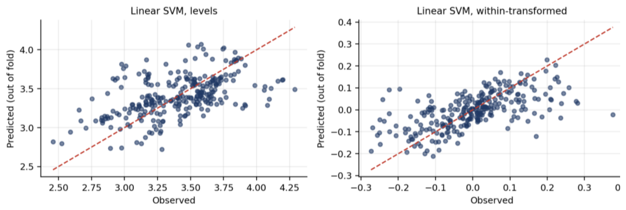
Figure F1.
Partial dependence, random forest on within-transformed data.
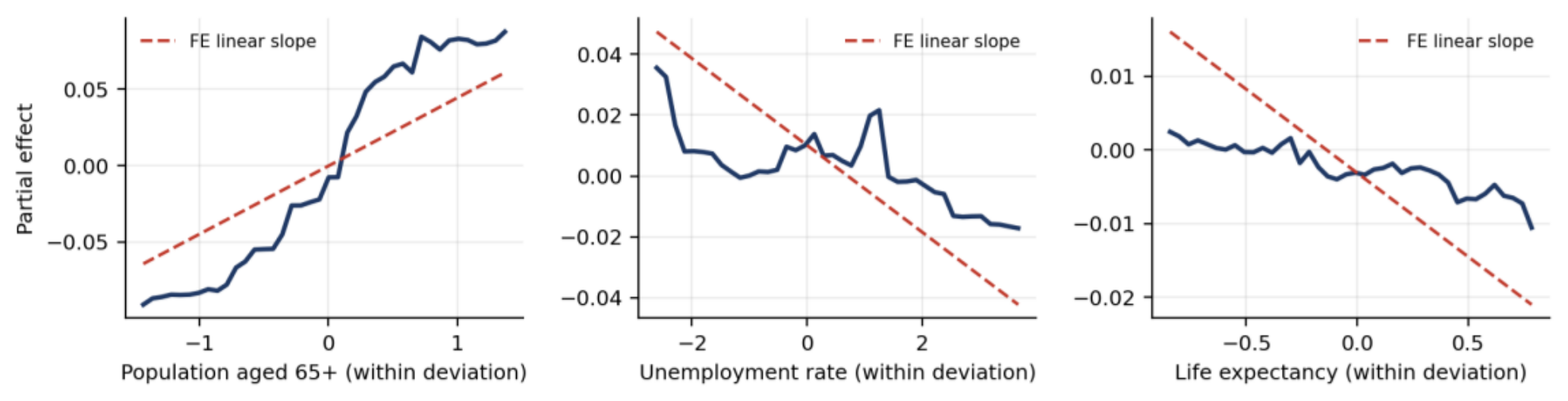
Appendix G
Table G1.
Descriptive statistics and variance decomposition.
| Variable | Mean | SD | Min | Median | Max | SD between | SD within | Within share |
|---|---|---|---|---|---|---|---|---|
| Plastic generation, log | 3.413 | 0.327 | 2.459 | 3.450 | 4.290 | 0.312 | 0.118 | 0.275 |
| GDP growth (%) | 2.761 | 3.758 | −10.940 | 2.576 | 24.624 | 1.705 | 3.357 | 0.663 |
| Net migration (log) | 6.355 | 7.780 | −11.985 | 9.501 | 13.977 | 6.030 | 5.114 | 0.459 |
| Internet users (%) | 84.602 | 10.131 | 54.078 | 86.308 | 99.687 | 8.761 | 5.513 | 0.386 |
| Women in parliament (%) | 29.992 | 10.168 | 10.050 | 30.301 | 47.619 | 9.681 | 3.481 | 0.264 |
| Institutional quality (PC1) | −0.082 | 2.251 | −4.839 | −0.285 | 3.640 | 2.295 | 0.293 | 0.113 |
| R&D expenditure (% GDP) | 1.704 | 0.873 | 0.382 | 1.449 | 3.600 | 0.867 | 0.154 | 0.151 |
Table G2.
Correlation matrix and collinearity.
| Variable | GDP growth | Migration | Internet | Women in parl. | Inst. quality | R&D | VIF |
|---|---|---|---|---|---|---|---|
| GDP growth | 1.000 | −0.049 | −0.045 | −0.260 | −0.102 | −0.239 | 1.10 |
| Net migration (log) | −0.049 | 1.000 | 0.513 | 0.379 | 0.527 | 0.478 | 1.52 |
| Internet users | −0.045 | 0.513 | 1.000 | 0.517 | 0.750 | 0.492 | 2.46 |
| Women in parliament | −0.260 | 0.379 | 0.517 | 1.000 | 0.628 | 0.728 | 2.40 |
| Institutional quality | −0.102 | 0.527 | 0.750 | 0.628 | 1.000 | 0.677 | 3.32 |
| R&D expenditure | −0.239 | 0.478 | 0.492 | 0.728 | 0.677 | 1.000 | 2.74 |
Figure G1.
Correlation matrix, governance block.
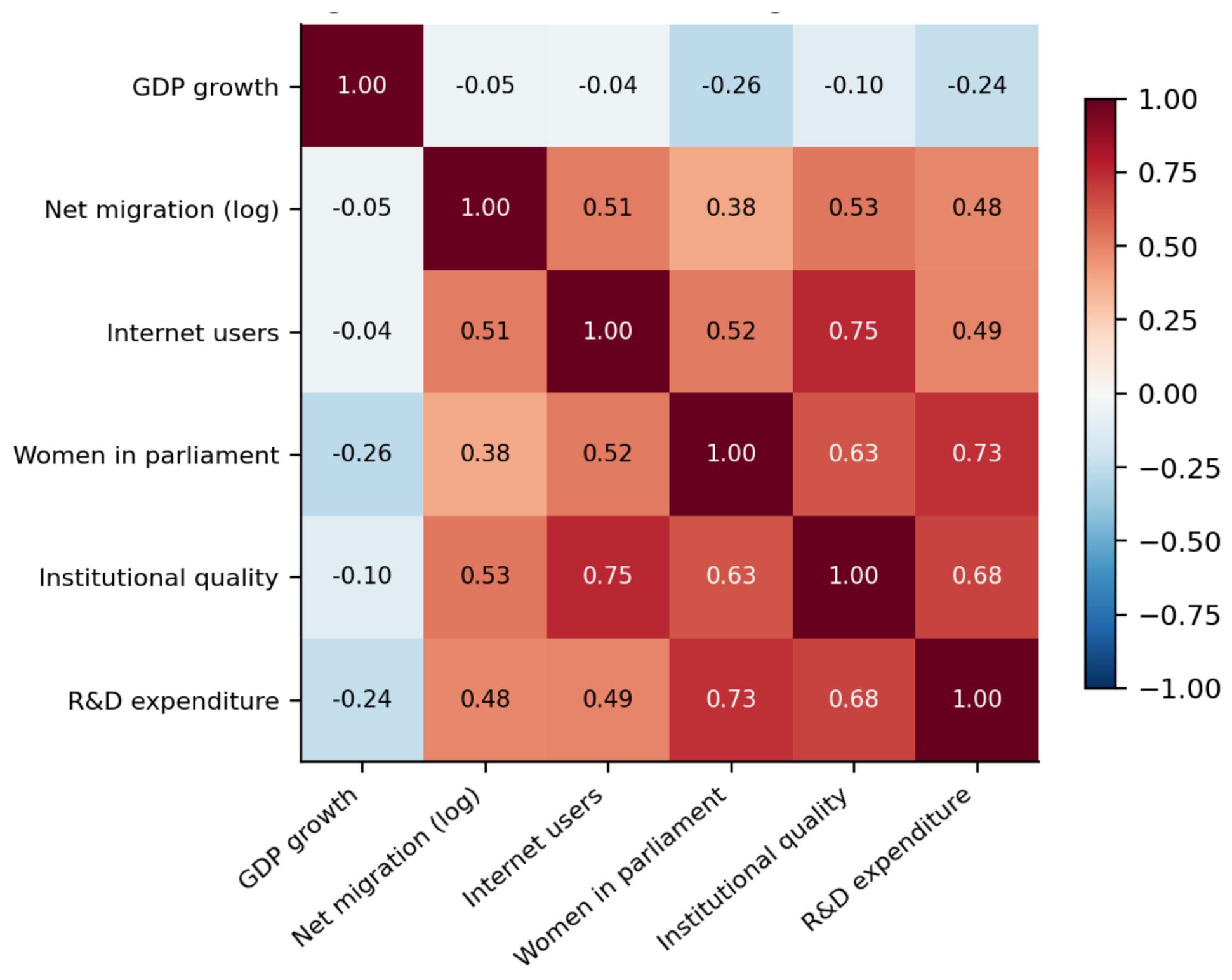
Table G3.
Correlated random effects and income control.
| Variable | Within coefficient | Country mean | With GDP per capita |
|---|---|---|---|
| GDP growth | 0.0041*** | 0.0377 | 0.0038** |
| Net migration (log) | 0.0011 | 0.0281*** | 0.0010 |
| Internet users | 0.0127*** | −0.0112 | 0.0114*** |
| Women in parliament | 0.0027 | 0.0058 | 0.0021 |
| Institutional quality | 0.0151 | 0.0230 | 0.0148 |
| R&D expenditure | 0.0278 | −0.1531 | 0.0274 |
| GDP per capita (log) | — | — | 0.0868 |
Note. Mundlak joint Wald test on the country means: χ2(6) = 18.80, p = 0.005. Third column: fixed effects with income, N = 282, R2 = 0.470.
Table G4.
Wild cluster bootstrap inference.
| Variable | Coefficient | t statistic | p, clustered | p, bootstrap |
|---|---|---|---|---|
| Internet users | 0.0127 | 5.58 | 0.000 | 0.0005 |
| GDP growth | 0.0041 | 2.86 | 0.002 | 0.0120 |
| Women in parliament | 0.0027 | 1.24 | 0.187 | 0.2270 |
| Net migration (log) | 0.0011 | 0.60 | 0.522 | 0.5970 |
| Institutional quality | 0.0151 | 0.46 | 0.625 | 0.6510 |
| R&D expenditure | 0.0278 | 0.37 | 0.693 | 0.7175 |
Note. 1,999 replications, Rademacher weights, restricted null, G = 29 clusters.
Table G5.
The six governance indicators individually.
| Indicator | Coefficient | p-value | R2 |
|---|---|---|---|
| Rule of law | 0.1242 | 0.235 | 0.472 |
| Political stability | 0.1149 | 0.111 | 0.479 |
| Control of corruption | −0.0018 | 0.989 | 0.464 |
| Regulatory quality | −0.0107 | 0.885 | 0.464 |
| Government effectiveness | −0.0294 | 0.708 | 0.465 |
| Voice and accountability | −0.0703 | 0.578 | 0.466 |
Note. Each indicator replaces the composite index in the fixed-effects specification; all other regressors unchanged. N = 282.
Table G6.
Dynamic robustness and the packaging aggregate.
| Variable | Anderson–Hsiao | Total packaging (FE) |
|---|---|---|
| Lagged difference/lag | 0.9258*** | — |
| GDP growth | 0.0048*** | 0.0034*** |
| Net migration (log) | −0.0021** | −0.0008 |
| Internet users | −0.0045* | 0.0126*** |
| Women in parliament | 0.0025 | 0.0025 |
| Institutional quality | 0.0426 | 0.0436* |
| R&D expenditure | 0.0592 | 0.0308 |
| Observations | 224 | 282 |
| R2 | — | 0.582 |
Note. Anderson–Hsiao first-stage F statistic on the excluded instrument: 19.70. Regressors in first differences.
Figure G2.
Fixed-effects residual diagnostics.
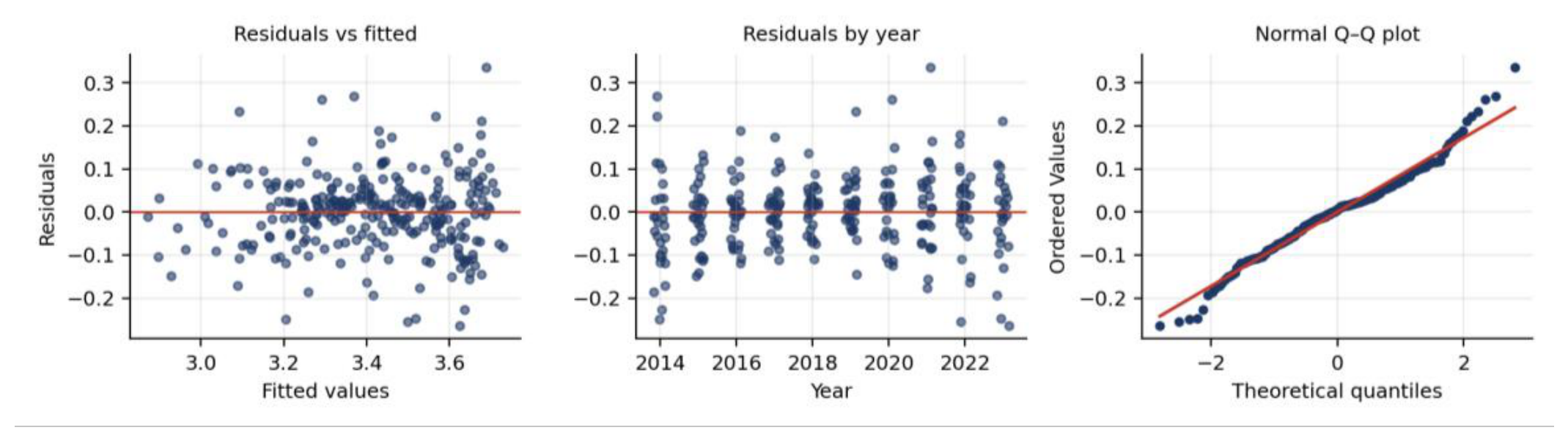
Appendix H
Table H1.
Cluster membership.
| Cluster | Countries | n | Mean silhouette |
|---|---|---|---|
| 1. Institutionally strong | Austria, Belgium, Denmark, Estonia, Finland, France, Germany, Iceland, Luxembourg, Netherlands, Norway, Slovenia, Spain, Sweden | 14 | 0.460 |
| 2. Eastern and southern | Bulgaria, Croatia, Czechia, Greece, Italy, Latvia, Lithuania, Poland, Portugal, Romania, Slovak Republic | 11 | 0.266 |
| 3. High-growth small economies | Cyprus, Hungary, Ireland, Malta | 4 | 0.339 |
Figure H1.
Silhouette widths by cluster.
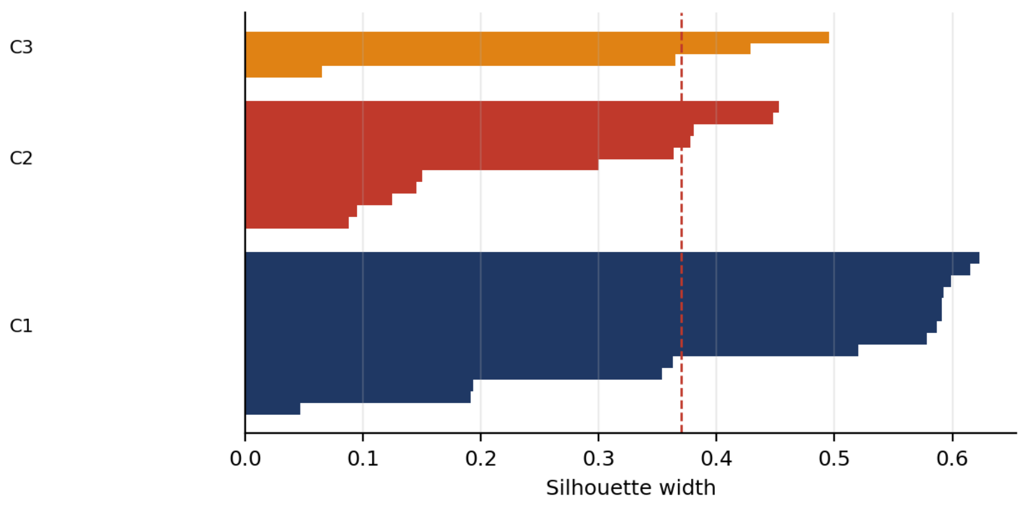
Table H2.
Number of clusters: full criteria.
| k | R2 | Silhouette | Calinski–Harabasz | Davies–Bouldin | AIC | BIC | WSS | ΔWSS |
|---|---|---|---|---|---|---|---|---|
| 2 | 0.494 | 0.387 | 26.397 | 0.924 | 403.14 | 422.28 | 87.98 | — |
| 3 | 0.622 | 0.370 | 21.372 | 0.974 | 366.61 | 395.33 | 65.81 | 22.17 |
| 4 | 0.734 | 0.349 | 23.046 | 0.948 | 319.08 | 357.37 | 46.21 | 19.60 |
| 5 | 0.778 | 0.317 | 21.008 | 1.023 | 302.03 | 349.89 | 38.66 | 7.55 |
| 6 | 0.814 | 0.272 | 20.170 | 1.043 | 284.85 | 342.27 | 32.31 | 6.34 |
| 7 | 0.841 | 0.270 | 19.353 | 0.992 | 272.14 | 339.14 | 27.71 | 4.60 |
| 8 | 0.862 | 0.256 | 18.723 | 0.865 | 261.31 | 337.88 | 24.03 | 3.68 |
Table H3.
Cluster profiles in original units.
| Cluster | GDP growth (%) | Net migration (log) | Internet users (%) | Women in parl. (%) | Inst. quality (PC1) | R&D (% GDP) | Plastic generation (kg/capita) |
|---|---|---|---|---|---|---|---|
| 1. Institutionally strong | 1.92 | 9.76 | 90.96 | 37.55 | 1.582 | 2.361 | 34.2 |
| 2. Eastern and southern | 2.78 | 0.47 | 75.98 | 24.87 | −2.131 | 1.086 | 24.5 |
| 3. High-growth small economies | 5.55 | 9.35 | 83.85 | 16.21 | −0.838 | 0.975 | 34.2 |
Note. Generation reported as the exponential of the cluster mean of the logarithm.
Table H4.
Analysis of variance and the two-cluster alternative.
| Variable | F(2, 26) | p-value |
|---|---|---|
| Women in parliament | 30.850 | 0.000 |
| Internet users | 23.653 | 0.000 |
| GDP growth | 21.874 | 0.000 |
| Institutional quality | 19.019 | 0.000 |
| R&D expenditure | 18.760 | 0.000 |
| Net migration | 17.228 | 0.000 |
| Plastic generation (log), withheld | 5.268 | 0.012 |
Table H5.
Principal component loadings.
| Variable | PC1 (64.5%) | PC2 (18.5%) |
|---|---|---|
| GDP growth | −0.279 | 0.727 |
| Net migration (log) | 0.387 | 0.337 |
| Internet users | 0.417 | 0.386 |
| Women in parliament | 0.431 | −0.305 |
| Institutional quality | 0.461 | 0.280 |
| R&D expenditure | 0.447 | −0.193 |
Appendix I
Table I1.
Hyperparameters and protocol.
| Algorithm | Configuration |
|---|---|
| Linear regression | Ordinary least squares on standardised predictors |
| Linear SVM | ε-insensitive regression, C = 1.0, ε = 0.05, 50,000 iterations |
| K-nearest neighbours | k = 5, distance weighting, standardised predictors |
| Decision tree | Maximum depth 4, minimum leaf size 5 |
| Random forest | 800 trees, minimum leaf size 2 |
| Boosting | 500 stages, learning rate 0.03, maximum depth 3, subsample 0.8 |
Table I2.
Within-transformed results in full.
| Algorithm | R2 | RMSE | MAE | Correlation | Median AE | Mean rank |
|---|---|---|---|---|---|---|
| Linear SVM | 0.374 | 0.094 | 0.071 | 0.621 | 0.057 | 1.4 |
| Linear regression | 0.372 | 0.094 | 0.070 | 0.615 | 0.056 | 1.6 |
| Random forest | 0.349 | 0.095 | 0.072 | 0.605 | 0.057 | 3.0 |
| Boosting | 0.298 | 0.099 | 0.077 | 0.577 | 0.063 | 4.0 |
| K-nearest neighbours | 0.269 | 0.101 | 0.080 | 0.541 | 0.066 | 5.2 |
| Decision tree | 0.210 | 0.105 | 0.080 | 0.525 | 0.064 | 5.8 |
Table I3.
Standardised coefficients compared with importance.
| Variable | FE standardised |β| | Between standardised |β| | Pooled standardised |β| |
|---|---|---|---|
| Net migration (log) | 0.026 | 0.695 | 0.317 |
| GDP growth | 0.047 | 0.481 | 0.115 |
| R&D expenditure | 0.074 | 0.335 | 0.239 |
| Women in parliament | 0.084 | 0.264 | 0.110 |
| Institutional quality | 0.104 | 0.263 | 0.313 |
| Internet users | 0.394 | 0.045 | 0.224 |
Figure IA.
Observed versus cross-validated predictions.
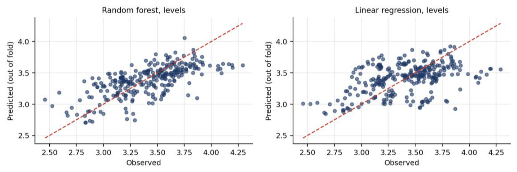
Table I5.
Comparison across the three pillars.
| Pillar | Best in levels | R2 | Best within | R2 | Verdict on linearity |
|---|---|---|---|---|---|
| Environmental | Linear regression | 0.191 | K-nearest neighbours | 0.398 | Adequate between, mild non-linearity within |
| Social | Linear SVM | 0.172 | Linear SVM | 0.376 | Adequate in both dimensions |
| Governance | Random forest | 0.445 | Linear SVM | 0.374 | Inadequate between, adequate within |
References
- Ahmed, S.; et al. Is economic growth still driving municipal waste? Evidence from European Union and Western Balkan Countries. In Waste Management and Research; 2026. [Google Scholar] [CrossRef]
- Akther, A.; et al. Municipal solid waste dynamics: Economic, environmental, and technological determinants in Europe. Clean. Eng. Technol. 2025, 21. [Google Scholar] [CrossRef]
- Antanasijević, D.; et al. The forecasting of municipal waste generation using artificial neural networks and sustainability indicators. Sustain. Sci. 2013, 8. [Google Scholar] [CrossRef]
- Antczak, E. Municipal Waste in Poland: Analysis of the Spatial Dimensions of Determinants Using Geographically Weighted Regression. Eur. Spat. Res. Policy 2019, 26. [Google Scholar] [CrossRef]
- Arbulú, I.; et al. Tourism and solid waste generation in Europe: A panel data assessment of the Environmental Kuznets Curve. Waste Manag. 2015, 46. [Google Scholar] [CrossRef]
- Avilés-Palacios, C.; Rodríguez-Olalla, A. The sustainability of waste management models in circular economies. Sustainability 2021, 13. [Google Scholar]
- Banacu, C. S.; et al. Entrepreneurial innovation impact on recycling municipal waste. A panel data analysis at the EU level. Sustainability 2019, 11. [Google Scholar] [CrossRef]
- Bassem, B. S. Digitalisation and waste-to-energy development: Nonlinear and dynamic evidence from the European Union; 2026. [Google Scholar]
- Bodislav, D. A.; et al. The Opportunity Cost Between the Circular Economy and Economic Growth: Clustering the Approaches. In Sustainability (Switzerland); 2025. [Google Scholar]
- Cehlár, M.; et al. Municipal waste recycling in the EU: a multi-method analysis of determinants and country profiles (2005–2023). In Frontiers in Environmental Science; 2025. [Google Scholar] [CrossRef]
- Chakraborty, S. K.; et al. Municipal Solid Waste generation dynamics. Breaks and thresholds analysis in the Italian context. Waste Manag. 2022, 152. [Google Scholar] [CrossRef]
- Chalak, A.; et al. The global economic and regulatory determinants of household food waste generation: A cross-country analysis. Waste Manag. 2016, 48. [Google Scholar] [CrossRef]
- Chen, C.-C.; Chang, Y.-S. Leveraging Circular Economy Metrics for Data-Driven Forecasting of Solid Waste Production in Europe; 2024. [Google Scholar]
- Cimpan, C.; et al. Plastic packaging flows in Europe: A hybrid input-output approach. J. Ind. Ecol. 2021, 25. [Google Scholar] [CrossRef]
- Cimpan, C.; et al. Effects of Circularity Interventions in the European Plastic Packaging Sector. Environ. Sci. Technol. 2023, 57. [Google Scholar] [CrossRef]
- Clement, L.; Spinler, S. Advancing sustainability in e-commerce packaging: A simulation-based study for managing returnable systems. 2025. [Google Scholar] [CrossRef]
- Colelli, F. P.; et al. Assessment of the effectiveness and efficiency of packaging waste EPR schemes in Europe. Waste Manag. 2022, 148. [Google Scholar] [CrossRef]
- D’Adamo, I.; et al. Assessing the relation between waste management policies and circular economy goals. Waste Manag. 2022, 154. [Google Scholar] [CrossRef]
- Doran, N. M.; et al. Could e-commerce activities drive to climate change mitigation? Novel evidence from panel quantile regression. 2025. [Google Scholar] [CrossRef]
- Fellner, J.; et al. Potential impacts of the EU circular economy package on the utilization of secondary resources. Detritus 2018, 2. [Google Scholar] [CrossRef]
- Gardiner, R.; Hájek, P. Municipal waste generation, R&D intensity, and economic growth nexus – A case of EU regions. Waste Manag. 2020, 114. [Google Scholar] [CrossRef]
- Gencia, A. D.; Balan, I. M. Reevaluating Economic Drivers of Household Food Waste: Insights, Tools, and Implications Based on European GDP Correlations. Sustainability 2024, 16. [Google Scholar] [CrossRef]
- Guler, H.; et al. Does inflation instability urge solid waste generation? Evidence from European countries. 2025. [Google Scholar] [CrossRef]
- Hondroyiannis, G.; et al. Waste generation and macroeconomic drivers: a panel study for European countries and regions. In Management of Environmental Quality; 2024a. [Google Scholar]
- Hondroyiannis, G.; et al. Recycling rate performance and socioeconomic determinants: Evidence from aggregate and regional data across European Union countries. J. Clean. Prod. 2024b, 434. [Google Scholar] [CrossRef]
- İçen, H.; Çil, N. Investigating municipal waste Kuznets curve for 22 OECD countries. Environ. Monit. Assess. 2023, 195. [Google Scholar] [CrossRef]
- Joltreau, E. Extended Producer Responsibility, Packaging Waste Reduction and Eco-design. Environ. Resour. Econ. 2022, 83. [Google Scholar] [CrossRef]
- Jylhä, H.; et al. A novel method of accounting for plastic packaging waste. 2025. [Google Scholar] [CrossRef]
- Khatami, F.; et al. Efficiency of consumer behaviour and digital ecosystem in the generation of the plastic waste toward circular economy. J. Environ. Manag. 2023. [Google Scholar] [CrossRef]
- Koçak, E.; Bağlıtaş, H. H. The path to sustainable municipal solid waste management: Do human development, energy efficiency, and income inequality matter? Sustain. Dev. 2022, 30. [Google Scholar] [CrossRef]
- lo Storto, C. Evaluating the Eco-Efficiency of Municipal Solid Waste Management: Determinants, Paradoxes, and Trade-Offs. Urban Sci. 2025, 9. [Google Scholar] [CrossRef]
- Lombardi, M.; et al. Material flow analysis and sustainability of the Italian plastic packaging management. J. Clean. Prod. 2021, 287. [Google Scholar] [CrossRef]
- Lopez-Aguilar, J. F.; et al. A realistic material flow analysis for end-of-life plastic packaging management in Spain: Data gaps and suggestions for improvements towards effective recyclability. Sustain. Prod. Consum. 2022, 31. [Google Scholar] [CrossRef]
- Magrini, C.; et al. Municipal solid waste prevention: A review of market-based instruments in six European Union countries. Waste Manag. Res. 2020, 38. [Google Scholar] [CrossRef]
- Malek, W.; et al. How have waste management policies impacted the flow of municipal waste? An empirical analysis of 14 European countries. Waste Manag. 2023, 164. [Google Scholar] [CrossRef]
- Mazzanti, M.; Nicolli, F. Waste dynamics, decoupling and ex post policy effectiveness: Evidence from the EU15. Int. J. Glob. Environ. Issues 2011, 11. [Google Scholar] [CrossRef]
- Mazzarano, M.; et al. Non-constant income elasticities of waste generation. J. Clean. Prod. 2021, 318. [Google Scholar] [CrossRef]
- Morelli, G.; et al. The role of circular economy in EU entrepreneurship: A deep learning experiment. J. Econ. Asymmetries 2024, 30. [Google Scholar] [CrossRef]
- Nademi, Y.; Sedaghat Kalmarzi, H. Breaking the unemployment cycle using the circular economy: Sustainable jobs for sustainable futures. J. Clean. Prod. 2025. [Google Scholar] [CrossRef]
- Nikolić, R.; Rotar, L. J. The Effectiveness of Deposit–Refund Systems in Packaging Waste Management: A Panel Regression Analysis of EU Countries. In Environments; 2026. [Google Scholar] [CrossRef]
- Oguz-Ekim, P. Machine Learning Approaches for Municipal Solid Waste Generation Forecasting. Environ. Eng. Sci. 2021, 38. [Google Scholar] [CrossRef]
- Osińska, M. The determinants of municipal solid waste management efficiency in EU countries. In Economics and Environment; 2024. [Google Scholar]
- Oyewo, B.; et al. Microplastics in aquatic bodies: Assessing the role of governance mechanisms in industrial wastewater recycling; 2024. [Google Scholar]
- Pais-Magalhães, V.; et al. Scoring method of eco-efficiency using the DEA approach: evidence from European waste sectors. Environ. Dev. Sustain. 2021, 23. [Google Scholar] [CrossRef]
- Pavón Losada, J. A.; et al. Food packaging business models as drivers for sustainability in the food packaging industry. 2025. [Google Scholar] [CrossRef]
- Picuno, C.; et al. Factors shaping the recycling systems for plastic packaging waste — a comparison between Austria, Germany and the Netherlands. Sustainability 2021, 13. [Google Scholar] [CrossRef]
- Piontek, W.; et al. Will deposit-return system be effective in achieving the objectives of single use plastic directive? Econ. Environ. 2024. [Google Scholar] [CrossRef]
- Robaina, M.; et al. Circular economy in plastic waste – Efficiency analysis of European countries. Sci. Total Environ. 2020, 730. [Google Scholar]
- Rosecký, M.; et al. Predictive modelling as a tool for effective municipal waste management policy at different territorial levels. J. Environ. Manag. 2021, 291. [Google Scholar] [CrossRef]
- Ross, V.; et al. Reflexive EU environmental law: Exploring divergence in the French and German transposition of plastics provisions; 2024. [Google Scholar]
- Rubio, S.; et al. Effectiveness of extended producer responsibility policies implementation: The case of Portuguese and Spanish packaging waste systems. J. Clean. Prod. 2019, 210. [Google Scholar] [CrossRef]
- Rybová, K.; et al. Socio-demographic determinants of municipal waste generation: case study of the Czech Republic. J. Mater. Cycles Waste Manag. 2018, 20. [Google Scholar] [CrossRef]
- Sarc, R.; et al. Digitalisation and intelligent robotics in value chain of circular economy oriented waste management – A review. Waste Manag. 2019, 95. [Google Scholar] [CrossRef]
- Shah, W. U. H.; et al. The Repercussions of Economic Growth, Industrialization, Foreign Direct Investment, and Technology on Municipal Solid Waste: Evidence from OECD Economies. Sustainability 2023, 15. [Google Scholar]
- Sinha, A.; et al. The determinants of solid waste generation in the OECD: Evidence from cross-elasticity changes in a common correlated effects framework. Resour. Conserv. Recycl. 2022, 186. [Google Scholar] [CrossRef]
- Smailbegović, U.; et al. Assessing the determinants of municipal solid waste generation in Europe: A machine learning approach. Waste Manag. 2025, 195. [Google Scholar] [CrossRef]
- Streimikis, J. Circularity Performance in Benelux Economies: A Comparative Analysis; 2026. [Google Scholar]
- Szul, T.; et al. Data-Driven Feature Selection and Prediction of Municipal Waste Generation: Towards Sustainable Waste Management and Circular Economy Planning in the Slovak Republic. Sustainability 2026, 18. [Google Scholar] [CrossRef]
- Tyagi, P.; et al. Advances in barrier coatings and film technologies for achieving sustainable packaging of food products – A review. Trends Food Sci. Technol. 2021, 115. [Google Scholar] [CrossRef]
- Vardopoulos, I.; et al. Sustainable metropolitan areas perspectives through assessment of the existing waste management practices. Sustainability 2021, 13. [Google Scholar]
- Vučkovski, B. G.; et al. Circular Economy as a Driver of Sustainable Growth: Quantitative Analysis of the Role of Recycling and Secondary Raw Materials in the EU. Sustainability 2025, 17. [Google Scholar] [CrossRef]
- Wilts, H.; et al. Eco-innovations for waste prevention — Best practices, drivers and barriers. Sci. Total Environ. 2013, 461–462. [Google Scholar]
- Winterstetter, A.; et al. Country-specific assessment of mismanaged plastic packaging waste as a main contributor to marine litter in Europe. Front. Sustain. 2022, 3. [Google Scholar] [CrossRef]
- Zein, S. H. An Integrated ESG–Circular Economy Framework for Hydrogen Production from Plastic Waste: Theoretical Foundations and Applications; 2026. [Google Scholar]
- Ziółkowski, K.; Wieczyński, P. Enhancing forecast accuracy in the paper scrap sector: a comparative study of ensemble and machine learning methods. 2026. [Google Scholar] [CrossRef]
Figure 1.
Analytical framework: data sources, ESG pillar decomposition, methodological modules and principal findings. Note. Two data sources are merged at country-year level, partitioned into three ESG pillars, and each pillar is analysed through three modules sharing one dependent variable. The bottom row reports the principal finding per pillar.
Figure 1.
Analytical framework: data sources, ESG pillar decomposition, methodological modules and principal findings. Note. Two data sources are merged at country-year level, partitioned into three ESG pillars, and each pillar is analysed through three modules sharing one dependent variable. The bottom row reports the principal finding per pillar.
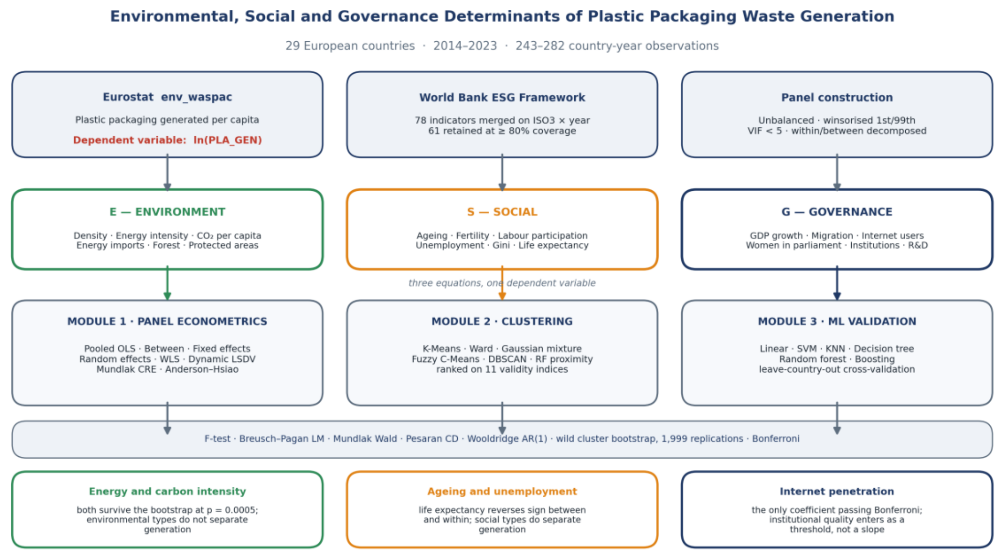
Figure 2.
Plastic packaging waste generation by country, 2014–2022.
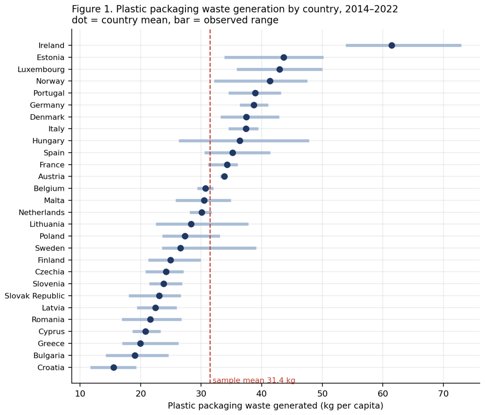
Figure 3.
Standardised coefficients across estimators, with 95% confidence intervals.
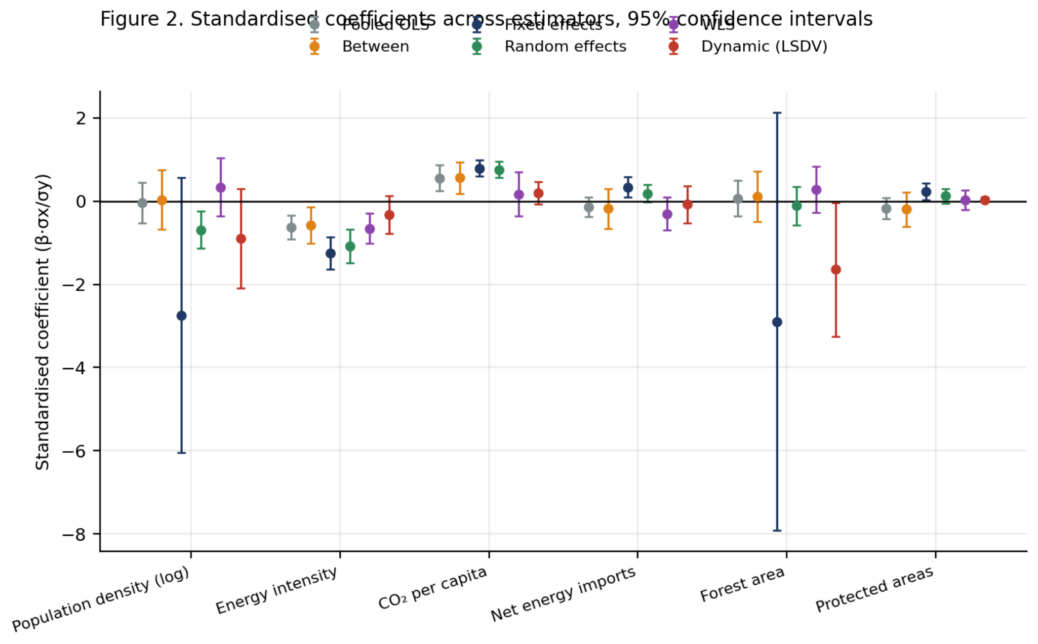
Figure 4.
Decomposition of variation: within-country share of total variation.
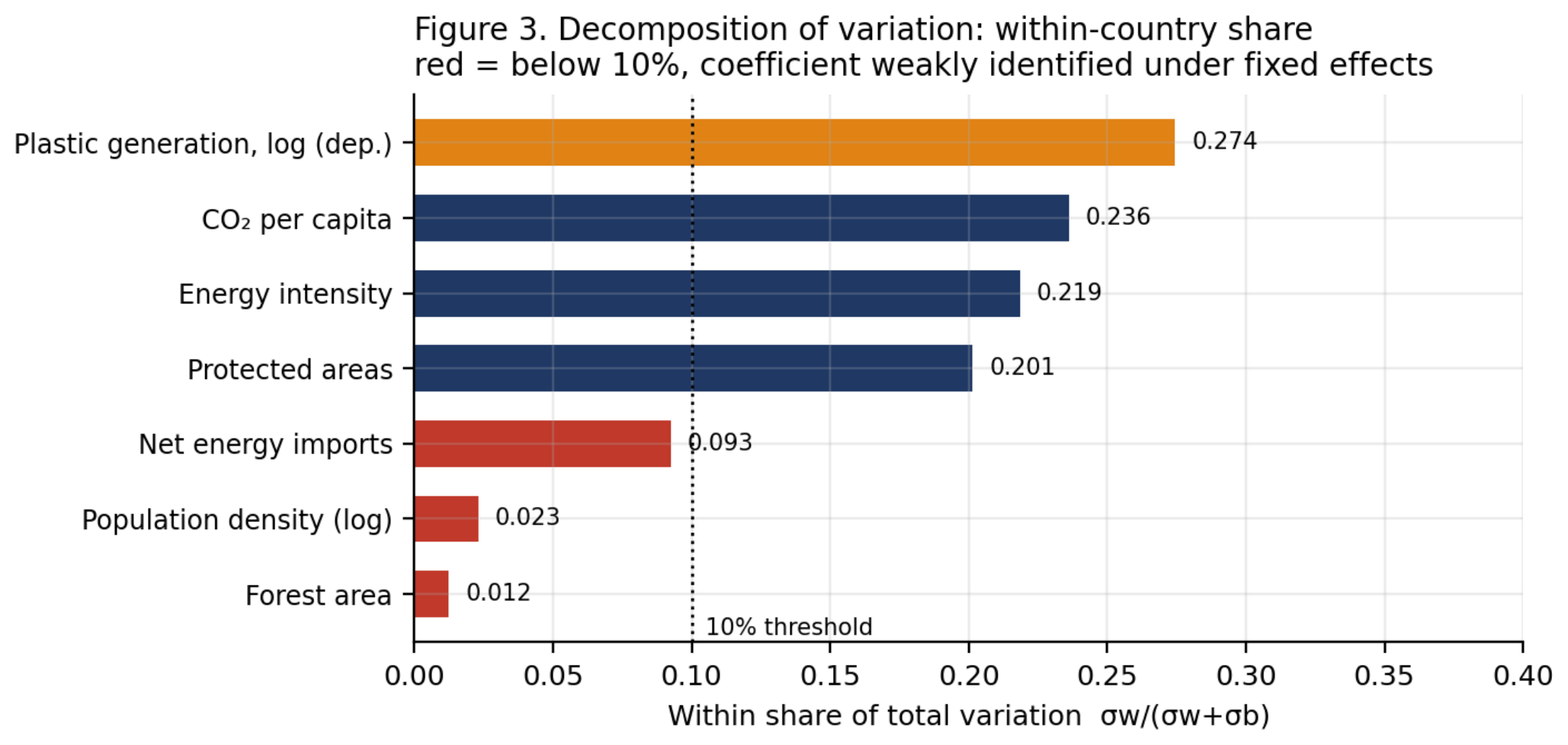
Figure 5.
Algorithm comparison by mean rank across eleven validity indices.
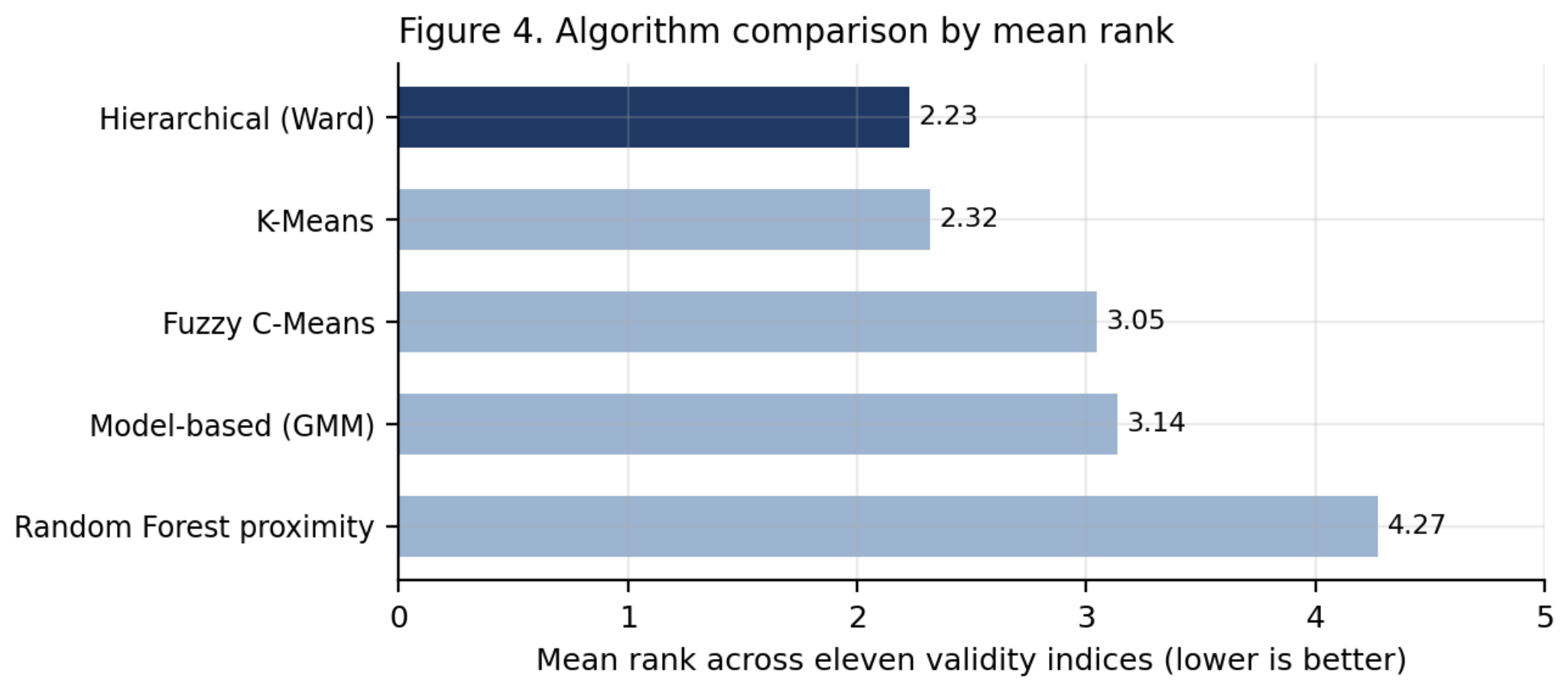
Figure 6.
Selection of the number of clusters, Ward linkage.
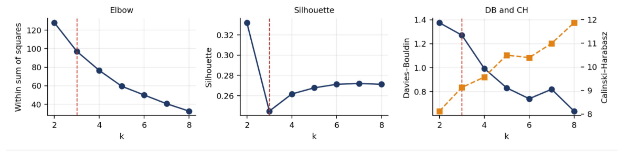
Figure 7.
Cluster membership in the space of the first two principal components.
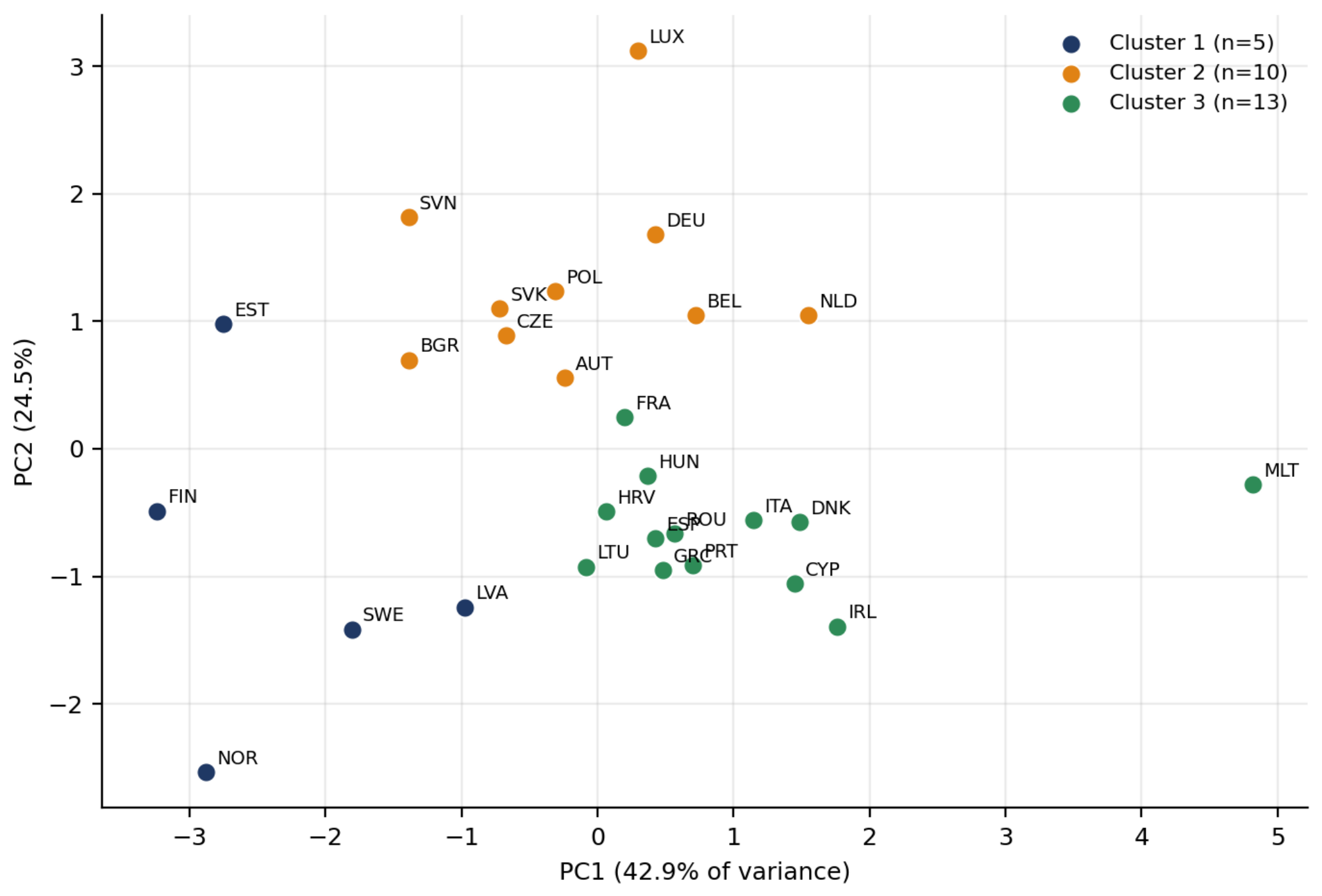
Figure 8.
Predictive performance of six algorithms, levels and within-transformed.
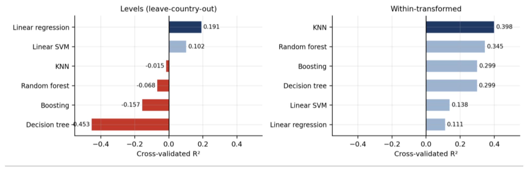
Figure 9.
Permutation importance across models and transformations.
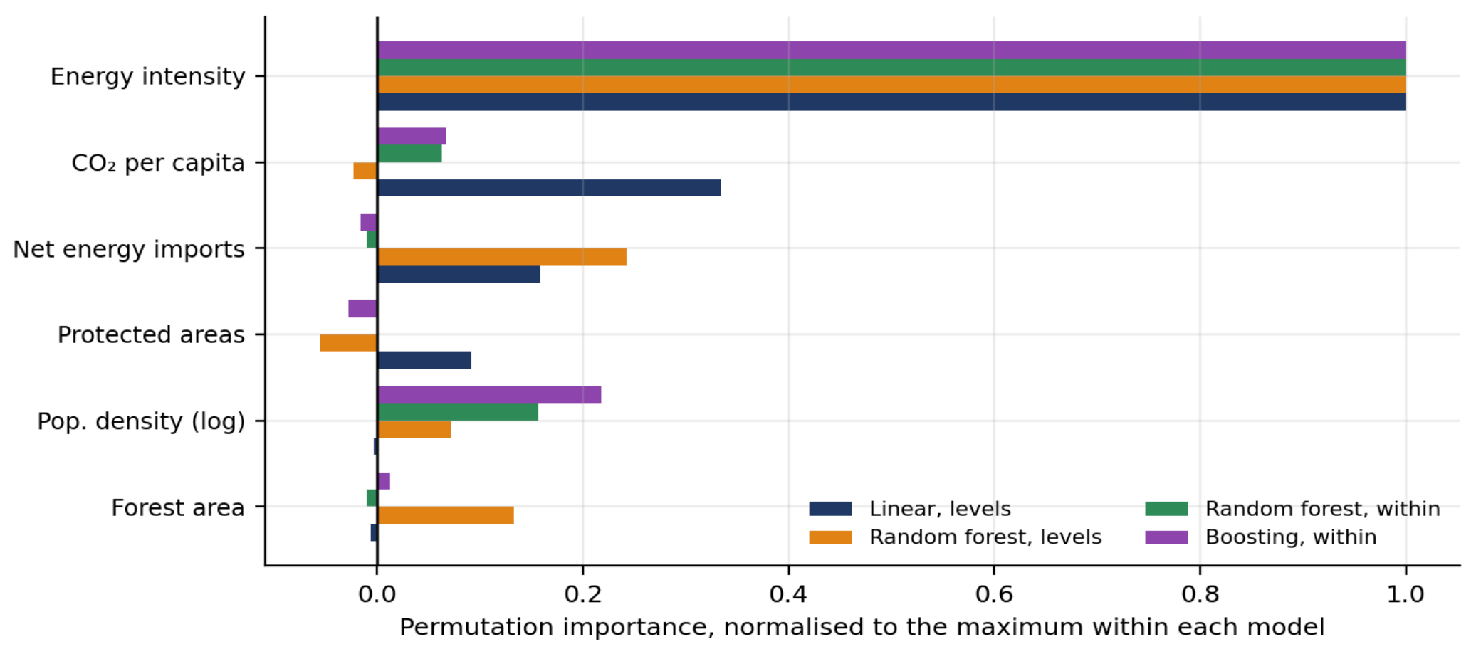
Figure 10.
Decomposition of variation: within-country share.
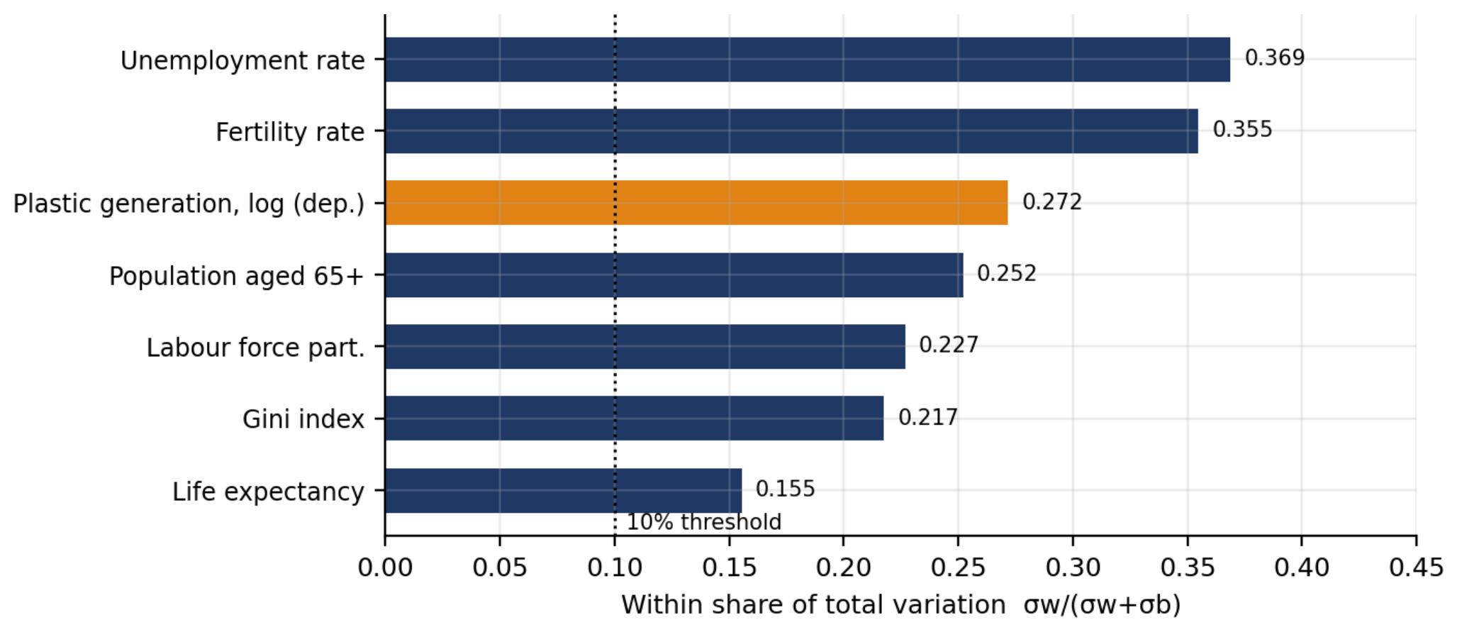
Figure 11.
Standardised coefficients across estimators, with 95% confidence intervals.
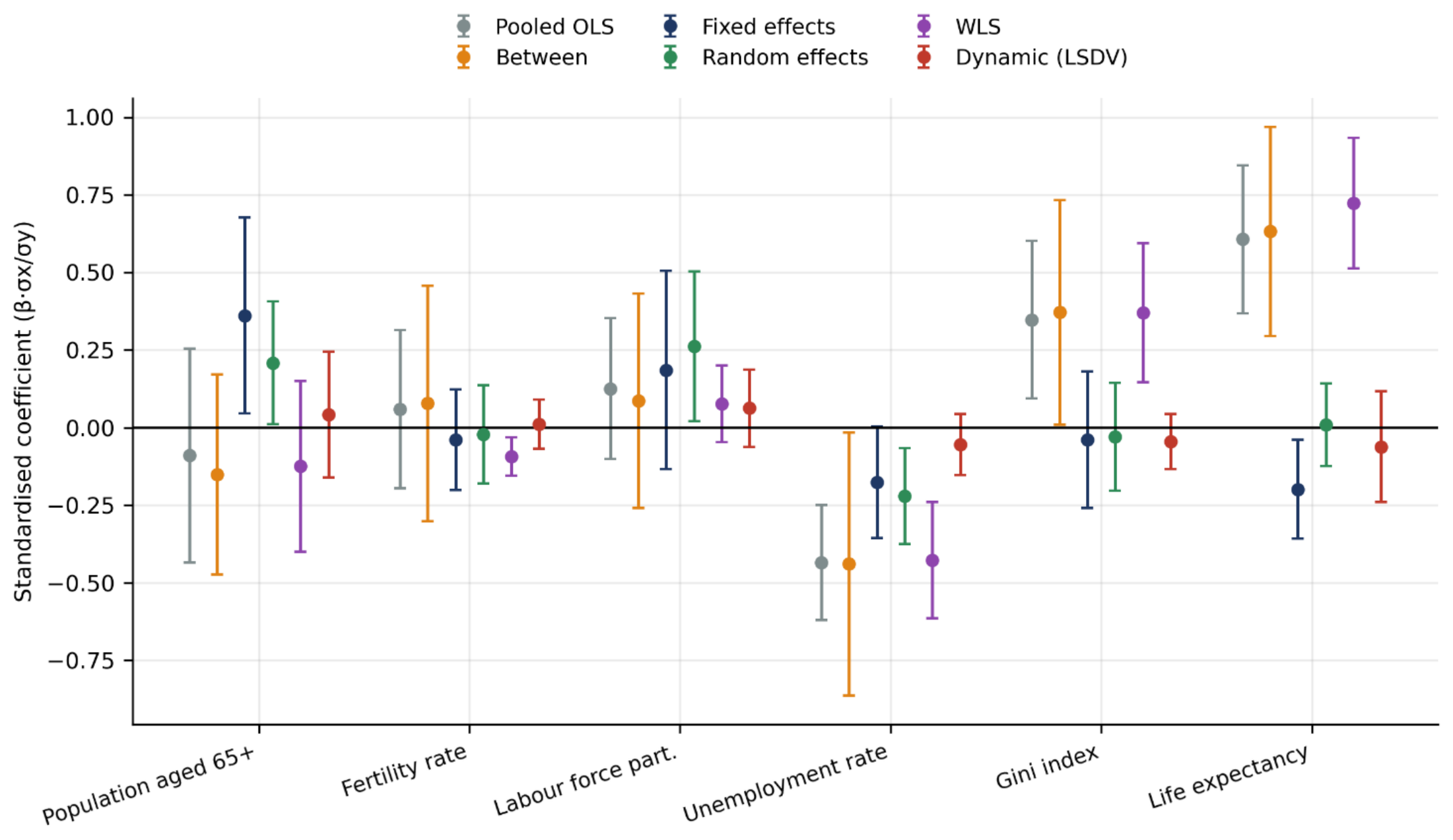
Figure 12.
Between and within relationships for the two indicators whose sign reverses.
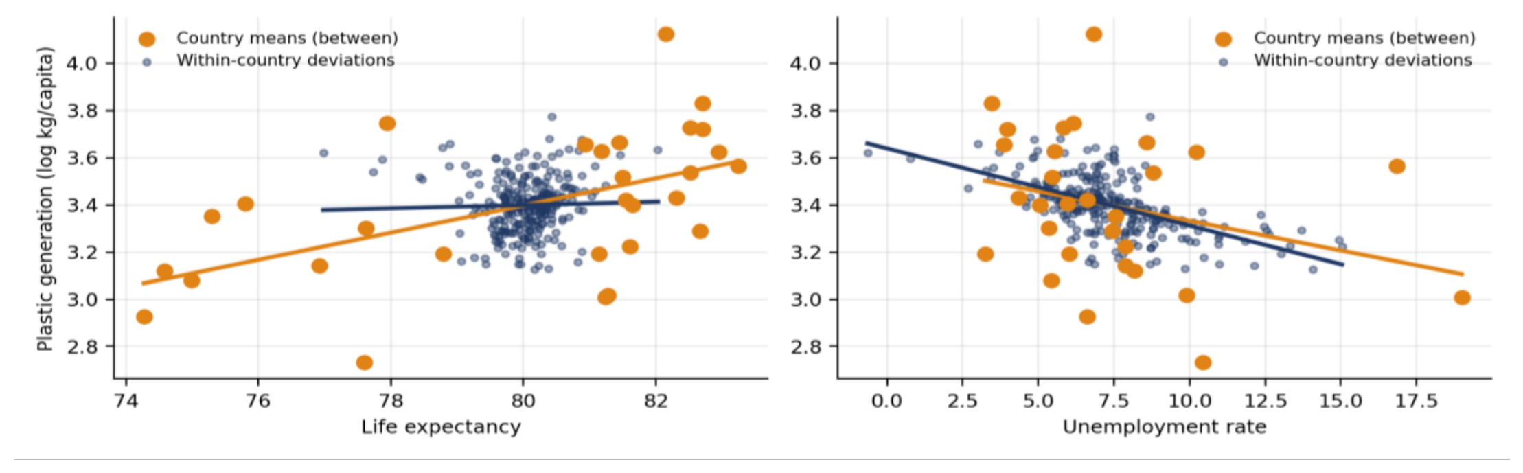
Figure 13.
Algorithm comparison by mean rank across eleven validity indices.
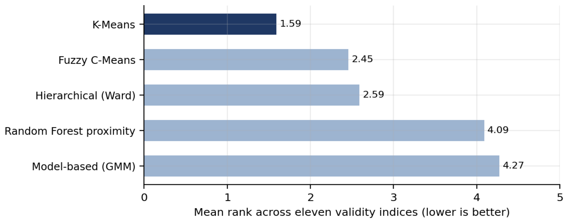
Figure 14.
Selection of the number of clusters, K-Means.
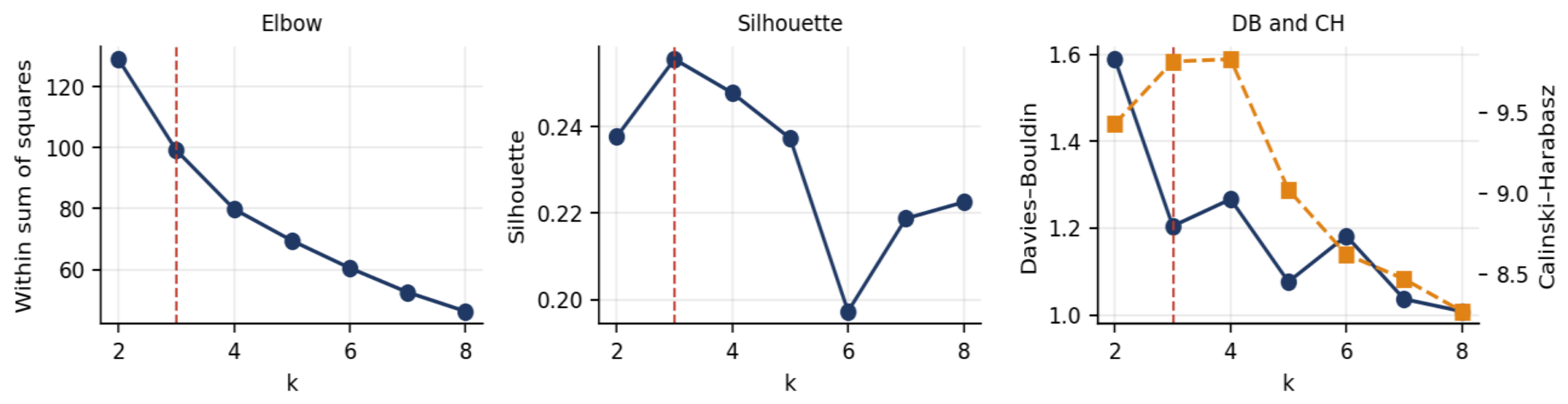
Figure 16.
Predictive performance of six algorithms, levels and within-transformed. Note. Ten-fold cross-validation grouped by country. Red bars mark negative R2, where predicting the sample mean outperforms the model. Linear methods rank first in both panels, unlike the environmental block.
Figure 16.
Predictive performance of six algorithms, levels and within-transformed. Note. Ten-fold cross-validation grouped by country. Red bars mark negative R2, where predicting the sample mean outperforms the model. Linear methods rank first in both panels, unlike the environmental block.
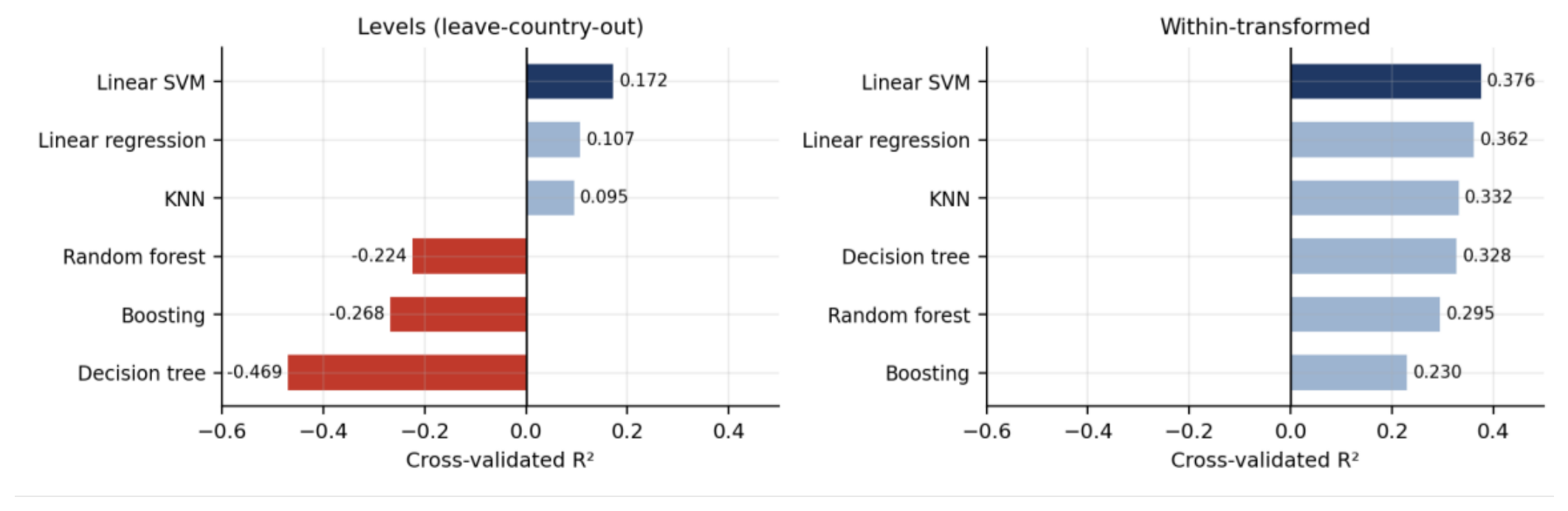
Figure 17.
Permutation importance across models and transformations. Note. Values normalised to the maximum within each model, so bars are comparable across models but not in absolute terms. Life expectancy dominates in levels, population ageing in the demeaned exercise: the hierarchy inverts.
Figure 17.
Permutation importance across models and transformations. Note. Values normalised to the maximum within each model, so bars are comparable across models but not in absolute terms. Life expectancy dominates in levels, population ageing in the demeaned exercise: the hierarchy inverts.
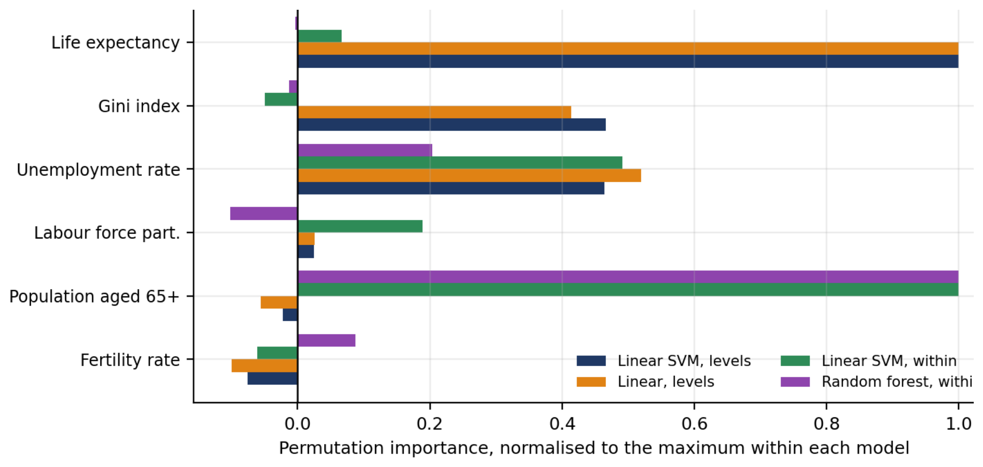
Figure 18.
Decomposition of variation: within-country share. Note. Bars show σw/(σw+σb) for each variable; the dependent variable is highlighted. GDP growth is the only regressor whose within variation exceeds its between variation. Institutional quality barely clears the ten per cent threshold.
Figure 18.
Decomposition of variation: within-country share. Note. Bars show σw/(σw+σb) for each variable; the dependent variable is highlighted. GDP growth is the only regressor whose within variation exceeds its between variation. Institutional quality barely clears the ten per cent threshold.
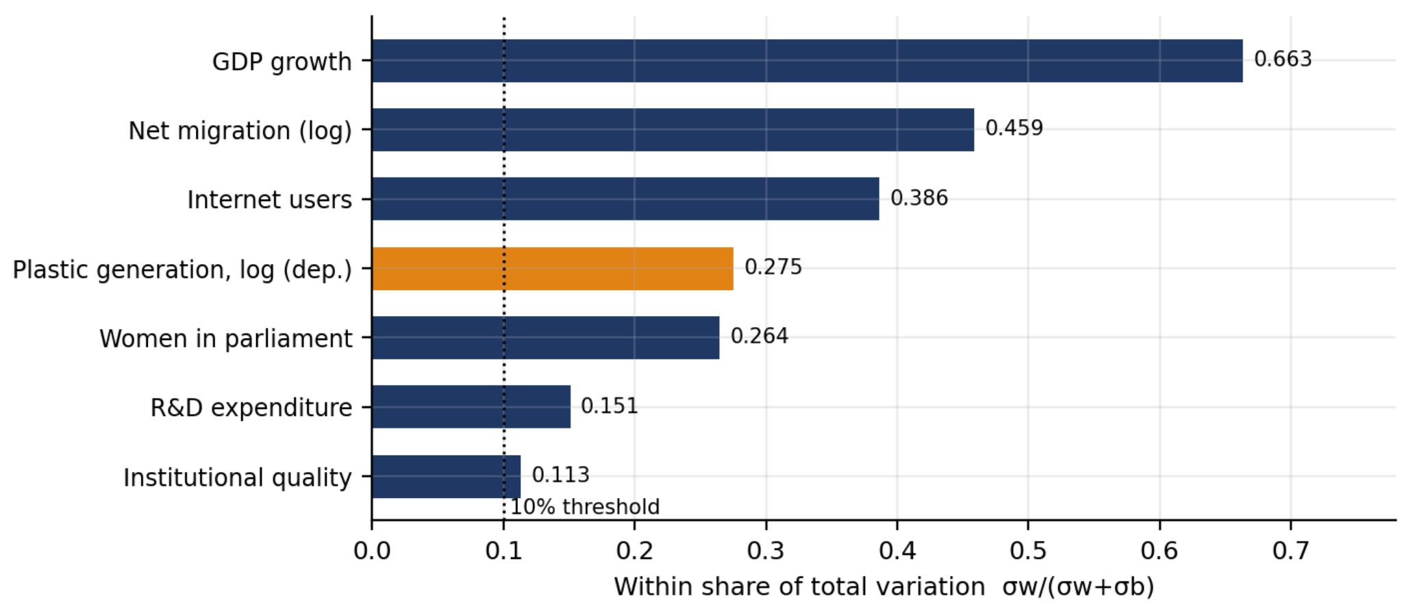
Figure 19.
Standardised coefficients across estimators, with 95% confidence intervals, governance block.
Figure 19.
Standardised coefficients across estimators, with 95% confidence intervals, governance block.
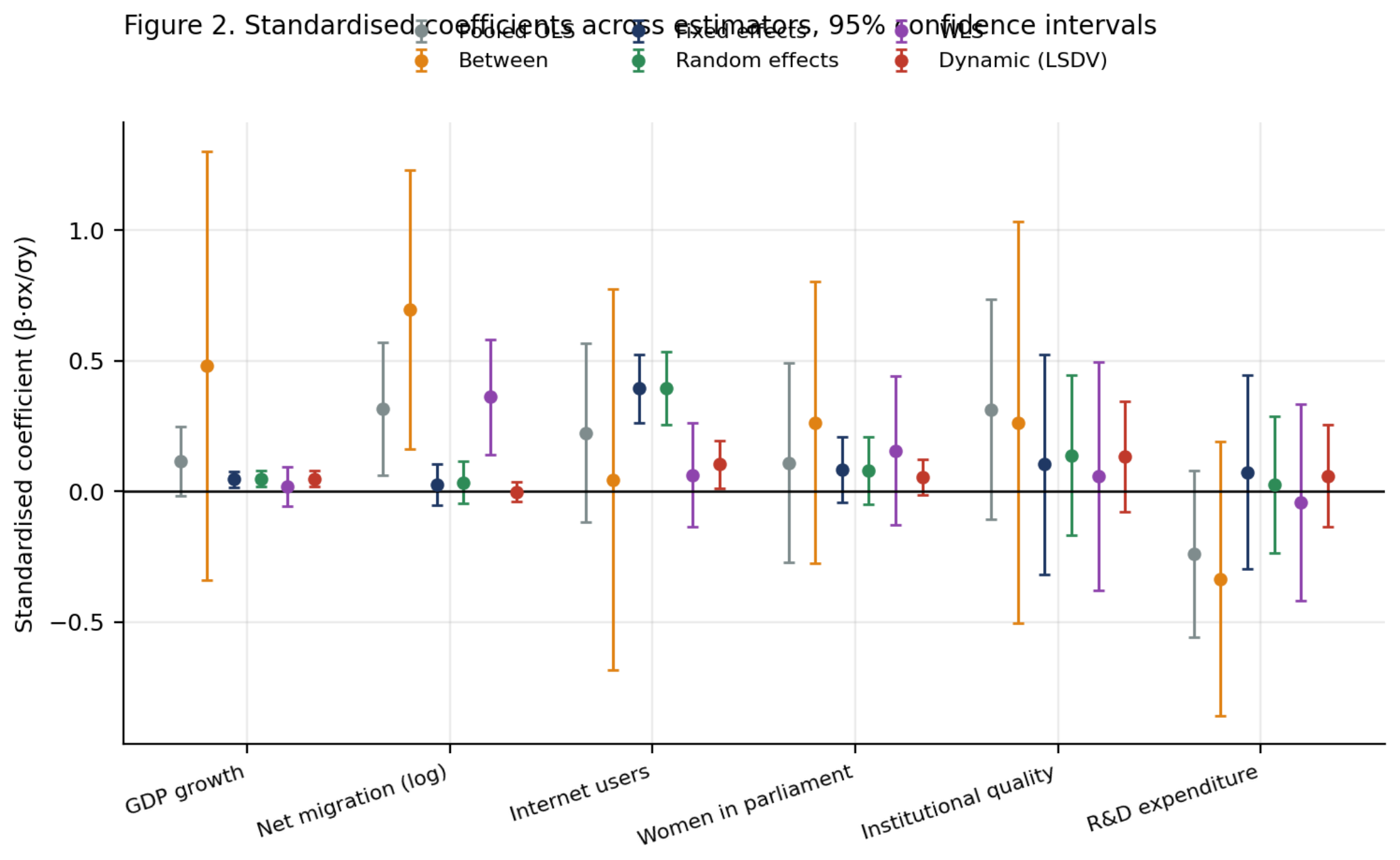
Figure 20.
The six governance indicators entered individually.
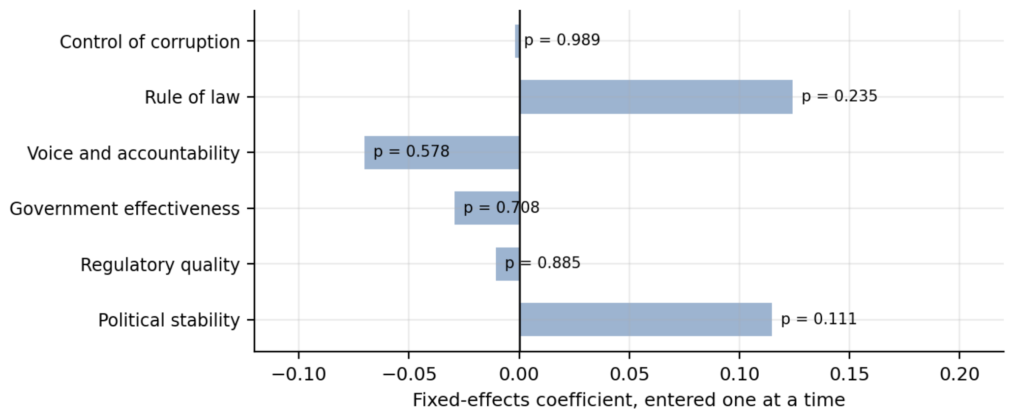
Figure 21.
Algorithm comparison by mean rank across eleven validity indices.
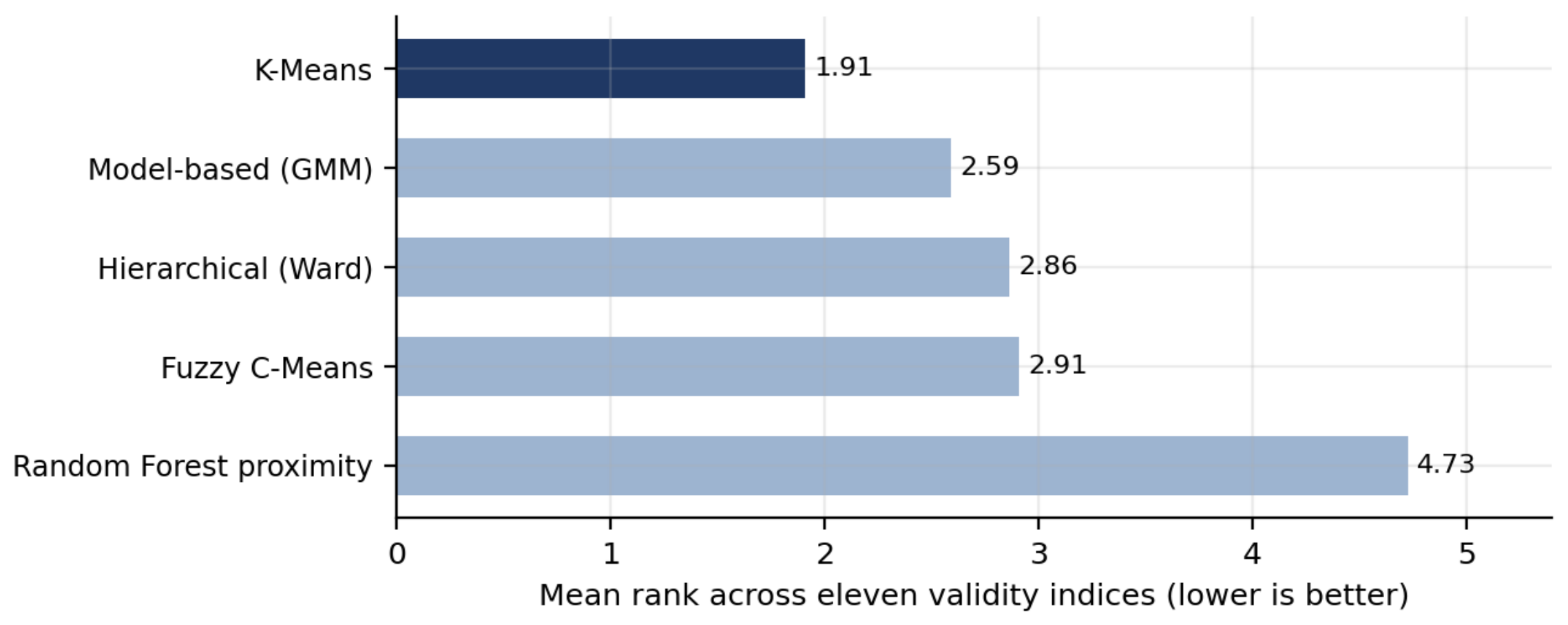
Figure 22.
Selection of the number of clusters, K-Means.
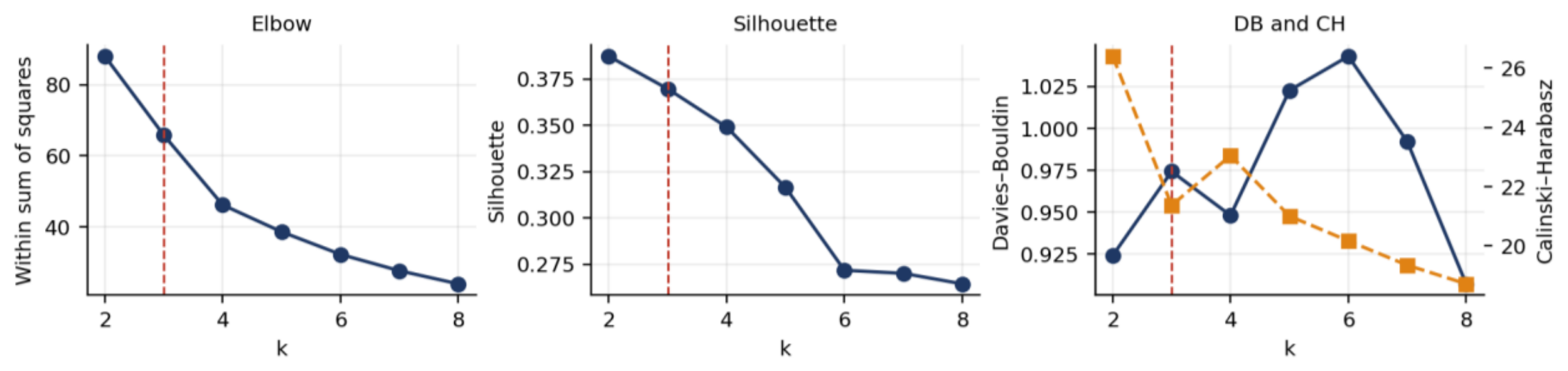
Figure 23.
Cluster membership in the space of the first two principal components.
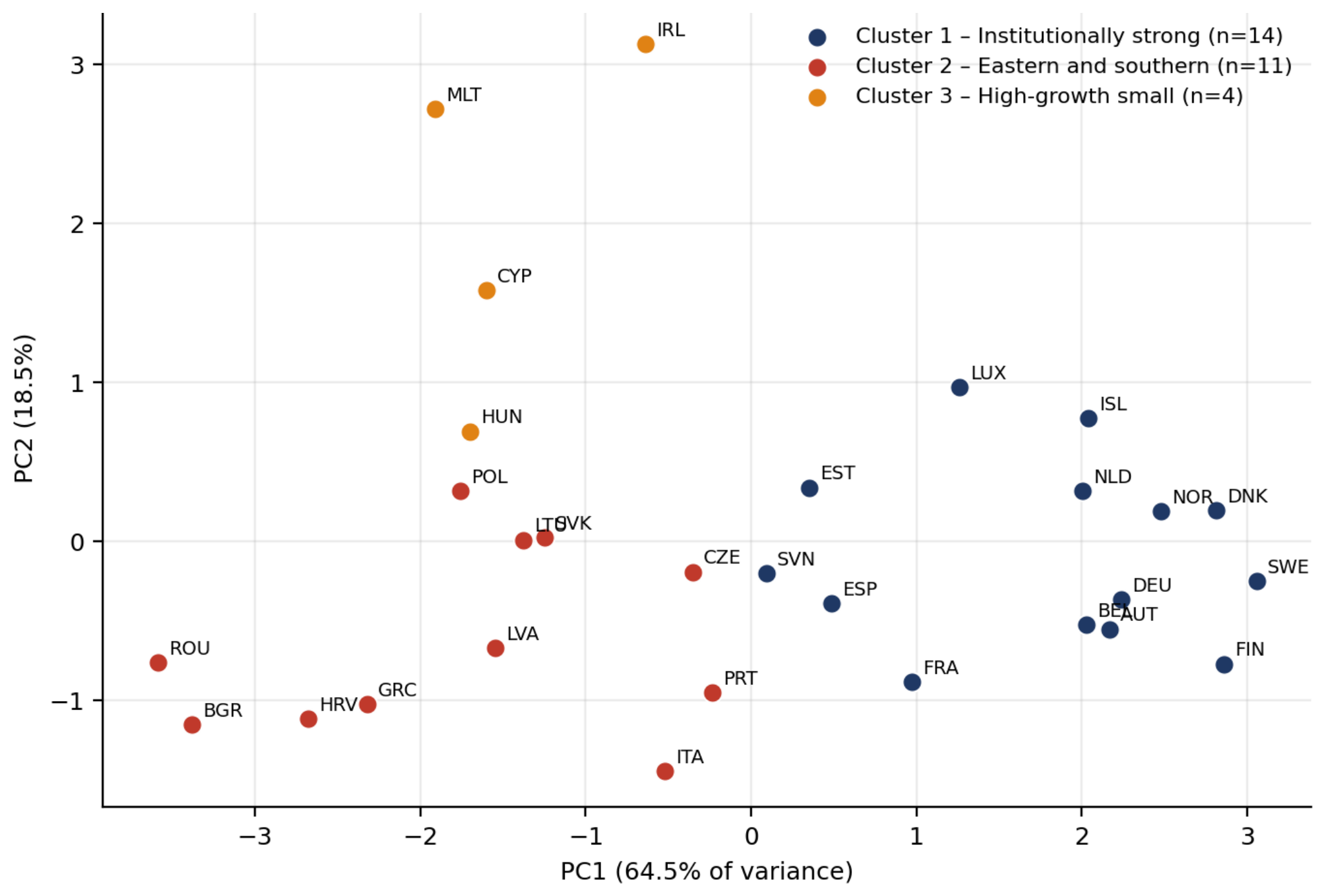
Figure 24.
External validation and cluster profiles.
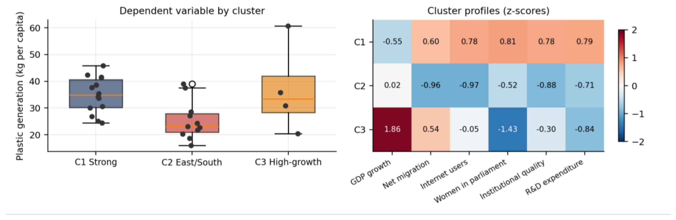
Figure 25.
Permutation importance across models and transformations.
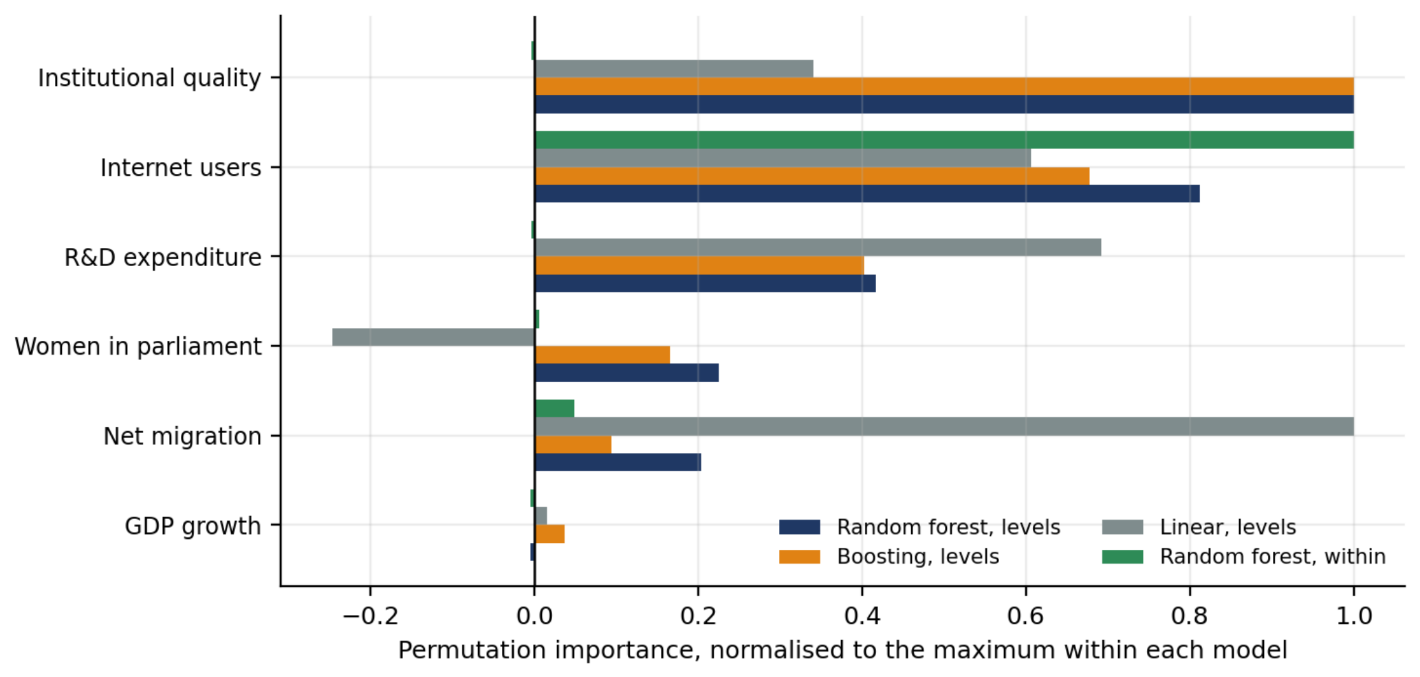
Figure 26.
Partial dependence in levels: where the linear model fails.
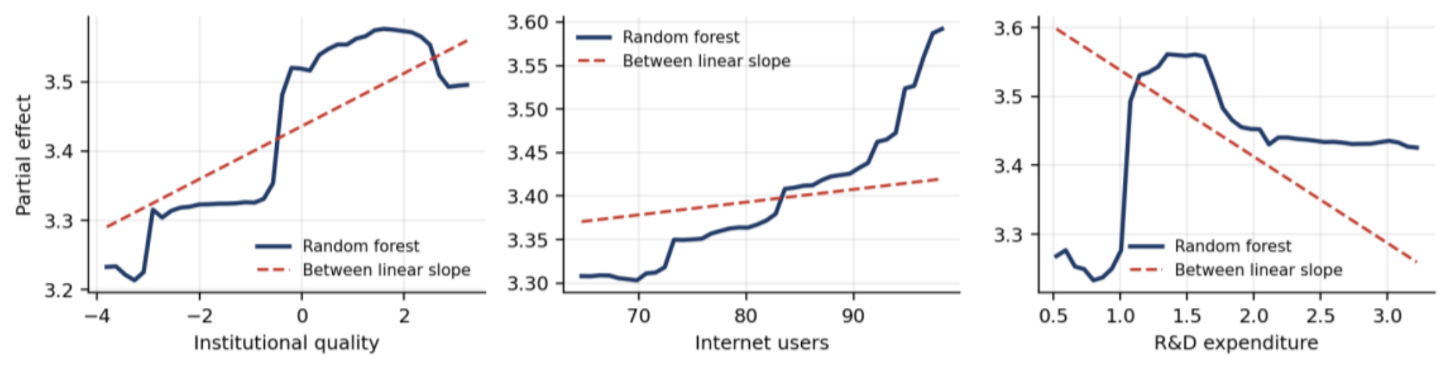
Table 1.
Environmental determinants of plastic packaging waste generation: comparison of six panel estimators.
Table 1.
Environmental determinants of plastic packaging waste generation: comparison of six panel estimators.
| Variable | Pooled OLS | Between | Fixed effects | Random effects | WLS | Dynamic (LSDV) |
|---|---|---|---|---|---|---|
| Lagged generation (log) | — | — | — | — | — | 0.6913*** |
| (0.0957) | ||||||
| Population density (log) | −0.0117 | 0.0125 | −0.8994 | −0.2257*** | 0.1097 | −0.2965 |
| (0.0817) | (0.1128) | (0.5517) | (0.0751) | (0.1164) | (0.1987) | |
| Energy intensity | −0.2077*** | −0.1915** | −0.4143*** | −0.3612*** | −0.2179*** | −0.1091 |
| (0.0478) | (0.0711) | (0.0652) | (0.0680) | (0.0612) | (0.0763) | |
| CO2 per capita | 0.0628*** | 0.0638*** | 0.0891*** | 0.0854*** | 0.0189 | 0.0224 |
| (0.0175) | (0.0205) | (0.0110) | (0.0109) | (0.0303) | (0.0150) | |
| Net energy imports | −0.0003 | −0.0004 | 0.0007*** | 0.0004* | −0.0007 | −0.0002 |
| (0.0003) | (0.0005) | (0.0003) | (0.0002) | (0.0004) | (0.0005) | |
| Forest area | 0.0014 | 0.0022 | −0.0564 | −0.0022 | 0.0055 | −0.0320** |
| (0.0043) | (0.0057) | (0.0497) | (0.0046) | (0.0055) | (0.0158) | |
| Protected areas | −0.0048 | −0.0053 | 0.0063** | 0.0034 | 0.0008 | 0.0011 |
| (0.0036) | (0.0055) | (0.0029) | (0.0025) | (0.0032) | (0.0009) | |
| Constant | 3.7555*** | 3.5612*** | 10.0718*** | 4.9857*** | 3.3261*** | 3.7476*** |
| (0.5143) | (0.6278) | (3.3576) | (0.3948) | (0.7876) | (1.0487) | |
| Observations | 243 | 28 | 243 | 243 | 243 | 215 |
| Countries | 28 | 28 | 28 | 28 | 28 | 28 |
| R2 | 0.455 | 0.465 | 0.451 | 0.413 | 0.380 | 0.652 |
Note. *** p<0.01, ** p<0.05, * p<0.10. WLS weighted by population. Between estimated on country means.
Table 2.
Specification and diagnostic tests, environmental panel.
| Test | Null hypothesis | Statistic | p-value |
|---|---|---|---|
| F test on individual effects | No country effects (pooling) | F(27, 209) = 51.50 | 0.000 |
| Breusch–Pagan LM | No random effects | χ2(1) = 65.32 | 0.000 |
| Mundlak Wald (robust Hausman) | Within equals between | χ2(6) = 21.25 | 0.002 |
| Pesaran CD | Cross-sectional independence | CD = 17.86 | 0.000 |
| Wooldridge AR(1) | No first-order serial correlation | ρ̂ = 0.333 | 0.000 |
| Breusch–Pagan | Homoskedasticity | χ2(6) = 30.61 | 0.000 |
Note. All tests reject their null. Pooling and random effects are rejected, so fixed effects is the specification interpreted. Errors are cross-sectionally dependent, serially correlated and heteroskedastic; clustering by country addresses the latter two. (35 words).
Table 4.
Comparison of six clustering algorithms on eleven validity indices, environmental block.
| Algorithm | R2 | AIC | BIC | Silhouette | Max. diameter | Min. separation | Pearson | Dunn | Entropy | Calinski–Harabasz | HHI |
|---|---|---|---|---|---|---|---|---|---|---|---|
| K-Means | 0.426 | 425.61 | 453.59 | 0.242 | 5.610 | 0.903 | 0.429 | 0.161 | 1.038 | 9.263 | 0.370 |
| Hierarchical (Ward) | 0.422 | 426.66 | 454.63 | 0.245 | 5.610 | 1.302 | 0.441 | 0.232 | 1.032 | 9.128 | 0.375 |
| Model-based (GMM) | 0.362 | 443.36 | 471.34 | 0.338 | 5.610 | 1.064 | 0.669 | 0.190 | 0.559 | 7.081 | 0.696 |
| Fuzzy C-Means | 0.417 | 428.27 | 456.24 | 0.226 | 5.610 | 0.903 | 0.403 | 0.161 | 1.061 | 8.922 | 0.357 |
| Random Forest proximity | 0.328 | 451.87 | 479.85 | 0.106 | 6.515 | 0.751 | 0.237 | 0.115 | 1.097 | 6.114 | 0.334 |
| Density-based (DBSCAN) | 0.911 | 99.27 | 117.93 | 0.420 | 2.857 | 1.302 | 0.059 | 0.456 | 0.580 | 12.078 | 0.609 |
Note. DBSCAN estimated with ε = 1.30 and a minimum of three points; it assigns 15 of 28 countries and labels the remaining 13 as noise.
Table 5.
Environmental cluster profiles in standardised units.
| Cluster | Pop. density (log) | Energy intensity | CO2 per capita | Net energy imports | Forest area | Protected areas | n |
|---|---|---|---|---|---|---|---|
| 1. Nordic-Baltic forested | −1.519 | 0.948 | 0.294 | −1.009 | 1.364 | −0.631 | 5 |
| 2. Continental carbon-intensive | 0.500 | 0.364 | 0.686 | 0.103 | 0.017 | 0.985 | 10 |
| 3. Mediterranean import-dependent | 0.200 | −0.644 | −0.641 | 0.309 | −0.538 | −0.515 | 13 |
Note. Ward linkage on standardised country means, 2014–2022. Analysis of variance across clusters is significant at the 1% level for five of the six indicators and at the 5% level for the sixth.
Table 6.
Predictive performance of six supervised learners in levels, environmental block.
| Algorithm | R2 | RMSE | MAE | MAPE (%) | Correlation | Median AE | Mean rank |
|---|---|---|---|---|---|---|---|
| Linear regression | 0.191 | 0.293 | 0.231 | 6.91 | 0.522 | 0.182 | 1.17 |
| K-nearest neighbours | −0.015 | 0.328 | 0.245 | 7.24 | 0.369 | 0.176 | 2.33 |
| Linear SVM | 0.102 | 0.309 | 0.249 | 7.49 | 0.521 | 0.202 | 2.67 |
| Boosting | −0.157 | 0.351 | 0.263 | 7.70 | 0.177 | 0.189 | 4.33 |
| Random forest | −0.068 | 0.337 | 0.267 | 7.90 | 0.235 | 0.205 | 4.50 |
| Decision tree | −0.453 | 0.393 | 0.306 | 9.07 | 0.112 | 0.231 | 6.00 |
Note. Levels, ten-fold grouped cross-validation by country, N = 243.
Table 7.
Permutation importance across models and transformations, environmental block.
| Variable | Linear, levels | Random forest, levels | Random forest, within | Boosting, within |
|---|---|---|---|---|
| Energy intensity | 0.0728 | 0.0418 | 0.0145 | 0.0150 |
| CO2 per capita | 0.0243 | −0.0010 | 0.0009 | 0.0010 |
| Net energy imports | 0.0115 | 0.0101 | −0.0002 | −0.0002 |
| Protected areas | 0.0067 | −0.0023 | −0.0000 | −0.0004 |
| Population density (log) | −0.0003 | 0.0030 | 0.0023 | 0.0033 |
| Forest area | −0.0005 | 0.0056 | −0.0002 | 0.0002 |
Note. Importance in units of mean squared error, averaged over ten held-out folds. Negative values indicate that permuting the variable improves prediction. Energy intensity ranks first in all four columns; density and forest area carry no predictive content.
Table 8.
Social determinants of plastic packaging waste generation: comparison of six panel estimators.
Table 8.
Social determinants of plastic packaging waste generation: comparison of six panel estimators.
| Variable | Pooled OLS | Between | Fixed effects | Random effects | WLS | Dynamic (LSDV) |
|---|---|---|---|---|---|---|
| Lagged generation (log) | — | — | — | — | — | 0.7053*** |
| (0.0727) | ||||||
| Population aged 65+ | −0.0111 | −0.0187 | 0.0446** | 0.0258** | −0.0154 | 0.0052 |
| (0.0216) | (0.0192) | (0.0198) | (0.0124) | (0.0172) | (0.0127) | |
| Fertility rate | 0.1041 | 0.1374 | −0.0696 | −0.0381 | −0.1643*** | 0.0180 |
| (0.2271) | (0.3222) | (0.1444) | (0.1416) | (0.0548) | (0.0707) | |
| Labour force participation | 0.0076 | 0.0052 | 0.0112 | 0.0159** | 0.0046 | 0.0038 |
| (0.0070) | (0.0101) | (0.0098) | (0.0074) | (0.0038) | (0.0038) | |
| Unemployment rate | −0.0352*** | −0.0356** | −0.0143* | −0.0179*** | −0.0347*** | −0.0045 |
| (0.0076) | (0.0166) | (0.0074) | (0.0064) | (0.0077) | (0.0040) | |
| Gini index | 0.0301*** | 0.0321** | −0.0034 | −0.0026 | 0.0320*** | −0.0039 |
| (0.0112) | (0.0151) | (0.0097) | (0.0076) | (0.0099) | (0.0039) | |
| Life expectancy | 0.0693*** | 0.0721*** | −0.0227** | 0.0010 | 0.0827*** | −0.0071 |
| (0.0138) | (0.0186) | (0.0092) | (0.0077) | (0.0122) | (0.0103) | |
| Constant | −3.3357** | −3.3506* | 3.8584*** | 1.9184** | −3.7342*** | 1.3329 |
| (1.3526) | (1.8309) | (1.0313) | (0.8303) | (0.8237) | (1.1109) | |
| Observations | 270 | 29 | 270 | 270 | 270 | 241 |
| Countries | 29 | 29 | 29 | 29 | 29 | 29 |
| R2 | 0.471 | 0.526 | 0.460 | 0.451 | 0.635 | 0.685 |
Note. Dependent variable: natural logarithm of plastic packaging waste generated per capita. Cluster-robust standard errors by country in parentheses. *** p<0.01, ** p<0.05, * p<0.10. WLS weighted by population; Between estimated on country means; Dynamic column estimated by least squares dummy variable. Sample: 29 countries, 2014–2023. Life expectancy and the Gini index reverse sign between the between and within estimators.
Table 9.
Specification and diagnostic tests, social panel.
| Test | Null hypothesis | Statistic | p-value |
|---|---|---|---|
| F test on individual effects | No country effects (pooling) | F(28, 235) = 56.95 | 0.000 |
| Breusch–Pagan LM | No random effects | χ2(1) = 74.39 | 0.000 |
| Mundlak Wald (robust Hausman) | Within equals between | χ2(6) = 33.91 | 0.000 |
| Pesaran CD | Cross-sectional independence | CD = −0.84 | 0.399 |
| Wooldridge AR(1) | No first-order serial correlation | ρ̂ = 0.657 | 0.000 |
| Breusch–Pagan | Homoskedasticity | χ2(6) = 20.48 | 0.002 |
Note. Pooling and random effects are rejected, so fixed effects is the specification interpreted. Cross-sectional independence is not rejected here, unlike in the environmental block; residuals remain serially correlated and heteroskedastic, both addressed by clustering.
Table 10.
Comparison of six clustering algorithms on eleven validity indices, social block.
| Algorithm | R2 | AIC | BIC | Silhouette | Max. diameter | Min. separation | Pearson | Dunn | Entropy | Calinski–Harabasz | HHI |
|---|---|---|---|---|---|---|---|---|---|---|---|
| K-Means | 0.430 | 437.91 | 466.63 | 0.256 | 4.793 | 1.636 | 0.542 | 0.341 | 0.912 | 9.816 | 0.463 |
| Hierarchical (Ward) | 0.404 | 445.77 | 474.48 | 0.270 | 5.827 | 1.636 | 0.579 | 0.281 | 0.780 | 8.809 | 0.562 |
| Model-based (GMM) | 0.331 | 465.92 | 494.63 | 0.162 | 6.225 | 1.208 | 0.403 | 0.194 | 0.833 | 6.424 | 0.524 |
| Fuzzy C-Means | 0.399 | 447.10 | 475.82 | 0.219 | 5.071 | 1.454 | 0.471 | 0.287 | 1.053 | 8.642 | 0.363 |
| Random Forest proximity | 0.306 | 472.16 | 500.88 | 0.104 | 5.415 | 1.353 | 0.265 | 0.250 | 1.031 | 5.739 | 0.375 |
| Density-based (DBSCAN) | 0.383 | 437.73 | 456.87 | 0.342 | 5.071 | 2.608 | 0.459 | 0.514 | 0.279 | 6.030 | 0.853 |
Note. DBSCAN estimated with ε = 2.15 and a minimum of two points; it assigns 25 of 29 countries to two groups and labels four as noise.
Table 11.
Social cluster profiles in standardised units.
| Cluster | Age 65+ | Fertility | Labour force part. | Unemployment | Gini | Life expectancy | n |
|---|---|---|---|---|---|---|---|
| 1. Eastern transition | 0.148 | 0.119 | −0.668 | −0.069 | 0.783 | −1.507 | 7 |
| 2. Southern high-unemployment | 1.092 | −1.344 | −0.788 | 1.828 | 1.017 | 0.762 | 4 |
| 3. Western and Nordic | −0.300 | 0.252 | 0.435 | −0.379 | −0.530 | 0.417 | 18 |
Note. K-Means on standardised country means, 2014–2023. Analysis of variance across clusters is significant at the 5% level or better for all six indicators.
Table 12.
Predictive performance of six supervised learners in levels, social block.
| Algorithm | R2 | RMSE | MAE | MAPE (%) | Correlation | Median AE | Mean rank |
|---|---|---|---|---|---|---|---|
| Linear SVM | 0.172 | 0.297 | 0.231 | 6.92 | 0.511 | 0.190 | 1.17 |
| Linear regression | 0.107 | 0.308 | 0.233 | 6.96 | 0.462 | 0.173 | 1.83 |
| K-nearest neighbours | 0.095 | 0.310 | 0.242 | 7.31 | 0.447 | 0.201 | 3.00 |
| Random forest | −0.224 | 0.361 | 0.279 | 8.39 | 0.304 | 0.226 | 4.00 |
| Boosting | −0.268 | 0.367 | 0.281 | 8.46 | 0.288 | 0.237 | 5.00 |
| Decision tree | −0.470 | 0.395 | 0.306 | 9.22 | 0.221 | 0.269 | 6.00 |
Note. Levels, ten-fold grouped cross-validation by country, N = 270.
Table 13.
Permutation importance across models and transformations, social block.
| Variable | Linear SVM, levels | Linear, levels | Linear SVM, within | Random forest, within |
|---|---|---|---|---|
| Life expectancy | 0.0669 | 0.0598 | 0.0002 | −0.0000 |
| Gini index | 0.0312 | 0.0248 | −0.0002 | −0.0001 |
| Unemployment rate | 0.0310 | 0.0311 | 0.0017 | 0.0014 |
| Labour force participation | 0.0017 | 0.0015 | 0.0006 | −0.0007 |
| Population aged 65+ | −0.0015 | −0.0033 | 0.0034 | 0.0069 |
| Fertility rate | −0.0051 | −0.0060 | −0.0002 | 0.0006 |
Note. Permutation importance in units of mean squared error, averaged over ten held-out folds.
Table 14.
Governance determinants of plastic packaging waste generation: comparison of six panel estimators.
Table 14.
Governance determinants of plastic packaging waste generation: comparison of six panel estimators.
| Variable | Pooled OLS | Between | Fixed effects | Random effects | WLS | Dynamic (LSDV) |
|---|---|---|---|---|---|---|
| Lagged generation (log) | — | — | — | — | — | 0.6533*** |
| (0.0702) | ||||||
| GDP growth | 0.0100* | 0.0418 | 0.0041*** | 0.0042*** | 0.0016 | 0.0042*** |
| (0.0058) | (0.0344) | (0.0013) | (0.0014) | (0.0033) | (0.0013) | |
| Net migration (log) | 0.0133** | 0.0292** | 0.0011 | 0.0014 | 0.0152*** | −0.0001 |
| (0.0054) | (0.0108) | (0.0017) | (0.0017) | (0.0047) | (0.0008) | |
| Internet users | 0.0072 | 0.0015 | 0.0127*** | 0.0128*** | 0.0020 | 0.0033** |
| (0.0056) | (0.0113) | (0.0021) | (0.0023) | (0.0033) | (0.0015) | |
| Women in parliament | 0.0035 | 0.0085 | 0.0027 | 0.0025 | 0.0050 | 0.0017 |
| (0.0062) | (0.0083) | (0.0020) | (0.0021) | (0.0046) | (0.0011) | |
| Institutional quality (PC1) | 0.0455 | 0.0382 | 0.0151 | 0.0200 | 0.0087 | 0.0192 |
| (0.0310) | (0.0537) | (0.0310) | (0.0226) | (0.0322) | (0.0155) | |
| R&D expenditure | −0.0894 | −0.1253 | 0.0278 | 0.0094 | −0.0160 | 0.0222 |
| (0.0608) | (0.0947) | (0.0703) | (0.0498) | (0.0716) | (0.0372) | |
| Constant | 2.7402*** | 2.9497*** | 2.1939*** | 2.2193*** | 3.0610*** | 0.8197*** |
| (0.4479) | (1.0454) | (0.1761) | (0.1907) | (0.3115) | (0.1280) | |
| Observations | 282 | 29 | 282 | 282 | 282 | 253 |
| Countries | 29 | 29 | 29 | 29 | 29 | 29 |
| R2 | 0.438 | 0.566 | 0.466 | 0.447 | 0.407 | 0.693 |
Note. Dependent variable: natural logarithm of plastic packaging waste generated per capita. Cluster-robust standard errors by country in parentheses. *** p<0.01, ** p<0.05, * p<0.10. WLS weighted by population; Between estimated on country means. Sample: 29 countries, 2014–2023. Institutional quality is the first principal component of the six Worldwide Governance Indicators.
Table 15.
Comparison of six clustering algorithms on eleven validity indices, governance block.
| Algorithm | R2 | AIC | BIC | Silhouette | Max. diameter | Min. separation | Pearson | Dunn | Entropy | Calinski–Harabasz | HHI |
|---|---|---|---|---|---|---|---|---|---|---|---|
| K-Means | 0.622 | 366.61 | 395.33 | 0.370 | 4.182 | 1.279 | 0.661 | 0.306 | 0.993 | 21.372 | 0.396 |
| Hierarchical (Ward) | 0.597 | 377.72 | 406.44 | 0.379 | 4.493 | 1.452 | 0.663 | 0.323 | 0.911 | 19.246 | 0.451 |
| Model-based (GMM) | 0.602 | 375.69 | 404.41 | 0.378 | 4.493 | 1.452 | 0.657 | 0.323 | 0.942 | 19.624 | 0.439 |
| Fuzzy C-Means | 0.614 | 370.30 | 399.02 | 0.309 | 5.054 | 1.264 | 0.583 | 0.250 | 1.059 | 20.650 | 0.358 |
| Random Forest proximity | 0.522 | 407.36 | 436.08 | 0.250 | 5.094 | 1.370 | 0.579 | 0.269 | 0.797 | 14.195 | 0.489 |
| Density-based (DBSCAN) | 0.937 | 69.57 | 107.86 | 0.441 | 1.999 | 1.631 | 0.353 | 0.816 | 1.213 | 33.438 | 0.344 |
Note. DBSCAN estimated with ε = 1.30 and a minimum of two points; it assigns 16 of 29 countries to four groups and labels thirteen as noise.
Table 16.
Governance cluster profiles in standardised units.
| Cluster | GDP growth | Net migration | Internet users | Women in parl. | Inst. quality | R&D | n |
|---|---|---|---|---|---|---|---|
| 1. Institutionally strong | −0.552 | 0.605 | 0.775 | 0.815 | 0.775 | 0.794 | 14 |
| 2. Eastern and southern | 0.024 | −0.965 | −0.967 | −0.518 | −0.877 | −0.706 | 11 |
| 3. High-growth small economies | 1.865 | 0.536 | −0.052 | −1.428 | −0.301 | −0.837 | 4 |
Note. K-Means on standardised country means, 2014–2023. Each entry is the cluster mean expressed as a distance from the sample mean in standard deviations. Analysis of variance is significant at the 0.01% level for all six indicators.
Table 17.
Predictive performance of six supervised learners in levels, governance block.
| Algorithm | R2 | RMSE | MAE | MAPE (%) | Correlation | Median AE | Mean rank |
|---|---|---|---|---|---|---|---|
| Random forest | 0.445 | 0.243 | 0.193 | 5.70 | 0.675 | 0.156 | 1.33 |
| Boosting | 0.439 | 0.244 | 0.195 | 5.74 | 0.678 | 0.170 | 2.00 |
| Decision tree | 0.261 | 0.280 | 0.206 | 6.02 | 0.586 | 0.151 | 3.17 |
| K-nearest neighbours | 0.310 | 0.271 | 0.216 | 6.34 | 0.602 | 0.175 | 3.50 |
| Linear regression | 0.130 | 0.304 | 0.237 | 7.01 | 0.453 | 0.193 | 5.00 |
| Linear SVM | 0.082 | 0.312 | 0.247 | 7.26 | 0.450 | 0.199 | 6.00 |
Note. Levels, ten-fold grouped cross-validation by country, N = 282.
Table 18.
Permutation importance across models and transformations, governance block.
| Variable | Random forest, levels | Boosting, levels | Linear, levels | Random forest, within |
|---|---|---|---|---|
| Institutional quality | 0.0241 | 0.0277 | 0.0065 | −0.0000 |
| Internet users | 0.0196 | 0.0188 | 0.0115 | 0.0106 |
| R&D expenditure | 0.0101 | 0.0111 | 0.0132 | −0.0000 |
| Women in parliament | 0.0054 | 0.0046 | −0.0047 | 0.0001 |
| Net migration (log) | 0.0049 | 0.0026 | 0.0190 | 0.0005 |
| GDP growth | −0.0001 | 0.0010 | 0.0003 | −0.0001 |
Note. Importance in units of mean squared error, averaged over ten held-out folds. Institutional quality ranks first in both flexible models yet is insignificant in every linear panel estimate, indicating a non-linear relationship.
Table 19.
Synthesis of findings across the three ESG pillars and the three methodological modules.
| Pillar | Panel econometrics | Machine learning clustering | Machine learning regression |
|---|---|---|---|
| E — Environment | The pillar operates through the metabolic intensity of production rather than through natural endowment. Energy and carbon intensity carry the result and survive every robustness check imposed, while land-based indicators are discarded not because they are insignificant but because they scarcely move within countries, so the within estimator has no information on which to identify them. The distinction matters: nominal significance here would have been an artefact of dividing a coefficient by a near-zero standard deviation. | The pillar fails the external test. Countries separate cleanly into recognisable environmental types, yet those types carry no information about how much plastic packaging they generate. The explanation is internal to the method: clustering weights all dimensions equally and groups by overall resemblance, so two partial effects of opposite sign on positively correlated indicators cancel within each type. Partial effects and typological similarity are distinct objects, and a strong result of the first kind does not imply one of the second. | The linear specification is vindicated. No algorithm capable of representing interactions or thresholds improves on ordinary least squares when predicting an unseen country, which is a stronger endorsement of functional form than any in-sample test because it is made out of sample. The learners independently discard the same two indicators that the variance decomposition rejected, so two unrelated criteria converge on the same exclusion. |
| S — Social | The pillar explains cross-country differences better than the environmental one, but its strongest association is also its least identified. Life expectancy reverses sign between the two dimensions, and the reversal is not noise: between countries it proxies the level of development, within a country over ten years it cannot, because it barely moves. The cyclical response to unemployment is the only association that holds its sign in both dimensions and is therefore the most defensible result of the pillar. | The pillar passes the external test, and this is the clearest contrast with the environmental block. Social configurations map onto packaging generation, though the contrast proves binary rather than threefold: the post-transition economies stand apart, while southern and north-western Europe are indistinguishable despite very different labour market and demographic profiles. Demographic contraction and labour slack do not translate into lower generation once development is comparable. | The linear form is adequate in both dimensions, an endorsement the environmental pillar did not obtain. More importantly, the learners recover two different variable hierarchies, one for the cross-section and one for the time dimension, and each reproduces the corresponding econometric column. An algorithm with no knowledge of panel econometrics finds life expectancy informative across countries and worthless within them, confirming the reversal by an independent route. |
| G — Governance | The pillar delivers its strongest results through channels that are not governance in the institutional sense. The growth cycle and the diffusion of online retail carry the explanation, the latter being the most robust association in the entire study. Institutional quality does not enter, and the null holds against the composite index and against every one of its components taken separately, which forecloses the objection that aggregation concealed a result. | The partition is technically the sharpest of the three, yet interpretatively the most constrained. Governance types do separate generation, but along the same boundary the social partition identified, and that boundary tracks the distribution of income. Cluster analysis on aggregate country indicators cannot distinguish a governance effect from a development effect when the two are nearly collinear, and here they are. | This is the only module in which flexibility wins, and the finding is specific rather than general: the linear form holds within countries and fails between them. Institutional quality, absent from every linear estimate, becomes the most important cross-sectional predictor once the functional form is unrestricted, and its partial dependence is flat below the median and rising above it. The panel result was correct about linear association and incomplete about the variable. |
Note. Each cell states what the method established for that pillar and how it should be read. Rows correspond to the three ESG pillars, columns to the three modules of Section 4 to 12.
Disclaimer/Publisher’s Note: The statements, opinions and data contained in all publications are solely those of the individual author(s) and contributor(s) and not of MDPI and/or the editor(s). MDPI and/or the editor(s) disclaim responsibility for any injury to people or property resulting from any ideas, methods, instructions or products referred to in the content. |
© 2026 by the authors. Licensee MDPI, Basel, Switzerland. This article is an open access article distributed under the terms and conditions of the Creative Commons Attribution (CC BY) license (http://creativecommons.org/licenses/by/4.0/).
Copyright: This open access article is published under a Creative Commons CC BY 4.0 license, which permit the free download, distribution, and reuse, provided that the author and preprint are cited in any reuse.