
Submitted:
29 August 2026
Posted:
31 August 2026
You are already at the latest version
Abstract
Santiago's Metro network is undergoing its largest expansion since 1975 through three new lines—L7, L8, and L9—announced in two waves (2017 and 2018) and opening on staggered timelines through 2033. This multi-cohort rollout is a setting where conventional two-way fixed-effects (TWFE) designs are known to misestimate treatment effects through negative-weighting bias, while static net-present-value rules ignore the option value of deferring irreversible construction under uncertainty. We address both using a hexagon-semester panel (2010S1–2025S2; N = 67,072) and a hedonic cross-section (N = 647,849) built from Chile's SII cadastre and F2890 registry, combining Callaway and Sant'Anna's group-time estimator with a linear-programming HonestDiD sensitivity analysis and a real-options investment-timing model calibrated on the panel's own empirical volatility and drift. We find a baseline pooled hedonic capitalization elasticity of +5.9% with respect to gravity accessibility, cohort-specific dynamics a pooled TWFE obscures, a non-monotonic anticipatory uplift across socioeconomic-disadvantage quintiles, and a capitalized land-value gain 1.8 times below the real-options investment trigger—indicating anticipated capitalization alone does not yet clear the option-adjusted threshold for accelerating construction, without speaking to the corridor's broader social return. The results caution against treating land value capture as a substitute, rather than a complement, to social cost–benefit justification for transit megaprojects.
Keywords:
transport infrastructure capitalization
; staggered difference-in-differences
; Callaway–Sant'Anna estimator
; HonestDiD
; real options
; land value capture
; distributive equity
; Metro de Santiago
1. Introduction
Rail transit investment is routinely justified on a claim that bundles two separate propositions: that a planned network's accessibility benefits will reach the areas that need them most, and that the housing market will recognize that value as the line advances toward completion. Transport-equity theory offers several normative standards for judging the first—utilitarian aggregate benefit, strict egalitarian access, a sufficientarian minimum threshold, and a Rawlsian prioritarian standard favoring society's least-advantaged members [1,2,3]—while accessibility's capitalization into price is, in Rosen's [4] hedonic framework, an empirical question about whether the market actually prices the amenity it is meant to benefit. Accessibility itself, following Hansen's [5] formulation and its later multidimensional elaborations [6], is the potential for interaction a network affords once travel impedance is properly accounted for, not mere physical proximity to a station—a distinction this paper's identification strategy takes seriously by working with accessibility-linked capitalization rather than simple distance-to-station proxies. This paper speaks primarily to the second proposition, and to an infrastructure-management decision this raises for any staggered, multi-year rollout: even once accessibility is shown to capitalize into price, deciding who benefits, when, and whether construction is currently justified requires an estimator robust to heterogeneous treatment timing and an investment-timing rule that prices the option to wait, not a static net-present-value comparison.
1.1. The Staggered Expansion of Metro de Santiago: L7, L8, and L9 in Context
Metro de Santiago has operated continuously since 1975 and today comprises seven lines, more than 136 stations, and approximately 140 km of track, carrying on the order of 2.3–2.5 million trips on an average weekday [7]. Between 2028 and 2033 the network is scheduled to add three further lines—L7, L8, and L9—representing 72 additional kilometers and 52 new stations: a single-decade expansion on a scale comparable to a substantial share of the network's entire history to date, and a policy-relevant test of the Metro's own role as a catalyst for public investment in the communes it reaches [8].
L7 was announced on 1 June 2017, during President Michelle Bachelet's public address to the nation. The line will run 26 km with 19 stations, connecting Renca in the northwest to Vitacura and Las Condes in the northeast through Cerro Navia, Quinta Normal, Santiago, Recoleta, and Providencia—eight communes in total, three of which (Renca, Cerro Navia, Vitacura) gain metro access for the first time [9]. Construction is underway, at roughly 40–42% physical progress as of mid-2026, with a reported construction cost of approximately US$2.53 billion and commercial opening planned for late 2028 [10].
L8 and L9 were announced jointly on 1 June 2018, during President Sebastián Piñera's first “Cuenta Pública.” L8 will run approximately 19 km with 14 stations, linking Providencia to Puente Alto through Ñuñoa, Macul, La Florida, and Peñalolén; its Environmental Impact Study received unanimous approval from Chile's Servicio de Evaluación Ambiental in 2026, at a reported construction cost of US$1.9 billion, with a phased opening across 2032–2033 [11,12]. L9 will run approximately 27 km with 19 stations along a corridor that historically lacked metro access—including La Pintana, San Ramón, La Granja, and Puente Alto—at a reported construction cost of US$2.733 billion, and has been under construction since August 2025, with a three-stage opening scheduled for 2030, 2032, and 2033 [13]. The original 2018 tender for both lines was declared void on 9 March 2020; the process was relaunched on 5 September 2021, with a formal call for basic-engineering tenders on 27 February 2022—verified against contemporaneous press coverage and Metro de Santiago's own corporate history (Section 2.2).
Figure 1.
Santiago Metro network: currently operating lines (L1–L6, solid markers) and projected lines (L7, L8, L9, and the under-construction L4A extension, open markers with official expected opening year), restricted to the Greater Santiago 34 (GS34) communal universe used throughout this paper's analysis.
Figure 1.
Santiago Metro network: currently operating lines (L1–L6, solid markers) and projected lines (L7, L8, L9, and the under-construction L4A extension, open markers with official expected opening year), restricted to the Greater Santiago 34 (GS34) communal universe used throughout this paper's analysis.
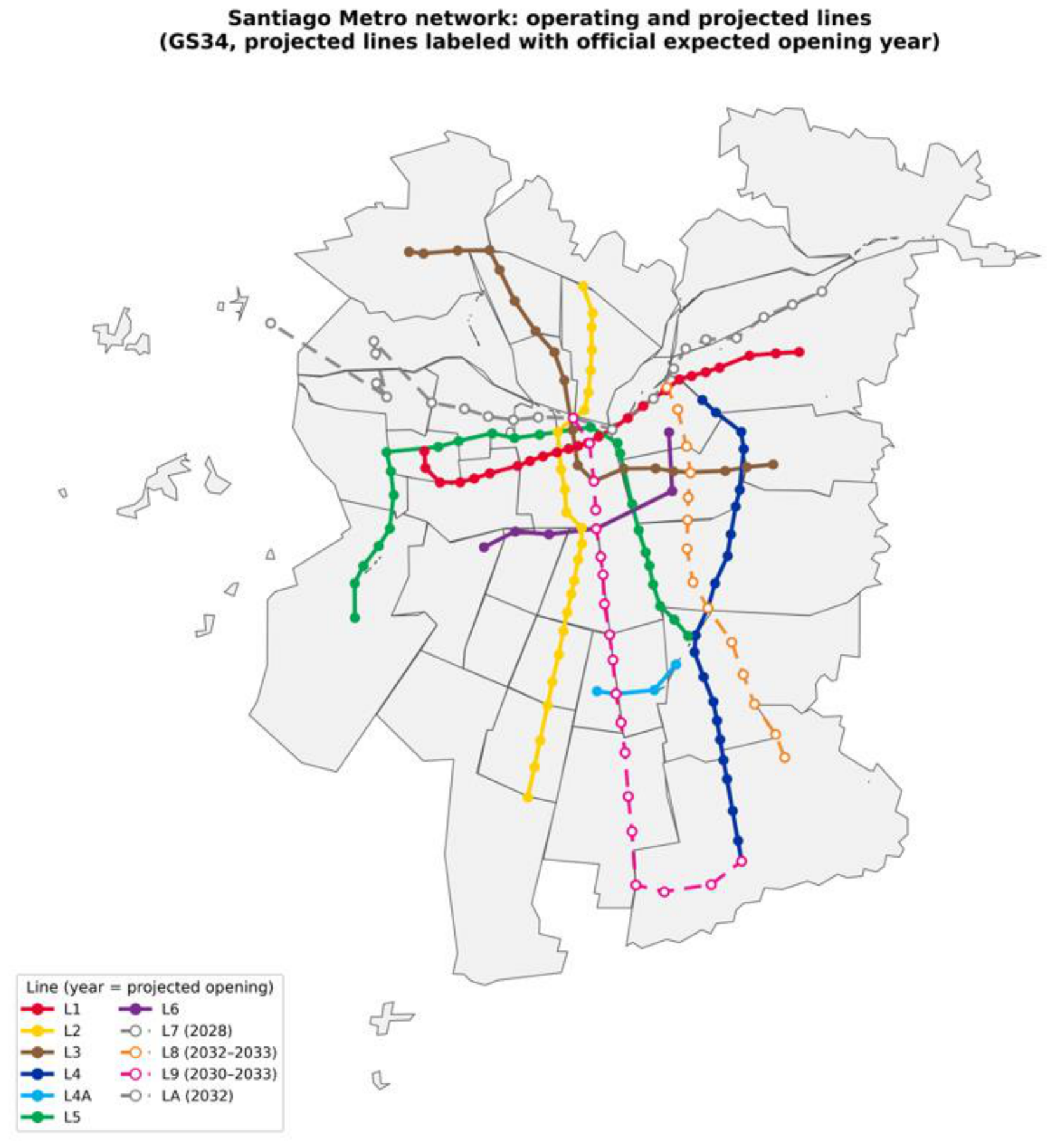
This sequence—two distinct announcement cohorts (2017S2 and 2018S1), a later administrative milestone (2022S1) that could plausibly serve as an alternative treatment date, and completion dates spread across nearly a decade—is exactly the setting in which the choice of difference-in-differences estimator is not a technical footnote but a substantive determinant of the paper's conclusions.
1.2. Literature Review: Global and Chilean Evidence
The theoretical foundation for reading transport-accessibility gains off residential prices is Rosen’s [4] hedonic price model, under which location-specific amenities—including travel-time savings—are implicitly priced through housing markets. Empirical applications consistently find anticipation, not only realized service, drives price responses: Chen et al.’s [18] analysis of Sydney’s Northwest Metro separately estimates an announcement stage (2008–2012) and construction stage (2013–2019), finding expectation effects accrued before the 2019 opening, with price premiums peaking one to two years before commercial operation. A quasi-experimental strand isolates causal effects directly: Gibbons and Machin’s [19] study of London’s Jubilee Line Extension and Docklands Light Railway found house-price increases attributable to the transport innovation itself, net of secular appreciation—an identification strategy this paper’s cohort-robust design (Section 2.5) extends to a multi-cohort, staggered-rollout setting.
Chile offers a deep applied literature here, since Metro de Santiago has expanded in discrete, dated increments since 1975. Agostini and Palmucci [20] find average apartment-price increases of 3.3–4.4% at Line 4's construction announcement and a further 4.5–5.7% once station locations were disclosed—evidence, over a decade before this design, that anticipation rather than realized service is the first-order channel. Aguirre Núñez et al. [21] corroborate this pattern on Line 3's later stations ahead of its 2019 opening. López-Morales et al. [22] extend the inquiry to distributive consequence, showing via a rent-gap framework that Metro investment in Greater Santiago (2008–2011) enlarged developers' captured ground rent by 25.6%—precisely the mechanism this paper's land-value-capture scenarios are designed to redirect. A later re-estimation, López-Morales et al. [23], finds Metro proximity raises land-seller capitalization by roughly 5% and apartment prices by roughly 9% while lowering the land-cost-to-price ratio, with capitalization differing systematically between older, affluent corridors and newer, less affluent ones. This paper's own +5.9% hedonic elasticity sits within this range, and its L8/L9 distributive analysis—concentrated in historically underserved La Pintana, San Ramón, and La Granja—engages directly with who ultimately captures the gain.
Meta-analyses caution against treating a station-distance coefficient as a transport-system constant: rail-station capitalization effects differ systematically by property type, technology, distance band, and context [24], with substantial heterogeneity from project maturity, land use, and empirical design [25]—a conclusion Higgins and Kanaroglou’s [26] review of over 130 land-value-uplift analyses across 60 North American studies confirms on a much larger evidence base, attributing part of the heterogeneity to reliance on station proximity rather than network-based accessibility. These findings motivate this study’s two choices: measuring network accessibility rather than Euclidean proximity, and separating announcement/construction from realized operation, since expected accessibility can capitalize before service begins even though sign and timing vary across projects [18,27]. The estimated +5.9% elasticity here should be read as a conditional association in Santiago’s current network, not a universal, transferable premium.
1.3. From TWFE to Heterogeneity-Robust DiD
The workhorse two-way fixed-effects (TWFE) regression is unbiased only when treatment timing is common across units or treatment effects are homogeneous across cohorts and time. Neither holds here: L7 and the L8/L9 pair are announced a year apart, occupy different catchments, and move construction activity and prices in different directions following announcement. This motivates the cohort-robust solution reviewed below [13,14,15,16,17,18].
A large recent econometric literature has re-examined canonical TWFE difference-in-differences once treatment timing varies across units—precisely what L7's 2017 and L8/L9's 2018 announcements create here. Goodman-Bacon [28] decomposes the TWFE estimator into a weighted average of every pairwise 2×2 comparison, showing that comparisons where an earlier-treated cohort controls for a later-treated one can carry negative weight, biasing the aggregate estimate in a direction that depends on treatment-effect dynamics rather than any modeling choice. Sun and Abraham [29] and de Chaisemartin and D'Haultfœuille [30] formalize the same concern for event studies and propose heterogeneity-robust alternatives. Callaway and Sant'Anna [16], whose ATT(g,t) this paper adopts as its primary estimator, aggregate cohort-specific 2×2 comparisons—each treated cohort against a not-yet- or never-treated group—without ever comparing treated cohorts to each other. Baker et al. [31] synthesize this literature into a practitioner's guide; Butts [32] extends the identification problem to this paper's spatial design specifically: when treatment effects spill over geographic boundaries, a control group's outcomes can be contaminated by proximity to treatment unless the control pool excludes spillover-exposed units—as this paper does by holding out communes hosting Line 3 or Line 6 stations.
Even a heterogeneity-robust estimator is only as credible as its identifying assumption—parallel trends absent treatment—which is untestable post-treatment. Rambachan and Roth [17] formalize how far this assumption can be relaxed before an effect’s sign is no longer identified, under two restrictions: bounded smoothness in the trend break (Δˢᴰ) and a magnitude bound relative to the largest pre-period deviation (Δᴿᴹ). Rather than a heuristic approximation, common in applied work, this paper implements its own linear-programming characterization directly (Section 2.6), reporting the breakdown value—the smallest violation at which the identified set first includes zero—for each headline outcome.
1.4. Real Options and Urban Development
A parallel identification problem arises on the investment side: the standard capital-budgeting rule (build once V ≥ I) holds only when investment is reversible or must be undertaken immediately—neither true for a metro line, whose construction is sunk while the state retains the option to delay. The real-options literature reviewed below [14,15] is applied to L8/L9’s timing decision.
A parallel tradition treats infrastructure and land-development decisions as options on an irreversible investment under uncertainty. McDonald and Siegel [15] derive the closed-form optimal investment trigger for a project whose value follows geometric Brownian motion: invest once value reaches a threshold V* strictly above construction cost I, with the option premium V*/I increasing in volatility and in the dividend foregone by waiting. Dixit and Pindyck [14] generalize this into the modern real-options framework, since applied extensively to urban land development, where a developer holds an implicit option to defer construction pending resolution of zoning, regulatory, or demand uncertainty.
Applying this to L8/L9's construction-timing question: the capitalized land-value gain is itself uncertain—this paper estimates its volatility empirically from the pipeline's own price data (Section 2.7)—and construction cannot be reversed. Under both conditions, the option value of waiting is strictly positive, and a policymaker evaluating “build now” purely against a static V ≥ I break-even will systematically under-value that option. This analysis is, to the author’s knowledge, among the first to apply this framework directly to a Latin American metro-expansion timing decision, using empirically estimated drift and volatility from the same panel used for the paper’s causal estimates, against L8 and L9’s real, publicly reported construction costs rather than a stylized project value.
1.5. Land Value Capture and Affordability
The connection between transit-induced land-value gains and public finance has generated a distinct land-value-capture (LVC) literature. LVC instruments include betterment contributions, special assessments, tax-increment mechanisms, joint development, development charges, and negotiated exactions. Their shared premise is that a portion of the increment associated with publicly provided accessibility may be returned to support infrastructure or related public purposes [33]. Yet the existence of capitalization is not by itself evidence that an instrument is fiscally feasible, legally authorized, administratively implementable, or distributionally neutral. Revenue depends on the tax base, timing of assessment, exemptions, market response, institutional capacity, and the allocation of risk between the public sector and private landowners [33,34].
This distinction is central in Santiago, where accessibility improvements may be capitalized in both owner-occupied values and rents, but the affected households need not be the landowners who receive the gain. The Santiago rent-gap evidence documents how infrastructure and planning can expand potential ground rents and create redevelopment pressure [22].
This tension between capitalization and displacement is not specific to Santiago. Zuk et al.'s [35] review of the North American transit-gentrification literature concludes that public transport investment is a documented, though not universal, trigger for neighborhood change, with outcomes depending heavily on pre-existing housing-market tightness and the presence or absence of protective policy; Fernando et al.'s [36] multi-indicator analysis of Manchester's Metrolink tram network similarly finds gentrification-like change concentrated in areas with sustained light-rail exposure, with mixed evidence on whether already-disinvested communities are more or less susceptible. Santiago's own socio-spatial history sharpens why this matters for the corridor evaluated here: Sabatini et al. [37] document that Chilean residential segregation has been shifting toward a larger geographic scale and increasing malignancy since land-market liberalization, and Figueroa Martínez et al. [38] show that social-housing policy has systematically located lower-income households in areas with the weakest public-transport connectivity in the city, a pattern this paper's L9-corridor high-risk hexagons (Section 3.10) sit squarely within. Pereira et al. [39] show empirically for Rio de Janeiro that an explicit equity rationale for a transit project does not by itself guarantee its largest accessibility gains reach the least-advantaged (Section 4.2 returns to this precedent); this paper treats the quintile-level and high-risk-hexagon evidence in Section 3 as the more informative test of L8/L9's distributive content than the presence of capitalization alone.
Therefore, the policy scenarios in this paper are deliberately interpreted as incidence-aware simulations of retained capitalization, rather than as forecasts of collectible revenue. A uniform capture rate can reduce a modeled premium proportionally while leaving its spatial distribution largely unchanged; a targeted affordability instrument can alter that distribution, but requires an explicit delivery mechanism—such as inclusionary requirements, social-rental protection, acquisition of land for affordable housing, or a legally specified betterment contribution—to be policy-operational. This framing places the paper's Scenario C in the LVC literature without overstating what a capitalization model alone can establish [33,34].
1.6. Contributions of This Study
This paper makes four contributions. First, it applies Callaway and Sant'Anna's [16] cohort-robust estimator, alongside a full linear-programming characterization of Rambachan and Roth's [17] HonestDiD identified set—rather than the heuristic approximation common in applied work—to a multi-cohort transit-capitalization design spanning 2,096 hexagons and 32 semesters, among the largest panels assembled for a Latin American transit system. Second, it documents that pooled TWFE and cohort-specific CS-DiD estimates for the same outcomes move in different, at times opposite, directions—an empirical demonstration, not a simulated illustration, of the practical consequences of staggered-treatment heterogeneity and cross-cohort comparisons that the recent econometric literature warns against. Third, it extends the equity question beyond a single triple-difference coefficient by comparing anticipatory price uplift across IST-2024 disadvantage quintiles and isolating hexagons where a large anticipated gain coincides with high disadvantage, revealing a pattern that departs from a simple, monotonic gentrification narrative. Fourth, it embeds a real-options investment-timing model—calibrated on the pipeline's own empirical drift and volatility not assumed parameters—directly into the policy conversation about L8/L9's construction timing and land value capture as a funding instrument, a question the capitalization literature typically leaves to a separate cost–benefit exercise. The quintile-level and high-risk-hexagon evidence developed in Section 3 speaks directly to whether disadvantaged residents capture a disproportionate, a proportionate, or a diminished share of the anticipated price gain—a distributive reading Section 4.2 returns to against the transport-equity literature’s prioritarian standard [1,2].
2. Materials and Methods
2.1. Data Sources
The empirical design draws on eight linked data sources (Table 1), consumed throughout the pipeline in Section 2.2. The panel window (2010S1–2025S2, 32 semesters) is set by the event-study design’s identification requirements, not a data ceiling: both the SII’s cadastral series and the F2890 transaction registry [40] carry genuine historical depth, and starting in 2010 gives a multi-year pre-announcement baseline for every cohort while remaining inside the modern, Unidad de Fomento (UF)-indexed real-estate regime. All variables are assembled at H3 resolution-8 hexagon–semester level (2,096 hexagons after estimation-sample restrictions), following the administrative microdata architecture validated in the author’s prior single-event airport-announcement design [41], extended here to a multi-line, multi-cohort rail-transit setting.
Population and the IST-2024 components are drawn from the 2024 Census cartography and published statistical tables, allocated to H3 hexagons dasymetrically—in proportion to residential floorspace rather than uniformly over area [42], since a block's geometric centroid is a poor proxy for where residents actually live when the block is large or irregular relative to the hexagon grid [43]. The resulting IST-2024 index is a weighted composite of z-scored block shares (overcrowding, unemployment, low schooling, tenure precarity, and related dimensions) oriented so lower values denote greater disadvantage, consistent with every downstream quintile, threshold, and high-risk classification in this paper (Section 3.9, Section 3.10 and Section 3.11). Its four declared dimensions—education, materiality, overcrowding, and employment—are equally weighted at 0.25 each. As an internal consistency check, the Pearson correlation between this index and its own first principal component is +0.783—below the 0.90 threshold for treating the two as interchangeable, disclosed here as an unresolved property of the weighting scheme. These four dimensions are structural, slowly-evolving neighborhood characteristics at the hexagon scale rather than fast-moving attributes, which mitigates, without eliminating, the pre-treatment timing concern Section 4.4 discloses for the panel-identified DDD.
2.2. Multi-Level Treatment Design and Cohorts
Unlike a single-announcement design, each of the three lines carries its own verified announcement date (Table 2), assigning per-line, per-cohort exposure rather than one binary indicator, established against contemporaneous press coverage and Metro de Santiago's own corporate history rather than a single administrative field.
The first public announcement is the primary treatment date used in the main specification (Section 2.4 and Section 2.5); the later re-tender milestone is carried as an explicit alternative for the robustness check reported in Section 3. Each hexagon is assigned one of four mutually exclusive roles (Table 3), adapted from a single-point-radius design to a rail-transit catchment.
The L3/L6 exclusion is not incidental: the panel window is wide enough to also span Line 3's and Line 6's own construction and opening, and a commune hosting either is held out of the never-treated pool for the full panel span rather than treated as a clean control—a “never-treated” group is only informative if it is genuinely untreated by any metro-proximity event, not just by L7/L8/L9 [32].
Spillovers to nearby, not-directly-treated hexagons are modeled using the hybrid spatial weight w_ij, a convex combination of a geographic and an economic-gravitational weight:
with a row-standardized k-nearest-neighbor geographic weight and d1/2 the distance at which economic connectivity halves (5 km, a stated intra-urban commuting-shed assumption, cross-checked in Section 3 against a decay parameter derived from the accessibility engine's own calibrated impedance).
2.3. Accessibility Engine and Gravity Decay Calibration
The gravity-based accessibility index Agrav used in the hedonic specification (Section 3) and in the spillover weight above follows Hansen’s [5] gravity formulation:
Aigrav = ΣjOj·exp(−β·cij)
Here, Agrav is computed over the street network, elevation nodes, and Metro station/line registries (Table 1). Door-to-door cost cij combines walking access/egress time, boarding wait, and in-vehicle travel time; walking time is slope-adjusted via Tobler's [44] hiking function, v(S) = 6·exp(−3.5·|S + 0.05|) km/h, since much of the GS34 footprint—particularly the eastern communes examined in Section 3.10—departs materially from level terrain.
The decay parameter β is calibrated against the observed mean public-transport trip time in the Encuesta Origen y Destino Santiago 2012 (Table 1), not assumed a priori: a route-choice logsum scale of μ = 0.0792 min⁻¹, targeting a half-life anchor of 58.53 min, yields β = 0.0118 min⁻¹. Since this target is time-decay while Equation (1)'s spillover weight is distance-based, the two are reconciled via the network's disclosed commercial speed (35 km/h): the resulting distance-decay, φecon = 0.0203 km−1 (half-life 34.1 km) is reported alongside the stated d1/2 = 5 km assumption as a robustness check (Table 11), treated as bounding cases rather than a single preferred value, since Section 3.6 finds the direct-effect estimate insensitive to the choice.
2.4. Baseline Two-Way Fixed-Effects Specification
The baseline specification, estimated separately for each outcome, is:
with hexagon fixed effects αi, semester fixed effects λt, and standard errors clustered by hexagon. With more than one treatment cohort, the single coefficient βdirect is a variance-weighted average that can be contaminated by the “forbidden comparisons” discussed in Section 1.2 [28]—which is why the cohort-robust estimator of Section 2.5 is the primary specification, and the TWFE coefficient above is reported only for comparability with earlier applied work.
Section 3.8’s equity triple-difference augments Equation (3) with a socioeconomic-disadvantage interaction, isolating whether treated hexagons in disadvantaged neighborhoods capitalize differently from the treated average:
where LowISTi is a hexagon-level indicator (Section 3.8 defines the specific threshold used) and controls reproduces Equation (3)’s did_comuna, spillover, and COVID terms unchanged; βDDD is the coefficient of interest, identifying the differential capitalization slope for disadvantaged hexagons net of both the average treatment effect and the average disadvantage-post trend.
2.5. The Callaway and Sant'Anna Estimator
With two genuine treatment cohorts—g = 2017S2 (L7) and g = 2018S1 (L8/L9)—against a never-treated control group, the group-time average treatment effect [16] is defined, for each cohort g and period t, as:
estimated as a manual, cohort-by-cohort 2×2 comparison—each treated cohort against the never-treated group—executed directly rather than delegated to a third-party staggered-DiD package, so that this paper's own validation suite (Section 2.6) is built against exactly the table it estimates. Estimates are aggregated into an event-study representation:
A companion equity triple-difference augments the same panel with an interaction between treatment, the post period, and IST-2024 disadvantage (LowIST), isolating whether treated hexagons in disadvantaged neighborhoods capitalize more or less than the treated average—reported in Section 3 alongside the ATT(g,t) results above.
2.6. HonestDiD Sensitivity Analysis
Every ATT(g,t) estimate is reported together with a formal sensitivity analysis [17] quantifying how large a parallel-trends violation would have to be to overturn its sign, implemented as the paper's own linear-programming identified-set characterization rather than a heuristic approximation. Under the smoothness restriction, the space of admissible post-treatment trend violations is:
and the identified set for θ̂_l (the equal-weighted average post-treatment effect used throughout this paper), with pre-period biases pinned to their observed values, is:
found by linear programming (its two extreme points) rather than a closed-form heuristic. Under the relative-magnitudes restriction, the identified set has a closed form once the largest pre-period first difference is computed:
Θl(M) = {l′δpost : δ ∈ ΔSD(M), δpre = βpre}
For each restriction, the breakdown value—the smallest violation (M* or M̄*) at which the identified set first includes zero—is reported alongside the point estimate in Section 3, directly answering how much of a parallel-trends violation it would take to overturn each result. This is the paper's identified-set characterization, not the full moment-inequality confidence-set inference, which would additionally require a conditional/hybrid test inversion beyond the present scope.
2.7. Real-Options Investment-Timing Model
A static net-present-value rule (“build if V ≥ I”) ignores two features the data demonstrate directly: the capitalized land-value gain V is uncertain, and the decision to build is irreversible but deferrable. Under both conditions the option to wait has positive value, and the correct investment trigger is higher than the naive V = I break-even [14,15]. As a standard valuation benchmark rather than a literal claim about the corridor’s true stochastic process, the capitalized value of building now, V, is assumed to follow a geometric Brownian motion:
Under the geometric Brownian motion of Equation (10), the value of the option to invest solves the standard perpetual-option ordinary differential equation, whose positive root β1 is:
Once β1 is known, the closed-form optimal investment trigger V* follows directly:
where I is construction cost, r the discount rate, and δ the opportunity cost of not yet having the accessibility gain in place (δ = r − α). Investing is optimal once V ≥ V*; V*/I is the option-value premium over the naive NPV = 0 rule, strictly increasing in σ. Every parameter is sourced, not assumed: σ and α come from this pipeline's own panel; r is Chile's Tasa Social de Descuento, appropriate here since the exercise adopts the public planner's perspective, not a private developer's cost of capital; I is L8/L9's combined, publicly reported construction cost, converted to UF at the Banco Central's published rate.
V prices the anticipated uplift across the L8/L9 catchment's full residential stock: median transacted price times anticipated uplift, scaled by each hexagon's household count and summed across the catchment, where uplift translates an accessibility gain (ΔA, log-points) into a price premium via the hedonic elasticity re-estimated from this pipeline's own data (Section 3):
where Agrav is the gravity-based accessibility index of Hansen [5] computed over the operative network scenario.
Section 3.11’s three land-value-capture scenarios apply a single mechanism—a capture rate ρ on the anticipated uplift, with an affordability lock capping high-risk hexagons’ retained uplift at κ—formalized once here rather than three times:
where 1{h∈HighRisk} is an indicator equal to 1 for the compound-risk hexagons Section 3.10 identifies and 0 otherwise, and the lock is switched off entirely (κ→∞, the indicator term vanishes) for the scenarios that do not apply it. Scenario A sets ρ=0; Scenario B sets ρ=0.30 with no lock; Scenario C sets ρ=0.20 with κ=0.08 applied only to high-risk hexagons.
Section 3 reports V, V*, the resulting invest/wait decision, and its sensitivity to the volatility parameter σ.
A generative AI tool (Claude, Anthropic) was used during pipeline development to audit intermediate outputs against exported datasets, help debug estimation code, and assist in drafting; it was not used to generate data, execute analyses unsupervised, or make inferential judgments, and all reported figures were verified by the authors against the pipeline’s own outputs.
3. Results
3.1. Current-Network Capitalization: Cross-Sectional Hedonic Evidence
Of 1,162,244 F2890 transactions in the panel window, 665,033 (57.2%) match to a residential property with structural attributes; 658,727 of these further match to the accessibility and IST-2024 layers via H3, yielding an estimation sample of 647,849 transactions after residual cleaning. Table 4 reports the hedonic specification of Section 2 (the log-price equation on log-gravity accessibility, floor area, age, IST-2024, and commune fixed effects) under three inference approaches.
The commune-clustered specification is primary given the residual spatial autocorrelation the same accessibility layer shows via LISA (Section 3.7); heteroskedasticity-robust-only SE would understate uncertainty under spatial dependence.
The point estimate is identical between pooled HC1 and commune-clustered specifications (+0.0593), since clustering changes only the SE, not the coefficient; commune fixed effects roughly halve it (+0.0262), consistent with part of the raw accessibility-price association operating through commune rather than accessibility itself. The magnitude sits within the range reported for Santiago’s earlier lines [20,23]. A LightGBM model fit alongside the linear specification—for feature-importance diagnostics only—reaches an in-sample R² of 0.574 and ranks IST-2024 as the most important price predictor (mean |SHAP| = 0.386), ahead of floor area (0.277), building age (0.182), and gravity accessibility (0.068; Table 5)—consistent with neighborhood disadvantage, not accessibility alone, dominating the cross-sectional price signal.
3.2. Baseline Two-Way Fixed-Effects Estimates
Table 6 reports the pooled TWFE specification of Equation 3 for all five outcomes, estimated on the full analysis panel (N = 67,072 hexagon-semester observations; N = 29,183 for the transacted-value outcome, which is defined only where a deed occurred). None of the five coefficients on did_direct is statistically significant at conventional levels.
Taken at face value, Table 6 would support a null-result reading of the entire staggered rollout: no outcome shows a significant pooled effect. Section 3.4 shows this reading is an artifact of pooling two cohorts whose dynamics move in different, and at times opposite, directions—precisely the “forbidden comparisons” mechanism Section 1.2 describes [28]—and that the null pooled coefficient is not evidence of “no effect” so much as evidence that a single coefficient is the wrong object to estimate in this design.
3.3. Event-Study Dynamics and Pre-Trend Assessment
Figure 2 plots the full event-study profile θ(τ) (Equation 6) for the two outcomes central to this paper’s causal claims—transacted value and construction activity—across 16 pre-announcement and 16 post-announcement semesters (τ = -1, the reference period, is normalized to zero by construction). The two outcomes show qualitatively different pre-trend behavior. For transacted value, every pre-period coefficient is small and statistically indistinguishable from zero; the joint pre-trend Wald test does not reject flat pre-trends (W = 12.55, 15 d.f., p = 0.637), and zero of fifteen individual pre-period coefficients are significant at the 5% level. For construction activity, the pre-period coefficients are, by contrast, frequently large and positive well before announcement (e.g., τ = -16: θ = +1.71, SE = 0.30); the same joint test strongly rejects flat pre-trends (W = 58.66, 15 d.f., p < 0.0001), with eight of fifteen pre-period coefficients individually significant.
This asymmetry matters for how the rest of Section 3 should be read: transacted value’s causal estimates rest on a credible pre-trend; construction activity’s do not, in this pooled event-study form. Section 3.4 and Section 3.5 carry this distinction forward rather than treating both outcomes as equally identified. A natural concern is that pooling both cohorts onto a single relative-time axis could itself manufacture this asymmetry—mechanically averaging two cohorts' own profiles together rather than reflecting a property either cohort exhibits individually. Reproducing the identical specification separately for each cohort's own treated hexagons against the same never-treated pool rules this out: transacted value passes its own pre-trend Wald test for both L7 (W=11.49, 14 d.f., p=0.647) and L8/L9 (W=17.08, 14 d.f., p=0.252) while construction activity fails it for both, decisively (L7: W=263.83, p<0.0001; L8/L9: W=156.80, p<0.0001). The pooled result in Figure 2 is not a pooling artifact. (A single-cohort event study is collinear with entity and time fixed effects by one degree of freedom beyond the standard reference-period omission—every treated hexagon in a one-cohort sample shares the same calendar treatment date, a version of the indeterminacy Borusyak, Jaravel, and Spiess [45] describe for single-timing designs—resolved here by dropping the most extreme remaining lead or lag on a rank deficiency until the specification is estimable; L8/L9's shorter post-window required two such drops, L7 required one.)
3.4. Callaway and Sant’Anna Cohort-Specific Effects: TWFE Reconsidered
Table 7 reports the full ATT(g,t) estimates from the Callaway and Sant’Anna [16] estimator (Equation 5), averaged across all available post-announcement horizons for each cohort and outcome; both cohorts have a genuine, multi-semester pre-announcement baseline—unlike a panel confined to 2018 onward, under which L7’s 2017S2 announcement would predate the sample entirely. The reported SE propagates each period’s cluster-robust SE through an equal-weighted average under an independence-across-periods approximation (periods share the same treated hexagons repeatedly, likely understating the true SE); it replaces the cross-horizon SD, a dispersion measure across periods, not a standard error, which does not by itself support a confidence statement.
Four results follow from Table 7. First, construction activity’s cohort estimates move in opposite directions—L7 negative, L8/L9 positive—exactly what a pooled TWFE coefficient cannot represent: an empirical, not simulated, illustration of the forbidden-comparisons mechanism, though confirming negative weights specifically (rather than heterogeneity alone) would require the full Goodman-Bacon [28] decomposition, unavailable here (Section 3.6 offers a self-contained substitute). Second, transacted value shows a small negative effect in both cohorts (-0.226 L7, -0.050 L8/L9), unlike the pooled TWFE’s insignificant +0.027 (Table 6)—consistent with the announcement-to-construction price softening Chen et al. [18] document for Sydney’s Northwest Metro, not yet reversed here since none of the three lines has opened. Third, L8/L9’s construction-activity effect (+1.159, 95% CI [+0.836, +1.483]) is the largest, most precisely estimated cell, yet sits in tension with that cohort’s own failed pre-trend test (Section 3.3), addressed directly by Section 3.5’s HonestDiD analysis. Fourth, L8/L9’s transacted-value effect (-0.0505, 95% CI [-0.104, +0.003]) is the one cell whose interval brushes zero, the least precisely identified of the four. A clean-control check (Section 3.6, dropping the other cohort so no forbidden comparison can occur) reinforces the first point: L7’s clean TWFE for transacted value (-0.187) sits far closer to its Callaway-Sant’Anna estimate (-0.226) than the pooled +0.027, evidencing that cross-cohort pooling specifically, not heterogeneity in the abstract, drives Table 6 versus Table 7’s divergence.
3.5. HonestDiD Sensitivity to Parallel-Trends Violations
Figure 3 reports the identified sets for the average post-treatment effect under both restrictions of Rambachan and Roth [17] (Equations 7-9), for the same two outcomes as Section 3.3, computed via this paper’s own linear-programming characterization. The average post-treatment point estimate underlying both panels is θ̂ = -0.030 for transacted value and θ̂ = +0.408 for construction activity—the same pooled event-study average the identified sets in Figure 3 are centered on before any parallel-trends violation is allowed for.
For transacted value, the smoothness-restricted identified set is not merely wide at small M—it is infeasible below M = 0.163, meaning the observed pre-period trend’s own curvature already requires at least this much smoothness slack to be internally consistent with the paper’s own pinned pre-period values; at that breakdown point the identified set already spans zero. Under the relative-magnitude restriction, the breakdown value is M̄* = 0.3: a hypothetical post-treatment violation of parallel trends need only be 30% as large as the biggest pre-period jump already observed to overturn the negative sign—a moderate, not a bulletproof, degree of robustness, and one a manuscript built on this design should report exactly this way rather than as an unqualified “robust” result.
For construction activity, the smoothness restriction requires a substantially larger grid to become numerically feasible: a fixed M ∈ [0, 0.5] (calibrated for transacted value’s smaller swings) left the linear program infeasible for construction at every tested point—a grid-choice artifact this paper corrects rather than reports as a finding. Swept up to a data-driven bound (three times this outcome’s own largest pre-period first difference), the identified set first becomes solvable near M ≈ 1.40, with breakdown value M* = 1.4964—roughly nine times transacted value’s own M* = 0.163. A larger breakdown value suggests more robustness in isolation, but alongside Section 3.3’s outright pre-trend rejection, it more plausibly reflects the same volatility mechanically inflating the smoothness bound construction activity’s own pre-period swings already require: the identified set becomes computable only where the data’s noise is large enough to explain nearly anything, not at a point earning independent confidence. Under the relative-magnitude restriction the breakdown value is M̄* = 0.4, the same order as transacted value’s M̄* = 0.3. Combined with Table 7’s tension between L8/L9’s large positive estimate and its failed pre-trend test, construction-activity results are suggestive of real anticipatory building activity but should not be read with the same confidence as transacted value, which passes every check applied to it.
3.6. Placebo, Date, and Spillover-Specification Robustness
Table 8 reports the temporal placebo (a counterfactual “fake” announcement date placed at the midpoint of each cohort’s own genuine pre-period, tested against transacted value) and the spatial placebo (treatment status randomly reshuffled across hexagons, three seeds) described in Section 2. Both placebo families return coefficients statistically indistinguishable from zero, as a valid placebo should.
Table 9 reports a cluster (hexagon) bootstrap of did_direct by cohort, comparing the clustered-SE p-value against a 999-draw block-bootstrap p-value; close agreement between the two indicates the clustered-SE inference is not understating uncertainty for either cohort’s own within-cohort comparison.
Two further checks probe whether the headline did_direct coefficient is sensitive to modeling choices made elsewhere in the pipeline rather than to the treatment itself. Table 10 reconciles L8/L9’s announcement date: the primary date (2018-06-01, §2.2) against the 2022 relaunch/re-tender milestone. Both dates now agree in sign for both outcomes—a marked improvement over a panel confined to 2018 onward, under which the two dates previously implied opposite signs.
Table 11 compares the two spillover-decay parameterizations Section 2.3 introduces (stated d1/2 = 5 km versus the accessibility engine’s own calibrated distance-decay). The two imply very different effective ranges (5 km versus an implied 34 km half-life) yet agree in sign; since the coefficient is far from significant either way, this confirms the spillover control’s functional form is not driving the direct-effect estimate.
A companion collinearity check (comparing did_direct with and without comp_spillover_post in the same TWFE specification) finds a 126.2% relative change in the point estimate (+0.027 with the control included, -0.104 without)—confirming that Table 6’s pooled TWFE estimate for transacted value is not robust to whether spillover exposure is controlled for, over and above the staggered-timing concern Section 4.1 raises about the same coefficient. Read together, this is a second, independent reason Section 3.4’s cohort-specific Callaway-Sant’Anna estimates, not the pooled TWFE coefficient, are this paper’s primary causal estimates for transacted value.
A further check targets the pooled TWFE coefficient directly via a clean-control TWFE: re-estimating each cohort’s did_direct coefficient using only that cohort’s own treated hexagons plus the never-treated pool, with the other cohort dropped entirely so no forbidden comparison can occur by construction. A large gap between this estimate and Table 6’s pooled coefficient is direct evidence the forbidden comparison moves the pooled number; a gap near zero would mean it does not.

Table 12.
Clean-control TWFE versus pooled TWFE, by cohort and outcome.
| Outcome | Cohort | Clean-Control β | Pooled TWFE β | Gap |
|---|---|---|---|---|
| Construction activity | 2017S2 | -0.5644 | -0.1175 | -0.4469 |
| Construction activity | 2018S1 | +0.1046 | -0.1175 | +0.2221 |
| New-parcel construction | 2017S2 | -0.9037 | -0.2929 | -0.6108 |
| New-parcel construction | 2018S1 | -0.0128 | -0.2929 | +0.2801 |
| Parcel expansions | 2017S2 | +0.1489 | +0.2058 | -0.0569 |
| Parcel expansions | 2018S1 | +0.3826 | +0.2058 | +0.1768 |
| F2890 transactions (count) | 2017S2 | -0.1802 | -0.1670 | -0.0132 |
| F2890 transactions (count) | 2018S1 | -0.1608 | -0.1670 | +0.0062 |
| Transacted value | 2017S2 | -0.1865 | +0.0273 | -0.2138 |
| Transacted value | 2018S1 | +0.0777 | +0.0273 | +0.0504 |
Beyond the transacted-value gap Section 3.4 already reports, both cohorts’ construction-activity gaps exceed 0.22 in magnitude, with L7’s new-parcel construction gap reaching -0.611; F2890 transaction counts, by contrast, show gaps under 0.02—this outcome’s pooled TWFE is essentially unaffected by cross-cohort pooling. This is quantitative support for treating cross-cohort contamination as concentrated in construction-related outcomes and L7’s transacted value, short of the formal Goodman-Bacon decomposition this paper could not run directly.
A second check probes the opposite direction: not whether the pooled TWFE mixes cohorts, but whether the never-treated pool in Section 3.4’s CS-DiD estimator is itself contaminated by L7/L8/L9’s own spillovers beyond the 1,000 m TREAT_DIRECT catchment—a concern Section 2.2’s L3/L6 exclusion does not address. Each cohort’s mean ATT(g,t) is re-estimated after progressively excluding never-treated hexagons within widening bands (1, 2, 3, and 5 km) of any projected station.
Table 13.
Control-group spillover-distance placebo: mean ATT(g,t) by exclusion band.
| Cohort | Outcome | 0 km (baseline) | 1 km | 2 km | 3 km | 5 km |
|---|---|---|---|---|---|---|
| L7 | Construction activity | -0.9348 | -0.9348 | -1.0844 | -1.2721 | -1.6416 |
| L7 | Transacted value | -0.2260 | -0.2260 | -0.2634 | -0.2618 | -0.2769 |
| L8/L9 | Construction activity | +1.1592 | +1.1592 | +1.4709 | +1.7675 | +1.8445 |
| L8/L9 | Transacted value | -0.0505 | -0.0505 | -0.0788 | -0.0914 | -0.1019 |
Transacted value drifts only modestly as the band widens (L7: -0.226 to -0.277; L8/L9: -0.051 to -0.102), staying an order of magnitude smaller than construction’s throughout. Construction activity drifts substantially more: L7’s estimate nearly doubles (-0.935 to -1.642) and L8/L9’s rises 59% (+1.159 to +1.845) between baseline and the 5 km band. Since excluding nearby never-treated hexagons makes both cohorts’ construction effects larger, not smaller, the baseline (0 km) estimate is conservative—consistent with genuine spillover attenuating it toward zero, not contamination inflating it. Alongside Section 3.3’s failed pre-trend test and Section 3.5’s HonestDiD sensitivity, this supports reading construction activity as directionally informative but not precisely pinned down, while transacted value’s modest drift supports its baseline specification as reasonably conservative.
3.7. Spatial Autocorrelation: LISA
Global and local spatial autocorrelation are evaluated using Moran’s I and Local Indicators of Spatial Association (LISA), respectively, following Anselin’s local-cluster framework [46]. A global Moran’s I of 0.2862 (p = 0.001) confirms significant positive spatial autocorrelation in transacted price across the 885 hexagons with a valid price signal—the residual dependence Section 3.1 already invokes to justify commune-clustered, rather than heteroskedasticity-robust-only, standard errors. The local indicator decomposition (Table 14) shows this autocorrelation is concentrated in genuine spatial clusters rather than spread diffusely: 187 of 885 hexagons (21.1%) fall into a significant High-High or Low-Low cluster, against 39 (4.4%) in the spatial-outlier categories (High-Low, Low-High) and 659 (74.5%) not significant.
3.8. Differential Capitalization by Socioeconomic Disadvantage: The Equity Triple-Difference
The equity DDD specification of Section 2.4 (Equation 4, formalizing Equation 3 augmented with the LowIST interaction, LowIST defined as IST-2024 at or below the sample median—a broader, bottom-half split distinct from Section 3.10’s stricter 40th-percentile high-risk threshold, since the two serve different purposes: this panel-identified DDD tests for a differential capitalization slope across roughly equal-sized groups, while Section 3.10’s narrower cutoff targets a specific, small compound-risk population) is estimated directly from this pipeline’s exported panel on 27,534 hexagon-semester observations across 991 hexagons. Table 15 reports all three coefficients.
The sign of βDDD is positive and highly significant: treated hexagons classified as disadvantaged under the 2024 IST index capitalize more, not less, than the treated average—opposite the anticipatory-gentrification pattern flagged in the Santiago literature [22]. Together with the IST-quintile evidence (Section 3.10), this equalization signal and the non-monotonic quintile pattern are corroborating evidence from different identification strategies, not a single result restated twice. The negative βtreat×post is consistent with Section 3.4’s finding that transacted value softens during the announcement-to-construction phase; the DDD shows this softening is more than reversed among disadvantaged treated hexagons, whose net coefficient (βtreat×post + βDDD = -0.0128) is near zero, against -0.2683 for their advantaged counterparts.
3.9. The Anticipatory Accessibility Premium
Re-estimating the capitalization elasticity directly from Section 3.1’s hedonic dataset recovers exactly +0.0593 (SE 0.0099, N = 647,849)—the same value as the current network—so the anticipated-uplift calculation inherits no discrepancy between exercises. Applying this to the full L7+L8+L9 build-out’s accessibility gain via Equation (13) (mean ΔA = +1.1496 log-points, 95th-percentile ΔA = +2.4223, across 2,283 hexagons) yields an anticipated uplift ranging from +0.76% to +30.16%, with zero hexagons negative or exceeding 100%—both boundary checks behaving as expected for a monotone log-point transform.
3.10. Distributive Equity of the Anticipated Premium: IST-2024 Quintiles and High-Risk Hexagons
Restricting to the Greater Santiago 34 universe (1,306 of the 2,283 hexagons) and splitting by IST-2024 quintile gives the first equity signal (Table 16; Figure 4b): the anticipated uplift is non-monotonic across disadvantage, with Q4 showing the highest mean uplift (8.94%) and Q5 the lowest (7.26%), rather than a clean gradient running from most- to least-disadvantaged. If anticipation of new lines were uniformly regressive, uplift would fall monotonically from Q1 to Q5; it does not.
Section 3.11’s 116-hexagon, 675,569-person high-risk population combines two independently chosen percentile cutoffs—IST-2024 at or below the 40th percentile and ΔA above the 75th percentile. A 5×5 sensitivity grid over both thresholds (IST percentile ∈ {30,35,40,45,50}, ΔA percentile ∈ {65,70,75,80,85}) tests whether this headline count is an artifact of exactly these two choices.
Table 17.
High-risk hexagon count, by IST and ΔA percentile threshold.
| IST percentile | ΔA p65 | ΔA p70 | ΔA p75 | ΔA p80 | ΔA p85 |
|---|---|---|---|---|---|
| 30 | 107 | 101 | 87 | 72 | 64 |
| 35 | 125 | 117 | 103 | 83 | 71 |
| 40 | 146 | 133 | 116 | 95 | 78 |
| 45 | 158 | 145 | 128 | 105 | 86 |
| 50 | 183 | 168 | 148 | 121 | 92 |
Across the 25-cell grid, the count ranges from 64 to 183 hexagons (418,186 to 1,014,020 people)—the headline 116/675,569 sits centrally within this range, not at an extreme, and the qualitative finding of a geographically concentrated, identifiable compound-risk population (Section 3.11, Table 18) is not an artifact of the specific thresholds chosen.
A quintile average, however, can mask a compound risk that only affects part of a quintile. A hexagon is flagged high-risk when it combines a large projected accessibility gain (top quartile of ΔA) with a disadvantaged population (IST below the 40th percentile)—116 of the 1,306 hexagons (675,569 residents) meet both conditions simultaneously. High-risk hexagons show a mean anticipated uplift of 17.03% (maximum 30.16%), more than double the 7.07% mean among all other hexagons (Figure 4a’s right-hand cluster corresponds closely to this high-risk group). Table 18 shows that this risk is not spread evenly across the city: it concentrates overwhelmingly in the L9 corridor.
Six of the ten leading communes—Puente Alto, La Pintana, La Granja, Peñalolén, San Ramón, and San Joaquín—sit on the combined L8/L9 expansion area (Section 1.1): La Pintana, La Granja, San Ramón, and Puente Alto on the L9 corridor built to reach historically underserved southern communes, Peñalolén on L8. The equity risk is thus concentrated exactly where the network is being extended to correct historical coverage gaps—a genuine tension between L8/L9’s equalizing intent and its own anticipatory affordability pressure, addressed directly in Section 3.11.
3.11. Equity-Preserving Zoning and Land-Value-Capture Scenarios
Three policy simulations—not fiscal-incidence or price estimates, since neither models the tax base, assessment timing, exemptions, market response, or legal authorization a real capture instrument would require [33,34]—apply a capture rate ρ to the anticipated uplift, with an optional affordability lock κ on high-risk hexagons only: Scenario A (status quo, ρ = 0%) is the do-nothing baseline; Scenario B (land value capture, ρ = 30%, uniform, no distributional targeting); and Scenario C (affordability lock, ρ = 20% plus κ = 8% applied only to the 116 high-risk hexagons). Table 19 reports the equity gap residual—mean uplift among disadvantaged hexagons minus mean uplift among advantaged ones—under each.
Only Scenario C reverses the equity gap’s sign (+0.11% under status quo to -1.22%), since it alone targets the lock at the compound-risk group identified in Section 3.10 rather than applying a uniform capture rate; Scenario B raises revenue but leaves the gap essentially unchanged (+0.08%), as an undifferentiated capture rate scales both groups’ uplift down proportionally. Under Scenario C, the 116 high-risk hexagons’ mean uplift falls from 17.03% (raw) to 7.96% (post-lock)—all 116 were above the 8% cap before the lock, none after, by construction. A sensitivity grid varying the capture rate (10-30%) and lock cap (4-12%) leaves the equity gap negative throughout (-0.016 to -0.009; -0.021 to -0.005): the A/B/C ranking is stable across both grids, so the policy conclusion does not depend on the specific parameters chosen.
3.12. Real-Options Investment Timing: V versus V*
The empirical semester-over-semester log-return of the median transacted price has mean +0.0164 and standard deviation +0.0612, annualizing to a drift α = +0.0365 and a volatility σ = 0.0865—the two parameters the real-options model of Section 2.7 requires and the only two estimated directly from this pipeline’s own panel rather than assumed. The L8/L9 catchment (393 hexagons, 364 with a matched median price, an estimated 831,992 households) has a capitalized gain V = 187,895,356 UF. With r = 5.5% (Chile’s official Tasa Social de Descuento) and δ = r - α = 0.0185, Equation 11 gives β₁ = 1.442, and Equation 12 gives an optimal investment trigger V* = 337,649,187 UF at L8 and L9’s real, combined construction cost (I = US$4.63 billion = 103,543,648 UF at UF = US$44.74)—an option premium V*/I of 3.26× over the naive NPV = 0 break-even.
Since V (187,895,356 UF) falls short of V* (337,649,187 UF) but exceeds the raw construction cost I itself (187,895,356 > 103,543,648), the two decision rules disagree: a naive static rule (build if V ≥ I) would already recommend building now, while the option-adjusted rule correctly identifies that this is not yet optimal—reaching V* at today’s construction cost would require the catchment’s capitalized gain to be 1.80× its current estimate. This divergence is itself the paper’s clearest illustration of why the option premium matters in practice: at Santiago’s own estimated volatility, ignoring the option value of waiting would lead a policymaker to commit to construction materially earlier than the correct trigger recommends. This is a scope statement about what V prices, not a verdict against the line—V here captures only the anticipated uplift on the catchment’s residential stock, not the travel-time, safety, and environmental externalities Chile’s own Sistema Nacional de Inversiones prices separately and that jointly justify the corridor alongside land value capture; land value capture, sized this way, is a funding complement to that broader cost-benefit case, not a substitute for it [14,15].
V itself depends on Section 3.1’s hedonic elasticity, and that elasticity is not a single undisputed number: the pooled specification gives +0.0593, while the commune-fixed-effects specification gives +0.0262 (Table 4). Recomputing V under the commune-FE elasticity gives 80,084,318 UF—42.6% of the primary specification’s V—while V* is unchanged at 337,649,187 UF, since it depends only on r, δ, σ, and I, not on the elasticity used to price the catchment. Under either elasticity, V remains below V*: the qualitative invest/wait decision is robust to this specification choice, even though the two elasticities imply catchment values that differ by more than a factor of two.
The option premium is strictly increasing in σ, as Section 2.7 anticipates: at half today’s estimated volatility the premium is still a substantial 3.05×, and at 1.5× volatility it rises to 3.60×. The invest/wait conclusion is therefore not an artifact of the particular volatility estimate—even a materially less volatile land-value process would still justify a real option premium well above the naive break-even, and the V > I but V < V* divergence identified above would persist across this entire sensitivity range, since it is I, not the option premium, that determines where the naive rule flips.
Table 20 varies σ alone, holding r fixed at Chile's disclosed TSD. Because r and σ enter the option premium jointly, a wider grid over both—σ ∈ [0.3×, 2.0×] the empirical estimate and r ∈ [3%, 12%]—locates where V/V* actually crosses 1.0, rather than reporting a single-parameter sensitivity that could leave a nearby boundary invisible.
Table 21.
V/V′, jointly over the discount rate r and volatility multiple, holding I at its L8+L9 value.
Table 21.
V/V′, jointly over the discount rate r and volatility multiple, holding I at its L8+L9 value.
| r | σ×0.3 | σ×0.5 | σ×1.0 | σ×1.5 | σ×2.0 |
|---|---|---|---|---|---|
| 3.0% | 0.30 | 0.29 | 0.26 | 0.23 | 0.19 |
| 4.0% | 0.22 | 0.22 | 0.21 | 0.18 | 0.16 |
| 4.5% | 0.34 | 0.34 | 0.31 | 0.28 | 0.25 |
| 5.0% | 0.49 | 0.48 | 0.45 | 0.40 | 0.36 |
| 5.5% (base) | 0.61 | 0.60 | 0.56 | 0.50 | 0.45 |
| 6.0% | 0.70 | 0.69 | 0.65 | 0.59 | 0.53 |
| 7.0% | 0.86 | 0.85 | 0.79 | 0.72 | 0.65 |
| 8.0% | 0.98 | 0.96 | 0.90 | 0.83 | 0.75 |
| 10.0% | 1.14 | 1.12 | 1.06 | 0.98 | 0.89 |
| 12.0% | 1.25 | 1.23 | 1.16 | 1.08 | 0.99 |
Fourteen of the ninety (r, σ) combinations tested imply INVEST rather than WAIT, all of them at r ≥ 10%—roughly double Chile's current disclosed TSD, and outside the range a plausible near-term policy revision would produce. Within the empirically grounded range around today's r = 5.5%, V/V* stays well below 1.0 across the full tested volatility range (0.45 to 0.61), reinforcing Table 20's own conclusion: the invest/wait result is not fragile to a modest reassessment of either parameter alone, though a substantially higher discount rate—a real but not currently operative policy scenario—would eventually flip it, since a higher r lowers V* by raising the opportunity cost the option embeds. Eighteen of the ninety cells have r within 0.5 percentage points of the empirical drift α (3.65%), where δ = r − α hits its 0.5%-floor; near this floor the premium is not monotonic in r, a genuine feature of the perpetual-option formula near its δ→0 singularity rather than a computational artifact, and does not affect the invest/wait classification reported above for any cell.
4. Discussion
4.1. TWFE versus Cohort-Robust Estimation: An Empirical, Not Simulated, Demonstration
Section 3.2 and Section 3.4, and 3.6 together establish that the pooled TWFE’s null result is a pooling artifact, not evidence of no effect: cohort-specific estimates diverge in sign, the clean-control exercise (Table 12) attributes most of the divergence to cross-cohort contamination specifically, and a reader who stopped at the TWFE table alone would draw precisely the wrong conclusion—the failure mode Baker et al. [31] warn against. This is the paper’s second contribution realized directly in its own data, without simulation or a formal Goodman-Bacon [28] weight decomposition.
4.2. Reading the Causal Estimates Together
Three lenses on the same equity question—Section 3.10’s descriptive IST-quintile comparison, Section 3.11’s zoning-scenario equity gap residual, and Section 3.8’s panel-identified equity DDD—converge from different identification strategies (panel DiD outranking cross-sectional description in credibility) on the same answer: anticipatory capitalization in this rollout is not monotonically regressive, and where it is riskiest (the 116 high-risk hexagons concentrated on the L9 corridor), a well-targeted affordability lock, not a uniform capture rate, closes the gap. Together, these three results make a stronger case than any one alone. Read against the prioritarian standard introduced in Section 1 [1,2]—judging a distribution by its least-advantaged members, not its average—this convergence is a stronger equity finding than the single-Olympic-transport case motivating caution in the wider literature: Pereira et al. [39] show that Rio de Janeiro's equity-framed transport investment still concentrated its largest accessibility gains among higher-income groups, and Pereira, Schwanen, and Banister’s [47] broader treatment cautions against inferring distributive justice from aggregate investment intent alone. This paper’s three-lens result does not contradict that caution—it is the hexagon-level, cohort-identified evidence the caution calls for—and happens, for the 116-hexagon compound-risk group examined here, to resolve in the corridor’s favor once a targeted affordability lock is in place (Section 3.11), rather than by capitalization alone.
The causal estimates should, however, be read with the asymmetric confidence Section 3.3 and Section 3.5 establish. Transacted value passes its pre-trend test, has a moderate HonestDiD breakdown value (M̄* = 0.3), and its cohort-specific estimates agree in sign with documented international precedent for the announcement-to-construction phase [18]. Construction activity fails its pre-trend test outright, and its HonestDiD breakdown (M* = 1.50) is reached only once the smoothness bound is wide enough to absorb the outcome’s own extreme pre-period volatility—the strongest form of disclosed fragility this paper’s validation suite can produce. L8/L9’s large, precisely estimated positive construction effect (Table 7) is a real pattern in the data, but should not be read with the same confidence as the transacted-value results.
4.3. The Real-Options Result in Context
Section 3.12 illustrates the central distinction the real-options framework is built to make: a project can clear a static net-present-value test (V ≥ I) while still not meeting the higher trigger required once investment is irreversible and the underlying value is uncertain. The reported V* is a perpetual-option benchmark whose level is highly sensitive to the internally consistent r, δ, and σ inputs used to compute it—not a social cost–benefit appraisal of L8/L9 in its own right [14,15]. Chile’s own Sistema Nacional de Inversiones already prices travel-time, safety, and environmental benefits separately from land value capture, so V’s narrower scope here is a feature of the exercise’s design, not an omission discovered after the fact. Land value capture, sized on this pipeline’s own household-scaled catchment estimate, is a meaningful funding complement—large enough to clear the naive break-even on its own—but not, at current volatility, sufficient on its own to justify immediate construction under an option-value-consistent rule. This is the paper’s fourth contribution operating as intended: a real-options analysis that changes the practical recommendation (wait a little longer, or reduce the effective cost through co-financing) rather than restating a conclusion a static rule would already have reached.
4.4. Limitations and Future Research
Three disclosed choices bound this paper’s causal claims. First, the control group excludes hexagons near Lines 3 and 6 to keep the never-treated pool free of other lines’ construction/opening events [32]; modeling L3/L6 as additional cohorts could recover some control-pool size at greater estimation cost. Second, the real-options catchment value V uses a fixed national household-size figure (2.8 persons/household, Censo 2024) to scale a representative-property price gain; a parcel-count-weighted version would sharpen V without changing its order of magnitude relative to I. Extending this design to Lines 3 and 6’s own rollout, or to a discrete-choice route-choice logsum following Tiznado-Aitken et al.’s [48] Santiago-specific precedent, would address both. Third, the accessibility construct underlying the hedonic elasticity (Section 3.1) and anticipated-uplift calculation (Section 3.9) rests on a single gravity specification calibrated against one behavioral target (Section 2.3); Geurs and van Wee’s [6] taxonomy identifies cumulative-opportunity, competitive, and utility-based accessibility as alternative families not tested in parallel. Whether an alternative impedance specification would reorder which hexagons are flagged high-risk (Section 3.10) is left open.
Two further limitations concern the causal design directly. Fourth, excluding L3/L6-adjacent hexagons removes one known spillover source; a distance-banded placebo (Table 13) tests whether L7/L8/L9’s own effects extend beyond the 1,000 m catchment into retained controls, finding this materially present for construction (baseline estimates 40–60% smaller than a 5 km-buffered comparison) but modest for transacted value. The 1,000 m specification is retained as the disclosed, conservative-for-construction baseline. Fifth, the equity DDD (Section 3.8) and IST-quintile comparison (Section 3.10) both use IST-2024, constructed from 2024 census data, to classify hexagons relative to 2017–2018 treatments; since L7/L8/L9’s own anticipatory effects could have altered neighborhood composition by 2024, IST-2024 is not strictly pre-treatment for the panel-identified DDD, and Section 3.8’s heterogeneity should be read with that caveat. The descriptive quintile ranking and high-risk classification are less exposed, since they characterize the current distribution rather than attribute it causally; a pre-treatment measure, were one available, would strengthen both.
5. Conclusions
This paper combines a cohort-robust panel design with a real-options investment-timing model to study Santiago’s Line 7, 8, and 9 expansion as a single, coherent empirical problem rather than two separate questions. Three findings stand out. First, the pooled TWFE specification and the cohort-specific Callaway-Sant’Anna estimator disagree—sometimes in sign—for the same outcomes on the same data, an empirical rather than simulated demonstration of why heterogeneity-robust estimation matters for staggered transit rollouts specifically, not only in the abstract. Second, anticipatory capitalization in this rollout is not uniformly regressive: a panel-identified equity triple-difference, a cross-sectional IST-quintile comparison, and a targeted zoning-scenario simulation all point toward the same conclusion from different angles, while also identifying a concrete, geographically concentrated compound risk—116 hexagons, 675,569 residents, overwhelmingly on the L9 corridor—that a uniform land-value-capture rate does not address but a targeted affordability lock does. Third, a real-options analysis built entirely on sourced parameters (Chile’s own discount rate, L8 and L9’s own reported construction costs, this pipeline’s own empirically estimated drift and volatility) shows that the catchment’s capitalized land-value gain already exceeds the corridor’s raw construction cost, yet still falls short of the higher, option-adjusted trigger that irreversibility and uncertainty imply—evidence that land value capture is a meaningful, quantifiable funding complement to Chile’s broader social cost-benefit case for the line, not a substitute for it.
Supplementary Materials
The following are available online: Figure S1: HonestDiD sensitivity analysis for all outcomes; Table S1: Full event-study coefficients by semester relative to announcement, all outcomes; Table S2: Complete Callaway-Sant’Anna ATT(g,t) estimates, all cohort-outcome-horizon combinations. The processed hexagon-semester panel, hedonic transaction dataset, and all reported result tables are available as described in the Data Availability Statement.
Author Contributions
Conceptualization, G.U. and M.J.N.; Methodology, G.U.; Software, G.U.; Validation, G.U. and M.J.N.; Formal Analysis, G.U.; Investigation, G.U. and M.J.N.; Resources, G.U.; Data Curation, G.U.; Writing – Original Draft Preparation, G.U. and M.J.N.; Writing – Review & Editing, G.U. and M.J.N.; Visualization, G.U.; Supervision, G.U.; Project Administration, G.U. All authors have read and agreed to the published version of the manuscript.
Funding
This research received no external funding. The APC was funded by Universidad Finis Terrae.
Institutional Review Board Statement
Not applicable. This study analyzes secondary, aggregated, and de-identified administrative data (Chile’s SII cadastral and F2890 transaction registries, Censo 2024 block-level tables, and public Metro de Santiago station/line records); it does not involve human subjects, human data collected by the authors, or identifiable individuals.
Informed Consent Statement
Not applicable.
Data Availability Statement
The data presented in this study are available on request from the corresponding author due to restrictions on redistributing Chile’s SII cadastral and F2890 transaction microdata (Servicio de Impuestos Internos data-sharing terms; see [40]). The processed hexagon-semester panel, hedonic dataset, and all result tables and figures reported in this article are derived from that restricted-access microdata combined with publicly available sources (Censo 2024, Instituto Nacional de Estadísticas; Metro de Santiago station and line registries; Banco Central de Chile and Ministerio de Desarrollo Social y Familia published series, both cited in the text).
Acknowledgments
During the preparation of this manuscript, the authors used Claude (Anthropic) for data pipeline auditing and debugging, cross-referencing reported figures against the underlying exported datasets, and drafting assistance for the Results and Discussion sections. The tool was not used to generate data, execute analyses without supervision, or reach inferential conclusions; the authors independently verified all reported figures against the pipeline’s own outputs, reviewed and edited the output, and take full responsibility for the content of this publication.
Conflicts of Interest
The authors declare no conflicts of interest.
References
- Martens, K. Transport Justice: Designing Fair Transportation Systems; Routledge: New York, NY, USA, 2016. [Google Scholar] [CrossRef]
- Rawls, J. A Theory of Justice; Harvard University Press: Cambridge, MA, USA, 1971. [Google Scholar]
- Sen, A. Inequality Reexamined; Harvard University Press: Cambridge, MA, USA, 1992. [Google Scholar]
- Rosen, S. Hedonic Prices and Implicit Markets: Product Differentiation in Pure Competition. J. Political Econ. 1974, 82, 34–55. [Google Scholar] [CrossRef]
- Hansen, W.G. How Accessibility Shapes Land Use. J. Am. Inst. Plan. 1959, 25, 73–76. [Google Scholar] [CrossRef]
- Geurs, K.T.; van Wee, B. Accessibility Evaluation of Land-Use and Transport Strategies: Review and Research Directions. J. Transp. Geogr. 2004, 12, 127–140. [Google Scholar] [CrossRef]
- Mapa Metro de Santiago: Líneas, Estaciones y Recorridos. Available online: https://mapa-metro.com/es/Chile/Santiago/Santiago-Metro-mapa.htm (accessed on 21 August 2026).
- Mella Lira, B.; Ureta Campos, G.; Araya, C.; Pérez, F.; Saavedra, A. El Metro como Catalizador de Inversión Pública: Aprendizajes para Santiago y sus Comunas; Centro CIUDHAD UNAB: Santiago, Chile, 2025. [Google Scholar] [CrossRef]
- Metro de Santiago. Línea 7 de Metro Alcanza 42% de Avance con 17,7 Kilómetros Excavados. Available online: https://www.metro.cl/noticias/linea-7-de-metro-alcanza-42-de-avance-con-177-kilometros-excavados (accessed on 21 August 2026).
- Directorio de Transporte Público Metropolitano (DTPM). Línea 7 de Metro Inicia Obras que Sumarán 26 Kilómetros a la Red Beneficiando a 1,5 Millones de Personas. Available online: https://www.dtpm.cl/index.php/noticias-2/noticias-dtpm/797-linea-7-de-metro-inicia-obras-que-sumaran-26-kilometros-a-la-red-beneficiando-a-1-5-millones-de-personas (accessed on 21 August 2026).
- Financiero, Diario. Autoridad Ambiental Aprueba Línea 8 del Metro que Involucra US$ 1.900 Millones de Inversión. Available online: https://www.df.cl/empresas/medio-ambiente/autoridad-ambiental-aprueba-linea-8-del-metro-que-involucra-us-1-900 (accessed on 21 August 2026).
- Tercera, La. Línea 8 del Metro Recibe Aprobación Unánime del SEA: ¿Cuál Será el Trazado de las Estaciones? Available online: https://www.latercera.com/pulso/noticia/linea-8-del-metro-recibe-aprobacion-unanime-del-servicio-de-evaluacion-ambiental/ (accessed on 21 August 2026).
- Mostrador, El. Línea 9 del Metro de Santiago: Nueva Conexión de 8 Comunas y 27 km para 2 Millones de Habitantes. Available online: https://www.elmostrador.cl/datos-utiles/2025/09/09/linea-9-del-metro-de-santiago-nueva-conexion-de-8-comunas-y-27-km-para-2-millones-de-habitantes/ (accessed on 21 August 2026).
- Dixit, A.K.; Pindyck, R.S. Investment under Uncertainty; Princeton University Press: Princeton, NJ, USA, 1994; ISBN 978-0-691-03410-2. [Google Scholar]
- McDonald, R.; Siegel, D. The Value of Waiting to Invest. Q. J. Econ. 1986, 101, 707–727. [Google Scholar] [CrossRef]
- Callaway, B.; Sant'Anna, P.H.C. Difference-in-Differences with Multiple Time Periods. J. Econom. 2021, 225, 200–230. [Google Scholar] [CrossRef]
- Rambachan, A.; Roth, J. A More Credible Approach to Parallel Trends. Rev. Econ. Stud. 2023, 90, 2555–2591. [Google Scholar] [CrossRef]
- Chen, Y.; Yazdani, M.; Mojtahedi, M.; Newton, S. The Impact on Neighbourhood Residential Property Valuations of a Newly Proposed Public Transport Project: The Sydney Northwest Metro Case Study. Transp. Res. Interdiscip. Perspect. 2019, 3, 100070. [Google Scholar] [CrossRef]
- Gibbons, S.; Machin, S. Valuing Rail Access Using Transport Innovations. J. Urban Econ. 2005, 57, 148–169. [Google Scholar] [CrossRef]
- Agostini, C.A.; Palmucci, G.A. Anticipated Capitalization of the Santiago Metro System on Housing Prices. El Trimest. Económico 2008, 75, 403–431. [Google Scholar] [CrossRef]
- Aguirre Núñez, C.A.; Sandoval Fernández, C.A.; Alliende Barberá, J. ¿Impacta la Futura Línea de Metro en los Precios de Departamentos? Un Estudio para Ñuñoa y Santiago Chile. Urbano 2018, 21(38), 84–95. [Google Scholar] [CrossRef]
- López-Morales, E.; Sanhueza, C.; Espinoza, S.; Ordenes, F.; Orozco, H. Rent Gap Formation Due to Public Infrastructure and Planning Policies: An Analysis of Greater Santiago, Chile, 2008–2011. Environ. Plan. A Econ. Space 2019, 51, 1536–1557. [Google Scholar] [CrossRef]
- López-Morales, E.; Sanhueza, C.; Herrera, N.; Espinoza, S.; Mosso, V. Land and Housing Price Increases Due to Metro Effect: An Empirical Analysis of Santiago, Chile, 2008–2019. Land Use Policy 2023, 132, 106793. [Google Scholar] [CrossRef]
- Debrezion, G.; Pels, E.; Rietveld, P. The Impact of Railway Stations on Residential and Commercial Property Value: A Meta-Analysis. J. Real. Estate Financ. Econ. 2007, 35, 161–180. [Google Scholar] [CrossRef]
- Mohammad, S.I.; Graham, D.J.; Melo, P.C.; Anderson, R.J. A Meta-Analysis of the Impact of Rail Projects on Land and Property Values. Transp. Res. Part A Policy Pract. 2013, 50, 158–170. [Google Scholar] [CrossRef]
- Higgins, C.D.; Kanaroglou, P.S. Forty Years of Modelling Rapid Transit’s Land Value Uplift in North America: Moving beyond the Tip of the Iceberg. Transp. Rev. 2016, 36, 610–634. [Google Scholar] [CrossRef]
- Billings, S.B. Estimating the Value of a New Transit Option. Reg. Sci. Urban Econ. 2011, 41, 525–536. [Google Scholar] [CrossRef]
- Goodman-Bacon, A. Difference-in-Differences with Variation in Treatment Timing. J. Econom. 2021, 225, 254–277. [Google Scholar] [CrossRef]
- Sun, L.; Abraham, S. Estimating Dynamic Treatment Effects in Event Studies with Heterogeneous Treatment Effects. J. Econom. 2021, 225, 175–199. [Google Scholar] [CrossRef]
- de Chaisemartin, C.; D'Haultfœuille, X. Two-Way Fixed Effects Estimators with Heterogeneous Treatment Effects. Am. Econ. Rev. 2020, 110, 2964–2996. [Google Scholar] [CrossRef]
- Baker, A.; Callaway, B.; Cunningham, S.; Goodman-Bacon, A.; Sant'Anna, P.H.C. Difference-in-Differences Designs: A Practitioner's Guide. J. Econ. Lit. 2026, 64, 498–557. [Google Scholar] [CrossRef]
- Butts, K. Difference-in-Differences Estimation with Spatial Spillovers. arXiv 2023, arXiv:2105.03737. [Google Scholar] [CrossRef]
- Medda, F. Land Value Capture Finance for Transport Accessibility: A Review. J. Transp. Geogr. 2012, 25, 154–161. [Google Scholar] [CrossRef]
- Ingram, G.K.; Hong, Y.-H. (Eds.) Value Capture and Land Policies; Lincoln Institute of Land Policy: Cambridge, MA, USA, 2012; ISBN 978-1-55844-266-3. [Google Scholar]
- Zuk, M.; Bierbaum, A.H.; Chapple, K.; Gorska, K.; Loukaitou-Sideris, A. Gentrification, Displacement, and the Role of Public Investment. J. Plan. Lit. 2018, 33, 31–44. [Google Scholar] [CrossRef]
- Fernando, M.; Heinen, E.; Johnson, D. Exposure, Timing, and Vulnerability: The Role of Public Transport in Inducing Gentrification. J. Transp. Land Use 2021, 14, 885–910. [Google Scholar] [CrossRef]
- Sabatini, F.; Cáceres, G.; Cerda, J. Segregación Residencial en las Principales Ciudades Chilenas: Tendencias de las Tres Últimas Décadas y Posibles Cursos de Acción. EURE 2001, 27, 21–42. [Google Scholar] [CrossRef]
- Figueroa Martínez, C.; Hodgson, F.; Mullen, C.; Timms, P. Creating Inequality in Accessibility: The Relationships between Public Transport and Social Housing Policy in Deprived Areas of Santiago de Chile. J. Transp. Geogr. 2018, 67, 102–109. [Google Scholar] [CrossRef]
- Pereira, R.H.M.; Banister, D.; Schwanen, T.; Wessel, N. Distributional Effects of Transport Policies on Inequalities in Access to Opportunities in Rio de Janeiro. J. Transp. Land Use 2019, 12, 741–764. [Google Scholar] [CrossRef]
- Servicio de Impuestos Internos (SII). Circular N° 2, de 6 de Enero de 2000: Instrucciones de Llenado del Formulario N°2890. Available online: https://www.sii.cl/documentos/circulares/2000/circu2.pdf (accessed on 21 August 2026).
- Ureta, G.; Peña-Fritz, Á.; Fukushi, M. Anticipating the Airport: Extensive-Margin Construction Activation and Selective Appreciation Following an Infrastructure Announcement—Evidence from Cadastral Microdata (Torquemada, Valparaíso, Chile). Sustainability 2026, 18, 6847. [Google Scholar] [CrossRef]
- Mennis, J. Generating Surface Models of Population Using Dasymetric Mapping. Prof. Geogr. 2003, 55, 31–42. [Google Scholar] [CrossRef]
- Instituto Nacional de Estadísticas (INE). Censo de Población y Vivienda 2024: Resultados, Tabulados y Cartografía Censal; INE: Santiago, Chile, 2025; Available online: https://www.ine.gob.cl/estadisticas/sociales/censos-de-poblacion-y-vivienda/censo-de-poblacion-y-vivienda (accessed on 21 August 2026).
- Tobler, W. Three Presentations on Geographical Analysis and Modeling: Non-Isotropic Geographic Modeling; Speculations on the Geometry of Geography; Global Spatial Analysis; Technical Report 93-1; National Center for Geographic Information and Analysis: Santa Barbara, CA, USA, 1993. [Google Scholar]
- Borusyak, K.; Jaravel, X.; Spiess, J. Revisiting Event-Study Designs: Robust and Efficient Estimation. Rev. Econ. Stud. 2024, 91, 3253–3285. [Google Scholar] [CrossRef]
- Anselin, L. Local Indicators of Spatial Association—LISA. Geogr. Anal. 1995, 27, 93–115. [Google Scholar] [CrossRef]
- Pereira, R.H.M.; Schwanen, T.; Banister, D. Distributive Justice and Equity in Transportation. Transp. Rev. 2017, 37, 170–191. [Google Scholar] [CrossRef]
- Tiznado-Aitken, I.; Muñoz, J.C.; Hurtubia, R. Public Transport Accessibility Accounting for Level of Service and Competition for Urban Opportunities: An Equity Analysis for Education in Santiago de Chile. J. Transp. Geogr. 2021, 90, 102919. [Google Scholar] [CrossRef]
Figure 2.
Event-study coefficients θ(τ) with 95% confidence intervals, by semester relative to announcement. (a) Transacted value (log UF): pre-period coefficients are flat and individually insignificant. (b) Construction activity (log m²): pre-period coefficients are frequently large and significant, indicating the outcome does not satisfy parallel pre-trends in this pooled, cross-cohort specification.
Figure 2.
Event-study coefficients θ(τ) with 95% confidence intervals, by semester relative to announcement. (a) Transacted value (log UF): pre-period coefficients are flat and individually insignificant. (b) Construction activity (log m²): pre-period coefficients are frequently large and significant, indicating the outcome does not satisfy parallel pre-trends in this pooled, cross-cohort specification.
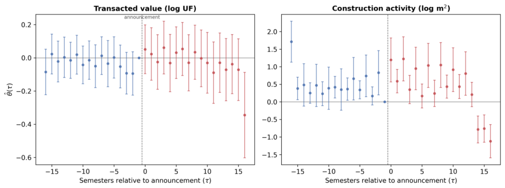
Figure 3.
HonestDiD identified sets. Top row: smoothness restriction ΔSD(M); bottom row: relative-magnitude restriction ΔRM(M̄). Left column: transacted value; right column: construction activity.
Figure 3.
HonestDiD identified sets. Top row: smoothness restriction ΔSD(M); bottom row: relative-magnitude restriction ΔRM(M̄). Left column: transacted value; right column: construction activity.
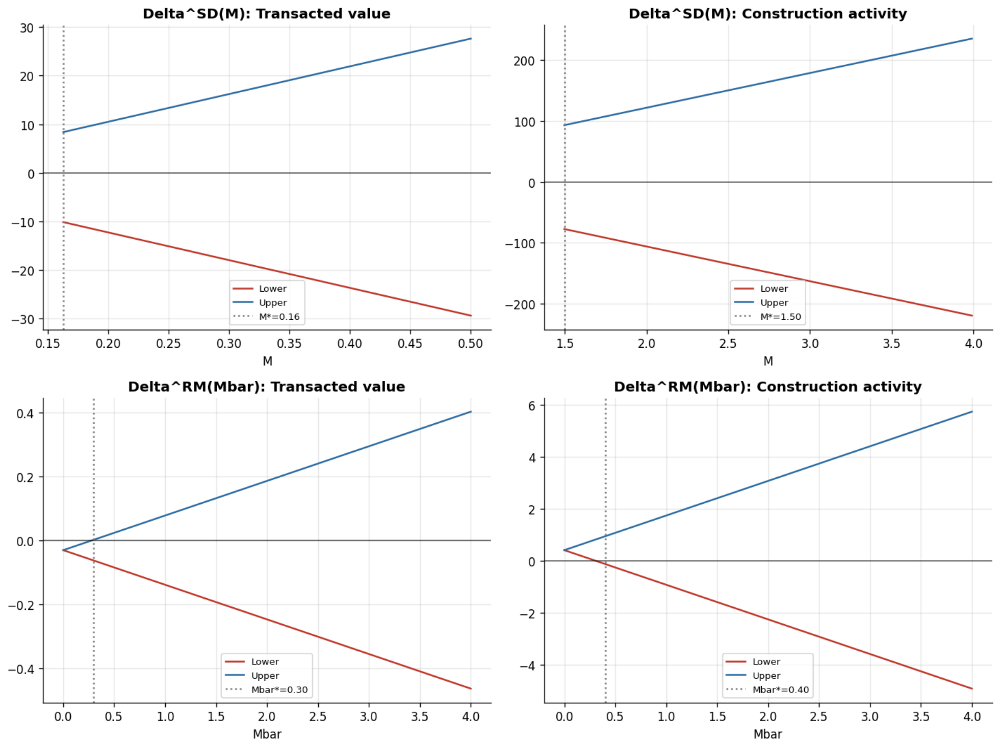
Figure 4.
Distribution of the anticipated accessibility premium across the Greater Santiago 34 universe (a) and mean anticipated uplift by IST-2024 quintile (b).
Figure 4.
Distribution of the anticipated accessibility premium across the Greater Santiago 34 universe (a) and mean anticipated uplift by IST-2024 quintile (b).
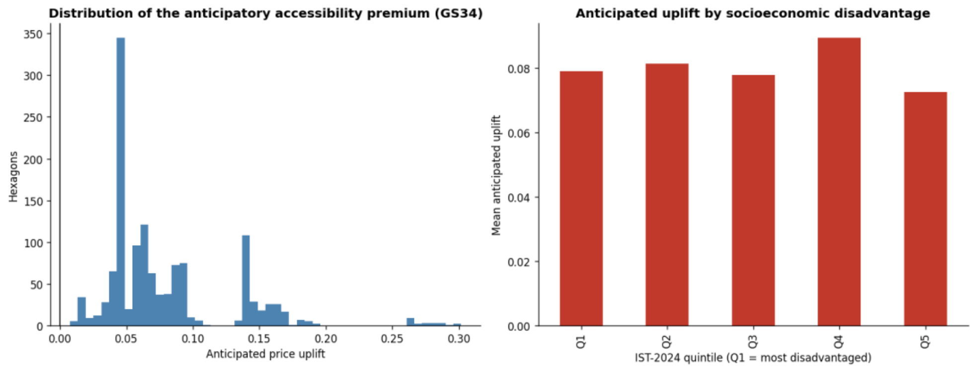
Table 1.
Data sources, their role in the pipeline, and temporal coverage.
| Source | Role | Level | Coverage |
|---|---|---|---|
| SII BRORGA2441N/NL | Cadastral stock and flow; land use and structural attributes | Construction line → parcel | Full registry to each parcel's build year; 2010S1–2025S2 |
| SII Form F2890 | Transaction registry (total UF value, land + construction) | Deed | Full registry from 1990; 2010–2025 |
| ComunasSII parcel table | Geocoding, address, assessed/commercial value | Parcel | Current |
| Metro station and line registries (operating and projected) | Station registry, announcement/opening dates, line geometry | Station/line | Current + historical |
| Street network, elevation nodes, bike-lane layer | Multimodal access network for the accessibility engine | Edge/node | Current |
| Censo 2024 cartography and tables | Population; IST-2024 socioeconomic-disadvantage components | Census block | 2024 |
| Encuesta Origen y Destino Santiago 2012 | Public-transport travel-time anchor (disclosed as a dated override) | Trip | 2012 |
| UF daily/annual series (Banco Central de Chile/SII) | Currency indexer for PESOS-denominated deeds | Day/year | 2010–2025 |
UF: Unidad de Fomento, Chile's inflation-indexed unit of account.
Table 2.
Verified treatment dates by line.
| Line | Primary Announcement | Alternative Milestone |
|---|---|---|
| L7 | 1 June 2017 (public address, President Bachelet) | — (single date, no ambiguity) |
| L8 | 1 June 2018 (first “Cuenta Pública,” President Piñera) | 27 February 2022 tender call (relaunched 5 September 2021, after the 9 March 2020 void) |
| L9 | 1 June 2018 (first “Cuenta Pública,” President Piñera) | 27 February 2022 tender call (relaunched 5 September 2021; new alignment 9 August 2023) |
Table 3.
Multi-level treatment roles.
| Role | Definition | Analogue in the Single-Event Design |
|---|---|---|
| TREAT_DIRECT | Hexagon within 1,000 m of a projected-line (L7/L8/L9) station | Direct-radius treatment |
| TREAT_COMUNA | Hexagon in a commune hosting a projected-line station, outside the 1,000 m catchment | Same-commune, indirect treatment |
| CONTROL_GS34 | Hexagon in the Greater-Santiago-34 universe, never within catchment of any projected line, and not in a commune whose own operating line (L3, L6) was built or opened inside the panel window | Nearby, untreated control |
| CONTROL_BORDE | Hexagon in the four SII-administrative edge communes straddling Greater Santiago, same L3/L6 exclusion applied | Distant, untreated control |
Table 4.
Hedonic capitalization elasticity with respect to gravity accessibility, current operating network.
Table 4.
Hedonic capitalization elasticity with respect to gravity accessibility, current operating network.
| Specification | log(Agrav) Coefficient (SE) | N |
|---|---|---|
| OLS, pooled (HC1 robust SE) | +0.0593 (0.0007) | 647,849 |
| OLS, commune fixed effects (HC1 robust SE) | +0.0262 (0.0019) | 647,849 |
| OLS, pooled (commune-clustered SE, primary specification) | +0.0593 (0.0099) | 647,849 |
Table 5.
Mean absolute SHAP feature importance, LightGBM diagnostic model.
| Feature | Mean |SHAP| |
|---|---|
| IST-2024 disadvantage index | 0.386 |
| log(structural floor area) | 0.277 |
| Building age | 0.182 |
| log(Agrav) | 0.068 |
Table 6.
Baseline TWFE estimates, all outcomes.
| Outcome | βdirect | p | βcomuna | p | N |
|---|---|---|---|---|---|
| Construction activity (total flow) | -0.117 | 0.569 | -0.073 | 0.501 | 67,072 |
| Construction of new parcels | -0.293 | 0.266 | -0.143 | 0.262 | 67,072 |
| Expansions of existing parcels | +0.206 | 0.235 | +0.084 | 0.322 | 67,072 |
| F2890 transactions (count) | -0.167 | 0.161 | -0.077 | 0.162 | 67,072 |
| Transacted value (log UF, land+construction) | +0.027 | 0.789 | +0.010 | 0.850 | 29,183 |
Table 7.
Callaway-Sant’Anna ATT(g,t), averaged across post-announcement horizons by cohort and outcome, with delta-method standard errors and approximate 95% confidence intervals.
Table 7.
Callaway-Sant’Anna ATT(g,t), averaged across post-announcement horizons by cohort and outcome, with delta-method standard errors and approximate 95% confidence intervals.
| Cohort | Outcome | Mean ATT(g,t) | SE | 95% CI | Horizons (t) |
|---|---|---|---|---|---|
| L7 (g = 2017S2) | Construction activity | -0.9348 | 0.1643 | [-1.257, -0.613] | 17 |
| L7 (g = 2017S2) | Transacted value | -0.2260 | 0.0521 | [-0.328, -0.124] | 17 |
| L8/L9 (g = 2018S1) | Construction activity | +1.1592 | 0.1651 | [+0.836, +1.483] | 7 |
| L8/L9 (g = 2018S1) | Transacted value | -0.0505 | 0.0273 | [-0.104, +0.003] | 16 |
Table 8.
Placebo test results.
| Type | Specification | β | p |
|---|---|---|---|
| Temporal | L7 fake date (2013S2) | -0.090 | 0.116 |
| Temporal | L8/L9 fake date (2014S1) | +0.014 | 0.604 |
| Spatial | Seed 11 | -0.048 | 0.483 |
| Spatial | Seed 22 | +0.008 | 0.902 |
| Spatial | Seed 33 | -0.060 | 0.382 |
Table 9.
Cluster bootstrap by cohort.
| Cohort | β | p (clustered) | p (bootstrap) | Clusters (G) | N |
|---|---|---|---|---|---|
| L7 (2017S2) | +0.177 | 0.709 | 0.669 | 811 | 14,813 |
| L8/L9 (2018S1) | +0.120 | 0.534 | 0.522 | 871 | 16,696 |
Table 10.
L8/L9 announcement-date robustness.
| Outcome | Primary (2018S1) β | p | Relaunch Milestone (2022S1) β | p |
|---|---|---|---|---|
| Construction activity | -0.410 | <0.001 | -0.610 | <0.001 |
| Transacted value | -0.081 | 0.028 | -0.099 | 0.018 |
Table 11.
Spillover-decay parameterization robustness.
| Parameterization | φecon (1/km) | Implied d1/2 (km) | βdirect | p |
|---|---|---|---|---|
| Stated d1/2 = 5 km | 0.1386 | 5.0 | +0.027 | 0.789 |
| β-derived (via VEL_COMERCIAL_KMH) | 0.0203 | 34.1 | +0.052 | 0.668 |
Table 14.
LISA local cluster classification, transacted price.
| Cluster type | Hexagons | Share |
|---|---|---|
| Not significant (NS) | 659 | 74.5% |
| Low-Low (LL) | 106 | 12.0% |
| High-High (HH) | 81 | 9.2% |
| Low-High (LH) | 22 | 2.5% |
| High-Low (HL) | 17 | 1.9% |
Table 15.
Equity triple-difference: differential anticipatory capitalization by disadvantage.
| Coefficient | Estimate | p-Value |
|---|---|---|
| βDDD (LowIST × treat_direct × post) | +0.2555 | <0.001 |
| βLowIST×post (region-wide low-IST trend) | +0.1733 | <0.001 |
| βtreat×post (treated, IST-unconditional) | -0.2683 | <0.001 |
Table 16.
Anticipated uplift by IST-2024 quintile (Q1 = most disadvantaged).
| Quintile | Mean | Median | N |
|---|---|---|---|
| Q1 | 7.91% | 5.31% | 251 |
| Q2 | 8.14% | 5.87% | 250 |
| Q3 | 7.78% | 6.52% | 250 |
| Q4 | 8.94% | 8.15% | 250 |
| Q5 | 7.26% | 7.01% | 251 |
N: number of hexagons in the Greater Santiago 34 universe per quintile.
Table 18.
High-risk hexagons by commune (top 10 by hexagon count).
| Commune | SII Code | Hexagons | Population |
|---|---|---|---|
| Puente Alto | 16301 | 44 | 210,614 |
| La Florida | 15128 | 15 | 98,102 |
| La Pintana | 16154 | 15 | 96,120 |
| La Granja | 16131 | 12 | 87,776 |
| Peñalolén | 15152 | 8 | 67,937 |
| San Ramón | 16153 | 7 | 56,095 |
| Quinta Normal | 14107 | 5 | 30,587 |
| San Joaquín | 16163 | 3 | 19,559 |
| Macul | 15151 | 1 | 6,835 |
| Pudahuel | 14111 | 6 | 1,945 |
Table 19.
Land-value-capture scenario comparison.
| Scenario | Disadvantaged Uplift | Advantaged Uplift | Equity Gap | Protected (Hexagons) |
|---|---|---|---|---|
| A: Status quo (ρ = 0%) | +8.02% | +7.91% | +0.11% | 0 |
| B: Land value capture (ρ = 30%) | +5.61% | +5.54% | +0.08% | 0 |
| C: Affordability lock (ρ = 20%, κ = 8%) | +5.11% | +6.33% | -1.22% | 116 (675,569 people) |
Table 20.
Sensitivity of the option premium to volatility (r and δ held fixed).
| σ Scaling | σ | Option Premium (V*/I) |
|---|---|---|
| ×0.50 | 0.0433 | 3.045× |
| ×0.75 | 0.0649 | 3.136× |
| ×1.00 (baseline) | 0.0865 | 3.261× |
| ×1.25 | 0.1082 | 3.416× |
| ×1.50 | 0.1298 | 3.599× |
Disclaimer/Publisher’s Note: The statements, opinions and data contained in all publications are solely those of the individual author(s) and contributor(s) and not of MDPI and/or the editor(s). MDPI and/or the editor(s) disclaim responsibility for any injury to people or property resulting from any ideas, methods, instructions or products referred to in the content. |
© 2026 by the authors. Licensee MDPI, Basel, Switzerland. This article is an open access article distributed under the terms and conditions of the Creative Commons Attribution (CC BY) license (http://creativecommons.org/licenses/by/4.0/).
Copyright: This open access article is published under a Creative Commons CC BY 4.0 license, which permit the free download, distribution, and reuse, provided that the author and preprint are cited in any reuse.