

Submitted:
25 August 2026
Posted:
31 August 2026
You are already at the latest version
Abstract
We construct the similarity structure of unsteady compressible two-fluid (Hall) plasma boundary layers with separate ion and electron temperatures. Combining the unsteady Howarth–Dorodnitsyn reduction of Stewartson \( [Q.~J.~Mech.~Appl.~Math.~\textbf{4}, 182 (1951)] \) with the diffusion-time similarity ansatz of Sun \( [Phys.~Fluids ~ \textbf{36}, 083616 (2024)] \), we obtain a closed system in \( (\eta,\tau) \) for the reduced stream function, flux function, out-of-plane field and velocity, and two temperatures. Three structural results organise the problem. First, the Hall transport operator is invariant under the Dorodnitsyn map: because the Hall coefficient \( \lambda=1/\mu_0 ne \) scales as the local temperature while the in-plane magnetic derivative \( B_\bot\!\cdot\!\nabla \) transforms with the inverse weight, the two cancel exactly, and the Hall term—together with the magnetic force per unit mass—takes precisely its incompressible form. The pressure gradient does not; it acquires the familiar factor \( \omega=T/T_r \). Second, variable density restores the electron-pressure (Biermann) term, which vanishes identically at constant density. We show it can never enter the in-plane flux equation, and that within a similarity solution at uniform pressure it still vanishes because all thermodynamic gradients are parallel; it survives only through the streamwise pressure gradient, where it reduces to the source \( \theta_{e,\eta}/2M^2 \) and generates a second, independent quadrupole. This Biermann quadrupole dominates the Hall quadrupole below \( M\simeq0.73 \) and exceeds it twelvefold at \( M^2=0.05 \). Third, exact Hall similarity requires a layer of constant thickness (\( m=1 \)) while exact compressible similarity requires constant edge Mach number (\( m=0 \)); the two are disjoint, so no exactly similar compressible two-fluid layer exists. The admissible families are a strongly heated stagnation-type layer, exact to all orders in \( \varepsilon_H \), and a compressible flat plate, exact in the thermodynamics and self-similar through \( O(\varepsilon_H) \), whose Hall subsystem remains a first-order pair with \( f\mapsto\omega f \). Further results: the change of type of the unsteady system is purely kinematic, both equations carrying \( 1-2\tau f_\eta, so \tau_{\rm crit}=1/2 \) independently of field strength, Mach number and wall condition; the Alfvénic degeneracy is not displaced by compressibility, because \( \omega\to1 \) at the layer edge where the transition is decided; an aligned frozen-in field destroys the Mach independence of the transformed flat-plate skin friction, by \( 38\% \) at \( M^2=0.7, M_e^2=16 \); a hot wall expels tangential flux, the wall field falling by a factor of \( 4.6 \) between \( M_e^2=0 \) and \( 16 \); and expansion cooling drives the electron temperature below its free-stream value when equipartition is weak. Numerical solutions reproduce Hiemenz, Blasius–Dorodnitsyn and the compressible recovery factor to six figures, and confirm the predicted \( O(\varepsilon_H^2) \) back-reaction over a sixteenfold range in \( \varepsilon_H \).
Keywords:
similarity structure
; unsteady compressible two-fluid plasma
; boundary layers
; Dorodnitsyn invariance
; Biermann quadrupole
1. Introduction
1.1. Background
The similarity solutions of the laminar boundary layer—Blasius, Falkner–Skan, Hiemenz, Rayleigh–Stokes—remain the fixed points around which the subject is organised [1,2,3,4,5]. Compressibility was absorbed into that framework by Howarth [6] and Dorodnitsyn [7], whose density-weighted normal coordinate converts the compressible momentum equation into something very close to its constant-density counterpart, and by Illingworth [8] and Stewartson [9], who extended the construction to flows with a pressure gradient. With the Chapman–Rubesin viscosity law [10] and the Crocco energy integral [11,12] this machinery yields the compressible Falkner–Skan–Dorodnitsyn system and, at a stagnation point with strong wall heat transfer, the variable-property solutions of Cohen and Reshotko [13]. The unsteady problem is older and harder: Stewartson’s analysis of the impulsively started plate [14,15] supplies a single variable interpolating between a diffusive Rayleigh layer and a convective Blasius layer, and reductions of this two-parameter type continue to be developed [16,17,18], with the Williams–Rhyne chart [19] providing the device that carries a solution through the region a forward march cannot enter.
For electrically conducting fluids the corresponding programme was carried out for single-fluid magnetohydrodynamics. Greenspan and Carrier [20], Sears [21], Sears and Resler [22] and Gribben [23] established the structure of aligned-field MHD boundary layers, in which an ambient field parallel to the free stream is swept into the layer and the character of the flow changes qualitatively as the Alfvén number passes through unity. The compressible version was treated by Rossow [24], Bleviss [25] and Bush [26], and the magneto-aerodynamic framework was set out by Resler and Sears [27]; general accounts of the single-fluid theory are given by Shercliff [46] and Davidson [45].
Plasmas, however, are not single fluids. Once the layer thickness approaches the ion inertial length , ions and electrons decouple: the field remains frozen to the electron fluid while the ions slip across it. The two-dimensional signature of this Hall regime is an out-of-plane field of quadrupolar symmetry, generated by the in-plane electron current and mediated by dispersive whistler dynamics. It was predicted by Sonnerup [28] and Terasawa [29], identified as the controlling ingredient of fast reconnection by Mandt, Denton and Drake [30], confirmed across the model hierarchy in the GEM challenge [31], analysed asymptotically by Uzdensky and Kulsrud [32], and measured in the laboratory and in space [33,34,35]. Any two-fluid boundary-layer theory must produce it. The four-field system that carries it is standard [36,37]; what is not standard is what happens to it when the density is allowed to vary.
1.2. What Is Missing, and What This Paper Supplies
What the literature does not contain is the two-fluid boundary layer at variable density. This is not a cosmetic extension, for three reasons that the body of the paper makes precise.
The first is that compressibility acts on the Hall coefficient itself. The quantity that multiplies every Hall term is inversely proportional to the number density, so in a layer whose wall is four times hotter than the free stream the Hall coefficient varies by the same factor across the layer, and the local ion inertial length by its square root. Neither variation can be scaled away. Whether the Hall physics is thereby amplified or suppressed is a question the constant-density theory cannot even pose.
The second is that variable density resurrects a term that constant-density theory annihilates. At uniform n the electron-pressure contribution to the induction equation is the curl of a gradient and vanishes identically. At variable n it is the Biermann battery [39,40], the canonical mechanism for generating magnetic field from nothing in astrophysical [41,42] and laser-produced plasmas. Since the Biermann source in two dimensions is directed out of the plane, it competes directly with the Hall stretching term for control of the quadrupole—the very structure that the two-fluid theory exists to predict.
The third is that compressibility and Hall physics impose competing similarity requirements. Constancy of the Hall group demands a layer of fixed thickness, because is an absolute length; constancy of the compressibility parameter demands a uniform external stream. In the single-fluid compressible theory only the second constraint is felt; in the incompressible two-fluid theory only the first. Together they are incompatible, and the resulting dichotomy dictates the entire architecture of the paper.
Contributions
- 1.
- 2.
- A weight-structure theorem (Section 3): under the Dorodnitsyn map the Hall operator, the magnetic force per unit mass and the Lorentz driving of the out-of-plane velocity are invariant, whereas the pressure gradient and the resistive terms are not.
- 3.
- A complete account of the Biermann term (Section 5.3): excluded exactly from the in-plane flux equation, excluded again by similarity at uniform pressure, and surviving only as a streamwise-pressure-gradient source that dominates the Hall quadrupole at low Alfvén number.
- 4.
- An exactness dichotomy (Theorem 2) and its two resolutions.
- 5.
- A kinematic change-of-type theorem for the unsteady system (Theorem 3) and a proof that the Alfvénic degeneracy is not displaced by compressibility (Theorem 4), both confirmed numerically.
2. Compressible Two-Fluid Model and Exact Planar Reductions
2.1. Species Equations and Closure
We take a quasineutral plasma of singly charged ions of mass and electrons of mass , with common number density n and mass density . The species momentum equations are
with the friction force and the viscous stresses. We adopt the standard boundary-layer closure: electron inertia is neglected, electron viscosity is neglected relative to ion viscosity, the ion stress is isotropic with dynamic viscosity , and the friction is resistive, [43,44]. Dropping in (2) and using with gives the generalised Ohm’s law [38]
in which the second and third terms on the right are the Hall and electron-pressure contributions. Throughout we write
so that and . In contrast to the constant-density theory, and are now fields: at constant pressure across the layer,
with T the mixture temperature defined below and the subscript r denoting a constant reference state. Equation (5) is the seed of most of what follows.
Because the two species carry separate temperatures, the equation of state is with
It is worth pausing on (6): the density weight that controls the Dorodnitsyn map is set by the mean of the two temperatures, so the geometric reduction of the compressible problem is itself a dual-temperature statement. Nothing analogous occurs in the single-fluid theory, and nothing at all occurs in the constant-density theory.
Two transport closures are needed, both direct analogues of Chapman–Rubesin:
We write , , with , and define
The viscous closure is the classical one and needs no further comment. The magnetic closure is a genuine modelling assumption and is the weakest link in the chain: Spitzer resistivity varies as , so (7)2 is not a fit to a real plasma but a device that makes the resistive operator conservative in the transformed plane. A one-parameter generalisation costs nothing—if then every resistive term below acquires the weight and no structural statement changes— and we return to the point in Section 10. All computations use .
2.2. Four Exact Statements About the Planar Problem
The following results delimit which terms can appear at all. Three of them are inherited unchanged from the constant-density theory; the second is reversed by compressibility, and that reversal is the physical heart of this paper.
(i) The Hall force does not act on the mixture.
Adding (1) and (2), the friction forces cancel by Newton’s third law and the electromagnetic forces sum to , so that with and ,
No term proportional to survives. The argument nowhere uses , so it carries over verbatim to compressible flow: the Hall force is internal to the electron–ion system and transfers momentum between species, not to the mixture. Adding a separate Hall force to (9) double counts . The Hall effect enters the dynamics only through (3).
(ii) The Biermann term survives, and only out of plane.
At constant n the electron-pressure term in (3) is a pure gradient, , and its curl vanishes identically. At variable n it does not:
where we used , so that . This is the Biermann battery. Two restrictions apply immediately. In a z-independent geometry , so the electron-pressure term makes no contribution whatever to the z-component of Ohm’s law and hence none to the in-plane flux equation: like the Hall term, and for the same topological reason, the Biermann term is an out-of-plane effect. And (10) requires misaligned density and electron-temperature gradients. We show in Section 5.3 that similarity itself imposes a further restriction, leaving the streamwise pressure gradient as the only surviving driver.
(iii) A strictly planar field contains no Hall physics.
Let be strictly planar, . Then is purely out of plane, so and the Hall term drops out of the flux equation identically; equivalently because . Solenoidality is all that is used, so again the statement is density-independent. Restoring gives and
A model that discards has discarded the Hall effect, however many factors of its equations appear to contain.
(iv) magnetic pressure cancels from streamwise momentum.
With , , , the transverse Lorentz component is , so the boundary-layer y-momentum balance gives
Eliminating p from the streamwise component, the terms cancel identically and
The same cancellation occurs in the free stream, so the elimination of is unaffected by . As in the constant-density case, this is the mechanical counterpart of (i): the Hall effect reaches streamwise momentum only indirectly, by modifying and .
2.3. Energy Pathways
From (3),
The Hall contribution vanishes identically because : the Hall electric field is perpendicular to the current and does no work, at variable density exactly as at constant density. Any formulation exhibiting an explicit “Hall heating” term has mis-assigned the electron work. The electron-pressure term, by contrast, is no longer a pure surface contribution: since ,
so the electron fluid compresses at a different rate from the ion fluid and does compressional work against that difference. Scaling shows the extra rate to be relative to , with defined in (35), so it enters at the same order as the Hall back-reaction on the in-plane field and is retained only there.
The species internal-energy equations are then
with and the equipartition exchange . Viscous heating is assigned to the ions and Ohmic heating to the electrons, as the closure requires; the compressional terms are new relative to the constant-density theory and, as Section 9 shows, are not small.
2.4. Boundary-Layer form and Free-Stream Compatibility
With x streamwise and y wall-normal, and with eliminated through (12), the system to be reduced is
together with (16)–(17). Here is a spatially uniform applied electric field arising from the residual gauge freedom , and
is the Biermann source from (10). The term in (21) is compressible in origin; combining it with the material derivative,
which identifies , not , as the quantity transported by the flow—a reformulation we shall find is exactly what the reduced equations want.
Outside the layer the plasma is ideal and the flux is frozen in, so . For a steady external state this integrates to
the compressible generalisation of the constant-density relation . The Alfvén number then obeys , so M is constant only when the edge density is. This is the first hint of the constraint proved in Section 4.
3. The Unsteady Dorodnitsyn Reduction and Its Weight Structure
3.1. Stewartson’s Lemma
Define the Dorodnitsyn variable and map with , and
In unsteady flow depends on t through and the naive stream function fails. The remedy, due to Stewartson [14], is to absorb into the transformed normal velocity: with
the material derivative and the continuity equation take the incompressible forms
so that a transformed stream function exists with , , even though . We take (28) as given; the proof is a two-line chain-rule calculation reproduced in many places and adds nothing here.
3.2. The Magnetic Bracket
The corresponding statement for the magnetic operator does not appear to have been recorded, and it is what makes the two-fluid reduction tractable.
Lemma 1
(magnetic bracket). For any field F, with and ,
where is the Poisson bracket in the transformed plane .
Proof.
Since we have , and . Hence
and the two terms in cancel. □
The cancellation of is the exact magnetic analogue of the cancellation of in Stewartson’s lemma, and it means that—as with the mass flux—one never needs explicitly.
3.3. What carries the density weight and what does not
Theorem 1
- (a)
- inertia and the viscous term take their incompressible form, ;
- (b)
- the pressure-gradient term acquires the weight ;
- (c)
- the in-plane magnetic force per unit mass, the Hall transport term, and the Lorentz driving of areweight-free:
- (d)
- the resistive terms are not: and ;
- (e)
- the whole right-hand side of the equation carries the single weight , consistent with (24).
Proof. (a) is classical: with , and division by leaves . (b) follows because dividing the pressure gradient by produces . For (c), combine Lemma 1 with : the two weights cancel. The same cancellation occurs for the Hall term because by (5), so . (d) is a direct computation using . (e) follows on dividing (21) by and using (24). □
Part (c) deserves emphasis. That the magnetic force per unit mass should be Dorodnitsyn-invariant is intelligible: behaves like a material line element, so the ratio of magnetic tension to inertia is blind to the expansion. That the Hall term should be equally invariant is less obvious, and is a coincidence of exponents: the Hall coefficient grows as precisely as fast as the magnetic derivative operator shrinks. The practical consequence is that every Hall term below is literally identical to its constant-density counterpart, and all compressible modification of the two-fluid coupling enters through the resistive weights, through the compressional terms, and through the Biermann source.
It is worth contrasting this with the low-magnetic-Reynolds-number problem, in which an externally applied field exerts a drag that carries the full weight . There the Lorentz term is a body force imposed from outside and its acceleration per unit mass is enhanced in the hot, light gas; here the field is frozen to the fluid and shares its expansion, and the enhancement disappears. The two problems behave oppositely for a reason that is entirely kinematic.
Finally, the local Hall length in transformed units follows from (5): a physical length ℓ corresponds to in , so
which is smaller in the hot near-wall gas than the constant-density estimate.
4. The Similarity Ansatz and an Exactness Dichotomy
4.1. The Two-Parameter Map
Following Sun [18], and now in the Dorodnitsyn plane, introduce
and write the fields as
Two derived profiles occur so often that they deserve names:
The distinction between and is purely compressible and is easy to lose: measures flux per unit mass coordinate, the physical tangential field. They coincide only where .
Balancing the Hall source in (21) against advection fixes the amplitude of and defines the Hall similarity parameter,
and balancing the Lorentz force against inertia in (22) gives , as anticipated in (33). Note that the prefactors in (33) are definitions, not approximations: no expansion in has been made.
4.2. The Dichotomy
Autonomy of the reduced system requires every dimensionless group to be independent of x. The groups are the geometric pair
together with M, , , , and the compressibility parameter that fixes the relation between static and total enthalpy at the edge.
Theorem 2
(incompatibility of Hall and compressible exactness). Within the power-law family there is no member for which the Hall group and the compressibility parameter Θ are simultaneously independent of x.
Proof.
Constancy of forces , because is an absolute length fixed by the reference density alone and cannot be rescaled by any choice of external flow, and M is already required constant. Then and requires , i.e. after absorbing a shift of origin (the degenerate alternative with gives the one-dimensional Rayleigh layer).
Constancy of requires a constant edge Mach number. For an isentropic outer flow driven by the edge temperature satisfies , so is constant only if is, i.e. . The same conclusion follows independently from (25): is constant only if the edge density is, which for an isentropic outer flow again requires .
The two requirements are and and cannot both hold. □
The theorem is sharper than its single-fluid ancestors because it involves two absolute constraints pulling in opposite directions, and it is constructive: it tells us there are exactly two things to do, and we do both.
Class B (stagnation-type, ).
Take , , , so that carries no residual x dependence and is exactly constant. Exactness in is recovered in the distinguished limit
in which the external flow is effectively incompressible—so , and p are uniform and (25) gives —while the layer carries an order-unity density variation supplied entirely by wall heat transfer. This is precisely the setting of the classical variable-property stagnation-point solutions [13], and it is not a weak limit: at the near-wall density is a quarter of its free-stream value. Dissipation is in this limit and is treated as a regular perturbation in Appendix C.
Class A (flat plate, ).
Take , , , whence , and is Stewartson’s variable. Here , M and are exactly constant and the compressible thermodynamics, including dissipation at arbitrary Mach number, is exactly similar. The Hall group is not: , and similarity survives exactly through , breaking only at .
Each family is exact in the sector the other cannot reach. Together they bracket the problem.
5. Class B: The Strongly Heated Stagnation-Type Layer
5.1. Reduction
With constant, and are independent of x, the operator generated by never acts, and the reduction closes term by term. The kinematics are
and the dilatation, which will appear repeatedly, is obtained from as
reducing in steady flow to . The full substitutions are given in Appendix A. The result is the master system
with and the Eckert parameter of the distinguished limit (37). Setting makes , , , and (40)–(43) collapse to the constant-density two-fluid system; setting and leaves the compressible aligned-field MHD layer.
Several features repay attention.
(i) The pressure gradient is the only weighted mechanical term. In (40) the buoyancy-like combination replaces , exactly as in single-fluid compressible theory, while the magnetic group contains only through the same channel: and at the edge, so the group vanishes there as it must.
(ii) The Hall terms are literally unchanged. The combination appearing in (41) and (43) is identical to its constant-density form—not merely analogous. This is Theorem 1(c) in action, and it is the reason the compressible problem remains tractable at arbitrary .
(iii) The perfect-derivative structure of the Hall source is broken. At constant density the stretching source in (42) is , the exact -derivative of the magnetic group that supplies the tension in the momentum equation. Here, using ,
so the structural link with the tension group survives but acquires a defect proportional to the density gradient. The quadrupole is therefore driven partly by the gradient of the magnetic tension, as before, and partly by the temperature gradient acting on the tangential field alone.
(iv) Compression work is an term in the thermal problem. The terms in (44)–(45) are of the same order as conduction, not a correction to it. Summing the two equations with and using (39) returns , the standard compressible enthalpy equation, which is the check that the compressional bookkeeping is consistent.
5.2. Boundary Conditions
At an impermeable, no-slip wall, and matching to the free stream,
The system order is , matching the thirteen conditions. The condition states that the wall is a magnetic flux surface, ; the condition —rather than —is the one place where the distinction in (34) matters for the formulation, and using the wrong one displaces the whole magnetic solution. We adopt the insulating wall model, , which gives exactly and requires no subsidiary expansion. The wall tangential field and the wall current are outputs.
The role of is as at constant density. A uniform enters (41) as an inhomogeneous term , which depends on x unless ; working with the uncurled, second-order form of the flux equation imposes this automatically.
5.3. The Biermann Source
We now evaluate (23) inside the similarity family, which is where the interesting restriction appears.
Proposition 1
(similarity annihilates the Biermann term at uniform pressure). If the pressure is uniform, so that with T a function of the similarity variable alone, then and .
Proof.
At uniform p, n depends on position only through T, and both T and are functions of alone. Hence and are parallel and their cross product vanishes. □
The proposition disposes of Class A immediately: a flat plate has no streamwise pressure gradient, so the Biermann battery is identically inoperative there, however strong the heating. It also shows that the effect is not simply “switched on by compressibility”; what switches it on is the streamwise pressure gradient, which tilts the isopycnals away from the isotherms.
In Class B the pressure is not quite uniform. Eliminating as in (12) and evaluating at the edge, the magnetic contributions cancel between and the edge momentum balance, leaving
Writing and using ,
which on division by the reference scale gives, with and ,
which is the last term in (42). Three properties of this source are worth stating explicitly.
It scales correctly. exactly as does, so the Biermann battery is compatible with Class-B similarity rather than merely tolerated by it.
It does not vanish in the distinguished limit. Although (48) is itself , the reference scale against which it is measured is in the same way, and the ratio (50) is free of . The Biermann quadrupole is therefore a robust feature of the exactly similar Class-B layer, not a high-Mach-number curiosity.
It is independent of and diverges as . Because h was normalised by , a source of size means a physical field . This is as it should be: the Biermann battery needs no seed field, whereas Hall stretching requires one, so at weak field the battery must win. Comparing (50) with the Hall source (46) predicts a crossover at
which Section 9 confirms at for .
For orientation in physical terms, the ratio of the Biermann to the Hall source can be written as , the electron plasma beta, times the relative temperature variation along a field line and a factor measuring the strength of the streamwise pressure gradient. Low- layers make Hall quadrupoles; high- layers make Biermann quadrupoles.
5.4. Displacement Identity and Integral Relations
Writing and as , the far-field limit of (41) is obtained by noting that , , there, so that
in the steady state. Compressibility does not modify this: the identity lives entirely in the outer region, where the density perturbation has died. The general solution of the far-field flux equation is plus a solution decaying as , and selects ; no additive constant is admissible. Equation (52) is a sharp, falsifiable prediction of the formulation and we use it as a numerical check.
Integrating (40) once in the steady state, with the momentum and displacement thicknesses
and their magnetic counterparts formed with , one obtains a von Kármán relation of the usual type in which the wall stress is the difference between a hydrodynamic and a magnetic thickness combination weighted by , augmented by —the thermal expansion integral, which is the only new term and which measures the extra momentum flux the layer must accommodate because the near-wall gas is light.
6. Class A: The Compressible Flat Plate
6.1. Reduction and Master System
For Class A, and does act. Carrying out the substitutions (Appendix B), all terms proportional to cancel identically in every equation—the mechanism by which the Blasius-type layer remains autonomous—and one obtains
where and we have taken . Equation (58) is the mixture equation; the species split is obtained by adding the difference equation for , in which the ion viscous and electron Ohmic sources appear with opposite signs and equipartition supplies the damping.
Three points. First, (54) reduces at to irrespective of : the classical Mach independence of the transformed flat-plate momentum problem. With it does not, because the magnetic term samples the temperature profile directly. An aligned frozen-in field therefore destroys the Mach independence of the transformed skin friction. The same conclusion is reached in the low- applied-field problem, but by the opposite route—there through the weight on the Lorentz drag, here through the dilution of a frozen-in field by expansion—and the mechanisms should not be conflated.
Second, the out-of-plane pair (56)–(57) is in divergence form, and remains so under compressibility with the single modification . Integrating once from to ∞ and using decay,
with : the Hall subsystem of the Blasius-type layer is a first-order initial-value problem, a considerable simplification with no single-fluid analogue and one that compressibility does not spoil. Evaluating (59) at the wall, where , gives identically for every decaying solution: the perfectly conducting wall condition is redundant, as at constant density, and the insulating condition is the non-degenerate choice.
Third, since enters (55)–(56) only at , the Hall-generated fields of the growing layer are exactly self-similar through first order,
with universal profiles. Hall physics in a growing layer is a leading-edge phenomenon, significant where , i.e. for
in which compressibility enters only through the Chapman–Rubesin constant. In physical coordinates the picture is less tidy: the layer is thicker by but the gas is lighter and correspondingly larger, and the two effects partially compensate, with the residual given by (31).
6.2. The change of type is purely kinematic
Collecting the -derivatives in (54)–(55),
and differentiating the second with respect to shows that carries the same factor.
Theorem 3
(kinematic threshold). The Class-A system is well posed as an initial-value problem in τ so long as throughout the layer. Since at the edge, the first loss of parabolicity occurs there at
independently of M, , , the edge Mach number, the Prandtl numbers and the wall thermal condition.
Proof.
The -principal symbol of the system (62) in the unknowns is times the identity, plus terms of lower order in the -derivative. Neither M nor , , , nor the boundary data appears in that coefficient, and the supremum of over the layer is unity. □
This is the analytical content of Stewartson’s obstruction, now shown to be untouched by either the field or the two-fluid physics: at , that is at , the direction in which information propagates in reverses, and no forward march can succeed beyond it. The remedy is the Williams–Rhyne chart [19], , , , in which both ends are characteristic and the whole history from impulsive start to steady state is obtained as one boundary-value problem; at one recovers , i.e. , and at the steady system (54)–(58). Since neither field nor compressibility appears at leading order as —the diffusion terms are while all others are —the impulsive start is universal: the quadrupole is born from a Rayleigh state that knows nothing of M, or . We formulate the chart here but do not compute in it; the global unsteady solution is left for future work, and we are careful below to present only steady results.
7. Two Structural Consequences
7.1. The Alfvénic Degeneracy Is Not Displaced
At constant density the aligned-field layer degenerates at , : the equipartitioned field-aligned state forces and no boundary layer exists [22]. One might expect variable density to move this point, since the alignment condition becomes and is no longer compatible with .
Theorem 4.
The Alfvénic critical point of the compressible two-fluid layer is , independently of the wall temperature ratio.
Proof
(Argument). Set , with small in the outer region, where and hence . Linearising (40)–(41) there gives
which is exactly the constant-density far-field system, whose determinant vanishes at . The transition is decided in the outer region, where the density perturbation has died; the interior, however strongly heated, cannot move it. □
We label this an argument rather than a proof because it establishes only that the far-field character changes at ; that this coincides with the vanishing of the wall stress is a global statement which we verify numerically in Section 9 over . The result is worth stating precisely because the naive expectation— that a hot, light near-wall gas should be easier for magnetic tension to arrest—is wrong.
7.2. The hierarchy in
Equations (40)–(43) generate the same three-tier hierarchy as at constant density, now with compressible coefficients. At , obey the compressible aligned-field MHD problem with . At , obey the linear, -independent problem (42)–(43) evaluated on that base state, forced by (46) and by the Biermann source; the quadrupole profile is universal and its amplitude linear in . At the back-reaction on the in-plane fields appears. This is the precise sense in which the Hall effect is a second-order correction to the in-plane fields but a first-order effect in its own right, and Section 9 verifies it over a sixteenfold range in at .
The whistler branch that mediates the coupling, , survives locally with the local and ; expressed through (31) its similarity wavenumber is , so the dispersive scale contracts in the hot gas. The behaviour at small scales makes the semi-discrete Hall coupling a stiff fourth-order operator, and any unsteady integration of (40)–(45) must be implicit.
8. Numerical Method
The steady Class-B problem (40)–(45) is a thirteenth-order two-point boundary-value problem. We carry the state , using so that rather than is a primitive variable— which enforces the correct edge condition automatically and avoids differentiating unnecessarily. One structural difficulty must be handled: (42) requires , which contains ; differentiating (41) expresses in terms of , which (42) supplies. The coupling is linear and is eliminated in closed form,
with K given in Appendix D; the bracket is strictly positive, so the elimination never fails. Solution is by collocation [50] with adaptive mesh refinement (scipy.integrate.solve_bvp [51]) to a tolerance of – on with and 1201–2001 initial nodes, continued in , then , then . Continuation is not optional: without it the solver readily jumps to spurious branches with at moderate , and all results reported here were checked for pointwise positivity of .
The Class-A problem (54)–(58) is ninth order in the steady state and is solved by the same method with ; the analogous elimination is needed for against .
Two remarks on accuracy. The wall quantities and are converged to eight significant figures and are insensitive to beyond 16. The displacement constants are not: in the outer region the advective terms are individually and nearly cancel, so and inherit a truncation error that falls with rather than with mesh refinement. The identity (52) is satisfied to at , at 16 and at 20, with mesh refinement from 1201 to 3201 nodes changing nothing at any of these; we quote to five figures accordingly and regard the convergence of with domain size as the meaningful check.
9. Results
Throughout, .
9.1. Validation
Table 1 collects the checks against independently known limits. Setting makes an exact solution of (44)–(45), hence , and the Class-B system must collapse onto the constant-density two-fluid problem; at it must further reduce to Hiemenz flow. We obtain and , the tabulated values. The Class-A system at must reduce to Blasius in the normalisation , giving and a displacement constant ; we obtain and .
The thermal side is checked against the classical compressible flat plate. At the transformed wall stress must be independent of , and we find at to all digits shown. The adiabatic recovery factor at comes out against the approximation ; the small residual is not numerical error but the known departure of the exact solution from , and its sign and magnitude agree with the standard tabulations [49].
9.2. The Heated Stagnation-Type Layer
Table 2 and Fig. Figure 1 give the base state as the wall temperature ratio is varied at fixed , , .
Three effects are visible. First, heating raises the wall stress substantially, by between and 4. Because while , the weights cancel and is the physical skin friction in units of ; the increase is real and is driven by the enhanced pressure-gradient term of (40).
Second, the wall tangential field collapses, falling from to . This is flux expulsion by expansion: the frozen-in field shares the dilation of the gas, so a hot layer carries the same flux over a greater thickness at lower field strength. It is the magnetic counterpart of the familiar compressible thickening, and it is the reason the magnetic tension weakens even though M is held fixed.
Third, and least expected, the quadrupole amplitude is non-monotonic, falling to a minimum near and then rising by a factor of nearly four by , while its peak jumps from to . The two branches of this behaviour are the two sources: Hall stretching, which peaks in the outer part of the magnetic layer and is weakened by flux expulsion, and the Biermann battery, which is proportional to and is therefore largest at the wall. We isolate them next.
9.3. Biermann Against Hall
Figure 2 and Table 3 compare the full solution with one in which the Biermann source of (50) is deleted and everything else retained.
The predicted structure is reproduced exactly. The Hall-only amplitude varies by only across a sixteenfold range of , as it must, since and not M sets it. The full amplitude tracks at small M, crossing the Hall value at —to be compared with the estimate (51), which gives and, with the computed wall gradient at , . At the Biermann quadrupole exceeds the Hall quadrupole by a factor of . Its spatial signature differs too: because it is driven by the electron temperature gradient rather than by the curvature of the magnetic profile, it peaks much closer to the wall, as Fig. Figure 2(a) shows.
This is the central quantitative result of the paper. In a compressible layer with a streamwise pressure gradient and appreciable wall heat transfer, the out-of-plane field is not in general the Hall quadrupole of reconnection theory, and interpreting a measured as a Hall signature without first estimating the Biermann contribution will overstate by whatever factor Table 3 supplies.
9.4. Alfvénic Approach and the Hierarchy
Figure 3(a) shows against for . Every curve falls to zero at , and continuation fails there in every case; the wall stress at is , , and for , 1, 2, 4 respectively, a spread of against a hundredfold spread in the driving. Theorem 4 is confirmed: the critical Alfvén number is not moved by heating, only the approach to it.
Figure 3(b) tests the hierarchy. Holding , , and reducing from to , the departures of the wall quantities from their values follow a clean power law of slope 2, with prefactors
constant to better than over the whole range, while the normalised quadrupole amplitude changes by only . Both halves of the hierarchy—an back-reaction and an -independent quadrupole shape—therefore survive compressibility intact.
9.5. Dual-Temperature Structure and Expansion Cooling
At the two species are decoupled and their profiles differ by more than a factor of two at , since the ion thermal layer is thick () and the electron layer thin. As grows the profiles are driven together and the single-temperature limit is approached, the ion wall flux rising by and the electron flux falling by while the total changes by .
The feature we did not anticipate is the electron undershoot: at small the electron temperature falls below its free-stream value in the outer part of the layer, reaching at , despite a wall three times hotter than the free stream and no cooling anywhere in the problem. The mechanism is the compression term of (45). With a hot wall and , so (39) gives : fluid carried from the cool outer region into the hot near-wall region expands and does work against its own pressure. A species whose thermal diffusivity is too small to conduct the deficit away cools accordingly. The effect is absent from any constant-density formulation, where , and it is selective—it acts on the poorly diffusing species only—so it is a genuine dual-temperature signature of compressibility rather than a mixture property. Note also that the quadrupole amplitude falls by across the range, through the Biermann source’s dependence on alone: equipartition, which is a purely thermal process, thereby controls a magnetic observable.
9.6. The Compressible Flat Plate
The loss of Mach independence is the headline. With the transformed wall stress is at every ; with , , , it falls between and by , , and respectively. The mechanism is transparent in Fig. Figure 5(b): the wall tangential field drops from to , a factor of , as dissipative heating expands the near-wall gas and dilutes the frozen-in flux. Weaker near-wall field means weaker magnetic tension, so the field brakes the layer less effectively and—since the aligned field reduces skin friction—the stress falls further below its field-free value the hotter the layer becomes.
The quadrupole is comparatively robust, varying by only over the same range and peaking near : the reduction in that weakens the Hall source is partly offset by the outward migration of the magnetic layer, and the Biermann battery is absent by Proposition 1. Finally, the wall stress is almost independent of , changing by over at , because in Class A the Hall feedback reaches the momentum equation only through the doubly indirect chain ; the wall field, by contrast, responds strongly, rising from to .
10. Applicability, and Where the Description Fails
The results rest on assumptions that should be separated by severity.
Transport closures. The viscous law is the classical Chapman–Rubesin approximation and carries the error already accepted throughout compressible boundary-layer theory. The magnetic and thermal analogues in (7) are weaker. Spitzer resistivity varies as and the Braginskii conductivities are strongly anisotropic in a magnetised plasma, only partially captured by using perpendicular coefficients. A power law is absorbed at no cost—every resistive term acquires the weight —and since for a real plasma the hot near-wall gas would be more conducting than our baseline, sharpening the current layer and strengthening the Hall source. The quantitative values at should be read as indicative of trend.
The distinguished limit of Class B. Exactness there requires , so the dissipation terms are formally and enter as the regular perturbation of Appendix C. This is the classical framework for variable-property stagnation-point layers and is not restrictive for the density ratios we explore, but it does mean that Class-B results should not be quoted for a hypersonic stagnation region without carrying the problem explicitly.
Two temperatures, one density. We have allowed but enforced quasineutrality and a single mass density, so charge separation, ambipolar fields and the thermal force are excluded, and is imposed on the mixture. Electron inertia is neglected, so the electron skin depth and the associated sub- structure are absent; its restoration would remove the unbounded whistler frequency and, incidentally, the stiffness noted above.
Regime of validity. The tension identified in the constant-density theory persists: with and , , so collisional plasmas large compared with are generically of high Reynolds number and the two requirements conflict. Compressibility does not relieve this, but it does add a route not available before: because , a strongly heated near-wall region has a locally enhanced Hall coefficient, so the effective two-fluid parameter is larger at the wall than the edge-based estimate suggests, by in and in .
Laminar, and stable by assumption. At the wall temperature ratios explored here a real high-speed layer would be interacting with transition, and nothing in this paper addresses whether the states exhibited are selected. We regard a linear stability analysis of these base states—in which the Mack modes of the compressible layer and the whistler branch of the two-fluid coupling compete—as the natural next step, and deliberately have not attempted it here.
11. Conclusions
We have derived the similarity structure of the unsteady compressible two-fluid plasma boundary layer and solved the resulting steady states.
The organising structural result is that the Dorodnitsyn map treats the two-fluid physics more kindly than one has any right to expect. Because the Hall coefficient is inversely proportional to density while the in-plane magnetic derivative carries the reciprocal weight, the Hall transport operator—and with it the magnetic force per unit mass and the Lorentz driving of the out-of-plane velocity—is invariant under the transformation, and takes exactly its constant-density form. Compressibility reaches the two-fluid coupling only through the resistive weights, through compression work, and through a term that constant-density theory does not possess at all.
That term is the Biermann battery. We showed that it can never enter the in-plane flux equation, that similarity at uniform pressure annihilates it because all thermodynamic gradients become parallel, and that it therefore survives only as a streamwise-pressure-gradient source, reducing to . It is absent from a flat plate and unavoidable at a stagnation point, it needs no seed field and consequently dominates at low Alfvén number, and it generates a quadrupole that peaks much nearer the wall than the Hall quadrupole does. At and it is the larger of the two by a factor of ; the two are equal at , in agreement with the analytical estimate . Any interpretation of a measured out-of-plane field as a Hall signature in a layer with heat transfer and a pressure gradient must dispose of this contribution first.
Exact similarity of the compressible two-fluid problem is impossible: the Hall group requires a layer of constant thickness and the compressibility parameter requires a uniform external stream. The two resolutions are complementary and we developed both—a stagnation-type layer, exact to all orders in and carrying order-unity density variation supplied by wall heat transfer, and a compressible flat plate, exact in its thermodynamics at arbitrary Mach number and self-similar through , whose Hall subsystem remains a first-order pair under the single substitution .
The unsteady system changes type at for purely kinematic reasons, both equations carrying the factor , so Stewartson’s obstruction is untouched by the field, the Mach number, the Prandtl numbers or the wall condition; and since neither field nor compressibility is felt at the impulsive start, the quadrupole is born from a universal Rayleigh state.
Numerically: the Alfvénic degeneracy remains at for wall temperature ratios from to 4, because the transition is decided in the outer region where the density perturbation has died; a hot wall raises the stagnation-point skin friction by while expelling tangential flux and reducing the wall field by ; an aligned frozen-in field destroys the Mach independence of the transformed flat-plate skin friction, by at and , through the dilution of the near-wall field by dissipative heating; and expansion cooling drives the electron temperature below its free-stream value when equipartition is weak, an effect that no constant-density formulation can contain.
Natural extensions are finite electron inertia; an ionisation model coupling and self-consistently to the thermal field; the global unsteady solution in the Williams–Rhyne chart, which the change-of-type theorem shows to be necessary rather than merely convenient; and the stability of these states, where the interaction of the whistler branch with the compressible instability modes seems likely to be delicate.
Acknowledgments
My investigations into the boundary layers started from my tenure as a professor at the Cape Peninsula University of Technology (CPUT), South Africa. I am profoundly grateful to CPUT for granting me complete academic autonomy to advance this research agenda. This vital institutional support laid the foundation for the principal conclusions presented in this manuscript. I also extend my deepest gratitude to former Vice-Chancellor (now Chancellor) Prof. Brian Figaji, and former Deputy Vice-Chancellors Prof. J. A. Tromp and Prof. Anthony Staak, for their generous support and endorsement. Further academic support was provided by Xi’an University of Architecture and Technology (XAUAT) and the Beijing Institute of Nanoenergy and Nanosystems (BINN), Chinese Academy of Sciences. I sincerely thank former XAUAT President Prof. Xiao-Jun Liu and current President Prof. Xiang-Mo Zhao, along with BINN Founding Director Prof. Zhong Lin Wang, for their unwavering encouragement and invaluable resource support throughout this study.
Data Availability Statement
The data supporting the findings of this study are available from the corresponding author upon reasonable request.
Conflicts of Interest
The authors declare that there are no competing financial interests.
Appendix A. Detailed Class-B Reduction
With constant, and are independent of x, so acts only on explicit prefactors. From and ,
Momentum. Term by term, using Theorem 1,
with the edge term . Dividing by gives (40). Every term is proportional to x, which is why the reduction closes.
Flux., , , and by Theorem 1(c) . The resistive term is . Dividing by , the Hall coefficient is and the resistive coefficient is , giving (41).
Out-of-plane field. With ,
whose coefficient after division by is unity; (46) then puts it in the form quoted. The stretching term is and the resistive term . Adding the Biermann source (50) and using (24) for the left-hand side gives (42).
Out-of-plane velocity. The Lorentz term is and the viscous coefficient is ; dividing by gives (43). This calculation fixes the normalisation : any other choice leaves in two places instead of one.
Energy. Dividing (16) by turns the compression term into and, with constant, the conduction term into ; the material derivative is and . The dissipation terms are weight-free, since , and combine to ; they are collected in Appendix C.
Appendix B. Class-A Algebra
For Class A, and
with . In the steady flux equation,
and the terms in cancel; the same cancellation occurs in every equation and is the mechanism by which Class A remains autonomous. For the out-of-plane fields, the exponent in is what produces the divergence form: with ,
and the compressible correction converts into , which is (56).
Appendix C. The O(Ec) DISSIPATIVE problem for Class B
Dissipation scales as in Class B, so we write with . The leading problem is (44)–(45) without sources and is exactly similar; it alone determines and hence the entire reduction. At , the streamwise advection of the correction contributes , so the correction problem is
a linear inhomogeneous pair with homogeneous boundary conditions, in which is the dilatation perturbation induced by . The ion source is viscous and the electron source Ohmic, in the ratio , so the two species are heated by different profiles peaking at different heights; the terms are the only channel by which two-fluid physics alters the partition of heating between species.
Appendix D. Numerical Details
The right-hand side of (65) is
obtained by differentiating (41) to give and substituting into , with .
Steady Class-B solutions use (raised to 32 near ), 1201–2001 initial nodes and tolerance –, with continuation steps above and ; coarser continuation diverges and can be mistaken for a genuine breakdown of the branch. Class-A solutions use and 1201 nodes. Grid refinement from 1201 to 3201 nodes changes the reported wall quantities in the eighth decimal.
The first checks to run when reproducing this work are, in order: Hiemenz ( at , ); Blasius–Dorodnitsyn ( for Class A); the collapse of the whole Class-B system to its constant-density form when ; the identity ; and the recovery factor at . A reader who obtains for the Class-A wall stress has used the conventional Blasius normalisation rather than .
References
- H. Schlichting and K. Gersten, Boundary-Layer Theory, 9th ed. (Springer, Berlin, 2017).
- L. Rosenhead (ed.), Laminar Boundary Layers (Oxford University Press, Oxford, 1963).
- H. Blasius, Grenzschichten in Flüssigkeiten mit kleiner Reibung, Z. Math. Phys. 56, 1 (1908).
- V. M. Falkner and S. W. Skan, Some approximate solutions of the boundary layer equations, Philos. Mag. 12, 865 (1931). [CrossRef]
- K. Hiemenz, Die Grenzschicht an einem in den gleichförmigen Flüssigkeitsstrom eingetauchten geraden Kreiszylinder, Dinglers Polytech. J. 326, 321 (1911).
- L. Howarth, Concerning the effect of compressibility on laminar boundary layers and their separation, Proc. R. Soc. London, Ser. A 194, 16 (1948).
- A. A. Dorodnitsyn, Boundary layer in a compressible gas, Prikl. Mat. Mekh. 6, 449 (1942).
- C. R. Illingworth, Steady flow in the laminar boundary layer of a gas, Proc. R. Soc. London, Ser. A 199, 533 (1949). [CrossRef]
- K. Stewartson, The Theory of Laminar Boundary Layers in Compressible Fluids (Oxford University Press, Oxford, 1964).
- D. R. Chapman and M. W. Rubesin, Temperature and velocity profiles in the compressible laminar boundary layer with arbitrary distribution of surface temperature, J. Aeronaut. Sci. 16, 547 (1949). [CrossRef]
- L. Crocco, Sulla trasmissione del calore da una lamina piana a un fluido scorrente ad alta velocità, L’Aerotecnica 12, 181 (1932).
- E. R. van Driest, Investigation of laminar boundary layer in compressible fluids using the Crocco method, NACA Technical Note No. 2597 (1952).
- C. B. Cohen and E. Reshotko, Similar solutions for the compressible laminar boundary layer with heat transfer and pressure gradient, NACA Report 1293 (1956).
- K. Stewartson, On the impulsive motion of a flat plate in a viscous fluid, Q. J. Mech. Appl. Math. 4, 182 (1951). [CrossRef]
- K. Stewartson, The theory of unsteady laminar boundary layers, Adv. Appl. Mech. 6, 1 (1960). [CrossRef]
- N. Riley, Unsteady laminar boundary layers, SIAM Rev. 17, 274 (1975). [CrossRef]
- P. K. H. Ma and W. H. Hui, Similarity solutions of the two-dimensional unsteady boundary-layer equations, J. Fluid Mech. 216, 537 (1990). [CrossRef]
- B. H. Sun, Similarity solutions of a class of unsteady laminar boundary layer, Phys. Fluids 36, 083616 (2024). [CrossRef]
- J. C. Williams III and T. B. Rhyne, Boundary layer development on a wedge impulsively set into motion, SIAM J. Appl. Math. 38, 215 (1980). [CrossRef]
- H. P. Greenspan and G. F. Carrier, The magnetohydrodynamic flow past a flat plate, J. Fluid Mech. 6, 77 (1959). [CrossRef]
- W. R. Sears, Magnetohydrodynamic effects in aerodynamic flows, ARS J. 29, 397 (1959). [CrossRef]
- W. R. Sears and E. L. Resler, Theory of thin airfoils in fluids of high electrical conductivity, J. Fluid Mech. 5, 257 (1959). [CrossRef]
- R. J. Gribben, The magnetohydrodynamic boundary layer in the presence of a pressure gradient, Proc. R. Soc. London, Ser. A 287, 123 (1965). [CrossRef]
- V. J. Rossow, On flow of electrically conducting fluids over a flat plate in the presence of a transverse magnetic field, NACA Report 1358 (1957).
- Z. O. Bleviss, Magnetogasdynamics of hypersonic Couette flow, J. Aero/Space Sci. 25, 601 (1958). [CrossRef]
- W. B. Bush, Compressible flat-plate boundary-layer flow with an applied magnetic field, J. Aerospace Sci. 27, 49 (1960). [CrossRef]
- E. L. Resler and W. R. Sears, The prospects for magneto-aerodynamics, J. Aeronaut. Sci. 25, 235 (1958). [CrossRef]
- B. U. Ö. Sonnerup, Magnetic field reconnection, in Solar System Plasma Physics, edited by L. T. Lanzerotti, C. F. Kennel and E. N. Parker (North-Holland, Amsterdam, 1979), Vol. III, p. 45.
- T. Terasawa, Hall current effect on tearing mode instability, Geophys. Res. Lett. 10, 475 (1983).
- M. E. Mandt, R. E. Denton and J. F. Drake, Transition to whistler mediated magnetic reconnection, Geophys. Res. Lett. 21, 73 (1994). [CrossRef]
- J. Birn et al., Geospace Environmental Modeling (GEM) magnetic reconnection challenge, J. Geophys. Res. 106, 3715 (2001). [CrossRef]
- D. A. Uzdensky and R. M. Kulsrud, Physical origin of the quadrupole out-of-plane magnetic field in Hall-magnetohydrodynamic reconnection, Phys. Plasmas 13, 062305 (2006).
- Y. Ren, M. Yamada, S. Gerhardt, H. Ji, R. Kulsrud and A. Kuritsyn, Experimental verification of the Hall effect during magnetic reconnection in a laboratory plasma, Phys. Rev. Lett. 95, 055003 (2005). [CrossRef]
- M. Yamada, R. Kulsrud and H. Ji, Magnetic reconnection, Rev. Mod. Phys. 82, 603 (2010). [CrossRef]
- J. L. Burch et al., Electron-scale measurements of magnetic reconnection in space, Science 352, aaf2939 (2016).
- T. J. Schep, F. Pegoraro and B. N. Kuvshinov, Generalized two-fluid theory of nonlinear magnetic structures, Phys. Plasmas 1, 2843 (1994). [CrossRef]
- R. Fitzpatrick and F. Porcelli, Collisionless magnetic reconnection with arbitrary guide field, Phys. Plasmas 11, 4713 (2004).
- J. D. Huba, Hall magnetohydrodynamics—a tutorial, in Space Plasma Simulation, Lecture Notes in Physics Vol. 615 (Springer, Berlin, 2003), p. 166.
- L. Biermann, Über den Ursprung der Magnetfelder auf Sternen und im interstellaren Raum, Z. Naturforsch. 5a, 65 (1950).
- L. Biermann and A. Schlüter, Cosmic radiation and cosmic magnetic fields. II. Origin of cosmic magnetic fields, Phys. Rev. 82, 863 (1951).
- R. M. Kulsrud, Plasma Physics for Astrophysics (Princeton University Press, Princeton, 2005).
- N. Y. Gnedin, A. Ferrara and E. G. Zweibel, Generation of the primordial magnetic fields during cosmological reionization, Astrophys. J. 539, 505 (2000).
- S. I. Braginskii, Transport processes in a plasma, Rev. Plasma Phys. 1, 205 (1965).
- J. D. Huba, NRL Plasma Formulary (Naval Research Laboratory, Washington, DC, 2019).
- P. A. Davidson, An Introduction to Magnetohydrodynamics (Cambridge University Press, Cambridge, 2001).
- J. A. Shercliff, A Textbook of Magnetohydrodynamics (Pergamon Press, Oxford, 1965).
- L. M. Mack, Boundary-layer linear stability theory, AGARD Report No. 709 (1984).
- A. Fedorov, Transition and stability of high-speed boundary layers, Annu. Rev. Fluid Mech. 43, 79 (2011).
- F. M. White, Viscous Fluid Flow, 3rd ed. (McGraw–Hill, New York, 2006).
- H. B. Keller, Numerical methods in boundary-layer theory, Annu. Rev. Fluid Mech. 10, 417 (1978).
- P. Virtanen et al., SciPy 1.0: fundamental algorithms for scientific computing in Python, Nat. Methods 17, 261 (2020).
Figure 1.
Class-B base state at , , for wall temperature ratios to 4. (a) Velocity; (b) tangential field , showing expulsion of flux from the hot near-wall gas; (c) out-of-plane field. The migration of the peak of h towards the wall between and 2 is the Biermann source taking over from Hall stretching.
Figure 1.
Class-B base state at , , for wall temperature ratios to 4. (a) Velocity; (b) tangential field , showing expulsion of flux from the hot near-wall gas; (c) out-of-plane field. The migration of the peak of h towards the wall between and 2 is the Biermann source taking over from Hall stretching.
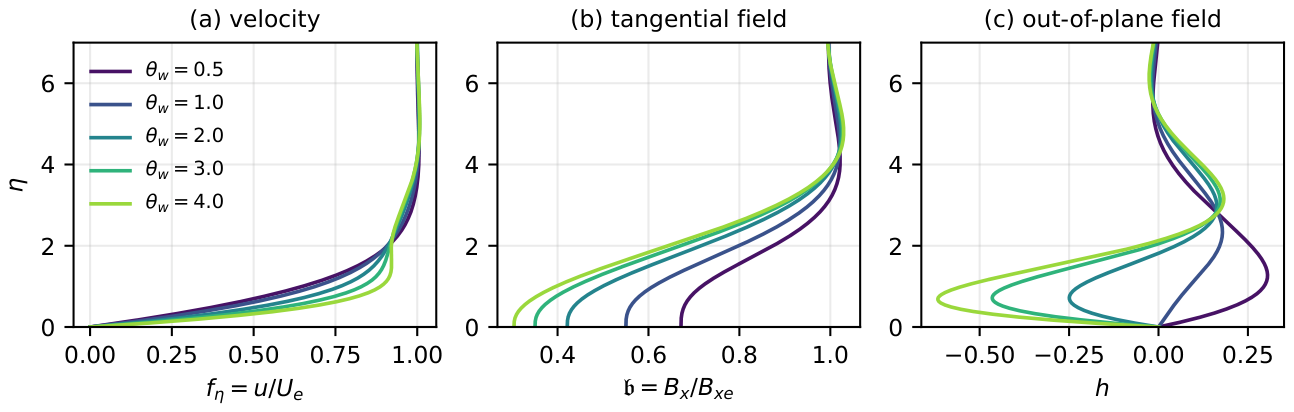
Figure 2.
(a) Out-of-plane field with (solid) and without (dashed) the Biermann source at , . (b) Peak amplitude against ; the Biermann contribution follows the predicted scaling of Eq. (50) while the Hall contribution is nearly independent of M.
Figure 2.
(a) Out-of-plane field with (solid) and without (dashed) the Biermann source at , . (b) Peak amplitude against ; the Biermann contribution follows the predicted scaling of Eq. (50) while the Hall contribution is nearly independent of M.
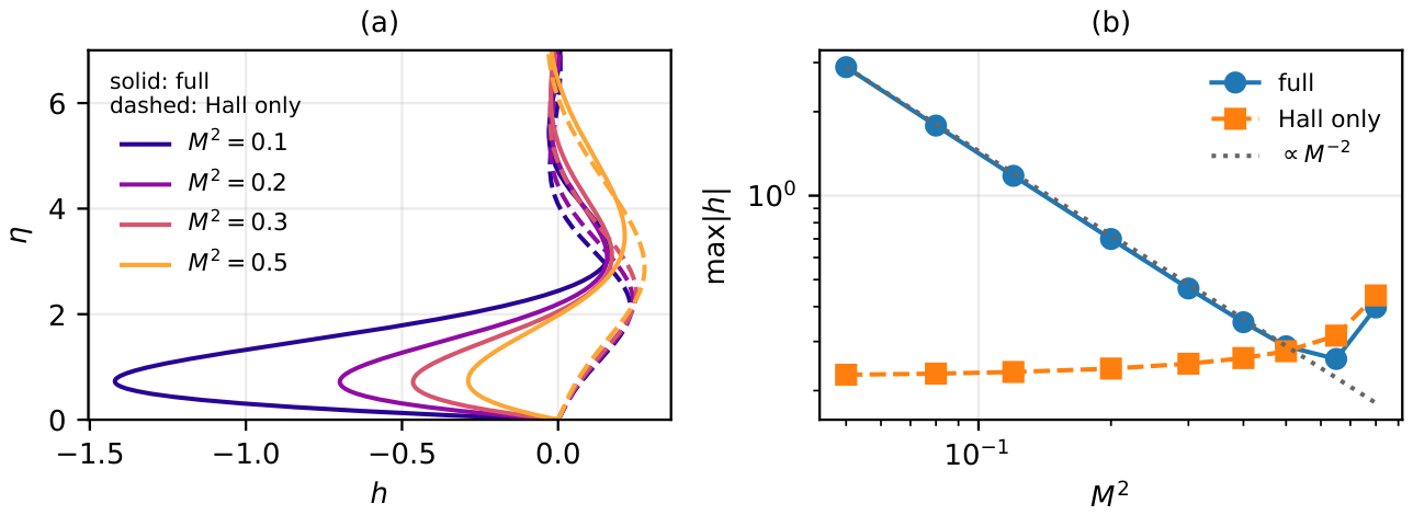
Figure 3.
(a) Wall stress against for four wall temperature ratios; all curves vanish at . (b) Back-reaction of the Hall fields on the wall stress and wall tangential field at , ; the lines have slope 2.
Figure 3.
(a) Wall stress against for four wall temperature ratios; all curves vanish at . (b) Back-reaction of the Hall fields on the wall stress and wall tangential field at , ; the lines have slope 2.
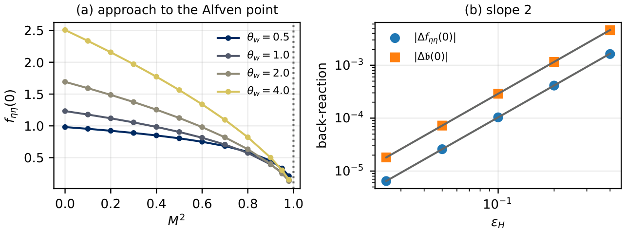
Figure 4.
Dual-temperature structure at , , , , , . (a) Ions; (b) electrons, with the free-stream value marked—note the undershoot below unity at small ; (c) the density weight that closes the reduction.
Figure 4.
Dual-temperature structure at , , , , , . (a) Ions; (b) electrons, with the free-stream value marked—note the undershoot below unity at small ; (c) the density weight that closes the reduction.
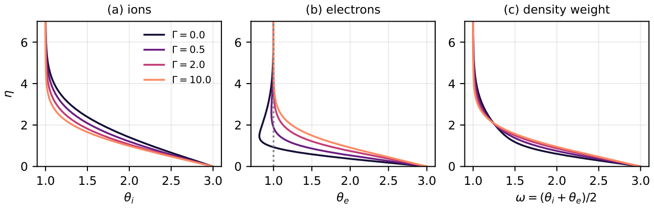
Figure 5.
Compressible flat plate with an aligned frozen-in field, adiabatic wall, , , . (a) Velocity; (b) tangential field, showing severe flux expulsion at high Mach number; (c) quadrupole.
Figure 5.
Compressible flat plate with an aligned frozen-in field, adiabatic wall, , , . (a) Velocity; (b) tangential field, showing severe flux expulsion at high Mach number; (c) quadrupole.
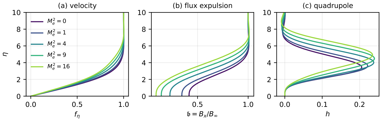

Table 1.
Validation of the two solvers against independently known results.
| Quantity | Condition | Computed | Reference |
|---|---|---|---|
| Class B, , | 1.232588 | 1.232588 (Hiemenz) | |
| Class B, , | 0.647900 | 0.647900 | |
| Class A, | 0.469600 | 0.469600 (Blasius) | |
| Class A, | 1.216781 | 1.216782 | |
| Class A, , any | 0.469600 | Mach independent | |
| r | Class A, , | 0.84771 | |
| Class B, | 0, Eq. (52) | ||
| Class A, | 0 identically | Eq. (59) | |
| back-reaction | Class B, exponent in | 2.00 | 2 |
Table 2.
Class-B steady solutions; , , , , , . is the physical-plane thickness.
| 0.50 | 0.875718 | 0.671376 | 0.87159 | 0.30480 | 1.27 | 2.6393 |
| 0.75 | 0.963786 | 0.602670 | 0.85363 | 0.21613 | 1.76 | 3.0450 |
| 1.00 | 1.050109 | 0.550179 | 0.83257 | 0.17876 | 2.34 | 3.3975 |
| 1.50 | 1.217846 | 0.474270 | 0.78672 | 0.16261 | 2.79 | 3.9985 |
| 2.00 | 1.379665 | 0.421194 | 0.73989 | 0.24948 | 0.72 | 4.5026 |
| 3.00 | 1.688367 | 0.350303 | 0.64973 | 0.46494 | 0.71 | 5.3635 |
| 4.00 | 1.980892 | 0.304031 | 0.56660 | 0.61702 | 0.69 | 6.1102 |
Table 3.
Quadrupole amplitude with and without the Biermann source; , , , .
| full | Hall only | ratio | full | |
|---|---|---|---|---|
| 0.05 | 2.89076 | 0.22802 | 12.68 | 2.06616 |
| 0.10 | 1.41986 | 0.23173 | 6.13 | 1.98936 |
| 0.20 | 0.69945 | 0.23993 | 2.92 | 1.84180 |
| 0.30 | 0.46494 | 0.24977 | 1.86 | 1.68837 |
| 0.50 | 0.28841 | 0.27684 | 1.04 | 1.35292 |
| 0.80 | 0.39734 | 0.43896 | 0.91 | 0.73012 |
Table 4.
Effect of the equipartition parameter; , , , , , . .
| 0.0 | 2.2646 | 0.9442 | 3.3666 | 0.5518 | 0.5222 |
| 0.1 | 2.2313 | 1.0651 | 3.5407 | 0.4987 | 0.5061 |
| 0.5 | 2.1500 | 1.3556 | 3.9569 | 0.3773 | 0.4696 |
| 2.0 | 2.0522 | 1.7007 | 4.4273 | 0.2591 | 0.4260 |
| 10.0 | 1.9914 | 1.9103 | 4.6844 | 0.2177 | 0.3884 |
| 50.0 | 1.9761 | 1.9599 | 4.7427 | 0.2141 | 0.3755 |
Table 5.
Class A, adiabatic wall, , , , .
| 0 | 1.000 | 0.377238 | 0.415919 | 1.00000 | 0.20567 |
| 1 | 1.333 | 0.363982 | 0.344714 | 1.22465 | 0.22160 |
| 4 | 2.333 | 0.341562 | 0.226786 | 1.84549 | 0.23777 |
| 9 | 4.000 | 0.324812 | 0.141555 | 2.79683 | 0.23955 |
| 16 | 6.333 | 0.314088 | 0.090011 | 4.04728 | 0.23457 |
Disclaimer/Publisher’s Note: The statements, opinions and data contained in all publications are solely those of the individual author(s) and contributor(s) and not of MDPI and/or the editor(s). MDPI and/or the editor(s) disclaim responsibility for any injury to people or property resulting from any ideas, methods, instructions or products referred to in the content. |
© 2026 by the authors. Licensee MDPI, Basel, Switzerland. This article is an open access article distributed under the terms and conditions of the Creative Commons Attribution (CC BY) license (http://creativecommons.org/licenses/by/4.0/).
Copyright: This open access article is published under a Creative Commons CC BY 4.0 license, which permit the free download, distribution, and reuse, provided that the author and preprint are cited in any reuse.