
Submitted:
28 August 2026
Posted:
31 August 2026
You are already at the latest version
Abstract
Ground clutter introduces stationary or recurrent nonmeteorological echoes into weather-radar remote-sensing imagery and can be difficult to remove when archived products contain reflectivity alone. This study develops an image-level ground-clutter filter using Météo-France MeteoNet radar composites from northwestern France for 2016. Candidate screening and manual interpretation produced 18 clear-air events and 34 weather events, comprising 346,629 labelled pixels; ambiguous echoes were excluded. Ten reflectivity-derived intensity, spatial, temporal, and object features were evaluated with complete events held out. A random forest (RF) achieved clutter suppression of 0.763, weather-echo preservation of 0.952, and F1=0.833, outperforming reflectivity-only deterministic rules in their balance between removal and preservation. Component size and reflectivity were the leading permutation-importance variables, while temporal statistics provided a smaller complementary contribution. Rain-gauge data were used only for period screening, recurrent-clutter station confirmation, and an auxiliary downstream check. At nine confirmed stations, 4014 paired 30-min samples showed that RF gating reduced mean absolute error from 0.055 to 0.052 mm and false-alarm ratio from 0.277 to 0.181; root-mean-square error remained essentially unchanged (0.283 to 0.284 mm), while probability of detection increased from 0.635 to 0.738 and the critical success index increased from 0.511 to 0.635. These results show that the proposed reflectivity-only RF filter removes recurrent ground clutter while retaining most weather echoes, and the independent gauge comparison further shows that targeted filtering reduces false precipitation detections at confirmed clutter sites.
Keywords:
weather radar
; remote sensing
; ground clutter
; manual annotation
; random forest
1. Introduction
Weather radar is an active microwave remote-sensing system that repeatedly maps atmospheric backscatter over large areas [1,2]. In an image sequence, reflectivity intensity, neighborhood texture, echo geometry, and temporal evolution jointly describe meteorological structures. These spatially continuous observations underpin precipitation monitoring, hydrological forecasting, numerical-weather-prediction assimilation, and severe-weather surveillance [3,4]. Reliable interpretation begins with quality control: calibration, sampling geometry, beam blockage, attenuation, vertical reflectivity structure, and nonmeteorological contamination can all propagate into derived radar products [5,6,7].
Ground clutter is a central quality-control problem because terrain, buildings, vegetation, infrastructure, and other stationary or slowly varying targets can return energy to the radar. Under normal propagation it often recurs near fixed locations; anomalous refractive conditions can extend contamination into regions that are normally clear. Such echoes can obscure precipitation, distort spatial morphology, and appear as false light rainfall after reflectivity is converted to rain rate. Their expression also varies with scan geometry, propagation, composite processing, and nearby meteorological echo, so a fixed reflectivity threshold alone cannot reliably separate clutter from precipitation [8,9,10].
The available variables determine the appropriate filtering strategy. At signal level, Doppler spectra support suppression of power near zero radial velocity and reconstruction of weather moments [11,12,13,14]. Polarimetric systems additionally exploit differential and correlation variables to distinguish precipitation from biological, propagation, and surface returns [15,16,17]. Historical mosaics and many distributed products, however, preserve only gridded reflectivity. For these archives, clutter filtering must operate on image evidence such as local variability, vertical or horizontal continuity, echo extent, recurrence, and motion [10,18,19].
Reflectivity-only filtering presents two linked methodological challenges. First, weak precipitation and ground clutter can overlap in reflectivity magnitude, while mixed pixels and anomalous propagation may blur their spatial signatures. Time-ordered imagery offers additional evidence because persistent compact structures differ from coherently evolving weather echoes, but temporal persistence must complement rather than replace spatial context. Second, neighboring pixels and consecutive scans are strongly dependent. Random pixel or window splits can therefore place nearly identical structures in both training and validation data and inflate apparent generalization. Complete-event separation is required to evaluate transfer to unseen echo situations.
This study addresses ground-clutter filtering as the primary remote-sensing task. Pixel classes are assigned manually from the radar fields and their full 30-min temporal context, and the classifier uses only reflectivity-derived image features. Rain gauges have separate supporting roles: they screen candidate periods, help identify stations affected by recurrent dry-weather echoes, and provide an auxiliary paired check of the filtered product. They are neither pixel labels nor deployment-time classifier inputs. The objectives are to:
- 1.
- construct a consistently annotated pixel dataset of ground clutter and weather echoes from screened radar periods;
- 2.
- compare learned classifiers with reflectivity-only local-density, temporal-persistence, and spatiotemporal rule baselines under identical out-of-event validation;
- 3.
- quantify the contribution of spatial and temporal reflectivity-image features;
- 4.
- use paired 30-min gauge comparisons as an auxiliary test of how clutter filtering changes false rainfall and precipitation preservation at recurrent-clutter stations.
The main contribution is an event-aware, reflectivity-only filtering framework that links manual annotation, image-derived classification, complete-event validation, and recurrent-clutter screening. The downstream gauge analysis is deliberately secondary: it tests whether radar-domain suppression translates into fewer false precipitation detections without redefining the study as a QPE method.
2. Related Work
2.1. Signal-Level Ground-Clutter Suppression
Signal-level filters exploit the concentration of stationary-clutter power near zero radial velocity or model the Doppler spectrum directly. GMAP identifies a clutter-contaminated spectral interval, removes it, and reconstructs the weather spectrum; later adaptive, regression, and object-oriented methods refine spectral identification and weather-moment recovery [11,12,13,14,20,21,22]. This approach is physically close to the clutter-generation mechanism and can preserve meteorological power when the clutter and weather spectra are separable.
Spectral overlap remains difficult when weather echoes also occupy near-zero radial velocity, and excessive filtering can bias precipitation estimates [13]. More fundamentally for remote-sensing archives, signal-level processing requires complex time series or spectral moments at the radar gate. Once measurements have been resampled into a reflectivity-only composite, those observables cannot be reconstructed from the image. Image-level filtering is therefore not a replacement for spectral processing at the radar, but a necessary quality-control layer for products in which signal information is no longer available.
2.2. Reflectivity-Structure and Learning-Based Classification
Product-level methods infer echo type from the organization of radar fields. Three-dimensional reflectivity structure has been used to identify nonprecipitating echo from vertical extent, spatial variability, and vertical intensity gradients [18]. For two-dimensional products, local texture, gradients, echo continuity, and neighboring-pixel statistics supply related contextual evidence. Neural-network and fuzzy-logic classifiers established that reflectivity structure can distinguish anomalous-propagation or nonprecipitating echo even when the separation is not represented by one hard threshold [8,9].
More broadly, data-driven models have demonstrated effective representation learning and sequential decision optimization in heterogeneous aerial and space–air–ground systems, including deep traffic classification, computation offloading, and LEO-satellite handover [23,24,25]. These studies provide methodological context for learning from complex, coupled observations, but they do not constitute direct radar-clutter baselines. Given the moderate number of independent annotated events and the need for interpretable feature attribution, the present study therefore uses tree ensembles rather than a deep or reinforcement-learning architecture.
Operational reflectivity quality control combines several indicators so that isolated intensity, texture, and continuity failures do not dominate the decision [6,10]. Sequence models extend the feature space from one scan to coherent evolution across scans, while recurrence maps summarize repeated contamination at fixed locations [19,26]. These studies motivate the present combination of central reflectivity, local neighborhood statistics, connected-object extent, and short-term temporal descriptors. Manual annotation remains important because the target distinction is visual and contextual: stationary clutter embedded near precipitation should not be inferred solely from an automatic proxy.
2.3. Polarimetric and Operational Quality Control
Dual-polarization radar provides additional physical separation through correlation coefficient, differential reflectivity, differential phase, velocity, and spectrum width. Fuzzy-logic and physically based classifiers combine these measurements with texture and environmental context to identify meteorological and nonmeteorological echo [15,16,17,27]. Such systems show the benefit of multi-source quality indices and of retaining graded confidence rather than relying only on binary removal.
Operational monitoring also emphasizes the effect of quality control on downstream radar products. A filter that maximizes clutter removal can still damage weak or slow-moving precipitation, so echo suppression and meteorological-echo preservation must be reported together [7,28]. This principle is carried into the present reflectivity-only setting through a primary radar-domain evaluation against manual labels and a separate gauge-based occurrence check.
2.4. Validation Gap in Reflectivity-Only Archives
Many learning-based echo classifiers are evaluated with randomly selected gates, pixels, or scans. In a radar-image sequence, however, adjacent samples share storm morphology, clutter locations, and acquisition conditions. Evaluation on complete withheld events is the more direct test of whether a model transfers to a new episode rather than recognizing structures already represented in training. It also exposes the difference between pooled pixel performance and between-event stability.
The remaining validation need is to connect classification with controlled application. This study therefore evaluates suppression and weather-echo preservation against manual pixel labels, compares learned and deterministic reflectivity-only filters on the same event folds, and confirms recurrent clutter independently at station locations. Paired 30-min gauge comparisons are then used only as an auxiliary consequence check. This hierarchy keeps the scientific claim centred on ground-clutter filtering while showing how the filtering decision affects false precipitation detections in an external observation stream.
3. Materials and Methods
3.1. Radar-Image–Gauge Observation Integration
Figure 1 summarizes the observational design in four stages. Stage A separates the radar-image and gauge-observation streams. Stage B derives spatial–temporal reflectivity predictors and records manually assigned pixel classes within screened windows. Stage C performs complete-event validation and feature ablation for random forest (RF) and gradient-boosted decision tree (GBDT) classifiers. Stage D applies the nine-feature gate before an auxiliary paired station–time QPE check. Dashed links indicate where gauge observations support candidate-period screening and downstream verification; gauge values are not classifier predictors.
The framework uses observation-level coordination: the deployable classifier is driven by radar-image features, while gauges provide independent evidence for candidate-period selection, station screening, and paired QPE evaluation. The two data streams meet at the validation stage, preserving a clear correspondence among pixel prediction, station confirmation, and quantitative assessment.
3.2. Reflectivity Features and Classifiers
Ten features were computed from the radar remote-sensing imagery for the central scan of each 30-min window (Table 1). Spatial features summarize a neighborhood. Temporal features summarize all scans in the window. Connected-component size describes the extent of the central-scan echo object. No gauge variable was included in this pixel-level predictor vector; gauge information entered through candidate-period screening and the independent evaluation pathways shown in Figure 1.
Figure 2 shows how the scan window, local patch, temporal trajectory, and connected echo object are converted into model inputs. The diagram also makes the separation between the primary classification experiment and auxiliary downstream verification explicit: the classifier produces a ground-clutter probability, the fixed gate changes only predicted pixels, and raw and filtered QPE are compared on the same station–time samples.
3.3. Station Screening for Targeted QPE
The 76 reliable no-rain windows were consolidated into 18 clear-air events for radar-domain recurrence analysis. A wider set of 301 station-supported no-rain windows was independently merged into 36 dry episodes for station screening. Twenty-six episodes were used to establish the station groups. A station was considered to contain a dry echo in an episode when the maximum reflectivity in its nearest neighborhood was at least 8 dBZ.
Candidate recurrent-echo stations were required to lie in the highest 20% of nonzero calibration-event echo frequencies and to contain echoes in at least three calibration episodes. Clean stations contained no such echo in any calibration episode; remaining stations formed a boundary group. The procedure yielded 10 recurrent-echo candidates, 176 clean stations, and 64 boundary stations. Review across multiple dry events confirmed recurrent ground clutter at all 10 candidates. This station confirmation was performed separately from the manual pixel annotation used to train the classifiers.
3.4. Auxiliary Paired 30-min QPE Check
The QPE gate used nine of the ten image features: central reflectivity, the four local-neighborhood statistics, and the four temporal statistics. Connected-component size was omitted because computing it would require the complete image rather than the station-centred patch. Before QPE application, this exact nine-feature RF was evaluated using the same four out-of-event folds, fixed hyperparameters, class-balanced sample weights, and probability threshold of 0.5 used in the main RF analysis. After the out-of-fold predictions had been recorded, one final model was fitted to all 346,629 manually annotated pixels. No QPE event was used for classifier fitting, hyperparameter selection, or threshold selection.
The auxiliary QPE check used 20 rain episodes and the 10 held-out dry episodes. Evaluation periods were at least 2 h away from every annotation window. The final set contained 104,915 complete 30-min station–time samples from 237 stations; nine of the 10 manually confirmed stations met all radar and gauge completeness requirements.
Both raw and filtered QPE used identical samples and the Marshall–Palmer relation [29]
where Z is linear reflectivity and R is rain rate. At each 5-min scan, the nine features were calculated from the station cell, its neighborhood, and all scans in the corresponding 30-min window. The fitted RF returned the probability of the manually annotated ground-clutter class. Valid station-cell echoes at or above 8 dBZ with probability were set to zero before 30-min integration; all other valid echoes were retained. Radar rain rate was averaged across the valid scans and multiplied by 0.5 h. Gauge observations were summed in the identical 30-min bin, which was retained when at least four gauge records and the radar estimates were valid.
For the auxiliary check, targeted RF applied the gate only at the manually confirmed recurrent-clutter stations and left all other stations unchanged. This policy isolates the downstream effect at locations where repeated dry-weather radar evidence supports application of the clutter filter.
4. Experimental Results and Discussion
This section follows the hierarchy of the experimental evidence. Section 4.1 specifies the study area and observations, data preparation, evaluation metrics and baselines, and implementation details. Section 4.2 first reports radar-domain classification and qualitative clutter-filtering behaviour, then uses paired QPE only as an auxiliary downstream check.
4.1. Experiment Settings
4.1.1. Study Area and Observations
Radar and gauge observations were obtained from MeteoNet, an open meteorological dataset released by Météo-France under the Etalab Open Licence 2.0 [30]. MeteoNet covers northwestern (NW) and southeastern France for 2016–2018; this study used the NW 2016 old-reflectivity archive and the corresponding NW ground-station archive. The exact public source archives are listed in the Data Availability Statement.
The official radar documentation specifies one .npz archive record per 10- or 11-day period, with arrays for radar maps, scan times, and missing scan times [31]. Successive fields are nominally separated by 5 min, the angular grid spacing is , and coordinates use WGS 84 geographic latitude and longitude (EPSG:4326). The selected 2016 archive records contain 26,199 scans, with nine nominal scans listed as missing. Each field has cells spanning approximately – N and W– E. The old product stores the lower bound of discretized reflectivity intervals in decibels of reflectivity (dBZ): values below 8 dBZ are coded as 0, the first detected interval is stored as 8 dBZ, and code 255 represents missing data. Consequently, 8 dBZ is both the product’s lowest resolved echo level and the basic echo threshold adopted in this study.
MeteoNet ground observations are reported nominally every 6 min and include station identifier, coordinates, altitude, precipitation, relative humidity, temperature, dew-point temperature, wind, and sea-level pressure [32]. The corresponding selected 2016 records in NW2016.csv contain 1,201,215 raw observations from 285 unique station coordinates. After domain matching and experiment-specific completeness screening, 250 stations were available for clear-air station screening and 237 for the final paired QPE analysis. Gauge coordinates were mapped to the nearest radar-cell centre using great-circle distance, and the final QPE analysis retained only station–radar matches within 25 km.
Following the public product definition, the input was treated consistently as a WGS 84 gridded composite-reflectivity product, with quality control and feature computation based on its documented time step, grid, reflectivity coding, and missing-value rules.
4.1.2. Data Pre-Processing and Analysis
Gauge observations were aggregated into 30-min windows. A candidate no-rain window was required to have zero reported precipitation throughout the target window and a buffer extending one hour before and after it, at least 935 valid precipitation records per 30-min bin across the domain, median relative humidity no greater than 90%, 90th-percentile relative humidity no greater than 99%, and median dew-point depression of at least 1 °C. These criteria exclude widespread precipitation and near-saturated boundary-layer conditions but do not constitute a conventional cloud observation.
A radar window entered the clear-air annotation pool when it contained at least five scans, echoes were defined at dBZ, at least 30% of the union echo area persisted in two-thirds of the scans, the median Jaccard overlap of adjacent echo masks was at least 0.40, and mean echo coverage was between 0.002% and 35%. Seventy-six 30-min windows satisfied all criteria.
Rainy annotation windows were selected independently from periods with at least 100 rainy gauge records, at least 900 valid precipitation observations, and positive domain-total precipitation. Candidate weather-echo pixels had reflectivity of at least 12 dBZ, local echo density of at least 0.35, temporal echo presence of at least 0.33, and a connected component of at least 80 pixels. These criteria reduced the volume presented for review; they did not determine the final class.
Each candidate was manually annotated using its central scan, local spatial context, and complete 30-min sequence, with three possible outcomes: ground clutter, weather echo, or ambiguous. Ground clutter was identified by a fixed or recurrent localized structure that did not move with the surrounding precipitation field; weather echo was identified by spatial continuity and coherent displacement or evolution; ambiguous cases, including overlap between precipitation and stationary echo, were excluded. Annotation masks yielded 142,629 ground-clutter pixels and 204,000 weather-echo pixels (346,629 labelled pixels in total). One protocol, fixed class definitions, and the same temporal context were used throughout.
Consecutive annotated windows of the same class were merged when their time separation did not exceed 2 h. This produced 18 clear-air events and 34 weather-echo events. A wider set of 301 station-supported no-rain windows was independently merged into 36 dry events for station screening, while the QPE experiment used 20 rain events and 10 held-out dry events.
4.1.3. Evaluation Metrics and Baseline Methods
For classifier validation, the positive class is manually annotated ground clutter. Reported metrics include precision, clutter-suppression rate (positive-class recall), weather-echo preservation (specificity), critical success index (CSI), F1, Matthews correlation coefficient (MCC), receiver-operating-characteristic area under the curve (ROC-AUC), and precision–recall area under the curve (PR-AUC).
QPE was evaluated using mean absolute error (MAE), root-mean-square error (RMSE), mean bias error, relative bias, correlation, , probability of detection (POD), false-alarm ratio (FAR), and CSI. Rain occurrence used a common 0.1-mm threshold for each 30-min accumulation, equivalent to an intensity threshold of 0.2 mm h−1. With prediction and gauge value ,
Three deterministic baselines were defined using only reflectivity features available to the station-centred QPE gate. The local-density rule classified an echo as clutter when its echo density was below a threshold. Candidate values were 0.08, 0.12, 0.18, 0.25, 0.35, and 0.50. The temporal-persistence rule required temporal presence to exceed 0.50, 0.67, 0.83, or 0.99; temporal standard deviation to be no greater than 2, 4, 6, 8, or 12 dBZ; and mean absolute scan-to-scan change to be no greater than 2, 4, 6, or 10 dBZ. The spatiotemporal rule used either the intersection or union of the two component decisions.
The baseline comparison used the same held-out events, annotated pixels, and event-stratified bootstrap as the learned models. Rule parameters and combination logic were selected only within the corresponding outer training folds by maximizing training-event F1, with weather-echo preservation used to break ties. This design prevents the baseline comparison from using the outer test events for parameter selection.
4.1.4. Implementation Details
Two ensemble classifiers implemented in scikit-learn [33] were compared. The RF used 180 trees, maximum depth 16, minimum leaf size 8, square-root feature subsampling, balanced bootstrap class weights, and random seed 42. The histogram GBDT used 180 iterations, learning rate 0.07, at most 31 leaves, minimum leaf size 30, and regularization 0.2. The probability threshold was fixed at 0.5 for all out-of-event predictions.
Four outer folds were defined by assigning complete clear-air and weather events with monthly balancing. No pixel or window from a withheld event entered training for that fold. Five variants were evaluated from concatenated out-of-fold predictions: RF with all features, GBDT with all features, RF without temporal features, RF without spatial features, and RF with instantaneous reflectivity only. Classifier confidence intervals were calculated from 5000 event-stratified bootstrap replicates, resampling complete clear-air and weather-echo events separately.
After out-of-fold predictions had been recorded, one final nine-feature RF was fitted to all 346,629 annotated pixels for the independent QPE experiment. Final rule parameters were likewise selected from the complete annotated dataset: a local-density threshold of 0.50, temporal presence of at least 0.50, temporal standard deviation no greater than 6 dBZ, mean absolute change no greater than 10 dBZ, and the union of the local-density and temporal decisions. The QPE episodes were not used to fit the RF or choose these parameters.
Four representative out-of-event clear-air scenes, one from each outer fold, were retained as qualitative comparisons. For each scene, RF and GBDT were refitted after excluding its complete outer fold, and rule parameters were selected from the same outer training fold. Retained fraction is defined as the number of valid central-scan echo pixels at or above 8 dBZ after filtering divided by the corresponding raw count; it measures filter aggressiveness rather than classification accuracy.
For the auxiliary QPE check, raw and filtered scores were calculated on identical 30-min station–time samples so that changes followed only from the filtering decision. With these settings fixed, the following section reports radar-domain classification first, followed by qualitative cases, the auxiliary paired check, and their integrated interpretation.
4.2. Results and Discussion
4.2.1. Radar-Domain Recurrence and Classification
The 76 reliable no-rain windows were consolidated into 18 independent clear-air events, and 34 rainy windows formed 34 weather events. Consolidation prevented adjacent windows from the same continuous process from being treated as independent samples. Manual annotation then produced 142,629 ground-clutter pixels and 204,000 weather-echo pixels, with ambiguous pixels excluded as described in Section 4.1.2.
Figure 3a locates the study area in western Europe and gives the exact radar-composite extent; Figure 3b,c shows the recurrent clear-air echo structure at two thresholds. At 10 dBZ, pixels recurring across at least half of the clear-air events were sparse and did not overlap a gauge. At 5 dBZ, recurrent areas expanded, while the nearest recurrent area remained 33.1 km from a gauge. The regional recurrence map therefore supports stable-structure case selection, and station groups are subsequently determined by the dry-event screening procedure in Section 3.3.
Using the manually annotated classes, Table 2 reports pooled metrics from four-fold out-of-event predictions. The full-feature RF achieved clutter suppression of 0.763, weather-echo preservation of 0.952, F1 of 0.833, and MCC of 0.742. The full gradient-boosting model produced similar F1 (0.828) but slightly lower weather-echo preservation (0.934). Event-to-event differences in echo structure and clutter intensity produced a clutter-suppression 95% interval of 0.491–0.956, while weather-echo preservation was more stable at 0.930–0.971.
The rule baselines exposed two contrasting operating regimes. The local-density rule preserved 0.998 of weather echoes but suppressed 0.068 of clutter. The temporal-persistence and spatiotemporal rules increased clutter suppression to 0.786 and 0.826, respectively, while preserving 0.417 and 0.415 of weather echoes. Their F1 scores were 0.600 and 0.620. The RF provided the most balanced pooled estimate, with F1=0.833, clutter suppression of 0.763, and weather-echo preservation of 0.952. The comparison is interpreted through this joint operating balance rather than through a single pairwise interval.
A non-grouped window-level analysis yielded RF F1=0.975, whereas event-grouped out-of-fold validation yielded 0.833. Because the threshold and split design also differed, the 0.142 decrease is diagnostic rather than a single-factor causal estimate. In this experiment, the window-level score therefore overestimated performance on complete withheld events.
Feature ablation in Table 2 and Figure 4 further separates the roles of the predictor groups. Removing temporal features reduced RF F1 by only 0.008, indicating that temporal statistics supplied a modest complementary contribution rather than driving the classifier.
Removing spatial features increased clutter recall from 0.763 to 0.872 but reduced weather-echo preservation from 0.952 to 0.862. Thus, spatial context mainly controlled false removal of coherent weather echoes rather than maximizing clutter recall. Instantaneous reflectivity alone achieved F1=0.817, but its lower PR-AUC (0.917) and preservation (0.930) indicate that contextual features improved discrimination. Together, the ablations show that spatial structure constrains echo morphology, while temporal statistics provide complementary persistence information.
The normalized out-of-fold confusion matrix in Figure 5a shows that the full RF retained 95.2% of manually annotated weather-echo pixels and identified 76.3% of manually annotated ground-clutter pixels. Event-fold permutation importance (Figure 5b) was calculated by permuting one feature at a time within each held-out fold and measuring the decrease in balanced accuracy. Open circles retain the fold-level values, while the mean diamond and full fold range provide a compact view of both ranking and variability. Component size produced the largest mean decrease (0.116), followed by reflectivity (0.071), local maximum (0.021), and temporal mean (0.014). These values describe predictive dependence rather than physical causality.
Because the station-centred QPE implementation omits connected-component size, its exact nine-feature RF was validated separately before downstream application. It achieved out-of-event clutter suppression of 0.868 (95% event-bootstrap CI: 0.780–0.947), weather-echo preservation of 0.881 (0.844–0.911), and F1=0.852 (0.761–0.917) against the manual annotations. These predictions were generated before the final nine-feature RF was refitted on all annotated pixels. The 30 QPE evaluation episodes remained separated from every annotation window and were not used to fit the classifier, tune hyperparameters, or select the probability threshold.
4.2.2. Qualitative Filtering Comparisons
Figure 6, Figure 7, Figure 8 and Figure 9 show four representative clear-air scenes, one from each outer fold. Each six-panel comparison uses a common crop and reflectivity scale and includes the raw field, the local-density and temporal-persistence rules, both learned classifiers, and the pure spatiotemporal rule. For each scene, the displayed RF and GBDT predictions were generated by models trained without the complete outer fold containing that scene; the rule parameters were also selected without that fold.
The local-density rule retained 91.8–97.1% of the raw echo pixels. The temporal-persistence rule retained 12.6–38.1%. The learned filters varied more strongly across events. RF retained 13.6% on 6 May, 91.8% on 8 May, 3.7% on 24 May, and 26.2% on 3 November; the corresponding GBDT fractions were 14.0%, 42.8%, 21.6%, and 41.4%. The spatiotemporal rule retained 10.9–33.2%. These scene-level fractions are consistent with the quantitative comparison: the local-density rule was conservative, whereas temporal persistence and its union with the density decision removed substantially more echo.
The displayed structures are examples from the clear-air events used in the annotation study. Retained fractions quantify filter aggressiveness only; the event-grouped metrics against held-out manual labels and the paired gauge analysis provide the quantitative evidence for classification and downstream effects.
4.2.3. Auxiliary Paired QPE Check
With the confirmed-station set fixed, Table 3 compares raw and targeted-RF 30-min QPE on identical station–time samples. At the nine manually confirmed recurrent-clutter stations, MAE decreased from 0.055 to 0.052 mm and FAR from 0.277 to 0.181; RMSE changed by less than 0.001 mm, while POD increased from 0.635 to 0.738. From the reported POD and FAR, CSI was calculated as 0.635, compared with 0.511 for the raw field. The confirmed-station comparison therefore shows simultaneous reductions in false alarms and improvements in precipitation detection, while remaining auxiliary evidence for the radar-domain filter rather than the basis of the primary classification claim.
At confirmed stations, FAR decreased by 0.096, POD increased by 0.103, and CSI increased by 0.124. The approximately 0.0024-mm MAE decrease was modest and RMSE was effectively unchanged. The continuous and categorical scores therefore describe a reduction in recurrent false echo together with improved rain-occurrence discrimination.
Targeted RF produced these confirmed-station changes while leaving clean and boundary stations unchanged by design. Spatial targeting therefore concentrates the intervention at locations with the clearest recurrent-clutter signature and avoids unnecessary modification elsewhere in the domain.
The preceding analyses represent connected levels of evidence. Event-grouped classification quantifies discrimination against manual pixel labels, station screening identifies where the gate is applied, and the auxiliary paired QPE check measures the downstream balance between false-alarm reduction and precipitation preservation. Their joint interpretation is more informative than any single metric: stronger clutter suppression does not necessarily imply better precipitation estimation.
4.2.4. Integrated Interpretation
Taken together, the results support three conclusions about reflectivity-only ground-clutter filtering. First, image-derived reflectivity magnitude, local texture, echo extent, and short-term persistence discriminate manually annotated ground clutter from weather echoes across withheld events. The event-grouped RF F1 of 0.833 provides the relevant estimate because complete events were held out; the non-grouped window-level value was 0.975. The best rule-based F1 was 0.620. The rule comparison further shows why clutter suppression alone is insufficient: the spatiotemporal rule suppressed 0.826 of clutter but preserved only 0.415 of weather echoes. Second, station screening identifies recurrent dry-weather echoes and supplies a spatial gate for applying the classifier. Third, the auxiliary gauge check shows that filtering reduces false alarms and improves POD and CSI at confirmed sites, while targeted application leaves other station groups unchanged.
These findings are consistent with earlier reflectivity-context methods that combine local statistics and object continuity [10], with operational systems that combine several quality indicators [6], and with persistent-clutter probability maps derived from repeated observations [26]. The present contribution links manually annotated reflectivity-only mosaics to gauge-assisted period selection, station screening, and a downstream paired occurrence check. Gauges provide independent precipitation evidence: they constrain the periods entering annotation and station confirmation and expose the false-alarm–miss balance after filtering.
4.2.5. False-Alarm Reduction and Precipitation Preservation
Quality control is not optimal merely because it removes many non-meteorological echoes. Hubbert et al. showed that indiscriminate clutter filtering can bias weather returns near zero velocity [13]; product-level classification has the analogous risk of removing weak or spatially fragmented precipitation. Continental-scale monitoring has similarly emphasized independent occurrence verification when introducing quality-control changes [7].
The 30-min paired check quantifies the downstream effect. At confirmed recurrent-clutter stations, RF gating reduced FAR from 0.277 to 0.181 and MAE from 0.055 to 0.052 mm, increased POD from 0.635 to 0.738 and CSI from 0.511 to 0.635, and left RMSE essentially unchanged. Targeting the gate leaves all other station estimates unchanged, so the radar-domain classifier can suppress recurrent contamination without modifying the full station network.
Spatial targeting is therefore the recommended implementation. Applying the gate at confirmed recurrent-clutter stations preserves the original estimates elsewhere. The screening list can be updated with radar calibration, surroundings, propagation conditions, and mosaic processing, while a probability-to-quality-index mapping can further provide continuous rather than binary control.
4.2.6. Comparison with Polarimetric and Signal-Level Approaches
Polarimetric classifiers use correlation coefficient, differential reflectivity, differential phase, Doppler velocity, and spectrum width for physically informed echo classification [15,17,27,34]. Signal-level methods process near-zero-frequency spectral components and reconstruct weather moments [11,14]. The present approach operates at the reflectivity-image level: it learns ground-clutter probability from intensity, texture, object extent, and temporal persistence, then applies the resulting decision directly to archived image fields. Signal-, polarimetric-, and image-level methods consequently address complementary stages of radar quality control.
4.2.7. Implementation and Quality Control
Four consistency controls structure the complete workflow. First, all training and validation pixels are manually annotated under one spatial–temporal protocol, with mixed or ambiguous pixels excluded from model fitting. Second, model selection and performance estimation use complete-event folds, preventing adjacent scans from sharing a weather situation across training and validation. Third, calibration dry events identify stations with recurrent clutter and direct spatially targeted gating to those locations. Finally, auxiliary raw and filtered QPE use identical 30-min station–time samples. Pixel classification, station screening, and gauge comparison therefore retain distinct, sequential roles.
5. Conclusion
An event-grouped framework was developed for filtering ground clutter in reflectivity-only weather-radar remote-sensing imagery. Ten image-derived intensity, spatial, temporal, and object features enabled RF and gradient-boosting models to distinguish manually annotated ground-clutter and weather-echo pixels across withheld events. The full RF achieved event-grouped F1=0.833, clutter suppression=0.763, and weather-echo preservation=0.952. Consolidating the annotated windows into 18 clear-air and 34 weather events prevented adjacent windows from being treated as independent observations. Component size and reflectivity carried the greatest predictive importance, spatial context protected coherent weather echo, and temporal features supplied a modest complementary contribution.
The evidence sources retained distinct roles: radar imagery supplied the predictors and filtered field, and manual annotation supplied the pixel classes. Gauges supported candidate-period screening, recurrent-clutter station confirmation, and auxiliary paired verification; they did not define the pixel labels or enter the classifier. At nine confirmed stations, the 30-min check showed a FAR reduction from 0.277 to 0.181 and an MAE reduction from 0.055 to 0.052 mm. RMSE was essentially unchanged, while POD increased from 0.635 to 0.738 and CSI increased from 0.511 to 0.635, supporting the effectiveness of the targeted clutter-filtering strategy.
The central contribution is therefore the remote-sensing clutter filter and its event-level validation, not a new QPE algorithm. The exact nine-feature gate used in the auxiliary check was validated on complete held-out annotation events before final refitting, and the gauge-check events were excluded from training and tuning. Manual labels, complete-event folds, explicit weather-echo preservation, and spatially targeted application provide a coherent basis for filtering recurrent ground clutter from reflectivity-only radar archives.
Author Contributions
Conceptualization, W.Q. and C.C.; methodology, W.Q. and C.C.; software, W.Q. and Y.B.; validation, W.Q., Y.Z. and Q.D.; formal analysis, W.Q. and S.W.; investigation, W.Q. and Y.B.; resources, C.C. and Y.Z.; data curation, W.Q. and Q.D.; writing—original draft preparation, W.Q.; writing—review and editing, C.C., Y.Z., Y.B., Q.D. and S.W.; visualization, W.Q. and Y.B.; supervision, C.C.; project administration, C.C. and Y.Z.; funding acquisition, C.C. All authors have read and agreed to the published version of the manuscript.
Funding
This work was supported by the National Key Research and Development Program of China (2025YFF0514800), the Xidian–UTAR China–Malaysia Science and Technology Institute under the Fundamental Research Funds for the Central Universities (XURF-2026-QTZX26085), and the Proof-of-Concept Fund of the Hangzhou Research Institute of Xidian University (GNYZ2023QC0201, GNYZ2024QC004, and GNYZ2024QC015).
Institutional Review Board Statement
Not applicable.
Informed Consent Statement
Not applicable.
Data Availability Statement
The original data are publicly available from Météo-France’s MeteoNet repository under the Etalab Open Licence 2.0. The NW 2016 old-reflectivity archive is available at https://meteonet.umr-cnrm.fr/dataset/data/NW/radar/reflectivity_old_product/NW_reflectivity_old_product_2016.tar.gz, and the corresponding ground-station archive is available at https://meteonet.umr-cnrm.fr/dataset/data/NW/ground_stations/NW_ground_stations_2016.tar.gz (both accessed on 31 July 2026). The derived manual annotations, analysis outputs, and code are available from the corresponding author upon reasonable request.
Conflicts of Interest
The authors declare no conflict of interest.
References
- Bringi, V.N.; Chandrasekar, V. Polarimetric Doppler Weather Radar: Principles and Applications; Cambridge University Press: Cambridge, UK, 2001. [Google Scholar] [CrossRef]
- Ryzhkov, A.V.; Zrnić, D.S. Radar Polarimetry for Weather Observations; Springer: Cham, Switzerland, 2019. [Google Scholar] [CrossRef]
- Zhang, J.; Howard, K.; Langston, C.; Kaney, B.; Qi, Y.; Tang, L.; Grams, H.; Wang, Y.; Cocks, S.; Martinaitis, S.; et al. Multi-Radar Multi-Sensor (MRMS) Quantitative Precipitation Estimation: Initial Operating Capabilities. Bull. Am. Meteorol. Soc. 2016, 97, 621–638. [Google Scholar] [CrossRef]
- Ryzhkov, A.; Zhang, P.; Bukovčić, P.; Zhang, J.; Cocks, S. Polarimetric Radar Quantitative Precipitation Estimation. Remote Sens. 2022, 14, 1695. [Google Scholar] [CrossRef]
- Harrison, D.L.; Driscoll, S.J.; Kitchen, M. Improving Precipitation Estimates from Weather Radar Using Quality Control and Correction Techniques. Meteorol. Appl. 2000, 7, 135–144. [Google Scholar] [CrossRef]
- Ośródka, K.; Szturc, J. Improvement in Algorithms for Quality Control of Weather Radar Data (RADVOL-QC System). Atmos. Meas. Tech. 2022, 15, 261–277. [Google Scholar] [CrossRef]
- Michelson, D.; Hansen, B.; Jacques, D.; Lemay, F.; Rodriguez, P. Monitoring the Impacts of Weather Radar Data Quality Control for Quantitative Application at the Continental Scale. Meteorol. Appl. 2020, 27, e1929. [Google Scholar] [CrossRef]
- Grecu, M.; Krajewski, W.F. An Efficient Methodology for Detection of Anomalous Propagation Echoes in Radar Reflectivity Data Using Neural Networks. J. Atmos. Ocean. Technol. 2000, 17, 121–129. [Google Scholar] [CrossRef]
- Berenguer, M.; Sempere-Torres, D.; Corral, C.; Sánchez-Diezma, R. A Fuzzy Logic Technique for Identifying Nonprecipitating Echoes in Radar Scans. J. Atmos. Ocean. Technol. 2006, 23, 1157–1180. [Google Scholar] [CrossRef]
- Lakshmanan, V.; Fritz, A.; Smith, T.; Hondl, K.; Stumpf, G.J. An Automated Technique to Quality Control Radar Reflectivity Data. J. Appl. Meteorol. Climatol. 2007, 46, 288–305. [Google Scholar] [CrossRef]
- Siggia, A.D.; Passarelli, R.E. Gaussian Model Adaptive Processing (GMAP) for Improved Ground Clutter Cancellation and Moment Calculation. In Proceedings of the Proceedings of the Third European Conference on Radar in Meteorology and Hydrology, Visby, Sweden, 2004; pp. 67–73. [Google Scholar]
- Hubbert, J.C.; Dixon, M.; Ellis, S.M.; Meymaris, G. Weather Radar Ground Clutter. Part I: Identification, Modeling, and Simulation. J. Atmos. Ocean. Technol. 2009, 26, 1165–1180. [Google Scholar] [CrossRef]
- Hubbert, J.C.; Dixon, M.; Ellis, S.M. Weather Radar Ground Clutter. Part II: Real-Time Identification and Filtering. J. Atmos. Ocean. Technol. 2009, 26, 1181–1197. [Google Scholar] [CrossRef]
- Hubbert, J.C.; Meymaris, G.; Romatschke, U.; Dixon, M. Using a Regression Ground Clutter Filter to Improve Weather Radar Signal Statistics: Theory and Simulations. J. Atmos. Ocean. Technol. 2021, 38, 1353–1375. [Google Scholar] [CrossRef]
- Gourley, J.J.; Tabary, P.; du Chatelet, J.P. A Fuzzy Logic Algorithm for the Separation of Precipitating from Nonprecipitating Echoes Using Polarimetric Radar Observations. J. Atmos. Ocean. Technol. 2007, 24, 1439–1451. [Google Scholar] [CrossRef]
- Tang, L.; Zhang, J.; Langston, C.; Krause, J.; Howard, K.; Lakshmanan, V. A Physically Based Precipitation–Nonprecipitation Radar Echo Classifier Using Polarimetric and Environmental Data in a Real-Time National System. Weather Forecast. 2014, 29, 1106–1119. [Google Scholar] [CrossRef]
- Zhang, S.; Huang, X.; Min, J.; Chu, Z.; Zhuang, X.; Zhang, H. Improved Fuzzy Logic Method to Distinguish between Meteorological and Non-Meteorological Echoes Using C-Band Polarimetric Radar Data. Atmos. Meas. Tech. 2020, 13, 537–551. [Google Scholar] [CrossRef]
- Steiner, M.; Smith, J.A. Use of Three-Dimensional Reflectivity Structure for Automated Detection and Removal of Nonprecipitating Echoes in Radar Data. J. Atmos. Ocean. Technol. 2002, 19, 673–686. [Google Scholar] [CrossRef]
- Wang, J.; Zou, H.; Zhong, L.; Hu, Z. Recognition of Ground Clutter in Single-Polarization Radar Based on Gated Recurrent Unit. Remote Sens. 2024, 16, 4609. [Google Scholar] [CrossRef]
- Yin, J.; Unal, C.; Russchenberg, H. Narrow-Band Clutter Mitigation in Spectral Polarimetric Weather Radar. IEEE Trans. Geosci. Remote Sens. 2017, 55, 4655–4667. [Google Scholar] [CrossRef]
- Yin, J.; Unal, C.; Russchenberg, H. Object-Orientated Filter Design in Spectral Domain for Polarimetric Weather Radar. IEEE Trans. Geosci. Remote Sens. 2019, 57, 2725–2740. [Google Scholar] [CrossRef]
- Yin, J.; Schleiss, M.; Wang, X. Clutter-Contaminated Signal Recovery in Spectral Domain for Polarimetric Weather Radar. IEEE Geosci. Remote Sens. Lett. 2022, 19, 3504505. [Google Scholar] [CrossRef]
- Chen, C.; Liu, Z.; Yu, Y.; Jin, F.; Han, W.; Berretti, S.; Liu, L.; Pei, Q. A Deep-Learning-Based Traffic Classification Method for 5G Aerial Computing Networks. IEEE Internet Things J. 2025, 12, 11244–11257. [Google Scholar] [CrossRef]
- Xie, W.; Chen, C.; Ju, Y.; Shen, J.; Pei, Q.; Song, H. Deep Reinforcement Learning-Based Computation Computational Offloading for Space–Air–Ground Integrated Vehicle Networks. IEEE Trans. Intell. Transp. Syst. 2025, 26, 5804–5815. [Google Scholar] [CrossRef]
- Tong, C.; Chen, C.; Cong, L.; Mu, T.; Pei, Q.; Wan, S. LEO Satellite Handover Using Advantage Actor–Critic Algorithm in Giant Constellation Network. IEEE Trans. Aerosp. Electron. Syst. 2025, 61, 11888–11903. [Google Scholar] [CrossRef]
- Tyagi, V.; Das, S. A Probabilistic Algorithm for Mitigating Persistent Ground Clutter in Doppler Weather Radar. J. Geophys. Res. Atmos. 2025, 130, e2025JD043478. [Google Scholar] [CrossRef]
- Lakshmanan, V.; Karstens, C.; Krause, J.; Tang, L. Quality Control of Weather Radar Data Using Polarimetric Variables. J. Atmos. Ocean. Technol. 2014, 31, 1234–1249. [Google Scholar] [CrossRef]
- Husnoo, N.; Darlington, T.; Torres, S.; Warde, D. A Neural Network Quality-Control Scheme for Improved Quantitative Precipitation Estimation Accuracy on the U.K. Weather Radar Network. J. Atmos. Ocean. Technol. 2021, 38, 1157–1172. [Google Scholar] [CrossRef]
- Marshall, J.S.; Palmer, W.M. The Distribution of Raindrops with Size. J. Meteorol. 1948, 5, 165–166. [Google Scholar]
- Larvor, G.; Berthomier, L.; Chabot, V.; Le Pape, B.; Pradel, B.; Perez, L. MeteoNet: An Open Reference Weather Dataset by Météo-France. Météo-France data set, 2020. Available online: https://meteonet.umr-cnrm.fr/ (accessed on 31 July 2026).
- Météo-France. MeteoNet Documentation: Rain Radar. Météo-France. 2020. Available online: https://meteofrance.github.io/meteonet/english/data/rain-radar/ (accessed on 31 July 2026).
- Météo-France. MeteoNet Documentation: Ground Observations. Météo-France. 2020. Available online: https://meteofrance.github.io/meteonet/english/data/ground-observations/ (accessed on 31 July 2026).
- Pedregosa, F.; Varoquaux, G.; Gramfort, A.; Michel, V.; Thirion, B.; Grisel, O.; Blondel, M.; Prettenhofer, P.; Weiss, R.; Dubourg, V.; et al. Scikit-learn: Machine Learning in Python. J. Mach. Learn. Res. 2011, 12, 2825–2830. [Google Scholar]
- Golbon-Haghighi, M.H.; Zhang, G. Detection of Ground Clutter for Dual-Polarization Weather Radar Using a Novel 3D Discriminant Function. J. Atmos. Ocean. Technol. 2019, 36, 1285–1296. [Google Scholar] [CrossRef]
Figure 1.
Integrated radar-image, manual-annotation, and gauge framework. (A) Radar composites and gauge records form complementary observation streams. (B) Ground-clutter and weather-echo labels are assigned using spatial and temporal radar context within screened windows. (C) Complete-event folds support random forest (RF) and gradient-boosted decision tree (GBDT) learning and feature ablation. (D) The nine-feature gate is applied before an auxiliary paired quantitative precipitation estimation (QPE) check. Dashed orange links denote gauge evidence; gauge variables are not deployment-time pixel predictors.
Figure 1.
Integrated radar-image, manual-annotation, and gauge framework. (A) Radar composites and gauge records form complementary observation streams. (B) Ground-clutter and weather-echo labels are assigned using spatial and temporal radar context within screened windows. (C) Complete-event folds support random forest (RF) and gradient-boosted decision tree (GBDT) learning and feature ablation. (D) The nine-feature gate is applied before an auxiliary paired quantitative precipitation estimation (QPE) check. Dashed orange links denote gauge evidence; gauge variables are not deployment-time pixel predictors.
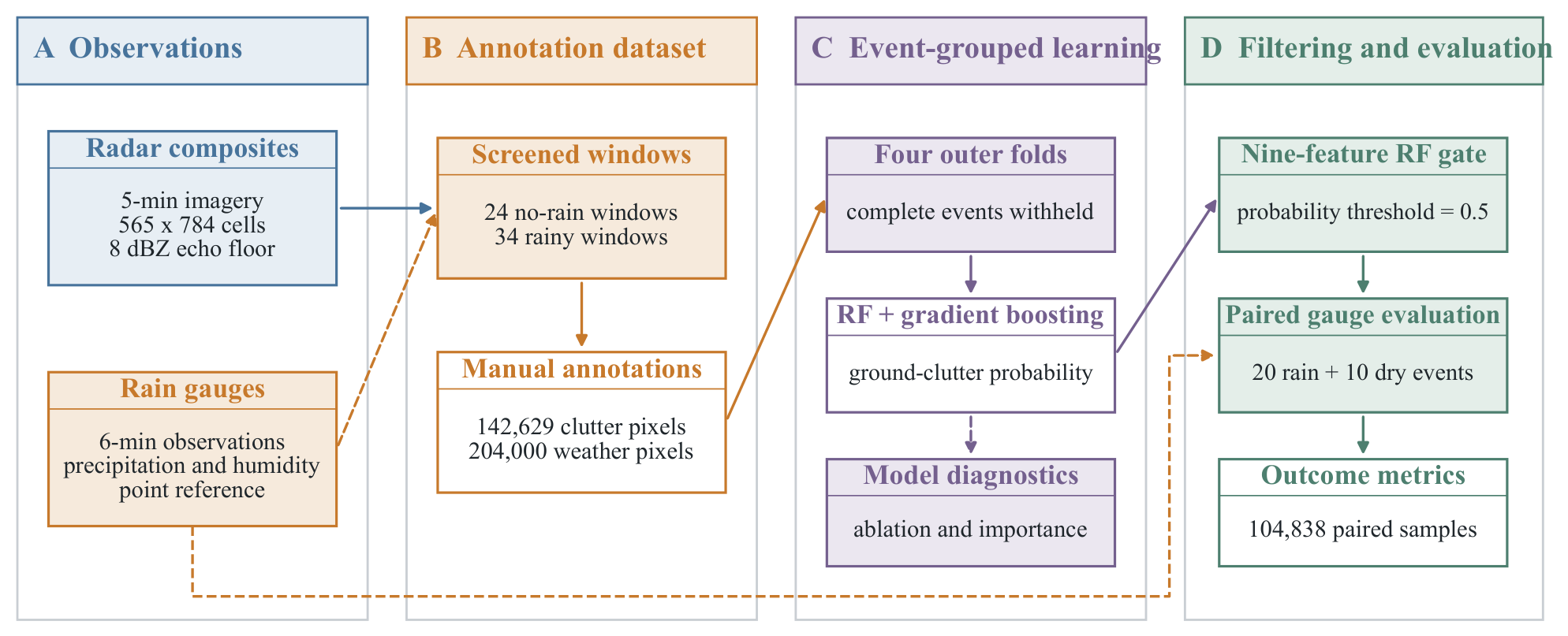
Figure 2.
Feature construction, event-grouped learning, and echo-gating sequence. Six nominal 5-min scans define the 30-min window. Spatial, temporal, and object descriptors are passed to random forest (RF) and gradient-boosted decision tree (GBDT) classifiers; complete target events are excluded during out-of-fold evaluation. The fixed probability decision produces a filtered reflectivity field, followed by an auxiliary paired 30-min quantitative precipitation estimation (QPE) check against gauges.
Figure 2.
Feature construction, event-grouped learning, and echo-gating sequence. Six nominal 5-min scans define the 30-min window. Spatial, temporal, and object descriptors are passed to random forest (RF) and gradient-boosted decision tree (GBDT) classifiers; complete target events are excluded during out-of-fold evaluation. The fixed probability decision produces a filtered reflectivity field, followed by an auxiliary paired 30-min quantitative precipitation estimation (QPE) check against gauges.
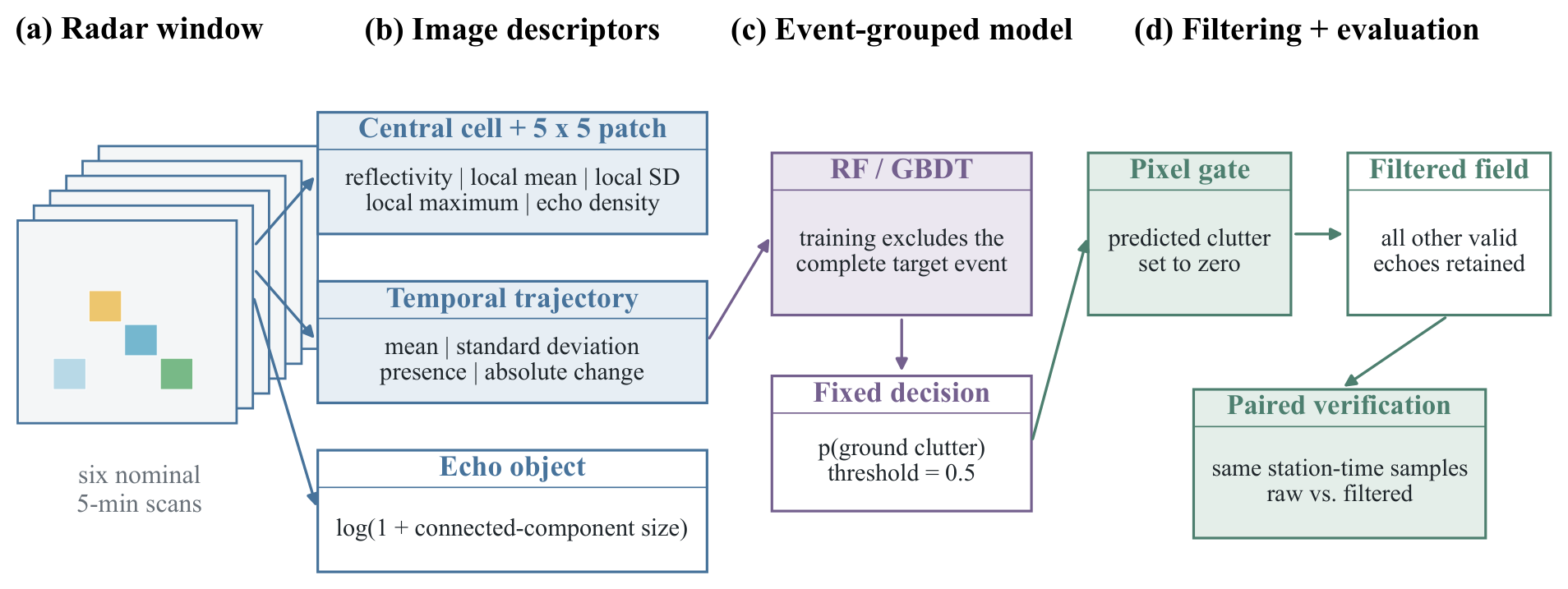
Figure 3.
Study-area location and recurrent clear-air echo structure. (a) Northwestern France radar-composite domain (– N, W– E), with boundaries from Natural Earth 1:10m data. (b,c) Event-weighted recurrence frequency at 5 and 10 dBZ thresholds. Open circles denote the 250 retained gauges, and the orange contour marks recurrence frequency 0.50.
Figure 3.
Study-area location and recurrent clear-air echo structure. (a) Northwestern France radar-composite domain (– N, W– E), with boundaries from Natural Earth 1:10m data. (b,c) Event-weighted recurrence frequency at 5 and 10 dBZ thresholds. Open circles denote the 250 retained gauges, and the orange contour marks recurrence frequency 0.50.
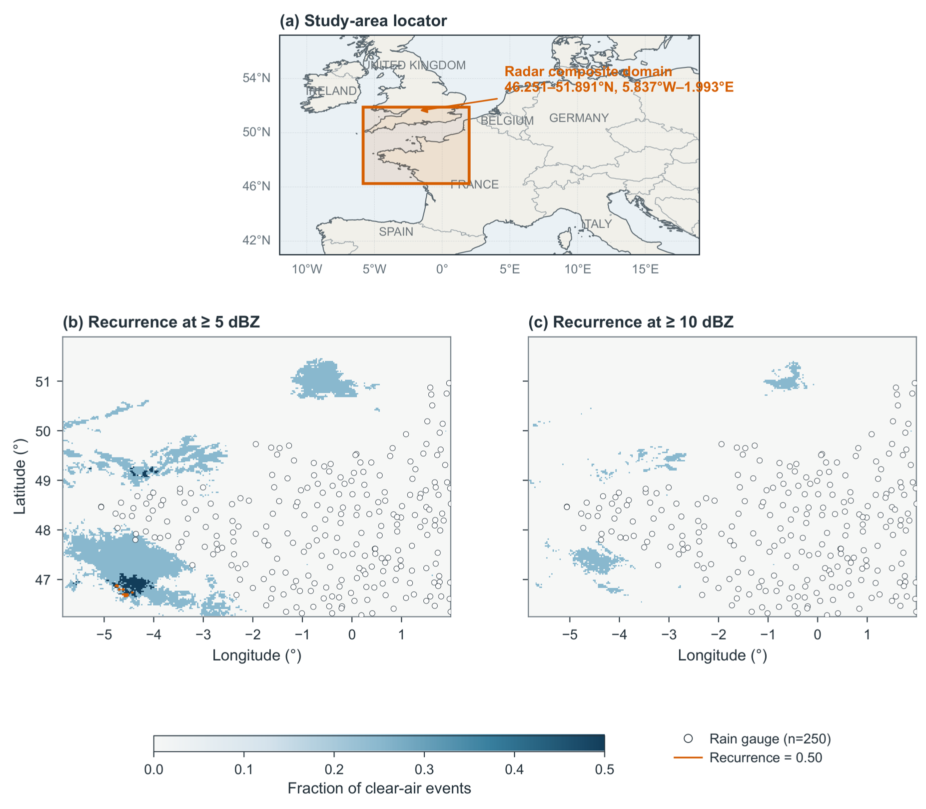
Figure 4.
Event-grouped discrimination curves from concatenated out-of-fold probabilities. (a) Receiver-operating-characteristic curves; (b) precision–recall curves. ROC-AUC values are shown in the shared legend.
Figure 4.
Event-grouped discrimination curves from concatenated out-of-fold probabilities. (a) Receiver-operating-characteristic curves; (b) precision–recall curves. ROC-AUC values are shown in the shared legend.
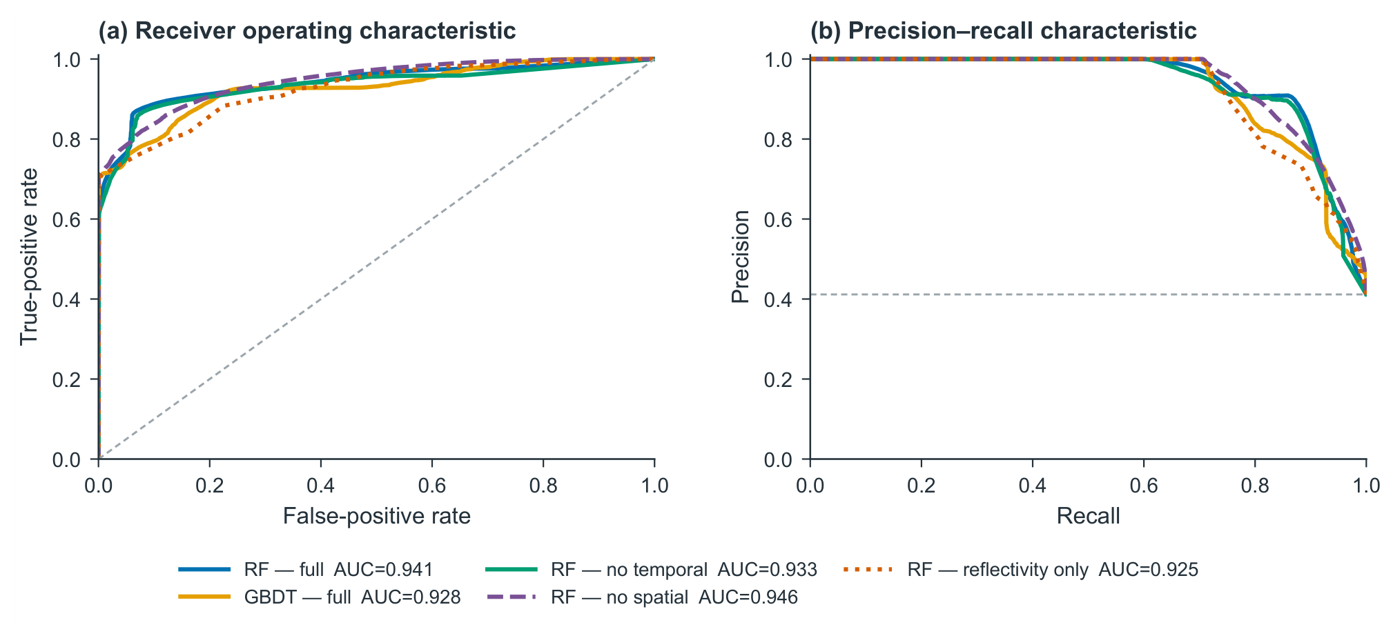
Figure 5.
Full-RF ground-clutter classification diagnostics. (a) Row-normalized confusion matrix from concatenated out-of-fold predictions, with proportions and pixel totals. (b) Event-fold permutation importance, expressed as the decrease in balanced accuracy after one feature was shuffled within a held-out fold. Open circles show individual folds, diamonds show fold means, horizontal intervals span the fold range, and colours identify feature families.
Figure 5.
Full-RF ground-clutter classification diagnostics. (a) Row-normalized confusion matrix from concatenated out-of-fold predictions, with proportions and pixel totals. (b) Event-fold permutation importance, expressed as the decrease in balanced accuracy after one feature was shuffled within a held-out fold. Open circles show individual folds, diamonds show fold means, horizontal intervals span the fold range, and colours identify feature families.
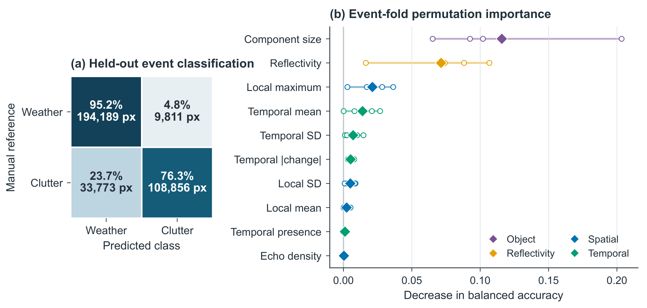
Figure 6.
Out-of-event comparison at 11:00 UTC on 6 May 2016 (outer fold 1). Panels show (a) original reflectivity, (b) local-density-rule filtering, (c) temporal-persistence-rule filtering, (d) RF filtering, (e) GBDT filtering, and (f) the spatiotemporal rule. The retained percentage is the fraction of raw echo pixels at or above 8 dBZ that remains.
Figure 6.
Out-of-event comparison at 11:00 UTC on 6 May 2016 (outer fold 1). Panels show (a) original reflectivity, (b) local-density-rule filtering, (c) temporal-persistence-rule filtering, (d) RF filtering, (e) GBDT filtering, and (f) the spatiotemporal rule. The retained percentage is the fraction of raw echo pixels at or above 8 dBZ that remains.
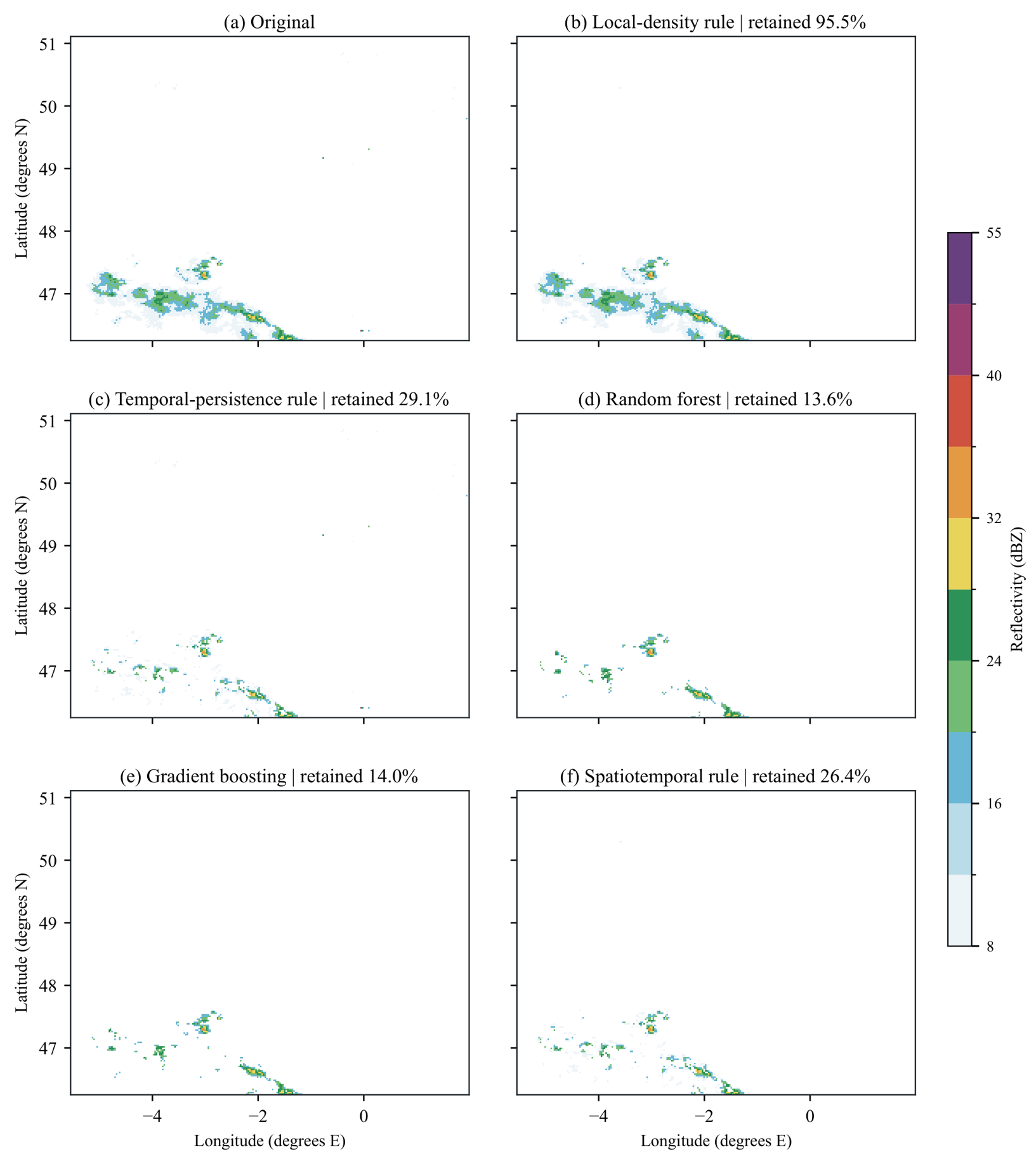
Figure 7.
As in Figure 6, but at 15:00 UTC on 8 May 2016 (outer fold 2). RF retained a larger fraction of this scene than GBDT, indicating between-event sensitivity that is not represented by pooled pixel metrics.
Figure 7.
As in Figure 6, but at 15:00 UTC on 8 May 2016 (outer fold 2). RF retained a larger fraction of this scene than GBDT, indicating between-event sensitivity that is not represented by pooled pixel metrics.
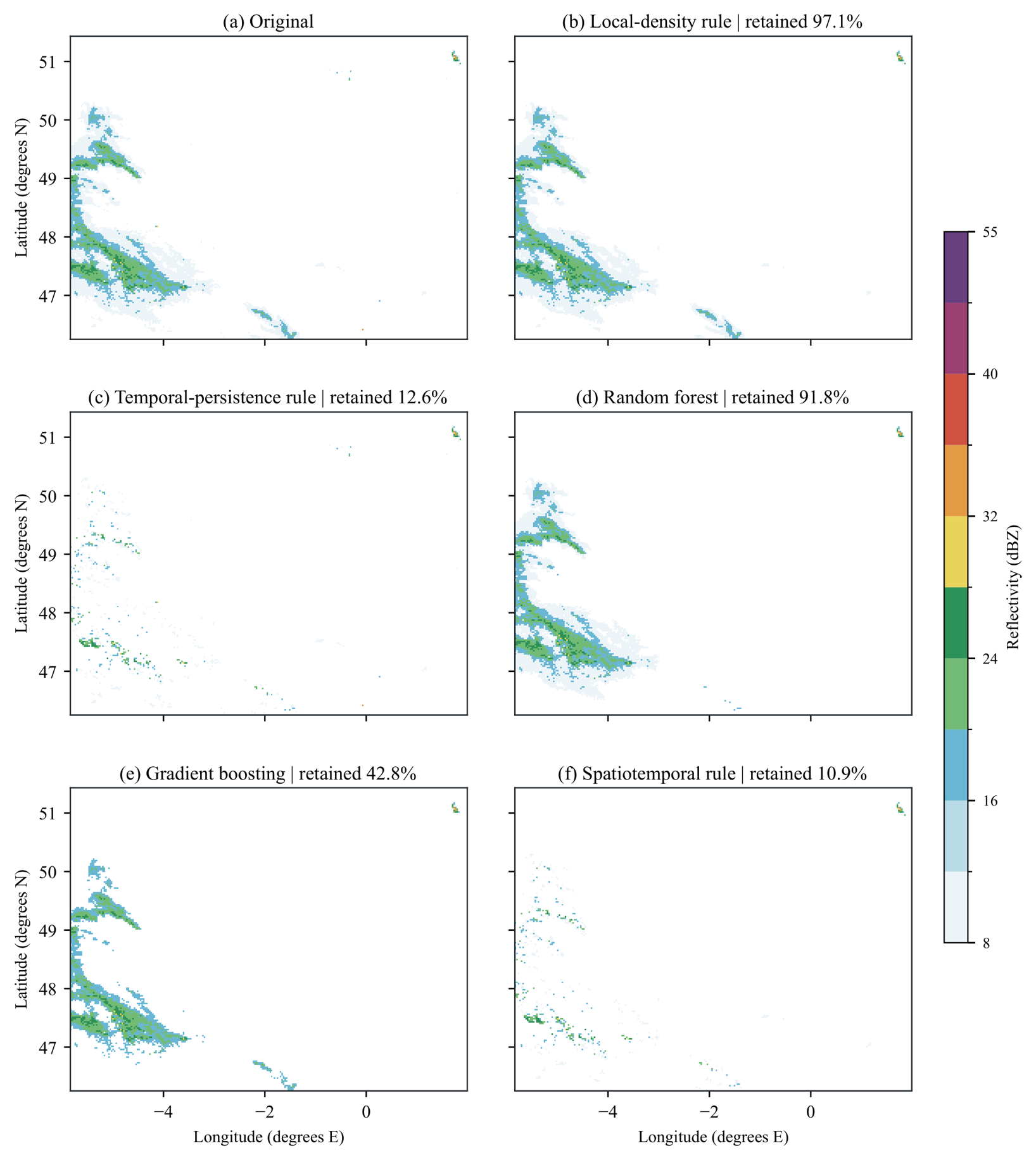
Figure 8.
As in Figure 6, but at 18:30 UTC on 24 May 2016 (outer fold 3). RF retained 3.7% of the raw echo area, the smallest fraction among the learned filters in this event.
Figure 8.
As in Figure 6, but at 18:30 UTC on 24 May 2016 (outer fold 3). RF retained 3.7% of the raw echo area, the smallest fraction among the learned filters in this event.
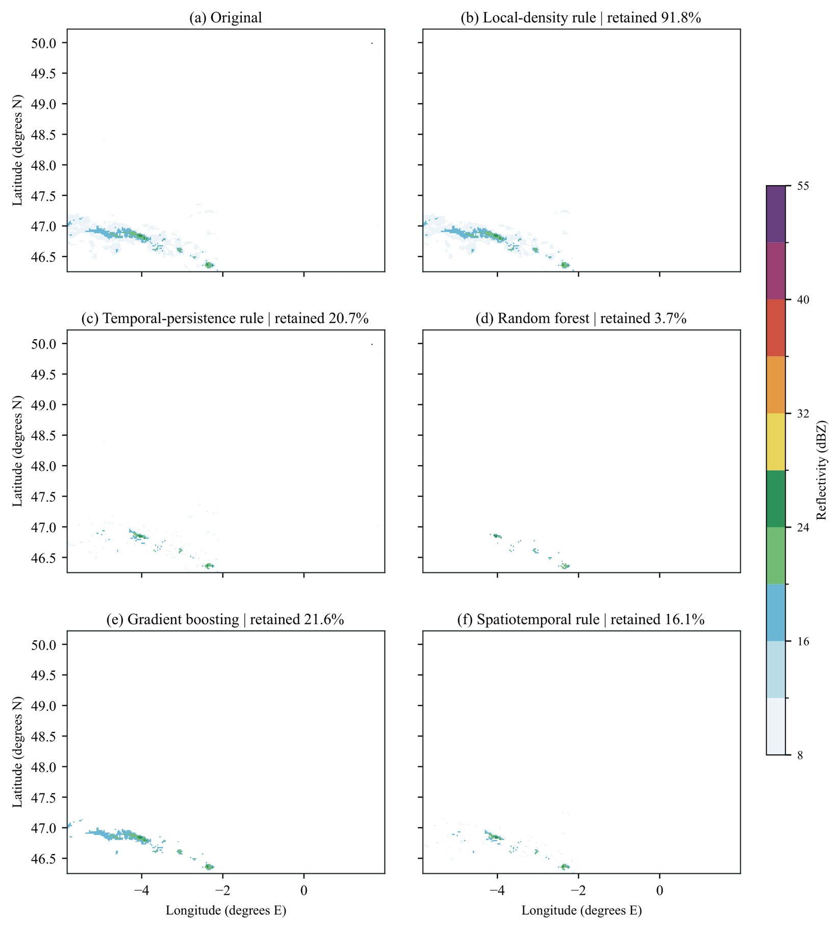
Figure 9.
As in Figure 6, but at 19:30 UTC on 3 November 2016 (outer fold 4). The spatially separated echo clusters provide a distinct morphology from the May cases.
Figure 9.
As in Figure 6, but at 19:30 UTC on 3 November 2016 (outer fold 4). The spatially separated echo clusters provide a distinct morphology from the May cases.
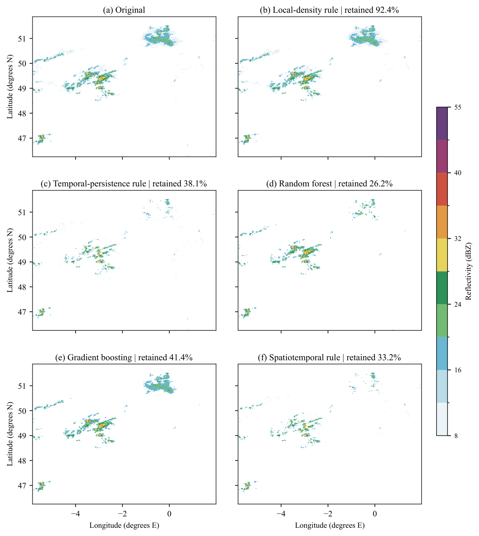

Table 1.
Reflectivity-derived features used by the full classifiers.
| Feature | Definition |
|---|---|
| Reflectivity | Central-scan reflectivity at the target cell (dBZ) |
| Local mean | Mean central-scan reflectivity in a neighborhood |
| Local standard deviation | Standard deviation in the same neighborhood |
| Local maximum | Maximum reflectivity in the neighborhood |
| Local echo density | Fraction of neighborhood cells with reflectivity dBZ |
| Temporal mean | Mean target-cell reflectivity over the 30-min window |
| Temporal standard deviation | Standard deviation over the window |
| Temporal presence | Fraction of scans with target-cell reflectivity dBZ |
| Temporal absolute change | Mean absolute reflectivity difference between consecutive scans |
| Component size | Natural logarithm of one plus the central-scan connected-component size |
Table 2.
Four-fold out-of-event classification against manual pixel annotations. Rule parameters were selected using only the corresponding outer training folds. All values are calculated from concatenated held-out predictions.
Table 2.
Four-fold out-of-event classification against manual pixel annotations. Rule parameters were selected using only the corresponding outer training folds. All values are calculated from concatenated held-out predictions.
| Variant | Suppress. | Preserv. | Precision | CSI | F1 | MCC |
|---|---|---|---|---|---|---|
| Local-density rule | 0.068 | 0.998 | 0.954 | 0.068 | 0.127 | 0.192 |
| Temporal-persistence rule | 0.786 | 0.417 | 0.485 | 0.429 | 0.600 | 0.212 |
| Spatiotemporal rule | 0.826 | 0.415 | 0.497 | 0.450 | 0.620 | 0.255 |
| RF, all features | 0.763 | 0.952 | 0.917 | 0.714 | 0.833 | 0.742 |
| GBDT, all features | 0.773 | 0.934 | 0.891 | 0.706 | 0.828 | 0.726 |
| RF, no temporal | 0.753 | 0.949 | 0.912 | 0.702 | 0.825 | 0.729 |
| RF, no spatial | 0.872 | 0.862 | 0.815 | 0.728 | 0.843 | 0.727 |
| RF, reflectivity only | 0.760 | 0.930 | 0.883 | 0.691 | 0.817 | 0.710 |
Table 3.
Auxiliary paired 30-min raw and targeted-RF QPE at the nine manually confirmed recurrent-clutter stations.
Table 3.
Auxiliary paired 30-min raw and targeted-RF QPE at the nine manually confirmed recurrent-clutter stations.
| Group | Method | N | MAE (mm) | RMSE (mm) | POD | FAR | CSI |
|---|---|---|---|---|---|---|---|
| Confirmed sites | Raw | 4014 | 0.055 | 0.283 | 0.635 | 0.277 | 0.511 |
| Targeted RF | 4014 | 0.052 | 0.284 | 0.738 | 0.181 | 0.635 |
Disclaimer/Publisher’s Note: The statements, opinions and data contained in all publications are solely those of the individual author(s) and contributor(s) and not of MDPI and/or the editor(s). MDPI and/or the editor(s) disclaim responsibility for any injury to people or property resulting from any ideas, methods, instructions or products referred to in the content. |
© 2026 by the authors. Licensee MDPI, Basel, Switzerland. This article is an open access article distributed under the terms and conditions of the Creative Commons Attribution (CC BY) license (http://creativecommons.org/licenses/by/4.0/).
Copyright: This open access article is published under a Creative Commons CC BY 4.0 license, which permit the free download, distribution, and reuse, provided that the author and preprint are cited in any reuse.