
Submitted:
28 August 2026
Posted:
28 August 2026
You are already at the latest version
Abstract
Validation-based machine-learning model selection in temporally dependent, weak-signal data can produce a clear numerical winner without sufficient evidence that the choice will remain reliable out of sample. This study develops PC-Audit (Prequential-Calibration Audit), a decision-reliability framework for auditing the evidence behind validation-selected model choices. The framework combines target-date partitioning, prequential non-negative calibration, Model Confidence Sets (MCS), transfer diagnostics, dependence-aware inference, cost and execution checks, temporal stress testing, and fallback simulation. It is evaluated on nine Chinese index ETFs in 45 walk-forward cases from 2020 to 2024 under a controlled CPU-only setting. For signed returns, mean validation-to-test rank correlation is 0.090, PC-Select identifies the lowest-test-MAE candidate in 15 of 45 cases, the label-permutation value is p=0.0521, and the prequential MCS retains 4.80 of five candidates. No Holm-adjusted MAE reduction is found relative to naive references or individual-model baselines. Volatility-like targets show stronger main-period ranking transfer, but rolling/EWMA references remain competitive and 2025 stress weakens the evidence. Audit-triggered fallback does not improve mean MAE but modestly reduces worst-year MAE. PC-Audit therefore provides an auditable and reproducible reliability layer for validation-based time-series model selection rather than a forecasting-accuracy enhancement method.
Keywords:
machine-learning model selection
; decision reliability
; model auditing
; time-series evaluation
; prequential calibration
; Model Confidence Set
; machine-learning deployment
; financial time series
1. Introduction
Validation-based machine-learning model selection is a routine step in deployment: several candidate models are trained on historical data, one is chosen using a finite validation interval, and the selected candidate is then carried forward to a later operating period. In temporally dependent and weak-signal settings, however, the existence of a numerical validation winner does not by itself establish that the choice is reliable. Candidate errors may be close, observations are serially dependent, regimes can change, and a short validation segment may appear decisive even when it contains little information about the next period.
Financial time series provide a particularly demanding setting for this problem. Daily index-ETF returns have low signal-to-noise ratios, broad-market information is incorporated quickly, and small apparent performance differences can be sensitive to calibration, execution assumptions, and market regime. These features make financial prediction a useful stress test for a broader evaluation question: whether the evidence behind a validation-selected machine-learning action is strong enough to support a deployment interpretation.
Most empirical studies naturally emphasize predictive accuracy, model architecture, hyperparameter choice, or trading outcomes. Considerably less attention is given to the reliability of the selection act itself: whether the model chosen on validation data is statistically distinguishable from alternatives, whether the ordering transfers out of sample, and whether the resulting interpretation survives dependence, multiplicity, cost, execution, and temporal stress. Without such checks, a routine validation winner can be overinterpreted as stable deployment evidence.
This paper addresses that narrower methodological gap. The aim is not to search for a universally strongest predictor or to claim an investable ETF timing rule, but to construct an auditable framework that determines how strongly a validation-selected candidate can be interpreted before deployment. The central idea is to treat model selection as a decision object: the selected model name must be reported together with calibration timing, confidence-set uncertainty, validation-to-test transfer, regret, cost and execution stress, temporal-holdout behavior, and an audit-state record that can inform the next review cycle.
Time-aware partitioning is necessary but not sufficient. A next-day target must be assigned to a split according to the date of the predicted return, not only the date of the feature row. Prediction-scale mismatch also complicates model comparison: a recurrent or tree model may have useful ordering information but an unstable amplitude. Calibration can correct amplitude, yet fitting and scoring a calibration coefficient on the same validation outcomes creates optimistic losses. Finally, selecting the numerically lowest validation error hides uncertainty when several candidates are statistically indistinguishable.
To address these issues, PC-Audit (Prequential-Calibration Audit) evaluates validation-driven model selection as a pre-deployment decision. The framework combines target-date partitioning, chronological prequential calibration, a moving-block-bootstrap Model Confidence Set (MCS), validation-to-test diagnostics, dependence-aware inference, transaction-cost and execution checks, computational-cost reporting, and a fixed 2025 temporal stress evaluation. PC-Select is the operational rule that identifies one candidate using the audit-defined validation loss; it is not an additional forecasting model. The remaining components quantify the uncertainty and practical limits surrounding that action. Thus, the framework is useful even when the evidence is insufficient to support a strong deployment interpretation.
The framework imposes three requirements. First, the selected action must arise from a leakage-controlled validation rule. Second, its uncertainty must be reported through confidence-set and transfer diagnostics. Third, any economic or cost-related interpretation must remain conditional on multiplicity, dependence, execution, sensitivity, and temporal-stress evidence. These requirements turn model selection into a falsifiable decision protocol: the evidence may support, qualify, or reject the proposed deployment action. PC-Audit contributes a prespecified decision-reliability architecture for validation-based model selection. It combines leakage-controlled selection, prequential calibration, uncertainty-set assessment, transfer diagnostics, and forward-only governance within a common information boundary. Its novelty lies in how these components are ordered and constrained around the validation-selected action as the explicit audit object. The constituent statistical procedures are individually established; no claim is made that any single calibration, bootstrap, or confidence-set procedure is new.
The study answers three audit questions:
- 1.
- Does a leakage-controlled validation rule provide sufficient signed-return deployment evidence when confidence-set uncertainty, selection margin, rank transfer, hit rate, regret, and competing baselines are jointly audited?
- 2.
- Are volatility-like risk-surveillance targets more auditable than signed returns under the same protocol, and do they remain bounded under strong rolling/EWMA references and 2025 stress?
- 3.
- Can completed audit outputs be carried forward as monitoring variables and fallback actions for the next deployment review without turning the benchmark into an online learner?
The contribution is threefold. First, the paper treats the validation-selected candidate as an explicit audit object and integrates calibration-timing control, MCS-based uncertainty assessment, selection-margin analysis, validation-to-test transfer diagnostics, dependence-aware inference, and practical stress checks into one reproducible decision-reliability protocol. Second, it shows that the strength of selection evidence differs materially by target type: volatility-like risk-surveillance targets exhibit more stable validation-to-test evidence than signed daily returns under the same leakage-controlled design, while strong rolling and EWMA references remain competitive. Third, it introduces a forward-only audit state and fallback simulation that use completed-year evidence to inform the next scheduled review without tuning the reported test results. Together, these contributions provide an operational evidence framework for assessing when a validation-selected candidate warrants a stronger or weaker deployment interpretation. Raw snapshots, features, prediction caches, scripts, intermediate tables, and file hashes are supplied for verification.
Table 1 summarizes how the design addresses common evaluation risks in weak-signal time-series machine learning. The table is included to make the claim boundary explicit: each protocol component either removes a possible source of optimism or defines when a positive interpretation is not warranted.
2. Related Work
Machine learning has been applied extensively to financial time-series prediction, from regularized linear models and tree ensembles to recurrent and deep architectures [1,2,3,4]. Recent benchmark studies also examine larger time-series and foundation-model families [5,6]. These studies establish the candidate-model background for this work, but architectural breadth does not resolve the evaluation problem created by validation-based selection. PC-Audit therefore focuses on the reliability of the decision produced by model selection rather than on proposing another forecasting architecture.
Evaluation protocol is a central issue for temporally dependent data. Random cross-validation can mix temporal information and misrepresent deployment conditions, whereas rolling-origin or walk-forward evaluation preserves the forward-looking structure of the task [7,8,9]. Leakage-controlled financial benchmarks further emphasize train-only preprocessing, causal feature construction, strong naive references, and conservative conclusions when signed-return prediction remains close to baseline performance [10]. PC-Audit extends this evaluation logic by asking whether the deployment interpretation created by validation-based selection is supported by uncertainty, transfer, and stress evidence. Its audit object is the selection decision itself, not only the forecast error of each candidate.
A second stream studies model-selection risk. Even when several models are reasonable on average, a short validation segment may have low probability of identifying the best next-period forecaster [11]. This problem is related to backtest overfitting, research-protocol discipline, and multiple-testing risk in financial research, where repeated searching can create attractive but fragile results [12,13,14,15]. The present study therefore reports top-one hit rate, validation-to-test rank correlation, selection regret, and permutation evidence rather than treating the lowest validation MAE as self-justifying.
Uncertainty-aware model comparison provides a complementary foundation. The Model Confidence Set retains models that cannot be rejected as inferior under a specified loss and bootstrap scheme [16]. Its financial forecasting applications show why confidence-set reporting can be more informative than simply naming a best model when the data cannot sharply separate alternatives [17]. PC-Audit uses this property as an audit component: MCS membership constrains the strength of a deployment interpretation, but it is not treated as a forecasting model and does not imply economic profitability.
Resource-aware forecasting and multi-objective model selection have also been studied for time-series systems [18]. PC-Audit is related but distinct. It does not optimize a combined accuracy-cost score or search for a new model family. Instead, it evaluates a fixed candidate pool in a controlled CPU-only setting and asks whether the validation-selected action remains defensible after calibration timing, statistical uncertainty, transfer diagnostics, costs, execution delay, sensitivity variants, and temporal stress are audited.
Related work on Machine Learning Operations (MLOps) and ML lifecycle management broadens the evaluation perspective from model development to reproducible deployment, monitoring, versioning, and feedback across the operational lifecycle [19,20]. PC-Audit is complementary to this literature but targets a narrower upstream decision: before a validation-selected candidate is interpreted as deployable, how strong is the evidence supporting that selection? Its audit-state mechanism records completed evidence for the next scheduled review while preserving the information boundary of the current test period. The framework does not replace end-to-end MLOps infrastructure, continuous integration, or production monitoring; it supplies a prespecified model-selection audit layer that can be embedded within such lifecycle processes.
The remaining gap is therefore not the absence of forecasting architectures or individual statistical tools. Existing work provides time-aware evaluation methods, model-selection diagnostics, MCS uncertainty procedures, and warnings about overfitting, but these elements are seldom organized around the validation-selected action itself as the object of audit. PC-Audit addresses this gap by integrating them into a reproducible evidence architecture that can support, qualify, or reject a deployment interpretation and can carry completed audit outputs forward to the next review cycle without retroactively tuning reported test results.
3. Materials and Methods
Figure 1 summarizes the order in which information enters the audit. It separates model fitting and validation selection from the evidence used to judge that selection, and it shows that completed test outcomes are carried forward only as governance inputs for the next review cycle. Algorithm 1 states the case-level protocol used for each ETF-window split. The 2025 split repeats the same fixed procedure once as a temporal stress test.
| Algorithm 1 PC-Audit for one ETF-window case |
|
3.1. Audit Design, Data Provenance, and Target-Date Partitioning
PC-Audit is organized as a fixed pre-deployment audit of validation-based model selection. The dataset is treated as an immutable benchmark input; the ETF universe, coverage, and row counts are reported with the experimental results in Table 2 so that the Methods section can focus on the audit logic. Although the public data vendor facilitates reproduction, it is not the exchange’s official historical database [21]. To prevent later vendor revisions from changing the experiment, the package stores the exact snapshots and file hashes. This supports computational replication while leaving one-vendor dependence and vendor-revision risk as limitations. We do not claim that the dataset is survivorship-free.
Throughout the paper, t indexes the date on which a target is realized. Let denote the ETF closing price on trading date t. The close-to-close return realized on that date is
At the preceding forecast origin , the future price and hence are not yet observed; they become available only when the target is labeled for evaluation. Let denote the feature vector constructed solely from information observed no later than date . It contains lagged returns, rolling moments, momentum, price ranges, volume changes, moving-average ratios, and the technical indicators listed in the configuration file. Missing values introduced by rolling windows are removed deterministically.
Let denote the target realized on date t. For the primary signed-return audit, . Candidate model m maps the lagged feature vector to a one-step-ahead prediction,
where is the prediction function fitted for candidate m and is its raw prediction of . Thus, no quantity dated t is used as an input when predicting the target at date t.
The signed-return target remains the primary audit case because it corresponds to the common deployment question of whether a validation-selected model supports a directional interpretation. As a risk-surveillance extension, the same fixed pipeline is also run on three volatility-like targets:
where is absolute return, is squared return, is a high–low range proxy, and and are respectively the high and low prices on target date t. For each extension, is replaced by the corresponding target. These targets are evaluated with prediction-scale losses, rank transfer, MCS size, and selection regret. They are not used for directional accuracy, transaction-cost signal returns, or trading-performance claims. In the robustness scripts, target-derived columns are explicitly excluded from before model fitting, so the alternative targets remain prediction targets rather than predictors.
Each observation stores both its feature date and target date t. Split membership is assigned by the target date, preventing a final training feature row from carrying a validation-period outcome and a final validation row from carrying a test-period outcome. Formally,
where , , and are the training, validation, and test sets, while and are the target-date cutoffs ending the training and validation windows. This target-date convention is used in all subsequent equations.
The outer design uses five years for training, one year for validation, and one year for testing. Test years 2020–2024 produce ETF-window cases. A sixth fixed split trains on 2019–2023, validates on 2024, and tests on 2025. The 2025 split is a temporal stress test, not an independent market or data-provider sample.
3.2. Candidate Models and Prequential Calibration
The candidate pool contains ElasticNet, Ridge, LightGBM, Random Forest, and a small GRU [22,23,24,25,26]. Hyperparameters are fixed in model_configs.json and are not retuned on test years. The GRU receives causal 10-trading-day sequences; validation and test sequences use only preceding context. All models run on CPU.
The pool represents common low-cost prediction models with different inductive biases: regularized linear models, tree ensembles, boosting, and a compact recurrent network. It is not an exhaustive architecture benchmark. The object of study is the audited selection protocol, not a new model architecture or a search for the globally strongest predictor. To avoid attributing weak separation only to the use of individual models, the extended analysis also includes simple historical-prediction and prediction-aggregation references. Larger alternatives such as transformer-style sequence models, additional boosting variants, or broad hyperparameter searches are left outside the default pool because they would change the study from a CPU-only deployment audit into a model-zoo search and would increase selection and multiple-testing risk.
Let denote the fixed candidate-model pool, where . For target date t, is the raw prediction of candidate . To address prediction-scale mismatch, calibration uses a non-negative scalar estimated from an explicit information set. For a calibration index set , define
The set is the slope-estimation information set. Non-negativity permits shrinkage to zero, but no arbitrary upper cap; a zero slope means that the available sample supports the zero forecast among non-negative scalar multiples. The numerical tolerance matches the supplied implementation.
Using the same validation outcomes both to estimate and score calibrated validation predictions would be optimistic. PC-Audit therefore follows a prequential evaluation logic in which predictions are scored only after the information used for calibration is available [27]. It divides the validation year into four contiguous blocks . Block 1 is a warm-up. For each scored block , the available calibration history is
and the block-specific prequential slope is
Thus, is estimated only from validation labels that occur before block b, and the corresponding validation prediction is . The prequential absolute loss for model m at scored validation date t is
where is the validation block containing date t. PC-Select is the audit-defined deployment recommendation: it names the candidate with the lowest mean but does not by itself imply that the selected candidate is statistically separated from the alternatives. Let
where is the mean prequential validation MAE for model m over the scored validation blocks. The first, selection-stage decision is
Exact ties are resolved by the fixed candidate order recorded in the supplied implementation. After the validation year has fully elapsed, the selected model receives one final deployment-time calibration on the complete validation set :
The first stage selects without same-label calibration bias; the second estimates the selected candidate’s deployment scalar after validation is complete, before the test year begins. It neither changes the selected model nor reuses test outcomes; the remaining audit diagnostics govern how strongly the choice may be interpreted.
3.3. Confidence Sets, Transfer Diagnostics, and Deployment Checks
For each case, a moving-block-bootstrap MCS is computed from the candidate loss matrix
where each row corresponds to a candidate model and each column corresponds to a scored validation date. The default prequential-loss MCS uncertainty audit uses , the prequential absolute loss defined above. The MCS is estimated using the maximum-t statistic, , 5000 bootstrap repetitions, and block length approximately equal to the square root of the evaluated validation length [16,17,28]. The 10% level is used as a screening-oriented confidence-set threshold rather than as a declaration of model separation; 5% and 20% alternatives and block-length multipliers of 0.5, 1, and 2 are included in the sensitivity audit. The lowest prequential-MAE model remains the deployment rule; MCS membership quantifies uncertainty. Pairwise MCS comparisons are based on loss differences
where means that model i has lower loss than model j on date t. The audit therefore asks whether observed differences among candidates are statistically distinguishable under the specified dependent-data bootstrap.
Two controls isolate calibration timing. The raw-loss MCS uncertainty audit uses uncalibrated errors on the same post-warm-up validation observations. The same-label calibrated MCS fits one coefficient on the complete validation year and evaluates it on those same labels. The MCS equal-weight comparator averages the individually final-calibrated test predictions of the prequential-loss MCS members:
No test outcome enters either member calibration or the average. The raw-loss selector, same-label selector, individually calibrated candidates, zero-return predictor, historical-mean predictor, and full five-model ensemble average are comparators. The last two are low-cost reference checks derived from available historical targets and saved candidate predictions; they are not tuned on the test period.
For any test index set , prediction-scale errors are computed from the final-calibrated prediction . The root-mean-square error and mean absolute error for model m are
and
where is the test-period date set for one ETF-window case. Direction is evaluated using directional accuracy (DA), balanced accuracy (BA), and Matthews correlation coefficient (MCC). Define the realized sign label and predicted sign label as
where equals one when the condition is true and zero otherwise. Then
BA and MCC are computed from true positives (), true negatives (), false positives (), and false negatives ():
and
These directional metrics prevent an always-zero or always-down forecast from appearing skillful solely because of class imbalance. The supplied implementation uses the deterministic conventions of scikit-learn: if MCC has a zero denominator, it is returned as zero; if only one observed class is present, BA is the recall of that observed class. Both conventions are recorded rather than silently replacing an undefined value.
For each ETF-window case c, validation candidate ranks are compared with test-MAE ranks. Let be the prequential validation loss of model m, and let be its test MAE. Let be the rank of among , and let be the rank of among , with rank 1 assigned to the smallest loss. The case-level validation-to-test rank correlation is then the ordinary Pearson correlation applied to these two rank vectors:
where and . This is the Spearman rank correlation written explicitly rather than treated as a named black-box function. Annual summaries average over the ETF-window cases completed in year k.
The top-one hit indicator for case c is
so an exact tie for the lowest test MAE counts as a hit. The reported top-one hit rate is the average of over the evaluated cases. A uniform five-model reference is 20%; a label-permutation audit additionally preserves the observed frequencies of selected and lowest-test-loss model labels, with a within-ETF permutation as a dependence-oriented control. Selection regret is the selected model’s test loss minus the best attainable test loss within the candidate pool:
where is an ex post candidate-pool minimum, not an additional candidate model. Regret is non-negative and equals zero only when PC-Select chooses a lowest-test-MAE candidate. MCS coverage records whether a lowest-test-MAE candidate was retained by the validation MCS.
Paired comparisons use two-sided Wilcoxon signed-rank tests. Holm correction is applied over the prespecified predictive comparison family. Since the 45 cases share ETFs, years, and overlapping training intervals, mean-difference intervals are also obtained by resampling ETFs as clusters and test years as blocks. The interpretation rules are applied conservatively and are allowed to return a negative or inconclusive audit outcome.
Signal diagnostics use the sign of the prediction to form an unlagged long-short proxy and one-day-lagged long-cash and long-short controls. Turnover costs of 0, 5, 10, and 20 bps are deducted. These are stress diagnostics, not implementable trading claims. Because the study is motivated by resource-constrained deployment, predictive and signal metrics are reported together with computational cost rather than collapsed into a single optimized score. No utility-cost score is tuned on the test period, and no favorable cost summary is allowed to override weak predictive, dependence-aware, or temporal-stress evidence.
Sensitivity analysis varies validation blocks (3–6), MCS significance (0.05, 0.10, 0.20), loss (absolute or squared), block-length multiplier (0.5, 1, 2), and calibration rule (non-negative, unconstrained, or the legacy clipped rule). Saved prediction caches are used without retraining so that sensitivity differences reflect the audit protocol rather than changes in fitted candidate models. The default four-block absolute-error non-negative protocol was fixed before sensitivity analysis and is retained even when another variant gives a more attractive economic proxy.
To make the audit falsifiable, each positive interpretation requires evidence beyond a favorable average. A lower-error claim requires a multiplicity-adjusted comparison and dependence-aware intervals pointing in the same direction. Reliable selection requires both nontrivial top-one evidence and validation-to-test rank-transfer intervals excluding zero. Economic deployability requires consistent signs under transaction costs, one-day execution delay, protocol sensitivity variants, and the 2025 stress split. When these conditions are not met, the manuscript reports the result as weak, mixed, or unsupported rather than treating a favorable single metric as a discovery.
3.4. Deployment-Cycle Audit-State Construction and Reproducibility
PC-Audit is not implemented as an online learner in this benchmark. No model is retrained, no hyperparameter is retuned, and no reported test-year result is revised using realized test outcomes. To distinguish the annual review-cycle index from the target variable , let k index a completed test year. After year k has ended, its realized audit outputs are logged as monitoring variables for the next scheduled review in year . This construction represents a feedback mechanism at the audit-governance level rather than at the model-fitting level.
Signed-return and volatility-proxy audits are separate. Let identify the target and define the completed-case state
where is MCS size, records selection–MCS membership, is rank transfer, and is regret. The stress components use opposite favorable directions: larger is favorable for the unlagged 20-bps signed-return proxy , whereas smaller is favorable for , PC-Select MAE minus EWMA(0.97) MAE. For completed year k, let denote its nine ETF-window cases. Its annual components are
The annual audit-state summary is
The selected-model identity is retained in each case record but is categorical and therefore not numerically averaged into . The next-cycle deployment interpretation is then a target-specific deterministic function of the completed-year audit state:
The reported simulation uses four warning indicators for each target:
The four warnings flag weak separation, nonpositive transfer, regret above a fixed tolerance, and target-specific adverse stress. is a descriptive selection–MCS coherence measure, intentionally excluded from the traffic-light count because no threshold was prespecified. The warning count is
The traffic-light rule is then
Green maintains a cautious selected-model interpretation, Yellow calls for review, and Red recommends fallback or re-audit. These conservative thresholds are fixed, not fitted, retrospective audit rules: means that nearly all candidates remain indistinguishable; means no positive ordering evidence; and marks loss relative to the candidate-pool minimum. For signed returns, flags a nonpositive high-cost proxy; for volatility, means PC-Select is worse than EWMA(0.97). Requiring three warnings avoids a full re-audit after one noisy diagnostic. All variables are carried forward only after the corresponding test year ends.
The fallback simulation converts this interpretation state into a fixed next-year action within the reported retrospective exercise. Let and denote the actions applied in year for the signed-return and volatility-proxy audits, respectively. For signed returns,
For the volatility-proxy audit, where strong naive volatility references are available,
where Naive-Select chooses among Roll-10, Roll-21, Roll-63, EWMA(0.94), and EWMA(0.97) using only the preceding validation year. These fallback rules are not optimized on the test years; they test whether audit states can guide conservative next-cycle governance without claiming to improve current-year accuracy.
To test whether the audit could instead support retaining or replacing the current-year PC-Select action, a separate falsification analysis uses only information available at deployment: prequential validation MCS size, the relative validation margin, and the frequency with which the final selected model wins the three scored chronological validation blocks. The validation-only score components are defined in Supplementary Equation S1; the information boundary and risk–coverage evidence are reported in Supplementary Table S5, Supplementary Figure S2, and Supplementary Table S6. Test regret, validation-to-test transfer, candidate-pool minimum coverage, and current test outcomes are excluded from score construction and are used only for evaluation. The analysis compares the three individual signals with the equal-weight score over their full risk–coverage paths. This is a falsification of hypothetical prospective filtering, not an additional model-selection stage.
The experiment used Linux x86_64, Python 3.13.5, NumPy 2.3.5, pandas 2.2.3, scikit-learn 1.8.0, LightGBM 4.6.0, and CPU-only PyTorch 2.10.0+cpu. The container exposed 56 logical CPU interfaces and 4.0 GB RAM. Exact raw files, feature tables, prediction caches, scripts, configurations, results, audit-state tables, and hashes are included. The supplied checks verify the current headline values against the CSV result files, validate raw-data inventories, test the deterministic MCS implementation, and recompute file hashes.
4. Results
The results are organized to answer the three audit questions rather than to select the most attractive metric. Table 2 fixes the case-study boundary; Table 3, Table 4 and Table 5 evaluate whether signed-return validation selection deserves a strong deployment interpretation; Table 6 and Table 7 examine how validation reliability changes across prediction targets; and Table 9 evaluates the feedback and fallback governance mechanism. Supplementary Tables S1, S2, S3, S4, S5, and S6; Supplementary Figures S1 and S2; and Supplementary Equation S1 supply the detailed tables, window-level records, robustness outputs, and validation-only score definition.
4.1. Data Universe and Predictive Baselines
Table 2 reports the fixed ETF universe used in the audit. The benchmark uses Yahoo Finance daily OHLCV snapshots for nine mainland Chinese index ETFs from 2 January 2014 through 31 December 2025. The objective is not to claim universal applicability across all financial markets, but to provide a controlled case study for deployment-oriented audit methodology. Each raw file contains 2916 unique trading dates. The universe was defined before the PC-Audit analysis using three operational requirements: continuous coverage from the beginning of 2014, no duplicate dates, and representation of broad-market, size, style, growth, and sector exposures. It is a controlled audit benchmark rather than an exhaustive or market-wide sample of Chinese ETFs.
The equal row counts in Table 2 matter for interpretation: differences among models are not driven by unequal sample coverage or ticker-specific missing-history rules. At the same time, the table also defines the external-validity boundary. The benchmark is deliberately narrow enough to support a reproducible audit, but it is not a claim about all Chinese ETFs or all market regimes.
Table 3 reports 2020–2024 averages at zero transaction cost. In all 45 cases, the model named by PC-Select is also retained by the prequential-loss MCS, so the deployable recommendation is not rejected by the confidence-set audit even though the set is usually large. PC-Select records RMSE 0.015821, MAE 0.010593, balanced accuracy 0.49998, and MCC . The directional metrics are effectively at chance.
The naive references are strong on prediction-scale error. The historical-mean reference has the lowest average MAE (0.010546), and the zero-return predictor has slightly lower RMSE (0.015798) and MAE (0.010563) than PC-Select. The paired PC-Select versus zero-return MAE comparison has unadjusted and Holm-adjusted ; ETF-cluster and year-block mean-difference intervals favor the zero reference. Therefore, PC-Select does not establish lower prediction error than naive benchmarks under the present sample. The historical-mean reference also produces a nearly constant sign exposure, so its return proxy is interpreted only as a stress diagnostic rather than as timing skill.
No PC-Select comparison is significant after Holm adjustment. Relative to the same-label calibrated selector, the unadjusted MAE test favors PC-Select (), and both dependence-aware intervals have the same orientation, but the Holm-adjusted value is 0.431. The auxiliary ensemble-average row is deliberately included because it is a common robustness device; here it performs worse than the calibrated single-model references on RMSE and MAE, so the mixed conclusion cannot be dismissed as merely a failure to average candidates. This is suggestive evidence that protocol choices alter selection, not evidence of a universal lower-error advantage. Table 3 therefore functions as a guardrail for the rest of the Results section: subsequent transfer and feedback analyses are interpreted as audit diagnostics, not as proof that PC-Select beats naive prediction.
4.2. Validation Transfer and Statistical Separation
Figure 2 and Table 4 quantify validation-to-test transfer. Under prequential calibration, mean rank correlation is 0.090 and both dependence-aware 95% intervals include zero. PC-Select nevertheless chooses the lowest-test-MAE candidate in 15 of 45 cases (33.3%). The exact binomial diagnostic against a uniform 20% rate gives , but the more conservative global label-permutation audit gives ; the within-ETF permutation gives . We therefore treat the hit rate as limited, borderline transfer evidence rather than a confirmatory discovery. It does not extend to a stable ranking of all candidates and falls to 22.2% in 2025.
The same-label control has a 35.6% hit rate in 2020–2024 but negative mean rank correlation and larger regret. Its apparent top-one success therefore does not imply better global ranking. Across protocols, no method consistently dominates both the main period and 2025.
The weak transfer result is also visible before testing through small validation margins. The audit records the validation margin between the first- and second-ranked candidates under the default prequential loss. Let and denote the smallest and second-smallest values in the set for one ETF-window case. The selection-margin statistic is
In 2020–2024, the median is , the interquartile range is 0 to , and 93.3% of cases have . These small margins explain why naming a single validation winner is operationally possible but statistically fragile. Figure 3 shows the same issue visually: a deployment recommendation can exist even when the scientific claim remains weak, because the selector is forced to name the smallest validation loss but the distance between the first and second candidates is often too small to justify strong language about superiority.
Calibration timing changes the apparent statistical admissibility of candidates. The default prequential MCS contains 4.80 of five candidates on average and retains all five in 38 of 45 cases (84.4%). The raw-loss MCS contains 3.67 models on average and never retains all five. Same-label calibration retains 4.98 and includes all five in 44 cases. Raw and prequential memberships differ in 43 of 45 cases (95.6%); same-label and prequential memberships differ in 17.8%.
Table 5 shows that the more selective raw-loss protocol is not necessarily the more reliable protocol. It removes more candidates, but it also has lower coverage of a candidate that attains the minimum test MAE and almost always changes the confidence set relative to the prequential design. The omitted plot gives the same trade-off visually; the table is kept in the main text because it carries the numerical audit evidence. This is why PC-Audit reports confidence-set composition as uncertainty evidence rather than treating exclusion as automatic evidence of transferable inferiority.
The raw-loss MCS excludes GRU-small in every main-period case, whereas prequential and same-label calibration retain it in 95.6% and 100% of cases. This contrast shows that apparent model elimination can reflect amplitude mismatch rather than transferable inferiority. PC-Select chooses LightGBM 14 times, ElasticNet and GRU-small 10 times each, Random Forest six times, and Ridge five times; no candidate dominates the validation periods.
Full-validation non-negative slopes equal zero in 41.8% of the 225 model-case combinations. The rate is highest for GRU-small (53.3%) and lowest for Ridge (28.9%). Zero slopes are not treated as failed fits: they state that no positive multiple of the raw forecast lowers validation squared error relative to the zero forecast.
4.3. Validation Reliability Across Prediction Targets
The same audit was also run on volatility-like risk-surveillance targets rather than directional signals. Table 6 reports the target-level comparison, with additional target-robustness details in Supplementary Table S2. The more favorable evidence concerns target choice rather than superiority of any individual model. Signed-return selection has weak main-period rank transfer (0.090) and a nearly uninformative MCS size (4.80 of five models). The absolute-return proxy , squared-return proxy , and range proxy all show stronger main-period validation-to-test rank transfer and smaller confidence sets. Under this CPU-only workflow, the validation evidence for these risk-surveillance targets is therefore more stable than that for signed daily returns.
The volatility-like evidence remains bounded. The absolute-return proxy has a lower average MAE than the historical-mean reference in 2020–2024 (0.007201 versus 0.007392), a descriptive 3.75% improvement. Squared return and range proxy also produce stronger main-period rank transfer than signed returns. However, all three target families weaken under 2025 temporal stress, and the range proxy’s strong rank transfer does not translate into a high top-one rate. The result is therefore not a stable volatility-modeling breakthrough. Its role is narrower: PC-Audit distinguishes an unsupported signed-return deployment claim from more auditable, but still stress-sensitive, risk-surveillance targets.
Table 7 prevents overinterpretation of the volatility-proxy result; Supplementary Table S3 gives the corresponding detailed reference checks. PC-Select improves on zero and historical references, and several paired signed-rank comparisons are favorable. Strong rolling and EWMA volatility references remain competitive, however, and EWMA(0.97) has a slightly lower mean MAE than PC-Select. Therefore, the volatility-proxy result is not reported as universal model-level superiority. The defensible conclusion is that volatility-like targets produce more transferable validation rankings and more selective confidence sets than signed returns, while simple volatility smoothers remain important references.
4.4. Sensitivity, Costs, and Temporal Stress
Across 11 prespecified sensitivity configurations, agreement with the default selection ranges from 55.6% to 100%, and mean MCS size ranges from 4.53 to 4.91. RMSE ranges from 0.015821 to 0.015878, MAE from 0.010593 to 0.010647, balanced accuracy from 0.4964 to 0.5054, and MCC from to 0.0123. Thus, the identity of the deployed model is specification-sensitive, while directional evidence remains weak.
Economic stress diagnostics are more sensitive. Across the prespecified sensitivity configurations, gross signal diagnostics vary materially and the 5 bps diagnostics include both positive and negative outcomes. The full values are retained in the reproduction package listed in Supplementary Table S1 to document sign and cost sensitivity, not economic profitability. Unconstrained calibration gives the strongest gross diagnostic but permits sign reversal; the legacy clipped rule gives a negative 5 bps result. The default non-negative rule is retained because it has a clear interpretation and was fixed before comparing these alternatives, not because it maximizes any economic proxy.
Under the default unlagged diagnostic, the PC-Select signal proxy turns negative once the transaction-cost assumption is increased to the highest stress level. One-day-lagged controls remain positive under some specifications, whereas the MCS equal-weight control is negative under others. In 2025, PC-Select is positive under lagged long-cash but negative under the unlagged 5 bps specification. This split is treated exclusively as an external temporal stress check and is not included in statistical inference. Since sign and magnitude depend on calibration, execution, cost, and period, these stress diagnostics are not interpreted as trading strategies or investable evidence. Table 8 reports the compact 2025 stress signs; detailed execution and Sharpe tables are provided in the accompanying reproduction package.
The historical-mean reference has the lowest 2025 mean MAE, while PC-Select remains close to the zero-return reference. The historical-mean signal proxy mainly reflects a nearly constant exposure determined by the preceding validation year; it is not evidence of timing ability. The 2025 sample contains only nine ETF cases, so its statistics are descriptive stress evidence rather than a confirmatory study.
4.5. Deployment-Cycle Feedback and Computational Boundary
Table 9 converts completed annual audit outputs into next-cycle monitoring states. The table is not an online-learning result: the realized test-year outcomes are used only after each year is complete and only to define review information for the following cycle. Under the warning-count rule, 2020, 2022, and 2024 trigger Red next-review states, while 2021 and 2023 trigger Yellow states. This avoids treating any single warning as sufficient for re-audit and instead requires several weak audit signals to align. The rule-based retrospective simulation records when the next deployment review would weaken the selected-model interpretation or require re-audit; it does not constitute prospective validation of the traffic-light thresholds.
The audit-state table is the empirical feedback mechanism rather than a conceptual add-on. Red years combine several warnings, such as large confidence sets with weak rank transfer, regret above tolerance, or nonpositive high-cost stress. Yellow years still require manual review, but they do not trigger the stronger fallback recommendation because fewer warnings align. This distinction keeps the feedback mechanism conservative and prevents the article from claiming that the audit rule improves the already completed test-year results.
Panel B of Table 9 applies each target’s completed-year traffic-light state as a next-year fallback rule, with detailed fallback values in Supplementary Table S4. The comparison starts in 2021 because the 2020 action has no previous completed audit state. For signed returns, Green would continue PC-Select, Yellow falls back to the MCS equal-weight control, and Red falls back to the zero-return reference. For the volatility-proxy target, the separately computed volatility audit state maps Yellow to validation-year Naive-Select and Red to EWMA(0.97). The simulation does not improve average MAE: signed-return mean MAE changes by only 0.024%, and volatility-proxy mean MAE worsens by 0.52%. Its governance value is narrower. The worst-year mean MAE is reduced by 0.35% for signed returns and by 0.90% for the volatility proxy, without using current-year test outcomes to tune the current-year action.
The deployment-time falsification does not support promoting the validation signals to a current-cycle filtering rule. For signed returns, the equal-weight score has essentially no association with subsequent candidate-pool regret (, ), while the margin-only score fails to provide the intended monotone assurance (, ); the latter association is descriptive, not causal. For the absolute-return proxy, MCS selectivity is weakly favorable (, ), but the full score is weaker (, ). Full-score associations are also small in the separate 2025 cases ( and , respectively). Prespecified threshold, cluster, leave-one-group, and risk–coverage checks are reported in Supplementary Table S6 and Supplementary Figure S2. The evidence supports next-cycle use of completed audits, not same-cycle filtering.
Finally, PC-Select averages 0.525 s of candidate training time and 0.0018 s of deployed-model inference per case in the stated environment. The MCS equal-weight control retains multiple models and averages 2.37 s training and 0.0090 s inference. The full five-model ensemble average is reported as an additional low-cost diagnostic in statistical terms but would require retaining all five candidate predictions at deployment time. These timings are therefore relative indicators under one controlled CPU environment rather than universal edge-device latency claims; a single-core or hardware-constrained deployment would require separate timing.
5. Discussion
5.1. Why PC-Audit Is a Decision-Reliability Framework
PC-Audit should be read as a decision-reliability framework rather than a return-prediction model. Its input is a fixed candidate pool and a chronological validation decision; its output is a selected model name plus an uncertainty and robustness record explaining whether that selected action deserves a strong interpretation. This distinction matters because the candidate with the lowest validation MAE can always be named, even when the validation window provides little evidence that the choice will transfer. PC-Audit makes that gap visible through confidence-set size, candidate-pool minimum coverage, rank transfer, regret, multiplicity-adjusted paired tests, dependence-aware intervals, cost and execution checks, sensitivity variants, and the 2025 temporal stress evaluation.
This framing also explains why PC-Select is not evaluated as a new predictive architecture. Large confidence sets, weak rank transfer, or unstable economic signs are informative audit outcomes because they limit the claim that can be attached to the selected candidate. A weak audit outcome is therefore not a failure of PC-Audit; it is decision-relevant evidence that the audit is designed to expose. The relevant comparison is between an unaudited selection workflow and one that reports the uncertainty and practical constraints surrounding the same deployment action.
5.2. What the Audit Establishes
The evidence is deliberately mixed. PC-Select chooses the test-year MAE winner more often than a uniform five-model reference in 2020–2024, but the result is borderline under label permutation and is interpreted only as limited transfer in the top-ranked candidate. Yet the average rank correlation is small and uncertain, the full ordering does not transfer, the selected model changes under reasonable protocol variants, and the 2025 top-one rate returns to 22.2%. The defensible conclusion is therefore not that validation is useless, but that one year supplies insufficient evidence for a stable winner.
Table 10 summarizes the change in interpretation caused by the audit layer. It is placed here rather than among the numerical result tables because its role is interpretive: it shows how a conventional validation-selection workflow could overstate the evidence and how PC-Audit weakens or rejects that interpretation.
Calibration timing is consequential. Raw-loss MCS appears more decisive but has lower candidate-pool minimum coverage and almost never agrees with the prequential set. Same-label calibration retains nearly everything and reuses outcomes for fitting and scoring. The prequential design avoids label reuse and exposes uncertainty more transparently, even though it cannot create predictive information that is absent from the data.
The result also clarifies the role of MCS. PC-Select always names one deployable candidate, while the prequential-loss MCS usually retains all five. Reporting only the selected name would conceal the lack of statistical separation. Conversely, averaging candidates does not automatically provide a more useful deployment signal: both the MCS equal-weight control and the full five-model ensemble average have weaker direction or prediction-scale diagnostics than several single-model references.
The comparison across prediction targets provides the main favorable empirical result. Under the same target-date partitioning and prequential-selection logic, , , and produce stronger main-period rank transfer and smaller confidence sets than signed returns. This does not change the paper into a volatility-modeling benchmark, because rolling and EWMA volatility references remain competitive and the 2025 stress split weakens the target-level evidence. It does show that PC-Audit can compare the deployability of different prediction targets: a target may be more useful for risk surveillance even when signed-return selection remains unreliable.
5.3. Implications for Applied Deployment
First, studies that screen multiple models on short financial validation periods should report selection hit rates, regret, and confidence-set size in addition to the winning score. Second, calibration belongs inside the comparison protocol. Applying it only after model selection can penalize candidates with amplitude mismatch and produce misleading elimination. Third, naive zero and historical-mean references remain essential when the target is close to unpredictable; they should be reported even when their sign exposure is not interpreted as timing skill. Fourth, economic metrics should be treated as stress outcomes rather than used to choose among many protocol variants. In applied automated-decision settings, the practical value of such a protocol is not only to find a candidate for deployment, but also to document when deployment evidence is too weak for a strong claim.
The deployment-cycle audit-state simulation extends this implication from one-off reporting to scheduled model governance. A completed test year can be converted into monitoring variables for the next review: confidence-set size, rank transfer, regret, and stress outcomes. The warning-count rule is intentionally less mechanical than a one-warning rejection rule; it weakens interpretation when one or two warnings appear and recommends fallback or re-audit only when several warnings align. The fallback simulation confirms the appropriate scope of this mechanism. It does not improve average MAE and should not be marketed as an accuracy booster. Its value is conservative governance: it reduces the worst-year MAE modestly while preventing the next deployment cycle from blindly inheriting the previous validation winner when the realized audit state is weak. The deployment-time falsification further shows why this distinction matters: validation-only MCS, margin, and block-stability signals do not form a stable same-cycle authorization score in this sample. PC-Audit therefore functions as a reliability layer around model selection rather than as an adaptive trading engine.
The non-negative calibration rule is intentionally simple. It prevents sign reversal, allows evidence-based shrinkage to zero, and avoids an arbitrary upper cap. The frequent zero slopes are substantively informative: the validation data often do not support carrying a model’s raw directional signal forward at any positive scale.
The value of PC-Audit is not to identify a universally superior forecasting model, but to quantify when a validation-selected deployment decision should be trusted, weakened, or rejected. In this sense, the framework provides an auditable decision layer for model-selection governance rather than another prediction model.
5.4. Scope, Limitations, and Future Work
The study uses nine ETFs from one market and one public data vendor. The inclusion rule favors instruments with continuous historical coverage and introduces availability and survivorship bias; this design supports a controlled benchmark but not a market-wide claim about all Chinese ETFs. The study demonstrates protocol feasibility and evidence diagnosis in this panel; it does not establish cross-market generalizability. Because the vendor is not the official exchange record, replication on exchange-licensed data would be a useful external validity check. Future work should extend the audit to multi-market ETF panels, individual stocks, intraday horizons, and alternative vendors.
The candidate pool is small and fixed by design, and additional baseline comparisons are introduced to test whether the observed instability is attributable to model-pool weakness or to the underlying signal environment. In particular, a leakage-controlled historical-mean reference and an equal-weight ensemble of the five candidate predictions are evaluated without additional model training. More powerful architectures, fundamental data, cross-sectional learning, or additional hyperparameter searches could produce different results, although broader searches would also increase selection and multiple-testing risk. The five-model pool should therefore be interpreted as a controlled CPU-only audit panel spanning different computational regimes, not as an exhaustive model universe. Future work can apply the same audit layer to larger architecture sets, including foundation or transformer-style time-series models, provided that the expanded search space is accompanied by stronger multiplicity and selection-risk controls. PC-Audit evaluates selection among the stated CPU-only models; it is not an impossibility result for ETF prediction and should not be read as evidence that Chinese ETF returns are intrinsically unpredictable.
The calibration corrects only global amplitude. It does not address nonlinear conditional bias, volatility-dependent calibration, or probability calibration. Long-term regime changes may also require adaptive monitoring rather than a fixed annual validation rule. The audit-state carry-over and fallback rules reported here are lightweight governance simulations; a fully adaptive implementation that changes the model pool, validation length, fallback policy, or hyperparameter schedule would require a separately prespecified online protocol and additional statistical checks. The volatility-like target extension is also limited: it uses the same five-model CPU-only pool and tests whether risk-oriented targets give more auditable validation transfer, not whether PC-Select dominates all volatility references. The robustness scripts explicitly remove target-derived columns from the feature matrix, but the targets still share the same ETF panel and OHLCV data source. The sensitivity variants reuse the same dataset, and the exact top-one test treats cases as Bernoulli trials even though dependence remains; the cluster and year-block summaries are therefore reported alongside it. Finally, signal calculations omit bid-ask variation, market impact, taxes, short-sale constraints, and fund-specific implementation details. They are not investable backtests.
6. Conclusions
This paper presents PC-Audit, a reproducible decision-reliability protocol for auditing validation-based machine-learning model selection under temporal dependence. It is evaluated here in weak-signal financial time series. The framework is tested in a controlled CPU-only benchmark of nine Chinese index ETFs. It enforces target-date partitioning, evaluates non-negative scale calibration prequentially, separates deployment ranking from MCS uncertainty, measures validation-to-test transfer and regret, audits dependence, costs, execution, sensitivity, and temporal stress behavior, and records completed-year audit states for the next deployment review.
The three audit questions posed in the Introduction are answered as follows. First, the leakage-controlled validation rule does not justify a strong signed-return deployment claim: PC-Select has only borderline top-one evidence and no Holm-adjusted lower-error advantage over naive or individual-model references. Directional metrics remain near chance, while weak 2025 transfer, large confidence sets, small validation margins, weak average rank transfer, and sensitivity to calibration timing further limit the interpretation. Second, volatility-like risk-surveillance targets are more auditable than signed returns in the main period because their rank transfer is stronger and their confidence sets are smaller, but this conclusion remains bounded by competitive rolling/EWMA references and weaker 2025 stress results. Third, completed audit outputs can be carried forward as monitoring variables and fixed fallback actions in a rule-based retrospective simulation without converting the benchmark into an online learner; the simulation modestly reduces worst-year MAE but does not improve average MAE.
These answers lead to a conservative practical conclusion. In this setting, ETF signed-return deployment remains a weak-signal problem, validation ranking does not guarantee future stability, and a one-year validation interval provides insufficient evidence for declaring a stable winning return model. The main empirical finding is not that PC-Select dominates naive forecasts, but that ordinary validation-based model selection would be overinterpreted without an audit layer. The favorable methodological finding is that PC-Audit can distinguish deployment targets: signed returns do not support a strong deployment interpretation, whereas volatility-like risk-surveillance targets yield more stable validation evidence but remain sensitive to temporal stress. Rather than arguing that financial prediction has become reliable, PC-Audit argues that deployment decisions themselves should be audited before they are interpreted. This distinction is the principal contribution of the present work. Future research may extend the framework to broader asset universes, alternative data sources, and adaptive audit schedules while preserving strict out-of-sample evaluation.
Supplementary Materials
The following supporting information can be downloaded at the website of this paper posted on Preprints.org, Supplementary Materials include detailed machine-readable robustness outputs, volatility-like target checks, MCS selectivity–coverage diagnostics, and the audit-triggered fallback summary. The accompanying reproduction package contains the scripts and intermediate records used to verify the reported results.
Author Contributions
Conceptualization, S.L. and Q.L.; methodology, S.L.; software, S.L.; validation, S.L., W.Z., and Y.W.; formal analysis, S.L. and W.Z.; investigation, S.L., W.Z., and Y.W.; data curation, S.L. and Y.W.; writing—original draft preparation, S.L.; writing—review and editing, S.L., W.Z., Y.W., and Q.L.; supervision, Q.L. All authors have read and agreed to the published version of the manuscript.
Funding
This research received no external funding.
Institutional Review Board Statement
Not applicable.
Informed Consent Statement
Not applicable.
Data Availability Statement
The submitted reproduction package contains the fixed raw CSV snapshots used in this study, processed feature tables, model configurations, prediction caches, scripts, result tables, environment records, and SHA-256 hashes. The snapshots are supplied for reproducibility review subject to the original data provider’s terms; users may also rebuild the files from the cited public source and verify them against the recorded hashes where vendor revisions permit.
Acknowledgments
The authors acknowledge Central South University for providing an academic environment supporting this work. OpenAI ChatGPT was used solely for English translation and language editing. It was not used to generate data, conduct analyses, interpret results, or produce numerical outputs. All manuscript content was reviewed and verified by the authors, who take full responsibility for the final work.
Conflicts of Interest
The authors declare no conflicts of interest.
References
- Sonkavde, G.; Dharrao, D.S.; Bongale, A.M.; Deokate, S.T.; Doreswamy, D.; Bhat, S.K. Forecasting Stock Market Prices Using Machine Learning and Deep Learning Models: A Systematic Review, Performance Analysis and Discussion of Implications. Int. J. Financ. Stud. 2023, 11, 94. [Google Scholar] [CrossRef]
- Chen, W.; Hussain, W.; Cauteruccio, F.; Zhang, X. Deep Learning for Financial Time Series Prediction: A State-of-the-Art Review of Standalone and Hybrid Models. Comput. Model. Eng. Sci. 2024, 139, 187–224. [Google Scholar] [CrossRef]
- Saberironaghi, M.; Ren, J.; Saberironaghi, A. Stock Market Prediction Using Machine Learning and Deep Learning Techniques: A Review. AppliedMath 2025, 5, 76. [Google Scholar] [CrossRef]
- Gu, S.; Kelly, B.; Xiu, D. Empirical Asset Pricing via Machine Learning. Rev. Financ. Stud. 2020, 33, 2223–2273. [Google Scholar] [CrossRef]
- Hu, Y.; Li, Y.; Liu, P.; Zhu, Y.; Li, N.; Dai, T.; Xia, S.-T.; Cheng, D.; Jiang, C. FinTSB: A Comprehensive and Practical Benchmark for Financial Time Series Forecasting. arXiv 2025, arXiv:2502.18834. [Google Scholar]
- Li, Z.; Qiu, X.; Chen, P.; Wang, Y.; Cheng, H.; Shu, Y.; Hu, J.; Guo, C.; Zhou, A.; Wen, Q.; Jensen, C.S.; Yang, B. FoundTS: Comprehensive and Unified Benchmarking of Foundation Models for Time Series Forecasting. arXiv 2024, arXiv:2410.11802. [Google Scholar]
- Hyndman, R.J.; Athanasopoulos, G. Forecasting: Principles and Practice, 3rd ed.; OTexts: Melbourne, Australia, 2021; Available online: https://otexts.com/fpp3/ (accessed on 22 July 2026).
- Cerqueira, V.; Torgo, L.; Mozetič, I. Evaluating Time Series Forecasting Models: An Empirical Study on Performance Estimation Methods. Mach. Learn. 2020, 109, 1997–2028. [Google Scholar] [CrossRef]
- Hewamalage, H.; Ackermann, K.; Bergmeir, C. Forecast Evaluation for Data Scientists: Common Pitfalls and Best Practices. Data Min. Knowl. Discov. 2023, 37, 788–832. [Google Scholar] [CrossRef]
- Muhammad Masum, A.K.; Azad, M.A.K.; Saad, M.N.; Al-Amain; Khan, M.A.; Arafat, A.B.M.Y. Audit-Ready Machine Learning for Short-Horizon Equity Prediction: A Dual-Target Benchmark with Fold-Isolated Preprocessing. Eng. Rep. 2026, 8, e70893. [Google Scholar] [CrossRef]
- Cerqueira, V.; Torgo, L.; Soares, C. Model Selection for Time Series Forecasting: An Empirical Analysis of Multiple Estimators. Neural Process. Lett. 2023, 55, 10073–10091. [Google Scholar] [CrossRef]
- Bailey, D.H.; Borwein, J.M.; López de Prado, M.; Zhu, Q.J. The Probability of Backtest Overfitting. J. Comput. Financ. 2017, 20, 39–69. [Google Scholar] [CrossRef]
- Arnott, R.; Harvey, C.R.; Markowitz, H. A Backtesting Protocol in the Era of Machine Learning. J. Financ. Data Sci. 2019, 1, 64–74. [Google Scholar] [CrossRef]
- Arian, H.; Norouzi Mobarekeh, D.; Seco, L.A. Backtest Overfitting in the Machine Learning Era: A Comparison of Out-of-Sample Testing Methods in a Synthetic Controlled Environment. Knowl.-Based Syst. 2024, 305, 112477. [Google Scholar] [CrossRef]
- Harvey, C.R.; Liu, Y.; Zhu, H. and the Cross-Section of Expected Returns. Rev. Financ. Stud. 2016, 29, 5–68. [Google Scholar] [CrossRef]
- Hansen, P.R.; Lunde, A.; Nason, J.M. The Model Confidence Set. Econometrica 2011, 79, 453–497. [Google Scholar] [CrossRef]
- Hansen, P.R.; Lunde, A.; Nason, J.M. Choosing the Best Volatility Models: The Model Confidence Set Approach. Oxf. Bull. Econ. Stat. 2003, 65, 839–861. [Google Scholar] [CrossRef]
- Borchert, O.; Salinas, D.; Flunkert, V.; Januschowski, T.; Guennemann, S. Multi-Objective Model Selection for Time Series Forecasting. arXiv 2022, arXiv:2202.08485. [Google Scholar]
- Kreuzberger, D.; Kühl, N.; Hirschl, S. Machine Learning Operations (MLOps): Overview, Definition, and Architecture. IEEE Access 2023, 11, 31866–31879. [Google Scholar] [CrossRef]
- Subramanya, R.; Sierla, S.; Vyatkin, V. From DevOps to MLOps: Overview and Application to Electricity Market Forecasting. Appl. Sci. 2022, 12, 9851. [Google Scholar] [CrossRef]
- Yahoo Finance. Historical Data for the Selected ETF Tickers. Available online: https://finance.yahoo.com/ (accessed on 20 July 2026).
- Zou, H.; Hastie, T. Regularization and Variable Selection via the Elastic Net. J. R. Stat. Soc. Ser. B 2005, 67, 301–320. [Google Scholar] [CrossRef]
- Hoerl, A.E.; Kennard, R.W. Ridge Regression: Biased Estimation for Nonorthogonal Problems. Technometrics 1970, 12, 55–67. [Google Scholar] [CrossRef]
- Ke, G.; Meng, Q.; Finley, T.; Wang, T.; Chen, W.; Ma, W.; Ye, Q.; Liu, T.-Y. LightGBM: A Highly Efficient Gradient Boosting Decision Tree. Adv. Neural Inf. Process. Syst. 2017, Volume 30, 3149–3157. [Google Scholar]
- Breiman, L. Random Forests. Mach. Learn. 2001, 45, 5–32. [Google Scholar] [CrossRef]
- Cho, K.; van Merrienboer, B.; Gulcehre, C.; Bahdanau, D.; Bougares, F.; Schwenk, H.; Bengio, Y. Learning Phrase Representations Using RNN Encoder–Decoder for Statistical Machine Translation. Proceedings of EMNLP, Doha, Qatar, 2014; pp. 1724–1734. [Google Scholar] [CrossRef]
- Dawid, A.P. Present Position and Potential Developments: Some Personal Views: Statistical Theory: The Prequential Approach. J. R. Stat. Soc. Ser. A 1984, 147, 278–290. [Google Scholar] [CrossRef]
- Künsch, H.R. The Jackknife and the Bootstrap for General Stationary Observations. Ann. Stat. 1989, 17, 1217–1241. [Google Scholar] [CrossRef]
Figure 1.
Methodological workflow of PC-Audit. Information available before each target date is passed through target-date partitioning, fixed candidate models, prequential calibration, validation selection, uncertainty assessment, and out-of-sample checks. The 2025 split is a separate fixed temporal-stress evaluation rather than a 2020–2024 main-audit window. Completed audit outcomes affect only the next review cycle.
Figure 1.
Methodological workflow of PC-Audit. Information available before each target date is passed through target-date partitioning, fixed candidate models, prequential calibration, validation selection, uncertainty assessment, and out-of-sample checks. The 2025 split is a separate fixed temporal-stress evaluation rather than a 2020–2024 main-audit window. Completed audit outcomes affect only the next review cycle.
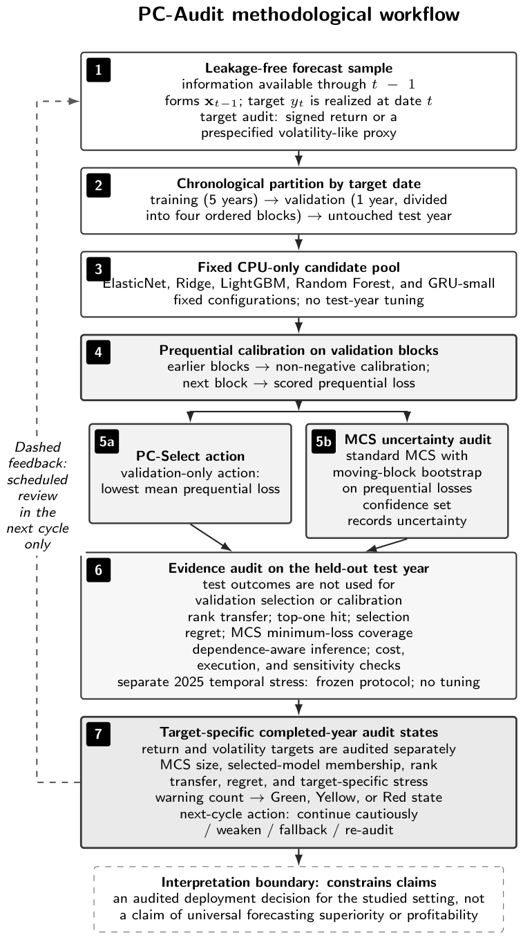
Figure 2.
Signed-return validation-to-test candidate-rank correlations over 45 cases. The prequential mean is positive but small, and its dependence-aware intervals include zero.
Figure 2.
Signed-return validation-to-test candidate-rank correlations over 45 cases. The prequential mean is positive but small, and its dependence-aware intervals include zero.
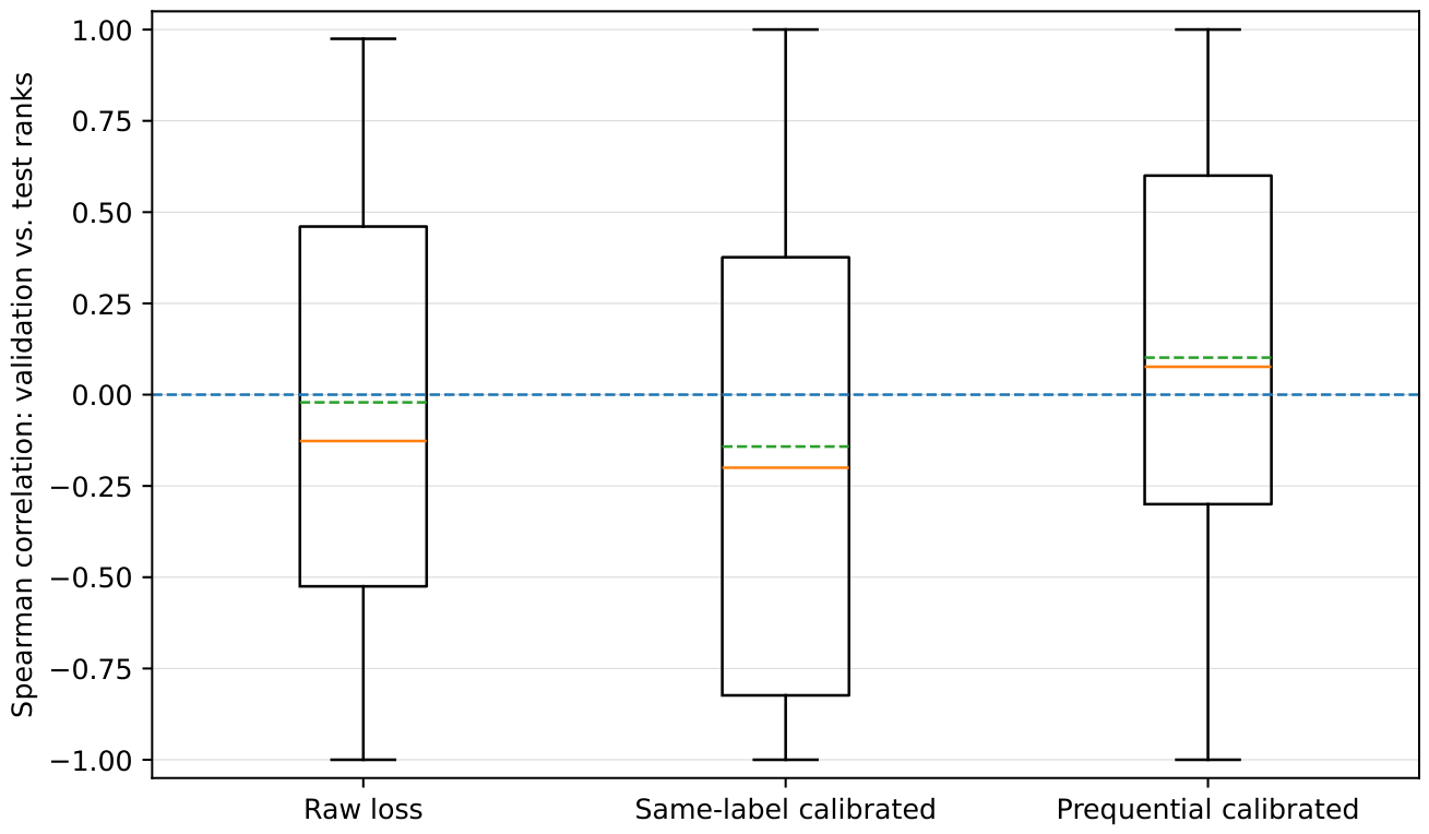
Figure 3.
Distribution of the signed-return prequential validation MAE margin between the first- and second-ranked candidates in the 45 main ETF-window cases. Small margins indicate that many deployment choices are made among nearly tied validation candidates.
Figure 3.
Distribution of the signed-return prequential validation MAE margin between the first- and second-ranked candidates in the 45 main ETF-window cases. Small margins indicate that many deployment choices are made among nearly tied validation candidates.
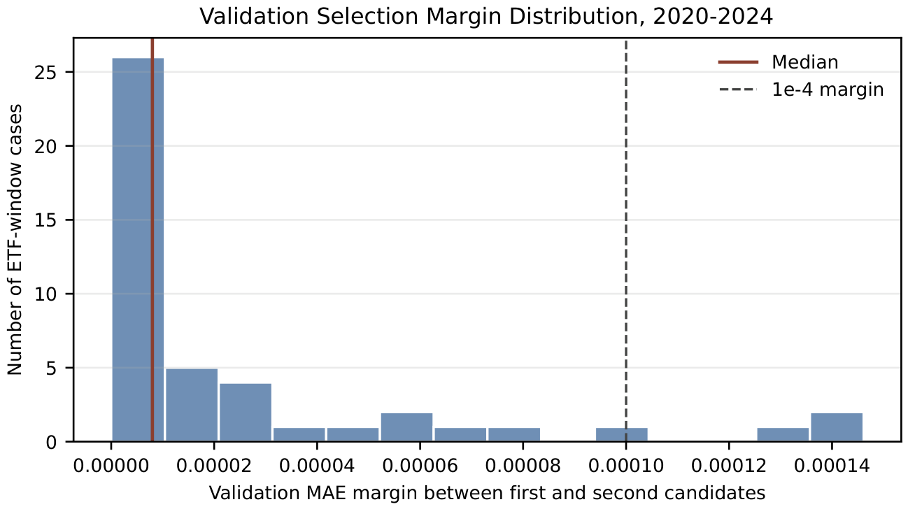

Table 1.
Audit components and their corresponding risk-control objectives.
| Evaluation risk | Protocol response | Interpretation consequence |
|---|---|---|
| Target leakage from next-day returns | Split membership is assigned by target date, not feature-row date | Train, validation, test, and 2025 stress outcomes are chronologically separated |
| Optimistic calibration | Every scored validation block uses a coefficient fitted only on earlier validation blocks | Validation losses used for selection do not reuse the same labels for fitting and scoring |
| Overreading a validation winner | PC-Select is reported with MCS size, candidate-pool minimum coverage, rank transfer, and regret | A single selected model is an action, not proof of statistical separation |
| Multiple testing and dependence | Holm-adjusted tests are supplemented with ETF-cluster and year-block intervals | Positive claims require both multiplicity-adjusted and dependence-aware support |
| Trading-performance overclaiming | Cost, turnover, one-day execution delay, sensitivity variants, and 2025 stress results are reported | Economic metrics are interpreted as diagnostics unless signs remain consistent |
Table 2.
ETF universe. The exact files and SHA-256 hashes are supplied in the reproduction package.
| Ticker | Descriptive fund identifier | Main exposure | Exchange | Rows |
|---|---|---|---|---|
| 510050.SS | SSE 50 ETF | Large-cap SSE 50 | Shanghai | 2916 |
| 510300.SS | CSI 300 ETF | Broad large-cap CSI 300 | Shanghai | 2916 |
| 510500.SS | CSI 500 ETF | Mid/small-cap CSI 500 | Shanghai | 2916 |
| 159915.SZ | ChiNext ETF | ChiNext growth board | Shenzhen | 2916 |
| 159902.SZ | SME 100 ETF | SME 100 | Shenzhen | 2916 |
| 510880.SS | SSE Dividend ETF | Dividend style | Shanghai | 2916 |
| 159928.SZ | CSI Consumer Staples ETF | Consumer staples | Shenzhen | 2916 |
| 159929.SZ | CSI Medical and Health ETF | Health care | Shenzhen | 2916 |
| 159901.SZ | SZSE 100 ETF | SZSE 100 | Shenzhen | 2916 |
Table 3.
Signed-return prediction and directional summaries at 0 bps, averaged over 45 ETF-window cases. Individual candidates use full-validation non-negative calibration before test prediction. DA denotes directional accuracy; BA denotes balanced accuracy. Economic stress values are omitted from the main table and reported in the reproduction package listed in Supplementary Table S1.
Table 3.
Signed-return prediction and directional summaries at 0 bps, averaged over 45 ETF-window cases. Individual candidates use full-validation non-negative calibration before test prediction. DA denotes directional accuracy; BA denotes balanced accuracy. Economic stress values are omitted from the main table and reported in the reproduction package listed in Supplementary Table S1.
| Method | RMSE | MAE | DA | BA | MCC |
|---|---|---|---|---|---|
| Historical mean | 0.015806 | 0.010546 | 0.5316 | 0.5000 | 0.0000 |
| Zero return | 0.015798 | 0.010563 | 0.5181 | 0.5000 | 0.0000 |
| Calibrated ElasticNet | 0.015901 | 0.010654 | 0.5115 | 0.5015 | 0.0022 |
| Calibrated Ridge | 0.015887 | 0.010648 | 0.5065 | 0.4965 | -0.0072 |
| Calibrated LightGBM | 0.015977 | 0.010694 | 0.5094 | 0.4953 | -0.0097 |
| Calibrated Random Forest | 0.015829 | 0.010598 | 0.5207 | 0.4985 | -0.0045 |
| Calibrated GRU-small | 0.015809 | 0.010568 | 0.5059 | 0.4984 | -0.0030 |
| Ensemble Average | 0.016269 | 0.010965 | 0.4929 | 0.4933 | -0.0133 |
| Raw-loss MCS selector | 0.015823 | 0.010603 | 0.5082 | 0.4964 | -0.0097 |
| Same-label calibrated selector | 0.015881 | 0.010650 | 0.5116 | 0.4973 | -0.0062 |
| PC-Select | 0.015821 | 0.010593 | 0.5169 | 0.5000 | -0.0006 |
| MCS equal weight | 0.015840 | 0.010603 | 0.5007 | 0.4932 | -0.0141 |
Table 4.
Signed-return validation-to-test transfer. Relative regret is measured against the best calibrated candidate in each test case. The exact p column is a descriptive uniform-reference diagnostic; the more conservative permutation checks are reported in the text and in the reproduction package listed in Supplementary Table S1.
Table 4.
Signed-return validation-to-test transfer. Relative regret is measured against the best calibrated candidate in each test case. The exact p column is a descriptive uniform-reference diagnostic; the more conservative permutation checks are reported in the text and in the reproduction package listed in Supplementary Table S1.
| Period and protocol | Mean rank |
Top-one hit |
Exact p vs. 0.20 |
MCS minimum coverage |
Mean regret |
Relative regret (%) |
|---|---|---|---|---|---|---|
| 2020–2024 raw loss | -0.019 | 0.156 | 0.577 | 0.644 | 0.000049 | 0.431 |
| 2020–2024 same-label calibrated | -0.126 | 0.356 | 0.014 | 1.000 | 0.000096 | 0.740 |
| 2020–2024 prequential calibrated | 0.090 | 0.333 | 0.038 | 0.933 | 0.000039 | 0.329 |
| 2025 raw loss | -0.242 | 0.222 | 1.000 | 0.667 | 0.000446 | 4.033 |
| 2025 same-label calibrated | 0.426 | 0.444 | 0.086 | 1.000 | 0.000044 | 0.652 |
| 2025 prequential calibrated | 0.220 | 0.222 | 1.000 | 0.889 | 0.000031 | 0.379 |
Table 5.
Effect of calibration timing on signed-return MCS composition and selection. Sel. change is the selected-model change rate relative to PC; set change is the MCS membership-change rate relative to PC. The selectivity–coverage plot is reported in Supplementary Figure S1.
Table 5.
Effect of calibration timing on signed-return MCS composition and selection. Sel. change is the selected-model change rate relative to PC; set change is the MCS membership-change rate relative to PC. The selectivity–coverage plot is reported in Supplementary Figure S1.
| Protocol | Size | All-five | Sel. change | Set change | Min. cov. |
|---|---|---|---|---|---|
| Raw loss | 3.667 | 0.000 | 0.622 | 0.956 | 0.644 |
| Same-label | 4.978 | 0.978 | 0.511 | 0.178 | 1.000 |
| Prequential | 4.800 | 0.844 | – | – | 0.933 |
Table 6.
Validation-reliability comparison across signed-return and volatility-like targets. Volatility-like targets are evaluated only through prediction-scale and validation-transfer diagnostics; they are not used for directional or trading-return claims.
Table 6.
Validation-reliability comparison across signed-return and volatility-like targets. Volatility-like targets are evaluated only through prediction-scale and validation-transfer diagnostics; they are not used for directional or trading-return claims.
| Target | Main rank |
Mean MCS size |
Top-one hit |
2025 rank |
Interpretation |
|---|---|---|---|---|---|
| Signed return | 0.090 | 4.80 | 0.333 | 0.220 | Weak deployment interpretation |
| Absolute return | 0.560 | 3.73 | 0.356 | -0.056 | More auditable, stress-sensitive |
| Squared return | 0.400 | 3.76 | 0.578 | 0.178 | Supports volatility-like robustness |
| Range proxy | 0.631 | 3.38 | 0.178 | 0.078 | Strongest rank-transfer evidence, low top-one hit |
Table 7.
Absolute-return volatility-proxy comparison with stronger naive volatility references, 2020–2024. Positive improvement means lower MAE for PC-Select than for the reference. Naive-Select chooses among Roll-10, Roll-21, Roll-63, EWMA(0.94), and EWMA(0.97) using only the validation year. The signed-rank test reflects paired case-level differences and can be significant even when the mean percentage improvement is small.
Table 7.
Absolute-return volatility-proxy comparison with stronger naive volatility references, 2020–2024. Positive improvement means lower MAE for PC-Select than for the reference. Naive-Select chooses among Roll-10, Roll-21, Roll-63, EWMA(0.94), and EWMA(0.97) using only the validation year. The signed-rank test reflects paired case-level differences and can be significant even when the mean percentage improvement is small.
| Reference | Reference MAE |
PC-Select improvement (%) |
PC better cases |
Holm-adjusted Wilcoxon p |
|---|---|---|---|---|
| Zero proxy | 0.010563 | 31.87 | 44/45 | |
| Historical mean | 0.007392 | 3.75 | 34/45 | 0.0038 |
| Roll-10 | 0.007367 | 0.76 | 33/45 | 0.0041 |
| Roll-21 | 0.007327 | 0.00 | 32/45 | 0.0392 |
| Roll-63 | 0.007360 | 0.52 | 32/45 | 0.0161 |
| EWMA(0.94) | 0.007202 | -1.46 | 29/45 | 0.2456 |
| EWMA(0.97) | 0.007187 | -1.54 | 28/45 | 0.2456 |
| Naive-Select | 0.007279 | -0.54 | 30/45 | 0.0710 |
Table 8.
Signed-return 2025 temporal stress evaluation using the unlagged diagnostic. Stress signs summarize the annual signal-return proxy at 0 and 5 bps; full return and Sharpe values are reported in the accompanying reproduction package.
Table 8.
Signed-return 2025 temporal stress evaluation using the unlagged diagnostic. Stress signs summarize the annual signal-return proxy at 0 and 5 bps; full return and Sharpe values are reported in the accompanying reproduction package.
| Method | RMSE | MAE | BA | MCC | Stress sign 0 bps |
Stress sign 5 bps |
|---|---|---|---|---|---|---|
| Historical mean | 0.011512 | 0.008132 | 0.5000 | 0.0000 | + | + |
| Zero return | 0.011533 | 0.008158 | 0.5000 | 0.0000 | 0 | 0 |
| Ensemble Average | 0.011763 | 0.008388 | 0.4968 | -0.0063 | − | − |
| Raw-loss MCS selector | 0.012146 | 0.008591 | 0.4965 | -0.0083 | + | − |
| Same-label calibrated selector | 0.011572 | 0.008188 | 0.5038 | 0.0095 | + | − |
| PC-Select | 0.011565 | 0.008175 | 0.5039 | 0.0082 | + | − |
| MCS equal weight | 0.011624 | 0.008234 | 0.4984 | -0.0026 | − | − |
Table 9.
Deployment-cycle audit-state and audit-triggered fallback simulation. Panel A reports signed-return annual outputs; mean rank is the case-level validation-to-test candidate-rank correlation averaged within a test year, and mean regret is selected-model test MAE minus the candidate-pool minimum test MAE. Panel B starts in 2021 because the 2020 action has no previous completed audit state; each target uses its own completed-year audit state, and negative worst-year change means lower worst-year MAE under the fallback rule.
Table 9.
Deployment-cycle audit-state and audit-triggered fallback simulation. Panel A reports signed-return annual outputs; mean rank is the case-level validation-to-test candidate-rank correlation averaged within a test year, and mean regret is selected-model test MAE minus the candidate-pool minimum test MAE. Panel B starts in 2021 because the 2020 action has no previous completed audit state; each target uses its own completed-year audit state, and negative worst-year change means lower worst-year MAE under the fallback rule.
| Panel A: Completed-year audit states | |||||||
|---|---|---|---|---|---|---|---|
| Completed test year |
Cases | Mean MCS size |
All-five rate |
Mean rank |
Mean regret |
20 bps stress |
Next-review state and warnings |
| 2020 | 9 | 4.67 | 0.78 | 0.322 | 0.000050 | -0.03547 | Red: large MCS, regret above tolerance, stress nonpositive |
| 2021 | 9 | 5.00 | 1.00 | 0.207 | 0.000045 | -0.08584 | Yellow: large MCS, stress nonpositive |
| 2022 | 9 | 4.56 | 0.67 | -0.113 | 0.000008 | -0.00507 | Red: large MCS, nonpositive rank transfer, stress nonpositive |
| 2023 | 9 | 4.89 | 0.89 | 0.270 | 0.000006 | -0.04131 | Yellow: large MCS, stress nonpositive |
| 2024 | 9 | 4.89 | 0.89 | -0.185 | 0.000086 | 0.00461 | Red: large MCS, nonpositive rank transfer, regret above tolerance |
| Panel B: Next-year fallback simulation | |||||||
| Target | Cases | Blind PC MAE |
Fallback MAE |
Mean change (%) |
Fallback better cases |
Worst-year change (%) |
|
| Signed return | 36 | 0.010248 | 0.010251 | 0.024 | 13/36 | -0.35 | |
| Volatility proxy | 36 | 0.007050 | 0.007087 | 0.517 | 13/36 | -0.90 | |
Table 10.
Unaudited validation interpretation versus PC-Audit interpretation.
| Evidence item | Possible unaudited interpretation | PC-Audit interpretation |
|---|---|---|
| Lowest prequential validation MAE | Select and deploy the validation winner as the preferred model | Selection is allowed as an action, but its interpretation depends on uncertainty and transfer diagnostics |
| PC-Select top-one hit rate of 15/45 | Treat the hit rate as evidence that validation selection beats a random five-model choice | Borderline only; the global label-permutation diagnostic gives |
| Mean prequential MCS size of 4.80/5 | Ignore confidence-set size and report only the selected model name | Report weak statistical separation because nearly all candidates remain admissible |
| Zero-return and historical-mean references | Treat naive references as trivial checks secondary to the selected model | No significant lower-error advantage over naive references is detected after multiplicity adjustment |
| Validation reliability across targets | Treat the absolute-return result as proof that PC-Select is a superior volatility model | Report the target-level result: volatility-like targets transfer better than signed returns, while rolling and EWMA references remain competitive |
| Cost, execution, and 2025 stress signs | Report favorable gross diagnostics as economic evidence | Do not claim investable evidence because signs change under costs, execution modes, sensitivity variants, and temporal stress |
| Completed annual audit states | Carry the latest validation winner into the next review without qualification | Carry forward Green/Yellow/Red states; fallback can modestly reduce worst-year risk but is not an average-accuracy improvement rule |
Disclaimer/Publisher’s Note: The statements, opinions and data contained in all publications are solely those of the individual author(s) and contributor(s) and not of MDPI and/or the editor(s). MDPI and/or the editor(s) disclaim responsibility for any injury to people or property resulting from any ideas, methods, instructions or products referred to in the content. |
© 2026 by the authors. Licensee MDPI, Basel, Switzerland. This article is an open access article distributed under the terms and conditions of the Creative Commons Attribution (CC BY) license.
Copyright: This open access article is published under a Creative Commons CC BY 4.0 license, which permit the free download, distribution, and reuse, provided that the author and preprint are cited in any reuse.