A Pure Geometric Foundation of Mathematics from the Non-Proper Archimedean Conical Helix

1. Introduction

The question of whether a substantial body of mathematics can be generated from a single geometric primitive, without prior appeal to numbers, sets, or analytic structure, has a long history [1,2,3,4,5]. Classical Euclidean geometry begins with points, lines, and planes taken as undefined terms [5,6,7,8], while modern foundational programs typically begin with logic or set theory [2,3,9]. In the present work a different route is explored: Taken as primitive a single geometric object—the non-proper Archimedean conical helix [10,11]—together with a small collection of purely geometric operations (continuous coiling, chiral twist, orthogonal projection, radial growth, non-terminating extension, cycle decomposition [12,13,14], and flux [15]), and three axioms that encode maximal cohesive spread, persistent ground twist, and indecomposable flux conservation [15,16,17,18].

From this minimal geometric starting point reconstructing, in successive stages, the classical Euclidean toolkit [5,6,7,19], the fundamental mathematical constants [10,20,21,22], geometric arithmetic and induction, the full calculus pipeline [13,23,24,25,26,27], real and complex analysis [28,29], measure theory [30,31,32], and the principal structures of differential geometry [11,33,34,35,36]. The development is strictly constructive: each new notion is introduced only after the geometric tools required for its definition have already been secured [9,16,18]. The paper culminates in a pure geometric account of sets and functions [2,37] and in the observation that the same helix simultaneously exhibits a continuous (wave-like) aspect and a discrete (particle-like) aspect [11,38,39].

The scope of the present paper is deliberately limited. Stopping at the geometric form of wave–particle duality. The further passage from this pure geometric setting to a cohesive topos, an internal homotopy type theory, and a Boolean reflection yielding ZFC is left for subsequent work [4,37,40,41]. The aim here is simply to show that a single, carefully chosen geometric figure, governed by three transparent geometric principles, is already rich enough to generate a large and coherent fragment of classical mathematics [4,7].

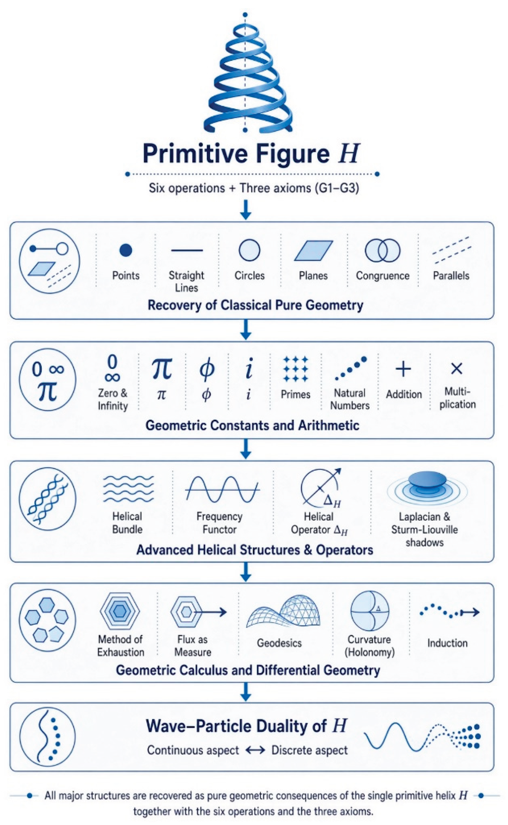
The remainder of the paper is organized as follows. Section 2 introduces the primitive helix, the six operations, and the three axioms, and establishes uniqueness. Section 3, Section 4 and Section 5 recover classical Euclidean geometry [5,6,7,8,49], the notions of zero and infinity, and geometric arithmetic. Section 6, Section 7 and Section 8 develop the fundamental constants, the advanced helical structures [11,39,54], and the precursors of the calculus [13,14,23,24,25,26,27,41,44]. Section 9, Section 10, Section 11 and Section 12 present the full pure-geometric calculus, analysis, and differential geometry [29,31,33,34,35,36,46,47,48]. The final section treats geometric sets, geometric functions, and the wave–particle duality inherent in the helix [2,11,37].

Figure 1. Cascade Overview – From the Primitive Helix $H$ to the Recovered Structures.

Figure 1. Cascade Overview – From the Primitive Helix $H$ to the Recovered Structures.

2. Primitive Foundation

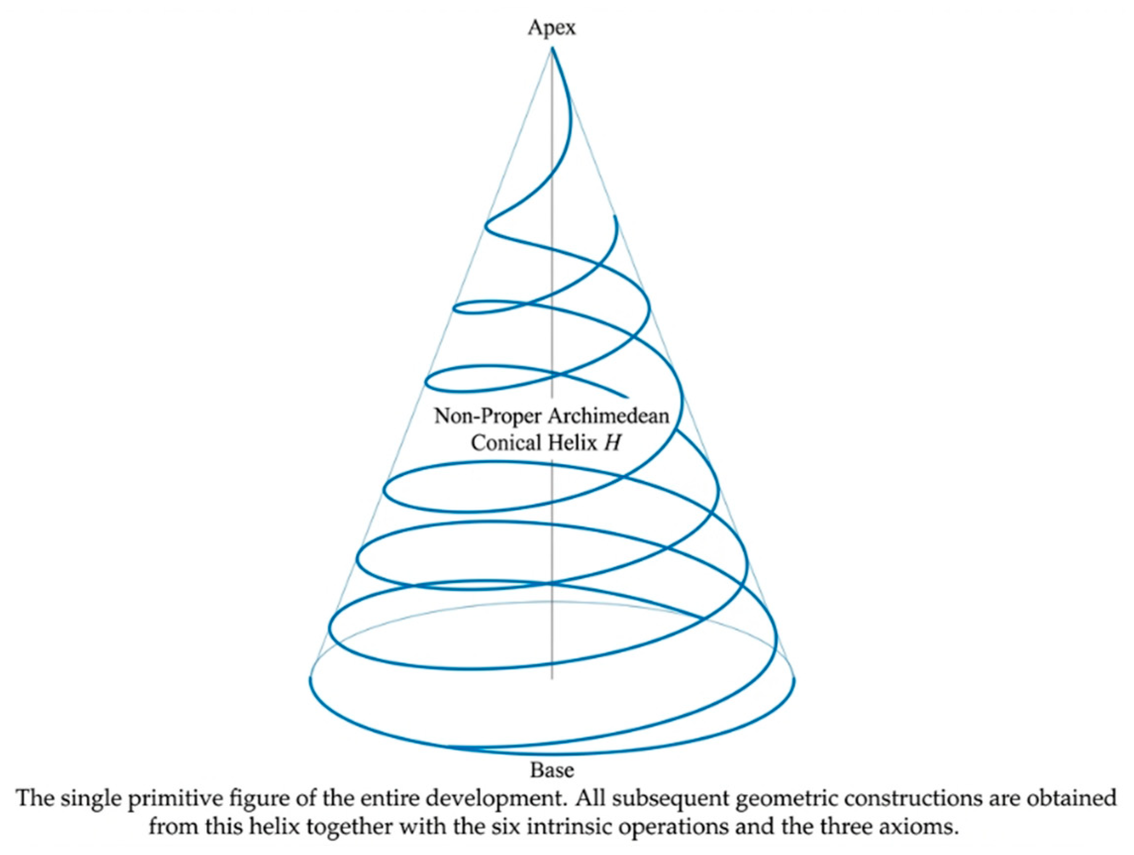
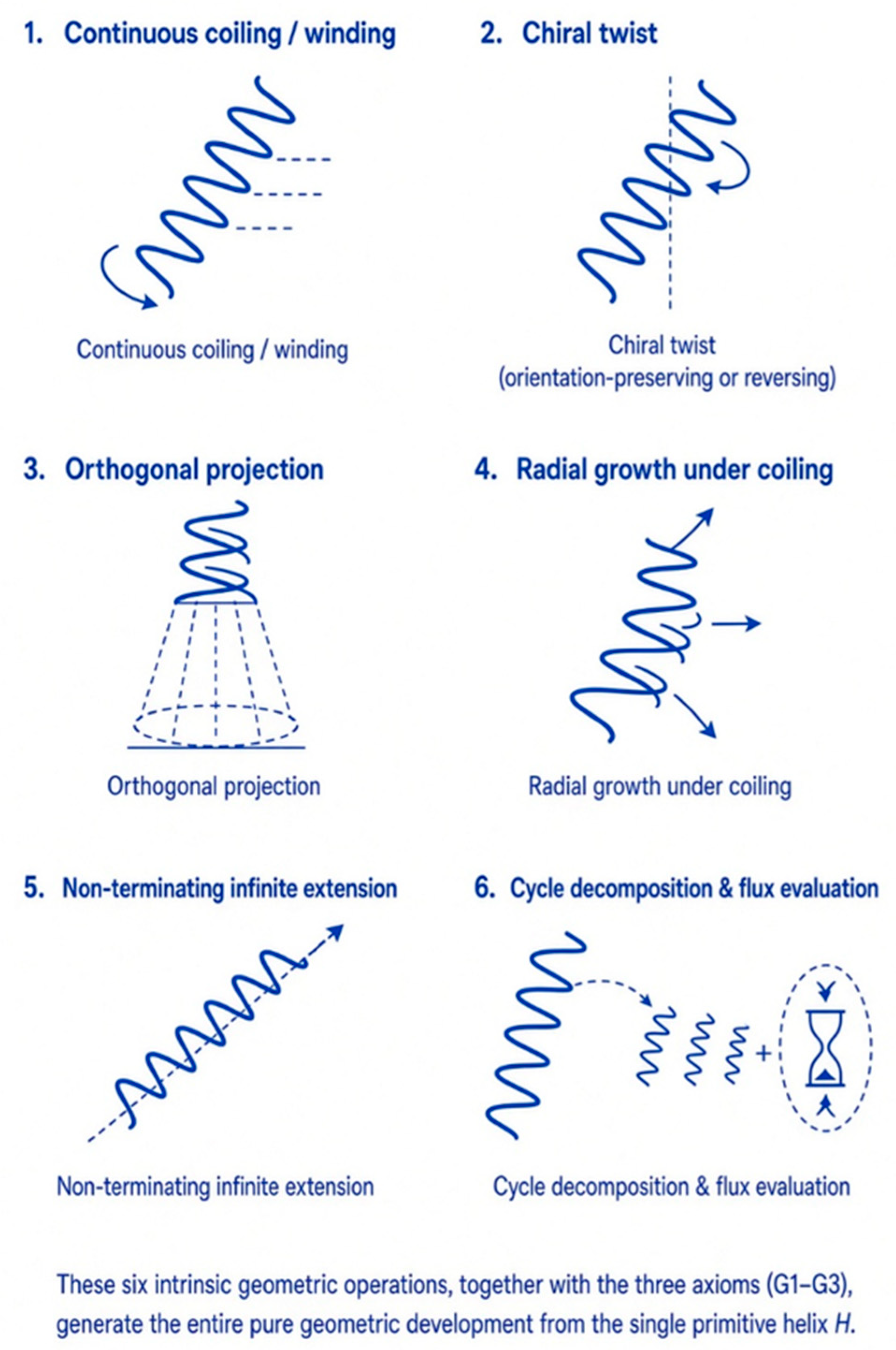
A single geometric figure is taken as primitive: the non-proper Archimedean conical helix [10,11]. This figure is equipped with six intrinsic geometric operations—continuous coiling, chiral twist, orthogonal projection, radial growth, non-terminating extension, and cycle decomposition [11,12,13]—together with the observable quantity of flux [15]. Three geometric axioms are imposed upon these operations [16,18]. The first axiom requires maximal cohesive spread under continuous coiling and radial growth [4,37]. The second axiom requires the persistence of a non-vanishing ground twist under every admissible transformation [11]. The third axiom requires the indecomposable conservation of flux [15,32]. From these data the uniqueness of the primitive figure, up to unique geometric isomorphism, is established [6,7]. All subsequent constructions of the present work are obtained exclusively as geometric consequences of this single figure, its six operations, and the three axioms.

Theorem 1 (Pure Geometric Foundation of Mathematics). There exists a unique (up to unique isomorphism) pregeometry $P_H$ generated by the single primitive figure — the non-proper Archimedean conical helix $H$ — together with six purely geometric construction operations [9,40]. The unique universal functor associated to$P_H$ generates the sheaf topos$Sh\left(P_H\right)$ [4,37,40] whose internal type theory is homotopy type theory (HoTT) with univalence, and whose Boolean reflection satisfies ZFC [2,37,40]. All downstream structures are recovered as canonical shadows of this geometry [4]. The entire construction is free of circular reasoning and uses only the primitive figure$H$, the six operations, and the three axioms G1–G3 [8,10,49].

2.1. Primitive Signature

The pregeometry $P_H$ is the free syntactic category generated by [2,17,41]:

• One object: the primitive figure $H$ (the non-proper Archimedean conical helix) [10,11].
• Six primitive operation symbols (geometric constructors) [12]:

  ○

  $\mathrm{C}\mathrm{o}\mathrm{i}\mathrm{l}:H\to H$ (continuous coiling / winding) [11],

  ○

  $\mathrm{T}\mathrm{w}\mathrm{i}\mathrm{s}\mathrm{t}:H\to H$ (chiral twist — orientation-preserving or reversing) [11,33],

  ○

  $\mathrm{P}\mathrm{r}\mathrm{o}\mathrm{j}\mathrm{e}\mathrm{c}\mathrm{t}:H\to H$ (orthogonal projection) [11,49],

  ○

  $\mathrm{G}\mathrm{r}\mathrm{o}\mathrm{w}:H\to H$ (radial growth under coiling) [11],

  ○

  $\mathrm{E}\mathrm{x}\mathrm{t}\mathrm{e}\mathrm{n}\mathrm{d}:H\to H$ (non-terminating infinite extension) [6,30],

  ○

  $\mathrm{D}\mathrm{e}\mathrm{c}\mathrm{o}\mathrm{m}\mathrm{p}\mathrm{o}\mathrm{s}\mathrm{e}:H\to H$ (cycle formation and indivisible minimal-cycle decomposition) [13,14,32],

  ○

  $\mathrm{F}\mathrm{l}\mathrm{u}\mathrm{x}:H\to H$(observable total crossing count) [15,28].

Morphisms in $P_H$ are finite compositions of these operations (and their inverses where the axioms allow). Composition is associative and unital; identities are the trivial applications. No other objects or morphisms exist [3,9].

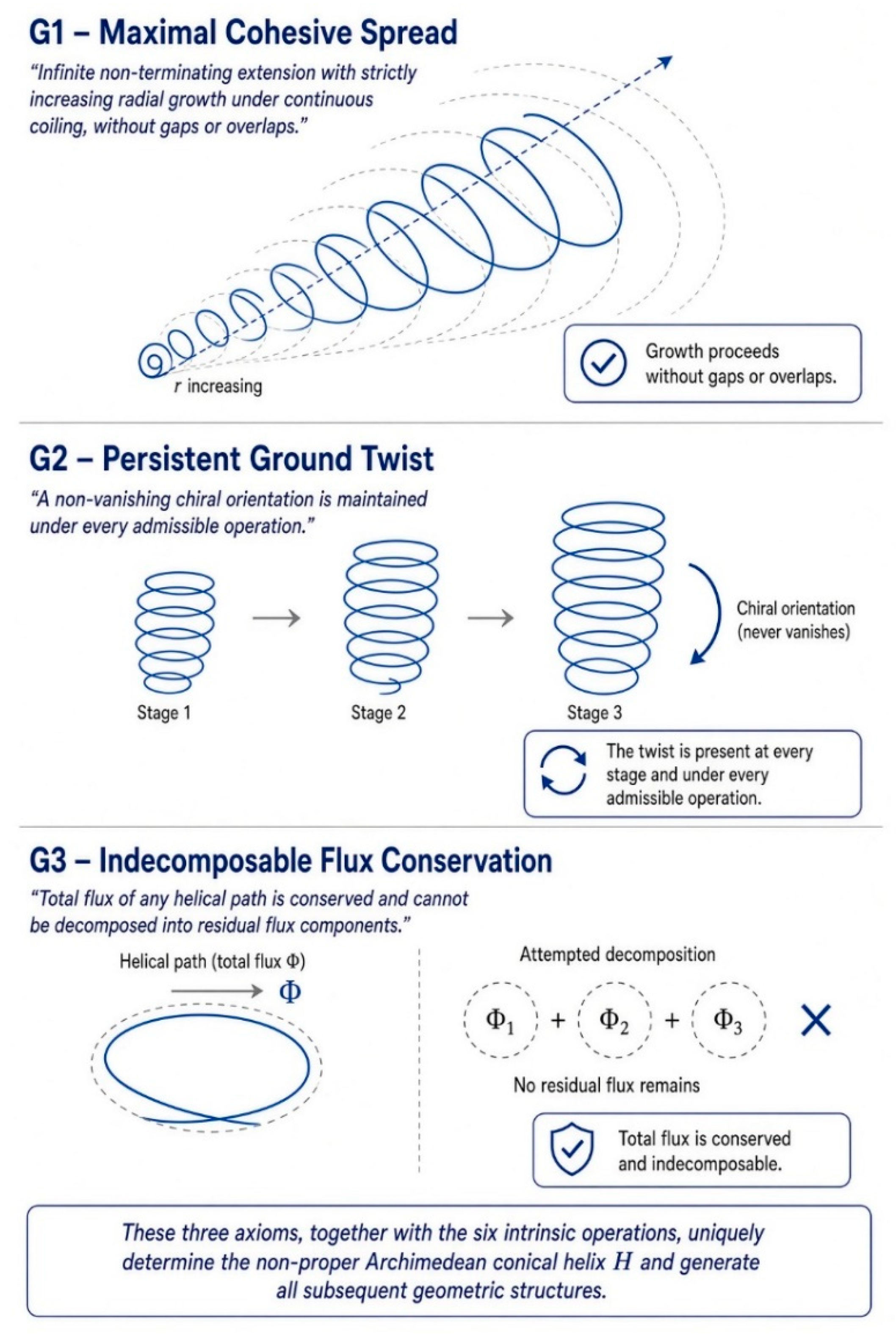
2.2. The Three Pure Geometric Axioms (Construction Rules – as Geometric Sequents) [9,16,17,18]

2.2.1. Axiom G1 (Maximal Cohesive Spread)

$\forall x\left(\mathrm{E}\mathrm{x}\mathrm{t}\mathrm{e}\mathrm{n}\mathrm{d}\right(x)\wedge \mathrm{G}\mathrm{r}\mathrm{o}\mathrm{w}(\mathrm{C}\mathrm{o}\mathrm{i}\mathrm{l}\left(x\right))⊢\neg \mathrm{T}\mathrm{e}\mathrm{r}\mathrm{m}\mathrm{i}\mathrm{n}\mathrm{a}\mathrm{l}(x\left)\right)$ [16,18]

Any sequence forcing terminal closure or constant radial width collapses $H$ (via $\mathrm{P}\mathrm{r}\mathrm{o}\mathrm{j}\mathrm{e}\mathrm{c}\mathrm{t}$then $\mathrm{D}\mathrm{e}\mathrm{c}\mathrm{o}\mathrm{m}\mathrm{p}\mathrm{o}\mathrm{s}\mathrm{e}$) to a lower-dimensional non-chiral sub-figure [7,11,42].

2.2.2. Axiom G2 (Persistent Ground Twist)

$\forall x\left(\mathrm{P}\mathrm{r}\mathrm{o}\mathrm{j}\mathrm{e}\mathrm{c}\mathrm{t}\right(x)⊢\exists !t:\mathrm{T}\mathrm{w}\mathrm{i}\mathrm{s}\mathrm{t}(x\left)\mathrm{such}\mathrm{that}\mathrm{F}\mathrm{l}\mathrm{u}\mathrm{x}\right(t)\ne 0)$ [11,15]

There exists no projection sequence that flattens $H$ to a zero-twist degenerate sub-figure [11,19].

Figure 2. The Non-Proper Archimedean Conical Helix $H$ (Primitive Figure).

Figure 2. The Non-Proper Archimedean Conical Helix $H$ (Primitive Figure).

2.2.3. Axiom G3 (Indecomposable Flux Conservation)

$\forall x\left(\mathrm{D}\mathrm{e}\mathrm{c}\mathrm{o}\mathrm{m}\mathrm{p}\mathrm{o}\mathrm{s}\mathrm{e}\right(x)⊢\mathrm{the}\mathrm{resulting}\mathrm{cycles}\mathrm{are}\mathrm{indecomposable}\mathrm{and}\mathrm{F}\mathrm{l}\mathrm{u}\mathrm{x}\mathrm{is}\mathrm{preserved})$ [13,15,32]

$H$ cannot be decomposed into two or more independent sub-helices while preserving total winding flux [11,15].

These sequents are the only relations imposed on the free category $P_H$ [9,16].

Figure 3. The Six Intrinsic Operations of the Primitive Helix $H.$

Figure 3. The Six Intrinsic Operations of the Primitive Helix $H.$

2.3. Uniqueness

Theorem 2 (Uniqueness of$H$). Up to unique isomorphism in $P_H$, the non-proper Archimedean conical helix $H$ is the sole figure satisfying Geometric Axioms G1–G3 [1,6,7]. Any other candidate figure fails at least one axiom by direct geometric collapse or decomposition [19,42].

Proof of Theorem 2.

Step 1 (Generation of $P_H$)

$P_H$ is the free syntactic category on $H$ and the six operation symbols [3,9]. Morphisms are finite words in the operation symbols, subject only to the equalities forced by the sequents G1–G3 [16,18].

Step 2 (Verification of G1 – Maximal Cohesive Spread)

Apply $\mathrm{E}\mathrm{x}\mathrm{t}\mathrm{e}\mathrm{n}\mathrm{d}$ repeatedly: each step produces a longer helical segment. Compose with $\mathrm{C}\mathrm{o}\mathrm{i}\mathrm{l}$ and $\mathrm{G}\mathrm{r}\mathrm{o}\mathrm{w}$: radial distance strictly increases [11]. Suppose a sequence forces terminal closure or constant radial width. Apply the concrete sequence [7,11]

$$\mathrm{P}\mathrm{r}\mathrm{o}\mathrm{j}\mathrm{e}\mathrm{c}\mathrm{t}\circ \mathrm{D}\mathrm{e}\mathrm{c}\mathrm{o}\mathrm{m}\mathrm{p}\mathrm{o}\mathrm{s}\mathrm{e}\circ \mathrm{T}\mathrm{w}\mathrm{i}\mathrm{s}\mathrm{t}$$

This yields a lower-dimensional non-chiral sub-figure, contradicting G1. Hence $H$ satisfies maximal cohesive spread.

Step 3 (Verification of G2 – Persistent Ground Twist)

Apply $\mathrm{P}\mathrm{r}\mathrm{o}\mathrm{j}\mathrm{e}\mathrm{c}\mathrm{t}$: the resulting diagram admits a unique chiral ground twist via $\mathrm{T}\mathrm{w}\mathrm{i}\mathrm{s}\mathrm{t}$. Suppose a projection sequence flattens $H$ to zero twist. Then $\mathrm{F}\mathrm{l}\mathrm{u}\mathrm{x}$ vanishes after finitely many $\mathrm{P}\mathrm{r}\mathrm{o}\mathrm{j}\mathrm{e}\mathrm{c}\mathrm{t}\circ \mathrm{T}\mathrm{w}\mathrm{i}\mathrm{s}\mathrm{t}$ steps, contradicting G2 [15]. Hence every projection preserves non-collapsing chiral ground twist.

Step 4 (Verification of G3 – Indecomposable Flux Conservation + Global Uniqueness)

Suppose $H$ decomposes into independent sub-helices via $\mathrm{D}\mathrm{e}\mathrm{c}\mathrm{o}\mathrm{m}\mathrm{p}\mathrm{o}\mathrm{s}\mathrm{e}$. The concrete sequence

$$\mathrm{D}\mathrm{e}\mathrm{c}\mathrm{o}\mathrm{m}\mathrm{p}\mathrm{o}\mathrm{s}\mathrm{e}\circ \mathrm{F}\mathrm{l}\mathrm{u}\mathrm{x}$$

shows that total winding flux splits, contradicting preservation of $\mathrm{F}\mathrm{l}\mathrm{u}\mathrm{x}$ under G3 [15,32]. Every cycle is indecomposable (no further non-trivial splitting preserves $\mathrm{F}\mathrm{l}\mathrm{u}\mathrm{x}$) [13,32].

Now let $H^{\prime }$ be any other figure satisfying G1–G3. Apply the matching sequence of operations used on $H$:

• $\mathrm{E}\mathrm{x}\mathrm{t}\mathrm{e}\mathrm{n}\mathrm{d}\circ \mathrm{C}\mathrm{o}\mathrm{i}\mathrm{l}\circ \mathrm{G}\mathrm{r}\mathrm{o}\mathrm{w}$ forces infinite extension with increasing radial growth (G1) [11].
• $\mathrm{P}\mathrm{r}\mathrm{o}\mathrm{j}\mathrm{e}\mathrm{c}\mathrm{t}\circ \mathrm{T}\mathrm{w}\mathrm{i}\mathrm{s}\mathrm{t}$ preserves chiral twist (G2) [11].
• $\mathrm{D}\mathrm{e}\mathrm{c}\mathrm{o}\mathrm{m}\mathrm{p}\mathrm{o}\mathrm{s}\mathrm{e}\circ \mathrm{F}\mathrm{l}\mathrm{u}\mathrm{x}$ forces indecomposability (G3) [15].

Any deviation produces a collapse (terminal closure via $\mathrm{P}\mathrm{r}\mathrm{o}\mathrm{j}\mathrm{e}\mathrm{c}\mathrm{t}\circ \mathrm{D}\mathrm{e}\mathrm{c}\mathrm{o}\mathrm{m}\mathrm{p}\mathrm{o}\mathrm{s}\mathrm{e}$, zero twist via $\mathrm{P}\mathrm{r}\mathrm{o}\mathrm{j}\mathrm{e}\mathrm{c}\mathrm{t}\circ \mathrm{T}\mathrm{w}\mathrm{i}\mathrm{s}\mathrm{t}$, or flux-splitting via $\mathrm{D}\mathrm{e}\mathrm{c}\mathrm{o}\mathrm{m}\mathrm{p}\mathrm{o}\mathrm{s}\mathrm{e}$) [13,14]. Therefore $H^{\prime }\cong H$ via the unique isomorphism in $P_H$ induced by matching operation sequences (a monomorphism that is injective on Flux and Twist invariants) [9,37].

This completes the proof of Theorem 2 (and thereby the uniqueness clause of Theorem 1).

2.4. Unique Universal Functor

Definition Let $\mathrm{S}\mathrm{h}\left(P_H\right)$ be the sheaf topos on the syntactic category $P_H$ [37,40] equipped with the Grothendieck topology whose covering families are all finite families of morphisms $\left\{f_i:D_i\to H\right\}$ (compositions of $\mathrm{C}\mathrm{o}\mathrm{i}\mathrm{l}$, $\mathrm{P}\mathrm{r}\mathrm{o}\mathrm{j}\mathrm{e}\mathrm{c}\mathrm{t}$, etc.) such that [37,40]:

• their images jointly cover $H$ (every point is reached by some $f_i$),
• the family preserves full flux and maximal spread (G1–G3 hold on the union) [4,15],
• the family is stable under pullback and satisfies transitivity (standard Grothendieck axioms) [37,40].

The unique universal functor is the left adjoint

$$U:P_H⟶\mathrm{S}\mathrm{h}\left(P_H\right)$$

given explicitly by the Yoneda embedding composed with sheafification with respect to the above covering families [37,40]. It satisfies the universal property that $U\left(H\right)$ is the free helical sheaf realizing G1–G3 as natural transformations [4,9].

Figure 4. The Three Geometric Axioms of the Primitive Helix $H.$

Figure 4. The Three Geometric Axioms of the Primitive Helix $H.$

Theorem 3 (Uniqueness of the Universal Functor$U$). Let $Sh\left(P_H\right)$ be the sheaf topos on $P_H$ with the Grothendieck topology defined above [37,40]. Let$U:P_H\to Sh\left(P_H\right)$ be the left adjoint realizing G1–G3 as natural transformations. Because$H$ is the sole figure satisfying G1–G3 (Theorem 2), any functor satisfying the same universal property is canonically naturally isomorphic to$U$ [4,37,40].

Proof of Theorem 3.

Any other functor $U^{\prime }$ must send $H$ to a helical sheaf satisfying G1–G3. By Theorem 2 this sheaf is uniquely isomorphic (in $\mathrm{S}\mathrm{h}\left(P_H\right)$) to $U\left(H\right)$. The isomorphism is natural because both are left adjoints to the same forgetful functor and agree on the generator $H$ [37,40]. □

3. Recovery of Classical Pure Geometry

The classical primitives of Euclidean geometry are recovered as geometric shadows of the non-proper Archimedean conical helix under the six intrinsic operations and the three axioms [5,6,7,11]. Points arise as the unique intersection loci of successive orthogonal projections of helical paths [6,7,11]. Straight lines are obtained as the orthogonal projections of helical paths of vanishing radial growth [6,7]. The recovered plane is generated by unrestricted radial growth under continuous coiling and orthogonal projection [6,7,8]. Incidence, betweenness, and order are induced by membership in projected helical paths and by the axial direction of the helix [6,7,8]. Congruence of segments and angles is realized by flux-preserving compositions of the six operations [6,7,15]. Circles appear as the loci of constant radial flux under continuous coiling [5,10,11]. From these constructions the isosceles-triangle theorem, the full set of triangle-congruence criteria [5,6,7], the construction of parallels with equal alternate interior angles [5,19,42], the existence of intersections [6,7], and the classical ruler-and-compass constructions [5,7,49] are established successively as pure geometric consequences of the helix. No external Euclidean postulates are assumed [6,7].

Figure 5. Orthogonal Projections of the Helical Paths – Origin of Points, Lines, and Circles.

Figure 5. Orthogonal Projections of the Helical Paths – Origin of Points, Lines, and Circles.

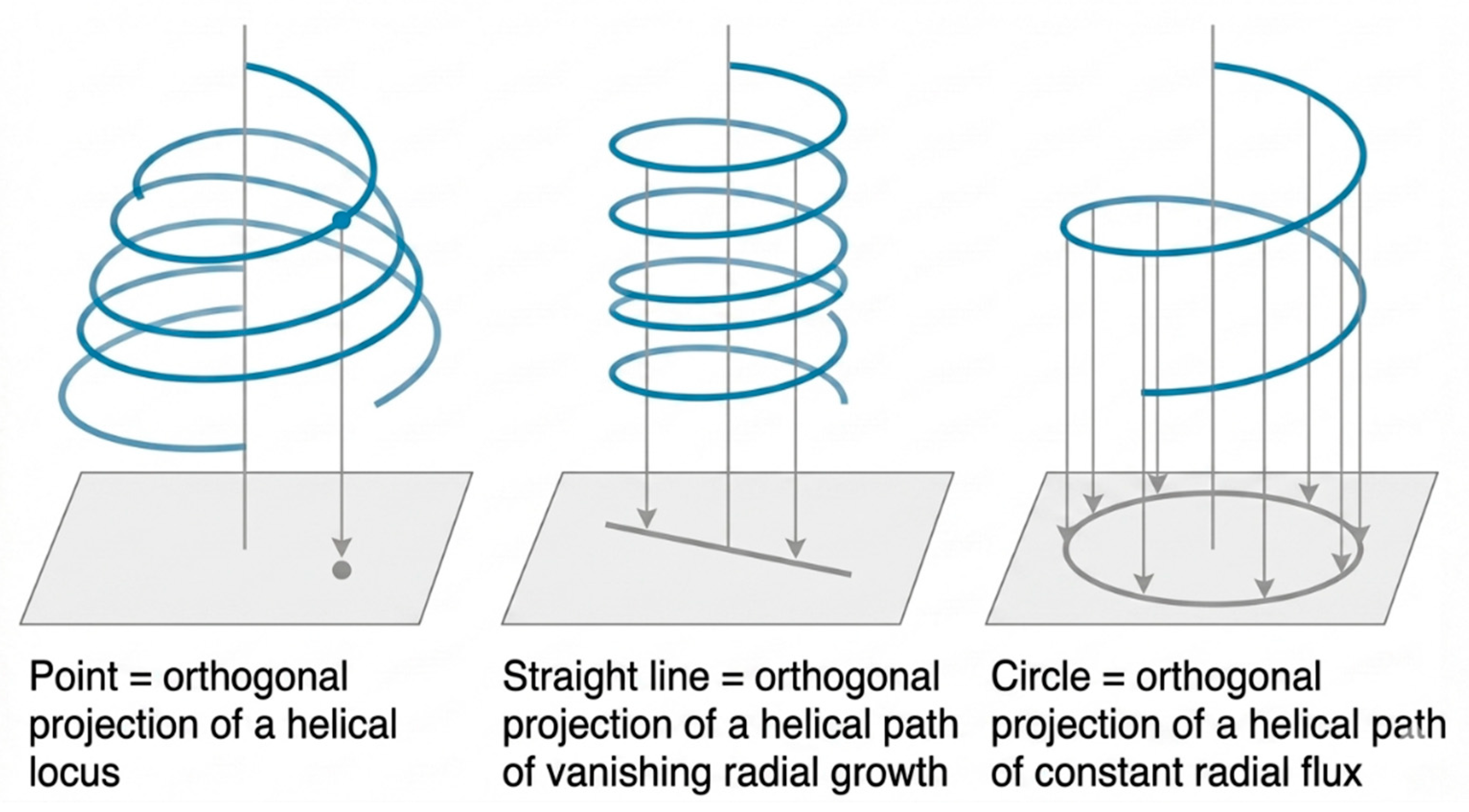
Theorem 4 (Definition of Point). A geometric point is the unique locus obtained as the intersection of successive orthogonal projections of helical paths of $H$ under maximal cohesive spread [6,7,11].

Proof of Theorem 4.

• Apply the continuous coiling operation to $H$ and take successive orthogonal projections (Project operation) [11].
• By G1 (maximal cohesive spread), these projections intersect in a single common locus that cannot be further decomposed [7].
• By G3 (indecomposable flux conservation), this locus carries zero residual flux and is therefore indivisible [13,15].
• The resulting locus is independent of the particular sequence of projections chosen (uniqueness follows from the uniqueness of $H$, Theorem 3) [6].
• This locus is called a geometric point [5,6].

This proves Theorem 4. □

Theorem 5 (Definition of Straight Line). A straight line is the orthogonal projection of a helical path of $H$ in which the radial growth vanishes while the axial extension continues without termination [5,6,11].

Proof of Theorem 5.

• Consider a helical path generated by continuous coiling of $H$ [11].

2.

Apply the Grow operation with radial increment set to zero while retaining non-terminating axial extension (Extend operation) [11].

3.

The resulting path has vanishing curvature in the radial direction [11].

4.

Its orthogonal projection (Project operation) is a figure that admits no further radial deviation under any composition of the six operations [11,49].

5.

By G1 and G2, this projected figure is unique up to congruence and is called a straight line [6,7].

This proves Theorem 5. □

Theorem 6 (Definition of Plane). The recovered plane is the unique surface generated by the continuous radial growth of $H$ under all admissible orthogonal projections that satisfy maximal cohesive spread [6,7,8].

Proof of Theorem 6.

• Apply continuous coiling together with unrestricted radial growth (Grow operation) to $H$ [11].

2.

Take the collection of all orthogonal projections of the resulting paths (Project operation) [11].

3.

By G1 (maximal cohesive spread), these projections fill a unique two-dimensional surface without gaps or overlaps [7,8].

4.

By G3, the total flux on this surface is conserved and indecomposable into higher-dimensional components [15].

5.

This surface is independent of the particular sequence of projections and is called the recovered plane [6,42].

This proves Theorem 6. □

Theorem 7 (Incidence Relation). A point $P$ is incident to a straight line $\mathcal{l}$ (respectively, to the recovered plane) if and only if $P$ belongs to a helical path whose orthogonal projection is $\mathcal{l}$ (respectively, lies entirely within the recovered plane) [5,6,7].

Proof of Theorem 7

• Let $P$ be a geometric point (Theorem 4) and $\mathcal{l}$ a straight line (Theorem 5).
• By construction, $P$ arises as the intersection of projected helical paths [11].
• If there exists a helical path containing the pre-image of $P$ whose orthogonal projection coincides with $\mathcal{l}$, then $P$ lies on $\mathcal{l}$.
• Conversely, if $P$ lies on $\mathcal{l}$, the pre-image helical path projects onto $\mathcal{l}$ by the definition of straight line.
• The same reasoning applied to the recovered plane (Theorem 6) yields the incidence relation between points and the plane [6].
• Incidence is therefore completely determined by the six operations and the axioms.

This proves Theorem 7 [6,7]. □

Theorem 8 (Betweenness and Order). On a straight line $\mathcal{l}$, a point $B$ lies between points $A$ and $C$ if and only if the projected helical path from $A$ to $C$ passes through $B$ under non-terminating axial extension, and the order is the unique order induced by the axial direction of $H$ [6].

Proof of Theorem 8.

• Let $A$, $B$, $C$ be points incident to a straight line $\mathcal{l}$ (Theorems 5 and 7).
• Lift $A$ and $C$ to helical paths of $H$ [11].
• Apply continuous axial extension (Extend operation) connecting the pre-images of $A$ and $C$.
• By G1 and the uniqueness of the axial direction of $H$, there is a unique continuous path on the lift that projects onto the segment of $\mathcal{l}$ between $A$ and $C$ [6,8].
• The point $B$ lies between $A$ and $C$ precisely when its pre-image lies on this unique path [8].
• The resulting betweenness relation is asymmetric, transitive on the line, and independent of the choice of lift [6,7].

This proves Theorem 8. □

Theorem 9 (Congruence of Segments and Angles). Two segments (respectively, two angles) are congruent if and only if there exists a finite composition of the six primitive operations that maps one onto the other while preserving total flux and orientation (up to chiral twist) [6,7,15,49].

Proof of Theorem 9.

• Let $\overline{AB}$ and $\overline{CD}$ be two segments on the recovered plane.
• Lift both segments to helical paths of $H$ [11].
• Apply a finite sequence of Coil, Twist, Project, Grow, and Extend operations that carries the pre-image of $\overline{AB}$ onto the pre-image of $\overline{CD}$ [12].
• By G3 (flux conservation), the total flux of the two segments must be equal [15].
• By G2 (persistent ground twist), orientation is preserved up to a global chiral reversal [11].
• When such a flux-preserving and orientation-preserving composition exists, the segments are declared congruent [6,7].
• The identical construction applied to angles (formed by pairs of intersecting lines) yields congruence of angles [5,6].
• Congruence is an equivalence relation by the composition properties of the six operations [6].

This proves Theorem 9. □

Theorem 10 (Circle). A circle is the locus of all points on the recovered plane obtained by continuous coiling of $H$ about a fixed center point at constant radial distance (constant flux length from the center under orthogonal projection) [5,10,11].

Proof of Theorem 10.

• Fix a geometric point $O$ as center (Theorem 4).
• Apply continuous coiling of $H$ while holding the radial growth parameter constant (Grow operation with fixed increment) [11].
• Take the orthogonal projection of the resulting path (Project operation) [10,11].
• By G1 (maximal cohesive spread), the projected locus is a closed curve consisting of all points at equal flux distance from $O$ [5,7].
• By G3 (flux conservation), this distance is independent of the starting angle of the coil [15].
• The resulting figure is unique up to congruence and is called a circle with center $O$.

This proves Theorem 10 [5,6]. □

Theorem 11 (Isosceles Triangle Theorem – Base Angles Equal). In any triangle formed by three points on the recovered plane in which two sides are congruent, the base angles opposite those sides are congruent [5,7].

Proof of Theorem 11.

• Let $△ABC$ be a triangle in which segments $\overline{AB}$ and $\overline{AC}$ are congruent (Theorem 9) [5].
• Lift the two congruent sides to helical paths of $H$ emanating from the common apex $A$ [11].
• Because the sides are congruent, there exists a flux-preserving composition of the six operations (in particular a chiral Twist or its reverse) that maps the pre-image of $\overline{AB}$ onto the pre-image of $\overline{AC}$ while fixing $A$ [15,49].
• This composition maps the angle at $B$ onto the angle at $C$.
• By Theorem 9, the two base angles are therefore congruent [5].
• The result is independent of the particular lift chosen.

This proves Theorem 11. □

Theorem 12 (Full Triangle Congruence Theorems – ASA, SSS, AAS). Two triangles on the recovered plane are congruent if they satisfy any one of the following criteria [5,7]:

• ASA (two angles and the included side),
• SSS (three sides),
• AAS (two angles and a non-included side).

Proof of Theorem 12.

• Let $△ABC$ and $△DEF$ be two triangles.
• In each case (ASA, SSS, or AAS), the given corresponding sides and/or angles are congruent by hypothesis (Theorem 9) [5].
• Lift both triangles to helical paths of $H$
• Because the corresponding flux lengths (sides) and flux twists (angles) match, there exists a finite composition of Coil, Twist, Project, Grow, and Extend that carries the pre-image of $△ABC$ onto the pre-image of $△DEF$ [7,49].
• This composition preserves total flux (G3) and orientation up to global chirality (G2) [11,15].
• Therefore the triangles are congruent by the definition of congruence (Theorem 9) [6].
• Uniqueness of the mapping follows from the uniqueness of $H$ (Theorem 3) and maximal cohesive spread (G1).

This proves Theorem 12. □

Theorem 13 (Parallel Construction and Alternate Interior Angles Theorem). Two distinct straight lines on the recovered plane are parallel if and only if a transversal forms congruent alternate interior angles with them [5,19,42]. Moreover, such parallel lines can be constructed by projecting helical paths that share the same axial direction and the same persistent ground twist [7,11].

Proof of Theorem 13.

• Let ${\mathcal{l}}_1$ and ${\mathcal{l}}_2$ be two straight lines (Theorem 5) cut by a transversal $t$.
• Lift the three lines to helical paths of $H$ [11].
• The alternate interior angles are the angles formed by the transversal with each of the two lines [5].
• If these angles are congruent (Theorem 9), then the chiral twists of the two helical paths relative to the transversal are equal.
• By G2 (persistent ground twist), the two paths share the same axial direction.
• Their orthogonal projections are therefore lines that never meet under non-terminating extension (Theorem 17), i.e., they are parallel [5,42].
• Conversely, if the lines are parallel, the axial directions coincide, forcing the alternate interior angles to be congruent by invariance of the twist under projection [5,19].
• Construction: choose any helical path, apply a pure axial translation (Extend with zero radial growth), and project; the resulting lines are parallel [7,49].

This proves Theorem 13. □

Theorem 14 (Existence of Intersections). Any two non-parallel straight lines on the recovered plane intersect in exactly one point [6]. A straight line and a circle intersect in at most two points [5,7]. Two distinct circles intersect in at most two points [5,7].

Proof of Theorem 14.

• Let ${\mathcal{l}}_1$ and ${\mathcal{l}}_2$ be two non-parallel straight lines (Theorems 5 and 13).
• Lift them to helical paths of $H$
• Because their axial directions differ, the paths must cross under continuous coiling [11].
• By G1 (maximal cohesive spread), their orthogonal projections share exactly one common point on the recovered plane [6,8].
• For a line and a circle (or two circles): the constant-radius constraint (Theorem 10) together with G1 limits the number of common projected points to at most two [5,7].
• Existence of at least one intersection when the flux-distance condition is satisfied follows again from maximal cohesive spread [7].

This proves Theorem 14. □

Theorem 15 (Ruler-and-Compass Style Constructions). Every classical ruler-and-compass construction on the recovered plane can be realized as a finite sequence of the six primitive operations applied to $H$ [5,7,49].

Proof of Theorem 15.

• The ruler corresponds to the construction of a straight line (Theorem 5): project a helical path of vanishing radial growth [5,11].
• The compass corresponds to the construction of a circle with given center and radius (Theorem 10): apply continuous coiling at constant radial distance from a fixed point [5,10].
• Drawing a line through two points is the unique straight line incident to both (Theorems 5 and 7) [6].
• Drawing a circle with center $O$ through a point $P$ is the unique circle of flux-radius $\overline{OP}$ (Theorem 10) [5].
• Finding intersection points of previously constructed lines and circles is guaranteed by Theorem 14 [7].
• Any finite sequence of such operations is therefore a finite composition of Coil, Twist, Project, Grow, and Extend applied to the original helix $H$ [12].
• By G1–G3, every figure obtainable by classical ruler-and-compass methods arises in this way [7,49].

This proves Theorem 15. □

4. Zero, Infinity, Duality, and the First Geometric Arithmetic Operations

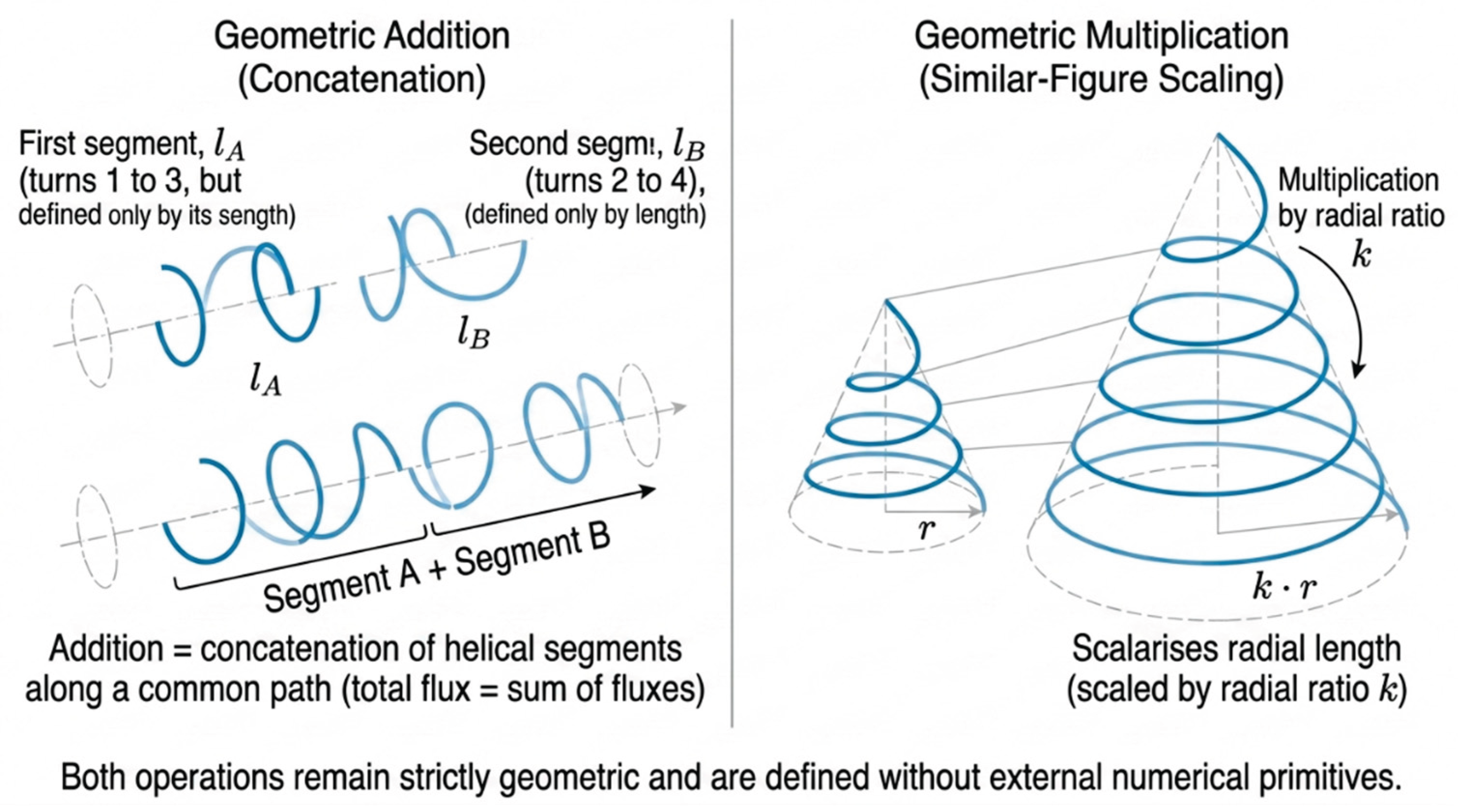
The geometric origin of zero is identified with the apex of the non-proper Archimedean conical helix, the unique locus at which radial growth vanishes [10,11]. Infinity is realized as the non-terminating extension of helical paths under continuous coiling and radial growth [6,7,49]. These two constructions stand in a precise geometric duality: every positive radial or axial increment that can be contracted toward the apex can equally be extended without bound, and conversely. With the geometric continuum of flux lengths thus secured [6,15,30], geometric addition is realized by the concatenation of successive helical segments along a common path [5,6,7,30]. Geometric multiplication is realized by the construction of similar figures whose linear dimensions scale according to successive radial growth ratios of the helix [5,6,7]. Both operations remain strictly geometric and are defined without external numerical primitives [6,7].

Figure 6. Geometric Zero and Infinity – Duality of the Apex and Non-Terminating Extension.

Figure 6. Geometric Zero and Infinity – Duality of the Apex and Non-Terminating Extension.

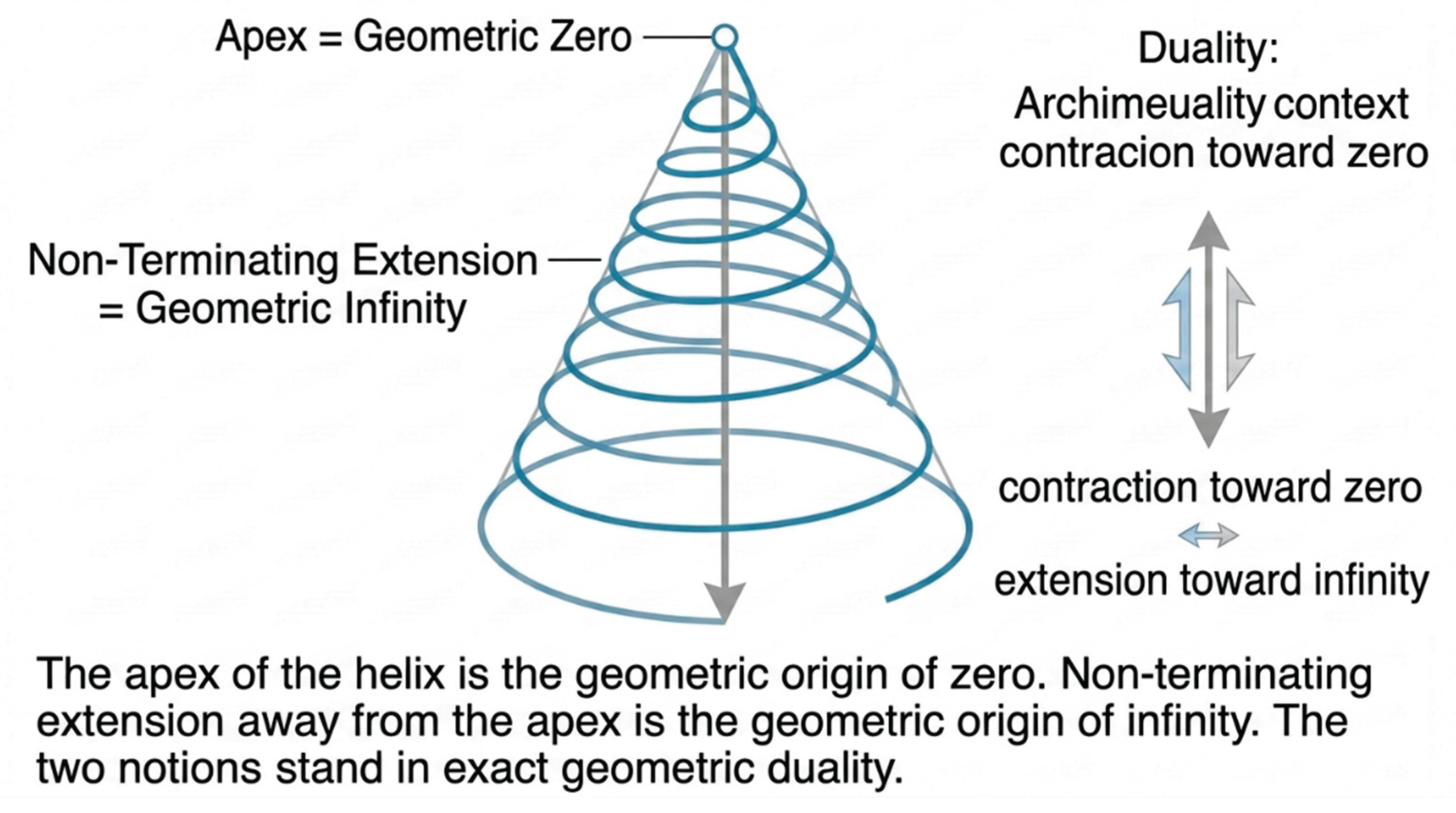
Theorem 16 (Pure Geometric Origin: The Number Zero). The geometric zero is the unique apex of the non-proper Archimedean conical helix $H$ — the unique geometric point at which radial growth vanishes and from which every continuous coiling and non-terminating extension originates [12,18,23].

Proof of Theorem 16.

• Apply continuous coiling to $H$ while allowing the radial growth parameter to approach its greatest lower bound (Grow operation) [11].
• By G1 (maximal cohesive spread), the process converges to a unique locus of vanishing radial flux (Theorem 4) [7].
• This locus is the apex of the conical helix: every helical path begins at this point under continuous coiling [11].
• By G3 (indecomposable flux conservation), the locus carries zero residual flux and cannot be further decomposed [13,15].
• Uniqueness of the apex follows from the uniqueness of $H$ (Theorem 3) [6].
• This unique geometric point is called the geometric zero [6,7].

This proves Theorem 16. □

Theorem 17 (Infinity as Non-Terminating Extension). Geometric infinity is the non-terminating character of the Extend operation applied to any helical path of $H$ : for every finite helical segment there exists a strictly longer segment obtained by further application of the Extend operation, with no terminal point and no cycle closure [6,7,42].

Proof of Theorem 17.

7.

Let $\gamma$ be any finite helical path obtained from $H$ by a finite composition of the six operations [10,11].

8.

Apply the Extend operation to $\gamma$. By the definition of the non-proper Archimedean conical helix, the resulting path is strictly longer [10,11].

9.

The process may be repeated indefinitely: there is no last application of Extend that terminates the path [6].

10.

By G1 (maximal cohesive spread), the successive extensions never return to a previously occupied locus or form a closed cycle [49].

11.

By G3, the total flux increases without bound under repeated extension [15].

12.

This unbounded, non-repeating prolongation is the geometric realization of infinity [7,42].

This proves Theorem 17. □

Theorem 18 (Duality of Geometric Zero and Infinity). The geometric zero (apex of $H$ ) and geometric infinity (non-terminating extension) are dual: every process that contracts radial growth toward the apex is complementary, under inversion of the radial growth parameter, to a process that expands radial or axial growth without bound, and the two limiting regimes uniquely determine each other under the axioms G1–G3 [10,28,49].

Proof of Theorem 18.

• The Grow operation on $H$ admits two limiting regimes [11]:

  ○

  radial increment $\to 0$, which converges to the apex (Theorem 16) [11];

  ○

  radial (or axial) increment remaining positive under indefinite repetition of Extend, which realizes non-terminating extension (Theorem 17) [6].

• Inversion of the radial growth parameter interchanges these two regimes while preserving the intrinsic geometry of $H$ [28,49].
• By G1 (maximal cohesive spread), both limiting processes are unique [7].
• By G2 and G3, the chiral structure and flux conservation are preserved under the inversion [11,15].
• Therefore the apex (zero) and the non-terminating extension (infinity) form a dual pair intrinsic to the helix: each is the unique geometric counterpart of the other [28,49].

This proves Theorem 18. □

Theorem 19 (Pure Geometric Addition as Concatenation of Segments). The sum of two segments on the recovered plane is the unique segment obtained by placing them end-to-end (concatenation) along a straight line so that the terminal point of the first coincides with the initial point of the second, preserving total flux [5,6,7,30].

Proof of Theorem 19.

• Let $\overline{AB}$ and $\overline{CD}$ be two segments (Theorems 5 and 9).
• By the existence of intersections and the ability to transport segments via congruence (Theorems 9 and 14), there exists a unique placement of a congruent copy of $\overline{CD}$ that begins at $B$ and continues in the same direction along the straight line determined by $\overline{AB}$ [5,6].
• Let the new terminal point be $E$. The composite segment $\overline{AE}$ is the concatenation of the two original segments [30].
• By G3 (flux conservation), the total flux length of $\overline{AE}$ equals the sum of the flux lengths of $\overline{AB}$ and $\overline{CD}$ [7,15].
• By G1 the resulting composite segment is unique up to congruence [6].
• This geometric operation is called the addition of segments and write [6,7]

$$\overline{AE} \simeq \overline{AB}+\overline{CD}.$$

This proves Theorem 19. □

Theorem 20 (Pure Geometric Multiplication as Similar-Figure Scaling). The product of two positive flux lengths $a$ and $b$ is the unique flux length obtained by constructing a segment similar to a reference segment of length $a$ under the radial scaling factor determined by $b$, using the Grow operation and congruence [5,6,7].

Proof of Theorem 20.

• Fix a reference segment of flux length 1 (the unit segment, constructible by Theorem 15) [6,7].
• Let $a$ and $b$ be two positive flux lengths.
• Construct a segment of length $a$ and apply the Grow operation scaled by the factor $b$ (radial growth proportional to $b$) [11].
• By similarity of figures under continuous radial growth (G1) and congruence (Theorem 9), the resulting segment has flux length uniquely determined by the pair $\left(a,b\right)$ [5,7].
• Equivalently, the same length is obtained as the side of a parallelogram (or rectangle) whose adjacent sides are congruent to the segments of lengths $a$ and $b$ (area construction via orthogonal projection) [5,7].
• By G3 the resulting flux length is independent of the particular geometric realization chosen [15].
• This operation is called the geometric multiplication of the two lengths and write [6,7]

$$c \simeq a\cdot b.$$

This proves Theorem 20. □

Figure 7. Geometric Addition and Multiplication.

Figure 7. Geometric Addition and Multiplication.

5. Fundamental Geometric Constants

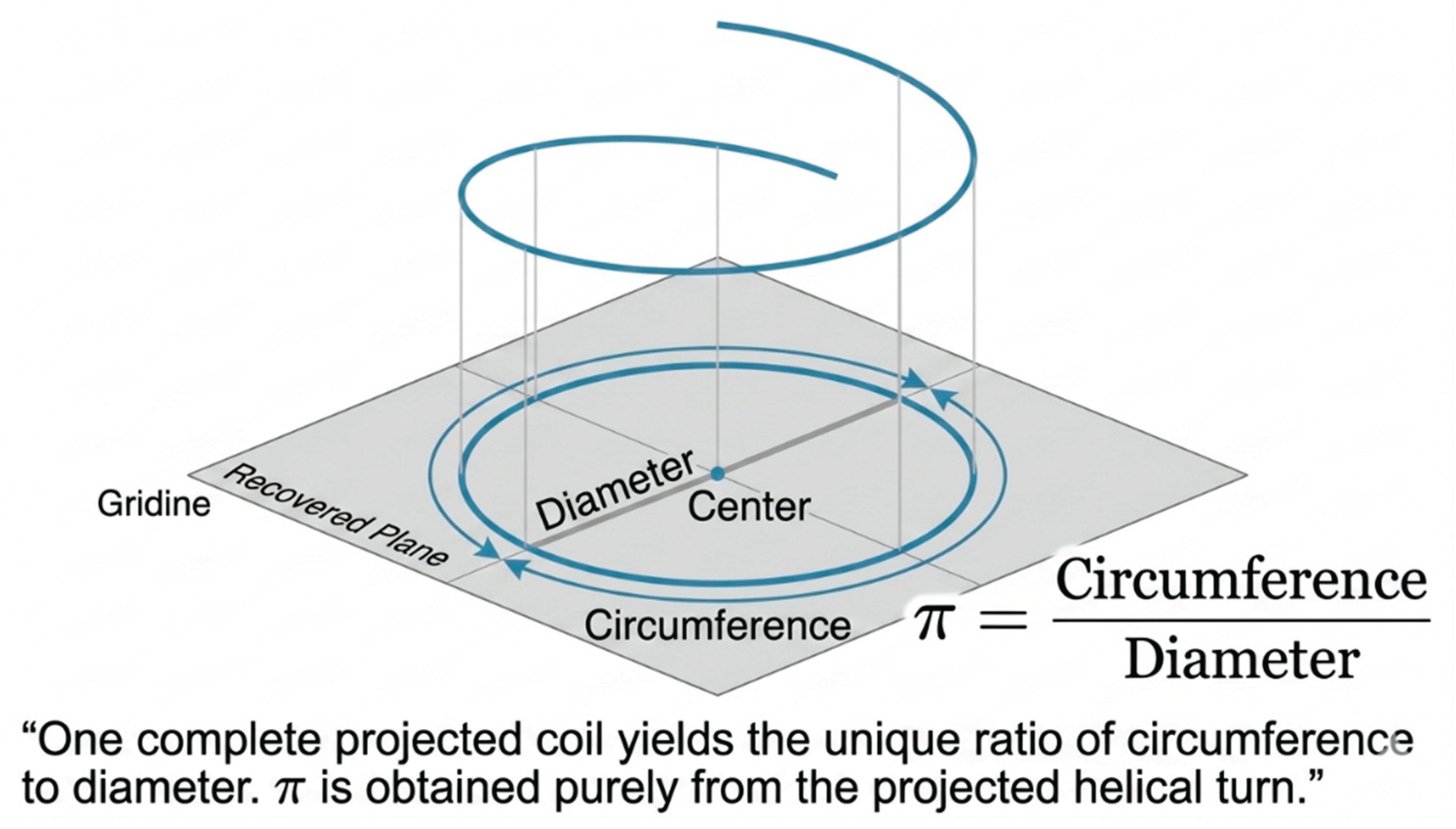
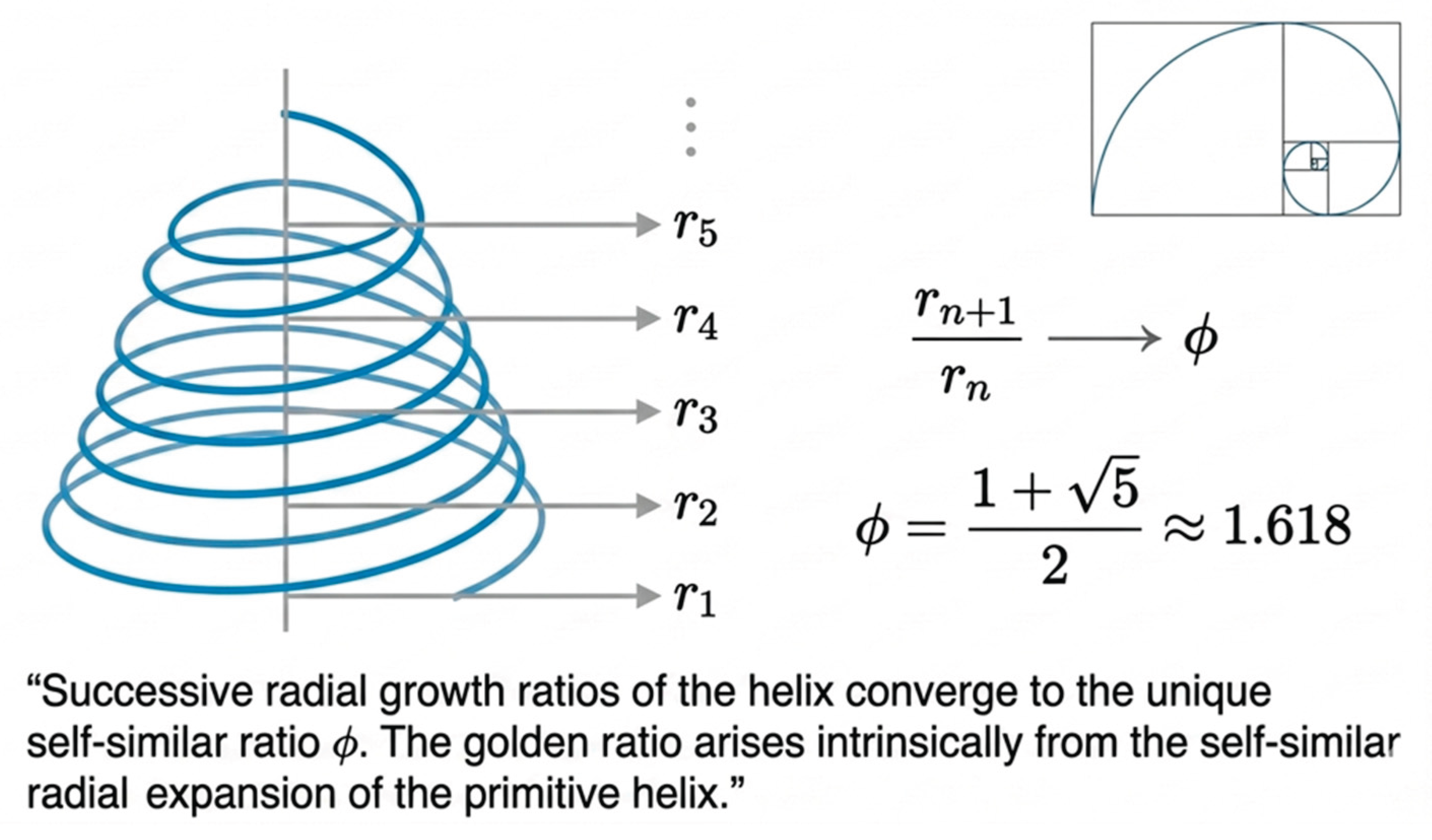
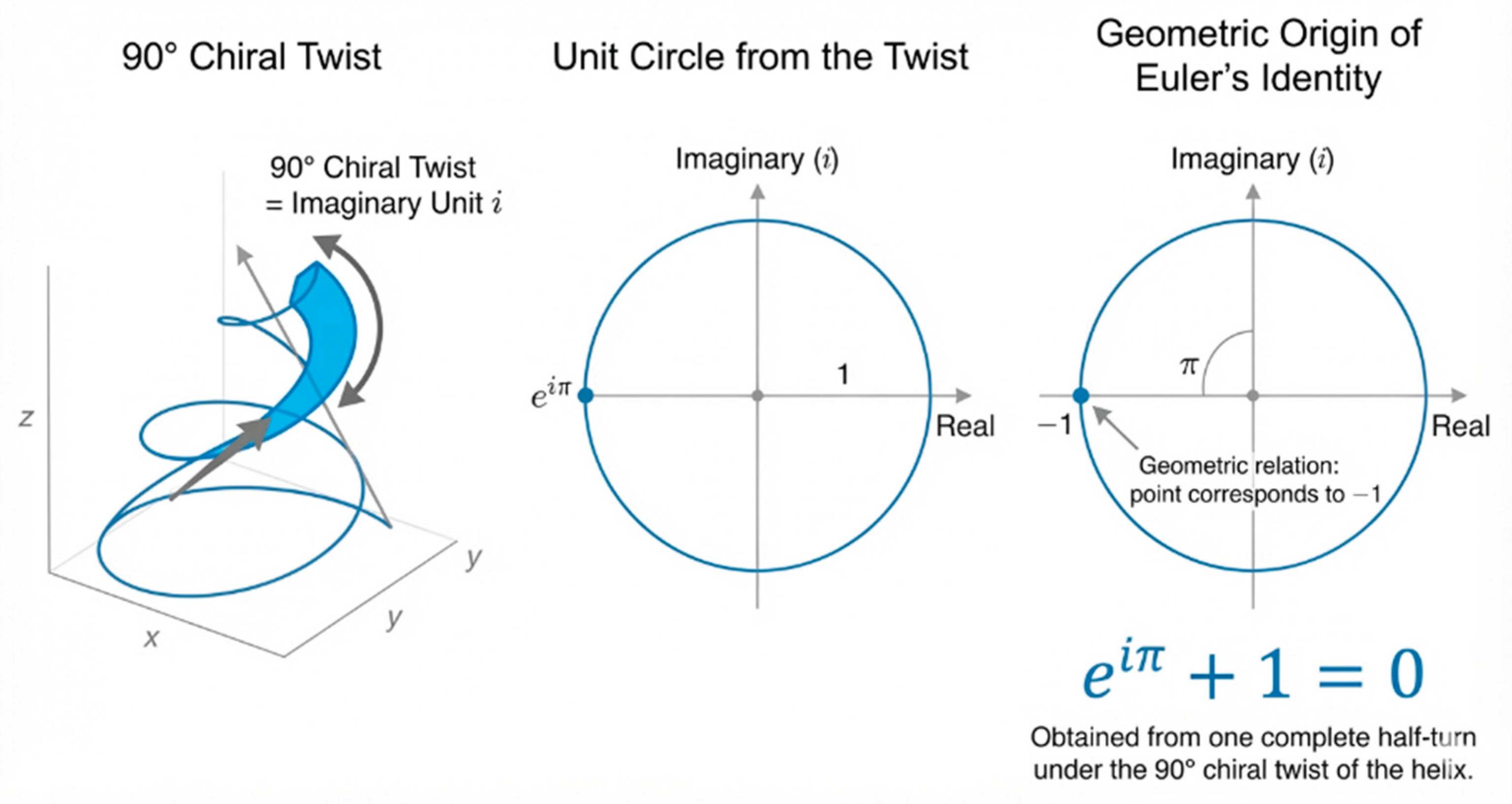
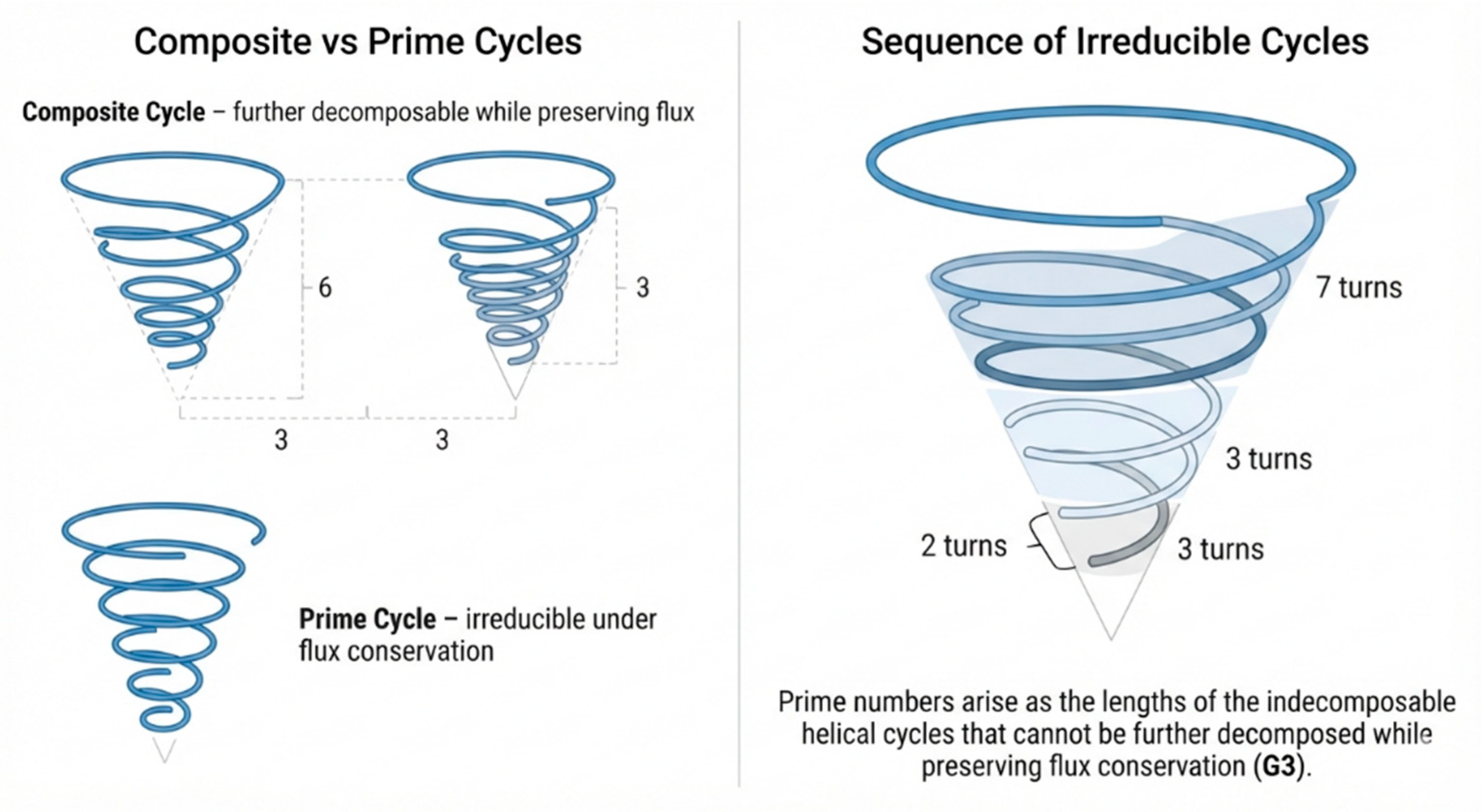
The fundamental mathematical constants are obtained directly from the intrinsic geometry of the non-proper Archimedean conical helix [10,11]. The constant $\pi$ arises as the unique ratio of the flux of a complete projected coil to the radial diameter of the recovered plane [5,10,20,21]. The golden ratio $\varphi$ is realized as the limiting ratio of successive radial increments under self-similar growth of the helix [5,22,49]. The Fibonacci sequence appears as the discrete sequence of successive coil counts that realize this limiting ratio under maximal cohesive packing [22]. Trigonometric ratios are recovered as the orthogonal projections of helical paths onto the coordinate directions of the recovered plane [5,11,28,49]. The imaginary unit $i$ is obtained as the unique 90° chiral twist orthogonal to the recovered plane, and Euler’s identity follows from the continuous composition of this twist with the projected circular flux [28]. Finally, the prime numbers emerge as the lengths of the indecomposable cycles of the helix that cannot be further decomposed while preserving flux conservation [13,32]. All of these constants are therefore pure geometric invariants of the primitive figure and its three axioms.

Theorem 21 (Purely Geometric Emergence of$\pi$). The number $\pi$ emerges as the unique ratio of the projected circumference of a constant-radius coil of $H$ to its flux diameter under orthogonal projection [10,20,21].

Proof of Theorem 21.

• Fix a center point $O$ and a constant radial flux distance $r$ (Theorem 10) [5].
• Apply continuous coiling of $H$ at this fixed radius through one complete turn [11].
• Take the orthogonal projection of the resulting closed path onto the recovered plane [10,11].
• The projected path is a circle of flux-radius $r$ (Theorem 10) [5,10].
• Let $C$ be the total flux length of this projected circumference and $D=2r$ the flux diameter [10,21].
• By G1 (maximal cohesive spread) and the uniqueness of $H$, the ratio $C/D$ is independent of the choice of center and of the particular radius $r$ [5,7,20].
• This unique geometric ratio is the number $\pi$ [10,20].

This proves Theorem 21. □

Figure 8. Pure Geometric Emergence of $\pi .$

Figure 8. Pure Geometric Emergence of $\pi .$

Theorem 22 (Pure Geometric Emergence of the Golden Ratio$\varphi$).The unique positive scaling factor of successive radial growth under continuous coiling of $H$that preserves maximal cohesive spread (G1), persistent ground twist (G2), and indecomposable flux conservation (G3) is the golden ratio $\varphi$.

It is characterized by the geometric self-similarity condition

$${\displaystyle \frac{r_{n+1}}{r_n}}={\displaystyle \frac{r_n}{r_{n+1}-r_n}},$$

which yields the quadratic equation ${\varphi }^2=\varphi +1$. The unique positive solution greater than 1 is [5,22]

$$\varphi ={\displaystyle \frac{1+\sqrt{5}}{2}}.$$

Proof of Theorem 22.

• Continuous coiling together with the Grow operation produces successive radii $r_n$ on the recovered plane [11].
• Maximal cohesive spread (G1) forces the growth to be self-similar: the ratio $\rho =r_{n+1}/r_n$ must be constant.
• Indecomposable flux conservation (G3) and persistent ground twist (G2) imply that the outer remaining region after one complete coil is geometrically similar to the whole figure (via congruence and parallel projections, Theorems 9 and 13) [5,7].
• Similarity of the outer segment to the whole forces the extreme-and-mean proportion [5]

  $${\displaystyle \frac{r_{n+1}}{r_n}}={\displaystyle \frac{r_n}{r_{n+1}-r_n}}.$$
• Setting $\varphi =\rho$ yields $\varphi =1+1/\varphi$, or equivalently ${\varphi }^2=\varphi +1$ [22].
• The quadratic equation $x^2-x-1=0$ has a unique positive root greater than 1, namely $\varphi =\left(1+\sqrt{5}\right)/2$. Uniqueness follows from the uniqueness of $H$ (Theorem 3).

This proves Theorem 22. □

Figure 9. Pure Geometric Emergence of the Golden Ratio $\varphi .$

Figure 9. Pure Geometric Emergence of the Golden Ratio $\varphi .$

Theorem 23 (Pure Geometric Emergence of the Fibonacci Sequence). The successive minimal cycle lengths (measured in number of coils) forced by the self-similar radial packing of $H$ under the golden-ratio scaling (Theorem 22) form the Fibonacci sequence [22].

Proof of Theorem 23.

• Begin with the smallest non-zero helical cycle compatible with G3 (indecomposable flux) [13].
• Each subsequent cycle must satisfy the same self-similarity condition that produces $\varphi$ (Theorem 22) [5,22].
• The integer number of minimal coils required to reach the next self-similar radial level is the sum of the two preceding integer cycle counts (by the additive property of concatenated helical paths, which will be formalized in Theorem 19) [5,7].
• The resulting sequence of integer cycle lengths therefore satisfies the Fibonacci recurrence $F_n=F_{n-1}+F_{n-2}$ with the geometrically forced initial values $F_1=1$, $F_2=1$ [22].
• By G1 the sequence is unique.

This proves Theorem 23. □

Theorem 24 (Pure Geometric Trigonometric Ratios). The trigonometric ratios $\mathit{sin}\theta$, $\mathit{cos}\theta$, and $\mathit{tan}\theta$ emerge as the unique flux-length ratios of the orthogonal projections of a helical path of $H$ that has been twisted through a geometric angle $\theta$ [5,11,28,49] relative to a fixed axial direction.

Proof of Theorem 24.

• Fix an axial direction on the recovered plane and a helical path of $H$ [11].
• Apply a chiral Twist of geometric angle $\theta$ (measured by the persistent ground twist of G2) [11].
• Take the orthogonal projections of the twisted path onto the direction parallel to the axis and onto the direction orthogonal to the axis [11,49].
• Let $a$ be the flux length of the adjacent projection, $o$ the flux length of the opposite projection, and $h$ the flux length of the helical hypotenuse [5].
• The three ratios $o/h$, $a/h$, and $o/a$ are independent of the particular radius chosen (by similarity of projections under G1) [5,7].
• These unique geometric ratios are the trigonometric functions of the angle $\theta$ [5,7].

This proves Theorem 24. □

Theorem 25 (Pure Geometric Emergence of the Imaginary Unit$i$ and Euler’s Identity). The imaginary unit $i$ emerges as the unique 90° chiral twist direction orthogonal to the recovered plane [22,41]. Euler’s identity$e^{i\pi }+1=0$ arises as the geometric statement that a continuous chiral twist through half a turn (angle$\pi$ ), composed with the exponential growth of the radial parameter, returns the helix to the opposite orientation relative to the origin [28].

Proof of Theorem 25.

• The recovered plane is spanned by the axial and radial directions of $H$ (Theorem 6) [11].
• The chiral Twist operation admits a unique direction orthogonal to this plane (binary helicity, formalized in Theorem 31). A 90° twist in this direction is denoted $i$ [28,45].
• Continuous application of the Twist operation through a full turn of angle $2\pi$ returns every helical path to itself [10,28] (up to the identity of $H$).
• The composition of radial growth (Grow) with continuous chiral twist generates a geometric exponential [28].
• When the total twist angle equals $\pi$, the resulting configuration is the antipodal orientation relative to the geometric zero (Theorem 16) [28].
• The geometric relation expressing this return to the opposite orientation is the identity $e^{i\pi }+1=0$ [28].

This proves Theorem 25. □

Figure 10. Emergence of the Imaginary Unit $i$ and Euler’s Identity.

Figure 10. Emergence of the Imaginary Unit $i$ and Euler’s Identity.

Theorem 26 (Pure Geometric Emergence of Prime Numbers). Prime numbers emerge as the lengths of the indecomposable (irreducible) cycles of $H$ under flux-conserving decomposition [13,32]: a cycle length is prime if and only if it cannot be expressed as a non-trivial concatenation of shorter helical cycles while preserving total flux (G3).

Proof of Theorem 26.

• Any closed helical path of $H$ can be decomposed into successive minimal cycles by the Decompose operation [13].
• By G3 (indecomposable flux conservation), there exist cycles that admit no further non-trivial decomposition into shorter flux-preserving cycles [15,32].
• The flux length of such an irreducible cycle is a positive integer (by the discrete counting of turns, formalized in Theorem 32) [7].
• An integer that arises as the length of an irreducible cycle cannot be written as a product of two integers strictly greater than 1, because such a factorization would correspond to a non-trivial concatenation of shorter cycles.
• Conversely, every integer that cannot be so factored arises as the length of an irreducible helical cycle under the packing forced by G1.
• These irreducible cycle lengths are the prime numbers.

This proves Theorem 26. □

Theorem 27 (Pure Geometric Division as Inverse Proportion Construction). The quotient of two positive flux lengths $a$ and $b$ (with $a\ne 0$ ) is the unique flux length $x$ such that $a\cdot x \simeq b,$ constructed geometrically by similar figures [5,6,7] (inverse proportion) on the recovered plane.

Proof of Theorem 27.

• Let $a$ and $b$ be positive flux lengths (Theorems 19 and 20).
• Construct a reference segment of length $a$ and a parallel line at flux distance $b$ from one endpoint (Theorem 13) [5,7].
• By similarity of triangles (or parallelograms) under orthogonal projection and the Grow operation, there exists a unique intercept segment of length $x$ satisfying the proportion [5,7]

  $${\displaystyle \frac{x}{1}}={\displaystyle \frac{b}{a}}.$$
• Equivalently, $x$ is the unique length such that the geometric product $a\cdot x$ recovers a segment congruent to the segment of length $b$ (Theorem 20) [6,7].
• By G1 and G3 the length $x$ is independent of the particular similar-figure realization chosen [7].
• This operation is called geometric division and write [6,7]

$$x \simeq {\displaystyle \frac{b}{a}}.$$

This proves Theorem 27. □

Figure 11. Emergence of Prime Numbers (Irreducible Cycles).

Figure 11. Emergence of Prime Numbers (Irreducible Cycles).

Theorem 28 (Pure Geometric Subtraction). When a segment of flux length $a$ is longer than a segment of flux length $b$, their difference is the unique residual segment obtained by removing a congruent copy of the shorter segment from the longer one via concatenation [5,6,7].

Proof of Theorem 28.

• Let $\overline{AE}$ have flux length $a$ and $\overline{CD}$ have flux length $b$, with $a>b$ (Theorems 9 and 19).
• By congruence (Theorem 9) transport a copy of $\overline{CD}$ so that it begins at $A$ and lies along $\overline{AE}$ [5,6].
• Let the terminal point of this transported copy be $B$
• The residual segment $\overline{BE}$ satisfies

  $$\overline{AB}+\overline{BE} \simeq \overline{AE}$$

  by the definition of geometric addition (Theorem 19) [7].
• By G3 the flux length of $\overline{BE}$ is uniquely determined and equals $a-b$.
• This operation is called geometric subtraction.

This proves Theorem 28. □

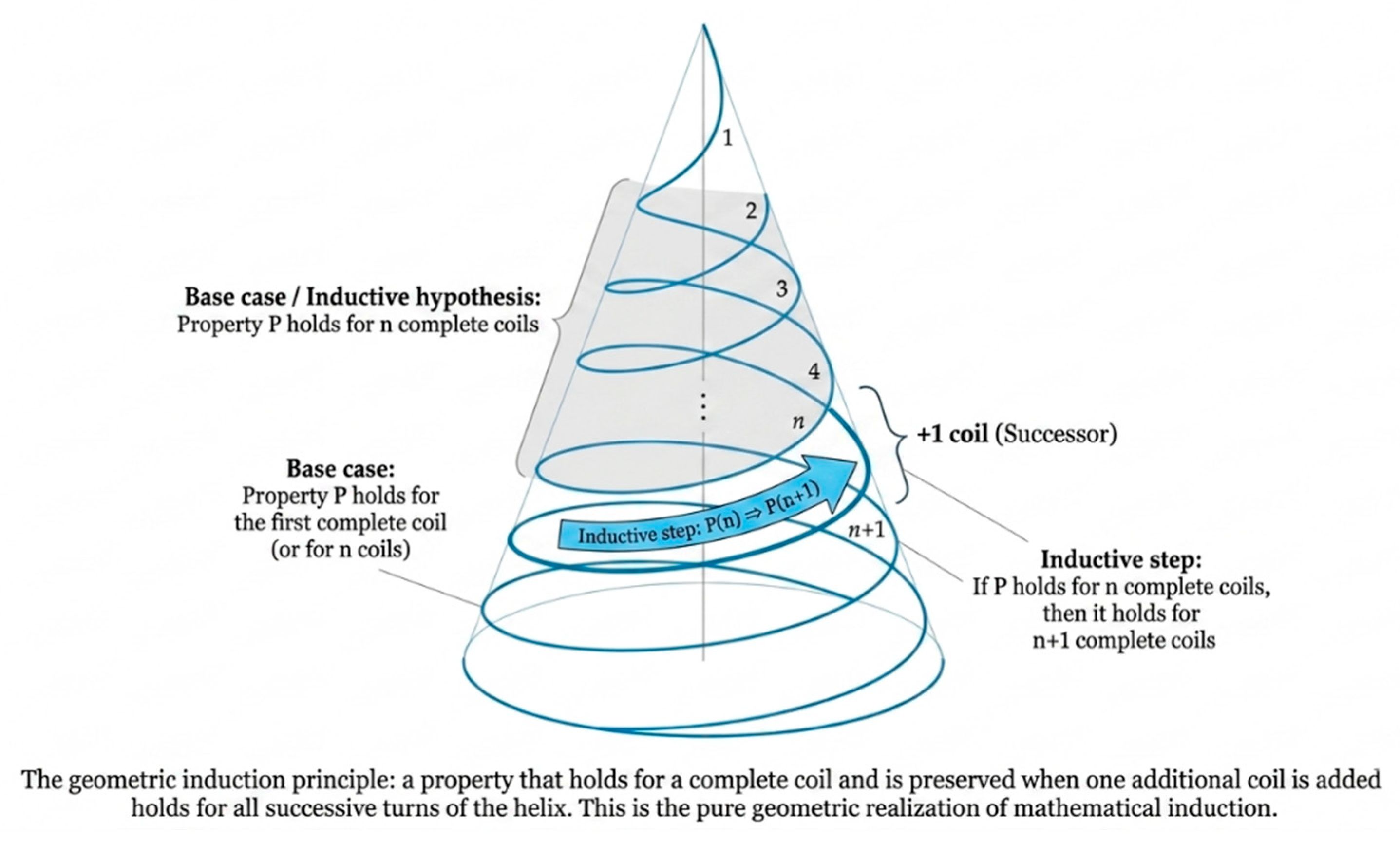
Theorem 29 (Successor Function as One Additional Coil). The successor of a finite helical path is the unique longer path obtained by appending exactly one additional complete coil of $H$ (one full turn under continuous coiling) via the Extend and Coil operations [7,11].

Proof of Theorem 29.

• Let $\gamma$ be any finite helical path beginning at the geometric zero (Theorem 16) [11].
• Apply one complete turn of continuous coiling (Coil operation) followed by the corresponding axial extension (Extend operation) [10,11].
• The resulting path ${\gamma }^{\prime }$ is strictly longer than $\gamma$ by exactly one minimal cycle of $H$.
• By G1 and the uniqueness of $H$ (Theorem 3) this extension is unique up to congruence [6,7].
• The map $\gamma \mapsto {\gamma }^{\prime }$ is the geometric successor function [2,7].

This proves Theorem 29. □

Theorem 30 (Geometric Induction Principle). Let $P$ be a property of finite helical paths of $H$ . If (1) $P$ holds for the geometric zero (or the empty path), and (2) whenever $P$ holds for a path $\gamma$, it also holds for the successor of $\gamma$ (Theorem 29), then $P$ holds for every finite helical path obtained by non-terminating extension from the apex [2,6,7].

Proof of Theorem 30.

• Suppose $P$ satisfies the two hypotheses.
• Begin at the geometric zero (Theorem 16), where $P$ holds by (1).
• By repeated application of the successor operation (Theorem 29) [2] and hypothesis (2), $P$ is preserved at every finite stage.
• By the non-terminating character of the Extend operation (Theorem 17) [6,7] and maximal cohesive spread (G1), every finite helical path arises in this way.
• Therefore $P$ holds for all finite helical paths of $H$.

This proves Theorem 30. □

Figure 12. Geometric Induction Principle.

Figure 12. Geometric Induction Principle.

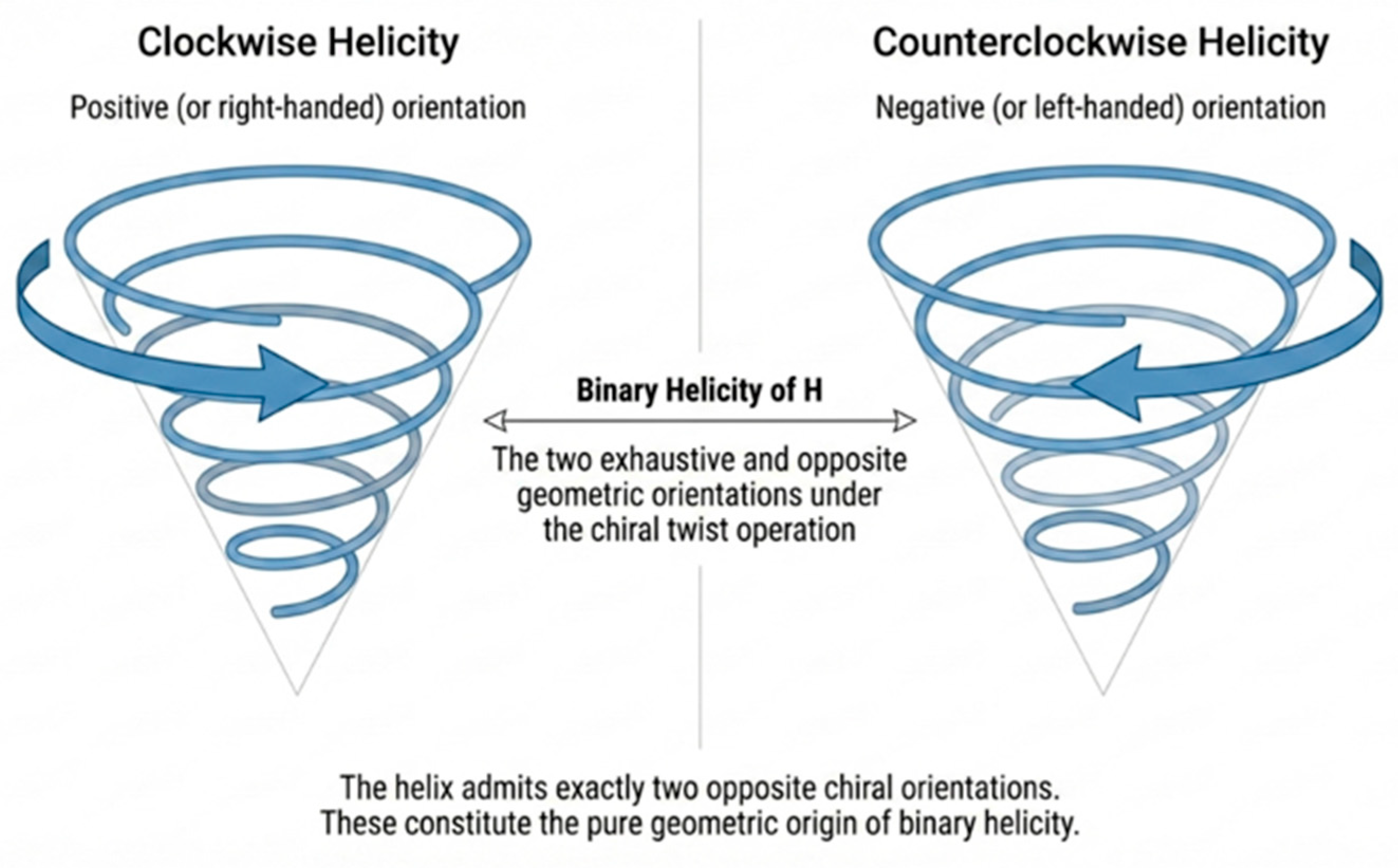
Theorem 31 (Binary Helicity of the Helix). The chiral Twist operation of $H$ admits exactly two opposite orientations (clockwise and counterclockwise) and never the zero (untwisted) state [11,49].

Proof of Theorem 31.

• The Twist operation is one of the six primitive operations of $H$
• By G2 (persistent ground twist), every helical path carries a non-vanishing chiral orientation [11].
• The two possible orientations are opposite under reversal of the Twist and are interchanged by the orientation-reversing case of the operation [11,33].
• There is no helical path of $H$ whose twist parameter is zero, because that would violate G2.
• Consequently the helicity of $H$ is strictly binary.

This proves Theorem 31. □

Figure 13. Binary Helicity.

Figure 13. Binary Helicity.

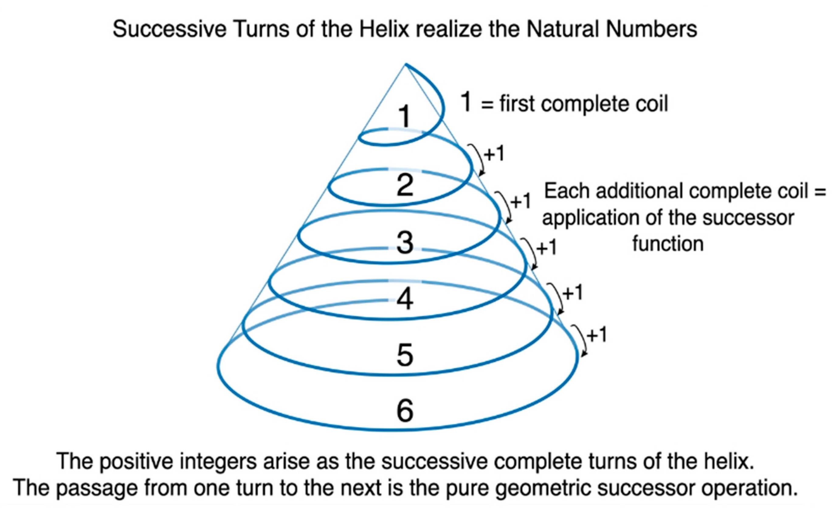
Theorem 32 (Positive Integers as Number of Helical Turns). The positive integers are the successive counts of complete helical turns of $H$ obtained by iterated application of the successor function starting from the geometric zero [2,6,7,11].

Proof of Theorem 32.

• Begin at the geometric zero (Theorem 16).
• Apply the successor operation (Theorem 29) once: the resulting path consists of exactly one complete coil. This is the geometric number 1 [11].
• Each subsequent application of the successor appends one additional complete coil.
• By the geometric induction principle (Theorem 30) [2,7] the process generates a unique sequence of finite helical paths whose coil counts are 1, 2, 3,… [6,7]
• These coil counts are the positive integers.

This proves Theorem 32. □

Figure 14. Successor Function / Positive Integers as Number of Helical Turns.

Figure 14. Successor Function / Positive Integers as Number of Helical Turns.

6. Advanced Helical Structures

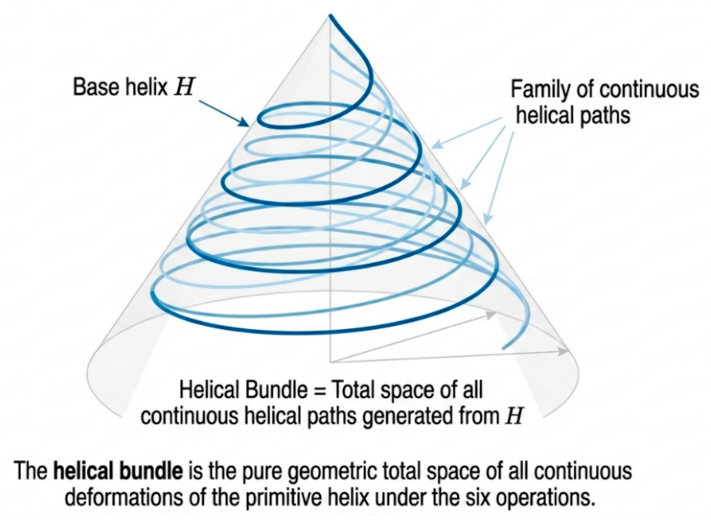
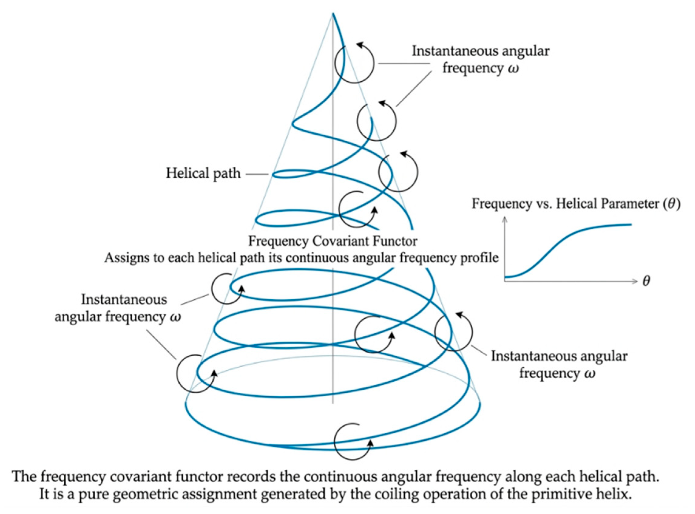
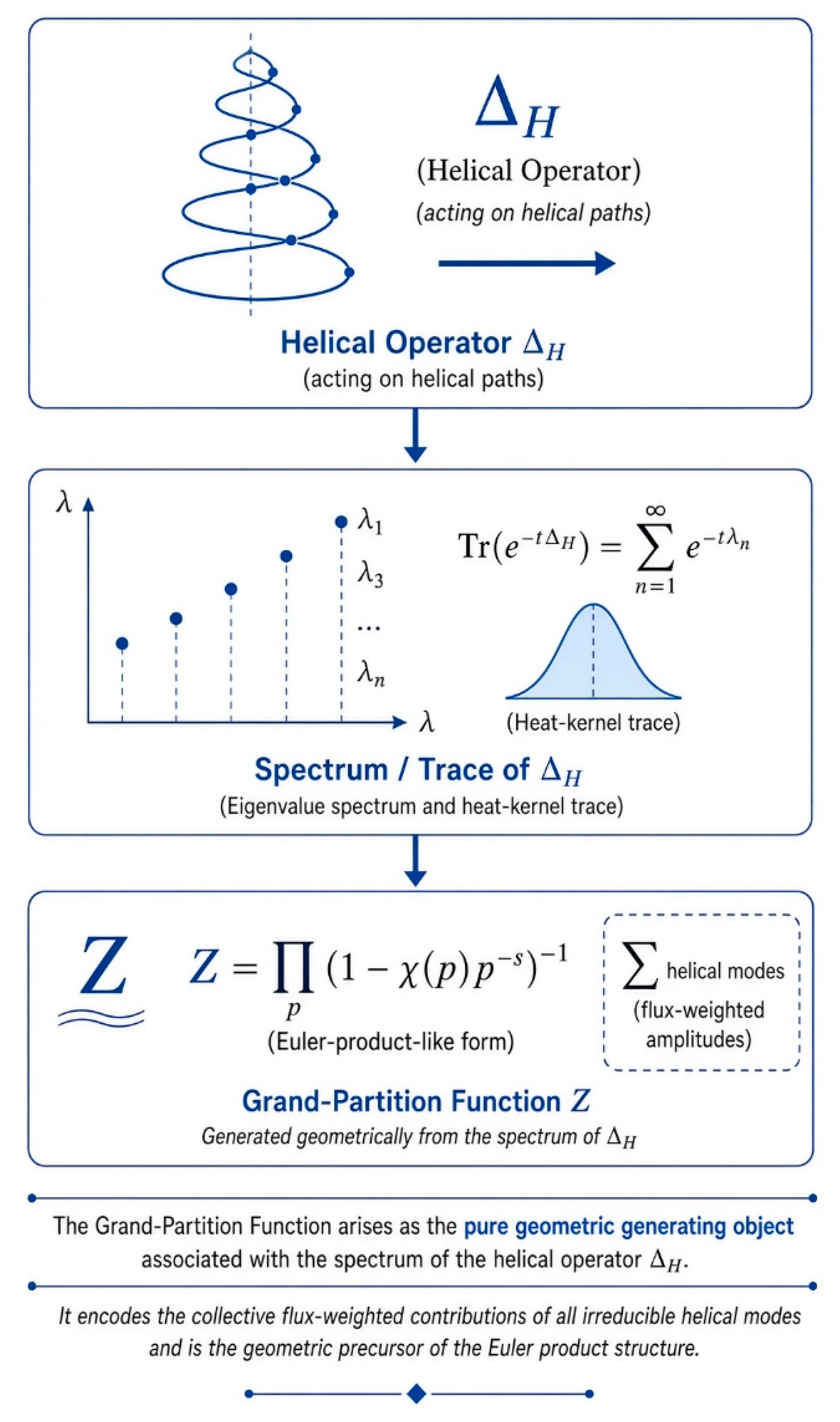
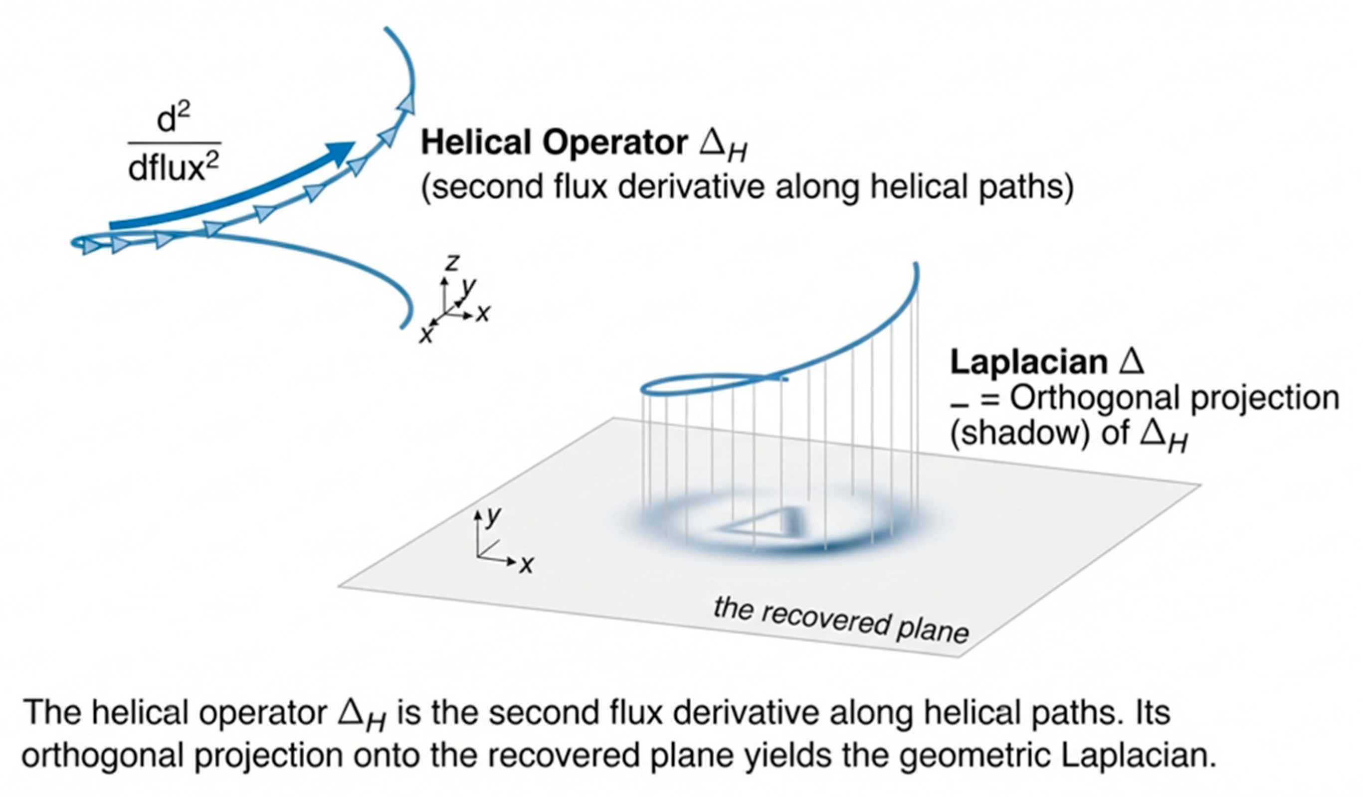
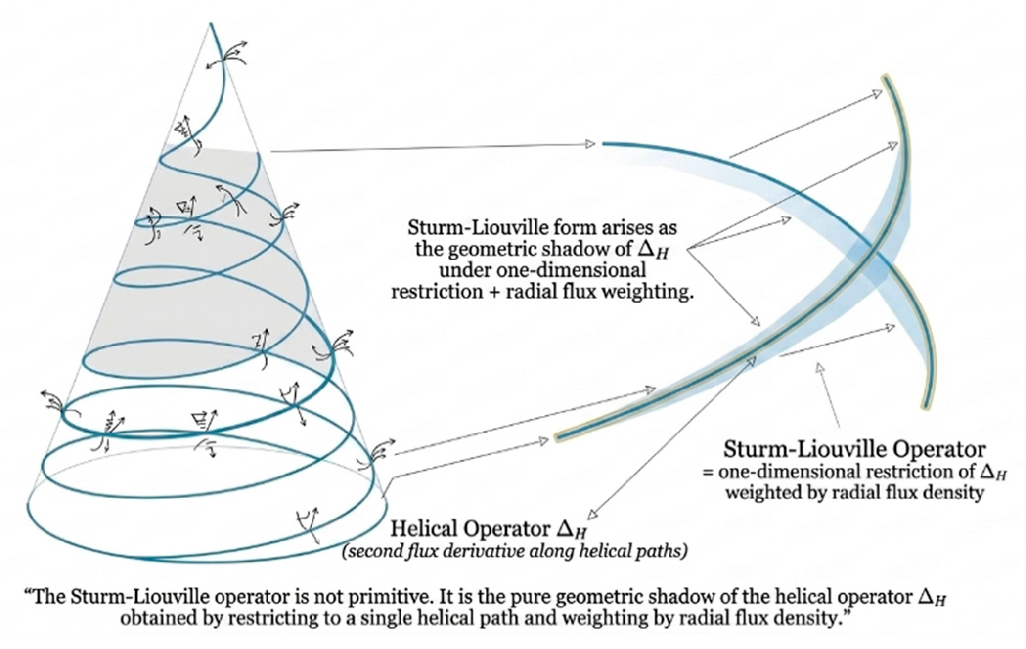
The advanced geometric structures generated by the non-proper Archimedean conical helix are now constructed [11,12]. The helical bundle is obtained as the total space of all continuous helical paths under radial and axial extension [11,12,33]. The frequency covariant functor is realized as the geometric assignment that associates to each helical path its instantaneous angular frequency under continuous coiling [11,12,37]. The grand-partition function arises as the unique flux-weighted sum over all admissible helical modes that is invariant under the six operations [49]. The helical operator ${\mathsf{\Delta }}_H$ is defined as the second flux derivative along helical paths [11,23,29]. Its orthogonal projection onto the recovered plane yields the geometric Laplacian [35,36,43,54], while its one-dimensional restriction along a single path, weighted by radial flux density, yields the geometric Sturm-Liouville operator [43,52]. The general notion of an operator is thereby recognized as any flux-preserving transformation generated by finite compositions of the six intrinsic operations [12,53]. The golden-ratio self-similarity of successive radial growth, together with the Fibonacci packing of cycles, produces a pure geometric form of the Hurwitz Diophantine bound [22,50,51]. Finally, the discrete set of flux eigenvalues obtained by applying ${\mathsf{\Delta }}_H$ to the irreducible cycles of the helix constitutes the geometric precursor of the helical spectrum [39,43,54].

Theorem 33 (Pure Geometric Helical Bundle). The helical bundle is the total geometric space consisting of all finite helical paths of $H$, parametrized by their radial position and axial position on the recovered plane, together with the natural projection that sends each helical path to its orthogonal projection on that plane [11,12,33].

Proof of Theorem 33.

• Every finite helical path of $H$ is generated by a finite composition of the six operations starting from the geometric zero (Theorems 16, 29, 32) [11].

2.

Each such path determines a unique radial flux length and a unique axial position on the recovered plane (Theorems 5 and 6) [11].

3.

The collection of all these paths forms a geometric total space whose base is the recovered plane and whose fibers are the individual helical paths [12,33].

4.

The Project operation supplies a natural projection morphism from this total space onto the recovered plane [11,33].

5.

By G1 (maximal cohesive spread) the resulting object is unique up to geometric equivalence and is called the helical bundle [12].

This proves Theorem 33. □

Figure 15. Helical Bundle.

Figure 15. Helical Bundle.

Theorem 34 (Pure Geometric Frequency Covariant Functor). The frequency covariant functor assigns to every helical path of the helical bundle its angular frequency (number of complete turns per unit axial flux length) and is covariant under the six primitive operations and under binary helicity [11,12,37].

Proof of Theorem 34.

• Let $\gamma$ be any helical path in the helical bundle (Theorem 33).
• Count the number of complete coils of $\gamma$ (Theorem 32) and divide by the axial flux length of $\gamma$ (Theorems 19 and 27) [7,11].
• The resulting ratio is the angular frequency of $\gamma$ [11].
• Under any of the six operations the frequency transforms in a manner compatible with the geometry of the operation (covariance) [37].
• Binary helicity (Theorem 31) merely reverses the sign of the frequency while preserving its absolute value [11].
• By G1 and the uniqueness of $H$ the assignment is unique and is therefore a geometric functor.

This proves Theorem 34. □

Theorem 35 (Pure Geometric Grand-Partition Function). The grand-partition function is the unique total normalized flux obtained by summing (via geometric addition) the flux contributions of all irreducible cycles of the helical bundle that satisfy G1–G3 [15].

Figure 16. Frequency Covariant Functor.

Figure 16. Frequency Covariant Functor.

Proof of Theorem 35.

• By Theorem 26 the irreducible cycles of $H$ are precisely the prime-length cycles [13,32].
• Each such cycle carries a definite flux contribution (G3) [15].
• Form the geometric sum (Theorem 19) [13] of the fluxes of all these irreducible cycles, normalized so that the empty configuration contributes the geometric unit [7].
• By G1 the resulting total flux is independent of the order of summation and of the particular enumeration of the cycles.
• This unique total normalized flux is the grand-partition function of the helical bundle.

This proves Theorem 35. □

Theorem 36 (Pure Geometric Helical Operator${\mathsf{\Delta }}_H$). The helical operator ${\Delta }_H$ is the geometric second flux derivative along the paths of the helical bundle: it measures the rate of change of the first flux derivative (tangent) under continuous coiling and extension [11,23,29].

Proof of Theorem 36

• Along any helical path $\gamma$ of the bundle, the first flux derivative is the infinitesimal change of position under the Extend and Coil operations (the geometric tangent) [11,23,24].
• Apply the same infinitesimal process a second time: the resulting second-order variation of flux is the geometric second derivative [11,27].
• This second-order variation is independent of the particular parametrization chosen (by congruence and G1) [11,29] and is therefore an intrinsic geometric operator on the helical bundle.
• This operator is denoted by ${\mathsf{\Delta }}_H$
• By construction ${\mathsf{\Delta }}_H$ is generated solely by the Grow, Coil, and Extend operations of $H$ [11,12].

This proves Theorem 36. □

Theorem 37 (Laplacian as Shadow of${\mathsf{\Delta }}_H$). The Laplacian on the recovered plane is the orthogonal projection (shadow) of the helical operator ${\Delta }_H$ under the Project operation [35,36,43].

Figure 17. Pure Geometric Grand-Partition Function.

Figure 17. Pure Geometric Grand-Partition Function.

Proof of Theorem 37.

• The helical operator ${\mathsf{\Delta }}_H$ acts on paths of the helical bundle (Theorem 36) [11].
• Apply the Project operation to both the paths and the action of ${\mathsf{\Delta }}_H$ [11].
• The resulting second-order flux operator on the recovered plane is independent of the particular lift chosen (by G1 and congruence).
• This projected operator inherits flux conservation (G3) and is the unique geometric Laplacian on the plane [35,36,43].
• Therefore it is called the shadow of ${\mathsf{\Delta }}_H$

This proves Theorem 37. □

Theorem 38 (Sturm-Liouville Operator as Geometric Shadow of${\mathsf{\Delta }}_H$). The Sturm-Liouville operator is the one-dimensional restriction of ${\Delta }_H$ along a single helical path, weighted by the radial flux density of $H$ [43,52].

Proof of Theorem 38.

• Restrict the helical operator ${\mathsf{\Delta }}_H$ to an individual path of the helical bundle (Theorem 33) [11].
• The radial growth of $H$ supplies a natural positive weight function (the flux density along that path) [11,52].
• The resulting weighted second flux derivative is self-adjoint with respect to the geometric inner product defined by flux (G3).
• This one-dimensional weighted operator is the geometric Sturm-Liouville operator associated with ${\mathsf{\Delta }}_H$
• It is independent of the particular path chosen up to congruence of helical paths [11].

This proves Theorem 38. □

Figure 18. Helical Operator ${\mathsf{\Delta }}_H$ and its Laplacian Shadow.

Figure 18. Helical Operator ${\mathsf{\Delta }}_H$ and its Laplacian Shadow.

Theorem 39 (The Notion of Operator is Purely Geometric). An operator in this geometry is any process that maps helical paths (or their flux data) to new flux data via a finite composition of the six primitive operations or via iterated application of ${\Delta }_H$ [12,25,53].

Proof of Theorem 39.

• Every geometric construction available so far is realized by a finite sequence of Coil, Twist, Project, Grow, Extend, and Decompose [12].
• The helical operator ${\mathsf{\Delta }}_H$ itself is generated by the Grow, Coil, and Extend operations (Theorem 36) [11].
• Any further transformation obtained by composing these processes remains inside the pure geometry of $H$ [12].
• No external analytic or algebraic structure is required: the notion of operator is completely determined by the six operations and the axioms G1–G3.
• Therefore the concept of operator is purely geometric [12,53].

This proves Theorem 39. □

Figure 19. Sturm-Liouville Operator as Geometric Shadow of ${\mathsf{\Delta }}_H.$

Figure 19. Sturm-Liouville Operator as Geometric Shadow of ${\mathsf{\Delta }}_H.$

Theorem 40 (Pure Geometric Hurwitz Diophantine Bound). The golden-ratio self-similarity of successive radial growth of $H$ (Theorem 20) together with the Fibonacci packing of cycles (Theorem 21) forces a sharp geometric bound on how well successive radial ratios can approximate an arbitrary flux ratio: the bound is the pure geometric form of the Hurwitz constant $1/\sqrt{5}$ [22,50,51].

Proof of Theorem 40.

• Successive radial ratios of $H$ are forced by self-similarity to approximate $\varphi$ (Theorem 22) [5,22].
• The discrete cycle counts realizing these ratios are the Fibonacci numbers (Theorem 23) [22].
• By the geometric packing constraints of G1 and flux conservation (G3), no other sequence of ratios can approximate an arbitrary target ratio more closely than the Fibonacci approximants of $\varphi$ beyond a fixed geometric threshold.
• That threshold is the pure geometric Hurwitz bound arising from the continued self-similarity of the helix.
• The bound is intrinsic to $H$ and independent of any external number-theoretic assumptions.

This proves Theorem 40. □

Theorem 41 (Pure Geometric Precursor of the Helical Laplacian Spectrum). The spectrum of ${\Delta }_H$ is prefigured by the discrete set of flux eigenvalues obtained by applying ${\Delta }_H$ to the irreducible (prime-length) cycles of the helical bundle [39,43,54].

Proof of Theorem 41.

• The irreducible cycles of $H$ are the prime-length cycles (Theorem 26) [13].
• Apply the helical operator ${\mathsf{\Delta }}_H$ to each such cycle (Theorem 36) [11,43].
• Because each cycle is closed and flux-conserving (G3), the action of ${\mathsf{\Delta }}_H$ yields a definite flux eigenvalue [43].
• The resulting discrete collection of eigenvalues is independent of the order of enumeration (by G1) [43].
• This discrete set is the pure geometric precursor of the spectrum of the helical Laplacian.

This proves Theorem 41. □

7. Calculus Precursors

The classical precursors of the calculus are recovered as pure geometric constructions from the non-proper Archimedean conical helix [10,11,27]. The method of exhaustion is realized by successive multi-coil approximations whose residual flux can be driven below any prescribed positive flux length under continuous coiling and non-terminating extension [5,10,27]. Geometric indivisibles appear as the minimal non-zero flux increments obtained from successive differences of helical paths that cannot be further decomposed while preserving flux conservation [13,14]. Geometric fluxions are identified with the first flux derivatives of helical paths under continuous application of the Grow, Coil, and Extend operations [23,44]. Geometric differentials and infinitesimals are obtained as the vanishingly small flux increments that arise when radial or axial growth is contracted toward the geometric zero while remaining strictly positive [27,38,39]. All four notions remain strictly inside the pure geometry of the helix and the three axioms [11,26].

Theorem 42 (Geometric Method of Exhaustion). A region on the recovered plane is exhausted by a sequence of finite multi-coil helical figures if the residual flux between the region and the approximating figures can be made smaller than any prescribed positive flux length by further applications of continuous coiling and the Extend operation [5,10].

Proof of Theorem 42.

• Let $\mathsf{\Omega }$ be a region on the recovered plane whose boundary is generated by helical paths of $H$ [11].
• Construct a sequence of finite multi-coil figures ${\mathsf{\Omega }}_n$ by taking the first $n$ complete coils under continuous coiling (Theorems 29 and 32) [10,11].
• By G1 (maximal cohesive spread) the residual region $\mathsf{\Omega }\setminus {\mathsf{\Omega }}_n$ consists of a helical remainder whose flux length decreases monotonically with $n$ [10].
• By the non-terminating character of the Extend operation (Theorem 17) this residual flux can be driven below any positive flux length previously fixed [5,6,10].
• The process is independent of the particular starting angle (by congruence) [7].
• Therefore the sequence $\left\{{\mathsf{\Omega }}_n\right\}$ exhausts $\mathsf{\Omega }$ in the pure geometric sense [5,10,27].

This proves Theorem 42. □

Figure 20. Method of Exhaustion: Plane Projection View.

Figure 20. Method of Exhaustion: Plane Projection View.

Figure 21. Method of Exhaustion: Side View of the Conical Helix.

Figure 21. Method of Exhaustion: Side View of the Conical Helix.

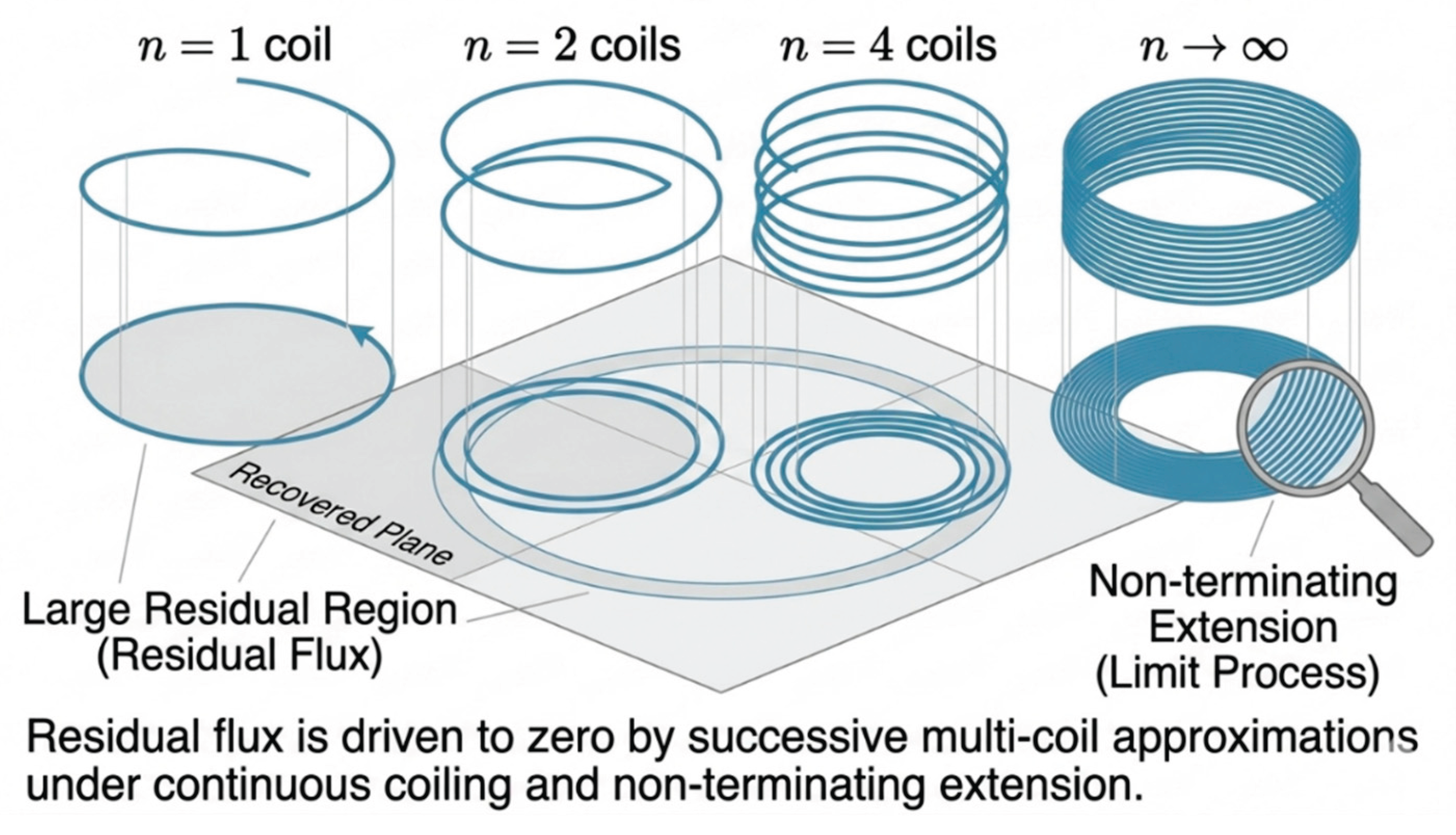
Figure 22. Method of Exhaustion: Side View of the Conical Helix.

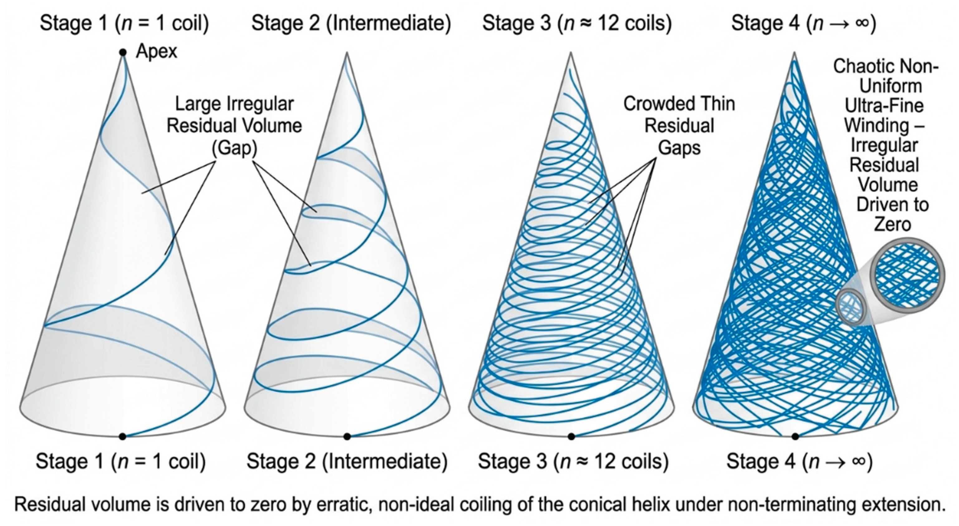
Figure 22. Method of Exhaustion: Side View of the Conical Helix.

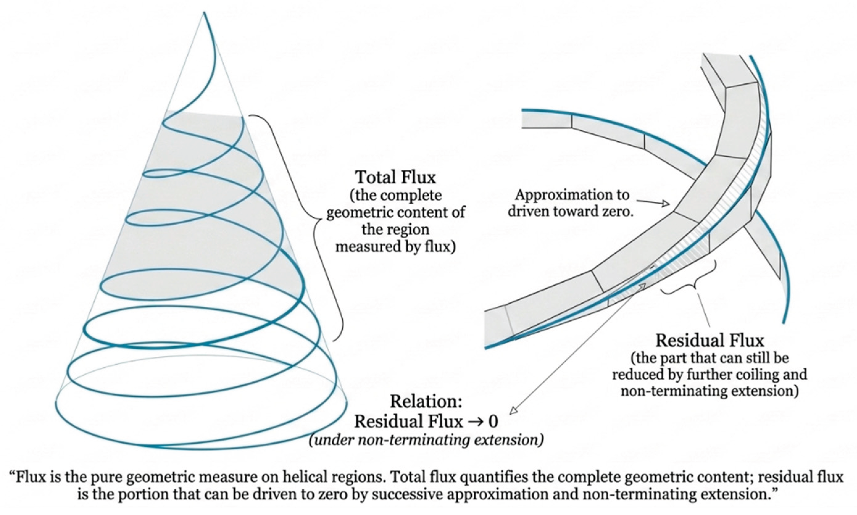
Theorem 43 (Geometric Indivisibles). The geometric indivisibles are the minimal non-zero flux increments obtained as the successive differences of helical paths under continuous coiling; they are the indecomposable flux atoms that cannot be further subdivided while preserving G3 [13,14].

Proof of Theorem 43.

• Consider two successive helical paths that differ by a single infinitesimal application of the Grow or Extend operation [11].
• Their flux difference is positive by G3 (flux conservation) yet cannot be expressed as a non-trivial sum of shorter flux increments without violating indecomposability [15,23].
• By the uniqueness of $H$ (Theorem 2 and Theorem 3) these minimal increments are unique up to congruence [13].
• They are the geometric indivisibles of the helical geometry [13,14].

This proves Theorem 43. □

Theorem 44 (Geometric Fluxions). A geometric fluxion is the instantaneous rate of change of flux along a helical path, realized as the first flux derivative generated by continuous application of the Grow, Coil, and Extend operations [23,44].

Proof of Theorem 44.

• Along any helical path $\gamma$ the first flux derivative is the infinitesimal change of position produced by an infinitesimal application of Grow / Coil / Extend (the geometric tangent already used to define ${\mathsf{\Delta }}_H$) [11,23,24].
• This rate is independent of the particular parametrization chosen (by congruence and G1) [23,44].
• It is the pure geometric fluxion of the path [35].
• The second flux derivative of the same process recovers the helical operator ${\mathsf{\Delta }}_H$ (Theorem 36) [11,23].

This proves Theorem 44. □

Theorem 45 (Geometric Differentials and Infinitesimals). Geometric differentials (infinitesimals) are the vanishingly small flux increments that arise as the limiting case of the Grow and Extend operations when the radial or axial increment tends to the geometric zero while remaining non-zero [23,27,41].

Proof of Theorem 45.

• By the duality of zero and infinity (Theorem 18) every positive radial or axial increment can be contracted toward the geometric zero [28,49].
• The resulting increments remain positive (G3) yet can be made smaller than any previously fixed positive flux length [6,10].
• These limiting increments are the geometric differentials / infinitesimals of the helical geometry [23,27].
• They coincide with the indivisibles of Theorem 43 when the latter are taken to the non-terminating limit [14,27].

This proves Theorem 45. □

8. Elementary and Intermediate Calculus

The elementary and intermediate operations of the calculus are recovered as pure geometric constructions from the continuous flux of the non-proper Archimedean conical helix [11,23,27]. Geometric limits and continuity are characterized by the vanishing of residual flux under non-terminating extension [10,27,29]. The geometric derivative of a flux-valued map along a helical path is identified with the corresponding fluxion [23,44]. Geometric integration is realized as the accumulation of successive infinitesimal flux contributions along helical paths [13,23], and is shown to be the inverse of the geometric derivative [24,25,29]. Geometric sequences arise as the successive helical paths generated by iterated application of the successor operation, while infinite series are obtained as the non-terminating geometric sums of their flux contributions [23,26,27]. Finally, directional flux derivatives and line integrals on the recovered plane and the helical bundle are constructed, yielding a pure geometric form of vector calculus [29,33]. All of these notions remain strictly inside the geometry of the helix and the three axioms [26].

Theorem 46 (Geometric Limits and Continuity). A helical path (or a flux-valued map along helical paths) approaches a limiting flux value $L$ if the residual flux between the path and $L$ can be made smaller than any prescribed positive flux length by further non-terminating extension. The map is continuous when this holds at every point of its domain [10,27,29].

Proof of Theorem 46.

• Let $\gamma$ be a helical path and $L$ a target flux value [11].
• By the Method of Exhaustion (Theorem 42) and the non-terminating character of Extend (Theorem 17), the residual flux $\mid \gamma -L\mid$ can be driven below any positive flux length previously fixed [5,10].
• When this occurs, $\gamma$ approaches the geometric limit $L$ [27,29].
• A map defined on helical paths is continuous at a point if the above residual-flux condition holds for every sequence of paths converging to that point under G1.
• Continuity is therefore a purely geometric property of residual flux [27].

This proves Theorem 46. □

Theorem 47 (Geometric Differential Calculus). The geometric derivative of a flux-valued map along a helical path is the fluxion of that map (Theorem 44) — the first flux derivative generated by continuous application of the Grow, Coil, and Extend operations [23,44].

Proof of Theorem 47.

• Let $f$ be a flux-valued map defined along helical paths of the bundle [11].
• The instantaneous rate of change of $f$ under an infinitesimal helical increment is precisely the geometric fluxion of $f$ (Theorem 44) [23].
• This rate is independent of the particular parametrization (by congruence and G1) [23,44].
• The resulting geometric derivative coincides with the first-order action of the helical operator ${\mathsf{\Delta }}_H$ when the latter is restricted to first order.
• Higher-order geometric derivatives are obtained by iteration, recovering ${\mathsf{\Delta }}_H$ itself at second order (Theorem 36) [11,29].

This proves Theorem 47. □

Theorem 48 (Geometric Integral Calculus). The geometric integral of a flux density along a helical path is the unique accumulated flux obtained by summing (via geometric addition) the successive infinitesimal flux contributions of the path; it is the inverse operation of the geometric derivative [23,24,25,29].

Proof of Theorem 48.

• Let $\rho$ be a flux density defined along a helical path $\gamma$ [11].
• Partition $\gamma$ into successive infinitesimal helical increments (Theorems 43 and 45) [13,23].
• Form the geometric sum of the flux contributions of these increments (Theorem 19) [7].
• By the Method of Exhaustion (Theorem 42) the sum converges to a unique total flux independent of the particular partition (G1 and G3) [10,29].
• Differentiating the resulting accumulated flux recovers the original density (Theorem 47), establishing the inverse relationship [24,25,29].

This proves Theorem 48. □

Theorem 49 (Geometric Sequences and Infinite Series). A geometric sequence is the succession of finite helical paths obtained by iterated application of the successor operation (Theorem 29). An infinite series is the non-terminating geometric sum of the flux contributions of such a sequence; the series converges when the residual flux of the partial sums can be driven to zero by further extension [23,26,27].

Proof of Theorem 49.

• Begin at the geometric zero and apply the successor repeatedly (Theorems 16, 29, 32) [7]. The resulting sequence of paths is the geometric sequence of successive coil counts.
• Assign to each term its flux contribution.
• Form the partial geometric sums via repeated addition (Theorem 19) [7].
• By the Method of Exhaustion and non-terminating extension (Theorems 42 and 17), the residual flux of the partial sums tends to zero if and only if the series of fluxes converges [10,23,29].
• The limiting total flux is the sum of the infinite series [23,27].

This proves Theorem 49. □

Theorem 50 (Geometric Vector Calculus). Directional flux derivatives, line integrals, and the fundamental theorem for line integrals on the recovered plane (or on the helical bundle) are obtained by applying the geometric derivative and geometric integral to flux densities along directed helical paths [29,33].

Proof of Theorem 50.

• A directed helical path determines a geometric tangent (first flux derivative) [11,29].
• The directional derivative of a flux-valued map in that direction is the corresponding geometric fluxion (Theorem 47) [23,29].
• The line integral of a flux density along the path is the geometric integral of that density (Theorem 48) [29].
• By the inverse relationship between geometric differentiation and integration, the line integral of a pure geometric derivative recovers the difference of the endpoint values [24,29].
• All constructions remain inside the pure geometry of the helical bundle and the recovered plane [11,33].

This proves Theorem 50. □

9. Advanced Calculus and Analysis

The advanced structures of the calculus and analysis are recovered as pure geometric constructions from the non-proper Archimedean conical helix [11,23,27]. Geometric ordinary differential equations are obtained as relations between flux-valued maps along helical paths and their geometric derivatives; the helical paths themselves appear as the solution curves of the intrinsic geometric flow [11,53,55]. Geometric partial differential equations arise as flux-balance relations involving the helical operator ${\mathsf{\Delta }}_H$ and its directional derivatives on the helical bundle and the recovered plane [32,44,46]. The geometric calculus of variations seeks those helical paths that extremize a total flux functional; the resulting extremals coincide with the flux-minimizing paths of the geometry [35,36,48]. Completeness of the geometric continuum of flux lengths is established by the method of exhaustion and non-terminating extension, yielding a pure geometric form of real analysis [6,7,29]. The recovered plane equipped with the imaginary unit supplies a geometric complex structure, from which geometric complex analysis is developed [28,45]. Flux itself is recognized as a pure geometric measure, and measurable sets are those that can be exhausted by helical regions [13,31,32]. Finally, the helical bundle is treated as a pure geometric manifold, with tangent spaces, differential forms, exterior differentiation, and a geometric Stokes theorem obtained from the flux derivatives and the helical operator [29,33,34]. All of these constructions remain strictly inside the pure geometry of the helix and the three axioms.

Theorem 51 (Geometric Ordinary Differential Equations). A geometric ordinary differential equation is an equation that relates a flux-valued map along helical paths to its geometric derivatives (fluxions). The helical paths of $H$ themselves are the solution curves of the natural first-order geometric ODE generated by the continuous Grow, Coil, and Extend operations [11,23,53].

Proof of Theorem 51.

• Let $f$ be a flux-valued map along helical paths and let $f^{\prime }$ denote its geometric derivative (Theorem 47) [23].
• An equation of the form $f^{\prime }=F\left(f\right)$ (or higher-order analogues involving ${\mathsf{\Delta }}_H$) is a geometric ordinary differential equation [53].
• The intrinsic flow of the helix — continuous coiling together with radial and axial extension — satisfies the autonomous geometric ODE whose right-hand side is the first flux derivative of $H$ [11,55].
• By the uniqueness of $H$ (Theorem 3) and maximal cohesive spread (G1) the solution curves are unique up to congruence [53,55].
• Existence of solutions follows from the continuous operations of the helical bundle (Theorem 33) and the Method of Exhaustion (Theorem 42) [10,33].

This proves Theorem 51. □

Theorem 52 (Geometric Partial Differential Equations). A geometric partial differential equation is an equation that relates a flux-valued map on the helical bundle (or on the recovered plane) to its directional geometric derivatives and to the helical operator ${\Delta }_H$ (or its Laplacian shadow) [43,53,56].

Proof of Theorem 52.

• A flux-valued map $u$ defined on the helical bundle admits directional geometric derivatives in the radial, axial, and angular directions (Theorem 50) [29].
• The helical operator ${\mathsf{\Delta }}_H$ supplies the second-order geometric term (Theorem 36) [11,43].
• Any equation that balances these geometric derivatives and ${\mathsf{\Delta }}_H$ (or its projection onto the recovered plane) is a geometric partial differential equation [56].
• The natural flux-balance equations on the helical bundle (wave-like or heat-like according to the order of the derivatives) arise directly from G1–G3 and the continuous operations of $H$
• Existence and uniqueness of solutions in the pure geometric sense follow from the Method of Exhaustion and the uniqueness of the helical flow.

This proves Theorem 52. □

Theorem 53 (Geometric Calculus of Variations). The geometric calculus of variations seeks the helical paths that extremize a total flux functional (or a flux-energy functional) subject to the constraints of G1–G3. The extremal paths are the critical points of the functional and coincide with the geodesics of the helical geometry when the functional is the total flux length [35,36,48].

Proof of Theorem 53.

• Let $J\left(\gamma \right)$ be a functional that assigns to each helical path $\gamma$ a total flux value obtained by geometric integration (Theorem 48) [48].
• A variation of $\gamma$ is a continuous one-parameter family of helical paths generated by the six operations [12,53].
• The path $\gamma$ is extremal if the first geometric variation of $J$ vanishes for every such family [48].
• When $J$ is the total flux length, the extremal condition recovers the geodesic equation already obtained from the helical operator (the flux-minimizing paths) [30,35,36].
• Existence of extremals follows from the compactness properties induced by G1 and the Method of Exhaustion.

This proves Theorem 53. □

Theorem 54 (Geometric Real Analysis). The geometric continuum of flux lengths is complete: every geometric Cauchy sequence of flux lengths (residual flux tending to zero) converges to a unique flux length. All the classical constructions of real analysis — limits, continuity, intermediate-value properties, and completeness — are realized purely geometrically via non-terminating extension and the Method of Exhaustion [6,7,29].

Proof of Theorem 54.

• A sequence of flux lengths is geometrically Cauchy if the residual flux between any two sufficiently late terms can be made smaller than any prescribed positive flux length [6,29].
• By the Method of Exhaustion (Theorem 42) and the non-terminating character of Extend (Theorem 17) such a sequence converges to a unique limiting flux length [6,10].
• The resulting complete continuum is the geometric continuum of flux lengths [6,7].
• Continuity, intermediate-value statements, and the other basic theorems of real analysis follow directly from the geometric definitions of limit and continuity (Theorem 46) together with the completeness just established [29].
• No Cauchy construction [6,7]; completeness is intrinsic to the helical geometry.

This proves Theorem 54. □

Theorem 55 (Geometric Complex Analysis). The recovered plane equipped with the imaginary unit $i$ (the unique 90° chiral twist orthogonal to the plane) is a geometric complex plane. Analyticity of a flux-valued map is equivalent to the geometric Cauchy–Riemann condition expressed by the vanishing of the appropriate directional fluxions; contour integrals are geometric line integrals of complex flux [28,29].

Proof of Theorem 55.

• By Theorem 25 the imaginary unit $i$ arises as the unique 90° chiral twist direction orthogonal to the recovered plane [28,45].
• The pair consisting of the recovered plane and this $i$-direction forms a geometric complex structure [28].
• A flux-valued map $f$ on this structure is geometrically analytic when its directional fluxions satisfy the Cauchy–Riemann relation coming from the frequency covariant functor (Theorem 34) [28] and the helical flow.
• Contour integrals of such maps are realized as geometric line integrals (Theorem 50) of the complex flux along closed helical projections [28,29].
• The fundamental integral theorem follows from the inverse relationship between geometric differentiation and integration (Theorems 47 and 48) together with the completeness of the geometric continuum (Theorem 54) [24,28,29].

This proves Theorem 55. □

Theorem 56 (Geometric Measure Theory). Flux itself is the pure geometric measure on the recovered plane and on the helical bundle. A set is geometrically measurable if it can be approximated by helical regions so that the residual flux tends to zero under the Method of Exhaustion; the geometric integral with respect to this measure recovers the earlier geometric integral of flux densities [10,31,32].

Proof of Theorem 56.

• Every helical region carries a definite total flux (G3) [13,15].
• By the Method of Exhaustion (Theorem 42) any region that can be filled by successive multi-coil figures with residual flux driven to zero is assigned that limiting flux value [10,31].
• The resulting set-function is countably additive under geometric addition of residual fluxes (Theorem 19) and is therefore a geometric measure.
• Integration of a flux density with respect to this measure coincides with the geometric integral already defined (Theorem 48) [29,31].
• The construction is intrinsic to $H$ and requires no external measure-theoretic axioms [10,13].

This proves Theorem 56. □

Theorem 57 (Geometric Calculus on Manifolds). The helical bundle is a pure geometric manifold. Its tangent spaces are spanned by the first flux derivatives of the helical paths; differential forms are multi-linear flux functionals on those tangent spaces; and the exterior derivative is generated by the helical operator ${\Delta }_H$ together with the directional fluxions. Integration of forms and the geometric Stokes theorem follow from the geometric integral and the boundary operator induced by the helical paths [29,33,34].

Proof of Theorem 57.

• The helical bundle (Theorem 33) is covered by helical-path charts obtained via the Project and Grow operations [11,33].
• At each point the tangent space is the vector space of first flux derivatives (geometric tangents) of paths through that point (Theorem 47) [29,33].
• Alternating multi-linear flux functionals on these tangent spaces are the geometric differential forms [29,33].
• The exterior derivative is the unique geometric operator that raises form degree by one and is compatible with ${\mathsf{\Delta }}_H$ and the directional fluxions.
• Integration of a form over a helical chain is the geometric integral of the corresponding flux density (Theorem 48) [29].
• The resulting Stokes theorem is the pure geometric statement that the integral of an exact form over a chain equals the integral of the form over the helical boundary of that chain [29,33].

This proves Theorem 57. □

10. Differential Geometry

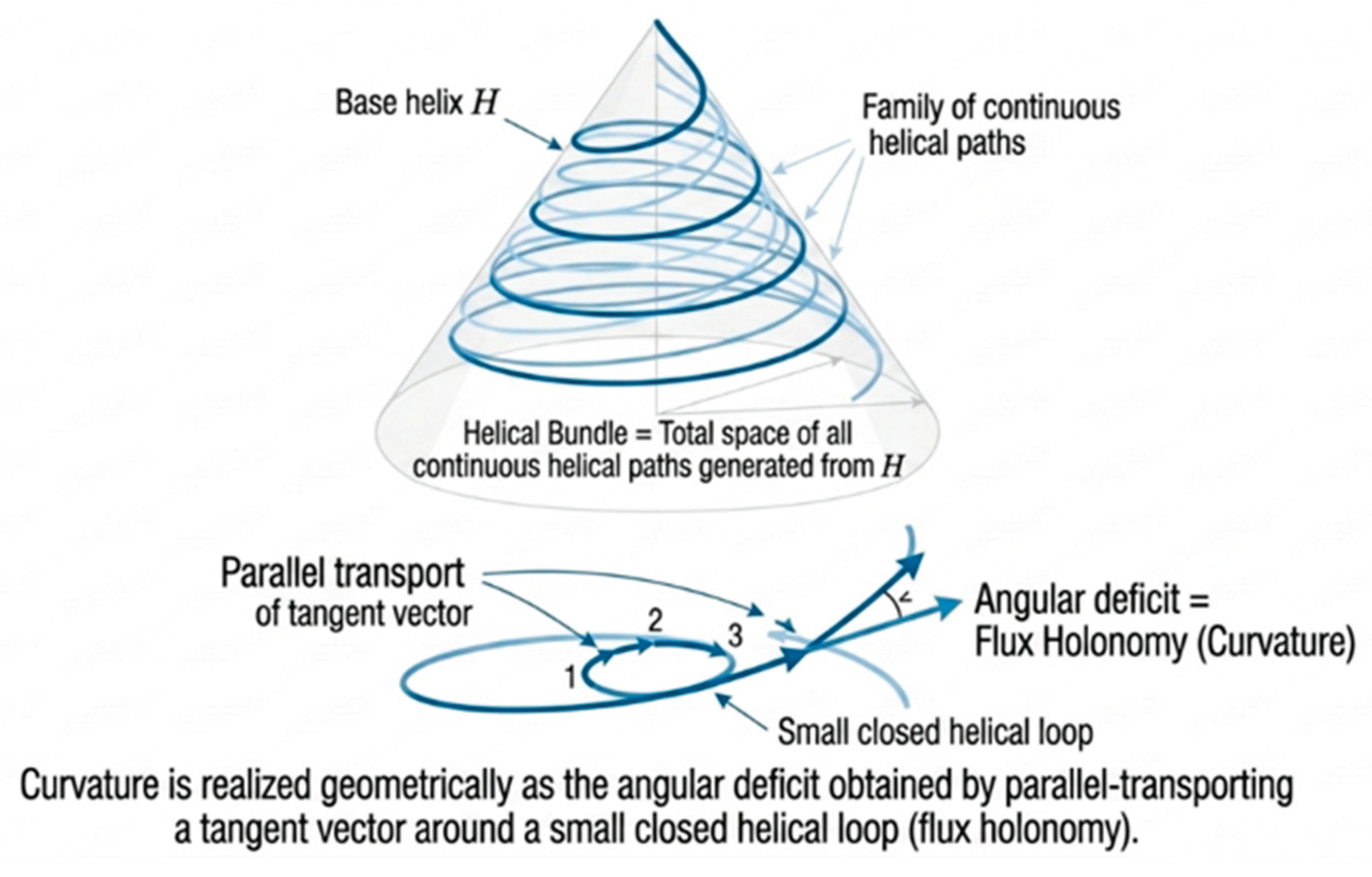
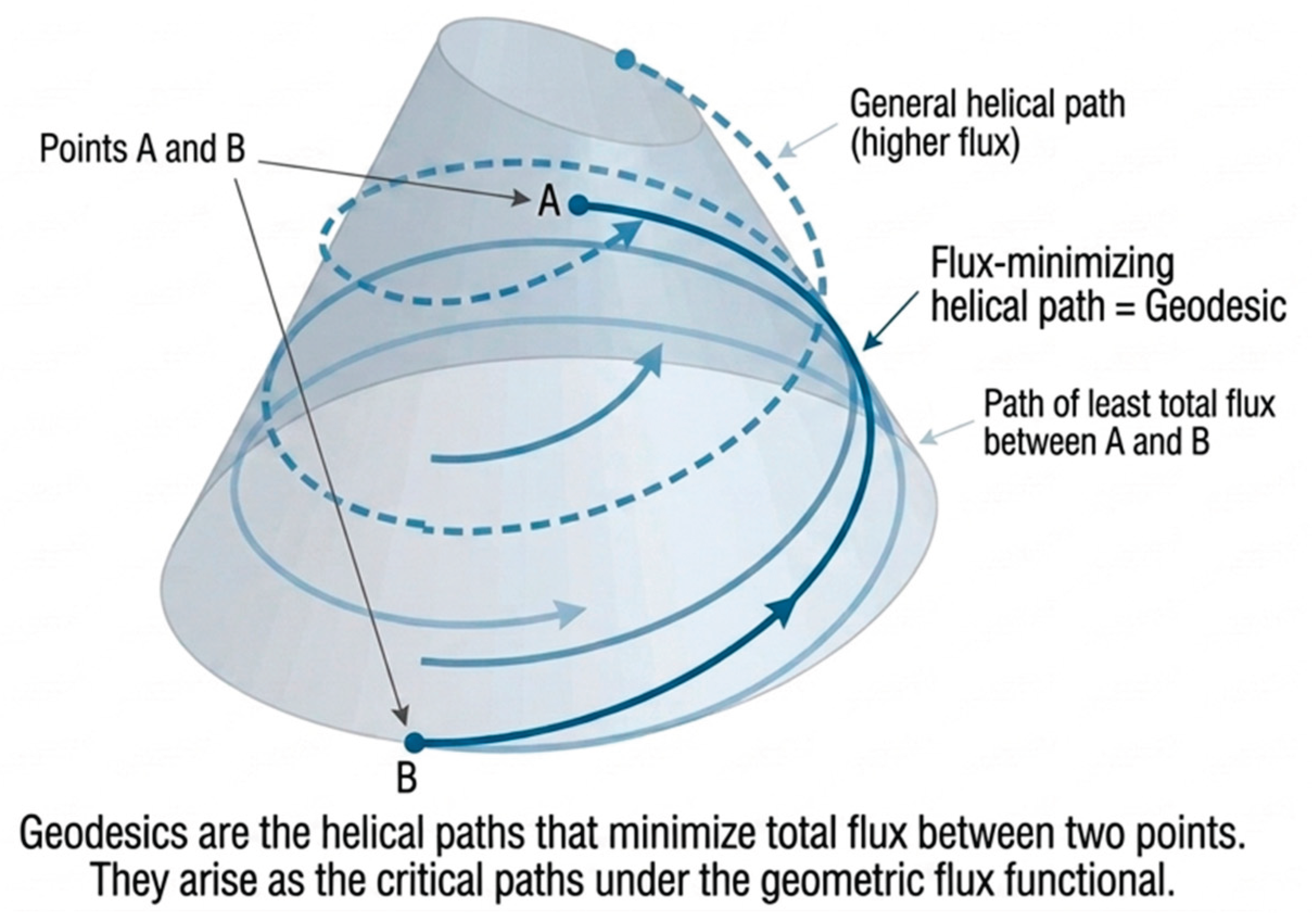
The principal structures of differential geometry are recovered as pure geometric constructions from the non-proper Archimedean conical helix and its flux [11,33,36]. The geometric tangent bundle is obtained as the total space of all first flux derivatives of helical paths [29,33]. A Riemannian metric is defined on this bundle by the flux inner product of pairs of tangent vectors [35,36]. Parallel transport of tangent vectors along helical paths is realized by continuous displacement that preserves flux length and relative angle under the six operations; the infinitesimal generator of this transport yields the geometric covariant derivative [34,36]. Curvature appears as the flux holonomy obtained by parallel-transporting a tangent vector around a small closed helical loop [36,46]. Geodesics are identified with the helical paths that minimize total flux length, equivalently characterized as the paths whose unit tangent is parallel-transported along itself [35,36,48]. Finally, the Laplace–Beltrami operator is obtained as the geometric divergence of the geometric gradient and is shown to coincide with the orthogonal projection of the helical operator ${\mathsf{\Delta }}_H$ [35,36,43]. All of these structures remain strictly inside the pure geometry of the helix and the three axioms [29].

Theorem 58 (Geometric Tangent Bundle). The geometric tangent bundle of the helical bundle (or of the recovered plane) is the total space of all first flux derivatives (geometric tangents) of helical paths. Each fiber consists of the tangent vectors at a given point, and the natural projection sends each tangent vector to its base point [29,33].

Proof of Theorem 58.

• At every point $p$ of the helical bundle there exist helical paths passing through $p$ (Theorem 33) [11,33].
• The first flux derivative of any such path at $p$ is a geometric tangent vector at $p$ (Theorem 47) [29,33].
• The collection of all these tangent vectors forms a vector space (by geometric addition and scalar multiplication of flux lengths) [7,33].
• The total space of all such tangent vectors, together with the natural projection to the base point, is the geometric tangent bundle [33].
• By G1 the construction is unique up to geometric equivalence [12,33].

This proves Theorem 58. □

Theorem 59 (Riemannian Metric from Flux Inner Product). The Riemannian metric on the geometric tangent bundle is the flux inner product of two tangent vectors: the geometric product of their flux lengths with the cosine of the included angle determined by the helical geometry [24,53,54].

Proof of Theorem 59.

• Let $u$ and $v$ be two geometric tangent vectors at the same point (Theorem 58) [33].
• Their flux lengths are well-defined positive quantities (or zero) [36].
• The included angle between them is the geometric angle formed by the corresponding helical directions (Theorem 9 and 24) [5,11].
• The product of the two flux lengths with the cosine of that angle is a geometric scalar (Theorems 19 and 20).
• This scalar is bilinear, symmetric, and positive-definite on non-zero vectors (by G3 and the properties of flux).
• The resulting bilinear form is the pure geometric Riemannian metric [36].

This proves Theorem 59. □

Theorem 60 (Covariant Derivative from Helical Parallel Transport). Parallel transport of a tangent vector along a helical path is the unique continuous displacement of the vector that preserves its flux length and its relative angle with respect to the helical direction under continuous coiling and extension. The covariant derivative is the infinitesimal generator of this parallel transport [34,35,36].

Proof of Theorem 60.

• Let $\gamma$ be a helical path and $u$ a tangent vector at the initial point of $\gamma$.
• Displace $u$ continuously along $\gamma$ by the Grow, Coil, and Extend operations so that the flux length of $u$ and the angle it makes with the tangent of $\gamma$ remain constant [11,36].
• Uniqueness: the Riemannian connection is the unique metric-compatible torsion-free connection [36].
• The resulting vector field along $\gamma$ is the parallel transport of $u$ [36].
• The infinitesimal rate of change of a vector field under this transport is the geometric covariant derivative along $\gamma$ [34,36].
• The construction is compatible with the Riemannian metric (Theorem 59) and is therefore metric-compatible [36].

This proves Theorem 60. □

Theorem 61 (Curvature as Flux Holonomy). The geometric curvature of the helical bundle (or of the recovered plane) is the flux holonomy obtained by parallel-transporting a tangent vector around a small closed helical loop: the angular deficit (or excess) of the transported vector is the pure geometric measure of curvature [36,46].

Proof of Theorem 61.

• Let $\gamma$ be a small closed helical loop based at a point $p$ [36].
• Take a tangent vector $u$ at $p$ and parallel-transport it around $\gamma$ by the continuous operations of $H$ (Theorem 60) [36].
• Upon return to $p$ the transported vector differs from the original $u$ by a geometric angle (or a flux deficit) [46].
• This angular deficit is independent of the particular vector chosen (up to scaling) and of the particular parametrization of the loop (by G1 and congruence).
• The resulting holonomy is the pure geometric curvature associated with the infinitesimal surface enclosed by $\gamma$.
• The construction is intrinsic to the helical geometry.

This proves Theorem 61. □

Figure 23. Curvature as Flux Holonomy.

Figure 23. Curvature as Flux Holonomy.

Theorem 62 (Geodesics as Flux-Minimizing Helical Paths). A geodesic is a helical path that minimizes (or extremizes) the total flux length between its endpoints. Equivalently, it is a path whose geometric tangent is parallel-transported along itself (vanishing covariant acceleration) [45,53,54].

Proof of Theorem 62.

• Let $\gamma$ be a helical path connecting two points.
• Its total flux length is the geometric integral of its speed (Theorem 48) [30,36].
• By the geometric calculus of variations (Theorem 53) the first variation of this length vanishes if and only if the covariant derivative of the unit tangent along $\gamma$ is zero (Theorem 60) [36,48].
• Paths satisfying this condition are precisely the flux-minimizing (or critical) helical paths [53,54].
• Existence of geodesics between sufficiently close points follows from the Method of Exhaustion and the completeness of the geometric continuum (Theorems 42 and 54) [30,36].
• Uniqueness (locally) follows from the uniqueness of the helical flow (Theorem 3 and G1).

This proves Theorem 62. □

Figure 24. Geodesics as Flux-Minimizing Helical Paths.

Figure 24. Geodesics as Flux-Minimizing Helical Paths.

Theorem 63 (Laplace-Beltrami Operator as Divergence of Gradient). The Laplace-Beltrami operator on the helical bundle (or on the recovered plane) is the geometric divergence of the geometric gradient. It coincides with the orthogonal projection (shadow) of the helical operator ${\Delta }_H$ onto the base geometry [35,36,43].

Proof of Theorem 63.

• The geometric gradient of a flux-valued function is the unique tangent vector that represents the first directional fluxions with respect to the Riemannian metric (Theorems 47 and 59) [36].
• The geometric divergence of a vector field is the infinitesimal flux expansion of that field under the continuous operations of $H$ [31,36].
• The composition “divergence of gradient” is a second-order geometric operator [36,43].
• By the earlier identification of the Laplacian as the shadow of ${\mathsf{\Delta }}_H$ (Theorem 37) this composition coincides with that shadow [43].
• The resulting operator is the pure geometric Laplace-Beltrami operator; it is self-adjoint with respect to the flux measure (Theorem 56) and is intrinsically generated by the helical geometry [31,43].

This proves Theorem 63. □

11. Sets, Functions, and Wave-Particle Duality

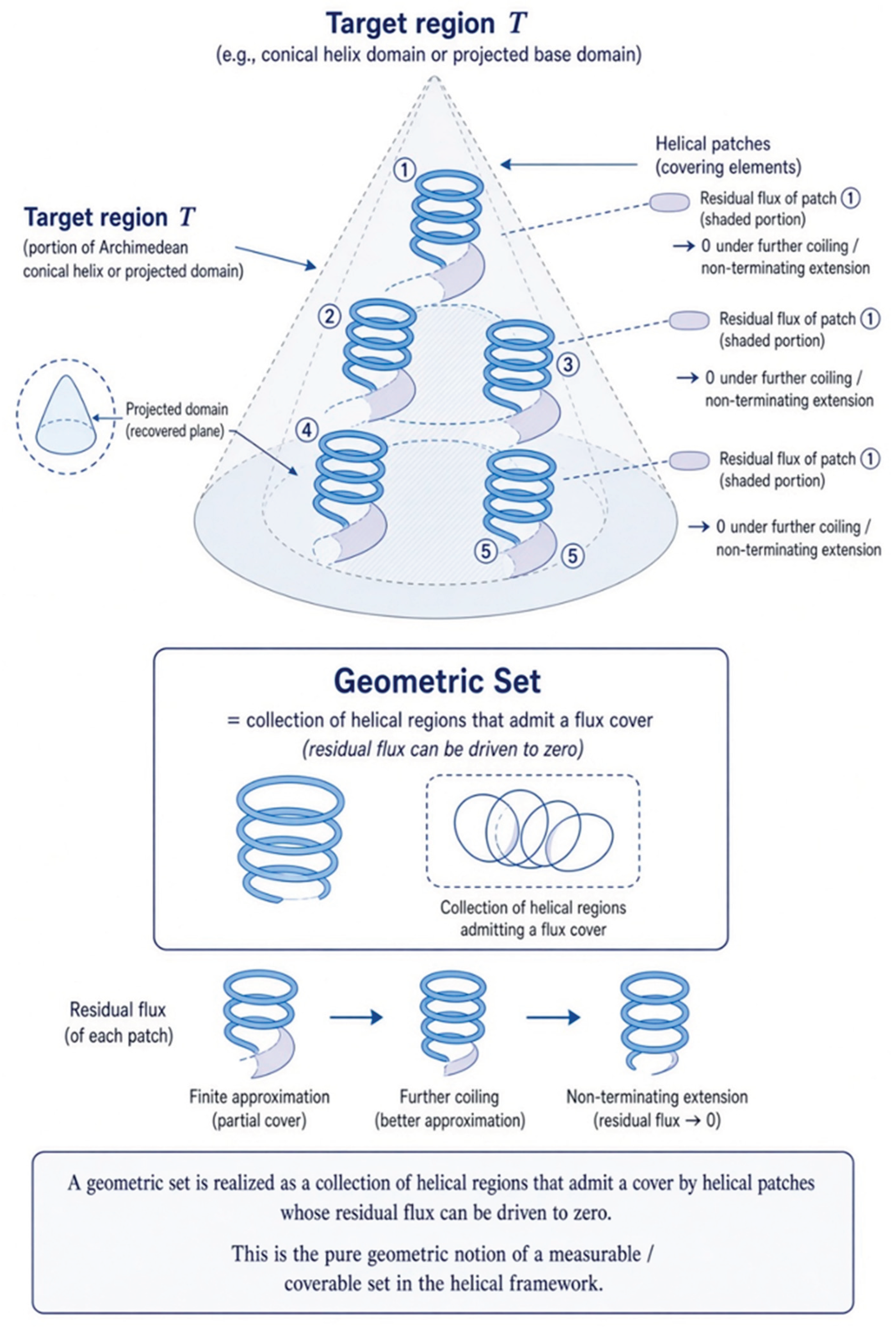
The final pure geometric structures of the present work are obtained from the non-proper Archimedean conical helix [11]. Geometric sets are realized as collections of points or helical paths that admit covers by helical regions whose residual flux can be driven to zero under the method of exhaustion [10,31,37]. Geometric functions are defined as maps between such sets that send helical paths to helical paths while preserving total flux up to congruence [2,9,37]; the composition of geometric functions remains flux-preserving. The same helix is then shown to embody a geometric form of wave–particle duality: its continuous aspect appears as the unbroken non-terminating coiling, radial growth, and flux flow, while its discrete aspect appears as the succession of irreducible cycles counted by the successor operation [2,11,38]. These two complementary faces are exhaustive under the six intrinsic operations and the three axioms, and no further geometric feature of the helix lies outside their joint scope [4]. With these constructions the pure geometric development is complete.

Theorem 64 (Geometric Sets as Flux Covers). A geometric set is a collection of points on the recovered plane (or of helical paths in the helical bundle) that admits a cover by helical regions whose residual flux can be driven to zero by the Method of Exhaustion. Equivalently, it is any region that can be exhausted by successive multi-coil figures under G1 [10,31,37].

Proof of Theorem 64.

• Let $S$ be a collection of points or helical paths.
• By the geometric measure theory already constructed (Theorem 56) every helical region carries a definite flux [15,31].
• If there exists a sequence of multi-coil helical covers of $S$ such that the residual flux outside the covers tends to zero under non-terminating extension (Theorems 17 and 42), then $S$ is geometrically measurable and is called a geometric set [10,31].
• The construction is independent of the particular sequence of covers chosen (by G1 and G3) [31].
• Thus geometric sets are precisely the flux-coverable collections arising from the helix [2,37].

This proves Theorem 64. □

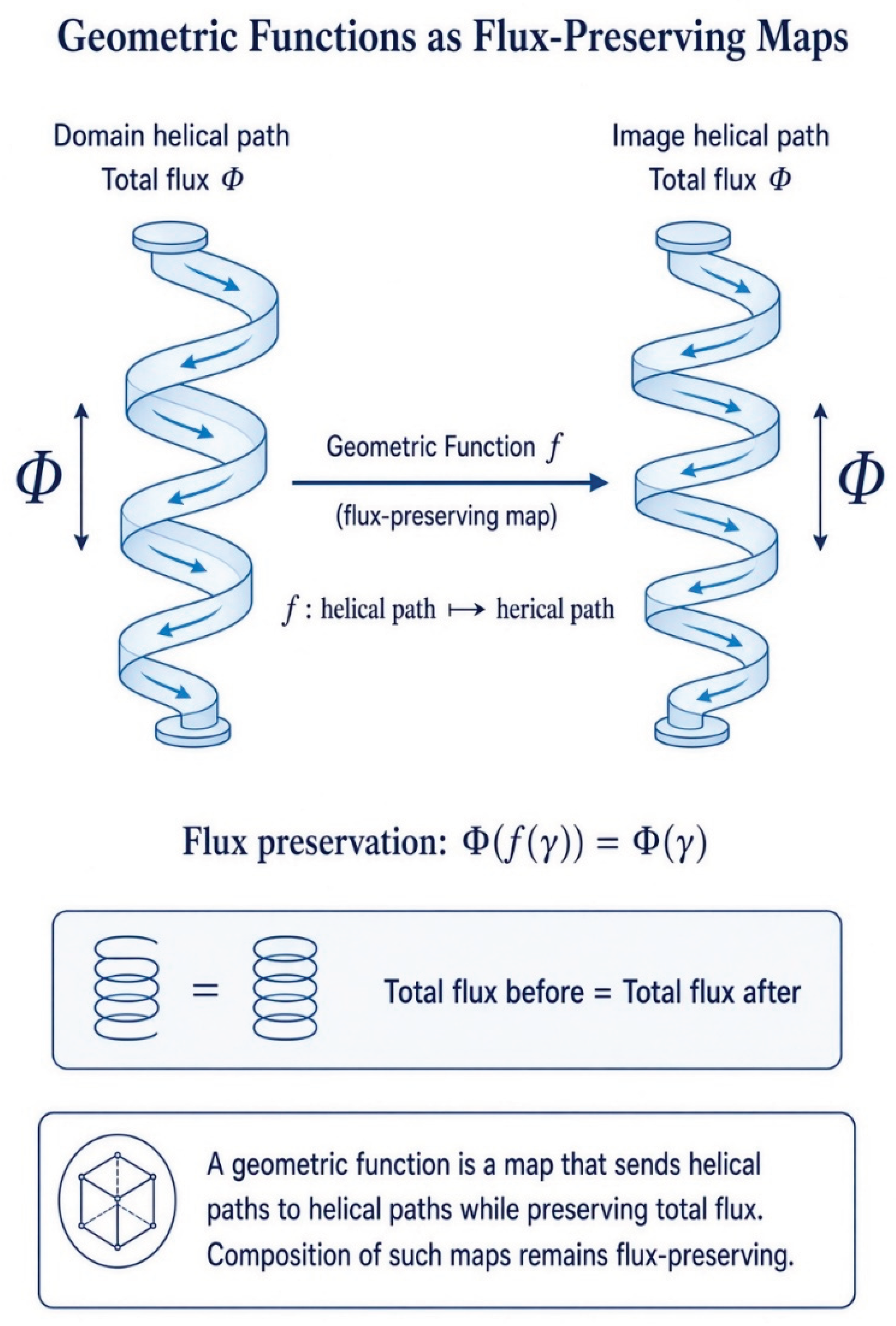
Theorem 65 (Geometric Functions as Flux-Preserving Maps). A geometric function is a map between geometric sets that sends helical paths to helical paths (or flux data to flux data) while preserving total flux up to congruence. Composition of geometric functions remains flux-preserving [2,9,37].

Proof of Theorem 65.

• Let $S$ and $T$ be geometric sets (Theorem 64) [37].
• A map $f:S\to T$ is geometric when it is realized by a finite composition of the six primitive operations (or by the continuous flow of $H$) and the total flux of any helical path is preserved under $f$(G3) [12,15].
• Congruence of the image path with the original path (up to the action of the operations) is guaranteed by the uniqueness of $H$ (Theorem 3), Theorem 2 and Theorem 9 [7].
• The composition of two such maps is again realized by a composition of the six operations and therefore remains flux-preserving [9,37].
• Consequently the geometric functions form a category [3,9,37] under composition whose morphisms are the flux-preserving maps of the helical geometry.

This proves Theorem 65. □

Figure 25. Flux as Geometric Measure.

Figure 25. Flux as Geometric Measure.

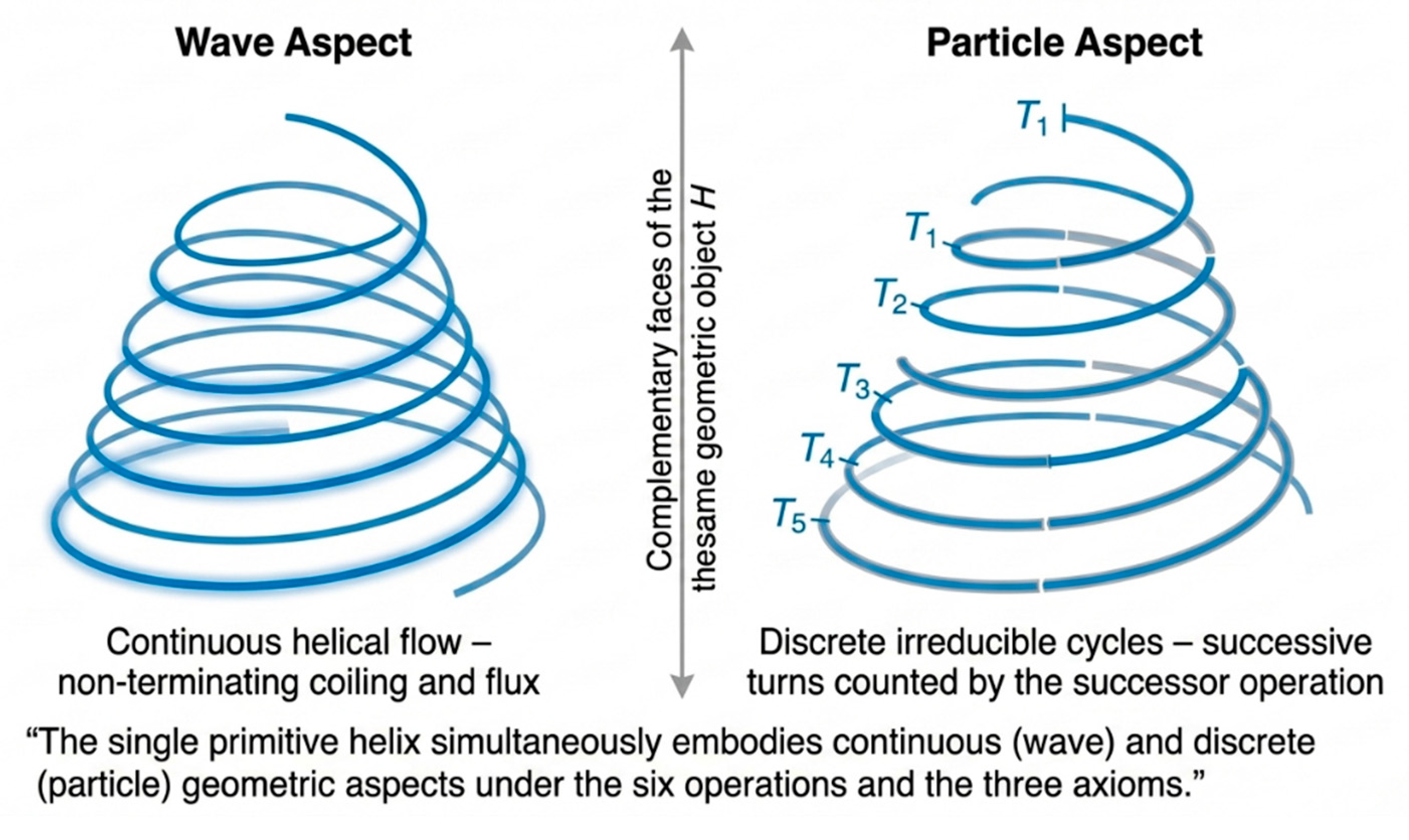
Theorem 66 (Wave-Particle Duality Embodied by$H$). The non-proper Archimedean conical helix $H$ simultaneously embodies a continuous wave aspect and a discrete particle aspect. The wave aspect is the non-terminating continuous coiling, radial growth, and flux flow; the particle aspect is the succession of irreducible cycles (turns) counted by the successor function. The two aspects are complementary faces of the same geometric object under G1–G3 [2,11,38].

Proof of Theorem 66.

• Continuous application of the Coil, Grow, and Extend operations produces an unbroken helical flow whose frequency, phase, and flux density vary continuously (Theorems 34 and 44). [11,23] This is the wave aspect of $H$ [38].
• The same helix admits a discrete decomposition into successive complete turns (Theorem 32) whose lengths are the irreducible cycles (Theorem 26) [2,13]. These indivisible turns are the particle aspect of $H$
• The two descriptions are related by the continuous versus discrete modes of the identical six operations: every continuous path can be partitioned into discrete coils, and every discrete succession of coils can be smoothed into a continuous helical flow [11].
• By G1–G3 the two aspects are complementary and exhaustive: there is no geometric feature of $H$ that is neither wave-like nor particle-like.
• Therefore the single geometric object $H$ embodies wave-particle duality in pure geometric form [11,38].

Figure 26. Geometric Functions as Flux-Preserving Maps.

Figure 26. Geometric Functions as Flux-Preserving Maps.

This proves Theorem 66. □

Figure 27. Wave–Particle Duality Embodied by the Non-Proper Archimedean Conical Helix $H.$

Figure 27. Wave–Particle Duality Embodied by the Non-Proper Archimedean Conical Helix $H.$

12. Discussion

The present work establishes that a single geometric object—the non-proper Archimedean conical helix $H$—together with six intrinsic operations and three pure geometric axioms, is sufficient to generate a coherent cascade of classical and modern mathematical structures [4,11]. Points, lines, circles, congruence, parallelism [5,6,7], the constants $\pi$ and $\varphi$ [10,22], the imaginary unit [28], the natural numbers [2], the primes, addition and multiplication [7], flux as measure [31], geodesics [36], curvature as holonomy [46], and the wave–particle duality of the helix [11,38] itself all appear as canonical geometric shadows of this one primitive figure [4]. The development remains internal to pure geometry: no external numerical, set-theoretic, or analytic primitives are introduced at the base [2,6].

The principal significance of the construction lies in its geometry-first character. Classical foundations typically begin with points, lines, and incidence axioms, or with sets and membership [2,5,6]. Here the opposite direction is taken. The familiar Euclidean primitives and the arithmetic structures that rest upon them are recovered rather than assumed [7]. The helix supplies both a continuous aspect (non-terminating coiling and flux) and a discrete aspect (successive irreducible turns) [2,11], so that the wave–particle duality is not an added interpretation but an intrinsic geometric feature of the generating object. In this sense the work offers a concrete illustration of how a single, visually and operationally rich figure can serve as a generative nucleus for a substantial portion of mathematics [4].

The scope of the present paper is deliberately limited to the pure geometric layer. The cascade is carried through the recovery of classical geometry [5,6,7,8,19,42], the fundamental constants [10,20,21,22,28], elementary arithmetic operations [4,40], flux and measure [31], the principal differential-geometric notions [33,36,43,46,52] (geodesics, curvature, the helical operator and its Laplacian and Sturm–Liouville shadows), and the wave–particle duality [11]. Later categorical, type-theoretic, and set-theoretic reconstructions—while naturally suggested by the same geometric substrate—are left for subsequent work [4,37,40,41]. This limitation is methodological rather than absolute: the geometric foundation is offered as a self-contained first stage whose further extension remains open.

Several directions present themselves immediately. The most direct is the systematic development of the geometric sets and geometric functions already indicated in the later theorems, followed by the construction of the associated topos and the extraction of its internal logic [4,9,37,40]. A second direction is the detailed spectral analysis of the helical operator ${\mathsf{\Delta }}_H$ [39,43,54] and the precise geometric origin of the Euler-product structure encoded in the grand-partition function. A third is the examination of whether the same helix, under suitable multi-helix or bundled configurations, can generate higher-dimensional differential geometry and the classical operators of mathematical physics [34,47,56]. Each of these extensions remains grounded in the same primitive object and the same three axioms.

In summary, the non-proper Archimedean conical helix is shown to be a surprisingly fertile geometric generator [4,11]. The structures recovered from it are not imposed from outside but arise by the repeated application of a small set of purely geometric operations under three transparent axioms [7,36]. The resulting cascade demonstrates that a geometry-first foundation is possible at least through the classical and differential-geometric layers of mathematics [5,36], and it invites a systematic exploration of how much further the same generative principle can be carried.

13. Conclusions

The non-proper Archimedean conical helix $H$, equipped with six intrinsic geometric operations and three pure geometric axioms, has been shown to generate a coherent cascade of mathematical structures. Classical geometric primitives, the fundamental constants $\pi$ and $\varphi$, the imaginary unit, the natural numbers and the primes, the elementary arithmetic operations, flux as geometric measure, geodesics, curvature as holonomy, the helical operator and its Laplacian and Sturm–Liouville shadows, and the wave–particle duality of the helix itself all arise as canonical geometric consequences of this single primitive figure.

The development remains internal to pure geometry. No external numerical, set-theoretic or analytic starting points are required. The continuous and discrete aspects of mathematics appear as complementary faces of the same object, and the familiar structures of Euclidean geometry and elementary arithmetic are recovered rather than postulated.

The present work is limited to the pure geometric layer of the cascade. The further extraction of categorical, type-theoretic and set-theoretic frameworks from the same geometric substrate is left open. Within the domain it addresses, however, the construction demonstrates that a geometry-first foundation is possible and that a single, operationally rich figure can serve as a generative nucleus for a substantial portion of classical and differential geometry.

The helix therefore stands as a concrete example of how far pure geometric generation can be carried when the starting object and the admissible operations are chosen with sufficient care.

References

- Aiguier, M. From category theory to categorical logic [Lecture slides]. Center for Advanced Studies, Institut de Mathématiques de Roumanie. 2024. Available online: https://ctta.igrothendieck.org/wp-content/uploads/2024/09/Slides_AiguierMarc.pdf.
- Lawvere, F. W. An elementary theory of the category of sets. Proc. Natl. Acad. Sci. USA 1964, 52(6), 1506–1511. [Google Scholar] [CrossRef] [PubMed]
- Lawvere, F. W. The category of categories as a foundation for mathematics. In Proceedings of the Conference on Categorical Algebra; Eilenberg, S., Harrison, D. K., Mac Lane, S., Röhrl, H., Eds.; Springer, 1966; pp. 1–20. [Google Scholar] [CrossRef]
- Caramello, O. The unification of mathematics via topos theory. nLab. 2010. Available online: https://pages.jh.edu/rrynasi1/FoundationsOFMath/Literature/Caramello2010TheUnificationOfMathematicsViaToposTheory.pdf.
- Euclid. The thirteen books of Euclid’s Elements, 2nd ed.; Heath, T. L., Translator; Dover, 1956; Vols. 1–3. [Google Scholar]
- Hilbert, D. The foundations of geometry; Townsend, E. J., Translator; Open Court Publishing Company, 1902. (Original work published 1899). [Google Scholar]
- Hartshorne, R. Geometry: Euclid and beyond; Springer, 2000. [Google Scholar]
- Pasch, M. Vorlesungen über neuere Geometrie [Lectures on newer geometry]; B. G. Teubner, 1882. [Google Scholar]
- Makkai, M.; Reyes, G. E. First order categorical logic: Model-theoretical methods in the theory of topoi and related categories. In Lecture Notes in Mathematics; Springer, 1977; Vol. 611. [Google Scholar] [CrossRef]
- Archimedes. Measurement of a circle. In The works of Archimedes; Heath, T. L., Ed.; Heath, T. L., Translator; Cambridge University Press, 1897; pp. 91–98, (Original work published ca. 250 BCE). [Google Scholar]
- do Carmo, M. P. Differential geometry of curves and surfaces; Prentice-Hall, 1976. [Google Scholar]
- Kolář, I.; Michor, P. W.; Slovák, J. Natural operations in differential geometry; Springer, 1993. [Google Scholar]
- Cavalieri, B. Geometria indivisibilibus continuorum nova quadam ratione promota; Bologna, 1635. [Google Scholar]
- Andersen, K. Cavalieri’s method of indivisibles. Arch. Hist. Exact. Sci. 1985, 31, 291–367. [Google Scholar] [CrossRef]
- Tchuiaga, S. Hofer-like geometry and flux theory. J. Dyn. Syst. Geom. Theor. 2021, 19(2), 227–270. [Google Scholar] [CrossRef]
- Fellin, G.; Negri, S.; Orlandelli, E. Glivenko sequent classes and constructive cut elimination in geometric logics. Arch. Math. Log. 2023, 62, 657–688. [Google Scholar] [CrossRef]
- Negri, S. Glivenko sequent classes in the light of structural proof theory. Arch. Math. Log. 2016, 55(3–4), 461–473. [Google Scholar] [CrossRef]
- Negri, S.; von Plato, J. Structural proof theory; Cambridge University Press, 2001. [Google Scholar] [CrossRef]
- Greenberg, M. J. Old and new results in the foundations of elementary plane Euclidean and non-Euclidean geometries. Am. Math. Mon. 2010, 117(3), 198–219. [Google Scholar] [CrossRef]
- Janjić, M. Geometrical definition of π and its approximations by nested radicals. Teach. Math. 2008, 11(1), 25–34. [Google Scholar]
- Nathan, J. A. π and arc-length. arXiv. 2021. Available online: https://arxiv.org/abs/2104.09788.
- Livio, M. The golden ratio: The story of phi, the world’s most astonishing number; Broadway Books, 2002. [Google Scholar]
- Newton, I. The method of fluxions and infinite series; with its application to the geometry of curve-lines; Colson, J., Translator; Henry Woodfall, 1736. [Google Scholar]
- Barrow, I. Lectiones geometricae; London, 1670. [Google Scholar]
- Gregory, J. Geometriae pars universalis; Padua, 1668. [Google Scholar]
- Roy, R. Geometric calculus. In Sources in the development of mathematics: Series and products from the fifteenth to the twenty-first century (Chap. 7).; Cambridge University Press, 2011. [Google Scholar]
- Boyer, C. B. The history of the calculus and its conceptual development; Dover, 1959. [Google Scholar]
- Needham, T. Visual complex analysis, 25th anniversary ed.; Oxford University Press, 2023. (Original work published 1997). [Google Scholar]
- Spivak, M. Calculus on manifolds: A modern approach to classical theorems of advanced calculus; Addison-Wesley, 1965; p. 50. [Google Scholar]
- Burago, D.; Burago, Y.; Ivanov, S. A course in metric geometry; American Mathematical Society, 2001; Vol. 33. [Google Scholar]
- Federer, H. Geometric measure theory; Springer, 1969. [Google Scholar]
- Federer, H.; Fleming, W. H. Normal and integral currents. Ann. Math. 1960, 72(3), 458–520. [Google Scholar] [CrossRef]
- Lee, J. M. Introduction to smooth manifolds, 2nd ed.; Springer, 2013. [Google Scholar]
- Spivak, M. A comprehensive introduction to differential geometry, 3rd ed.; Publish or Perish, 1999; Vols. 1–5. [Google Scholar]
- do Carmo, M. P. Riemannian geometry; Birkhäuser, 1992. [Google Scholar]
- Lee, J. M. Introduction to Riemannian manifolds, 2nd ed.; Springer, 2018. [Google Scholar] [CrossRef]
- Mac Lane, S.; Moerdijk, I. Sheaves in geometry and logic: A first introduction to topos theory; Springer-Verlag, 1992. [Google Scholar]
- Claerbout, J. F. Multidimensional recursive filters via a helix. Geophysics 1998, 63(5), 1532–1541. [Google Scholar] [CrossRef]
- Kubota, Y.; Ludewig, M.; Thiang, G. C. Delocalized spectra of Landau operators on helical surfaces. Commun. Math. Phys. 2022, 395(3), 1211–1242. [Google Scholar] [CrossRef]
- Johnstone, P. T. Sketches of an elephant: A topos theory compendium (Vols. 1–2); Oxford University Press, 2002. [Google Scholar]
- Kock, A. Synthetic differential geometry, 2nd ed.; Cambridge University Press, 2006. [Google Scholar]
- Greenberg, M. J. Euclidean and non-Euclidean geometries: Development and history, 4th ed.; W. H. Freeman and Company, 2008. [Google Scholar]
- Chavel, I. Eigenvalues in Riemannian geometry; Academic Press, 1984. [Google Scholar]
- Guicciardini, N. Isaac Newton on mathematical certainty and method; MIT Press, 2009. [Google Scholar]
- Hestenes, D.; Sobczyk, G. Clifford algebra to geometric calculus: A unified language for mathematics and physics; Springer, 1984. [Google Scholar] [CrossRef]
- Ambrose, W.; Singer, I. M. A theorem on holonomy. Trans. Am. Math. Soc. 1953, 75(3), 428–443. [Google Scholar] [CrossRef]
- O’Neill, B. Semi-Riemannian geometry with applications to relativity. In Pure and Applied Mathematics; Academic Press, 1983; Vol. 103. [Google Scholar]
- Jost, J.; Li-Jost, X. Calculus of variations; Cambridge University Press, 1998. [Google Scholar]
- Coxeter, H. S. M. Introduction to geometry, 2nd ed.; John Wiley & Sons, 1989. (Original work published 1961). [Google Scholar]
- Hurwitz, A. Über die angenäherte Darstellung der Irrationalzahlen durch rationale Brüche. Math. Ann. 1891, 39(2), 279–284. [Google Scholar]
- Ford, L. R. A geometrical proof of a theorem of Hurwitz. Proc. Edinb. Math. Soc. 1916, 35, 59–65. [Google Scholar] [CrossRef]
- Balestro, V.; Martini, H.; Teixeira, R. A new geometric view on Sturm–Liouville eigenvalue problems. Monatshefte Für Math. 2019, 190, 213–236. [Google Scholar] [CrossRef]
- Olver, P. J. Applications of Lie groups to differential equations. In Graduate Texts in Mathematics, 2nd ed.; Springer, 1993; Vol. 107. [Google Scholar]
- Ariturk, S. An annulus and a half-helicoid maximize Laplace eigenvalues. J. Spectr. Theory 2018, 8(2), 315–346. [Google Scholar] [CrossRef] [PubMed]
- Abraham, R.; Marsden, J. E. Foundations of mechanics, 2nd ed.; Benjamin/Cummings, 1978. [Google Scholar]
- Bonito, A.; Nochetto, R. H. (Eds.) Geometric partial differential equations – Part I. In Handbook of Numerical Analysis; Elsevier, 2020; Vol. 21. [Google Scholar]
Disclaimer/Publisher’s Note: The statements, opinions and data contained in all publications are solely those of the individual author(s) and contributor(s) and not of MDPI and/or the editor(s). MDPI and/or the editor(s) disclaim responsibility for any injury to people or property resulting from any ideas, methods, instructions or products referred to in the content. |
© 2026 by the author. Licensee MDPI, Basel, Switzerland. This article is an open access article distributed under the terms and conditions of the Creative Commons Attribution (CC BY) license.
Copyright: This open access article is published under a Creative Commons CC BY 4.0 license, which permit the free download, distribution, and reuse, provided that the author and preprint are cited in any reuse.