

Submitted:
28 August 2026
Posted:
28 August 2026
You are already at the latest version
Abstract
The data-centric artificial intelligence (AI) paradigm posits that improvements to training data quality yield greater performance increases compared to changes to model architecture; however, the claim is currently supported by case studies and demonstrations rather than controlled experiments. The experiments used five corpora with varying amounts of label noise (0.0% to 54.7%) and three distinct model architectures (LinearSVC, DistilBERT, and RoBERTa), resulting in 135 total experimental conditions based on the combination of two remediation strategies applied across five thresholds. All conditions were assessed via five-fold stratified cross-validation. Label errors within the five corpora were identified using confident learning (a probabilistic approach to flagging potentially mislabeled training examples by comparing predicted class probabilities with observed labels). The identification of label errors were validated independently against the CIFAR-N benchmark prior to conducting downstream analyses. To aid in connecting the results of this research to practice, cost-performance Pareto frontiers were created for each of four distinct levels of annotation costs. Lastly, a theoretical framework was developed to explain the observed architecture-noise interaction patterns.
Keywords:
data quality
; label noise
; architecture selection
; artificial intelligence
; Pareto frontier
; confident learning
Introduction
Problem Statement
If a text classification model does not function adequately, a practitioner must determine whether to invest more resources into a larger, higher-performing architecture or whether to improve the quality of the data used to train it.
Figure 1.
Where to invest when a text classifier underperforms. Note. The two investment options a practitioner faces when a text classifier underperforms, with the tradeoffs of each. This study empirically identifies the noise conditions under which each option dominates.
Figure 1.
Where to invest when a text classifier underperforms. Note. The two investment options a practitioner faces when a text classifier underperforms, with the tradeoffs of each. This study empirically identifies the noise conditions under which each option dominates.
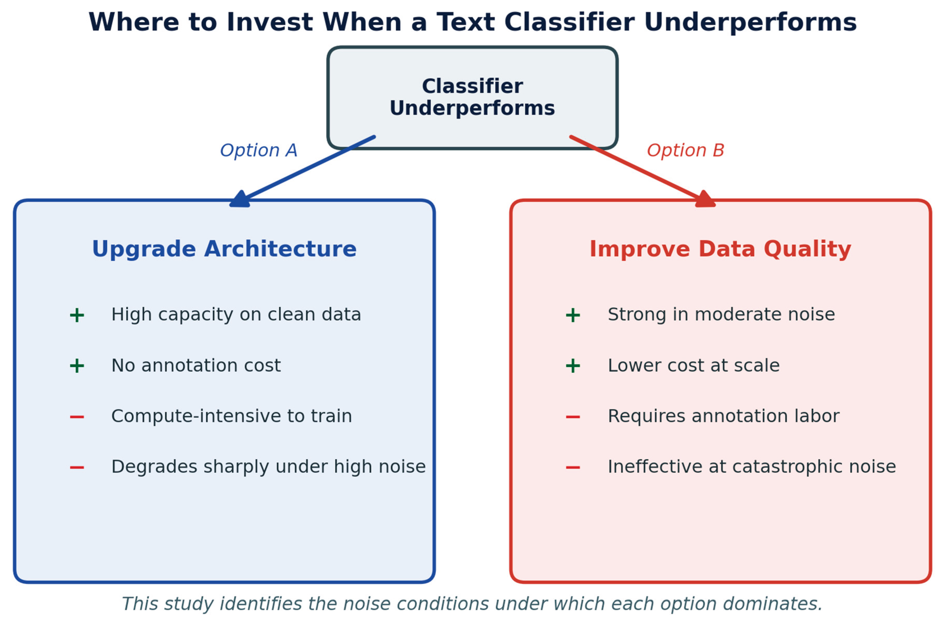
The premise of the data-centric artificial intelligence (AI) paradigm is that enhancing the quality of the training data results in greater and more consistent improvements than changing the architecture. The primary evidence supporting this paradigm is anecdotal. Existing evidence has been developed through observation and is based on a few case studies and demonstrations. In natural language processing, controlled studies that methodically vary data quality while maintaining the same architecture are currently lacking. This gap is articulated in depth in the Literature Review. To address the gap in the literature, the main research question guiding this study is: How do data quality and model architecture affect performance on text classification, under varying levels of label noise?
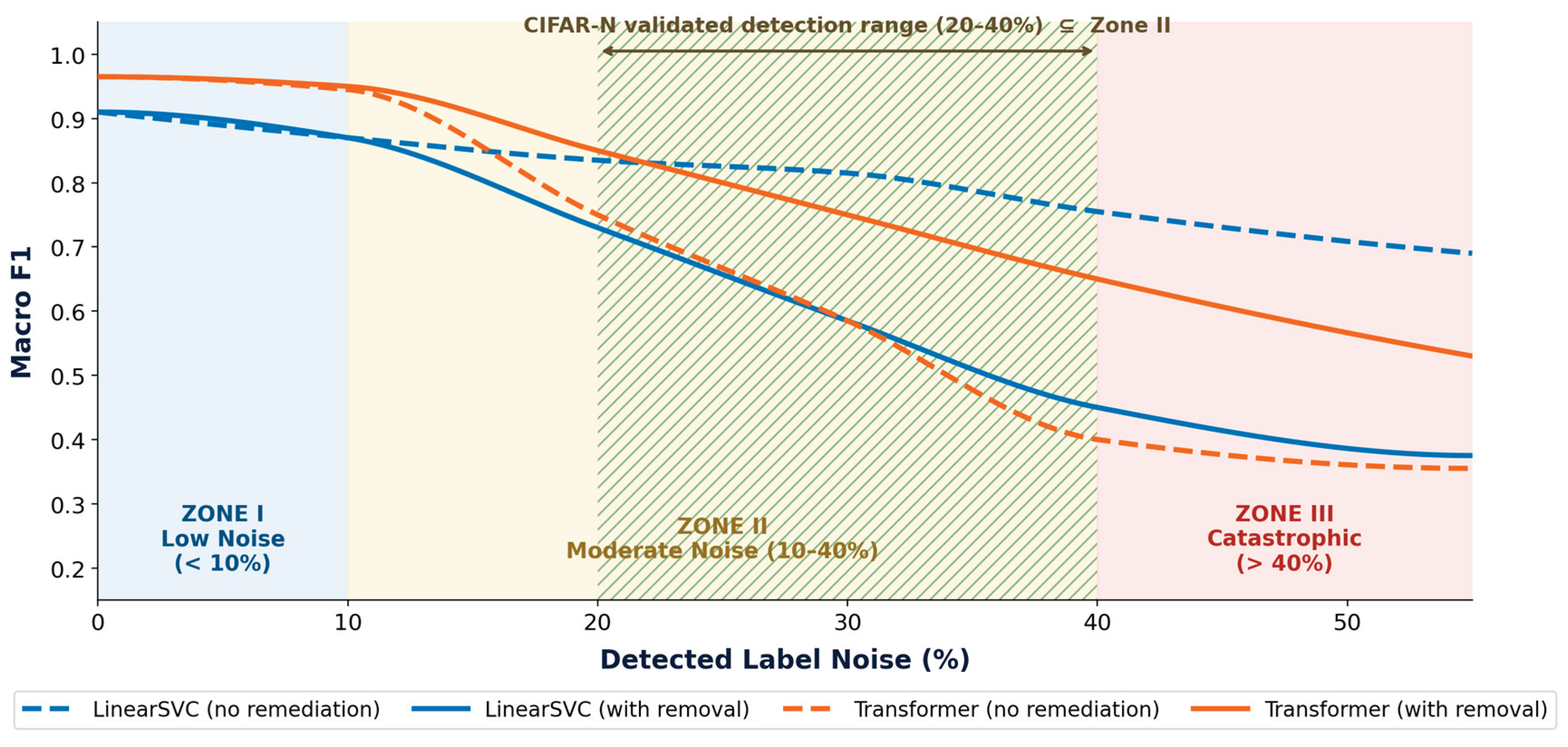
In this study, noise regimes are ranges of label-error rates that differ qualitatively in their behavioral characteristics. Low-noise conditions support clean patterns in the data. Moderate-noise conditions allow for the interaction of intervention effect and architectural type. Catastrophic noise conditions arise when there is such severe degradation of the label signal that it cannot be recovered. Relationship collapse occurs when neither an investment in data quality improvement nor an investment in architecture can return task performance to above random chance.
The research question is represented by three sub-questions:
1. In what noise regimes is the impact of data quality improvement greater than the impact of architectural upgrade?
2. In what noise regimes does the impact of architecture exceed the impact of data quality improvement?
3. In what noise regimes does relationship collapse occur, where neither architectural nor data quality intervention can help improve performance?
Figure 2.
Architectural-selection process controlled by three distinct areas of noise. Note. In Zone I (0–10% noise), Transformer architectures provide improved performance across all noise levels. In Zone II (10–40% noise), improving data quality allows for the realization of the best results from a Transformer. The architectural crossover occurs here. In Zone III (>40% noise), there is partial or complete loss of performance due to severe levels of noise. The shaded band indicates the noise range validated by the CIFAR-N dataset (20–40% noise).
Figure 2.
Architectural-selection process controlled by three distinct areas of noise. Note. In Zone I (0–10% noise), Transformer architectures provide improved performance across all noise levels. In Zone II (10–40% noise), improving data quality allows for the realization of the best results from a Transformer. The architectural crossover occurs here. In Zone III (>40% noise), there is partial or complete loss of performance due to severe levels of noise. The shaded band indicates the noise range validated by the CIFAR-N dataset (20–40% noise).
Origin of the Research Question
The basis for the research question came from an unexpected finding in a pilot study developed by Senne (2026). In this pilot study, four distinct architectures (having different numbers of parameters) were evaluated using the same corpus that exhibited a distinct linguistic structure, but none of them achieved good performance (all performed at or below chance levels). Currently, there exists an inability in the natural language processing (NLP) literature to clearly define the boundary between datasets with recoverable label signals and those that do not contain them. Therefore, a more controlled examination was completed as reported in this study. In addition to the findings of the pilot study, the design, corpora, and per-corpus statistics that produced this anomaly are reported in Appendix D.
This anomaly provides the basis of the empirical question that underpins this study. When a dataset possesses consistent linguistic structure but was labelled using non-structured methods, the degree to which systematic restoration of label errors can retrieve recoverable signal is an empirical question rather than a question of qualitative preference (Northcutt, Jiang, and Chuang 2021; Wei et al. 2022). The boundaries between datasets with recoverable signals and those without have not been defined in the NLP literature reviewed in this study. Therefore, the threshold for selecting models remains absent from that literature.
Hypotheses
The research question is decomposed into four testable hypotheses that structure the empirical work:
H1:
Catastrophic Noise Threshold: Classifier performance will fail to exceed chance-level performance for tested architecture (under all remediation threshold and remediation strategy) on corpora with detected label noise above 40%.
H2:
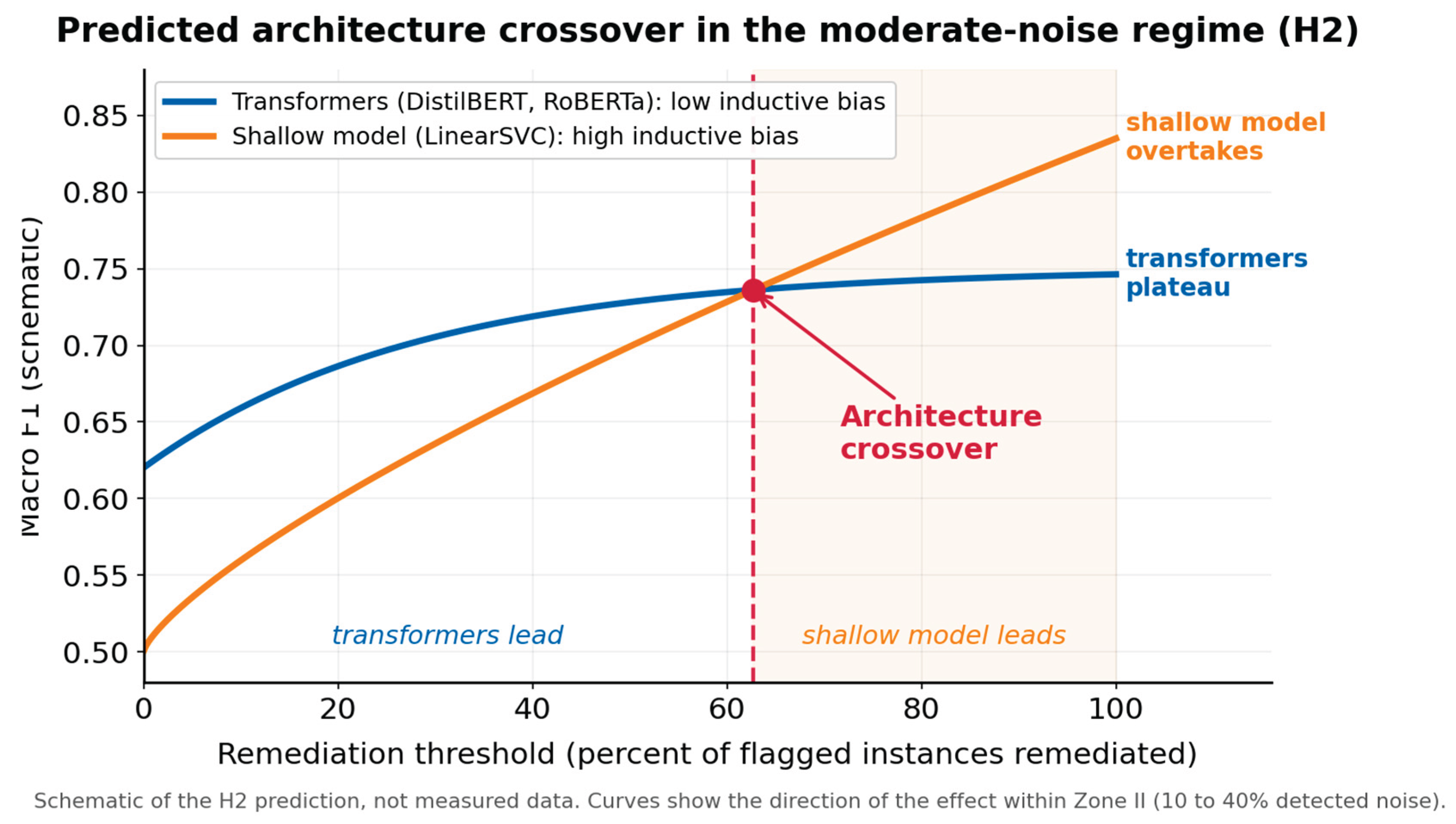
Architecture Crossover: On corpora with detected label noise between 20% and 40%, two predicted effects occur. First, for the shallow architecture (LinearSVC), the remediation via instance removal will provide the greatest performance gain compared to the transformer architectures (DistilBERT, RoBERTa). Therefore, this differential gain produces an architecture crossover, which represents a remediation threshold less than 100% at or below which shallow architecture will achieve equal or greater performance than (to) transformer(s).
Figure 3.
Predicted architecture crossover in the moderate-noise regime (H2). Note. As remediation raises training-data quality, the high-bias shallow model (LinearSVC) gains more than the low-bias transformers (DistilBERT, RoBERTa) and overtakes them at a crossover threshold below full remediation. The figure is a schematic of the prediction, not measured data.
Figure 3.
Predicted architecture crossover in the moderate-noise regime (H2). Note. As remediation raises training-data quality, the high-bias shallow model (LinearSVC) gains more than the low-bias transformers (DistilBERT, RoBERTa) and overtakes them at a crossover threshold below full remediation. The figure is a schematic of the prediction, not measured data.
H3:
(Low-Noise Architectural Hierarchy): Transformer architectures (DistilBERT, RoBERTa) will outperform shallow architectures (LinearSVC) at all remediation thresholds for corpora with detected label noise below 10%. This is consistent with the standard architectural hierarchy on clean or near-clean data.
H4:
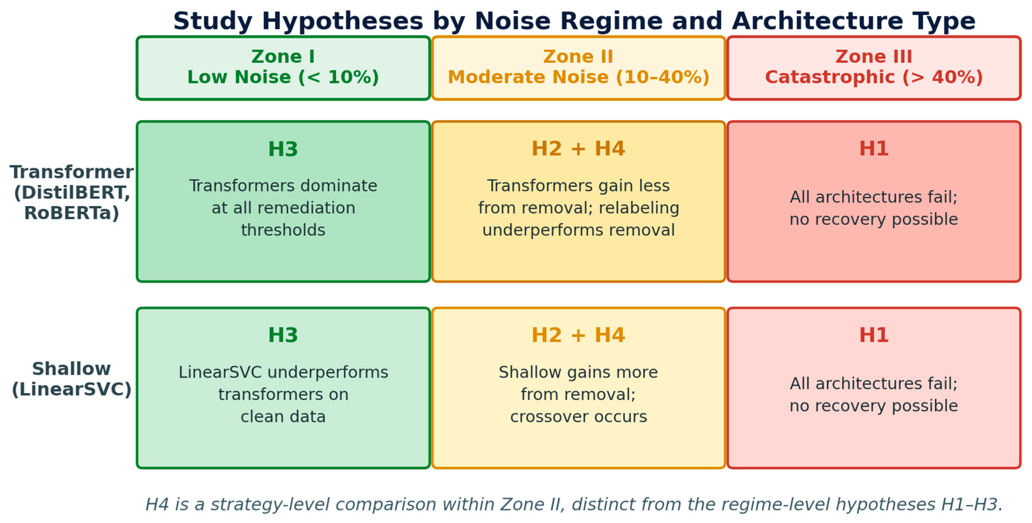
(Comparison of Remediation Strategies for Moderate Noise): The above three hypotheses characterize how different regimes exhibit certain architectural characteristics of the model on a regime level; while the H4 hypothesis attempts to address a separate question, this hypothesis is strategy-level and arose due to the moderate noise analysis (Zone II) on the two transformer architectures (10–40% of identified noise) within their respective zones. Most corpora encountered in the real world through the use of NLP applications are likely to fall within this range; this means that when a corpus has some inherent noise, there is an opportunity to remediate the noise within the corpus to improve model performance through the selection of remediation strategies. When choosing these remediation strategies within the moderate noise zone, the strategy chosen will have a direct impact on the direction and trajectory of model performance between instance removal and relabeling as suggested by cleanlab. More specifically, because localized labeling inconsistencies are introduced during the relabeling of DistilBERT and RoBERTa, the prediction is that these models will perform better using an instance removal remediation strategy rather than using a relabeling remediation strategy. This prediction provides direct implications for practitioners attempting to decide which remediation step to prioritize within a budgeted annotation resource limit in moderate noise conditions.
Figure 4.
Four study hypotheses mapped to the noise spectrum. Note. H3 governs the low-noise regime (<10%); H2 and H4 govern the moderate regime (10–40%); H1 governs the catastrophic regime (>40%). Corpus positions show where each hypothesis is evaluated.
Figure 4.
Four study hypotheses mapped to the noise spectrum. Note. H3 governs the low-noise regime (<10%); H2 and H4 govern the moderate regime (10–40%); H1 governs the catastrophic regime (>40%). Corpus positions show where each hypothesis is evaluated.
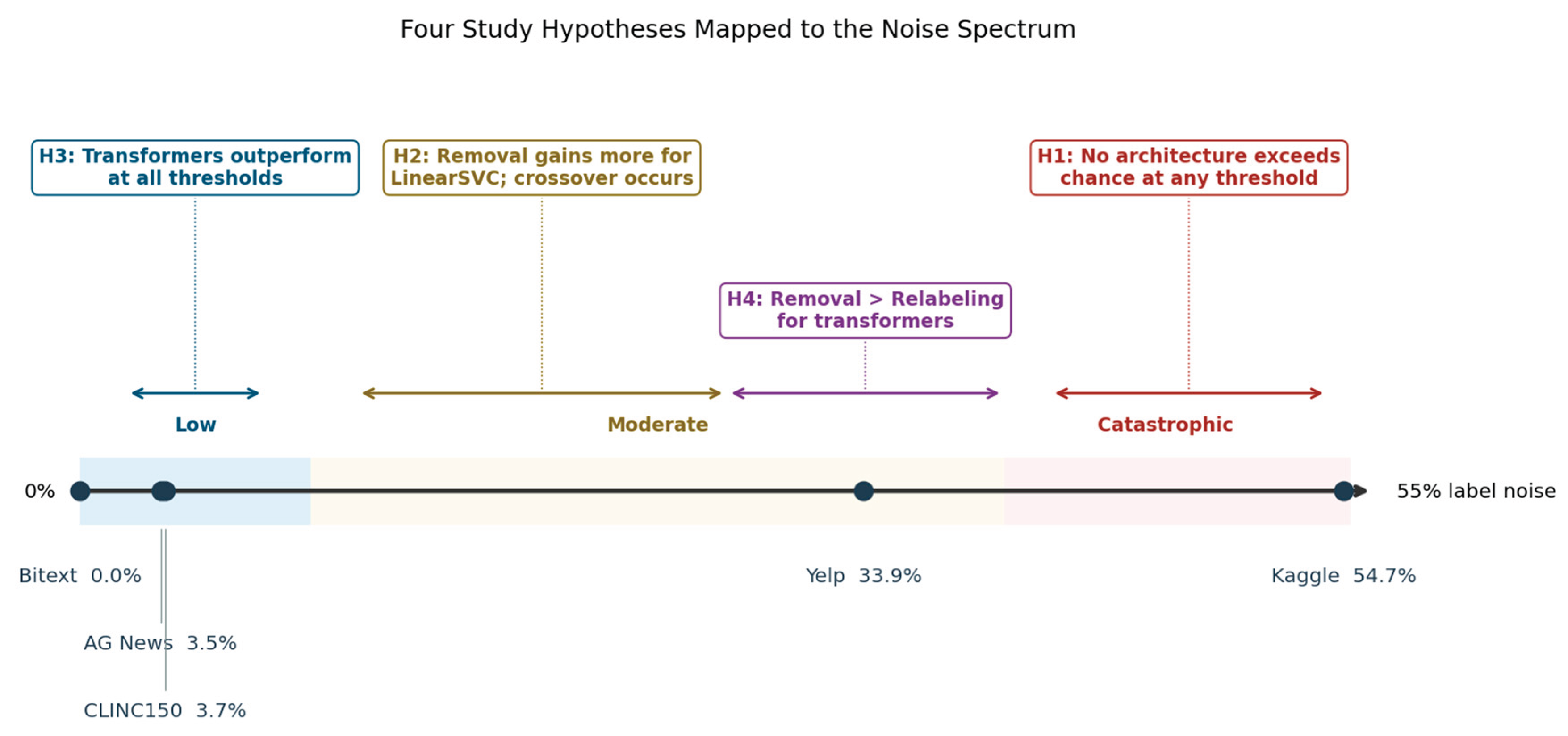
Figure 5.
All four study hypotheses located within a noise-regime by architecture-type grid. Note. H1 governs Zone III; H3 governs Zone I; H2 and H4 both operate within Zone II, with H4 addressing strategy-level differences within that regime.
Figure 5.
All four study hypotheses located within a noise-regime by architecture-type grid. Note. H1 governs Zone III; H3 governs Zone I; H2 and H4 both operate within Zone II, with H4 addressing strategy-level differences within that regime.
Each hypothesis will be addressed by specific evidence in the Results Section, and the integrated interpretation will be developed in the Analysis and Interpretation (Discussion) Section.
Contributions and Study Narrative
This study’s contributions address four questions that a reader is likely to ask about when reviewing the study design. First, is the detection methodology reliable enough to trust the downstream results? The independent validation of the confident learning detection pipeline against the CIFAR-N ground truth corpus of Wei et al. (2022) provided a foundation for understanding how reliable the method will be when applied in practice (i.e., established a reliability “floor”). This validated approximately a 25% detection reliability for uniformly random errors and 20% detection reliability for class-conditional errors. This validated methodology is reported separately from the downstream classification results as the validity of downstream classification results depends on the reproducibility of this validated methodology.
Second, does data quality remediation actually work, and if so, under what conditions? A controlled remediation experiment was conducted with 135 different test conditions. The study used five corpora and examined the effects of noise across the range of 0.0% to 54.7% detected noise with three different families of models, also using two different remediation techniques and five different remediation thresholds. Each of the models used the same architecture so that model architecture remains constant along the range of noise levels, while the data being evaluated varies in quality across the noise gradient. The resulting performance curves for the three different types of models provided a level of detail and resolution that has not been previously provided in any of the literature reviewed for this study (Song et al. 2022).
Why does the third reason explain the way the pattern looks? The third reason is conceptualized using a theoretical model that combines the bias-variance trade-off and inductive bias (Geman, Bienenstock, and Doursat 1992; Zhang et al. 2017) to explain the structural difference between the LinearSVC and the transformer architectures. The LinearSVC has high inductive bias due to the constraints of its linear decision surface and its reliance on a fixed TF-IDF feature set to determine its decision boundary. Therefore, this type of model offers a certain level of protection against label noise. In contrast, DistilBERT and RoBERTa are low-inductive-bias models and allow for a more complex representation of knowledge, which makes them susceptible to encoding noise within the label system. This perspective on the relationship between the bias-variance trade-off and inductive bias provides a framework for understanding three empirical observations: (1) LinearSVC maintains greater resiliency under high noise conditions than transformers, (2) LinearSVC loses superiority as the amount of noise is decreased, and (3) all models collapse uniformly under catastrophic levels of noise. Other theoretical views including effective sample size and information theory will be discussed in the Analysis and Interpretation Sections.
Fourth, how much does this cost in practice? Cost-performance Pareto frontiers were generated across four annotation cost tiers spanning the landscape of 2025 to 2026: (1) LLM-assisted annotation (Ratul et al. 2026), (2) crowdsourcing (Gilardi, Alizadeh, and Kubli 2023; Aguda et al. 2024), (3) professional annotators (Kang, Xu, and Ritter 2023; Donhauser et al. 2026), and (4) expert human review (DataX Power 2026). The wide range of costs, spanning four orders of magnitude, illustrates the separation of the economics of annotations identified by Carlson and Burbano (2026) as a transformation of the way in which the costs of performing data-related operations are considered.
This report is organized into seven sections and four appendices: Literature Review, Data, Methods, Results, Analysis and Interpretation, Conclusions, and Directions for Future Work. The Literature Review locates the research in the literature on labels, data-centric AI, bias-variance tradeoff and inductive bias, cost-performance analysis, and concludes with a theoretical framework for understanding architecture-noise interactions through the lens of inductive bias in classifying the architectures compared in this study. The Data Section provides information on the selected and preprocessed corpus, while the Methods Section provides information on experimental design, confident learning detection pipeline, remediation strategies, model architectures, statistical framework, and cost-performance analysis framework. The Results Section includes CIFAR-N validation results, performance-quality curve for all five corpora, architecture divergence analysis, and composition of the Pareto frontier. The Analysis and Interpretation Section will connect empirical results to the theoretical framework, discuss alternative theoretical interpretations of the results, and develop practitioner-actionable conclusions using a decision-making framework. Conclusions and Directions for Future Work are the two last sections included in the report, with a total of four appendices. The appendices will include full results at a total of 135 conditions, full pairwise significance tables, noise characterization figures specific to each corpus, and pilot study design data per corpus.
Literature Review

Table 1.
Literature streams reviewed, key gaps, and this study’s contributions.
| Literature Stream | Key Gap Identified | This Study’s Contribution |
|---|---|---|
| Label noise in supervised classification | Point comparisons at fixed noise levels; no continuous gradient across noise regimes (Song et al. 2022) | 135 conditions across a 0.0–54.7% noise gradient with per-corpus performance-quality curves |
| Data-centric AI | Evidence skewed to computer vision; NLP-specific validation absent (Sambasivan et al. 2021) | Controlled NLP remediation experiment holding architecture constant across the noise gradient |
| Architecture comparisons in NLP | Transformer vs. shallow baseline comparisons under label noise not characterized (Zhu et al. 2022) | Three architectures evaluated under systematic remediation: LinearSVC, DistilBERT, RoBERTa |
| Bias-variance tradeoff and inductive bias | No characterization of how inductive bias determines architecture resilience to label noise | High-bias (LinearSVC) vs. low-bias (DistilBERT, RoBERTa) distinction applied to interpret architecture-noise interactions |
| Cost-performance analysis in ML | No Pareto frontier analysis of data quality vs. architectural investment in text classification | Cost-performance frontiers at four annotation-cost tiers spanning the 2025–2026 landscape |
Note. Each row corresponds to one subsection of the Literature Review that follows. The “Contribution” column previews the corresponding empirical or theoretical element described in the Contributions and Study Narrative subsection of the Introduction.
Label Noise in Supervised Classification
Frénay and Verleysen (2014) first established the theoretical model for labeling errors in supervised classification by describing three types of labeling error mechanisms, which have influenced subsequent research. These mechanisms are random, conditional random, and non-random labeling mechanisms. Random labeling errors occur irrespective of the feature values and true class. They would affect all instances equally, regardless of their respective feature vectors and labels. Conditional random labeling errors only affect instances according to their true class. Non-random labeling errors occur only based upon the feature vector of a given instance. Song et al. (2022) extended the conceptual constructs of Frénay and Verleysen (2014) to include an extensive review of deep learning methods for labeling error correction, distinguishing between loss correction, sample selection, and regularization. Despite having presented an empirical comparison between labeled and unlabeled data within a supervised context, Song et al. (2022) focused primarily on direct comparison between labeled training data and unlabeled training data, rather than controlling for varying levels of labeling error across a continuum. This provided an avenue for future research.
Northcutt, Jiang, and Chuang (2021) created a statistical method called “probabilistic label error detection,” which estimates the degree of error in the training labels for supervised learning models. This method compares the probabilities produced by a model to the training labels provided and flags instances where the model’s confidence in the predicted label differs from the label given. The method builds a joint probability distribution for noisy and true labels by calculating the out-of-sample prediction probabilities, and has been made available as the cleanlab open-source library. Although this method has gained significant use and export popularity, there have been limited independent studies validating the performance of this methodology at high levels of noise. The CIFAR-N benchmark dataset was created by Wei et al. (2022) to provide a validated set of images for CIFAR-10 and CIFAR-100, which include human annotated images at an established concentration of noise, allowing for independent validation of the reliabilities of the cleanlab methodology to detect label errors using the CIFAR-N data. At the time of writing of this report, no independent validation studies were found for cleanlab’s methodology within the NLP setting using CIFAR-N data.
Data-Centric Artificial Intelligence
Ng (2021) outlined how to structure a data-centric artificial intelligence paradigm. The data-centric approach looks at how to optimize data quality rather than optimizing models in a traditional pipeline. Zha et al. (2023) created a taxonomy that collects data-centric methods under three common categories, which are training data development, inference data development, and data maintenance. Whang et al. (2023) created a complementary taxonomy that focused on data collection and quality issues for production machine learning (ML) systems. Renggli et al. (2021) gave empirical evidence for data-centric methods on a subset of benchmark datasets. Jain et al. (2020) provided a survey of the systems needed to enable a data-centric approach to operation on very large scales.
The core data-centric claim has been supported with empirical evidence but the amount of evidence differs by domain. The most compelling findings are in computer vision. In computer vision, controlled studies demonstrate that, for certain benchmark tasks, targeted investments in data quality resulted in greater improvements in task performance compared to improvements in model design (Sambasivan et al. 2021). For NLP, the evidence is less consistent. A study by Aroyo and Welty (2015) illustrated that annotation errors related to disagreement within NLP corpora appear to occur systematically, which contradicts the assumption that label errors can simply be viewed as random noise to be filtered out. Klie, Eckart de Castilho, and Gurevych (2024) illustrated that artifacts created by human annotators in text classification differ significantly depending on the particular task being performed. Consequently, findings from one corpus cannot be generalized to other corpora. Therefore, the data-centric claim needs to be empirically validated within the domain of interest. This study conducts such an empirical validation for text classification.
Architecture Comparisons in NLP Classification
Vaswani et al.’s (2017) paper introduced the transformer architecture that is responsible for most of today’s highest scoring NLP models, which was further developed to allow for bidirectional pretraining with Devlin et al. (2019). Rogers, Kovaleva, and Rumshisky (2020) gave a detailed overview of what is learned during BERT-style model pretraining, and how that information is passed onto the downstream task. DistilBERT (Sanh et al. 2019) and RoBERTa (Liu et al. 2019) are two variations of the base BERT architecture, in that they represent different options for balance between computational cost and amount of represented knowledge, respectively. Zangari et al. (2023) analyzed the use of such models for the purposes of intent classification and automated ticketing. The authors found that transformer models provide significantly improved performance when compared with increasingly shallow baseline models, especially in similar types of fine-grained multi-class classification tasks.
The existing body of literature has not characterized how transformer architectures compare to shallow baselines when both face label noise. Zhu et al. (2022) highlighted how transformer architectures have the ability to learn or memorize label noise while being trained through fine-tuning; however, their experimental comparisons were limited to the use of other transformer architectures. Xie et al. (2020) found that using self-training with label noise could provide benefits to transformer architecture accuracy under specific circumstances and conditions. However, neither study compared against shallow baselines. The architecture crossover phenomenon observed in this study, where the accuracy of a shallow baseline overtakes that of a fine-tuned transformer when the quality of training data improves, has not been described in the literature reviewed.
Bias-Variance Tradeoff and Inductive Bias
The classical bias-variance tradeoff provides a theoretical framework to understand how different model architectures behave under label noise. The classical theoretical decomposition of expected prediction error into a bias term representing structural constraints imposed on the model’s hypothesis space, variance resulting from the model’s sensitivity to fluctuations in its training data, and non-recoverable label noise due to uncertainty in the labeling process, was first proposed by Geman, Bienenstock, and Doursat (1992). High-bias, low-variance models place severe restrictions on what types of information they can learn from the training data while they are robust against noise in the training signal. Conversely, low-bias, high-variance models allow them to learn more complex patterns from the training data but also have a greater propensity to mistake noise for information when they are trained.
Zhang et al. (2017) demonstrated that deep neural networks can memorize training data with random labels while generalizing on structured data. Therefore, low-bias, high-variance models have adequate capacity for encoding the corrupted structure of the label as an actual signal. This capacity is the reason that transformer architectures are prone to label noise. Self-attentive transformer models are contextually rich and can therefore encode atypical structures of labels in addition to incorrect labels (Zhu et al. 2022). LinearSVC has fewer vulnerabilities to label noise compared to transformer models since the LinearSVC’s linear decision boundary is fixed in the TF-IDF feature space, therefore limiting the model’s ability to fit arbitrary label assignments and indirectly shielding it from being affected by label noise due to this structural difference in inductive bias. The outcome of this difference in inductive bias can be represented in terms of crossover phenomena during empirical testing.
Cost-Performance Analysis in Machine Learning
The cost of annotating data has constrained supervised learning research since crowdsourced annotations were first made available via Amazon Mechanical Turk (Snow et al. 2008). Kang, Xu, and Ritter (2023) documented per-instance annotation costs of $0.26 to $0.44, providing one of the few peer-reviewed cost benchmarks for text annotation. However, it was reported by Gilardi, Alizadeh, and Kubli (2023) in Proceedings of the National Academy of Sciences that LLMs can achieve performance matching or exceeding that of crowdworkers at approximately 1/30 of the cost of crowdworkers, on text annotation tasks. This research has been confirmed and extended to include LLMs for annotating financial data (Aguda et al. 2024), LLMs to classify citations (Ratul et al. 2026), and LLMs for classifying the sentiment of aspects (Donhauser et al. 2026). All of these studies showed an order of magnitude in the cost savings when using annotation via LLMs instead of crowdworker annotation. It was established by Carlson and Burbano (2026) in the Strategic Management Journal that LLMs will come to dominate research methodology choices that were previously determined solely by the cost of annotation.
The AutoML literature published a definition of the Pareto frontier framework to evaluate cost-performance trade-offs within machine learning (He, Zhao, and Chu 2021). For example, in their paper Schwartz et al. (2020) demonstrated how this framework could be applied to model selection given compute constraints. However, the Pareto framework has not been applied in prior text-classification work to evaluate trade-offs between data-quality and architecture investments, which is the gap this study addresses. As such, the purpose of this present study is to demonstrate an extension of the application of the Pareto framework for evaluating these respective investment opportunities by mapping out the 2025–2026 cost landscape for all annotations (at a cost spanning across four orders of magnitude of annotation costs).
Theoretical Framing
This study looked at how the bias-variance tradeoff can help explain how architecture and noise interact within supervised classification models. In supervised classification, the expected prediction error of a model can be split into three components: (1) bias, which comes from the structural assumptions made by the model when creating a hypothesis space, (2) variance, which results from the model’s sensitivity to fluctuations across different training samples, and (3) non-recoverable label noise, which is due to the fact that there will always be some uncertainty involved in the labeling process (Geman, Bienenstock, and Doursat 1992). A model that has high bias but low variance places strong constraints on what it can learn but would be more robust against the noise in the training data. Conversely, a model that has low bias but high variance has the potential to fit very complex patterns, but would be more likely to misinterpret the noise in the data as meaningful signals.
LinearSVC models are categorized as high-bias, low-variance models when viewed through the lens of the framework described above. As LinearSVC works structurally with the linear nature of a single hyperplane decision boundary, the structural limitation of such a model eliminates the potential for creating arbitrary latent dimensions based upon various combinations of feature vectors (or TF-IDF vectors). Because of this inherent structural limitation, there is limited potential to create a structure that can remember incorrectly labeled examples (due to the inability to create multiple representations). Conversely, a deep learning model (such as DistilBERT or RoBERTa) contains enough representational flexibility to create representations that will allow the model to maintain the structural representation of its training data (even if it includes incorrect labels). This allows the model to perform exceptionally on clean datasets but also indicates that these types of models will be less robust to the effects of label noise.
The first three hypotheses presented in the introduction predict the following three things: (H1) that when the label noise is so extreme that there is no relationship left between the input feature set and label set that can be recovered from either architecture, both architectures will fail equally and that this failure will serve as an indicator for irretrievable data corruption rather than correctable errors, (H2) that as remediation reduces data corruption, the transformers will regain their competitive advantages because of the way they represent data, thus creating an architecture crossover, and (H3) that LinearSVC will experience less influence from corrupted data due to noise compared to transformers when trained on a dataset with the most substantial noise. In the section labeled Analysis and Interpretation, there will also be discussion regarding alternative theoretical explanations for the patterns observed in the study.
Data
Corpus Selection Rationale
Five different text classification datasets were sampled to create a label noise gradient from clean through catastrophic. For each of the three regimes (low, moderate, catastrophic), datasets were sampled to represent that noise level. Two datasets from a pilot study performed by Senne (2026) were included to provide continuity with previously established baseline macro F1 scores for LinearSVC and DistilBERT, as well as the opportunity to generalize beyond the pilot study. In total, the datasets sampled for this project allowed for an effective assessment of the validity of the data-centric argument and provided reasonable baseline macro F1 scores for both LinearSVC and DistilBERT under five-fold stratified cross-validation. The factorial analyses conducted across all sampled datasets necessitated Bonferroni adjustments to the significance tests.
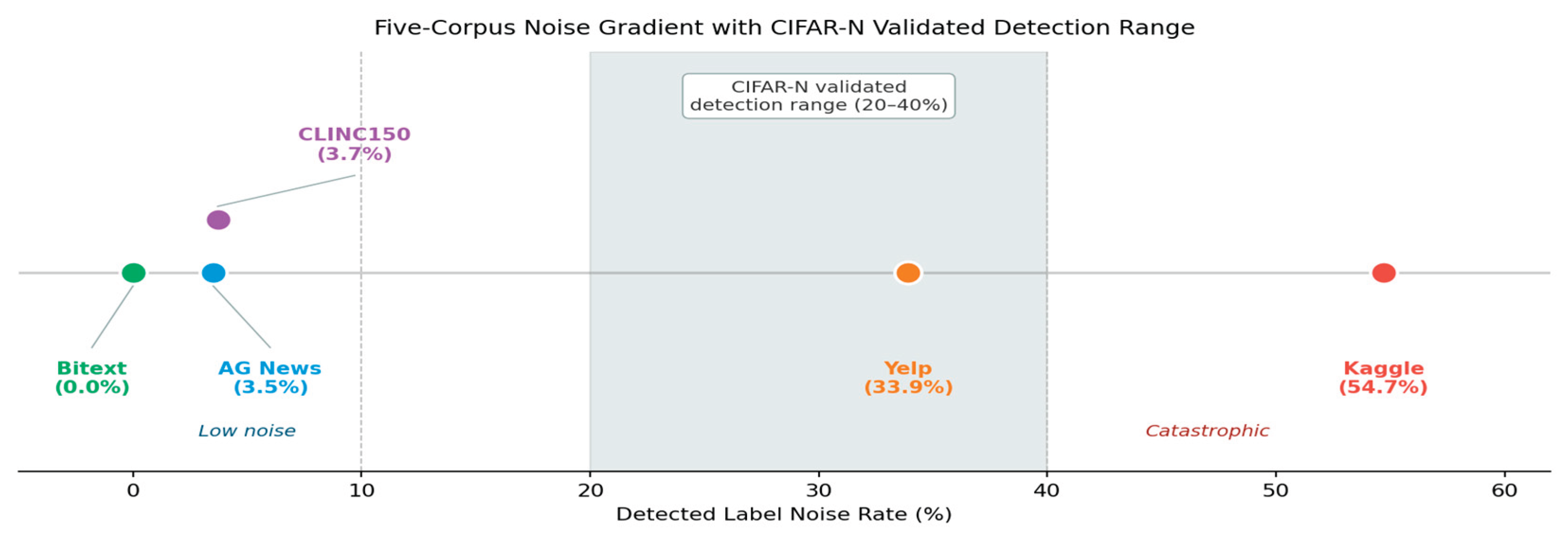
The Bitext support corpus (Bitext Innovations 2023) consists of 26,872 utterances and contains 27 different intents, providing a solid baseline level for determining levels of noise. The confident learning algorithm found only 5 potential label errors for the Bitext support corpus, yielding an overall rounded noise rate of 0.0%. The CLINC150 Intent Classification Corpus (Larson et al. 2019) has 22,500 utterances classified into 150 intents and has a noise rate of 3.7%. The synthetic Kaggle Support Customer Service Corpus (Suraj 2023) contains 8469 tickets created through synthetic methods and has a noise rate of 54.7%. The AG News Corpus (Zhang, Zhao, and LeCun 2015) consists of professionally edited articles from news sources, with a noise rate of 3.5%. The Yelp Review Full Corpus (Zhang, Zhao, and LeCun 2015) contains customer reviews that were rated from 1–5 stars and is a good example of noise related to sentiment labeling. The overall rounded noise rate for the Yelp Review Full Corpus is 33.9%. A summary of the contents of each corpus is in Table 2.
These five corpora form a gradient over approximately 55 percent of noise detected. This level of detail could not be achieved with point-in-time comparisons of fixed levels of noise in previous studies of detected noise via point-in-time (Song et al. 2022). As such, including the Yelp Review Full corpus was necessary, as it provides organic label (star) noise created by the inherent ambiguity of star ratings as sentiment proxies. Whereas, most of the label noise in the literature has been artificially created using injections (Song et al. 2022).
Table 3.
Corpus noise gradient relative to the CIFAR-N validation range.
| Corpus | Detected Noise Rate | Within Validated Range (20–40%)? | Regime |
|---|---|---|---|
| Bitext | 0.0% | Below floor | Clean baseline |
| AG News | 3.5% | Below floor | Low, professional text |
| CLINC150 | 3.7% | Below floor | Low, fine-grained intent |
| Yelp Review Full | 33.9% | Yes | Moderate, natural noise |
| Kaggle Customer Support | 54.7% | Extrapolation required | Catastrophic, synthetic |
Note. The validated range (20% through 40%) is set by the CIFAR-N detection reliability validation as explained in the Methods Section, which means that any corpora that fall below 20% will be below the detection reliability floor. Therefore, at those noise rates, the results will indicate label cleanup only rather than substantive noise correction. The Kaggle corpus is 54.7% so is outside the validated range; thus, any analyses done on this corpus will contain some level of uncertainty because the detection reliability at that noise rate has not been directly validated.
Figure 6.
Five-corpus noise gradient from 0.0% to 54.7% detected label noise. Note. Shaded band = CIFAR-N validated reliable detection range (20–40%). Corpora below the band fall below the detection reliability floor; Kaggle (54.7%) exceeds it and is interpreted with corresponding uncertainty.
Figure 6.
Five-corpus noise gradient from 0.0% to 54.7% detected label noise. Note. Shaded band = CIFAR-N validated reliable detection range (20–40%). Corpora below the band fall below the detection reliability floor; Kaggle (54.7%) exceeds it and is interpreted with corresponding uncertainty.
Preprocessing Pipeline
The preprocessing pipeline for all corpora follows the same process to make it possible to compare results across the gradient of noise present. This pipeline has been developed as part of a previous pilot study and is made up of five steps (Senne 2026). The content is changed to lower case, and any HTML tags, URLs, email addresses and placeholder tokens (like Bitext-style tokens) are removed using regular expressions. Tokenizing the text occurs with the spaCy library (3.8). Stopwords from the English-language to be used with NLTK have been eliminated. Lemmatization was done using the spaCy lemmatizer, but the named entity recognition and dependency parsing will not be activated for efficiency in compute time requirements. The final output from this pipeline has two fields, a text_clean for input into the TF-IDF feature extraction and a text_lemma for use with any architectures that require lemmatized input.
For the transformer architectures, models were trained on raw input (i.e., the text before the initial clean up), and have kept the same morphological tokenization method used to train them as well as preventing artifacts generated by preprocessing from influencing fine-tuning. In contrast, many other NLP models, such as TF-IDF models, are built on a lemmatization of raw input (i.e., all words are converted back to their original form) (Rogers, Kovaleva, and Rumshisky 2020).
Data and Code Availability
The data sets used in this research are listed in Table 2. All data and analysis, including data preprocessing scripts (i.e., output from phases 1–4 including macro F1 scores for each condition and fold), bootstrapping code, remediation plan codes based on confident learning, model fine-tuning and cost performance plots, and pilot study notebook, are available as open source at https://github.com/joshuasenne2027-lab/data-quality-vs-architecture-nlp. The output files from phases 1–4 can be found in the results/ directory of the repository. To replicate this work, access to a CUDA-capable GPU is needed (the study was conducted using the NVIDIA A100 40GB), along with 15 to 20 h of GPU processing time to complete all full RoBERTa conditions and the software dependencies found in the requirements.txt file in the repository.
Methods
Experimental Design
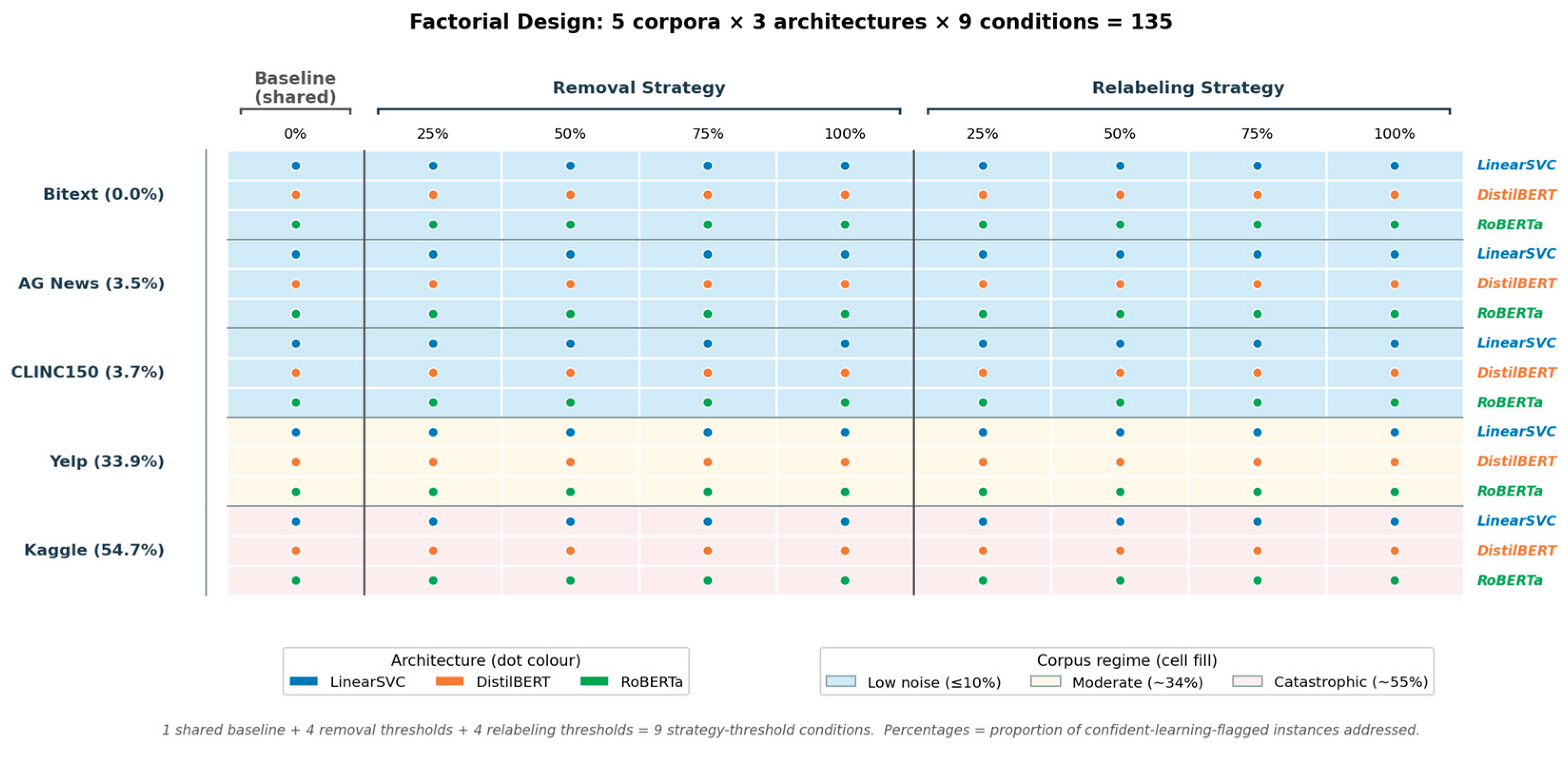
The experimental design uses a full factorial approach, with three factors (i.e., corpus (5 levels), model architecture (3 levels), and remediation strategy at threshold (9 levels)) being manipulated. The five corpora are described in the Data Section. The three model architectures are as follows: LinearSVC (as a shallow bag-of-features baseline), DistilBERT (as a compressed transformer), and RoBERTa (as a full-scale transformer). The nine-remediation strategy-threshold combinations consist of removal at 0%, 25%, 50%, 75%, and 100% of detected issues addressed and relabeling at 25%, 50%, 75%, and 100% of detected issues addressed. The 0% relabeling condition is not included, as it is definitionally the same as the 0% removal condition. The complete factorial produces a total of 5 × 3 × 9 = 135 experimental conditions.
Five-fold stratified cross-validation was performed on the remediated corpus for each of the conditions. Stratifying the folds allows for the preservation of class balance between folds, which is critical when working with the imbalanced Kaggle corpus and the CLINC150 corpus (which has 150 classes). All performance metrics were calculated using a macro-averaged F1 score, which gives equal weight to all classes, regardless of their respective frequencies. In addition, standard deviation across folds was used to characterize the stability of each condition. All conditions used random seed number 42 so they can be reproduced.
Table 4.
Factorial design structure producing 135 experimental conditions.
| Factor | Levels (N) | Values |
|---|---|---|
| Corpus | 5 | Bitext, AG News, CLINC150, Yelp Review Full, Kaggle Customer Support |
| Model architecture | 3 | LinearSVC (TF-IDF), DistilBERT (distilbert-base-uncased), RoBERTa (roberta-base) |
| Remediation strategy × threshold | 9 | Removal: 0%, 25%, 50%, 75%, 100%; Relabeling: 25%, 50%, 75%, 100% |
| Total conditions | 135 | 5 × 3 × 9 = 135; each evaluated by 5-fold stratified cross-validation (seed 42) |
Note. The 0% relabeling condition was excluded because it was defined as being exactly the same as the 0% removal condition, resulting in nine (vs. ten) strategy/threshold combinations for each architecture/corpus pair. The total number of conditions (135) means that there are five macro F1 scores (one per fold) computed for each condition, and the overall mean and standard deviation across all of these five values have been calculated.
Figure 7.
Factorial design: 135 experimental conditions (5 corpora × 3 architectures × 9 strategy-threshold combinations). Note. Color indicates corpus noise regime. R = removal; L = relabeling. Threshold values indicate the proportion of flagged instances addressed.
Figure 7.
Factorial design: 135 experimental conditions (5 corpora × 3 architectures × 9 strategy-threshold combinations). Note. Color indicates corpus noise regime. R = removal; L = relabeling. Threshold values indicate the proportion of flagged instances addressed.
Confident Learning Detection Pipeline
Confident learning was used to identify potential label errors in each of the five corpora before remediation. The pipeline consists of three stages. The first stage is a TF-IDF pipeline with a calibrated LinearSVC classifier that uses five-fold cross-validation to create out-of-sample predicted probabilities. The calibrated LinearSVC was chosen as the base estimator because it provides a probabilistic output and works well with all five corpora. In the second stage, the cleanlab find_label_issues function is used to identify all instances for which the assigned label and confident prediction do not agree according to the joint distribution estimation procedure outlined by Northcutt, Jiang, and Chuang (2021). In the final stage, the instances flagged by the cleanlab find_label_issues function are ranked based on self-confidence, which is defined as the probability assigned to the given label by the model. This ranking allows for the most confidently mislabeled instances to be addressed first during remediation.
Detection compute has been factored into the overall analysis of the Pareto frontier as a sunk cost because it is incurred once per corpus regardless of the downstream remediation strategy. The time required for detection was, on average, 0.170 s of cleanlab processing per corpus after generating the out-of-sample probability, and from 4 to 6 s of processing time for each corpus in total to do the out-of-sample probability generation. Thus, this detection expense will be trivial if compared to both the transformer fine-tuning compute costs and re-labeling annotation expenses.
CIFAR-N Detection Reliability Validation
The CIFAR-N dataset was used to independently validate the confident learning pipeline before applying it to the five text classification corpora. The CIFAR-N dataset provided a direct sample of what the label errors would be, allowing the user to calculate the true positive, true negative, precision, recall, and F1 for every detection. The CIFAR-10 dataset was used to create 12 separate validation conditions by injecting synthetic noise at rates of 10%, 15%, 20%, 25%, 30%, and 40%, by both random uniform and class conditional errors. All detection metrics were calculated for each condition based on the CIFAR-N validation dataset.
This validation acts as a prerequisite for the downstream classification experiments. Each noise type has been assigned a threshold regarding the detection F1 score of 0.20 based upon studies reported in the current literature related to the concept of confident learning (Northcutt, Jiang, and Chuang 2021). An F1 score over this threshold means that the confident learning process and pipeline used in the creation of this dataset will perform accurately enough to proceed with downstream remediation, whereas an F1 score below this threshold suggests that any measure of success resulting from remediation will be due to chance or incidental training set reduction, and not actual correction of noise. The contribution and methodological novelty here are reported separately from the downstream classification results obtained by conducting this experiment.
Remediation Strategies
Both remediation strategies were implemented at each of the five thresholds. The removal strategy consists of removing flagged instances from the training corpus according to their self-confidence level, with the most confidently mislabeled instances being removed first. The relabeling strategy consists of changing the label for each flagged instance using the label suggestion algorithm from cleanlab (i.e., the label with the highest probability as determined by a model under a joint distribution estimation). The five thresholds are designed to address 0%, 25%, 50%, 75% and 100% of the flagged instances, respectively. The resulting gradient of remediation intensity allows for the production of performance-quality curves.
By comparing the two methods of intervention (relabeling and removing), practitioners can see clearly which method will work best for them as not all practitioners will be able to afford to have a human annotator look at all of their suggested labels. Removal is automatic after detection and requires no additional human resources. Relabeling, however, does require either reviewing the recommended label by a human annotator or accepting the suggested label by the ML model without any human input. Each of these two approaches therefore has costs associated with it, and comparing them isolates the monetary value of the label information for the flagged instances from the monetary benefit of removing the noisy instances from the training data.
Model Architectures and Training
The previous pilot study (Senne 2026) specified the following configurations for the three model architectures: LinearSVC and DistilBERT, which were included in order to assess whether the architecture crossover phenomenon can be extrapolated to other types of models (i.e., transformer models), as RoBERTa was included as an additional test. The training of LinearSVC was done with a class-balanced loss function and included TF-IDF features with a maximum of 20,000 features, and bigram n-grams with a minimum document frequency of 2. The C parameter for LinearSVC was tuned for each dataset during the pilot study. DistilBERT was fine-tuned from the DistilBERT checkpoint (Sanh et al. 2019) for 4 epochs using a maximum sequence length of 128 tokens, with a batch size of 16 and a learning rate of 2 × 10⁻⁵. RoBERTa was also fine-tuned using the same parameters, as noted in Liu et al. (2019), as DistilBERT, except for the actual model architecture. All transformer fine-tuning was performed on NVIDIA A100 GPUs with FP16 mixed precision for shorter compute times.
Statistical Analysis Framework
To test for significance between architectures, pairwise t-tests were performed on the five-fold macro F1 scores as recommended in Dietterich’s (1998) work comparing supervised classification algorithms across the same folds. The number of comparisons made in this experiment (150 total pairs) forced the use of statistical adjustment via Bonferroni’s method, therefore, the corrected alpha level was 0.000333 (0.05/150). The effect sizes were determined by calculating Cohen’s d from the paired fold-level F1 differences. The mean F1 of each condition’s bootstrapped 95% confidence interval was calculated using 10,000 total resamples of the five-fold F1 scores.
Cost-Performance Analysis Framework
To obtain cost-performance Pareto frontiers, two components of the costs were combined into a composite cost axis for each corpus. The first is the compute costs for cross-validation training derived from the wall-clock time to cross validate that was measured and then converted to GPU hours computed with an hourly rate. The reference for the on-demand rate is Google Cloud Platform a2-highgpu-1g at $3.67/hour for one NVIDIA A100 40GB GPU (Google Cloud 2026). This rate is midpoint between Lambda Labs (which charged $1.99/A100 h) and Databricks Mosaic Training (charged $4.75/A100 h). As a result, it is a representative on-demand price for practitioners who do not have a committed use discount on their cloud services.
Annotation costs apply only to relabeling strategies, as there is no additional marginal annotation cost associated with removing an instance after its detection. Annotation costs associated with relabeling are calculated using the number of remediated instances times the per-instance annotation cost. Four different annotation rate tiers were established to represent the environment of annotation costs for 2025–2026. The LLM economical tier is $0.0003 per instance. This corresponds to the documented “flash” annotation cost by Gemini 2.5 (Ratul et al. 2026) and serves only as an illustration of LLM pricing, which has rapidly changed and is based on one citation only. The crowdworker baseline tier is $0.10 per instance and is the same as the crowdworker baseline described in Aguda et al. (2024) and Gilardi, Alizadeh, and Kubli (2023). The tier of professional crowdworkers, which is $0.40 per instance, is based on Kang, Xu, and Ritter (2023) and Donhauser et al. (2026) regarding stance classification and aspect-based sentiment analysis. The expert human tier (within the cost range of $1–5) is $2.00 per instance as noted by DataX Power (2026).
If there is a combination of a corpus and annotation rate that is Pareto-optimal, that means no other combination of corpus and annotation rate has both a higher F1 score and a lower or equal total cost. The set of all Pareto-optimal conditions is known as the Pareto frontier. For both the sensitivity of the composition of the Pareto frontiers and the sensitivity of the annotation rates, a detailed analysis was conducted.
Table 5.
Annotation cost tiers used in the Pareto frontier analysis.
| Tier | Rate per Instance | Representative Modality | Source |
|---|---|---|---|
| LLM economical | $0.0003 | LLM batch annotation (Gemini 2.5 Flash) | Ratul et al. (2026) |
| LLM frontier/crowd floor | $0.10 | LLM frontier or crowdworker baseline | Aguda et al. (2024); Gilardi et al. (2023) |
| Professional crowdworker | $0.40 | Stance classification; ABSA crowdworker rate | Kang, Xu, and Ritter (2023); Donhauser et al. (2026) |
| Expert human | $2.00 | Midpoint of $1–$5 expert-required annotation range | DataX Power (2026) |
Note. The aforementioned four-order-of-magnitude range across tiers represents the bifurcation of annotation economics as described in the Carlson and Burbano (2026) study. The LLM economical tier is meant only to illustrate the range of LLM pricing rather than to be definitive, as LLM pricing is still evolving at a rapid pace. The annotation cost is applicable only to the relabeling strategy, while removal incurs no marginal annotation cost after the removal has been detected.
Results
CIFAR-N Detection Reliability Validation
The confident learning pipeline, which utilizes the detection metrics of precision, recall, and F1 score for detection, was evaluated across all 12 CIFAR-N validation conditions including 2 noise types and 6 injection rates. The complete evaluation results are shown in Figure 8. F1 scores for detection increase monotonically as noise rates increase for both noise types, indicating that as the corruption rate increases, so does the availability of an increased signal to the detection algorithm. For all injection rates tested, uniform random noise was detected at a higher reliability than class-conditional noise. Using a 25% noise rate as a benchmark for reliable detection that has been used in previous works on confident learning (Northcutt, Jiang, and Chuang 2021), the F1 scores for detection were 0.516 for uniform noise and 0.426 for class-conditional noise. At a 40% noise rate, which is above the majority of natural noise levels found, the F1 scores for uniform noise and class-conditional noise were 0.605 and 0.482 respectively.
The findings establish a reliability floor for the confident learning pipeline that qualifies the interpretation of downstream classification findings. For Bitext and CLINC150 low-noise datasets, with detected noise rates of 0.0% and 3.7%, respectively, these noise rates are lower than what would indicate reliable CIFAR-N validation for the detection system and remediation findings should be seen as reflecting minor label cleanup rather than substantive noise reduction. This also applies to AG News, which had a detected noise rate of 3.5%. However, for Yelp, the detected noise rate (33.9%) is within the CIFAR-N validated range, and the projected detection F1 score by linear interpolation is 0.568 for uniform noise and 0.465 for class-conditional noise. For Kaggle, a detected noise rate of 54.7% falls above the validated range therefore the projected detection F1 score must be extrapolated. Given this lack of direct validation of detection reliability at this level of noise, Kaggle findings must be treated with substantial uncertainty.
Corpus-Level Noise Detection
Noise detection results of all 5 corpora are presented in Table 6. The range or gradient of noise detection rates was 0.0% for the Bitext corpus to 54.7% for the Kaggle corpus, which provided the experimental design with the full noise gradient required. Appendix C contains details about each corpus, including the rate of noise per class, a graph representing all self-confidence levels from each class, and the label transition heatmaps.
Performance-Quality Curves Across Corpora
The performance-quality curves shown in Figure 9 are presented for all 5 corpora based on each remediation strategy (i.e., the removal strategy versus the relabeling strategy). Each of the 5 rows represents the 5 different corpora arranged with respect to increasing levels of detected noise. The 2 columns differentiate between the 2 remediation strategies, i.e., the removal and relabeling remediation strategies.
The curves demonstrate consistency in their patterns based on the noise level of the corpus (i.e., Bitext). In every single case, all three of the models achieved a macro F1 greater than 0.99, and remediation had no discernible effect. The clean baseline represents the highest possible score for this metric and can’t be further enhanced. For the other dataset (CLINC150), all transformer architectures substantially outperform LinearSVC at all thresholds. RoBERTa achieves its highest performance at 0.9821, DistilBERT reaches 0.9711, and LinearSVC achieves 0.9207. Moreover, when noise is removed from these datasets, the performance of all three architectures improves monotonically. The relabeling process, however, produces monotonic decline in the performance of DistilBERT and RoBERTa on the CLINC150 dataset, which is discussed further in the Analysis and Interpretation Section.
Remediation to AG News results in adding approximately 2–3% to all three architectures. The removal method generates a slightly greater impact than the relabel method for both transformer architectures. For Yelp, the results are larger and differ depending on which type of architecture is being analyzed. LinearSVC’s baseline score increases from 0.5441 to 0.8033 in macro F1 after all of the label data has been removed, a total increase of about 26%. DistilBERT’s score goes from 0.6019 to 0.7144 using the same method, an increase of approximately 11%. Similarly, RoBERTa’s score increases from 0.6312 to 0.7458 for an increase of approximately 11%. Even though both transformer architectures began with higher baselines than LinearSVC, they continue to see substantially lower gains in the same manner. Additionally, at the removal threshold of 100%, LinearSVC surpasses both transformer architectures with respect to absolute macro F1 scores.
The listed architectures on Kaggle cannot exceed a macro F1 of 0.28 in any scenario. In comparison, LinearSVC has improved by 8 percentage points from its baseline score of 0.2018 to 0.2811 (100% relabeled). DistilBERT has a peak performance of 0.2023 for 100% relabeled data—a 3 percentage point improvement over its baseline (0.1711). RoBERTa’s maximum F1 score is 0.1976 (100% relabeled data), and across all conditions, this architecture scored lower than its expected chance level in a five-class problem. The fact that no architecture, nor either strategy has been able to score higher than chance levels, is consistent with interpreting the Kaggle data as containing non-recoverable label noise rather than being the result of label corruption that could be removed.
Architecture Divergence and Statistical Significance
Pairwise significance testing across all 150 comparisons produced a Bonferroni-corrected alpha of 0.000333. Figure 10 presents the fraction of Bonferroni-significant pairwise comparisons broken down by corpus and by architecture pair.
The divergence of the heatmap presents three different patterns of generalities. With CLINC150 having a very high difference (100% of comparisons) between LinearSVC and the two transformer architectures and only 20% difference between DistilBERT and RoBERTa, it is clear that architectural capacity has a significant impact on the fine-grained multi-class intent classification task. Between transformer variants, the specific architecture does not play nearly as much of a role. On both Bitext and AG News (which are both examples of very clean corpora), the transformer models are nearly indistinguishable from each other (0% and 30% divergence respectively); however, both differ meaningfully with respect to LinearSVC. On Kaggle, both DistilBERT and RoBERTa are indistinguishable (0% divergence) due to sharing the same failure mode, and again, LinearSVC differs meaningfully from both transformer models (30% and 60% divergence, respectively).
All three of the pairwise comparisons in Yelp show high divergence. These high divergence rates are 70% for both of the LinearSVC vs. DistilBERT and LinearSVC vs. RoBERTa pairwise comparisons, while DistilBERT vs. RoBERTa shows a smaller divergence of 50%. This corpus represents the only place where there is a statistically significant difference between the three architectures, consistent with the theoretical expectation that the most significant interactions between architectural and strategic choices would occur in moderate noise regimes. Figure 11 builds upon this knowledge by disaggregating the divergence rates by remediation threshold for each corpus and demonstrating where the significant crossovers occur.
Cost-Performance Pareto Frontiers
The per-corpus Pareto frontiers shown in Figure 12 demonstrate that there are differences in the composition of frontiers based on the various types of corpora, at the professional crowdworker annotation rate of $0.40 per instance, which corresponds to the current market rate for human annotation of multi-class text classification (Kang, Xu, and Ritter 2023; Donhauser et al. 2026). These compositional differences are directly related to those elements identified in the theoretical framework.
With regard to the three architectures on Bitext, the frontier represents the conditions of all three architectures with each of the LinearSVC removal conditions occurring at a cost of approximately $0.01 (low cost) and the DistilBERT removal conditions occurring at a cost of approximately $0.74 (medium cost), while removal conditions for RoBERTa occur at a cost of approximately $1.31 (high cost). Macro F1 values above 0.99 for all points of the frontier indicate that they represent different levels of investment in order to achieve marginal gains in macro F1 performance as opposed to whether the architecture is capable of obtaining sufficient levels of performance in the first place.
The conditions of the three architectures are presented on the CLINC150 frontier. The lowest-cost point ($0.02) occurs due to removal of LinearSVC with a threshold of 100%, this has a macro F1 score of 0.9207. The removal conditions of DistilBERT are around $0.61 to $0.62 which puts it into the mid-cost area. Removal of RoBERTa under 75% and 100% thresholds occurs around $1.04 to $1.05 with a macro F1 above 0.98. The frontier indicates that there are meaningful improvements to the F1 score through increasing the investment in architecture on this corpus, but such improvements come at a high multiple of cost.
The frontier on Kaggle has three data points, all of which are LinearSVC models. The point with the least total cost is the 100% threshold LinearSVC removal model; this model is the cheapest (approximately $0.00) and achieves a macro F1 score of 0.2048. The other two LinearSVC points are at 75% threshold and 100% threshold relabeling, which both have a higher total cost than the lowest cost point: one model is $1390, with a macro F1 score of 0.2462 while the second is $1853.60 and achieves a maximum macro F1 score of 0.2811. At no point do the DistilBERT or RoBERTa transformer models demonstrate non-dominated status under any condition, meaning that at least one LinearSVC condition offers higher F1 at lower or equal cost than any transformer condition. This is indicative of non-recoverable label noise, as when the input-output relationship cannot be recovered, the capacity of the transformer does not aid recovery.
LinearSVC removal at 100% threshold is the only frontier point on Yelp, with a total cost of $0.05 and a macro F1 of 0.8033. Every DistilBERT and RoBERTa condition is dominated by this single LinearSVC condition. On AG News, the conditions from all three architectures are represented in the frontier. Both LinearSVC conditions (removal at 50% and 100% thresholds) were located in the low-cost region (approximately $0.01), while DistilBERT (removal at 100% threshold) was located in the mid-cost region ($0.55) with a macro F1 of 0.9554 and RoBERTa (removal at 100% threshold) was located in the high-cost point ($0.96) with a macro F1 of 0.9588.
Sensitivity to Annotation Rate
The composition of the frontier is dependent upon the annotation rate assumption. Figure 13 depicts the sensitivity analysis of the four annotation rate tiers with respect to the Pareto frontiers. For example, at the LLM economical tier of $0.0003 per instance, relabeling essentially has no cost compared to compute costs, which shifts the composition of the frontier toward more favorable conditions for higher-threshold relabeling. However, for all of the professional crowdworker tier of $0.40 and higher per instance, relabeling costs dominate compute costs for high-threshold conditions (this shifts the composition of the frontier towards removal strategies).
The findings from the sensitivity analysis have direct implications for practitioners, as organizations that have already adopted LLM-assisted annotation can pursue large-scale relabeling without incurring a cost penalty. The frontier composition at that tier will be biased towards including a greater amount of remediation. However, organizations that traditionally rely on human annotations will experience growing linear cost penalties for remediating more instances and the frontier composition at those tiers will be biased towards removal. As such, an organization’s remediation strategy will depend on the annotation infrastructure they currently have in place as well as the specific corpus noise characteristics.
Analysis and Interpretation
The 135 experimental conditions produce three empirically robust findings that link to the bias-variance framework as described in the Theoretical Framing Section of this paper. Each of these three findings will be discussed in detail. Following each finding, alternative frameworks that may account for the same patterns will be offered, integrated interpretations of the three findings will be provided, and practitioner-actionable conclusions about how to act on these findings will be organized according to a decision-making framework.
Finding One: High-Bias Insulation on Catastrophically Noisy Data
The baseline F1 performance rankings show the effect of representational capacity, or lack thereof, on performance, but are not what one would normally predict from this. The model with the least representational capacity, LinearSVC, shows the best F1 at baseline while the model with the highest representational capacity, RoBERTa, shows the worst F1 at baseline. This reversal of the normal relationship between representational capacity and performance corresponds exactly to the predictions of the bias-variance framework under catastrophic levels of noise. Since the LinearSVC model is a high-bias model due to its linear decision boundary, it does not experience the absorption of noise, as it cannot embed the corrupted labeling structure within deep representations. Conversely, low-bias, high-variance models, such as RoBERTa, are capable of embedding arbitrary structure into their attention-mediated representations, so absorb the corrupted labeling signal during fine-tuning, producing output at or below chance level.
The analysis of the Pareto frontier supports the previous finding from an economic viewpoint as well. For instance, the Pareto frontier on Kaggle only has three LinearSVC points and also DistilBERT and RoBERTa do not reach Pareto-optimal status under any of the 45 conditions evaluated for each architecture. Hence, at every cost level and tier of annotation rate, at least one LinearSVC condition offers superior F1 to any DistilBERT or RoBERTa condition. From the viewpoint of a practical user, transformer capacity can offer no economic benefit when used with corpora that have this noise characteristic. The recommendation is not to invest in shallow architectures generally, which is contrary to the large body of evidence supporting the superiority of transformers on clean data, but rather to invest in shallow architectures specifically when working with corpora exhibiting catastrophic noise that no remediation strategy can adequately address.
There are two important caveats related to interpreting Kaggle’s data. First, as previously mentioned in the Results Section, the 40% noise experimental validation of detection reliability only applies to CIFAR-N datasets, while the Kaggle corpus (54.7% noise) was beyond the validated range. Therefore, a linear extrapolation assumes the same reliability of projected results (for uniform noise = 0.6054 and class-conditional noise = 0.4816). However, this linear extrapolation may overestimate the reliability of the projected results beyond the validated range. Second, while the LDA coherence score (0.566) from the pilot study establishes that the input text contains recoverable topical structure, it does not indicate whether the structure can be delineated into highly separable classification boundaries. Therefore, while the Kaggle results are consistent with non-recoverable label noise, they cannot be used to prove the presence of non-recoverable label noise in isolation. What they do demonstrate unequivocally is that there is no combination of the three architectures and the two strategies resulting in above-chance performance. The consistent failure of models to achieve above-chance performance across the parameter-complexity range serves as a diagnostic marker of this.
This research finding has direct implications for the ecological validity of the label noise literature. Most of the literature on label noise consists of studies where noise is injected through synthetic methods (Song et al. 2022), and the results from the Kaggle corpus demonstrate that synthetic noise added to a naturally structured corpus can produce failure modes that will not be improved by remediation strategies. If synthetic and organic noise produce fundamentally different failure modes, more caution needs to be taken in generalizing from the synthetic label noise literature to organic label noise conditions than what is usually taken.
Finding Two: Architecture Crossover on Moderately Noisy Data
The Yelp corpus includes the clearest empirical demonstration of the architecture crossover phenomenon, where LinearSVC achieved a macro F1 of 0.5441 at baseline and a peak of 0.8033 (100% removal), providing a total 26 percentage point gain from remediation. DistilBERT achieved macro F1 of 0.6019 at baseline and 0.7144 at peak, an increase of 11 percentage points. Likewise, RoBERTa achieved macro F1 of 0.6312 at baseline and 0.7458 at peak, also an increase of 11 percentage points. RoBERTa, as expected, achieved the highest F1 at baseline, but at peak, LinearSVC achieved the highest F1, having gained more from remediation than either transformer.
Yelp’s Pareto frontier consists solely of one data point, the LinearSVC removal condition at the 100% threshold with a macro F1 of 0.8033 and a cost of $0.05. It can be seen from these results that LinearSVC, with its 100% removal threshold condition, dominates all the DistilBERT and RoBERTa conditions. This is a remarkable result, as the DistilBERT and RoBERTa conditions include the full remediation range from 0% to 100% threshold under both removal and relabeling strategies, and the absolute F1 values are consistently less than the LinearSVC condition regardless of how much was spent on compute or annotation. The transformer architectures are not merely economically inefficient on Yelp. They achieve lower absolute F1 than the shallow architecture regardless of how much is invested in either compute or annotation.
A skeptical reviewer may argue that the results obtained from Yelp do not require the bias-variance noise-absorption interpretation. Rather, it is possible to view the results as being due to something much simpler. The Yelp task (predicting star ratings using a 5-class ordinal rating scale) is a case where linear boundaries in TF-IDF space happen to be adequate to the classification task. Based solely on this view, LinearSVC ‘wins’ for Yelp not because of a noise-induced mechanism but rather because the task does not make use of any of the additional capabilities of transformer models. This view can be tested using the existing data. The baseline results show that RoBERTa outperforms LinearSVC on Yelp by 8.7 percentage points before remediation (RoBERTa 0.6312, LinearSVC 0.5441). If linear boundaries were adequate, the transformer would not display the baseline performance advantage over LinearSVC. In addition, the observation that transformer performance is higher at baseline and lower at peak, while LinearSVC performance is lower at baseline and higher at peak, is consistent with a noise-mediated mechanism rather than a task-easiness mechanism.
The bias-variance framework helps make sense of this result. On Yelp, the label noise rate is 33.9%, which is high enough to substantially corrupt low-bias, high-variance models during fine-tuning. However, this level of noise is still manageable such that even if flagged instances are removed, the remaining training data is sufficient for the high-bias model to successfully train. LinearSVC benefits from removal because after removal, LinearSVC only trains with a smaller dataset, and all examples within this dataset have more accurate labels. Since LinearSVC has a high-bias representational structure, it fits the cleaned signal efficiently. DistilBERT and RoBERTa will not see as much improvement because their attention mechanisms have already encoded corrupted labeling structure during earlier fine-tuning epochs, and this corrupted structure remains even after the corrupt training instances are removed.
The findings of the strategy-architecture interaction present in DistilBERT add further evidence to the conclusion drawn above. In this instance, DistilBERT exhibits a degradation with respect to relabeling and an improvement with respect to removal when trained on the Yelp corpus. When using relabeling at 100 percent, DistilBERT achieved a macro F1 score of 0.6626, which is lower than the macro F1 score of 0.7144 when using the removal strategy at 100 percent. RoBERTa produced the same pattern as DistilBERT but also produced much greater differences. Specifically, when trained on all relabeled entries, RoBERTa’s macro F1 score was 0.6712, compared to a score of 0.7458 when all removed entries were used. Therefore, while the relabeled entries provided correct label assignments for the entire population of Yelp reviewers, there were some local inconsistencies introduced that would have been captured by the transformer architectures more readily than the shallow architectures. For corpora with moderate levels of noise, there will likely be significant remediation advantages to using shallow architectures with an aggressive removal strategy.
Finding Three: Unrecoverable Structural Failure
The Kaggle corpus also represents a third occurrence of non-recoverable label noise as recognized by the bias-variance framework. The highest macro F1 score on Kaggle out of any of the architecture-remediation pairings was 0.2811, which was achieved with LinearSVC relabeling at 100% threshold. This score is significantly lower than the corresponding scores across all other corpora, including the moderate-noise Yelp corpus, and only provides a slight increase in performance from the theoretical chance-level score of 0.2000 on a five-class task.
In the pilot study of the Kaggle corpus, Latent Dirichlet Allocation (LDA) revealed the presence of 6 coherent topics in the corpus (at K = 6) with a coherence score (C_v) of 0.566 (Senne 2026; Blei, Ng, and Jordan 2003). This establishes that the text itself has an existing topical structure which can be recovered. Therefore, the failure to translate this recoverable topical structure into classification performance cannot be attributed entirely to insufficient signal in the input distribution. Instead, the input distribution does not share the same pattern of association as does the label distribution. That is to say, there is no mapping from text to label that can be learned from the currently available training data.
According to the bias-variance framework, when there is a structural independence between the label distribution and the input distribution, there is no function in the training data that associates the text features with the labels. This means that with this type of non-recoverable label noise, it is impossible to learn how to make the appropriate prediction using any amount of data or parameter learning or data remediation, regardless of the type of model or how it has been built. It has also been empirically shown that all three types of architectures and all types of remediation attempts showed a maximum of 0.28 for the macro F1 score, indicating that the reason these models perform poorly is because of their structural problem and that attempting to improve it through any methods of remediation will not yield any positive results.
The finding of this study provides insight into the methodology of conducting synthetic noise experiments as it relates to the classification of label noise. When producing synthetic noise from methods which create statistically independent label distributions from input distributions, the resultant corpora do not simply cause additional noise on top of a solvable classification problem, but also create an unsolvable classification problem. Therefore, evaluating the performance of methods to mitigate label noise by implementing solutions on this type of corpus could lead to any performance differences being caused by the unsolvability of the corpus rather than the performance of the mitigation methods. The results of this study also provide a means of empirically identifying when a corpus behaves in this manner: all architectures failing equally across all parameter-complexity levels indicates that the corpus contains non-recoverable label noise, not label noise mitigation failure.
Engagement with Alternative Theoretical Frameworks
The main interpretive lens used in this study is the bias-variance framework; however, other frameworks also need to be directly addressed, as they could explain some or all of the same observations. Reviewers familiar with the machine learning literature would reasonably expect that the authors have examined these other frameworks.
The Theoretical Framing Section indicated that LinearSVC’s estimator type is high-bias, low-variance and that the transformer architectures are low-bias, high-variance (Hastie, Tibshirani, and Friedman 2009; Geman, Bienenstock, and Doursat 1992). Therefore, in scenarios where there is very high label noise, the variance component of the prediction error would be most significant for low-bias estimators because of the elasticity of their ability to fit noise, whereas the bias component of the prediction error for high-bias estimators would remain the same. Therefore, these factors explain the order of appearance of our baseline results on Kaggle and allow for a unified conceptual interpretation of our three empirical observations (i.e., high-bias insulation during periods of catastrophic noise, architecture crossover as the noise decreases, and uniform failure of architectures when the noise is irreducible).
An alternative means for interpreting the architecture crossover phenomenon is via the effective sample size argument. Within this context, removal results in a reduction to the effective sample size of the training set, and transformer architectures require more training data than do shallow architectures in order to achieve their asymptotic performance. In an environment with very aggressive removal on a moderately noisy corpus, transformers would likely fall below the effective sample size threshold while shallow architectures would remain above their respective thresholds. One could therefore predict that the driving force behind the crossover is undertraining of transformers rather than the absorption of noise; however, the data also suggest that the degradation of DistilBERT specifically under relabeling (which does not decrease sample size) rather than only under removal is inconsistent with the pure effective sample size hypothesis, and supports the noise absorption interpretation. Therefore, it may well be that both mechanisms influence performance of both types of architectures in practice.
The standard PAC-learning bounds provide an alternative way to understand the unrecoverable structural failure phenomenon. The corpus from Kaggle can be said to represent a target function, which does not allow us to reach the required level of accuracy for a certain classification problem using its input distribution, regardless of the amount of noise remediation that has been applied to the training data. This way of interpreting this scenario is essentially isomorphic to the interpretation of non-recoverable label noise provided within the bias-variance framework, differing only in the theoretical terms used. Whether one uses the bias-variance framework or the PAC-learning framework (or any other theoretical framework) is a matter of theoretical preference rather than empirical prediction.
Integration Through the Bias-Variance Framework
All three empirical results fit together in the bias-variance framework. The three phenomena, high-bias insulation, architecture crossover, and unrecoverable structural failure, arise from one structural principle that states that an interaction exists between a model’s inductive bias and the quality of the training signal. When there is a high quality of evidence in a corpus, there will be low-bias, high-variance models that dominate, as these low-bias, high-variance models have the flexible representation to capture complex task structure that the high-bias models cannot. The conventional architectural narrative is supported by the Bitext, AG News, and CLINC150 corpora. With moderate evidence quality in a corpus, high-bias and low-bias models converge as the quality of evidence is improved through remediation. Therefore, once the quality of evidence improves, the crossover point at which the high-bias model overtakes the low-bias models becomes an empirically observable phenomenon. This is the architecture crossover pattern confirmed on the Yelp corpus. For corpora where the label distribution is structurally independent from the input distribution, no model can recover accurate predictions from the training signal regardless of the inductive biases. This is the unrecoverable failure pattern confirmed on the Kaggle corpus.
The integration of these findings connects the bias-variance tradeoff from theoretical views of statistical learning to the real-world issue of selecting the best architecture with corrupted labels. Much of the work done in label noise has focused on looking at the way different architectural designs will perform under the influence of noise, in a purely empirical way, creating a lack of a unified theory explaining how architecture interacts with noise (Song et al. 2022; Zhu et al. 2022). The ability to differentiate between high-bias and low-bias provides a theoretical foundation for previously published empirical results relating to architecture selection based on noise levels and grounds them in the established framework of bias-variance decomposition (Geman, Bienenstock, and Doursat 1992; Zhang et al. 2017).
Practitioner Decision Framework
Figure 14 summarizes the practitioner-actionable conclusions as a decision framework. The framework organizes the empirical findings into a sequence of diagnostic questions that a practitioner can apply to a new corpus.
The integrated findings provide three conclusions that practitioners can act on to improve their work. The first conclusion is that practitioners should diagnose the corpus noise regime before making architectural decisions. As part of the diagnostic process, practitioners can use the confident learning detection pipeline, compare the noise rates they detect, and contrast them with the reliability bounds found using the CIFAR-N validation. When practitioners detect a noise rate of above 40%, and none of the evaluated architectures has an improved baseline performance over its peers, the source of the noise is most likely irreducible, meaning that more effort should be put into improving the labeling procedure than on additional investment in either the architecture or remediation.
Second, for organizations with corpora in the moderate-noise regime (between 20% and 40% detected noise), there are two strategies: removal or relabeling. Which approach to take depends on the annotation cost tier available to the organization. When LLM economical rates apply to annotation costs, relabeling documents at high thresholds is virtually free with no additional cost. At professional crowdworker rates and above, organizations will benefit from removal because they can obtain most of the achievable F1 gain without incurring any additional cost. In both cases, both methods need to be assessed in combination with using a shallow architecture and removing documents aggressively before being dismissed based on architectural grounds.
Third, when the corpus is in a low-noise environment (i.e., where noise is less than 10% detected), architecture selection follows the usual architectural hierarchy, i.e., transformer architectures obtain superior F1 scores compared to shallow baselines. The low-noise Pareto frontier contains examples from all three architectures; thus, the decision on which to utilize becomes an ordinary cost-benefit analysis. For users who do not require hard real-time performance constraints, RoBERTa or DistilBERT should be used for their F1 advantage over others. Users who must meet strict deadlines or budgets can use LinearSVC, accepting a minor penalty in the F1 score.
Limitations
The above-mentioned results should be interpreted with caution because there are three limitations. The CIFAR-N detection reliability validation covers noise rates up to 40%. The Kaggle corpus at 54.7% requires extrapolation beyond the validated range. Thus, the detection F1 for Kaggle is estimated at 0.6054 (when using uniform noise) and 0.4816 (when using class-conditional noise) through linear extrapolation. Linear extrapolation may provide an inflated estimate of detection reliability, and it is uncertain whether detection algorithm performance decreases non-linearly at higher levels of noise. Therefore, the findings from the Kaggle corpus can be interpreted as consistent with the non-recoverable label noise diagnosis but should not be viewed solely as definitive proof of that diagnosis when viewed independently of the evidence from the pilot study topic modeling.
Second, the annotation cost tiers used in the Pareto frontier analysis represent market conditions for 2025–2026. The amount that the LLM economical tier charges is determined by the evolving nature of pricing for machine learning models. The $0.0003 cost per instance for the LLM economical tier represents the current pricing for Gemini 2.5 Flash at the time of writing (Ratul et al. 2026). As such, it is meant to be illustrative rather than definitive. Practitioners applying the frontier analysis to a different time period should update the annotation cost tiers according to current market conditions. The sensitivity analysis conducted using four rate tiers allows for an easy-to-understand demonstration of how the composition of the frontier changes as rate assumptions change.
Third, this study uses macro-averaged F1 as its main measure of performance. The use of macro-averaged F1 is appropriate for the highly imbalanced Kaggle corpus and fine-grained CLINC150 corpus because it weighs all classes equally regardless of the frequency of occurrences of each class (i.e., it treats each class with the same weight), but it may not reflect practitioner preferences in production deployments. Practitioners that have other metrics that they prefer, or practitioners that have a different class distribution for their deployments than what is seen in the evaluation set should re-evaluate their Pareto frontier relative to their own preferred metric(s).
Conclusions
An empirical framework was developed in this research to test where the data-centric AI claim is valid, where it flips, and where it fails. Five text classification data sets were used with the level of noise ranging from 0.0% to 54.7% detected noise. Three different model architectures were evaluated in this study, whose degree of complexity ranged from LinearSVC to RoBERTa, and the remediation was done using two approaches and five thresholds, making 135 experimental conditions, which were evaluated through five-fold stratified cross-validation method. Confident learning detection method was independently verified using CIFAR-N ground truth, which provided a foundational reliability above which the findings of this research can be interpreted. Cost-performance Pareto fronts were calculated at four annotation cost tiers according to the situation in 2025–2026 with four orders of magnitude.
There were three main findings in this study. First, for catastrophically noisy data, the shallow linear model performed better than all of the other models at every annotation cost tier. It was demonstrated that none of the transformer models were able to achieve any non-dominated status, consistent with non-recoverable label noise rather than recoverable label corruption. Second, for moderately noisy real-world data, LinearSVC with aggressive removal outperformed all other models in absolute macro F1 score, creating an inverted view of standard model architecture results and compressing the Pareto frontier of performance into 1 single point (the point representing LinearSVC). Third, DistilBERT exhibited the same pattern of performance when relabeled versus removed. DistilBERT deteriorated with relabeling but improved with removal in moderately noisy settings, demonstrating a direct interaction between the model architecture and strategy, and has direct implications for practitioners. All three empirical findings can be explained by the bias-variance framework, which differentiates high-bias from low-bias, high-variance architectures through their capacity to encode corrupted labeling signal into deep representations.
The study makes four contributions to the fields of data-centric AI/NLP. First, it provides an independent confirmation of the reliability of confident learning detection as applied to the realm of NLP, and establishes a reliability floor at ~25% noise, which is an independent methodological contribution. Second, the paper provides curves showing performance-quality between architectures while adjusting the quality of the data on a continuous gradient, at a resolution not available in prior work reviewed for this study. Third, I used the concept of bias-variance trade-off and inductive bias framework to examine the effects of label noise on text classification in relation to architecture, and have described the different types of reactions to noise by high-bias versus low-bias architectures. Fourth, I included a cost-performance Pareto frontier analysis that includes LLM labeling cost levels, along with the “standard” human labeling cost levels, providing a source for guiding practitioners to identify operational performance thresholds.
The architecture-selection threshold sits at approximately 30% detected noise, as defined for the corpora and architectures evaluated in this study. Below this threshold, the relative performance of transformer architectures against the remainder of the architecture space is superior, and the architecture hierarchy is still maintained. Between this threshold of 30% noise and 50% noise, the shallow architectures with aggressive removal result in better Pareto-optimal outcomes. Beyond that (above 50% noise), practitioners are recommended to check for potential non-recoverable label noise rather than to attempt corrective action by modifying architecture or remediation. This is a defined operational threshold, and as more data are collected by evaluating additional corpora and architectures, it serves as a starting point for practitioners’ decisions and a target for future refinement.
Directions for Future Work
Five directions extend the empirical framework established by this study. Each is presented briefly with a note on the specific research question it addresses.
First, one way to extend the CIFAR-N validation of confident learning detection reliability to higher noise rates would be through additional synthetic injection experiments. Additionally, the 30% noise threshold (for architecture selection) that was identified operationally could be defined more accurately by utilizing other datasets with intermediate noise levels. Based on the current configuration, only Yelp falls between AG News (3.5%) and Kaggle (54.7%), meaning there is still a lot of room for resolution improvement for both 10% to 30% and 40% to 50% levels of noise. By including additional datasets for these ranges as well as for the CIFAR-N experimental extension of up to 60+%, one could eliminate both the extrapolation limitation and the uncertainty over where the crossover occurs.
Second, the mechanistic basis for the strategy-architecture interaction observed in DistilBERT and RoBERTa under relabeling could be examined by analyzing attention patterns before and after remediation. If it is true that transformer models capture corrupted labeling structures and store them in their attention weights, then analysis of how these attention weights respond differently when trained on data with labeled corrections should reveal which attention heads of transformers respond differently when comparing the two different training conditions. This would provide additional support for the bias-variance interpretation by establishing a link between an observed model behavior and a theoretical basis for understanding it.
Third, the analysis presented in this study as a cost-performance frontier could be extended to incorporate new forms of annotation type beyond the four tiers used. A major example of this is LLM-assisted human annotation (where annotators verify LLM-generated labels instead of annotating from scratch) that presents a middle ground between the higher and lower cost tier. This tier is anticipated to gain importance in the future as LLM-generated annotations are anticipated to provide better results over time (Carlson and Burbano 2026). Including this tier would produce a more complete representation of the overall cost structure of the annotation process or landscape and how it relates to how these datasets are used in a data-centric methodology.
Fourth, the threshold of architectural selection operationally determined at approximately 30% detected noise may be evaluated for generalizability across task domains other than text classification. Prior architecture interactions under label noise may produce comparable patterns of high-bias insulation, crossover, and unrecoverable failure in all three domains, i.e., image classification, speech recognition, and time-series forecasting. Systematic evaluation of this threshold across task domains would be required to determine if the 30% threshold for architectural selection is unique to text classification, or whether it represents a general characteristic of the bias-variance relationship when the training signal has been corrupted.
The operational pipeline developed for this research project will ultimately be an open-source repository providing an opportunity for practitioners to use the same confident learning detection pipeline, remediation strategies, and Pareto frontier analysis in their own corpora. An examination of frontier compositions between public corpora and those created by organizations will help to identify whether the operational thresholds identified in this research can be generalized to production deployment environments. Furthermore, the FairLex benchmark developed by Chalkidis et al. (2022) presents an opportunity to broaden the framework to evaluation contexts related to fairness by testing for the effects of fairness constraints on the location of an architecture-selection threshold and whether high-bias insulation extends to the noise conditional upon protected attributes.
Appendix A. Full 135-Condition Results
The results of the five-fold stratified cross-validation over all experimental conditions can be found in this appendix, including the full set of means and standard deviations for macro F1. The experimental conditions are sorted first by corpus, followed by model architecture, strategy, and finally remediation threshold. The N Corpus column indicates the number of records contained in the remediated corpus, while the N Remediated column indicates the number of cases that were addressed by the remediation strategy at the specified threshold.
Table A1.
Full Bitext results (27 conditions).
| Model | Threshold | Strategy | Mean F1 | Std F1 | N Corpus | N Remediated |
|---|---|---|---|---|---|---|
| DistilBERT | 100% | relabeling | 0.9979 | 0.0004 | 26,872 | 5 |
| DistilBERT | 25% | relabeling | 0.998 | 0.0001 | 26,872 | 1 |
| DistilBERT | 50% | relabeling | 0.9981 | 0.0001 | 26,872 | 2 |
| DistilBERT | 75% | relabeling | 0.998 | 0.0003 | 26,872 | 3 |
| DistilBERT | 0% | removal | 0.9982 | 0.0003 | 26,872 | 0 |
| DistilBERT | 100% | removal | 0.9983 | 0.0001 | 26,867 | 5 |
| DistilBERT | 25% | removal | 0.9982 | 0.0004 | 26,871 | 1 |
| DistilBERT | 50% | removal | 0.9983 | 0.0001 | 26,870 | 2 |
| DistilBERT | 75% | removal | 0.9983 | 0.0002 | 26,869 | 3 |
| LinearSVC | 100% | relabeling | 0.9908 | 0.0015 | 26,872 | 5 |
| LinearSVC | 25% | relabeling | 0.9907 | 0.0015 | 26,872 | 1 |
| LinearSVC | 50% | relabeling | 0.9906 | 0.0013 | 26,872 | 2 |
| LinearSVC | 75% | relabeling | 0.9906 | 0.0013 | 26,872 | 3 |
| LinearSVC | 0% | removal | 0.9904 | 0.0014 | 26,872 | 0 |
| LinearSVC | 100% | removal | 0.9903 | 0.0013 | 26,867 | 5 |
| LinearSVC | 25% | removal | 0.9906 | 0.0015 | 26,871 | 1 |
| LinearSVC | 50% | removal | 0.9906 | 0.0014 | 26,870 | 2 |
| LinearSVC | 75% | removal | 0.9905 | 0.0013 | 26,869 | 3 |
| RoBERTa | 100% | relabeling | 0.9983 | 0.0005 | 26,872 | 5 |
| RoBERTa | 25% | relabeling | 0.9985 | 0.0002 | 26,872 | 1 |
| RoBERTa | 50% | relabeling | 0.9987 | 0.0004 | 26,872 | 2 |
| RoBERTa | 75% | relabeling | 0.9987 | 0.0003 | 26,872 | 3 |
| RoBERTa | 0% | removal | 0.9987 | 0.0004 | 26,872 | 0 |
| RoBERTa | 100% | removal | 0.9987 | 0.0002 | 26,867 | 5 |
| RoBERTa | 25% | removal | 0.9985 | 0.0002 | 26,871 | 1 |
| RoBERTa | 50% | removal | 0.9991 | 0.0004 | 26,870 | 2 |
| RoBERTa | 75% | removal | 0.9987 | 0.0002 | 26,869 | 3 |
Table A2.
Full CLINC150 results (27 conditions).
| Model | Threshold | Strategy | Mean F1 | Std F1 | N Corpus | N Remediated |
|---|---|---|---|---|---|---|
| DistilBERT | 100% | relabeling | 0.9432 | 0.0013 | 22,500 | 837 |
| DistilBERT | 25% | relabeling | 0.962 | 0.0017 | 22,500 | 209 |
| DistilBERT | 50% | relabeling | 0.9559 | 0.002 | 22,500 | 418 |
| DistilBERT | 75% | relabeling | 0.9502 | 0.0012 | 22,500 | 627 |
| DistilBERT | 0% | removal | 0.9659 | 0.0035 | 22,500 | 0 |
| DistilBERT | 100% | removal | 0.9706 | 0.0031 | 21,663 | 837 |
| DistilBERT | 25% | removal | 0.969 | 0.0024 | 22,291 | 209 |
| DistilBERT | 50% | removal | 0.9711 | 0.0046 | 22,082 | 418 |
| DistilBERT | 75% | removal | 0.9709 | 0.0019 | 21,873 | 627 |
| LinearSVC | 100% | relabeling | 0.9207 | 0.0029 | 22,500 | 837 |
| LinearSVC | 25% | relabeling | 0.8996 | 0.002 | 22,500 | 209 |
| LinearSVC | 50% | relabeling | 0.9083 | 0.004 | 22,500 | 418 |
| LinearSVC | 75% | relabeling | 0.9164 | 0.0023 | 22,500 | 627 |
| LinearSVC | 0% | removal | 0.8931 | 0.0031 | 22,500 | 0 |
| LinearSVC | 100% | removal | 0.9207 | 0.0056 | 21,663 | 837 |
| LinearSVC | 25% | removal | 0.8984 | 0.0023 | 22,291 | 209 |
| LinearSVC | 50% | removal | 0.907 | 0.007 | 22,082 | 418 |
| LinearSVC | 75% | removal | 0.9148 | 0.0029 | 21,873 | 627 |
| RoBERTa | 100% | relabeling | 0.9514 | 0.0034 | 22,500 | 837 |
| RoBERTa | 25% | relabeling | 0.9735 | 0.002 | 22,500 | 209 |
| RoBERTa | 50% | relabeling | 0.9657 | 0.0017 | 22,500 | 418 |
| RoBERTa | 75% | relabeling | 0.9593 | 0.0019 | 22,500 | 627 |
| RoBERTa | 0% | removal | 0.9787 | 0.0011 | 22,500 | 0 |
| RoBERTa | 100% | removal | 0.9817 | 0.0012 | 21,663 | 837 |
| RoBERTa | 25% | removal | 0.9806 | 0.0023 | 22,291 | 209 |
| RoBERTa | 50% | removal | 0.9813 | 0.0033 | 22,082 | 418 |
| RoBERTa | 75% | removal | 0.9821 | 0.0013 | 21,873 | 627 |
Table A3.
Full AGNews results (27 conditions).
| Model | Threshold | Strategy | Mean F1 | Std F1 | N Corpus | N Remediated |
|---|---|---|---|---|---|---|
| DistilBERT | 100% | relabeling | 0.9514 | 0.0022 | 20,000 | 699 |
| DistilBERT | 25% | relabeling | 0.9339 | 0.0023 | 20,000 | 174 |
| DistilBERT | 50% | relabeling | 0.9412 | 0.0045 | 20,000 | 349 |
| DistilBERT | 75% | relabeling | 0.9468 | 0.003 | 20,000 | 524 |
| DistilBERT | 0% | removal | 0.9296 | 0.0035 | 20,000 | 0 |
| DistilBERT | 100% | removal | 0.9554 | 0.0032 | 19,301 | 699 |
| DistilBERT | 25% | removal | 0.9341 | 0.0031 | 19,826 | 174 |
| DistilBERT | 50% | removal | 0.9436 | 0.005 | 19,651 | 349 |
| DistilBERT | 75% | removal | 0.9498 | 0.0032 | 19,476 | 524 |
| LinearSVC | 100% | relabeling | 0.9418 | 0.0034 | 20,000 | 699 |
| LinearSVC | 25% | relabeling | 0.9149 | 0.0021 | 20,000 | 174 |
| LinearSVC | 50% | relabeling | 0.9236 | 0.003 | 20,000 | 349 |
| LinearSVC | 75% | relabeling | 0.9329 | 0.0026 | 20,000 | 524 |
| LinearSVC | 0% | removal | 0.9055 | 0.003 | 20,000 | 0 |
| LinearSVC | 100% | removal | 0.9393 | 0.0038 | 19,301 | 699 |
| LinearSVC | 25% | removal | 0.9143 | 0.0019 | 19,826 | 174 |
| LinearSVC | 50% | removal | 0.9229 | 0.0047 | 19,651 | 349 |
| LinearSVC | 75% | removal | 0.9302 | 0.0033 | 19,476 | 524 |
| RoBERTa | 100% | relabeling | 0.9538 | 0.0034 | 20,000 | 699 |
| RoBERTa | 25% | relabeling | 0.9401 | 0.002 | 20,000 | 174 |
| RoBERTa | 50% | relabeling | 0.9458 | 0.0033 | 20,000 | 349 |
| RoBERTa | 75% | relabeling | 0.9503 | 0.0019 | 20,000 | 524 |
| RoBERTa | 0% | removal | 0.937 | 0.0033 | 20,000 | 0 |
| RoBERTa | 100% | removal | 0.9588 | 0.0028 | 19,301 | 699 |
| RoBERTa | 25% | removal | 0.9406 | 0.0048 | 19,826 | 174 |
| RoBERTa | 50% | removal | 0.9474 | 0.0045 | 19,651 | 349 |
| RoBERTa | 75% | removal | 0.9536 | 0.0023 | 19,476 | 524 |
Table A4.
Full Yelp results (27 conditions).
| Model | Threshold | Strategy | Mean F1 | Std F1 | N Corpus | N Remediated |
|---|---|---|---|---|---|---|
| DistilBERT | 100% | relabeling | 0.6626 | 0.0036 | 50,000 | 16,941 |
| DistilBERT | 25% | relabeling | 0.6238 | 0.0025 | 50,000 | 4235 |
| DistilBERT | 50% | relabeling | 0.6404 | 0.0029 | 50,000 | 8470 |
| DistilBERT | 75% | relabeling | 0.65 | 0.0048 | 50,000 | 12,705 |
| DistilBERT | 0% | removal | 0.6019 | 0.0041 | 50,000 | 0 |
| DistilBERT | 100% | removal | 0.7144 | 0.0025 | 33,059 | 16,941 |
| DistilBERT | 25% | removal | 0.6371 | 0.0016 | 45,765 | 4235 |
| DistilBERT | 50% | removal | 0.6659 | 0.005 | 41,530 | 8470 |
| DistilBERT | 75% | removal | 0.69 | 0.0027 | 37,295 | 12,705 |
| LinearSVC | 100% | relabeling | 0.7858 | 0.0023 | 50,000 | 16,941 |
| LinearSVC | 25% | relabeling | 0.6395 | 0.0032 | 50,000 | 4235 |
| LinearSVC | 50% | relabeling | 0.7168 | 0.0066 | 50,000 | 8470 |
| LinearSVC | 75% | relabeling | 0.7621 | 0.0035 | 50,000 | 12,705 |
| LinearSVC | 0% | removal | 0.5441 | 0.0035 | 50,000 | 0 |
| LinearSVC | 100% | removal | 0.8033 | 0.0044 | 33,059 | 16,941 |
| LinearSVC | 25% | removal | 0.6127 | 0.0038 | 45,765 | 4235 |
| LinearSVC | 50% | removal | 0.6813 | 0.006 | 41,530 | 8470 |
| LinearSVC | 75% | removal | 0.7436 | 0.0077 | 37,295 | 12,705 |
| RoBERTa | 100% | relabeling | 0.6712 | 0.0046 | 50,000 | 16,941 |
| RoBERTa | 25% | relabeling | 0.6497 | 0.0046 | 50,000 | 4235 |
| RoBERTa | 50% | relabeling | 0.6591 | 0.0031 | 50,000 | 8470 |
| RoBERTa | 75% | relabeling | 0.6637 | 0.0033 | 50,000 | 12,705 |
| RoBERTa | 0% | removal | 0.6312 | 0.0018 | 50,000 | 0 |
| RoBERTa | 100% | removal | 0.7458 | 0.0023 | 33,059 | 16,941 |
| RoBERTa | 25% | removal | 0.6658 | 0.0026 | 45,765 | 4235 |
| RoBERTa | 50% | removal | 0.6941 | 0.0048 | 41,530 | 8470 |
| RoBERTa | 75% | removal | 0.7229 | 0.0035 | 37,295 | 12,705 |
Table A5.
Full Kaggle results (27 conditions).
| Model | Threshold | Strategy | Mean F1 | Std F1 | N Corpus | N Remediated |
|---|---|---|---|---|---|---|
| DistilBERT | 100% | relabeling | 0.2023 | 0.0068 | 8469 | 4634 |
| DistilBERT | 25% | relabeling | 0.1373 | 0.0065 | 8469 | 1158 |
| DistilBERT | 50% | relabeling | 0.1523 | 0.007 | 8469 | 2317 |
| DistilBERT | 75% | relabeling | 0.1856 | 0.0042 | 8469 | 3475 |
| DistilBERT | 0% | removal | 0.1711 | 0.0245 | 8469 | 0 |
| DistilBERT | 100% | removal | 0.1476 | 0.0285 | 3835 | 4634 |
| DistilBERT | 25% | removal | 0.1617 | 0.0105 | 7311 | 1158 |
| DistilBERT | 50% | removal | 0.1513 | 0.0029 | 6152 | 2317 |
| DistilBERT | 75% | removal | 0.157 | 0.0063 | 4994 | 3475 |
| LinearSVC | 100% | relabeling | 0.2811 | 0.0093 | 8469 | 4634 |
| LinearSVC | 25% | relabeling | 0.1863 | 0.0037 | 8469 | 1158 |
| LinearSVC | 50% | relabeling | 0.2036 | 0.0101 | 8469 | 2317 |
| LinearSVC | 75% | relabeling | 0.2462 | 0.0075 | 8469 | 3475 |
| LinearSVC | 0% | removal | 0.2018 | 0.0072 | 8469 | 0 |
| LinearSVC | 100% | removal | 0.2048 | 0.0081 | 3835 | 4634 |
| LinearSVC | 25% | removal | 0.1954 | 0.0092 | 7311 | 1158 |
| LinearSVC | 50% | removal | 0.1991 | 0.0054 | 6152 | 2317 |
| LinearSVC | 75% | removal | 0.2018 | 0.0061 | 4994 | 3475 |
| RoBERTa | 100% | relabeling | 0.1976 | 0.0046 | 8469 | 4634 |
| RoBERTa | 25% | relabeling | 0.0977 | 0.0165 | 8469 | 1158 |
| RoBERTa | 50% | relabeling | 0.1196 | 0.0148 | 8469 | 2317 |
| RoBERTa | 75% | relabeling | 0.1696 | 0.0269 | 8469 | 3475 |
| RoBERTa | 0% | removal | 0.0697 | 0.0027 | 8469 | 0 |
| RoBERTa | 100% | removal | 0.0881 | 0.0001 | 3835 | 4634 |
| RoBERTa | 25% | removal | 0.0923 | 0.0184 | 7311 | 1158 |
| RoBERTa | 50% | removal | 0.1273 | 0.0212 | 6152 | 2317 |
| RoBERTa | 75% | removal | 0.1288 | 0.0275 | 4994 | 3475 |
Appendix B. Full Pairwise Significance Table
This appendix contains the results for all 150 comparisons performed by the researchers using paired t-tests to compare macro F1 scores of data sets. A Bonferroni correction was applied to achieve an alpha level of 0.000333, which allowed for the control of the family-wise error rate at 0.05. Cohen’s d was calculated on all fold-level F1 differences and effect size was calculated for each comparison. Only the conditions where there was at least one significant (alpha < 0.000333) difference between paired architectures are included in this appendix; however, the complete data set with all 150 rows is located in the researchers’ open-source repository.
Table A6.
Bonferroni-significant pairwise comparisons (first 60 rows).
| Corpus | Strategy | Threshold | Pair | Delta | Cohen’s d | p-Value |
|---|---|---|---|---|---|---|
| AGNews | relabeling | 0% | DistilBERT vs. RoBERTa | −0.0074 | −1.9407 | 0.000142 |
| AGNews | relabeling | 0% | LinearSVC vs. DistilBERT | −0.0241 | −6.5988 | 0.000103 |
| AGNews | relabeling | 0% | LinearSVC vs. RoBERTa | −0.0315 | −8.9806 | 3 × 10⁻⁵ |
| AGNews | relabeling | 25% | DistilBERT vs. RoBERTa | −0.0062 | −2.5653 | 9 × 10⁻⁶ |
| AGNews | relabeling | 25% | LinearSVC vs. DistilBERT | −0.019 | −7.6619 | 6.6 × 10⁻⁵ |
| AGNews | relabeling | 25% | LinearSVC vs. RoBERTa | −0.0252 | −10.9274 | 1.5 × 10⁻⁵ |
| AGNews | relabeling | 50% | LinearSVC vs. DistilBERT | −0.0177 | −4.1179 | 0.000233 |
| AGNews | relabeling | 50% | LinearSVC vs. RoBERTa | −0.0222 | −6.3324 | 3.9 × 10⁻⁵ |
| AGNews | relabeling | 75% | LinearSVC vs. DistilBERT | −0.0139 | −4.4542 | 1.5 × 10⁻⁵ |
| AGNews | relabeling | 75% | LinearSVC vs. RoBERTa | −0.0174 | −6.8714 | 0.000217 |
| AGNews | removal | 0% | DistilBERT vs. RoBERTa | −0.0074 | −1.9407 | 0.000142 |
| AGNews | removal | 0% | LinearSVC vs. DistilBERT | −0.0241 | −6.5988 | 0.000103 |
| AGNews | removal | 0% | LinearSVC vs. RoBERTa | −0.0315 | −8.9806 | 3 × 10⁻⁵ |
| AGNews | removal | 50% | LinearSVC vs. DistilBERT | −0.0207 | −3.8105 | 4.5 × 10⁻⁵ |
| AGNews | removal | 50% | LinearSVC vs. RoBERTa | −0.0245 | −4.7064 | 1 × 10⁻⁶ |
| AGNews | removal | 75% | LinearSVC vs. RoBERTa | −0.0234 | −7.4696 | 0.000131 |
| Bitext | relabeling | 0% | LinearSVC vs. RoBERTa | −0.0082 | −7.0987 | 0.0003 |
| Bitext | relabeling | 50% | LinearSVC vs. RoBERTa | −0.0081 | −7.3969 | 0.000209 |
| Bitext | relabeling | 75% | LinearSVC vs. DistilBERT | −0.0074 | −6.7949 | 0.000293 |
| Bitext | relabeling | 75% | LinearSVC vs. RoBERTa | −0.0082 | −7.5286 | 0.000164 |
| Bitext | removal | 0% | LinearSVC vs. RoBERTa | −0.0082 | −7.0987 | 0.0003 |
| Bitext | removal | 100% | LinearSVC vs. DistilBERT | −0.0079 | −7.8542 | 0.000289 |
| Bitext | removal | 100% | LinearSVC vs. RoBERTa | −0.0084 | −8.2717 | 0.000251 |
| Bitext | removal | 25% | LinearSVC vs. RoBERTa | −0.0079 | −6.7688 | 0.000244 |
| Bitext | removal | 75% | LinearSVC vs. RoBERTa | −0.0083 | −8.0704 | 0.00023 |
| CLINC150 | relabeling | 0% | LinearSVC vs. DistilBERT | −0.0729 | −19.8532 | 2 × 10⁻⁶ |
| CLINC150 | relabeling | 0% | LinearSVC vs. RoBERTa | −0.0857 | −33.2514 | 1 × 10⁻⁶ |
| CLINC150 | relabeling | 100% | LinearSVC vs. DistilBERT | −0.0226 | −9.1333 | 4.3 × 10⁻⁵ |
| CLINC150 | relabeling | 100% | LinearSVC vs. RoBERTa | −0.0308 | −8.8001 | 4.1 × 10⁻⁵ |
| CLINC150 | relabeling | 25% | DistilBERT vs. RoBERTa | −0.0115 | −5.5613 | 3.9 × 10⁻⁵ |
| CLINC150 | relabeling | 25% | LinearSVC vs. DistilBERT | −0.0624 | −29.6897 | 4 × 10⁻⁶ |
| CLINC150 | relabeling | 25% | LinearSVC vs. RoBERTa | −0.0739 | −32.8013 | 3 × 10⁻⁶ |
| CLINC150 | relabeling | 50% | DistilBERT vs. RoBERTa | −0.0098 | −4.6131 | 5 × 10⁻⁶ |
| CLINC150 | relabeling | 50% | LinearSVC vs. DistilBERT | −0.0477 | −13.3119 | 5.6 × 10⁻⁵ |
| CLINC150 | relabeling | 50% | LinearSVC vs. RoBERTa | −0.0575 | −16.4956 | 2.8 × 10⁻⁵ |
| CLINC150 | relabeling | 75% | LinearSVC vs. DistilBERT | −0.0339 | −16.3735 | 1.3 × 10⁻⁵ |
| CLINC150 | relabeling | 75% | LinearSVC vs. RoBERTa | −0.0429 | −17.875 | 2 × 10⁻⁶ |
| CLINC150 | removal | 0% | LinearSVC vs. DistilBERT | −0.0729 | −19.8532 | 2 × 10⁻⁶ |
| CLINC150 | removal | 0% | LinearSVC vs. RoBERTa | −0.0857 | −33.2514 | 1 × 10⁻⁶ |
| CLINC150 | removal | 100% | LinearSVC vs. DistilBERT | −0.0499 | −9.8352 | 1.9 × 10⁻⁵ |
| CLINC150 | removal | 100% | LinearSVC vs. RoBERTa | −0.061 | −13.4832 | 2.8 × 10⁻⁵ |
| CLINC150 | removal | 25% | LinearSVC vs. DistilBERT | −0.0706 | −26.9156 | 1 × 10⁻⁶ |
| CLINC150 | removal | 25% | LinearSVC vs. RoBERTa | −0.0823 | −32.6298 | 1 × 10⁻⁶ |
| CLINC150 | removal | 50% | LinearSVC vs. DistilBERT | −0.0641 | −9.6987 | 6 × 10⁻⁶ |
| CLINC150 | removal | 50% | LinearSVC vs. RoBERTa | −0.0743 | −12.1551 | 5 × 10⁻⁶ |
| CLINC150 | removal | 75% | LinearSVC vs. DistilBERT | −0.0561 | −20.5562 | 1 × 10⁻⁶ |
| CLINC150 | removal | 75% | LinearSVC vs. RoBERTa | −0.0673 | −26.8662 | 1 × 10⁻⁶ |
| Kaggle | relabeling | 0% | LinearSVC vs. RoBERTa | 0.1321 | 21.8766 | 1 × 10⁻⁶ |
| Kaggle | relabeling | 100% | LinearSVC vs. DistilBERT | 0.0788 | 8.653 | 3.4 × 10⁻⁵ |
| Kaggle | relabeling | 100% | LinearSVC vs. RoBERTa | 0.0835 | 10.1358 | 2.1 × 10⁻⁵ |
| Kaggle | relabeling | 25% | LinearSVC vs. DistilBERT | 0.049 | 8.3268 | 4.8 × 10⁻⁵ |
| Kaggle | relabeling | 25% | LinearSVC vs. RoBERTa | 0.0886 | 6.6173 | 0.000278 |
| Kaggle | relabeling | 50% | LinearSVC vs. RoBERTa | 0.0841 | 5.9348 | 0.000113 |
| Kaggle | removal | 0% | LinearSVC vs. RoBERTa | 0.1321 | 21.8766 | 1 × 10⁻⁶ |
| Kaggle | removal | 100% | LinearSVC vs. RoBERTa | 0.1167 | 18.2992 | 9 × 10⁻⁶ |
| Kaggle | removal | 50% | LinearSVC vs. DistilBERT | 0.0478 | 9.8765 | 1.1 × 10⁻⁵ |
| Yelp | relabeling | 0% | DistilBERT vs. RoBERTa | −0.0293 | −8.1859 | 0.000206 |
| Yelp | relabeling | 0% | LinearSVC vs. DistilBERT | −0.0578 | −13.5149 | 0.0 |
| Yelp | relabeling | 0% | LinearSVC vs. RoBERTa | −0.0871 | −28.099 | 1 × 10⁻⁶ |
| Yelp | relabeling | 100% | LinearSVC vs. DistilBERT | 0.1232 | 37.0175 | 0.0 |
Note. Bonferroni-corrected alpha is 0.000333 (0.05/150). Delta is the mean F1 difference between the two architectures. Cohen’s d is computed on fold-level F1 differences.
Appendix C. Per-Corpus Noise Characterization
The per-corpus representations of noise characterization generated by the confident learning detection pipeline are contained in this appendix. The figures contain, for each class, the issue rate; the self-confidence distribution across both flagged and unflagged instances; and the heatmap representing transitions of labels from the original labels to predicted labels by the model for each document flagged by the confident learning detection pipeline.
Figure A1.
Bitext noise characterization. Note. Only 5 instances were flagged across the entire 26,872-instance corpus. The self-confidence distribution shows nearly all instances at confidence above 0.7. The label transition heatmap is sparse.
Figure A1.
Bitext noise characterization. Note. Only 5 instances were flagged across the entire 26,872-instance corpus. The self-confidence distribution shows nearly all instances at confidence above 0.7. The label transition heatmap is sparse.
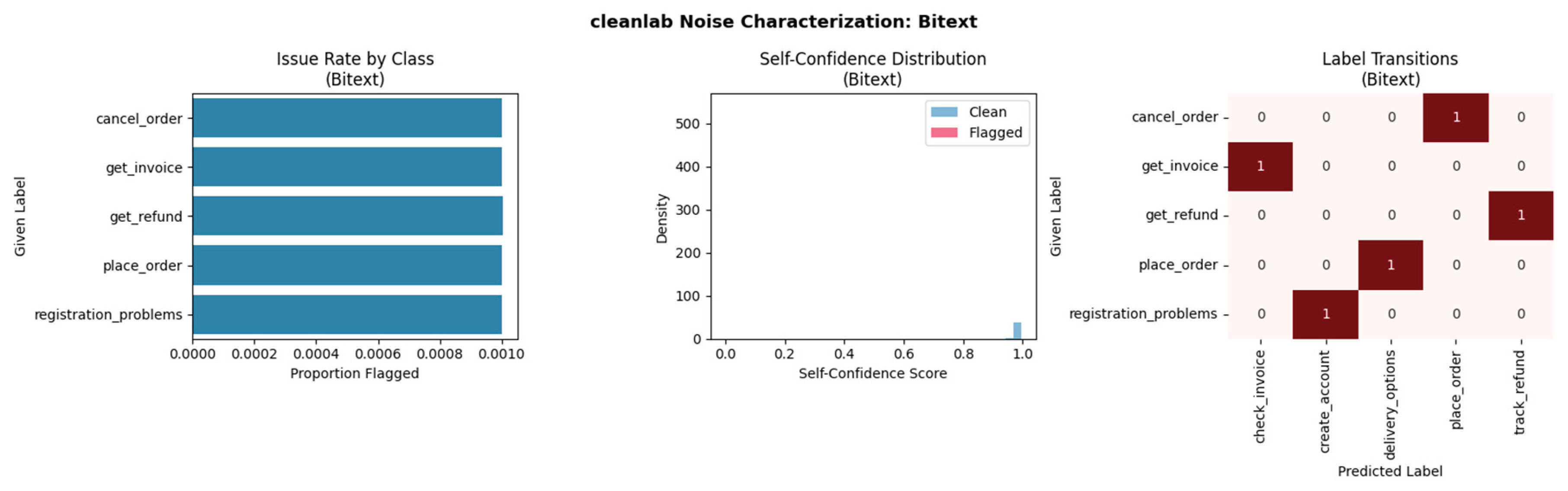
Figure A2.
CLINC150 noise characterization. Note. There were 837 flagged instances identified and the rate of problem instances differed across the 150 problem categories as demonstrated in the ‘Issue Rate by Class’ chart, with some categories flagged at rates above 20% and others below 5%. On an overall basis, the flagged instances exhibited a bimodal distribution pattern and were concentrated in the low self-confidence region.
Figure A2.
CLINC150 noise characterization. Note. There were 837 flagged instances identified and the rate of problem instances differed across the 150 problem categories as demonstrated in the ‘Issue Rate by Class’ chart, with some categories flagged at rates above 20% and others below 5%. On an overall basis, the flagged instances exhibited a bimodal distribution pattern and were concentrated in the low self-confidence region.
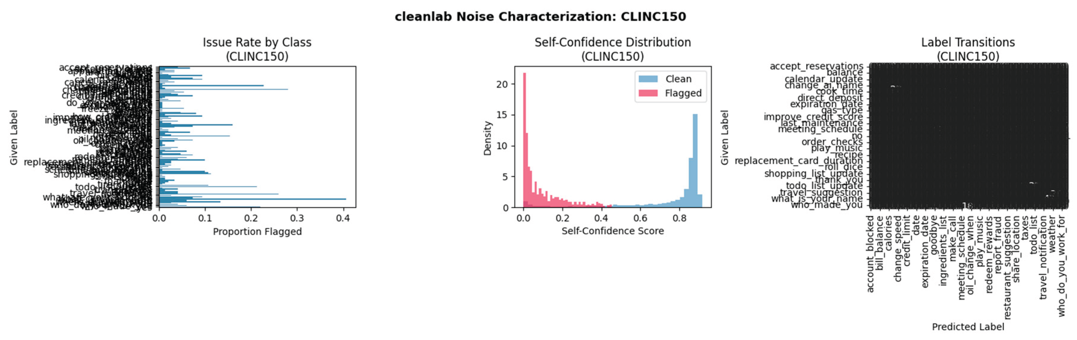
Figure A3.
Kaggle noise characterization. Note. Out of 8469 total entries, there were 4634 flagged as containing an error (54.7%). All five classes had almost equal incidence rates. The distribution of self-confidence appears to have one shape that is broad and unimodal and a central location near the median rather than two distinct shapes that represent a bimodal distribution, which would indicate a cleaner set of data, supporting the conclusion of non-recoverable label noise.
Figure A3.
Kaggle noise characterization. Note. Out of 8469 total entries, there were 4634 flagged as containing an error (54.7%). All five classes had almost equal incidence rates. The distribution of self-confidence appears to have one shape that is broad and unimodal and a central location near the median rather than two distinct shapes that represent a bimodal distribution, which would indicate a cleaner set of data, supporting the conclusion of non-recoverable label noise.
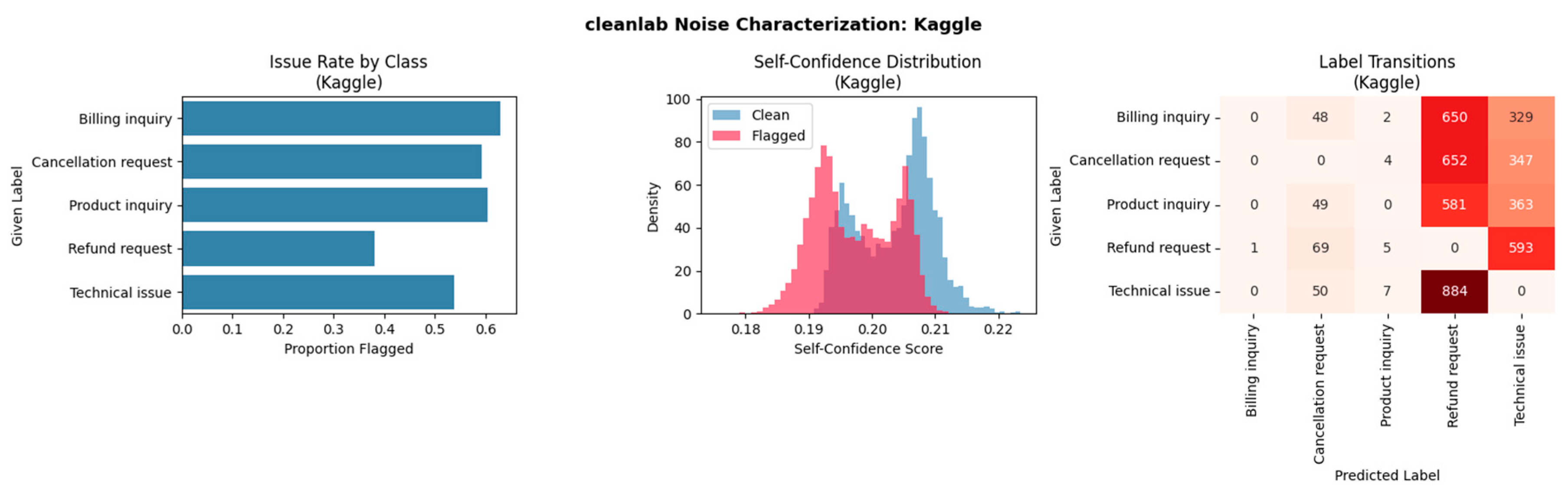
Figure A4.
Yelp noise characterization. Note. A total of 16,941 of the 50,000 reviews (33.9% of the entire corpus) were flagged as having issues. The highest flagging rates are found among 2-star and 4-star rated reviews, indicating the difficulty of differentiating between intermediate levels of sentiment. Adjacent star-ratings show clustering associated with label transitions from one to another.
Figure A4.
Yelp noise characterization. Note. A total of 16,941 of the 50,000 reviews (33.9% of the entire corpus) were flagged as having issues. The highest flagging rates are found among 2-star and 4-star rated reviews, indicating the difficulty of differentiating between intermediate levels of sentiment. Adjacent star-ratings show clustering associated with label transitions from one to another.
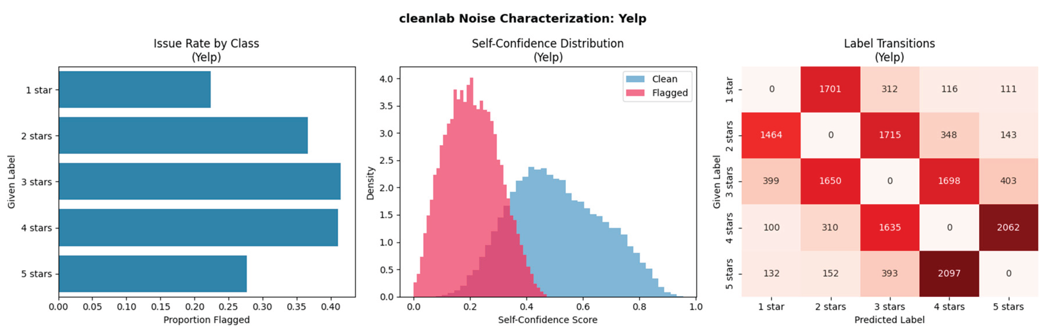
Figure A5.
AG News noise characterization. Note. A total of 699 instances were flagged out of 20,000, which is equal to 3.5% of the total corpus. Each of the 4 categories (World, Sports, Business and Sci/Tech) was flagged at approximately the same rate. The self-confidence distribution is bimodal with a clear division between flagged and unflagged instances.
Figure A5.
AG News noise characterization. Note. A total of 699 instances were flagged out of 20,000, which is equal to 3.5% of the total corpus. Each of the 4 categories (World, Sports, Business and Sci/Tech) was flagged at approximately the same rate. The self-confidence distribution is bimodal with a clear division between flagged and unflagged instances.
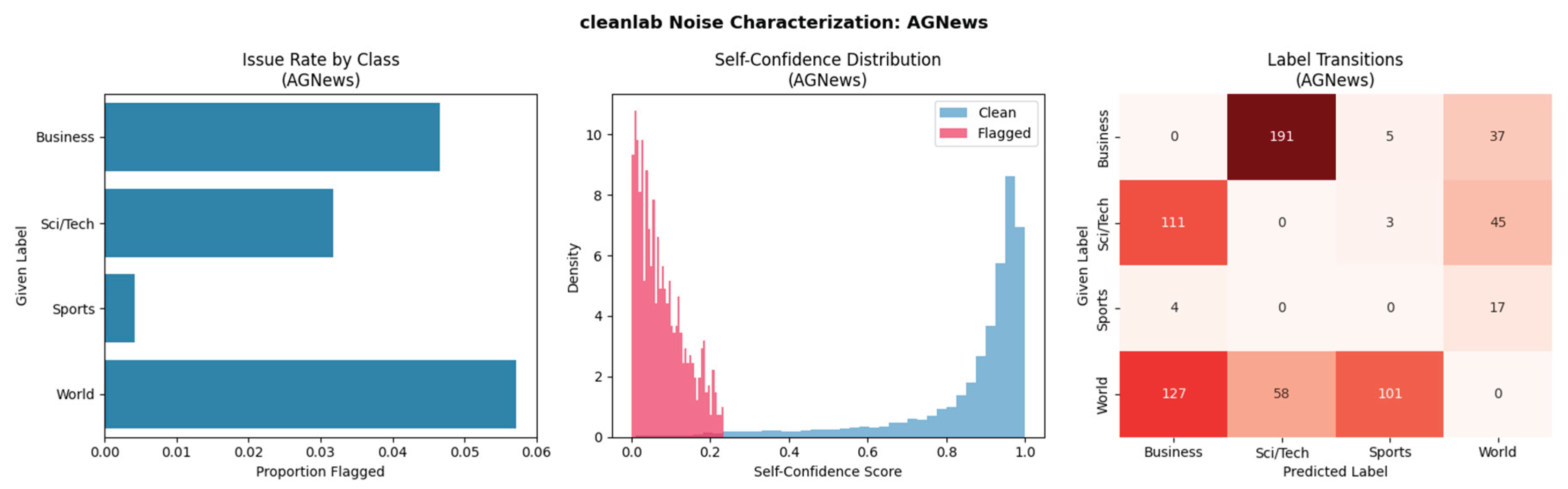
Appendix D. Pilot Study Details
Four models/architectures were evaluated across three different corpora in a pilot study in order to determine whether model capacity governs classification performance. The anomaly that was described in the ‘Origin of the Research Question’ motivated the creation of the controlled experiments reported in the main text. The overall experiment design and the results from each of the corpora are included here for the reader’s information.
In the pilot study conducted by Senne (2026), four different architecture approaches to implementing an intent classification model were used. The different architectures ranged from logistic regression to DistilBERT with pre-trained GloVe embeddings (Pennington, Socher, and Manning 2014). The total number of parameters for the models used in this study ranged over four orders of magnitude. The different architectures were assessed using a stratified training/validation/test split of 70/15/15 for the respective splits of the training/validation/test data, and the metrics used to evaluate the model’s performance were macro F1 score and McNemar’s test (Dietterich 1998) to measure significant differences between the best models. The results produced from the two corpora, the customer support corpus of Bitext (Bitext Innovations 2023) and the CLINC150 intent classification corpus (Larson et al. 2019), supported the relationship between the capacity of the model and its performance, however, the macro F1 score of 0.997 produced by DistilBERT on the Bitext corpus suggests a statistically significant advantage over the BiLSTM model (Hochreiter and Schmidhuber 1997) (chi-squared = 22.13, p < 0.001). Previous research has indicated that descriptive and contextual learning models using embeddings produce superior performance for fine-grained intent classification (Zangari et al. 2023).
A synthetic customer support dataset sourced from Kaggle (Suraj 2023) was used as a third corpus. It was determined that all four architectures failed to achieve any greater than random chance levels of performance in predicting customer satisfaction as none achieved a macro F1-score greater than 0.211. The macro F1-score achieved by each model was between 0.140 and 0.211 and there was no statistically significant difference between the highest scoring models (chi-squared = 0.003, p = 0.954). The findings contradict the hypothesis that transformer architectures could extract meaningful signals from any corpus in which the linguistic structures can be recovered (Devlin et al. 2019; Rogers, Kovaleva, and Rumshisky 2020). The latent Dirichlet allocation analysis revealed six coherent topics when K = 6, C_v = 0.566 (Blei, Ng, and Jordan 2003; Röder, Both, and Hinneburg 2015). Although the coherence score is not strong enough to determine clear class boundaries, it indicates that the structure of inputs is coherent enough to allow parts of the input to be useful to a well-performing classifier. Therefore, since none of the four architectures outperformed random chance for predicting customer satisfaction, one can assume that the issue lies with the classification of the data and not the data itself, indicating that there exists high levels of independence between the supervised labels assigned and the text.
References
- Aguda, T.D.; Siddagangappa, S.; Kochkina, E.; Kaur, S.; Wang, D.; Smiley, C. Large language models as financial data annotators: A study on effectiveness and efficiency. In Proceedings of the 2024 Joint International Conference on Computational Linguistics, Language Resources and Evaluation (LREC-COLING 2024), Turin, Italy, 20–25 May 2024; ELRA and ICCL: Paris, France, 2024; pp. 10124–10145. Available online: https://aclanthology.org/2024.lrec-main.885/.
- Aroyo, L.; Welty, C. Truth is a lie: Crowd truth and the seven myths of human annotation. AI Mag. 2015, 36, 15–24. [Google Scholar] [CrossRef]
- Bitext Innovations. Bitext Customer Support LLM Chatbot Training Dataset. Hugging Face. Accessed June 2026. 2023. Available online: https://huggingface.co/datasets/bitext/Bitext-customer-support-llm-chatbot-training-dataset.
- Blei, D.M.; Ng, A.Y.; Jordan, M.I. Latent Dirichlet allocation. J. Mach. Learn. Res. 2003, 3, 993–1022. [Google Scholar]
- Carlson, N.A.; Burbano, V.C. The use of LLMs to annotate data in management research: Foundational guidelines and warnings. Strateg. Manag. J. 2026, 47, 699–725. [Google Scholar] [CrossRef]
- Chalkidis, I.; Pasini, T.; Zhang, S.; Tomada, L.; Schwemer, S.; Søgaard, A. FairLex: A multilingual benchmark for evaluating fairness in legal text processing. In Proceedings of the 60th Annual Meeting of the Association for Computational Linguistics (Volume 1: Long Papers); Association for Computational Linguistics: Stroudsburg, PA, USA, 2022; pp. 4389–4406. [Google Scholar] [CrossRef]
- DataX Power. Data Annotation Pricing in 2026: Cost per Hour, per Task and per Project. DataX Power Blog. Accessed July 2026. 2026. Available online: https://www.dataxpower.com/blog/data-annotation-pricing-2026.
- Devlin, J.; Chang, M.-W.; Lee, K.; Toutanova, K. BERT: Pre-training of deep bidirectional transformers for language understanding. In Proceedings of the 2019 Conference of the North American Chapter of the Association for Computational Linguistics; Association for Computational Linguistics: Stroudsburg, PA, USA, 2019; pp. 4171–4186. [Google Scholar] [CrossRef]
- Dietterich, T.G. Approximate statistical tests for comparing supervised classification learning algorithms. Neural Comput. 1998, 10, 1895–1923. [Google Scholar] [CrossRef]
- Donhauser, N.; Fehle, J.; Hellwig, N.C.; Weinberger, M.; Kruschwitz, U.; Wolff, C. Annotation quality in aspect-based sentiment analysis: A case study comparing experts, students, crowdworkers, and large language model. arXiv 2026, arXiv:2605.03624. [Google Scholar] [CrossRef]
- Frénay, B.; Verleysen, M. Classification in the presence of label noise: A survey. IEEE Trans. Neural Netw. Learn. Syst. 2014, 25, 845–869. [Google Scholar] [CrossRef]
- Geman, S.; Bienenstock, E.; Doursat, R. Neural networks and the bias/variance dilemma. Neural Comput. 1992, 4, 1–58. [Google Scholar] [CrossRef]
- Gilardi, F.; Alizadeh, M.; Kubli, M. ChatGPT outperforms crowd workers for text-annotation tasks. Proc. Natl. Acad. Sci. USA 2023, 120, e2305016120. [Google Scholar] [CrossRef] [PubMed]
- Google Cloud. Accelerator-Optimized VM Pricing. Google Cloud Documentation. Accessed July 2026. 2026. Available online: https://cloud.google.com/products/compute/pricing/accelerator-optimized.
- Hastie, T.; Tibshirani, R.; Friedman, J. The Elements of Statistical Learning: Data Mining, Inference, and Prediction, 2nd ed.; Springer: New York, NY, USA, 2009. [Google Scholar]
- He, X.; Zhao, K.; Chu, X. AutoML: A survey of the state-of-the-art. Knowl.-Based Syst. 2021, 212, 106622. [Google Scholar] [CrossRef]
- Hochreiter, S.; Schmidhuber, J. Long short-term memory. Neural Comput. 1997, 9, 1735–1780. [Google Scholar] [CrossRef] [PubMed]
- Jain, A.; Patel, H.; Nagle, L.; Gupta, N.; Mehta, S.; Guttula, S.; Mujumdar, S.; Afzal, S.; Mittal, R.S.; Munigala, V. Overview and importance of data quality for machine learning tasks. In Proceedings of the 26th ACM SIGKDD International Conference on Knowledge Discovery and Data Mining; Association for Computing Machinery: New York, NY, USA, 2020; pp. 3561–3562. [Google Scholar] [CrossRef]
- Kang, J.; Xu, W.; Ritter, A. Distill or annotate? Cost-efficient fine-tuning of compact models. In Proceedings of the 61st Annual Meeting of the Association for Computational Linguistics (Volume 1: Long Papers); Association for Computational Linguistics: Toronto, Canada, 2023; pp. 11100–11119. [Google Scholar] [CrossRef]
- Klie, J.-C.; de Castilho, R.E.; Gurevych, I. Analyzing dataset annotation quality management in the wild. Comput. Linguist. 2024, 50, 817–866. [Google Scholar] [CrossRef]
- Larson, S.; Mahendran, A.; Peper, J.J.; Clarke, C.; Lee, A.; Hill, P.; Kummerfeld, J.K.; Leach, K.; Laurenzano, M.A.; Tang, L.; et al. An evaluation dataset for intent classification and out-of-scope prediction. In Proceedings of the 2019 Conference on Empirical Methods in Natural Language Processing and the 9th International Joint Conference on Natural Language Processing; Association for Computational Linguistics: Stroudsburg, PA, USA, 2019; pp. 1311–1316. [Google Scholar] [CrossRef]
- Liu, Y.; Ott, M.; Goyal, N.; Du, J.; Joshi, M.; Chen, D.; Levy, O.; Lewis, M.; Zettlemoyer, L.; Stoyanov, V. RoBERTa: A robustly optimized BERT pretraining approach. arXiv 2019, arXiv:1907.11692. [Google Scholar] [CrossRef]
- Ng, A. A Chat with Andrew on MLOps: From Model-Centric to Data-Centric AI. DeepLearning.AI, March 24, 2021. YouTube Video, 1:13:48. 2021. Available online: https://www.youtube.com/watch?v=06-AZXmwHjo.
- Northcutt, C.G.; Jiang, L.; Chuang, I.L. Confident learning: Estimating uncertainty in dataset labels. J. Artif. Intell. Res. 2021, 70, 1373–1411. [Google Scholar] [CrossRef]
- Pennington, J.; Socher, R.; Manning, C.D. GloVe: Global vectors for word representation. In Proceedings of the 2014 Conference on Empirical Methods in Natural Language Processing; Association for Computational Linguistics: Stroudsburg, PA, USA, 2014; pp. 1532–1543. [Google Scholar] [CrossRef]
- Ratul, M.T.R.; Chen, Z.; Fu, K.; Ji, T.; Zhang, L. MasterSet: A large-scale benchmark for must-cite citation recommendation in the AI/ML literature. arXiv 2026, arXiv:2604.17680. [Google Scholar] [CrossRef]
- Renggli, C.; Rimanic, L.; Gürel, N.M.; Karlaš, B.; Wu, W.; Zhang, C. A data quality-driven view of MLOps. IEEE Data Eng. Bull. 2021, 44, 11–23. Available online: http://sites.computer.org/debull/A21mar/p11.pdf.
- Röder, M.; Both, A.; Hinneburg, A. Exploring the space of topic coherence measures. In Proceedings of the Eighth ACM International Conference on Web Search and Data Mining; Association for Computing Machinery: New York, NY, USA, 2015; pp. 399–408. [Google Scholar] [CrossRef]
- Rogers, A.; Kovaleva, O.; Rumshisky, A. A primer in BERTology: What we know about how BERT works. Trans. Assoc. Comput. Linguist. 2020, 8, 842–866. [Google Scholar] [CrossRef]
- Sambasivan, N.; Kapania, S.; Highfill, H.; Akrong, D.; Paritosh, P.; Aroyo, L.M. Everyone wants to do the model work, not the data work: Data cascades in high-stakes AI. In Proceedings of the 2021 CHI Conference on Human Factors in Computing Systems; Association for Computing Machinery: New York, NY, USA, 2021; pp. 1–15. [Google Scholar] [CrossRef]
- Sanh, V.; Debut, L.; Chaumond, J.; Wolf, T. DistilBERT, a distilled version of BERT: Smaller, faster, cheaper and lighter. arXiv 2019, arXiv:1910.01108. [Google Scholar] [CrossRef]
- Schwartz, R.; Dodge, J.; Smith, N.A.; Etzioni, O. Green AI. Commun. ACM 2020, 63, 5–63. [Google Scholar] [CrossRef]
- Senne, J. Comparative Study of ML and Transformer Models for Customer Support Intent Classification. Unpublished Manuscript, Northwestern University. Northwestern University, 2026.
- Snow, R.; O’Connor, B.; Jurafsky, D.; Ng, A.Y. Cheap and fast, but is it good? Evaluating non-expert annotations for natural language tasks. In Proceedings of the 2008 Conference on Empirical Methods in Natural Language Processing; Association for Computational Linguistics: Stroudsburg, PA, USA, 2008; pp. 254–263. Available online: https://aclanthology.org/D08-1027/.
- Song, H.; Kim, M.; Park, D.; Shin, Y.; Lee, J.-G. Learning from noisy labels with deep neural networks: A survey. IEEE Trans. Neural Netw. Learn. Syst. 2022, 34, 8135–8153. [Google Scholar] [CrossRef]
- Suraj. Customer Support Ticket Dataset. Kaggle. 2023. Available online: https://www.kaggle.com/datasets/suraj520/customer-support-ticket-dataset.
- Vaswani, A.; Shazeer, N.; Parmar, N.; Uszkoreit, J.; Jones, L.; Gomez, A.N.; Kaiser, Ł.; Polosukhin, I. Attention is all you need. In Advances in Neural Information Processing Systems; The MIT Press: Cambridge, MA, USA, 2017; Volume 30, pp. 5998–6008. Available online: https://papers.nips.cc/paper/2017/hash/3f5ee243547dee91fbd053c1c4a845aa-Abstract.html.
- Wei, J.; Zhu, Z.; Cheng, H.; Liu, T.; Niu, G.; Liu, Y. Learning with noisy labels revisited: A study using real-world human annotations. In Proceedings of the International Conference on Learning Representations, Virtual, 25–29 April 2022; Available online: https://openreview.net/forum?id=TBWA6PLJZQm.
- Whang, S.E.; Roh, Y.; Song, H.; Lee, J.-G. Data collection and quality challenges in deep learning: A data-centric AI perspective. VLDB J. 2023, 32, 791–813. [Google Scholar] [CrossRef]
- Xie, Q.; Luong, M.-T.; Hovy, E.; Le, Q.V. Self-training with noisy student improves ImageNet classification. In Proceedings of the IEEE/CVF Conference on Computer Vision and Pattern Recognition, Seattle, WA, USA, 13–19 June 2020; pp. 10687–10698. [Google Scholar] [CrossRef]
- Zangari, A.; Marcuzzo, M.; Schiavinato, M.; Gasparetto, A.; Albarelli, A. Ticket automation: An insight into current research with applications to multi-level classification scenarios. Expert Syst. Appl. 2023, 225, 119984. [Google Scholar] [CrossRef]
- Zha, D.; Bhat, Z.P.; Lai, K.-H.; Yang, F.; Jiang, Z.; Zhong, S.; Hu, X. Data-centric artificial intelligence: A survey. arXiv 2023, arXiv:2303.10158. [Google Scholar] [CrossRef]
- Zhang, C.; Bengio, S.; Hardt, M.; Recht, B.; Vinyals, O. Understanding deep learning requires rethinking generalization. Proceedings of the International Conference on Learning Representations, Toulon, France, 24–26 April 2017; Available online: https://openreview.net/forum?id=Sy8gdB9xx.
- Zhang, X.; Zhao, J.; LeCun, Y. Character-level convolutional networks for text classification. Adv. Neural Inf. Process. Syst. 28 2015, 649–657. Available online: https://papers.nips.cc/paper/2015/hash/250cf8b51c773f3f8dc8b4be867a9a02-Abstract.html.
- Zhu, Y.; Xie, Y.; Zhou, X.; Liu, Y.; Sun, X. Bringing order to chaos: Preventing label noise learning from non-convergence. In Proceedings of the 60th Annual Meeting of the Association for Computational Linguistics (Volume 1: Long Papers); Association for Computational Linguistics: Dublin, Ireland, 2022; pp. 4234–4245. [Google Scholar] [CrossRef]
Figure 8.
Confident learning detection performance on CIFAR-N validation set. Note. Detection performance was measured under 12 different conditions, which are made up of 2 different noise types at 6 different injection rates. CIFAR-10 was used as the base corpus and noise was injected against known ground truth labels provided by Wei et al. (2022). The estimator used was the calibrated LinearSVC, which is a support vector classifier, and used TF-IDF features (maximum of 20,000 features) in addition to bigram n-grams. The out-of-sample predicted probabilities were generated through use of five-fold cross-validation. As per the baseline defined by Northcutt, Jiang, and Chuang (2021), detection reliability degrades below the 25% noise ceiling.
Figure 8.
Confident learning detection performance on CIFAR-N validation set. Note. Detection performance was measured under 12 different conditions, which are made up of 2 different noise types at 6 different injection rates. CIFAR-10 was used as the base corpus and noise was injected against known ground truth labels provided by Wei et al. (2022). The estimator used was the calibrated LinearSVC, which is a support vector classifier, and used TF-IDF features (maximum of 20,000 features) in addition to bigram n-grams. The out-of-sample predicted probabilities were generated through use of five-fold cross-validation. As per the baseline defined by Northcutt, Jiang, and Chuang (2021), detection reliability degrades below the 25% noise ceiling.
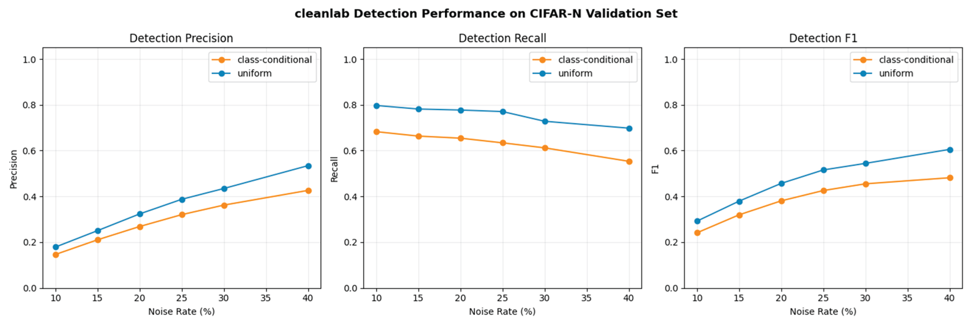
Figure 9.
Performance-quality curves by corpus and remediation strategy. Note. Macro F1 (y-axis) for the three architectures is plotted against remediation threshold (x-axis). The shaded areas indicate the variability of the results across five stratified cross-validation folds (i.e., ±1 standard deviation). The rows of the panels are arranged in order of increasing detected noise rate. Removal strategy for the left column, relabeling strategy for the right column. None of the architectures in Kaggle have achieved above 0.28 for macro F1 at any threshold regardless of strategy; this is barely above random chance for a five-class problem.
Figure 9.
Performance-quality curves by corpus and remediation strategy. Note. Macro F1 (y-axis) for the three architectures is plotted against remediation threshold (x-axis). The shaded areas indicate the variability of the results across five stratified cross-validation folds (i.e., ±1 standard deviation). The rows of the panels are arranged in order of increasing detected noise rate. Removal strategy for the left column, relabeling strategy for the right column. None of the architectures in Kaggle have achieved above 0.28 for macro F1 at any threshold regardless of strategy; this is barely above random chance for a five-class problem.
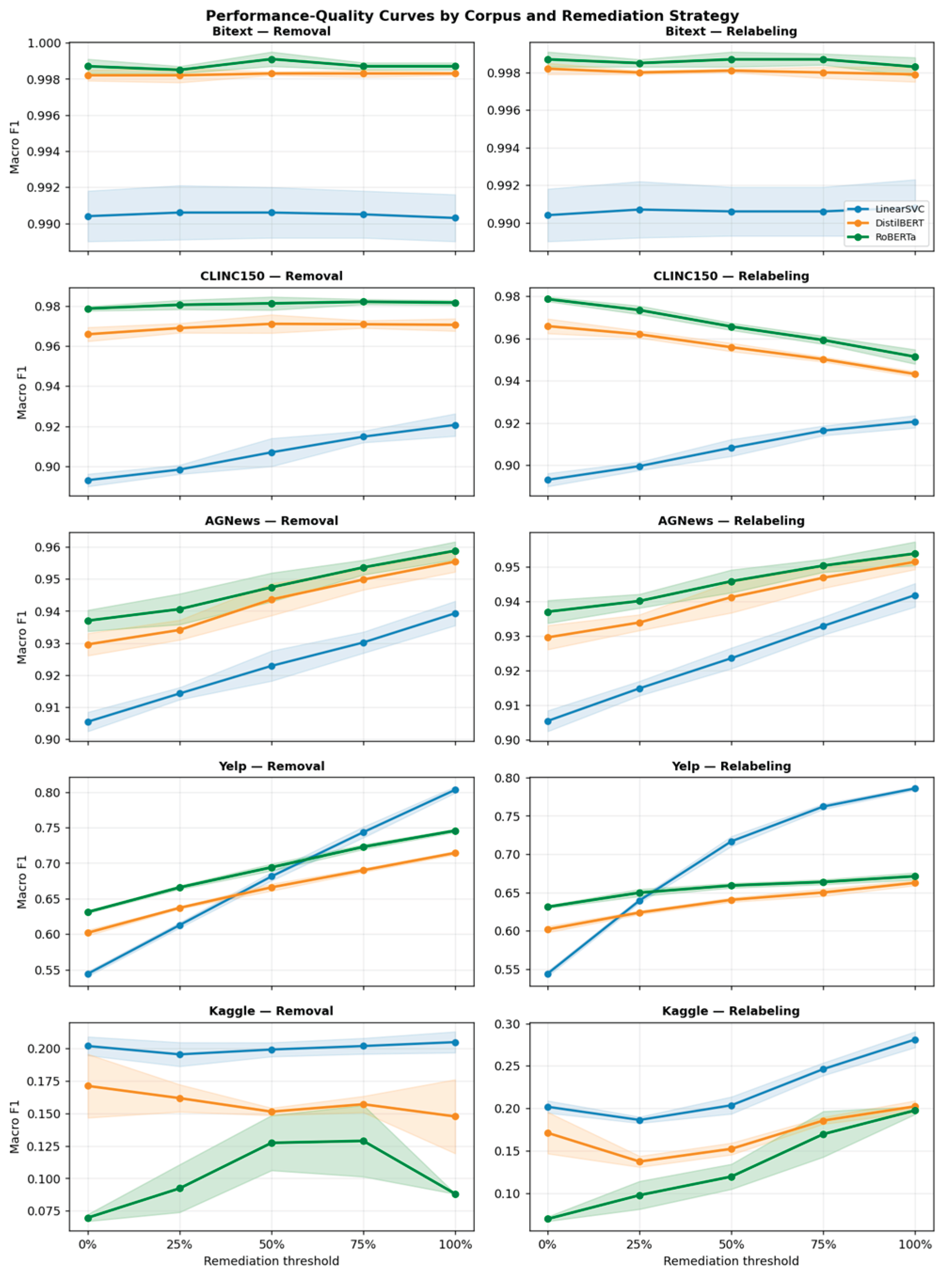
Figure 10.
Architecture divergence by corpus: fraction of Bonferroni-significant pairwise comparisons. Note. Each cell provides the proportion of significant differences from Bonferroni Adjusted alpha (0.000333) across 150 pairwise comparison tests conducted under five different thresholds using two separate remediation strategies. Higher proportions indicate that the architecture performs significantly different than each other using the data set in question. All LinearSVC associations on the CLINC150 data set are significantly different than either transformer, while in contrast, there is very little statistical support that DistilBERT and RoBERTa are significantly different than one another (only 20%). On the Kaggle data set, DistilBERT and RoBERTa have no significant differences across the data set, reflecting their shared failure mode.
Figure 10.
Architecture divergence by corpus: fraction of Bonferroni-significant pairwise comparisons. Note. Each cell provides the proportion of significant differences from Bonferroni Adjusted alpha (0.000333) across 150 pairwise comparison tests conducted under five different thresholds using two separate remediation strategies. Higher proportions indicate that the architecture performs significantly different than each other using the data set in question. All LinearSVC associations on the CLINC150 data set are significantly different than either transformer, while in contrast, there is very little statistical support that DistilBERT and RoBERTa are significantly different than one another (only 20%). On the Kaggle data set, DistilBERT and RoBERTa have no significant differences across the data set, reflecting their shared failure mode.
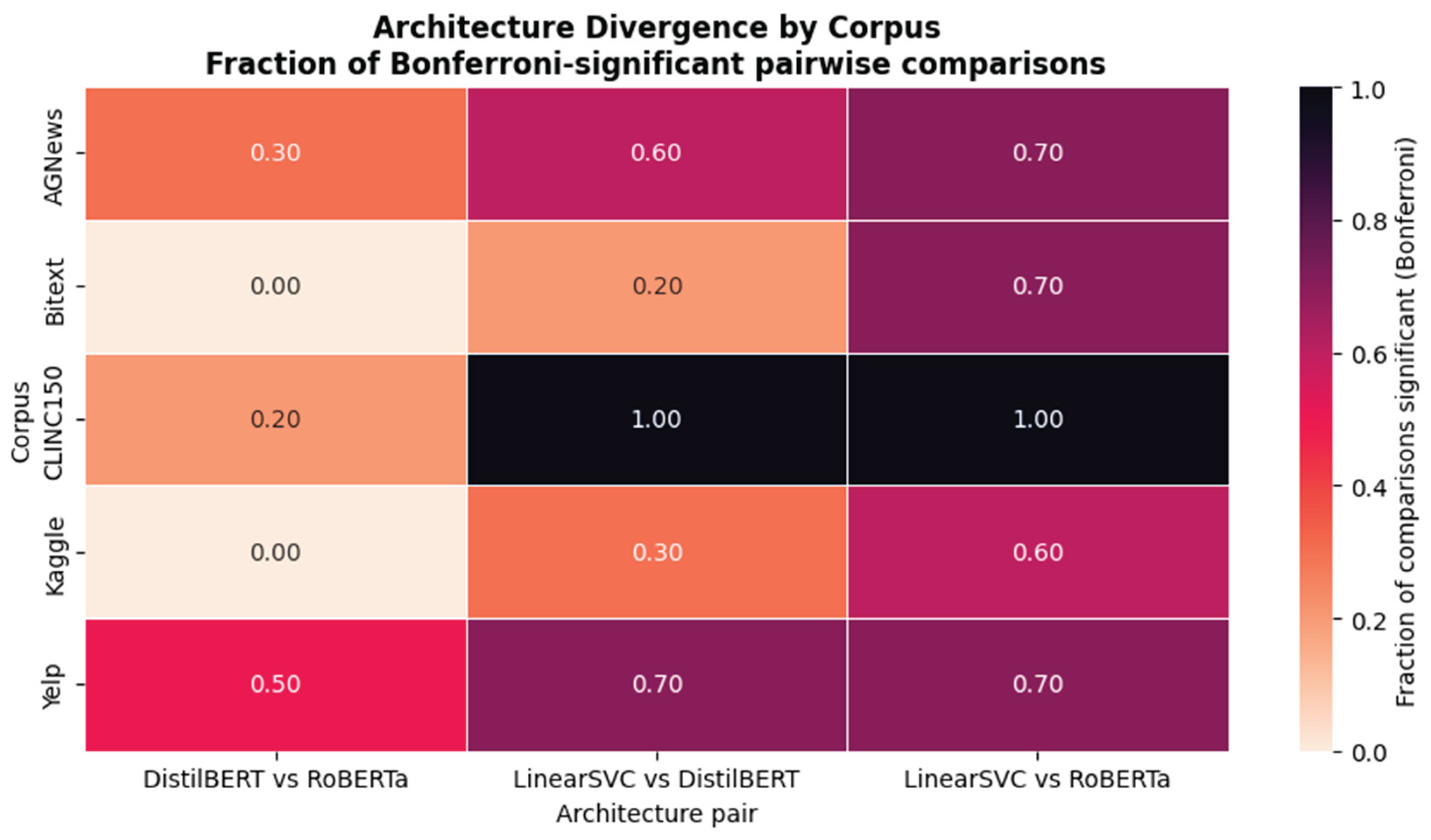
Figure 11.
Divergence rate by remediation threshold. Note. The panels show the ratio of Bonferroni significant comparisons for all pairwise architecture comparisons at each remediation level for both strategies. The y-axis represents the ratio of the three pairwise architecture comparisons that were determined to be Bonferroni significant at each of these remediation levels. The 0% relabeling condition is omitted because it is definitionally identical to the 0% removal condition. For Yelp, both strategies produce high architecture divergence at the 0% threshold and again at 75% and 100%. This indicates that, at the mid-point of remediation, the architecture crossover happens.
Figure 11.
Divergence rate by remediation threshold. Note. The panels show the ratio of Bonferroni significant comparisons for all pairwise architecture comparisons at each remediation level for both strategies. The y-axis represents the ratio of the three pairwise architecture comparisons that were determined to be Bonferroni significant at each of these remediation levels. The 0% relabeling condition is omitted because it is definitionally identical to the 0% removal condition. For Yelp, both strategies produce high architecture divergence at the 0% threshold and again at 75% and 100%. This indicates that, at the mid-point of remediation, the architecture crossover happens.
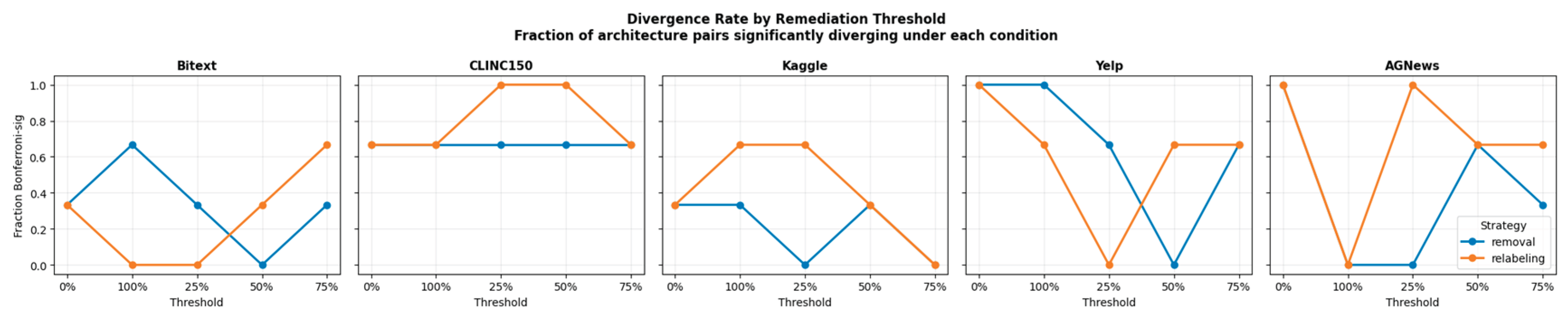
Figure 12.
Per-corpus Pareto frontiers at $0.40 per instance annotation rate. Note. Marker shapes illustrate remediation strategies; circles indicate removal; while triangles indicate relabeling. Additionally, marker colors illustrate types of architectures; with steelblue indicating LinearSVC, orange indicating DistilBERT, and green indicating RoBERTa. The x-axis uses a logarithmic scale and represents the combined USD total cost of compute (i.e., Google Cloud A100 at $3.67 per hour) and annotation (relabeling only $0.40 per remediated instance). The dashed crimson line connects the non-dominated conditions that form the Pareto frontier for each corpus. For all removal conditions, the annotation/labeling cost is $0 (regardless of threshold). For the Yelp and Kaggle frontiers they are dominated by the LinearSVC conditions; whereas for the Bitext, CLINC150, and AG News, all three architectures are represented in the Pareto frontier.
Figure 12.
Per-corpus Pareto frontiers at $0.40 per instance annotation rate. Note. Marker shapes illustrate remediation strategies; circles indicate removal; while triangles indicate relabeling. Additionally, marker colors illustrate types of architectures; with steelblue indicating LinearSVC, orange indicating DistilBERT, and green indicating RoBERTa. The x-axis uses a logarithmic scale and represents the combined USD total cost of compute (i.e., Google Cloud A100 at $3.67 per hour) and annotation (relabeling only $0.40 per remediated instance). The dashed crimson line connects the non-dominated conditions that form the Pareto frontier for each corpus. For all removal conditions, the annotation/labeling cost is $0 (regardless of threshold). For the Yelp and Kaggle frontiers they are dominated by the LinearSVC conditions; whereas for the Bitext, CLINC150, and AG News, all three architectures are represented in the Pareto frontier.
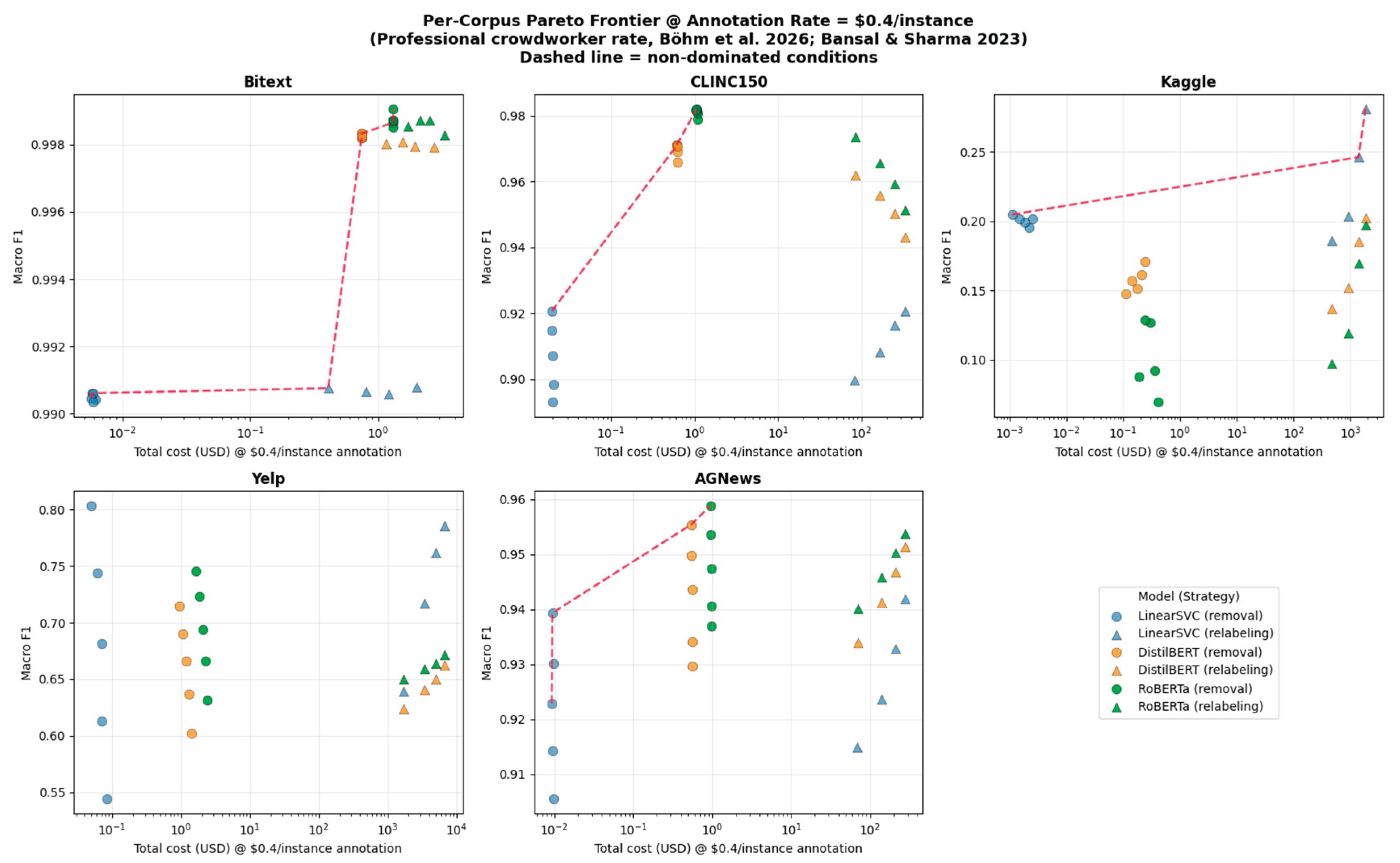
Figure 13.
Pareto frontier sensitivity across the 2025 to 2026 annotation rate landscape. Note. It includes the LLM economical tier ($0.0003/instance) on top and the LLM frontier (or crowd floor) tier ($0.10/instance) just below it, with the professional crowdworker rate ($0.40/instance) below that and the expert human rate ($2.00/instance) on the bottom. Each annotation tier is compared using the same 27 conditions for each corpus as in Figure 9. The only difference is that the cost of annotating each set of conditions varies by the annotation tier. The dashed crimson line connects the non-dominated conditions for a given tier/corpus combination. As the annotation rate rises, the frontier shifts toward removal-dominated conditions.
Figure 13.
Pareto frontier sensitivity across the 2025 to 2026 annotation rate landscape. Note. It includes the LLM economical tier ($0.0003/instance) on top and the LLM frontier (or crowd floor) tier ($0.10/instance) just below it, with the professional crowdworker rate ($0.40/instance) below that and the expert human rate ($2.00/instance) on the bottom. Each annotation tier is compared using the same 27 conditions for each corpus as in Figure 9. The only difference is that the cost of annotating each set of conditions varies by the annotation tier. The dashed crimson line connects the non-dominated conditions for a given tier/corpus combination. As the annotation rate rises, the frontier shifts toward removal-dominated conditions.
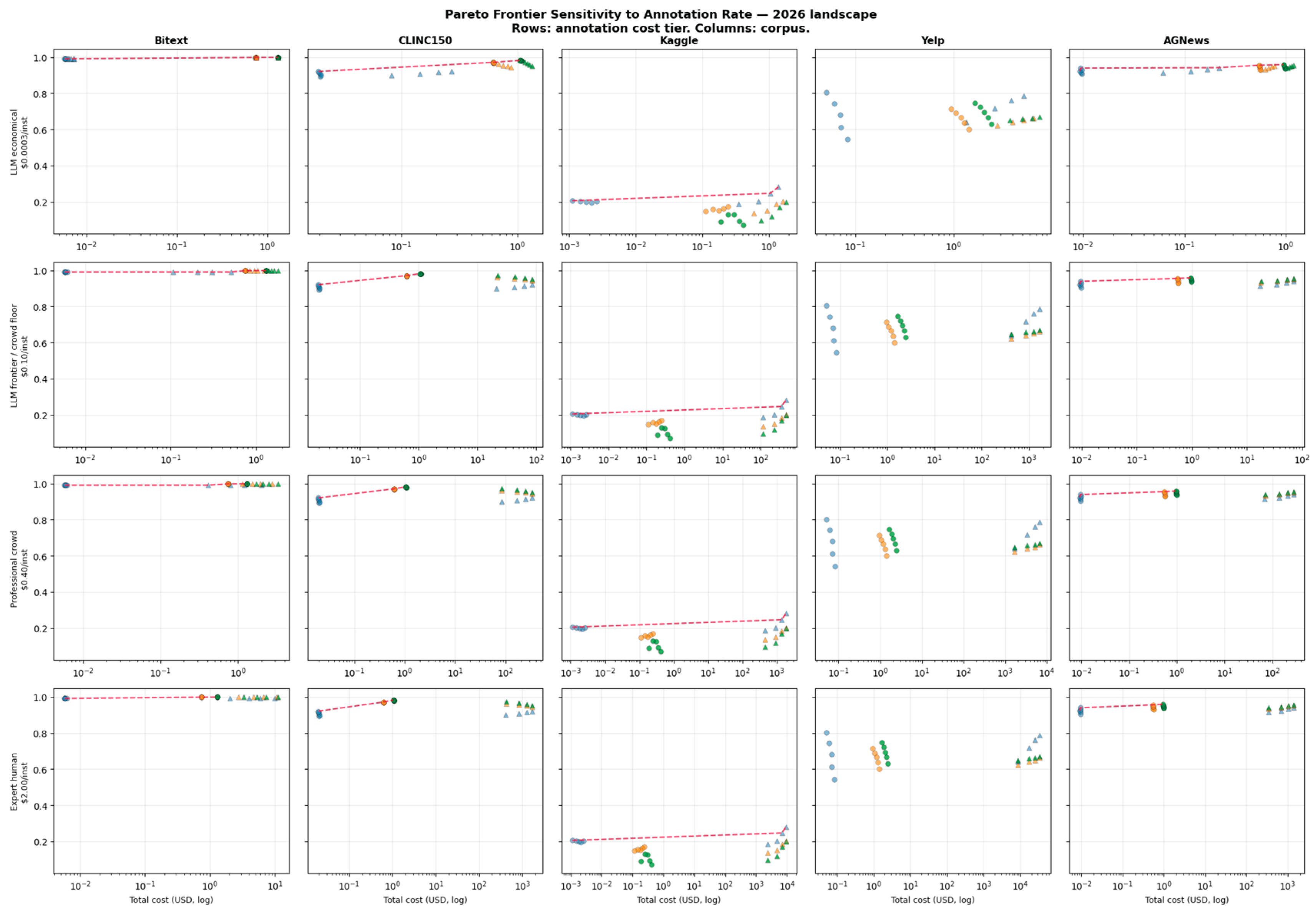
Figure 14.
Practitioner decision framework for architecture and remediation strategy selection. Note. The framework is relevant only to text classification tasks where confident learning detection can be run as a diagnostic step. The noise rates that have been detected need to be assessed according to the CIFAR-N reliability floor shown in Figure 8. If the diagnostic reveals catastrophic noise and a uniformly architecturally failed model, this indicates the need for an examination of the labeling procedure and not an analysis of architectural or remediation solutions.
Figure 14.
Practitioner decision framework for architecture and remediation strategy selection. Note. The framework is relevant only to text classification tasks where confident learning detection can be run as a diagnostic step. The noise rates that have been detected need to be assessed according to the CIFAR-N reliability floor shown in Figure 8. If the diagnostic reveals catastrophic noise and a uniformly architecturally failed model, this indicates the need for an examination of the labeling procedure and not an analysis of architectural or remediation solutions.
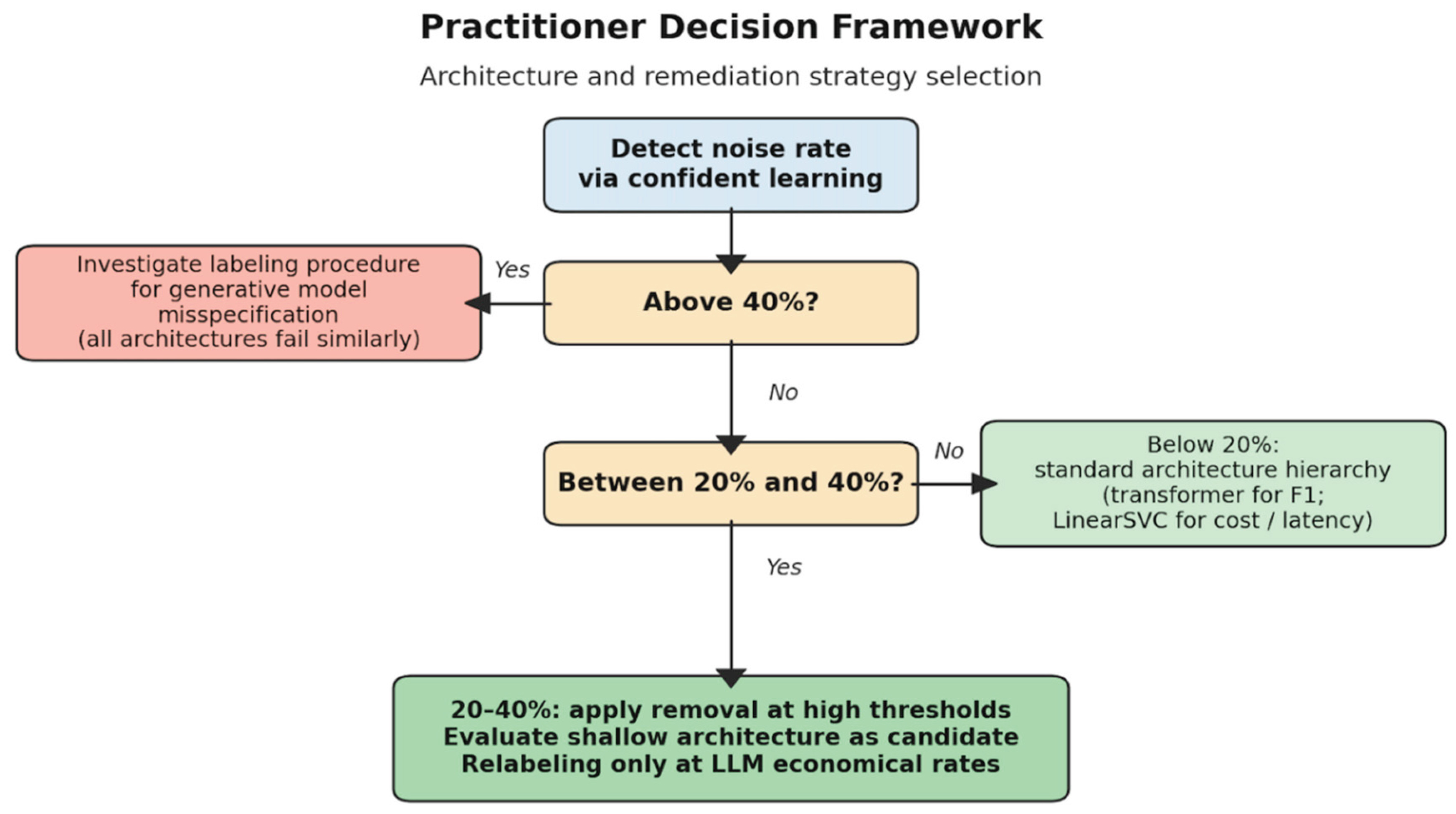
Table 2.
Corpus characteristics and detected label noise rates.
| Corpus | Instances | Classes | Detected Noise Rate | Regime |
|---|---|---|---|---|
| Bitext | 26,872 | 27 | 0.0% | Clean baseline |
| AG News | 20,000 | 4 | 3.5% | Low, professional text |
| CLINC150 | 22,500 | 150 | 3.7% | Low, fine-grained intent |
| Yelp Review Full | 50,000 | 5 | 33.9% | Moderate, natural noise |
| Kaggle Customer Support | 8469 | 5 | 54.7% | Catastrophic, synthetic |
Note. Sources: Bitext Innovations (2023); AG News and Yelp Review Full are from Zhang, Zhao, and LeCun (2015); The CLINC150 data used is from Larson et al. (2019) and the Kaggle data used is from Suraj (2023). The noise detection percentage is the percentage of instances flagged by the cleanlab version 2.0 tool as possibly mislabeled, computed based on the joint distribution estimation outlined in Northcutt, Jiang, and Chuang (2021). The AG News and Yelp Review datasets were downsampled to 20,000 and 50,000 instances respectively to limit compute expenses while maintaining the overall number of samples per class (i.e., stratified sampling).
Table 6.
Confident learning noise detection outcomes across the five corpora.
| Corpus | Instances | Issues Detected | Detected Noise Rate |
|---|---|---|---|
| Bitext | 26,872 | 5 | 0.0% |
| AG News | 20,000 | 699 | 3.5% |
| CLINC150 | 22,500 | 837 | 3.7% |
| Yelp Review Full | 50,000 | 16,941 | 33.9% |
| Kaggle Customer Support | 8469 | 4634 | 54.7% |
Note. Cleanlab library (version 2.0) was used for the noise detection process with a calibrated LinearSVC using TF-IDF features (20,000 max features, bigram n-grams, minimum document frequency of 2) as the base estimator; out-of-sample predicted probabilities were produced using five-fold stratified cross-validation; Kaggle’s detection rate is above the validated region for CIFAR-N and should be interpreted using the extrapolation caveat noted in the section ‘CIFAR-N Detection Reliability Validation’.
Disclaimer/Publisher’s Note: The statements, opinions and data contained in all publications are solely those of the individual author(s) and contributor(s) and not of MDPI and/or the editor(s). MDPI and/or the editor(s) disclaim responsibility for any injury to people or property resulting from any ideas, methods, instructions or products referred to in the content. |
© 2026 by the authors. Licensee MDPI, Basel, Switzerland. This article is an open access article distributed under the terms and conditions of the Creative Commons Attribution (CC BY) license (http://creativecommons.org/licenses/by/4.0/).
Copyright: This open access article is published under a Creative Commons CC BY 4.0 license, which permit the free download, distribution, and reuse, provided that the author and preprint are cited in any reuse.