Constraint Qualifications and Optimality Conditions for Nonsmooth Interval-Valued Multiobjective Programming Problems with Vanishing Constraints on Hadamard Manifolds

1. Introduction

In optimization theory, the concept of mathematical programming problems with vanishing constraints (MPVCs) originates from the work of Achtziger and Kanzow [1]. The terminology vanishing constraints describes a structural property whereby, at certain feasible points, some constraints vanish or lose their relevance (see, for instance, [1,2]). One of the main difficulties associated with MPVCs is the non-convex nature of their feasible set, even in the presence of convex constraint functions (see, [3]). Moreover, in general, some of the standard constraint qualifications, namely the Mangasarian-Fromovitz constraint qualification (MFCQ) and linearly independent constraint qualification (LICQ), typically fail to hold at an arbitrary feasible point of MPVCs (see, for instance, [4]). Despite these challenges, MPVCs have several real-life applications in science and engineering, including topology design problems in mechanical structures [1] and robot path-finding problems (see, [5]). Constraint qualifications as well as optimality conditions for smooth multiobjective MPVCs have been established by Mishra et al. [6]. Moreover, Sadeghieh et al. [7] derived necessary and sufficient optimality conditions for nonsmooth multiobjective MPVCs via Clarke subdifferentials. For nonsmooth multiobjective MPVCs, Antczak [8] developed KKT-type necessary optimality conditions by employing a modified Cottle-type constraint qualification in terms of Clarke subdifferentials.

Various optimization problems arising in engineering, economics, and computer science often deal with uncertain data caused by measurement inaccuracies or variations in market behavior (see, for instance, [9,10]). In order to address these uncertainties in optimization problems, several optimization approaches, namely stochastic optimization, fuzzy optimization, and interval-valued optimization have been widely investigated (see, [11,12,13,14]). Due to the difficulties in finding a probability distribution function or a fuzzy membership function in stochastic and fuzzy optimization techniques, respectively, interval-valued optimization has emerged as a significant approach over stochastic and fuzzy optimization (see, for instance, [15,16,17,18,19,20,21]). The KKT-type sufficient optimality conditions for multiobjective interval-valued optimization problems involving differentiable functions have been studied by Wu [13]. Moreover, under the generalized Hukuhara differentiability assumptions, Singh et al. [22] established KKT-type optimality conditions for optimization problems involving multiple interval-valued objective functions. Optimality and duality results for interval-valued multiobjective programming problems involving nondifferentiable convex functions have been derived by Antczak [23].

Over the last few decades, researchers have recognized the vital need for employing non-Euclidean geometry, such as Riemannian geometry, to handle complex data structures (see, for instance, [24,25]). In particular, the application of Euclidean geometry in the analysis of symmetric positive definite (SPD) matrices may lead to misleading results and give rise to the so-called swelling effect (see, [26]). This swelling effect introduces spurious results by inflating the determinants of SPD matrices and can also distort the results of commonly used methods (see, [27]). Computing interpolations and averages of SPD matrices can break physical conservation laws if performed under Euclidean geometry (see, for instance, [28]). Furthermore, it has been recognized that several optimization problems emerging in engineering and science are more suitably modeled in the Riemannian manifold setting, rather than in the Euclidean space framework (see, for instance, [24,29] and the references cited therein). Generalizing various optimization techniques from the Euclidean space setting to Riemannian and Hadamard manifolds provides several key benefits. For instance, optimization problems that are non-convex in the Euclidean space framework can be reformulated as convex problems on Riemannian manifolds by employing an appropriate Riemannian metric (see, [30]). Furthermore, constrained optimization problems in the Euclidean space framework can be reformulated as unconstrained optimization problems in the Riemannian manifold setting, thereby allowing the incorporation of Riemannian geometry and the development of more accurate and efficient algorithms (see, [24,31]). Consequently, optimization on manifolds has emerged as an interesting area of research (see, for instance, [32,33,34]).

In the Hadamard manifold setting, Chen [35] has investigated KKT-type optimality conditions for smooth scalar objective interval-valued optimization problems. Ghosh et al. [36] have investigated constraint qualifications and optimality conditions for differentiable multiobjective optimization problems on Hadamard manifolds. Various constraint qualifications for multiobjective MPVCs involving differentiable functions in the Hadamard manifold setting have been studied by Upadhyay and Ghosh [37]. Moreover, Nguyen et al. [38] have derived necessary optimality conditions for unconstrained interval-valued optimization problems and investigated the existence of efficient points by employing the steepest descent algorithm in the Hadamard manifold framework.

Nonsmooth analysis on manifolds has gained substantial attention over the past few decades (see, for instance, [39,40]). This growing interest is primarily driven by the prevalence of nonsmooth functions on manifolds in many real-world optimization problems, such as control theory [41] and matrix analysis [42]. Hosseini [43] has investigated optimality conditions for nonsmooth constrained optimization problems involving locally Lipschitz continuous functions in the setting of complete Riemannian manifolds via Clarke subdifferentials. Further, Upadhyay et al. [44] have investigated constraint qualifications and optimality conditions for the nonsmooth case of multiobjective optimization problems by utilizing Clarke subdifferentials in the setting of Hadamard manifolds.

Constraint qualifications and necessary optimality conditions for various nonlinear programming problems involving multiple interval-valued objective functions in the Euclidean space setting have been extensively studied in the existing literature (see, for instance, [13,22,23] and the references cited therein). Moreover, significant progress has been made in the investigation of constraint qualifications and optimality criteria for multiobjective as well as interval-valued multiobjective optimization problems in the Hadamard manifold setting (see, for instance, [33,35,37,38,44] and the references cited therein). However, there is no research paper that deals with the constraint qualifications and optimality conditions for nonsmooth interval-valued multiobjective programming problems with vanishing constraints (NIMPPVCs) by employing Clarke subdifferentials in the Hadamard manifold framework. In light of the above discussion, this work aims to address the existing research gaps by introducing various constraint qualifications for NIMPPVC and further deriving necessary and sufficient optimality conditions for LR-efficient solutions of NIMPPVC in the Hadamard manifold setting.

Motivated by the results derived in [1,13,35,44] as well as practical relevance of MPVCs, in this paper, we study a class of nonsmooth multiobjective programming problems with vanishing constraints involving interval-valued objective functions and constraints in the setting of Hadamard manifolds under the locally Lipschitz continuity hypotheses. We show that various standard constraint qualifications, in particular, Cottle-type, Mangasarian-Fromovitz-type, Slater-type, and linearly independent constraint qualifications, may not hold at an arbitrary feasible point of NIMPPVC. Corresponding to NIMPPVC, we introduce NIMPPVC-tailored constraint qualifications, in particular, ACQ-VC, GACQ-VC, GGCQ-VC, CCQ-VC, SCQ-VC, MFCQ-VC, and LICQ-VC. We derive interrelations among these constraint qualifications for NIMPPVC under suitable assumptions. Specifically, we show that these constraint qualifications ensure the satisfaction of GGCQ-VC. In addition to this, by employing GGCQ-VC, we derive the KKT-type necessary optimality conditions for LR-efficient solutions of NIMPPVC using the notion of Clarke subdifferentials. Sufficient criteria of optimality for NIMPPVC are derived by utilizing generalized geodesic convexity assumptions together with mild restrictions on the index sets. An algorithm is also proposed to identify the LR-efficient solutions of NIMPPVC. Various illustrative examples are provided in the Hadamard manifold framework to highlight the applicability and significance of the results presented in this paper.

The novelty and contributions of this paper are fivefold: In the first fold, the results derived in this paper generalize the results established by Achtziger and Kanzow [1] from the Euclidean space setting to the Hadamard manifold framework and from MPVCs to nonsmooth interval-valued multiobjective MPVCs. In the second fold, several results related to constraint qualifications established in this paper generalize the corresponding results derived by Mishra et al. [6] from the Euclidean space framework to the Hadamard manifold setting, as well as from smooth multiobjective MPVCs to NIMPPVC. In the third fold, various results concerning constraint qualifications and optimality conditions for NIMPPVCs generalize the corresponding results derived by Maeda [45] from the Euclidean space setting to the framework of Hadamard manifolds, as well as from smooth multiobjective optimization problems to nonsmooth interval-valued multiobjective MPVCs. In the fourth fold, the results derived in this paper generalize the corresponding results established by Upadhyay and Ghosh [37] from smooth multiobjective MPVCs to NIMPPVCs. In the fifth fold, results related to constraint qualifications for NIMPPVCs generalize the corresponding results established by Ghosh et al. [36] from smooth multiobjective optimization problems to NIMPPVCs. Moreover, we utilize the intrinsic geometric properties of Hadamard manifolds to investigate the constraint qualifications and optimality conditions for NIMPPVC, rather than the notion of local coordinate charts. In view of the fact that interval-valued optimization techniques effectively address optimization problems involving uncertain data (see, [13]) and that NIMPPVC falls within a more general class of optimization problems, the results derived herein are applicable to a broader class of nonlinear programming problems than those addressed in the existing literature (see, for instance, [35,37]).

The rest of the paper is organized as follows: Some basic definitions and results related to Hadamard manifolds are recalled in Section 2. In Section 3, we establish that some standard constraint qualifications, namely, Cottle-type, Mangasarian-Fromovitz-type, Slater-type, and linearly independent constraint qualifications may violate at any arbitrary feasible points of NIMPPVC. In addition to this, we introduce several NIMPPVC-tailored constraint qualifications for NIMPPVC, namely, ACQ-VC, GACQ-VC, GGCQ-VC, CCQ-VC, SCQ-VC, MFCQ-VC, and LICQ-VC, and further establish interrelations among them. In Section 4, we derive the KKT-type necessary optimality conditions for LR-efficient solutions of NIMPPVC by employing GGCQ-VC. Moreover, we establish sufficient optimality criteria for LR-efficient solutions of NIMPPVC by utilizing generalized geodesic convexity hypotheses. Furthermore, we propose an algorithm to identify LR-efficient solutions of NIMPPVC. Section 5 concludes the paper and highlights several avenues for future investigation.

2. Notations and Mathematical Preliminaries

The notation $\mathbb{N}$ refers to the collection of natural numbers, while ${\mathbb{R}}^n$ represents the n-dimensional Euclidean space. We use ${\mathbb{R}}_{+}^n$ to indicate the non-negative orthant of ${\mathbb{R}}^n$. Moreover, the symbol $\langle ·,·\rangle$ is used to represent the standard inner product on ${\mathbb{R}}^n$. Let ∅ denote the empty set.

Let us discuss the interval analysis from Moore [46]. We use the notation ${\mathcal{I}}_{\mathbb{R}}$ to represent the collection of all closed and bounded intervals in $\mathbb{R}$. Mathematically,

$${\mathcal{I}}_{\mathbb{R}}:=\{[{\mathfrak{p}}^L,{\mathfrak{p}}^R]:{\mathfrak{p}}^L,{\mathfrak{p}}^R\in \mathbb{R},{\mathfrak{p}}^L\le {\mathfrak{p}}^R\}.$$

For any two intervals $\mathfrak{P}:=\left[{\mathfrak{p}}^L,{\mathfrak{p}}^R\right]$ and $\mathfrak{Q}:=\left[{\mathfrak{q}}^L,{\mathfrak{q}}^R\right]\in {\mathcal{I}}_{\mathbb{R}}$, the relations given below will be utilized throughout the subsequent discussion (see, [46]):

(a₁)

$\mathfrak{P}+\mathfrak{Q}=\{\mathfrak{p}+\mathfrak{q}:\mathfrak{p}\in \mathfrak{P}$ and $\mathfrak{q}\in \mathfrak{Q}\}=\left[{\mathfrak{p}}^L+{\mathfrak{q}}^L,{\mathfrak{p}}^R+{\mathfrak{q}}^R\right].$

(b₁)

$-\mathfrak{P}=\{-\mathfrak{p}:\mathfrak{p}\in \mathfrak{P}\}=\left[-{\mathfrak{p}}^R,-{\mathfrak{p}}^L\right].$

Let $\mathfrak{P}:=\left[{\mathfrak{p}}^L,{\mathfrak{p}}^R\right]$ and $\mathfrak{Q}:=\left[{\mathfrak{q}}^L,{\mathfrak{q}}^R\right]\in {\mathcal{I}}_{\mathbb{R}}$. Then:

(a₂)

$\mathfrak{P}{⪯}_{LR}\mathfrak{Q}⟺{\mathfrak{p}}^L\le {\mathfrak{q}}^L$ and ${\mathfrak{p}}^R\le {\mathfrak{q}}^R$,

(b₁)

$\mathfrak{P}{\prec }_{LR}\mathfrak{Q}⟺\mathfrak{P}{⪯}_{LR}\mathfrak{Q}$ and $\mathfrak{P}\ne \mathfrak{Q}$. Equivalently, one of the conditions listed below is satisfied:

$${\mathfrak{p}}^L<{\mathfrak{q}}^L\mathrm{and}{\mathfrak{p}}^R<{\mathfrak{q}}^R,\mathrm{or}{\mathfrak{p}}^L\le {\mathfrak{q}}^L\mathrm{and}{\mathfrak{p}}^R<{\mathfrak{q}}^R,\mathrm{or}{\mathfrak{p}}^L<{\mathfrak{q}}^L\mathrm{and}{\mathfrak{p}}^R\le {\mathfrak{q}}^R.$$

(c₂)

$\mathfrak{P}{\prec }_{LR}^s\mathfrak{Q}⟺{\mathfrak{p}}^L<{\mathfrak{q}}^L\mathrm{and}{\mathfrak{p}}^R<{\mathfrak{q}}^R.$

For any $\mathfrak{p}\in {\mathbb{R}}^n$, an interval-valued function $\Psi :{\mathbb{R}}^n\to {\mathcal{I}}_{\mathbb{R}}$ is defined as:

$$\Psi \left(\mathfrak{p}\right):=\left[{\Psi }^L\left(\mathfrak{p}\right),{\Psi }^R\left(\mathfrak{p}\right)\right],$$

where ${\Psi }^L,{\Psi }^R:{\mathbb{R}}^n\to \mathbb{R}$ are real-valued functions satisfying ${\Psi }^L\left(\mathfrak{p}\right)\le {\Psi }^R\left(\mathfrak{p}\right),\mathrm{for}\mathrm{all}\mathfrak{p}\in {\mathbb{R}}^n$.

Now, let us recall some of the definitions and a few fundamental results about Hadamard manifolds from [29,32].

Let ${\mathbb{H}}^n$ be an $n-\mathrm{dimensional}$ connected Riemannian manifold endowed with a Riemannian metric G. For any $\mathfrak{p}\in {\mathbb{H}}^n$, the symbol $T_{\mathfrak{p}}{\mathbb{H}}^n$ represents the tangent space at $\mathfrak{p}$. Moreover, for any $\mathfrak{p}\in {\mathbb{H}}^n$, the notations ${\langle ·,·\rangle }_{\mathfrak{p}}$ and $\left|\right|·{\left|\right|}_{\mathfrak{p}}$ are employed to denote the inner product and its corresponding norm on $T_{\mathfrak{p}}{\mathbb{H}}^n,$ respectively. For any set $\varnothing \ne \mathcal{C}\subseteq T_{\mathfrak{p}}{\mathbb{H}}^n$, $cl\left(\mathcal{C}\right)$, $span\left(\mathcal{C}\right)$, and $co\left(\mathcal{C}\right)$ indicate closure, span, and convex hull of $\mathcal{C}$, respectively. We denote the positive conic hull of $\mathcal{C}$ by $pos\left(\mathcal{C}\right)$. The disjoint union of the tangent spaces is known as the tangent bundle, denoted by $T{\mathbb{H}}^n.$ A smooth curve ${\Omega }_{\mathfrak{p},\mathfrak{q}}:[0,1]\to {\mathbb{H}}^n$ joining $\mathfrak{p}$ and $\mathfrak{q}$ in ${\mathbb{H}}^n$ is said to be geodesic, if ${\nabla }_{{\Omega }_{\mathfrak{p},\mathfrak{q}}^{\prime }}{\Omega }_{\mathfrak{p},\mathfrak{q}}^{\prime }=0$, where ∇ is the unique Levi-Civita connection on ${\mathbb{H}}^n$ and ${\Omega }_{\mathfrak{p},\mathfrak{q}}^{\prime }={\displaystyle \frac{d{\Omega }_{\mathfrak{p},\mathfrak{q}}}{d\mathfrak{t}}}$. The length of the curve ${\Omega }_{\mathfrak{p},\mathfrak{q}}$ is given as follows:

$$L\left({\Omega }_{\mathfrak{p},\mathfrak{q}}\right):={\int }_0^1\left|\right|{\Omega }_{\mathfrak{p},\mathfrak{q}}^{\prime }\left(\mathfrak{t}\right)\left|\right|d\mathfrak{t}.$$

A geodesic ${\Omega }_{\mathfrak{p},\mathfrak{q}}:[0,1]\to {\mathbb{H}}^n$ is said to be minimal geodesic joining any two points $\mathfrak{p}$ and $\mathfrak{q}$ in ${\mathbb{H}}^n,$ if its length is equal to the Riemannian distance between $\mathfrak{p}$ and $\mathfrak{q}$, given by:

$$\mathfrak{s}(\mathfrak{p},\mathfrak{q}):=\inf \{L\left({\Omega }_{\mathfrak{p},\mathfrak{q}}\right):{\Omega }_{\mathfrak{p},\mathfrak{q}}\mathrm{is}\mathrm{a}\mathrm{piecewise}\mathrm{smooth}\mathrm{curve}\mathrm{joining}\mathfrak{p}\mathrm{and}\mathfrak{q}\mathrm{in}{\mathbb{H}}^n\}.$$

The symbol $P_{\mathfrak{p},\mathfrak{q}}$ is employed to signify the parallel transport from $\mathfrak{p}$ to $\mathfrak{q}$ along the unique minimal geodesic ${\Omega }_{\mathfrak{p},\mathfrak{q}}$.

The Riemannian manifold ${\mathbb{H}}^n$ is said to be geodesically complete at some $\mathfrak{p}\in {\mathbb{H}}^n$, provided that every geodesic emanating from $\mathfrak{p}$ in ${\mathbb{H}}^n$ is defined on $\mathbb{R}.$ Furthermore, ${\mathbb{H}}^n$ is called geodesically complete, provided that ${\mathbb{H}}^n$ is geodesically complete at every point $\mathfrak{p}\in {\mathbb{H}}^n.$ The Hopf-Rinow theorem (see, [32]) states that a geodesically complete Riemannian manifold ${\mathbb{H}}^n$ is a complete metric space. In addition, there always exists a minimal geodesic joining any two points $\mathfrak{p}$ and $\mathfrak{q}$ in ${\mathbb{H}}^n,$ provided that ${\mathbb{H}}^n$ is geodesically complete. We say that ${\mathbb{H}}^n$ is complete if it is a complete metric space. A simply-connected, complete Riemannian manifold is said to be Hadamard manifold, provided that it has non-positive sectional curvature everywhere.

Henceforth, the notation ${\mathbb{H}}^n$ refers to a Hadamard manifold of dimension n, unless it is specified otherwise.

The exponential map ${\exp }_{\mathfrak{p}}:T_{\mathfrak{p}}{\mathbb{H}}^n\to {\mathbb{H}}^n$ for $\mathfrak{p}\in {\mathbb{H}}^n$ is a global diffeomorphism and its inverse ${\exp }_{\mathfrak{p}}^{-1}:{\mathbb{H}}^n\to T_{\mathfrak{p}}{\mathbb{H}}^n$ satisfies ${\exp }_{\mathfrak{p}}^{-1}\left(\mathfrak{p}\right)=0_{\mathfrak{p}},$ where $0_{\mathfrak{p}}\in T_{\mathfrak{p}}{\mathbb{H}}^n$ is the zero tangent vector. Let $\varnothing \ne F(\subseteq {\mathbb{H}}^n)$. Then a function $\Phi :F\to \mathbb{R}$ is called locally Lipschitz continuous function on F with rank $\mathcal{L}(\mathcal{L}\in \mathbb{R},\mathcal{L}>0)$, if for every $\mathfrak{p}\in F$ there exists some neighborhood $\mathcal{U}$ of $\mathfrak{p}$, such that

$$\left|\Phi \right(\mathbf{u})-\Phi (\mathbf{v}\left)\right|\le \mathcal{L}\mathfrak{s}(\mathbf{u},\mathbf{v}),\mathrm{for}\mathrm{all}\mathbf{u},\mathbf{v}\in \mathcal{U}.$$

Below, we present the definition of the contingent cone on a Hadamard manifold from Karkhaneei and Mahdavi-Amiri [40].

Definition 1.

Consider $\varnothing \ne F(\subseteq {\mathbb{H}}^n)$ and $\mathfrak{p}\in cl\left(F\right)$. The contingent cone of F at $\mathfrak{p}$, denoted by $\mathcal{C}(\mathfrak{p},F)$, is defined as:

$$\mathcal{C}(\mathfrak{p},F):=\{\nu \in T_{\mathfrak{p}}{\mathbb{H}}^n:\exists {\mathfrak{t}}_k\downarrow 0,\exists {\nu }_k\in T_{\mathfrak{p}}{\mathbb{H}}^n,{\nu }_k\to \nu ,{\exp }_{\mathfrak{p}}\left({\mathfrak{t}}_k{\nu }_k\right)\in F,\mathrm{for}\mathrm{all}k\in \mathbb{N}\}.$$

We recall the notions of the generalized directional derivative and the Clarke subdifferential in the definition given below (see, for instance, [47]).

Definition 2.

Let $\Phi :{\mathbb{H}}^n\to \mathbb{R}$ be a locally Lipschitz continuous function on ${\mathbb{H}}^n$. Then:

(i)

The generalized directional derivative of Φ at $\mathfrak{p}\in {\mathbb{H}}^n$ in the direction $\nu \in T_{\mathfrak{p}}{\mathbb{H}}^n$, denoted by ${\Phi }^{\circ }(\mathfrak{p};\nu )$, is:

$${\Phi }^{\circ }(\mathfrak{p};\nu ):=\underset{\mathfrak{q}\to \mathfrak{p},\mathfrak{t}\downarrow 0}{lim\; sup}{\displaystyle \frac{\Phi \left({exp}_{\mathfrak{q}}\mathfrak{t}{\left(d{exp}_{\mathfrak{p}}\right)}_{{exp}_{\mathfrak{p}}^{-1}\left(\mathfrak{q}\right)}\nu \right)-\Phi \left(\mathfrak{q}\right)}{\mathfrak{t}}},$$

where ${\left(d{exp}_{\mathfrak{p}}\right)}_{{exp}_{\mathfrak{p}}^{-1}\left(\mathfrak{q}\right)}:T_{{exp}_{\mathfrak{p}}^{-1}\left(\mathfrak{q}\right)}\left(T_{\mathfrak{p}}{\mathbb{H}}^n\right)\simeq T_{\mathfrak{p}}{\mathbb{H}}^n\to T_{\mathfrak{q}}{\mathbb{H}}^n$ is the differential of the exponential map at ${exp}_{\mathfrak{p}}^{-1}\left(\mathfrak{q}\right).$

(ii)

The Clarke subdifferential of function Φ at $\mathfrak{p}\in {\mathbb{H}}^n$, denoted by ${\partial }_c\Phi \left(\mathfrak{p}\right)$, is defined as follows:

$${\partial }_c\Phi \left(\mathfrak{p}\right):=\{\xi \in T_{\mathfrak{p}}{\mathbb{H}}^n:{\Phi }^{\circ }(\mathfrak{p};\nu )\ge {\langle \xi ,\nu \rangle }_{\mathfrak{p}},\mathrm{for}\mathrm{all}\nu \in T_{\mathfrak{p}}{\mathbb{H}}^n\}.$$

The lemma presented below plays an important role in the subsequent analysis (see, for instance, [39]).

Lemma 1.

For any $\mathfrak{p}\in {\mathbb{H}}^n$, let $\Phi :{\mathbb{H}}^n\to \mathbb{R}$ be a locally Lipschitz continuous function at $\mathfrak{p}$ with rank $\mathcal{L}.$ Then:

(i)

${\partial }_c\Phi \left(\mathfrak{p}\right)$ is a non-empty, compact, convex subset of $T_{\mathfrak{p}}{\mathbb{H}}^n,$ and ${\parallel \xi \parallel }_{\mathfrak{p}}\le \mathcal{L},$ for any $\xi \in {\partial }_c\Phi \left(\mathfrak{p}\right).$

(ii)

Let ${\left\{{\mathfrak{p}}^{\mathfrak{j}}\right\}}_{\mathfrak{j}=1}^{\infty }$ and ${\left\{{\xi }^{\mathfrak{j}}\right\}}_{\mathfrak{j}=1}^{\infty }$ be sequences in ${\mathbb{H}}^n$ and tangent bundle $T{\mathbb{H}}^n,$ respectively, such that ${\left\{{\mathfrak{p}}^{\mathfrak{j}}\right\}}_{\mathfrak{j}=1}^{\infty }$ converges to $\mathfrak{p}$ and ${\xi }^{\mathfrak{j}}\in {\partial }_c\Phi \left({\mathfrak{p}}^{\mathfrak{j}}\right)$ for each $\mathfrak{j}$. Moreover, let ξ be a cluster point of the sequence ${\left\{P_{{\mathfrak{p}}^{\mathfrak{j}},\mathfrak{p}}\left({\xi }^{\mathfrak{j}}\right)\right\}}_{\mathfrak{j}=1}^{\infty }.$ Then we have $\xi \in {\partial }_c\Phi \left(\mathfrak{p}\right).$

The following Lebourg’s mean value theorem is from Barani [47].

Theorem 1.

Let $\Phi :{\mathbb{H}}^n\to \mathbb{R}$ be a locally Lipschitz continuous function on ${\mathbb{H}}^n.$ Then for any $\mathfrak{q},\mathfrak{p}\in {\mathbb{H}}^n,$ there exists some ${\mathfrak{t}}_0\in (0,1)$ and $\overline{\mathfrak{p}}=\Omega \left({\mathfrak{t}}_0\right),$ such that

$$\Phi \left(\mathfrak{q}\right)-\Phi \left(\mathfrak{p}\right)\in {\langle {\partial }_c\Phi \left(\overline{\mathfrak{p}}\right),{\Omega }^{\prime }\left({\mathfrak{t}}_0\right)\rangle }_{\overline{\mathfrak{p}}},$$

where the geodesic $\Omega \left(\mathfrak{t}\right):={exp}_{\mathfrak{p}}\left(\mathfrak{t}{exp}_{\mathfrak{p}}^{-1}\left(\mathfrak{q}\right)\right),\mathfrak{t}\in [0,1].$

The following theorem plays an important role in deriving the main results of this paper (see, for instance, [48]).

Theorem 2.

Let $\mathfrak{p}\in {\mathbb{H}}^n$ and $\Psi :T_{\mathfrak{p}}{\mathbb{H}}^n\to \mathbb{R}$ be a locally Lipschitz continuous function. Then for every ${\nu }_1,{\nu }_2\in T_{\mathfrak{p}}{\mathbb{H}}^n$, there exists an element ${\nu }_0$ lies on the open line segment $({\nu }_1,{\nu }_2):=\{t{\nu }_1+(1-t){\nu }_2:0<t<1\}$, such that

$$\Psi \left({\nu }_2\right)-\Psi \left({\nu }_1\right)\in {\langle {\partial }_c\Psi \left({\nu }_0\right),{\nu }_2-{\nu }_1\rangle }_{\mathfrak{p}}.$$

The concept of geodesic convexity is given in the following definition (see, for instance, [29]).

Definition 3.

Let $\varnothing \ne F(\subseteq {\mathbb{H}}^n)$. Then F is called a geodesic convex set, if for every pair of distinct points $\mathfrak{p},\mathfrak{q}\in F$, the unique minimal geodesic ${\Omega }_{\mathfrak{p},\mathfrak{q}}$ lies entirely in F. That is, for every $\mathfrak{t}\in [0,1]$,

$${\Omega }_{\mathfrak{p},\mathfrak{q}}\left(\mathfrak{t}\right):={exp}_{\mathfrak{p}}\left(\mathfrak{t}{exp}_{\mathfrak{p}}^{-1}\left(\mathfrak{q}\right)\right)\in F.$$

The notion of a geodesic convex function presented below is from Barani [47].

Definition 4.

For a non-empty geodesic convex set $F(\subseteq {\mathbb{H}}^n)$, let $\Phi :F\to \mathbb{R}$ be a locally Lipschitz continuous function on F. We say that Φ is a geodesic convex function at $\mathfrak{p}\in F$, if for every $\mathfrak{q}\in F$ the following inequality holds:

$$\Phi \left(\mathfrak{q}\right)-\Phi \left(\mathfrak{p}\right)\ge {\langle \xi ,{exp}_{\mathfrak{p}}^{-1}\left(\mathfrak{q}\right)\rangle }_{\mathfrak{p}},\mathrm{for}\mathrm{all}\xi \in {\partial }_c\Phi \left(\mathfrak{p}\right).$$

If Φ and $-\Phi$ are geodesic convex at $\mathfrak{p}$, then the function Φ is termed as a geodesic affine function at $\mathfrak{p}$.

Now, we recall the following definitions of geodesic pseudoconvex and geodesic quasiconvex functions (see, for instance, [49,53]).

Definition 5.

Consider a non-empty geodesic convex set $F(\subseteq {\mathbb{H}}^n)$ and a locally Lipschitz continuous function $\Phi :F\to \mathbb{R}$. The function Φ is said to be:

(i)

geodesic pseudoconvex (respectively, strictly geodesic pseudoconvex) at $\mathfrak{p}\in F$, provided that for each $\mathfrak{q}\in F$ (respectively, $\mathfrak{p}\in F$, $\mathfrak{p}\ne \mathfrak{q}$) and for any $\xi \in {\partial }_c\Phi \left(\mathfrak{p}\right)$, the inequality stated below holds:

$$\Phi \left(\mathfrak{q}\right)-\Phi \left(\mathfrak{p}\right)<(\mathrm{respectively},\le )0\Rightarrow {\langle \xi ,{exp}_{\mathfrak{p}}^{-1}\left(\mathfrak{q}\right)\rangle }_{\mathfrak{p}}<0.$$

(ii)

Geodesic quasiconvex at $\mathfrak{p}\in F$, provided that for each $\mathfrak{q}\in F$ and for any $\xi \in {\partial }_c\Phi \left(\mathfrak{p}\right)$, we have:

$$\Phi \left(\mathfrak{q}\right)-\Phi \left(\mathfrak{p}\right)\le 0\Rightarrow {\langle \xi ,{exp}_{\mathfrak{p}}^{-1}\left(\mathfrak{q}\right)\rangle }_{\mathfrak{p}}\le 0.$$

In the remainder of this section, we assume that $\mathfrak{p}$ is an arbitrary element of ${\mathbb{H}}^n$ and $T_{\mathfrak{p}}{\mathbb{H}}^n$ is the corresponding tangent space of ${\mathbb{H}}^n$ at $\mathfrak{p}$, which is an n-dimensional real vector space. The following lemmas from [50] will be employed to derive the KKT-type necessary optimality conditions for LR-efficient solutions of NIMPPVC.

Lemma 2.

Let $\mathcal{V}$ be an arbitrary index set, such that $\{{\mathcal{S}}_{\mathfrak{j}}:\mathfrak{j}\in \mathcal{V}\}$ be a collection of non-empty convex sets in $T_{\mathfrak{p}}{\mathbb{H}}^n.$ In addition, let

$$\mathcal{T}:=pos\left(\bigcup _{\mathfrak{j}\in \mathcal{V}}{\mathcal{S}}_{\mathfrak{j}}\right).$$

Then every non-zero vector in $\mathcal{T}$ can be expressed as a non-negative linear combination of at most n linearly independent vectors, each belonging to some different set ${\mathcal{S}}_{\mathfrak{j}}.$

Lemma 3.

Let $\mathcal{S}$, $\mathcal{T}$, and $\mathcal{V}$ be any non-empty (need not be finite) index sets. Define the maps $d_{\mathfrak{j}}:\mathcal{S}\to T_{\mathfrak{p}}{\mathbb{H}}^n,$$e_i:\mathcal{T}\to T_{\mathfrak{p}}{\mathbb{H}}^n$, and $f_k:\mathcal{V}\to T_{\mathfrak{p}}{\mathbb{H}}^n$ as follows:

$$\begin{array}{cc}\hfill d_{\mathfrak{j}}& :=d\left(\mathfrak{j}\right)=(d_1\left(\mathfrak{j}\right),\dots ,d_m\left(\mathfrak{j}\right)),\hfill \\ \hfill e_i& :=e\left(i\right)=(e_1\left(i\right),\dots ,e_m\left(i\right)),\hfill \\ \hfill f_k& :=f\left(k\right)=(f_1\left(k\right),\dots ,f_m\left(k\right)).\hfill \end{array}$$

Further, we assume that $co\left(\{d_{\mathfrak{j}}:\mathfrak{j}\in \mathcal{S}\}\right)+pos\left(\{e_i:i\in \mathcal{T}\}\right)+span\left(\{f_k:k\in \mathcal{V}\}\right)$ is a closed set. Then the following statements are equivalent:

Statement I. The following system of inequalities

$$\begin{array}{cc}\hfill \langle d_{\mathfrak{j}},w\rangle & <0,\mathfrak{j}\in \mathcal{S},\mathcal{S}\ne \varnothing ,\hfill \\ \hfill \langle e_i,w\rangle & \le 0,i\in \mathcal{T},\hfill \\ \hfill \langle f_k,w\rangle & =0,k\in \mathcal{V},\hfill \end{array}$$

has no solution $w\in T_{\mathfrak{p}}{\mathbb{H}}^n.$

Statement II. The following relation holds true:

$$0\in co\left(\{d_{\mathfrak{j}}:\mathfrak{j}\in \mathcal{S}\}\right)+pos\left(\{e_i:i\in \mathcal{T}\}\right)+span\left(\{f_k:k\in \mathcal{V}\}\right).$$

Lemma 4.

Let $\varnothing \ne \mathcal{T}$ be any compact subset of $T_{\mathfrak{p}}{\mathbb{H}}^n$. Then the following statements hold true:

(i)

The $co\left(\mathcal{T}\right)$ is a compact set.

(ii)

The $pos\left(\mathcal{T}\right)$ is a closed cone, provided $0\notin co\left(\mathcal{T}\right).$

3. Constraint qualifications for NIMPPVC

In this section, we consider a nonsmooth interval-valued multiobjective programming problem with vanishing constraints (NIMPPVC) in the Hadamard manifold setting. We show that various standard constraint qualifications, in particular, Cottle-type, Slater-type, Mangasarian-Fromovitz-type, and linearly independent constraint qualifications typically violate at any feasible point of NIMPPVC. Moreover, we introduce several NIMPPVC-tailored constraint qualifications for NIMPPVC, namely ACQ-VC, GACQ-VC, GGCQ-VC, CCQ-VC, SCQ-VC, MFCQ-VC, and LICQ-VC, and establish interrelations among them.

Consider the following nonsmooth interval-valued multiobjective programming problem with vanishing constraints on the Hadamard manifold ${\mathbb{H}}^n$:

$$\begin{array}{cc}\hfill \left(\mathrm{NIMPPVC}\right)\mathrm{Minimize}\mathcal{F}\left(\mathfrak{p}\right)& :=(f_1\left(\mathfrak{p}\right),\dots ,f_{n_0}\left(\mathfrak{p}\right)),\hfill \\ \hfill & :=([f_1^L\left(\mathfrak{p}\right),f_1^R\left(\mathfrak{p}\right)],\dots ,[f_{n_0}^L\left(\mathfrak{p}\right),f_{n_0}^R\left(\mathfrak{p}\right)]),\hfill \\ \hfill \mathrm{subject}\mathrm{to}{\vartheta }_{\mathfrak{j}}\left(\mathfrak{p}\right)& {⪯}_{LR}[0,0],\mathrm{for}\mathrm{all}\mathfrak{j}\in \mathcal{N}:=\{1,2,\dots ,n_1\},\hfill \\ \hfill {\Theta }_{\mathfrak{j}}\left(\mathfrak{p}\right)& :=0,\mathrm{for}\mathrm{all}\mathfrak{j}\in {\mathcal{V}}^{\Theta }:=\{1,2,\dots ,n_2\},\hfill \\ \hfill {\mathcal{G}}_{\mathfrak{j}}\left(\mathfrak{p}\right)& \ge 0,\mathrm{for}\mathrm{all}\mathfrak{j}\in \mathcal{M}:=\{1,2,\dots ,n_3\},\hfill \\ \hfill {\mathcal{G}}_{\mathfrak{j}}\left(\mathfrak{p}\right){\mathcal{H}}_{\mathfrak{j}}\left(\mathfrak{p}\right)& \le 0,\mathrm{for}\mathrm{all}\mathfrak{j}\in \mathcal{M}:=\{1,2,\dots ,n_3\},\hfill \end{array}$$

where $f_{\mathfrak{j}}^L,f_{\mathfrak{j}}^R:{\mathbb{H}}^n\to \mathbb{R}(\mathfrak{j}\in \mathcal{V}:=\{1,2,\dots ,n_0\}),{\vartheta }_{\mathfrak{j}}\left(\mathfrak{p}\right):=[{\vartheta }_{\mathfrak{j}}^L\left(\mathfrak{p}\right),{\vartheta }_{\mathfrak{j}}^R\left(\mathfrak{p}\right)],{\vartheta }_{\mathfrak{j}}^L,{\vartheta }_{\mathfrak{j}}^R:{\mathbb{H}}^n\to \mathbb{R}(\mathfrak{j}\in \mathcal{N}),{\Theta }_{\mathfrak{j}}:{\mathbb{H}}^n\to \mathbb{R}(\mathfrak{j}\in {\mathcal{V}}^{\Theta }),{\mathcal{G}}_{\mathfrak{j}},{\mathcal{H}}_{\mathfrak{j}}:{\mathbb{H}}^n\to \mathbb{R}(\mathfrak{j}\in \mathcal{M})$ are assumed to be locally Lipschitz continuous functions on ${\mathbb{H}}^n$.

The feasible set of NIMPPVC, denoted by $\mathcal{P}$, is defined as follows:

$$\begin{array}{cc}\hfill \mathcal{P}:=\{\mathfrak{p}\in {\mathbb{H}}^n:& {\vartheta }_{\mathfrak{j}}\left(\mathfrak{p}\right){⪯}_{LR}[0,0](\mathfrak{j}\in \mathcal{N}),{\Theta }_{\mathfrak{j}}\left(\mathfrak{p}\right)=0(\mathfrak{j}\in {\mathcal{V}}^{\Theta }),\hfill \\ & {\mathcal{G}}_{\mathfrak{j}}\left(\mathfrak{p}\right)\ge 0(\mathfrak{j}\in \mathcal{M}),{\mathcal{G}}_{\mathfrak{j}}\left(\mathfrak{p}\right){\mathcal{H}}_{\mathfrak{j}}\left(\mathfrak{p}\right)\le 0(\mathfrak{j}\in \mathcal{M})\}.\hfill \end{array}$$

Let $\mathfrak{q}\in \mathcal{P}$. Now, the index set of all active inequality constraints and the set of all active constraint multipliers at $\mathfrak{q}$, denoted by $\mathcal{N}\left(\mathfrak{q}\right)$ and ${\mathcal{N}}^{\vartheta }\left(\mathfrak{q}\right)$, respectively, are defined as follows:

$$\begin{array}{cc}\hfill \mathcal{N}\left(\mathfrak{q}\right)& :=\{\mathfrak{j}\in \mathcal{N}:{\vartheta }_{\mathfrak{j}}\left(\mathfrak{q}\right)=[0,0]\},\hfill \\ \hfill {\mathcal{N}}^{\vartheta }\left(\mathfrak{q}\right)& :=\{\sigma \in {\mathbb{R}}_{+}^{n_1}:{\sigma }_{\mathfrak{j}}{\vartheta }_{\mathfrak{j}}\left(\mathfrak{q}\right)=[0,0],\mathrm{for}\mathrm{all}\mathfrak{j}\in \mathcal{N}\}.\hfill \end{array}$$

Remark 1.

(i)

Let ${\mathbb{H}}^n={\mathbb{R}}^n$, $f_{\mathfrak{j}}^L\left(\mathfrak{p}\right)=f_{\mathfrak{j}}^R\left(\mathfrak{p}\right)=f_{\mathfrak{j}}\left(\mathfrak{p}\right)(\mathfrak{j}\in \mathcal{V})$, ${\vartheta }_{\mathfrak{j}}^L\left(\mathfrak{p}\right)={\vartheta }_{\mathfrak{j}}^R\left(\mathfrak{p}\right)={\vartheta }_{\mathfrak{j}}\left(\mathfrak{p}\right)(\mathfrak{j}\in \mathcal{N})$, for all $\mathfrak{p}\in {\mathbb{H}}^n$.

(a)

If $\mathcal{V}=\left\{1\right\}$, $f_{\mathfrak{j}}(\mathfrak{j}\in \mathcal{V})$, ${\vartheta }_{\mathfrak{j}}(\mathfrak{j}\in \mathcal{N})$, ${\Theta }_{\mathfrak{j}}(\mathfrak{j}\in {\mathcal{V}}^{\Theta })$, ${\mathcal{G}}_{\mathfrak{j}}(\mathfrak{j}\in \mathcal{M})$, and ${\mathcal{H}}_{\mathfrak{j}}(\mathfrak{j}\in \mathcal{M})$ are continuously differentiable functions on ${\mathbb{H}}^n$, then NIMPPVC reduces to an MPVC, as considered by Achtziger and Kanzow [1].

(b)

If $\mathcal{M}=\varnothing$, ${\mathcal{V}}^{\Theta }=\varnothing$, $f_{\mathfrak{j}}(\mathfrak{j}\in \mathcal{V})$, ${\vartheta }_{\mathfrak{j}}(\mathfrak{j}\in \mathcal{N})$ are continuously differentiable functions on ${\mathbb{H}}^n$, then NIMPPVC reduces to the multiobjective optimization problem with inequality constraints, as considered by Maeda [45].

(c)

If $\mathcal{M}=\varnothing$, ${\mathcal{V}}^{\Theta }=\varnothing$, then NIMPPVC reduces to the nonsmooth multiobjective nonlinear programming problem, as investigated by Li [51].

(d)

If $f_{\mathfrak{j}}(\mathfrak{j}\in \mathcal{V})$, ${\vartheta }_{\mathfrak{j}}(\mathfrak{j}\in \mathcal{N})$, ${\Theta }_{\mathfrak{j}}(\mathfrak{j}\in {\mathcal{V}}^{\Theta })$, ${\mathcal{G}}_{\mathfrak{j}}(\mathfrak{j}\in \mathcal{M})$, and ${\mathcal{H}}_{\mathfrak{j}}(\mathfrak{j}\in \mathcal{M})$ are continuously differentiable functions on ${\mathbb{H}}^n$, then NIMPPVC reduces to the multiobjective optimization problem with vanishing constraints, as investigated by Mishra et al. [6].

(ii)

Let us assume that $f_{\mathfrak{j}}^L\left(\mathfrak{p}\right)=f_{\mathfrak{j}}^R\left(\mathfrak{p}\right)=f_{\mathfrak{j}}\left(\mathfrak{p}\right)(\mathfrak{j}\in \mathcal{V})$, ${\vartheta }_{\mathfrak{j}}^L\left(\mathfrak{p}\right)={\vartheta }_{\mathfrak{j}}^R\left(\mathfrak{p}\right)={\vartheta }_{\mathfrak{j}}\left(\mathfrak{p}\right)(\mathfrak{j}\in \mathcal{N})$, for all $\mathfrak{p}\in {\mathbb{H}}^n$.

(a)

If $f_{\mathfrak{j}}(\mathfrak{j}\in \mathcal{V})$, ${\vartheta }_{\mathfrak{j}}(\mathfrak{j}\in \mathcal{N})$, ${\mathcal{G}}_{\mathfrak{j}}$, and ${\mathcal{H}}_{\mathfrak{j}}(\mathfrak{j}\in \mathcal{M})$ are continuously differentiable functions on ${\mathbb{H}}^n$, then NIMPPVC reduces to the multiobjective MPVC, as considered by Upadhyay and Ghosh [37].

(b)

If $f_{\mathfrak{j}}(\mathfrak{j}\in \mathcal{V})$, ${\vartheta }_{\mathfrak{j}}(\mathfrak{j}\in \mathcal{N})$ are defined on a non-empty geodesic convex subset F of ${\mathbb{H}}^n$, such that ${\mathcal{V}}^{\Theta }=\varnothing =\mathcal{M}$, then NIMPPVC reduces to the nonsmooth multiobjective programming problem, as considered by Upadhyay et al. [44].

(c)

If $\mathcal{M}=\varnothing ={\mathcal{V}}^{\Theta }$, and $f_{\mathfrak{j}}(\mathfrak{j}\in \mathcal{V}),{\vartheta }_{\mathfrak{j}}(\mathfrak{j}\in \mathcal{V})$ are continuously differentiable functions on ${\mathbb{H}}^n$, then NIMPPVC reduces to smooth multiobjective optimization problem, as considered by Ghosh et al. [36].

Now, we recall the notion of an LR-efficient solution of NIMPPVC (see, for instance, [34]).

Definition 6.

Let $\mathfrak{q}$ be any element of the feasible set $\mathcal{P}.$ Then $\mathfrak{q}$ is said to be an LR-efficient solution of NIMPPVC, if there does not exist any $\mathfrak{p}\in \mathcal{P}$, such that

$$\begin{array}{cc}\hfill f_{\mathfrak{j}}\left(\mathfrak{p}\right)& {⪯}_{LR}{f}_{\mathfrak{j}}\left(\mathfrak{q}\right),\mathrm{for}\mathrm{all}\mathfrak{j}\in \mathcal{V},\hfill \\ \hfill f_{\mathfrak{i}}\left(\mathfrak{p}\right)& {\prec }_{LR}{f}_{\mathfrak{i}}\left(\mathfrak{q}\right),\mathrm{for}\mathrm{at}\mathrm{least}\mathrm{one}i\ne \mathfrak{j}\in \mathcal{V}.\hfill \end{array}$$

The set of all LR-efficient solutions of NIMPPVC is denoted by ${\mathcal{E}}_f.$

For $\mathfrak{q}\in \mathcal{P}$, we define the following index sets:

$$\begin{array}{cc}\hfill {\mathcal{M}}_{+}\left(\mathfrak{q}\right)& :=\{\mathfrak{j}\in \mathcal{M}:{\mathcal{G}}_{\mathfrak{j}}\left(\mathfrak{q}\right)>0\},\hfill \\ \hfill {\mathcal{M}}_0\left(\mathfrak{q}\right)& :=\{\mathfrak{j}\in \mathcal{M}:{\mathcal{G}}_{\mathfrak{j}}\left(\mathfrak{q}\right)=0\},\hfill \\ \hfill {\mathcal{M}}_{+0}\left(\mathfrak{q}\right)& :=\{\mathfrak{j}\in \mathcal{M}:{\mathcal{G}}_{\mathfrak{j}}\left(\mathfrak{q}\right)>0,{\mathcal{H}}_{\mathfrak{j}}\left(\mathfrak{q}\right)=0\},\hfill \\ \hfill {\mathcal{M}}_{+-}\left(\mathfrak{q}\right)& :=\{\mathfrak{j}\in \mathcal{M}:{\mathcal{G}}_{\mathfrak{j}}\left(\mathfrak{q}\right)>0,{\mathcal{H}}_{\mathfrak{j}}\left(\mathfrak{q}\right)<0\},\hfill \\ \hfill {\mathcal{M}}_{0+}\left(\mathfrak{q}\right)& :=\{\mathfrak{j}\in \mathcal{M}:{\mathcal{G}}_{\mathfrak{j}}\left(\mathfrak{q}\right)=0,{\mathcal{H}}_{\mathfrak{j}}\left(\mathfrak{q}\right)>0\},\hfill \\ \hfill {\mathcal{M}}_{00}\left(\mathfrak{q}\right)& :=\{\mathfrak{j}\in \mathcal{M}:{\mathcal{G}}_{\mathfrak{j}}\left(\mathfrak{q}\right)=0,{\mathcal{H}}_{\mathfrak{j}}\left(\mathfrak{q}\right)=0\},\hfill \\ \hfill {\mathcal{M}}_{0-}\left(\mathfrak{q}\right)& :=\{\mathfrak{j}\in \mathcal{M}:{\mathcal{G}}_{\mathfrak{j}}\left(\mathfrak{q}\right)=0,{\mathcal{H}}_{\mathfrak{j}}\left(\mathfrak{q}\right)<0\}.\hfill & \hfill \end{array}$$

(1)

For an arbitrary $\mathfrak{q}\in \mathcal{P}$, we define the following sets:

$$\begin{array}{cc}& {\mathcal{C}}_{\vartheta }^L:=\bigcup _{\mathfrak{j}\in \mathcal{N}\left(\mathfrak{q}\right)}{\partial }_c{\vartheta }_{\mathfrak{j}}^L\left(\mathfrak{q}\right),{\mathcal{C}}_{\vartheta }^R:=\bigcup _{\mathfrak{j}\in \mathcal{N}\left(\mathfrak{q}\right)}{\partial }_c{\vartheta }_{\mathfrak{j}}^R\left(\mathfrak{q}\right),{\mathcal{C}}_{\vartheta }:={\mathcal{C}}_{\vartheta }^L\cup {\mathcal{C}}_{\vartheta }^R,{\mathcal{C}}_{\Theta }:=\bigcup _{\mathfrak{j}\in {\mathcal{V}}^{\Theta }}{\partial }_c{\Theta }_{\mathfrak{j}}\left(\mathfrak{q}\right),\hfill \\ & {\mathcal{C}}_{{\mathcal{G}}_1}:=\bigcup _{\mathfrak{j}\in {\mathcal{M}}_{0+}\left(\mathfrak{q}\right)}{\partial }_c{\mathcal{G}}_{\mathfrak{j}}\left(\mathfrak{q}\right),{\mathcal{C}}_{{\mathcal{G}}_2}:=\bigcup _{\mathfrak{j}\in {\mathcal{M}}_{00}\left(\mathfrak{q}\right)\cup {\mathcal{M}}_{0-}\left(\mathfrak{q}\right)}-{\partial }_c{\mathcal{G}}_{\mathfrak{j}}\left(\mathfrak{q}\right),\hfill \\ & {\mathcal{C}}_{{\mathcal{H}}_2}:=\bigcup _{\mathfrak{j}\in {\mathcal{M}}_{+0}\left(\mathfrak{q}\right)\cup {\mathcal{M}}_{00}\left(\mathfrak{q}\right)}{\partial }_c{\mathcal{H}}_{\mathfrak{j}}\left(\mathfrak{q}\right).\hfill \end{array}$$

Let us define ${\theta }_{\mathfrak{j}}:{\mathbb{H}}^n\to \mathbb{R}$ for every $\mathfrak{j}\in \mathcal{M}$ as follows:

$${\theta }_{\mathfrak{j}}\left(\mathfrak{p}\right):={\mathcal{G}}_{\mathfrak{j}}\left(\mathfrak{p}\right){\mathcal{H}}_{\mathfrak{j}}\left(\mathfrak{p}\right),\mathrm{for}\mathrm{all}\mathfrak{p}\in {\mathbb{H}}^n.$$

In the following definitions, we introduce various constraint qualifications, namely Cottle-type constraint qualification (CCQ), Mangasarian-Fromovitz-type constraint qualification (MFCQ), Slater-type constraint qualification (SCQ), and linearly independent constraint qualification (LICQ) for NIMPPVC.

Definition 7.

Consider an arbitrary feasible element $\mathfrak{q}$. Then:

(i)

The Cottle-type constraint qualification (CCQ) is satisfied at $\mathfrak{q}$, provided that for every $k\in \mathcal{V}$, the following system of inequalities admits a solution $\nu \in T_{\mathfrak{q}}{\mathbb{H}}^n$:

$$\begin{array}{cc}\hfill {\langle {\xi }_{\mathfrak{j}}^L,\nu \rangle }_{\mathfrak{q}}& <0,\mathrm{for}\mathrm{all}{\xi }_{\mathfrak{j}}^L\in {\partial }_c{f}_{\mathfrak{j}}^L\left(\mathfrak{q}\right),\mathrm{for}\mathrm{all}\mathfrak{j}\in \mathcal{V},\mathfrak{j}\ne k,\hfill \\ \hfill {\langle {\xi }_{\mathfrak{j}}^R,\nu \rangle }_{\mathfrak{q}}& <0,\mathrm{for}\mathrm{all}{\xi }_{\mathfrak{j}}^R\in {\partial }_c{f}_{\mathfrak{j}}^R\left(\mathfrak{q}\right),\mathrm{for}\mathrm{all}\mathfrak{j}\in \mathcal{V},\mathfrak{j}\ne k,\hfill \\ \hfill {\langle {\eta }_{\mathfrak{j}}^L,\nu \rangle }_{\mathfrak{q}}& <0,\mathrm{for}\mathrm{all}{\eta }_{\mathfrak{j}}^L\in {\partial }_c{\vartheta }_{\mathfrak{j}}^L\left(\mathfrak{q}\right),\mathrm{for}\mathrm{all}\mathfrak{j}\in \mathcal{N}\left(\mathfrak{q}\right),\hfill \\ \hfill {\langle {\eta }_{\mathfrak{j}}^R,\nu \rangle }_{\mathfrak{q}}& <0,\mathrm{for}\mathrm{all}{\eta }_{\mathfrak{j}}^R\in {\partial }_c{\vartheta }_{\mathfrak{j}}^R\left(\mathfrak{q}\right),\mathrm{for}\mathrm{all}\mathfrak{j}\in \mathcal{N}\left(\mathfrak{q}\right),\hfill \\ \hfill {\langle {\eta }_{\mathfrak{j}}^{\Theta },\nu \rangle }_{\mathfrak{q}}& =0,\mathrm{for}\mathrm{all}{\eta }_{\mathfrak{j}}^{\Theta }\in {\partial }_c{\Theta }_{\mathfrak{j}}\left(\mathfrak{q}\right),\mathrm{for}\mathrm{all}\mathfrak{j}\in {\mathcal{V}}^{\Theta },\hfill \\ \hfill {\langle {\eta }_{\mathfrak{j}}^{\mathcal{G}},\nu \rangle }_{\mathfrak{q}}& >0,\mathrm{for}\mathrm{all}{\eta }_{\mathfrak{j}}^{\mathcal{G}}\in {\partial }_c{\mathcal{G}}_{\mathfrak{j}}\left(\mathfrak{q}\right),\mathrm{for}\mathrm{all}\mathfrak{j}\in {\mathcal{M}}_{0+}\left(\mathfrak{q}\right)\cup {\mathcal{M}}_{00}\left(\mathfrak{q}\right)\cup {\mathcal{M}}_{0-}\left(\mathfrak{q}\right),\hfill \\ \hfill {\langle {\eta }_{\mathfrak{j}}^{\theta },\nu \rangle }_{\mathfrak{q}}& <0,\mathrm{for}\mathrm{all}{\eta }_{\mathfrak{j}}^{\theta }\in {\partial }_c{\theta }_{\mathfrak{j}}\left(\mathfrak{q}\right),\mathrm{for}\mathrm{all}\mathfrak{j}\in {\mathcal{M}}_{0+}\left(\mathfrak{q}\right)\cup {\mathcal{M}}_{00}\left(\mathfrak{q}\right)\cup {\mathcal{M}}_{0-}\left(\mathfrak{q}\right)\hfill \\ & \cup {\mathcal{M}}_{+0}\left(\mathfrak{q}\right),\hfill \end{array}$$

(ii)

The Mangasarian-Fromovitz-type constraint qualification (MFCQ) is satisfied at $\mathfrak{q}$, if ${\xi }_{\mathfrak{j}}^L({\xi }_{\mathfrak{j}}^L\in {\partial }_c{f}_{\mathfrak{j}}^L\left(\mathfrak{q}\right),\mathfrak{j}\in \mathcal{V}),{\xi }_{\mathfrak{j}}^R({\xi }_{\mathfrak{j}}^R\in {\partial }_c{f}_{\mathfrak{j}}^R\left(\mathfrak{q}\right),\mathfrak{j}\in \mathcal{V})$, ${\eta }_{\mathfrak{j}}^{\Theta }({\eta }_{\mathfrak{j}}^{\Theta }\in {\partial }_c{\Theta }_{\mathfrak{j}}\left(\mathfrak{q}\right),\mathfrak{j}\in {\mathcal{V}}^{\Theta })$ form a linearly independent set of vectors. Furthermore, there exists some vector $\nu \in T_{\mathfrak{q}}{\mathbb{H}}^n$, such that the system of inequalities stated below is satisfied:

$$\begin{array}{cc}\hfill {\langle {\xi }_{\mathfrak{j}}^L,\nu \rangle }_{\mathfrak{q}}& =0,\mathrm{for}\mathrm{all}{\xi }_{\mathfrak{j}}^L\in {\partial }_c{f}_{\mathfrak{j}}^L\left(\mathfrak{q}\right),\mathrm{for}\mathrm{all}\mathfrak{j}\in \mathcal{V},\hfill \\ \hfill {\langle {\xi }_{\mathfrak{j}}^R,\nu \rangle }_{\mathfrak{q}}& =0,\mathrm{for}\mathrm{all}{\xi }_{\mathfrak{j}}^R\in {\partial }_c{f}_{\mathfrak{j}}^R\left(\mathfrak{q}\right),\mathrm{for}\mathrm{all}\mathfrak{j}\in \mathcal{V},\hfill \\ \hfill {\langle {\eta }_{\mathfrak{j}}^L,\nu \rangle }_{\mathfrak{q}}& <0,\mathrm{for}\mathrm{all}{\eta }_{\mathfrak{j}}^L\in {\partial }_c{\vartheta }_{\mathfrak{j}}^L\left(\mathfrak{q}\right),\mathrm{for}\mathrm{all}\mathfrak{j}\in \mathcal{N}\left(\mathfrak{q}\right),\hfill \\ \hfill {\langle {\eta }_{\mathfrak{j}}^R,\nu \rangle }_{\mathfrak{q}}& <0,\mathrm{for}\mathrm{all}{\eta }_{\mathfrak{j}}^R\in {\partial }_c{\vartheta }_{\mathfrak{j}}^R\left(\mathfrak{q}\right),\mathrm{for}\mathrm{all}\mathfrak{j}\in \mathcal{N}\left(\mathfrak{q}\right),\hfill \\ \hfill {\langle {\eta }_{\mathfrak{j}}^{\Theta },\nu \rangle }_{\mathfrak{q}}& =0,\mathrm{for}\mathrm{all}{\eta }_{\mathfrak{j}}^{\Theta }\in {\partial }_c{\Theta }_{\mathfrak{j}}\left(\mathfrak{q}\right),\mathrm{for}\mathrm{all}\mathfrak{j}\in {\mathcal{V}}^{\Theta },\hfill \\ \hfill {\langle {\eta }_{\mathfrak{j}}^{\mathcal{G}},\nu \rangle }_{\mathfrak{q}}& >0,\mathrm{for}\mathrm{all}{\eta }_{\mathfrak{j}}^{\mathcal{G}}\in {\partial }_c{\mathcal{G}}_{\mathfrak{j}}\left(\mathfrak{q}\right),\mathrm{for}\mathrm{all}\mathfrak{j}\in {\mathcal{M}}_0\left(\mathfrak{q}\right),\hfill \\ \hfill {\langle {\eta }_{\mathfrak{j}}^{\theta },\nu \rangle }_{\mathfrak{q}}& <0,\mathrm{for}\mathrm{all}{\eta }_{\mathfrak{j}}^{\theta }\in {\partial }_c{\theta }_{\mathfrak{j}}\left(\mathfrak{q}\right),\mathrm{for}\mathrm{all}\mathfrak{j}\in {\mathcal{M}}_0\left(\mathfrak{q}\right)\cup {\mathcal{M}}_{+0}\left(\mathfrak{q}\right).\hfill \end{array}$$

(iii)

The Slater-type constraint qualification (SCQ) is satisfied at $\mathfrak{q}$, if each of the functions $f_{\mathfrak{j}}^L,f_{\mathfrak{j}}^R(\mathfrak{j}\in \mathcal{V}),$${\vartheta }_{\mathfrak{j}}^L,{\vartheta }_{\mathfrak{j}}^R(\mathfrak{j}\in \mathcal{N}\left(\mathfrak{q}\right))$, $-{\mathcal{G}}_{\mathfrak{j}}(\mathfrak{j}\in {\mathcal{M}}_{0+}\left(\mathfrak{q}\right)\cup {\mathcal{M}}_{00}\left(\mathfrak{q}\right)\cup {\mathcal{M}}_{0-}\left(\mathfrak{q}\right))$, and ${\theta }_{\mathfrak{j}}(\mathfrak{j}\in {\mathcal{M}}_{0+}\left(\mathfrak{q}\right)\cup {\mathcal{M}}_{00}\left(\mathfrak{q}\right)\cup {\mathcal{M}}_{0-}\left(\mathfrak{q}\right)\cup {\mathcal{M}}_{+0}\left(\mathfrak{q}\right))$ are geodesic convex on ${\mathbb{H}}^n$ and ${\Theta }_{\mathfrak{j}}(\mathfrak{j}\in {\mathcal{V}}^{\Theta })$ are geodesic affine on ${\mathbb{H}}^n$. Furthermore, for every $k\in \mathcal{V}$, the following system of inequalities

$$\begin{array}{cc}\hfill f_{\mathfrak{j}}^L\left(\mathfrak{p}\right)& <f_j^L\left(\mathfrak{q}\right),\mathrm{for}\mathrm{all}\mathfrak{j}\in \mathcal{V},\mathfrak{j}\ne k,\hfill \\ \hfill f_{\mathfrak{j}}^R\left(\mathfrak{p}\right)& <f_{\mathfrak{j}}^R\left(\mathfrak{q}\right),\mathrm{for}\mathrm{all}\mathfrak{j}\in \mathcal{V},\mathfrak{j}\ne k,\hfill \\ \hfill {\vartheta }_{\mathfrak{j}}\left(\mathfrak{p}\right)& <0,\mathrm{for}\mathrm{all}\mathfrak{j}\in \mathcal{N}\left(\mathfrak{q}\right),\hfill \\ \hfill {\Theta }_{\mathfrak{j}}\left(\mathfrak{p}\right)& =0,\mathrm{for}\mathrm{all}\mathfrak{j}\in {\mathcal{V}}^{\Theta },\hfill \\ \hfill -{\mathcal{G}}_{\mathfrak{j}}\left(\mathfrak{p}\right)& <0,\mathrm{for}\mathrm{all}\mathfrak{j}\in {\mathcal{M}}_{0+}\left(\mathfrak{q}\right)\cup {\mathcal{M}}_{00}\left(\mathfrak{q}\right)\cup {\mathcal{M}}_{0-}\left(\mathfrak{q}\right),\hfill \\ \hfill {\theta }_{\mathfrak{j}}\left(\mathfrak{p}\right)& <0,\mathrm{for}\mathrm{all}\mathfrak{j}\in {\mathcal{M}}_{0+}\left(\mathfrak{q}\right)\cup {\mathcal{M}}_{00}\left(\mathfrak{q}\right)\cup {\mathcal{M}}_{0-}\left(\mathfrak{q}\right)\cup {\mathcal{M}}_{+0}\left(\mathfrak{q}\right),\hfill \end{array}$$

has a solution $\mathfrak{p}\in {\mathbb{H}}^n.$

(iv)

The linearly independent constraint qualification (LICQ) is satisfied at $\mathfrak{q}$, if ${\xi }_{\mathfrak{j}}^L({\xi }_{\mathfrak{j}}^L\in {\partial }_c{f}_{\mathfrak{j}}^L\left(\mathfrak{q}\right),\mathfrak{j}\in \mathcal{V}),{\xi }_{\mathfrak{j}}^R({\xi }_{\mathfrak{j}}^R\in {\partial }_c{f}_{\mathfrak{j}}^R\left(\mathfrak{q}\right),\mathfrak{j}\in \mathcal{V})$, ${\eta }_{\mathfrak{j}}^L({\eta }_{\mathfrak{j}}^L\in {\partial }_c{\vartheta }_{\mathfrak{j}}^L\left(\mathfrak{q}\right),\mathfrak{j}\in \mathcal{N}\left(\mathfrak{q}\right)),{\eta }_{\mathfrak{j}}^R({\eta }_{\mathfrak{j}}^R\in {\partial }_c{\vartheta }_{\mathfrak{j}}^R\left(\mathfrak{q}\right),\mathfrak{j}\in \mathcal{N}\left(\mathfrak{q}\right))$, ${\eta }_{\mathfrak{j}}^{\Theta }({\eta }_{\mathfrak{j}}^{\Theta }\in {\partial }_c{\Theta }_{\mathfrak{j}}\left(\mathfrak{q}\right),\mathfrak{j}\in {\mathcal{V}}^{\Theta })$, ${\eta }_{\mathfrak{j}}^{\mathcal{G}}({\eta }_{\mathfrak{j}}^{\mathcal{G}}\in {\partial }_c{\mathcal{G}}_{\mathfrak{j}}\left(\mathfrak{q}\right),\mathfrak{j}\in {\mathcal{M}}_0\left(\mathfrak{q}\right))$, ${\eta }_{\mathfrak{j}}^{\theta }({\eta }_{\mathfrak{j}}^{\theta }\in {\partial }_c{\theta }_{\mathfrak{j}}\left(\mathfrak{q}\right),\mathfrak{j}\in {\mathcal{M}}_0\left(\mathfrak{q}\right)\cup {\mathcal{M}}_{+0}\left(\mathfrak{q}\right))$ form a linearly independent set of vectors.

Now, we establish that under some assumptions on ${\mathcal{M}}_{00}$ and ${\mathcal{M}}_{0+}$, CCQ is violated at an arbitrary feasible element of NIMPPVC in the following lemma.

Lemma 5.

Let $\mathfrak{q}\in \mathcal{P}$ be an arbitrary element, such that ${\mathcal{M}}_{00}\left(\mathfrak{q}\right)\cup {\mathcal{M}}_{0+}\left(\mathfrak{q}\right)\ne \varnothing .$ Then CCQ is not satisfied at $\mathfrak{q}.$

Proof. 

On the contrary, we assume that CCQ holds at $\mathfrak{q}.$ This implies that for every $k\in \mathcal{V}$, the system of inequalities stated below

$$\begin{array}{cc}\hfill {\langle {\xi }_{\mathfrak{j}}^L,\nu \rangle }_{\mathfrak{q}}& <0,\mathrm{for}\mathrm{all}{\xi }_{\mathfrak{j}}^L\in {\partial }_c{f}_{\mathfrak{j}}^L\left(\mathfrak{q}\right),\mathrm{for}\mathrm{all}\mathfrak{j}\in \mathcal{V},\mathfrak{j}\ne k,\hfill \\ \hfill {\langle {\xi }_{\mathfrak{j}}^R,\nu \rangle }_{\mathfrak{q}}& <0,\mathrm{for}\mathrm{all}{\xi }_{\mathfrak{j}}^R\in {\partial }_c{f}_{\mathfrak{j}}^R\left(\mathfrak{q}\right),\mathrm{for}\mathrm{all}\mathfrak{j}\in \mathcal{V},\mathfrak{j}\ne k,\hfill \\ \hfill {\langle {\eta }_{\mathfrak{j}}^L,\nu \rangle }_{\mathfrak{q}}& <0,\mathrm{for}\mathrm{all}{\eta }_{\mathfrak{j}}^L\in {\partial }_c{\vartheta }_{\mathfrak{j}}^L\left(\mathfrak{q}\right),\mathrm{for}\mathrm{all}\mathfrak{j}\in \mathcal{N}\left(\mathfrak{q}\right),\hfill \\ \hfill {\langle {\eta }_{\mathfrak{j}}^R,\nu \rangle }_{\mathfrak{q}}& <0,\mathrm{for}\mathrm{all}{\eta }_{\mathfrak{j}}^R\in {\partial }_c{\vartheta }_{\mathfrak{j}}^R\left(\mathfrak{q}\right),\mathrm{for}\mathrm{all}\mathfrak{j}\in \mathcal{N}\left(\mathfrak{q}\right),\hfill \\ \hfill {\langle {\eta }_{\mathfrak{j}}^{\Theta },\nu \rangle }_{\mathfrak{q}}& =0,\mathrm{for}\mathrm{all}{\eta }_{\mathfrak{j}}^{\Theta }\in {\partial }_c{\Theta }_{\mathfrak{j}}\left(\mathfrak{q}\right),\mathrm{for}\mathrm{all}\mathfrak{j}\in {\mathcal{V}}^{\Theta },\hfill \\ \hfill {\langle {\eta }_{\mathfrak{j}}^{\mathcal{G}},\nu \rangle }_{\mathfrak{q}}& >0,\mathrm{for}\mathrm{all}{\eta }_{\mathfrak{j}}^{\mathcal{G}}\in {\partial }_c{\mathcal{G}}_{\mathfrak{j}}\left(\mathfrak{q}\right),\mathrm{for}\mathrm{all}\mathfrak{j}\in {\mathcal{M}}_{0+}\left(\mathfrak{q}\right)\cup {\mathcal{M}}_{00}\left(\mathfrak{q}\right)\cup {\mathcal{M}}_{0-}\left(\mathfrak{q}\right),\hfill \\ \hfill {\langle {\eta }_{\mathfrak{j}}^{\theta },\nu \rangle }_{\mathfrak{q}}& <0,\mathrm{for}\mathrm{all}{\eta }_{\mathfrak{j}}^{\theta }\in {\partial }_c{\theta }_{\mathfrak{j}}\left(\mathfrak{q}\right),\mathrm{for}\mathrm{all}\mathfrak{j}\in {\mathcal{M}}_{0+}\left(\mathfrak{q}\right)\cup {\mathcal{M}}_{00}\left(\mathfrak{q}\right)\cup {\mathcal{M}}_{0-}\left(\mathfrak{q}\right)\hfill \\ & \cup {\mathcal{M}}_{+0}\left(\mathfrak{q}\right),\hfill \end{array}$$

(2)

has a solution $\nu \in T_{\mathfrak{q}}{\mathbb{H}}^n.$ Let $\mathfrak{j}\in \mathcal{M}$ be fixed. Then ${\theta }_{\mathfrak{j}}$, being a product of two locally Lipschitz continuous functions, is a locally Lipschitz continuous function on ${\mathbb{H}}^n$. Therefore, from Lemma 1, we have

$${\partial }_c{\theta }_{\mathfrak{j}}\left(\mathfrak{q}\right)\ne \varnothing .$$

For $\mathfrak{j}\in {\mathcal{M}}_{00}\left(\mathfrak{q}\right),$ we have

$${\partial }_c{\theta }_{\mathfrak{j}}\left(\mathfrak{q}\right)=\left\{0\right\}.$$

In the light of (2), for every $\mathfrak{j}\in {\mathcal{M}}_{00}\left(\mathfrak{q}\right)$, we have

$$0={\langle {\eta }_{\mathfrak{j}}^{\theta },\nu \rangle }_{\mathfrak{q}}<0,$$

(3)

which is a contradiction. On the other hand, for $\mathfrak{j}\in {\mathcal{M}}_{0+}\left(\mathfrak{q}\right)$, if ${\eta }_{\mathfrak{j}}^{\theta }=0\in {\partial }_c{\theta }_{\mathfrak{j}}\left(\mathfrak{q}\right)$, then from (2), we have:

$$0={\langle {\eta }_{\mathfrak{j}}^{\theta },\nu \rangle }_{\mathfrak{q}}<0,$$

which is a contradiction. If ${\eta }_{\mathfrak{j}}^{\theta }\ne 0(\mathfrak{j}\in {\mathcal{M}}_{0+}\left(\mathfrak{q}\right))$, then there exists $0\ne {\eta }_{\mathfrak{j}}^{\mathcal{G}}\in {\partial }_c{\mathcal{G}}_{\mathfrak{j}}\left(\mathfrak{q}\right)$, such that

$${\eta }_{\mathfrak{j}}^{\theta }={\mathcal{H}}_{\mathfrak{j}}\left(\mathfrak{q}\right){\eta }_{\mathfrak{j}}^{\mathcal{G}}.$$

It follows from (2) that

$${\langle {\eta }_{\mathfrak{j}}^{\mathcal{G}},\nu \rangle }_{\mathfrak{q}}<0,$$

which is a contradiction to the following inequality from (2)

$${\langle {\eta }_{\mathfrak{j}}^{\mathcal{G}},\nu \rangle }_{\mathfrak{q}}>0,\mathrm{for}\mathrm{all}{\eta }_{\mathfrak{j}}^{\mathcal{G}}\in {\partial }_c{\mathcal{G}}_{\mathfrak{j}}\left(\mathfrak{q}\right),\mathrm{for}\mathrm{all}\mathfrak{j}\in {\mathcal{M}}_{0+}\left(\mathfrak{q}\right).$$

Therefore, CCQ is not satisfied at $\mathfrak{q}.$ □

In the following lemma, we establish that LICQ is violated at some feasible point of NIMPPVC under fairly mild assumptions.

Lemma 6.

Consider an arbitrary feasible element $\mathfrak{q}$ of NIMPPVC, such that ${\mathcal{M}}_0\left(\mathfrak{q}\right)\ne \varnothing .$ Then LICQ is not satisfied at $\mathfrak{q}$.

Proof. 

On the contrary, we assume that LICQ is satisfied at $\mathfrak{q}$. This implies that ${\xi }_{\mathfrak{j}}^L({\xi }_{\mathfrak{j}}^L\in {\partial }_c{f}_{\mathfrak{j}}^L\left(\mathfrak{q}\right),\mathfrak{j}\in \mathcal{V}),{\xi }_{\mathfrak{j}}^R({\xi }_{\mathfrak{j}}^R\in {\partial }_c{f}_{\mathfrak{j}}^R\left(\mathfrak{q}\right),\mathfrak{j}\in \mathcal{V})$, ${\eta }_{\mathfrak{j}}^L({\eta }_{\mathfrak{j}}^L\in {\partial }_c{\vartheta }_{\mathfrak{j}}^L\left(\mathfrak{q}\right),i\in \mathcal{N}\left(\mathfrak{q}\right)),{\eta }_{\mathfrak{j}}^R({\eta }_{\mathfrak{j}}^R\in {\partial }_c{\vartheta }_{\mathfrak{j}}^R\left(\mathfrak{q}\right),i\in \mathcal{N}\left(\mathfrak{q}\right))$, ${\eta }_{\mathfrak{j}}^{\Theta }({\eta }_{\mathfrak{j}}^{\Theta }\in {\partial }_c{\Theta }_{\mathfrak{j}}\left(\mathfrak{q}\right),\mathfrak{j}\in {\mathcal{V}}^{\Theta })$, ${\eta }_{\mathfrak{j}}^{\mathcal{G}}({\eta }_{\mathfrak{j}}^{\mathcal{G}}\in {\partial }_c{\mathcal{G}}_{\mathfrak{j}}\left(\mathfrak{q}\right),\mathfrak{j}\in {\mathcal{M}}_0\left(\mathfrak{q}\right))$, ${\eta }_{\mathfrak{j}}^{\theta }({\eta }_{\mathfrak{j}}^{\theta }\in {\partial }_c{\theta }_{\mathfrak{j}}\left(\mathfrak{q}\right),\mathfrak{j}\in {\mathcal{M}}_0\left(\mathfrak{q}\right)\cup {\mathcal{M}}_{+0}\left(\mathfrak{q}\right))$ form a linearly independent set of vectors.

In view of the given hypotheses, we have ${\mathcal{M}}_0\left(\mathfrak{q}\right)\ne \varnothing .$ It follows that either ${\mathcal{M}}_{00}\left(\mathfrak{q}\right)\ne \varnothing$ or ${\mathcal{M}}_{0+}\left(\mathfrak{q}\right)\cup {\mathcal{M}}_{0-}\left(\mathfrak{q}\right)\ne \varnothing .$ Moreover, we have

$${\partial }_c{\theta }_{\mathfrak{j}}\left(\mathfrak{q}\right)=\left\{0\right\},\mathrm{for}\mathrm{all}\mathfrak{j}\in {\mathcal{M}}_{00}\left(\mathfrak{q}\right).$$

(4)

Therefore, ${\eta }_{\mathfrak{j}}^{\theta }=0\in {\partial }_c{\theta }_{\mathfrak{j}}\left(\mathfrak{q}\right)(\mathfrak{j}\in {\mathcal{M}}_{00}\left(\mathfrak{q}\right))$ being a zero vector cannot be a member of a set of linearly independent vectors.

On the other hand, for $\mathfrak{j}\in {\mathcal{M}}_{0+}\left(\mathfrak{q}\right)\cup {\mathcal{M}}_{0-}\left(\mathfrak{q}\right)$, if ${\eta }_{\mathfrak{j}}^{\theta }=0\in {\partial }_c{\theta }_{\mathfrak{j}}\left(\mathfrak{q}\right)$, then ${\eta }_{\mathfrak{j}}^{\theta }$ cannot be a member of a set of linearly independent vectors.

If ${\eta }_{\mathfrak{j}}^{\theta }\ne 0$ for any $\mathfrak{j}\in {\mathcal{M}}_{0+}\left(\mathfrak{q}\right)\cup {\mathcal{M}}_{0-}\left(\mathfrak{q}\right)$, then there exists $0\ne {\eta }_{\mathfrak{j}}^{\mathcal{G}}\in {\partial }_c{\mathcal{G}}_{\mathfrak{j}}\left(\mathfrak{q}\right)(\mathfrak{j}\in {\mathcal{M}}_{0+}\left(\mathfrak{q}\right)\cup {\mathcal{M}}_{0-}\left(\mathfrak{q}\right))$, such that

$${\eta }_{\mathfrak{j}}^{\theta }={\mathcal{H}}_{\mathfrak{j}}\left(\mathfrak{q}\right){\eta }_{\mathfrak{j}}^{\mathcal{G}}.$$

(5)

From (5), it follows that ${\eta }_{\mathfrak{j}}^{\mathcal{G}}$ and ${\eta }_{\mathfrak{j}}^{\theta }$ do not form a linearly independent set of vectors, which is a contradiction to the given hypotheses. This completes the proof. □

Under certain assumptions on ${\mathcal{M}}_{00}$ and ${\mathcal{M}}_{0+}$, we show that SCQ is violated at any arbitrary feasible point of NIMPPVC, in the subsequent lemma.

Lemma 7.

Let ${\mathcal{M}}_{00}\left(\mathfrak{q}\right)\cup {\mathcal{M}}_{0+}\left(\mathfrak{q}\right)\ne \varnothing$ for some arbitrary $\mathfrak{q}\in \mathcal{P}$. Then SCQ is not satisfied at $\mathfrak{q}.$

Proof. 

On the contrary, we assume that SCQ is satisfied at $\mathfrak{q}.$ This implies that $f_{\mathfrak{j}}^L,f_{\mathfrak{j}}^R(\mathfrak{j}\in \mathcal{V}),{\vartheta }_{\mathfrak{j}}^L,{\vartheta }_{\mathfrak{j}}^R(\mathfrak{j}\in \mathcal{N}\left(\mathfrak{q}\right)),-{\mathcal{G}}_{\mathfrak{j}}(\mathfrak{j}\in {\mathcal{M}}_{0+}\left(\mathfrak{q}\right)\cup {\mathcal{M}}_{00}\left(\mathfrak{q}\right)\cup {\mathcal{M}}_{0-}\left(\mathfrak{q}\right)),{\theta }_{\mathfrak{j}}(\mathfrak{j}\in {\mathcal{M}}_{0+}\left(\mathfrak{q}\right)\cup {\mathcal{M}}_{00}\left(\mathfrak{q}\right)\cup {\mathcal{M}}_{0-}\left(\mathfrak{q}\right)\cup {\mathcal{M}}_{+0}\left(\mathfrak{q}\right))$ are geodesic convex functions on ${\mathbb{H}}^n.$ Moreover, ${\Theta }_{\mathfrak{j}}(\mathfrak{j}\in {\mathcal{V}}^{\Theta })$ are geodesic affine functions on ${\mathbb{H}}^n$, such that for each $k\in \mathcal{V}$, the following system of inequalities has a solution $\mathfrak{p}\in {\mathbb{H}}^n$:

$$\begin{array}{cc}\hfill f_{\mathfrak{j}}^L\left(\mathfrak{p}\right)& <f_{\mathfrak{j}}^L\left(\mathfrak{q}\right),\mathrm{for}\mathrm{all}\mathfrak{j}\in \mathcal{V},\mathfrak{j}\ne k,\hfill \\ \hfill f_{\mathfrak{j}}^R\left(\mathfrak{p}\right)& <f_{\mathfrak{j}}^R\left(\mathfrak{q}\right),\mathrm{for}\mathrm{all}\mathfrak{j}\in \mathcal{V},\mathfrak{j}\ne k,\hfill \\ \hfill {\vartheta }_{\mathfrak{j}}^L\left(\mathfrak{p}\right)& <0={\vartheta }_{\mathfrak{j}}^L\left(\mathfrak{q}\right),\mathrm{for}\mathrm{all}\mathfrak{j}\in \mathcal{N}\left(\mathfrak{q}\right),\hfill \\ \hfill {\vartheta }_{\mathfrak{j}}^R\left(\mathfrak{p}\right)& <0={\vartheta }_{\mathfrak{j}}^R\left(\mathfrak{q}\right),\mathrm{for}\mathrm{all}\mathfrak{j}\in \mathcal{N}\left(\mathfrak{q}\right),\hfill \\ \hfill {\Theta }_{\mathfrak{j}}\left(\mathfrak{p}\right)& =0={\Theta }_{\mathfrak{j}}\left(\mathfrak{q}\right),\mathrm{for}\mathrm{all}\mathfrak{j}\in {\mathcal{V}}^{\Theta },\hfill \\ \hfill -{\mathcal{G}}_{\mathfrak{j}}\left(\mathfrak{p}\right)& <0={\mathcal{G}}_{\mathfrak{j}}\left(\mathfrak{q}\right),\mathrm{for}\mathrm{all}\mathfrak{j}\in {\mathcal{M}}_{0+}\left(\mathfrak{q}\right)\cup {\mathcal{M}}_{00}\left(\mathfrak{q}\right)\cup {\mathcal{M}}_{0-}\left(\mathfrak{q}\right),\hfill \\ \hfill {\theta }_{\mathfrak{j}}\left(\mathfrak{p}\right)& <0={\theta }_{\mathfrak{j}}\left(\mathfrak{q}\right),\mathrm{for}\mathrm{all}\mathfrak{j}\in {\mathcal{M}}_{0+}\left(\mathfrak{q}\right)\cup {\mathcal{M}}_{00}\left(\mathfrak{q}\right)\cup {\mathcal{M}}_{0-}\left(\mathfrak{q}\right)\cup {\mathcal{M}}_{+0}\left(\mathfrak{q}\right).\hfill \end{array}$$

(6)

By employing geodesic convexity and geodesic affine assumptions on $f_{\mathfrak{j}}^L,f_{\mathfrak{j}}^R(\mathfrak{j}\in \mathcal{V}),{\vartheta }_{\mathfrak{j}}^L,{\vartheta }_{\mathfrak{j}}^R(\mathfrak{j}\in \mathcal{N}\left(\mathfrak{q}\right)),-{\mathcal{G}}_{\mathfrak{j}}(\mathfrak{j}\in {\mathcal{M}}_{0+}\left(\mathfrak{q}\right)\cup {\mathcal{M}}_{00}\left(\mathfrak{q}\right)\cup {\mathcal{M}}_{0-}\left(\mathfrak{q}\right)),{\theta }_{\mathfrak{j}}(\mathfrak{j}\in {\mathcal{M}}_{0+}\left(\mathfrak{q}\right)\cup {\mathcal{M}}_{00}\left(\mathfrak{q}\right)\cup {\mathcal{M}}_{0-}\left(\mathfrak{q}\right)\cup {\mathcal{M}}_{+0}\left(\mathfrak{q}\right))$ and ${\Theta }_{\mathfrak{j}}(\mathfrak{j}\in {\mathcal{V}}^{\Theta })$, respectively, in (6), we have

$$\begin{array}{cc}\hfill {\langle {\xi }_{\mathfrak{j}}^L,{exp}_{\mathfrak{q}}^{-1}\left(\mathfrak{p}\right)\rangle }_{\mathfrak{q}}& <0,\mathrm{for}\mathrm{all}{\xi }_{\mathfrak{j}}^L\in {\partial }_c{f}_{\mathfrak{j}}^L\left(\mathfrak{q}\right),\mathrm{for}\mathrm{all}\mathfrak{j}\in \mathcal{V},\mathfrak{j}\ne k,\hfill \\ \hfill {\langle {\xi }_{\mathfrak{j}}^R,{exp}_{\mathfrak{q}}^{-1}\left(\mathfrak{p}\right)\rangle }_{\mathfrak{q}}& <0,\mathrm{for}\mathrm{all}{\xi }_{\mathfrak{j}}^R\in {\partial }_c{f}_{\mathfrak{j}}^R\left(\mathfrak{q}\right),\mathrm{for}\mathrm{all}\mathfrak{j}\in \mathcal{V},\mathfrak{j}\ne k,\hfill \\ \hfill {\langle {\eta }_{\mathfrak{j}}^L,{exp}_{\mathfrak{q}}^{-1}\left(\mathfrak{p}\right)\rangle }_{\mathfrak{q}}& <0,\mathrm{for}\mathrm{all}{\eta }_{\mathfrak{j}}^L\in {\partial }_c{\vartheta }_{\mathfrak{j}}^L\left(\mathfrak{q}\right),\mathrm{for}\mathrm{all}\mathfrak{j}\in \mathcal{N}\left(\mathfrak{q}\right),\hfill \\ \hfill {\langle {\eta }_{\mathfrak{j}}^R,{exp}_{\mathfrak{q}}^{-1}\left(\mathfrak{p}\right)\rangle }_{\mathfrak{q}}& <0,\mathrm{for}\mathrm{all}{\eta }_{\mathfrak{j}}^R\in {\partial }_c{\vartheta }_{\mathfrak{j}}^R\left(\mathfrak{q}\right),\mathrm{for}\mathrm{all}\mathfrak{j}\in \mathcal{N}\left(\mathfrak{q}\right),\hfill \\ \hfill {\langle {\eta }_{\mathfrak{j}}^{\Theta },{exp}_{\mathfrak{q}}^{-1}\left(\mathfrak{p}\right)\rangle }_{\mathfrak{q}}& =0,\mathrm{for}\mathrm{all}{\eta }_{\mathfrak{j}}^{\Theta }\in {\partial }_c{\Theta }_{\mathfrak{j}}\left(\mathfrak{q}\right),\mathrm{for}\mathrm{all}\mathfrak{j}\in {\mathcal{V}}^{\Theta },\hfill \\ \hfill {\langle {\eta }_{\mathfrak{j}}^{\mathcal{G}},{exp}_{\mathfrak{q}}^{-1}\left(\mathfrak{p}\right)\rangle }_{\mathfrak{q}}& >0,\mathrm{for}\mathrm{all}{\eta }_{\mathfrak{j}}^{\mathcal{G}}\in {\partial }_c{\mathcal{G}}_{\mathfrak{j}}\left(\mathfrak{q}\right),\mathrm{for}\mathrm{all}\mathfrak{j}\in {\mathcal{M}}_{0+}\left(\mathfrak{q}\right)\cup {\mathcal{M}}_{00}\left(\mathfrak{q}\right)\cup {\mathcal{M}}_{0-}\left(\mathfrak{q}\right),\hfill \\ \hfill {\langle {\eta }_{\mathfrak{j}}^{\theta },{exp}_{\mathfrak{q}}^{-1}\left(\mathfrak{p}\right)\rangle }_{\mathfrak{q}}& <0,\mathrm{for}\mathrm{all}{\eta }_{\mathfrak{j}}^{\theta }\in {\partial }_c{\theta }_{\mathfrak{j}}\left(\mathfrak{q}\right),\mathrm{for}\mathrm{all}\mathfrak{j}\in {\mathcal{M}}_{0+}\left(\mathfrak{q}\right)\cup {\mathcal{M}}_{00}\left(\mathfrak{q}\right)\cup {\mathcal{M}}_{0-}\left(\mathfrak{q}\right)\hfill \\ & \cup {\mathcal{M}}_{+0}\left(\mathfrak{q}\right).\hfill \end{array}$$

This implies that CCQ is satisfied at $\mathfrak{q}$, which is a contradiction to Lemma 5. This completes the proof. □

In the following lemma, we establish that MFCQ is not satisfied at an arbitrary feasible element of NIMPPVC under some restrictions on the index sets ${\mathcal{M}}_{00}$ and ${\mathcal{M}}_{0+}$.

Lemma 8.

For an arbitrary $\mathfrak{q}\in \mathcal{P}$, let ${\mathcal{M}}_{00}\left(\mathfrak{q}\right)\cup {\mathcal{M}}_{0+}\left(\mathfrak{q}\right)\ne \varnothing$. Then MFCQ is not satisfied at $\mathfrak{q}.$

Proof. 

On the contrary, we assume that MFCQ is satisfied at $\mathfrak{q}$. This implies that ${\xi }_{\mathfrak{j}}^L({\xi }_{\mathfrak{j}}^L\in {\partial }_c{f}_{\mathfrak{j}}^L\left(\mathfrak{q}\right),\mathfrak{j}\in \mathcal{V}),{\xi }_{\mathfrak{j}}^R({\xi }_{\mathfrak{j}}^R\in {\partial }_c{f}_{\mathfrak{j}}^R\left(\mathfrak{q}\right),\mathfrak{j}\in \mathcal{V})$, ${\eta }_{\mathfrak{j}}^{\Theta }({\eta }_{\mathfrak{j}}^{\Theta }\in {\partial }_c{\Theta }_{\mathfrak{j}}\left(\mathfrak{q}\right),\mathfrak{j}\in {\mathcal{V}}^{\Theta })$ form a linearly independent set of vectors, and there exists $\nu \in T_{\mathfrak{q}}{\mathbb{H}}^n$, satisfying the following:

$$\begin{array}{cc}\hfill {\langle {\xi }_{\mathfrak{j}}^L,\nu \rangle }_{\mathfrak{q}}& =0,\mathrm{for}\mathrm{all}{\xi }_{\mathfrak{j}}^L\in {\partial }_c{f}_{\mathfrak{j}}^L\left(\mathfrak{q}\right),\mathrm{for}\mathrm{all}\mathfrak{j}\in \mathcal{V},\hfill \\ \hfill {\langle {\xi }_{\mathfrak{j}}^R,\nu \rangle }_{\mathfrak{q}}& =0,\mathrm{for}\mathrm{all}{\xi }_{\mathfrak{j}}^R\in {\partial }_c{f}_{\mathfrak{j}}^R\left(\mathfrak{q}\right),\mathrm{for}\mathrm{all}\mathfrak{j}\in \mathcal{V},\hfill \\ \hfill {\langle {\eta }_{\mathfrak{j}}^L,\nu \rangle }_{\mathfrak{q}}& <0,\mathrm{for}\mathrm{all}{\eta }_{\mathfrak{j}}^L\in {\partial }_c{\vartheta }_{\mathfrak{j}}^L\left(\mathfrak{q}\right),\mathrm{for}\mathrm{all}\mathfrak{j}\in \mathcal{N}\left(\mathfrak{q}\right),\hfill \\ \hfill {\langle {\eta }_{\mathfrak{j}}^R,\nu \rangle }_{\mathfrak{q}}& <0,\mathrm{for}\mathrm{all}{\eta }_{\mathfrak{j}}^R\in {\partial }_c{\vartheta }_{\mathfrak{j}}^R\left(\mathfrak{q}\right),\mathrm{for}\mathrm{all}\mathfrak{j}\in \mathcal{N}\left(\mathfrak{q}\right),\hfill \\ \hfill {\langle {\eta }_{\mathfrak{j}}^{\Theta },\nu \rangle }_{\mathfrak{q}}& =0,\mathrm{for}\mathrm{all}{\eta }_{\mathfrak{j}}^{\Theta }\in {\partial }_c{\Theta }_{\mathfrak{j}}\left(\mathfrak{q}\right),\mathrm{for}\mathrm{all}\mathfrak{j}\in {\mathcal{V}}^{\Theta },\hfill \\ \hfill {\langle {\eta }_{\mathfrak{j}}^{\mathcal{G}},\nu \rangle }_{\mathfrak{q}}& >0,\mathrm{for}\mathrm{all}{\eta }_{\mathfrak{j}}^{\mathcal{G}}\in {\partial }_c{\mathcal{G}}_{\mathfrak{j}}\left(\mathfrak{q}\right),\mathrm{for}\mathrm{all}\mathfrak{j}\in {\mathcal{M}}_0\left(\mathfrak{q}\right),\hfill \\ \hfill {\langle {\eta }_{\mathfrak{j}}^{\theta },\nu \rangle }_{\mathfrak{q}}& <0,\mathrm{for}\mathrm{all}{\eta }_{\mathfrak{j}}^{\theta }\in {\partial }_c{\theta }_{\mathfrak{j}}\left(\mathfrak{q}\right),\mathrm{for}\mathrm{all}\mathfrak{j}\in {\mathcal{M}}_0\left(\mathfrak{q}\right)\cup {\mathcal{M}}_{+0}\left(\mathfrak{q}\right).\hfill \end{array}$$

(7)

Following the similar lines in the proof of Lemma 5, we have

$$0={\langle {\eta }_{\mathfrak{j}}^{\theta },\nu \rangle }_{\mathfrak{q}}<0,\mathfrak{j}\in {\mathcal{M}}_{00}\left(\mathfrak{q}\right),$$

which is a contradiction. Moreover, for an arbitrary index $\mathfrak{j}\in {\mathcal{M}}_{0+}\left(\mathfrak{q}\right)$, from (7), we have

$${\langle {\eta }_{\mathfrak{j}}^{\mathcal{G}},\nu \rangle }_{\mathfrak{q}}>0,\mathrm{for}\mathrm{all}{\eta }_{\mathfrak{j}}^{\mathcal{G}}\in {\partial }_c{\mathcal{G}}_{\mathfrak{j}}\left(\mathfrak{q}\right),\mathrm{for}\mathrm{all}\mathfrak{j}\in {\mathcal{M}}_{0+}\left(\mathfrak{q}\right).$$

(8)

If $0={\eta }_{\mathfrak{j}}^{\theta }\in {\partial }_c{\theta }_{\mathfrak{j}}\left(\mathfrak{q}\right)(\mathfrak{j}\in {\mathcal{M}}_{0+}\left(\mathfrak{q}\right))$, then we get the following:

$${\langle {\eta }_{\mathfrak{j}}^{\theta },\nu \rangle }_{\mathfrak{q}}=0,$$

which is a contradiction to (7).

If $0\ne {\eta }_{\mathfrak{j}}^{\theta }\in {\partial }_c{\theta }_{\mathfrak{j}}\left(\mathfrak{q}\right)(\mathfrak{j}\in {\mathcal{M}}_{0+}\left(\mathfrak{q}\right))$, then there exists $0\ne {\eta }_{\mathfrak{j}}^{\mathcal{G}}\in {\partial }_c{\mathcal{G}}_{\mathfrak{j}}\left(\mathfrak{q}\right)$, such that from (7), we have:

$${\langle {\eta }_{\mathfrak{j}}^{\theta },\nu \rangle }_{\mathfrak{q}}={\mathcal{H}}_{\mathfrak{j}}\left(\mathfrak{q}\right){\langle {\eta }_{\mathfrak{j}}^{\mathcal{G}},\nu \rangle }_{\mathfrak{q}}<0.$$

It follows that

$${\langle {\eta }_{\mathfrak{j}}^{\mathcal{G}},\nu \rangle }_{\mathfrak{q}}<0,$$

(9)

which is a contradiction to (8). Therefore, MFCQ is not satisfied at $\mathfrak{q}.$ □

Remark 2.

(i)

Let ${\mathbb{H}}^n={\mathbb{R}}^n$, $f_{\mathfrak{j}}^L\left(\mathfrak{q}\right)=f_{\mathfrak{j}}^R\left(\mathfrak{q}\right)=f_{\mathfrak{j}}\left(\mathfrak{q}\right)(\mathfrak{j}\in \mathcal{V})$, ${\vartheta }_{\mathfrak{j}}^L\left(\mathfrak{q}\right)={\vartheta }_{\mathfrak{j}}^R\left(\mathfrak{q}\right)={\vartheta }_{\mathfrak{j}}\left(\mathfrak{q}\right)(\mathfrak{j}\in \mathcal{N})$, for all $\mathfrak{q}\in {\mathbb{H}}^n$.

(a)

If $\mathcal{V}=\left\{1\right\}$, $f_{\mathfrak{j}}(\mathfrak{j}\in \mathcal{V})$, ${\vartheta }_{\mathfrak{j}}(\mathfrak{j}\in \mathcal{N})$, ${\Theta }_{\mathfrak{j}}(\mathfrak{j}\in {\mathcal{V}}^{\Theta })$, ${\mathcal{G}}_{\mathfrak{j}}(\mathfrak{j}\in \mathcal{M})$, and ${\mathcal{H}}_{\mathfrak{j}}(\mathfrak{j}\in \mathcal{M})$ are continuously differentiable functions on ${\mathbb{H}}^n$, then Lemmas 6 and 8 reduce to Lemmas 2 and 3, respectively, derived by Achtziger and Kanzow [1].

(b)

If $f_{\mathfrak{j}}(\mathfrak{j}\in \mathcal{V})$, ${\vartheta }_{\mathfrak{j}}(\mathfrak{j}\in \mathcal{N})$, ${\Theta }_{\mathfrak{j}}(\mathfrak{j}\in {\mathcal{V}}^{\Theta })$, ${\mathcal{G}}_{\mathfrak{j}}(\mathfrak{j}\in \mathcal{M})$, and ${\mathcal{H}}_{\mathfrak{j}}(\mathfrak{j}\in \mathcal{M})$ are continuously differentiable functions on ${\mathbb{H}}^n$, then Lemmas 5 and 6, 7, 8 reduce to Lemma 6.2 and Corollaries 6.4, 6.3, 6.2, respectively, as established by Mishra et al. [6].

(ii)

Lemmas 6 and 8 generalize Lemmas 3.1 and 3.2, respectively, as deduced by Upadhyay and Ghosh [37] from smooth multiobjective MPVCs to nonsmooth interval-valued multiobjective MPVCs, namely NIMPPVCs.

Let $\mathfrak{q}\in \mathcal{P}$. For the problem NIMPPVC, we construct the following tightened auxiliary interval-valued nonlinear programming problem (TAINLP) in the framework of Hadamard manifold ${\mathbb{H}}^n$:

$$\begin{array}{cc}\hfill \left(\mathrm{TAINLP}\right)\mathrm{Minimize}\mathcal{F}\left(\mathfrak{p}\right)& :=(f_1\left(\mathfrak{p}\right),\dots ,f_{n_0}\left(\mathfrak{p}\right)),\hfill \\ \hfill & :=([f_1^L\left(\mathfrak{p}\right),f_1^R\left(\mathfrak{p}\right)],\dots ,[f_{n_0}^L\left(\mathfrak{p}\right),f_{n_0}^R\left(\mathfrak{p}\right)]),\hfill \\ \hfill \mathrm{subject}\mathrm{to}{\vartheta }_{\mathfrak{j}}\left(\mathfrak{p}\right)& {⪯}_{LR}[0,0],\mathfrak{j}\in \mathcal{N},\hfill \\ \hfill {\Theta }_{\mathfrak{j}}\left(\mathfrak{p}\right)& :=0,\mathfrak{j}\in {\mathcal{V}}^{\Theta },\hfill \\ \hfill {\mathcal{G}}_{\mathfrak{j}}\left(\mathfrak{p}\right)& :=0,\mathfrak{j}\in {\mathcal{M}}_{0+}\left(\mathfrak{q}\right),\hfill \\ \hfill {\mathcal{H}}_{\mathfrak{j}}\left(\mathfrak{p}\right)& \ge 0,\mathfrak{j}\in {\mathcal{M}}_{0+}\left(\mathfrak{q}\right),\hfill \\ \hfill {\mathcal{G}}_{\mathfrak{j}}\left(\mathfrak{p}\right)& \ge 0,\mathfrak{j}\in {\mathcal{M}}_{0-}\left(\mathfrak{q}\right)\cup {\mathcal{M}}_{00}\left(\mathfrak{q}\right)\cup {\mathcal{M}}_{+0}\left(\mathfrak{q}\right)\cup {\mathcal{M}}_{+-}\left(\mathfrak{q}\right),\hfill \\ \hfill {\mathcal{H}}_{\mathfrak{j}}\left(\mathfrak{p}\right)& \le 0,\mathfrak{j}\in {\mathcal{M}}_{0-}\left(\mathfrak{q}\right)\cup {\mathcal{M}}_{00}\left(\mathfrak{q}\right)\cup {\mathcal{M}}_{+0}\left(\mathfrak{q}\right)\cup {\mathcal{M}}_{+-}\left(\mathfrak{q}\right).\hfill \end{array}$$

The feasible set of TAINLP, denoted by ${\mathcal{P}}_1$, is given as:

$$\begin{array}{cc}\hfill {\mathcal{P}}_1:=\{\mathfrak{p}\in {\mathbb{H}}^n:{\vartheta }_{\mathfrak{j}}\left(\mathfrak{p}\right)& {⪯}_{LR}[0,0],\mathfrak{j}\in \mathcal{N},\hfill \\ \hfill {\Theta }_{\mathfrak{j}}\left(\mathfrak{p}\right)& :=0,\mathfrak{j}\in {\mathcal{V}}^{\Theta },\hfill \\ \hfill {\mathcal{G}}_{\mathfrak{j}}\left(\mathfrak{p}\right)& :=0,\mathfrak{j}\in {\mathcal{M}}_{0+}\left(\mathfrak{q}\right),\hfill \\ \hfill {\mathcal{H}}_{\mathfrak{j}}\left(\mathfrak{p}\right)& \ge 0,\mathfrak{j}\in {\mathcal{M}}_{0+}\left(\mathfrak{q}\right),\hfill \\ \hfill {\mathcal{G}}_{\mathfrak{j}}\left(\mathfrak{p}\right)& \ge 0,\mathfrak{j}\in {\mathcal{M}}_{0-}\left(\mathfrak{q}\right)\cup {\mathcal{M}}_{00}\left(\mathfrak{q}\right)\cup {\mathcal{M}}_{+0}\left(\mathfrak{q}\right)\cup {\mathcal{M}}_{+-}\left(\mathfrak{q}\right),\hfill \\ \hfill {\mathcal{H}}_{\mathfrak{j}}\left(\mathfrak{p}\right)& \le 0,\mathfrak{j}\in {\mathcal{M}}_{0-}\left(\mathfrak{q}\right)\cup {\mathcal{M}}_{00}\left(\mathfrak{q}\right)\cup {\mathcal{M}}_{+0}\left(\mathfrak{q}\right)\cup {\mathcal{M}}_{+-}\left(\mathfrak{q}\right)\}.\hfill \end{array}$$

Define the following sets $X^k(k\in \mathcal{V})$ and X as follows:

$$\begin{array}{cc}\hfill X^k:=\{\mathfrak{p}\in {\mathcal{P}}_1:f_{\mathfrak{j}}^L\left(\mathfrak{p}\right)& \le f_{\mathfrak{j}}^L\left(\mathfrak{q}\right),\mathrm{for}\mathrm{all}\mathfrak{j}\in \mathcal{V},\mathfrak{j}\ne k,\hfill \\ \hfill f_{\mathfrak{j}}^R\left(\mathfrak{p}\right)& \le f_{\mathfrak{j}}^R\left(\mathfrak{q}\right),\mathrm{for}\mathrm{all}\mathfrak{j}\in \mathcal{V},\mathfrak{j}\ne k\},\hfill \\ \hfill X:=\{\mathfrak{p}\in {\mathcal{P}}_1:f_{\mathfrak{j}}^L\left(\mathfrak{p}\right)& \le f_{\mathfrak{j}}^L\left(\mathfrak{q}\right),\mathrm{for}\mathrm{all}\mathfrak{j}\in \mathcal{V},\hfill \\ \hfill f_{\mathfrak{j}}^R\left(\mathfrak{p}\right)& \le f_{\mathfrak{j}}^R\left(\mathfrak{q}\right),\mathrm{for}\mathrm{all}\mathfrak{j}\in \mathcal{V}\}=\bigcap _{k\in \mathcal{V}}{X}^k.\hfill \end{array}$$

Now, we introduce the notion of an NIMPPVC-tailored VC-linearizing cone to the set $X^k(k\in \mathcal{V})$ at some feasible point of NIMPPVC in terms of Clarke subdifferentials.

Definition 8.

Let $\mathfrak{q}\in \mathcal{P}.$ The NIMPPVC-tailored VC-linearizing cone to the set $X^k$ at $\mathfrak{q}$, denoted by $L^{VC}(\mathfrak{q};X^k)$, is given as:

$$\begin{array}{cc}\hfill L^{VC}(\mathfrak{q};X^k):=\{& \nu \in T_{\mathfrak{q}}{\mathbb{H}}^n:{\langle {\xi }_{\mathfrak{j}}^L,\nu \rangle }_{\mathfrak{q}}\le 0,\mathrm{for}\mathrm{all}{\xi }_{\mathfrak{j}}^L\in {\partial }_c{f}_{\mathfrak{j}}^L\left(\mathfrak{q}\right),\mathrm{for}\mathrm{all}\mathfrak{j}\in \mathcal{V},\mathfrak{j}\ne k,\hfill \\ \hfill & {\langle {\xi }_{\mathfrak{j}}^R,\nu \rangle }_{\mathfrak{q}}\le 0,\mathrm{for}\mathrm{all}{\xi }_{\mathfrak{j}}^R\in {\partial }_c{f}_{\mathfrak{j}}^R\left(\mathfrak{q}\right),\mathrm{for}\mathrm{all}\mathfrak{j}\in \mathcal{V},\mathfrak{j}\ne k,\hfill \\ \hfill & {\langle {\eta }_{\mathfrak{j}}^L,\nu \rangle }_{\mathfrak{q}}\le 0,\mathrm{for}\mathrm{all}{\eta }_{\mathfrak{j}}^L\in {\partial }_c{\vartheta }_{\mathfrak{j}}^L\left(\mathfrak{q}\right),\mathrm{for}\mathrm{all}\mathfrak{j}\in \mathcal{N}\left(\mathfrak{q}\right),\hfill \\ \hfill & {\langle {\eta }_{\mathfrak{j}}^R,\nu \rangle }_{\mathfrak{q}}\le 0,\mathrm{for}\mathrm{all}{\eta }_{\mathfrak{j}}^R\in {\partial }_c{\vartheta }_{\mathfrak{j}}^R\left(\mathfrak{q}\right),\mathrm{for}\mathrm{all}\mathfrak{j}\in \mathcal{N}\left(\mathfrak{q}\right),\hfill \\ \hfill & {\langle {\eta }_{\mathfrak{j}}^{\Theta },\nu \rangle }_{\mathfrak{q}}=0,\mathrm{for}\mathrm{all}{\eta }_{\mathfrak{j}}^{\Theta }\in {\partial }_c{\Theta }_{\mathfrak{j}}\left(\mathfrak{q}\right),\mathrm{for}\mathrm{all}\mathfrak{j}\in {\mathcal{V}}^{\Theta },\hfill \\ \hfill & {\langle {\eta }_{\mathfrak{j}}^{\mathcal{G}},\nu \rangle }_{\mathfrak{q}}=0,\mathrm{for}\mathrm{all}{\eta }_{\mathfrak{j}}^{\mathcal{G}}\in {\partial }_c{\mathcal{G}}_{\mathfrak{j}}\left(\mathfrak{q}\right),\mathrm{for}\mathrm{all}\mathfrak{j}\in {\mathcal{M}}_{0+}\left(\mathfrak{q}\right),\hfill \\ \hfill & {\langle {\eta }_{\mathfrak{j}}^{\mathcal{G}},\nu \rangle }_{\mathfrak{q}}\ge 0,\mathrm{for}\mathrm{all}{\eta }_{\mathfrak{j}}^{\mathcal{G}}\in {\partial }_c{\mathcal{G}}_{\mathfrak{j}}\left(\mathfrak{q}\right),\mathrm{for}\mathrm{all}\mathfrak{j}\in {\mathcal{M}}_{0-}\left(\mathfrak{q}\right)\cup {\mathcal{M}}_{00}\left(\mathfrak{q}\right),\hfill \\ \hfill & {\langle {\eta }_{\mathfrak{j}}^{\mathcal{H}},\nu \rangle }_{\mathfrak{q}}\le 0,\mathrm{for}\mathrm{all}{\eta }_{\mathfrak{j}}^{\mathcal{H}}\in {\partial }_c{\mathcal{H}}_{\mathfrak{j}}\left(\mathfrak{q}\right),\mathrm{for}\mathrm{all}\mathfrak{j}\in {\mathcal{M}}_{+0}\left(\mathfrak{q}\right)\cup {\mathcal{M}}_{00}\left(\mathfrak{q}\right)\}.\hfill \end{array}$$

The NIMPPVC-tailored VC-linearizing cone to the set X at $\mathfrak{q}$ is given as follows:

$$\begin{array}{c}\hfill L^{VC}(\mathfrak{q};X):={\displaystyle \bigcap _{k=1}^{n_0}}{L}^{VC}(\mathfrak{q};X^k).\end{array}$$

In the following definitions, we introduce various NIMPPVC-tailored constraint qualifications, in particular, ACQ-VC, GACQ-VC, GGCQ-VC, CCQ-VC, MFCQ-VC, SCQ-VC, and LICQ-VC for NIMPPVC.

Definition 9.

Let $\mathfrak{q}\in \mathcal{P}.$ The NIMPPVC-tailored Abadie constraint qualification (ACQ-VC) is said to be satisfied at $\mathfrak{q}$, if we have the following:

$$L^{VC}(\mathfrak{q};X)\subseteq \mathcal{C}(\mathfrak{q},X).$$

Definition 10.

Let $\mathfrak{q}\in \mathcal{P}$. The NIMPPVC-tailored generalized Abadie constraint qualification (GACQ-VC) is said to be satisfied at $\mathfrak{q}$, provided that the following inclusion holds:

$$L^{VC}(\mathfrak{q};X)\subseteq {\displaystyle \bigcap _{k=1}^{n_0}}\mathcal{C}(\mathfrak{q},X^k).$$

Definition 11.

Let $\mathfrak{q}\in \mathcal{P}$. Then we say that NIMPPVC-tailored generalized Guignard constraint qualification (GGCQ-VC) is satisfied at $\mathfrak{q}$, provided that the following inclusion holds:

$$L^{VC}(\mathfrak{q};X)\subseteq {\displaystyle \bigcap _{k=1}^{n_0}}clco\mathcal{C}(\mathfrak{q},X^k).$$

Definition 12.

Let $\mathfrak{q}\in \mathcal{P}.$ We say that NIMPPVC-tailored Cottle-type constraint qualification (CCQ-VC) is satisfied at $\mathfrak{q}$, provided that for each $k\in \mathcal{V}$, the following system of inequalities

$$\begin{array}{cc}\hfill {\langle {\xi }_{\mathfrak{j}}^L,\nu \rangle }_{\mathfrak{q}}& <0,\mathrm{for}\mathrm{all}{\xi }_{\mathfrak{j}}^L\in {\partial }_c{f}_{\mathfrak{j}}^L\left(\mathfrak{q}\right),\mathrm{for}\mathrm{all}\mathfrak{j}\in \mathcal{V},\mathfrak{j}\ne k,\hfill \\ \hfill {\langle {\xi }_{\mathfrak{j}}^R,\nu \rangle }_{\mathfrak{q}}& <0,\mathrm{for}\mathrm{all}{\xi }_{\mathfrak{j}}^R\in {\partial }_c{f}_{\mathfrak{j}}^R\left(\mathfrak{q}\right),\mathrm{for}\mathrm{all}\mathfrak{j}\in \mathcal{V},\mathfrak{j}\ne k,\hfill \\ \hfill {\langle {\eta }_{\mathfrak{j}}^L,\nu \rangle }_{\mathfrak{q}}& <0,\mathrm{for}\mathrm{all}{\eta }_{\mathfrak{j}}^L\in {\partial }_c{\vartheta }_{\mathfrak{j}}^L\left(\mathfrak{q}\right),\mathrm{for}\mathrm{all}\mathfrak{j}\in \mathcal{N}\left(\mathfrak{q}\right),\hfill \\ \hfill {\langle {\eta }_{\mathfrak{j}}^R,\nu \rangle }_{\mathfrak{q}}& <0,\mathrm{for}\mathrm{all}{\eta }_{\mathfrak{j}}^R\in {\partial }_c{\vartheta }_{\mathfrak{j}}^R\left(\mathfrak{q}\right),\mathrm{for}\mathrm{all}\mathfrak{j}\in \mathcal{N}\left(\mathfrak{q}\right),\hfill \\ \hfill {\langle {\eta }_{\mathfrak{j}}^{\Theta },\nu \rangle }_{\mathfrak{q}}& =0,\mathrm{for}\mathrm{all}{\eta }_{\mathfrak{j}}^{\Theta }\in {\partial }_c{\Theta }_{\mathfrak{j}}\left(\mathfrak{q}\right),\mathrm{for}\mathrm{all}\mathfrak{j}\in {\mathcal{V}}^{\Theta },\hfill \\ \hfill {\langle {\eta }_{\mathfrak{j}}^{\mathcal{G}},\nu \rangle }_{\mathfrak{q}}& =0,\mathrm{for}\mathrm{all}{\eta }_{\mathfrak{j}}^{\mathcal{G}}\in {\partial }_c{\mathcal{G}}_{\mathfrak{j}}\left(\mathfrak{q}\right),\mathrm{for}\mathrm{all}\mathfrak{j}\in {\mathcal{M}}_{0+}\left(\mathfrak{q}\right),\hfill \\ \hfill {\langle {\eta }_{\mathfrak{j}}^{\mathcal{G}},\nu \rangle }_{\mathfrak{q}}& >0,\mathrm{for}\mathrm{all}{\eta }_{\mathfrak{j}}^{\mathcal{G}}\in {\partial }_c{\mathcal{G}}_{\mathfrak{j}}\left(\mathfrak{q}\right),\mathrm{for}\mathrm{all}\mathfrak{j}\in {\mathcal{M}}_{0-}\left(\mathfrak{q}\right)\cup {\mathcal{M}}_{00}\left(\mathfrak{q}\right),\hfill \\ \hfill {\langle {\eta }_{\mathfrak{j}}^{\mathcal{H}},\nu \rangle }_{\mathfrak{q}}& <0,\mathrm{for}\mathrm{all}{\eta }_{\mathfrak{j}}^{\mathcal{H}}\in {\partial }_c{\mathcal{H}}_{\mathfrak{j}}\left(\mathfrak{q}\right),\mathrm{for}\mathrm{all}\mathfrak{j}\in {\mathcal{M}}_{00}\left(\mathfrak{q}\right)\cup {\mathcal{M}}_{+0}\left(\mathfrak{q}\right),\hfill \end{array}$$

(10)

has a solution $\nu \in T_{\mathfrak{q}}{\mathbb{H}}^n.$

Definition 13.

Let $\mathfrak{q}\in \mathcal{P}.$ We say that NIMPPVC-tailored Mangasarian-Fromovitz-type constraint qualification (MFCQ-VC) is satisfied at $\mathfrak{q}$, if for every ${\xi }_{\mathfrak{j}}^L({\xi }_{\mathfrak{j}}^L\in {\partial }_c{f}_{\mathfrak{j}}^L\left(\mathfrak{q}\right),\mathfrak{j}\in \mathcal{V}),{\xi }_{\mathfrak{j}}^R({\xi }_{\mathfrak{j}}^R\in {\partial }_c{f}_{\mathfrak{j}}^R\left(\mathfrak{q}\right),\mathfrak{j}\in \mathcal{V})$, ${\eta }_{\mathfrak{j}}^{\Theta }({\eta }_{\mathfrak{j}}^{\Theta }\in {\partial }_c{\Theta }_{\mathfrak{j}}\left(\mathfrak{q}\right),\mathfrak{j}\in {\mathcal{V}}^{\Theta })$, ${\eta }_{\mathfrak{j}}^{\mathcal{G}}({\eta }_{\mathfrak{j}}^{\mathcal{G}}\in {\partial }_c{\mathcal{G}}_{\mathfrak{j}}\left(\mathfrak{q}\right),\mathfrak{j}\in {\mathcal{M}}_{0+}\left(\mathfrak{q}\right))$ form a linearly independent set of vectors. Furthermore, the system of inequalities stated below

$$\begin{array}{cc}\hfill {\langle {\xi }_{\mathfrak{j}}^L,\nu \rangle }_{\mathfrak{q}}& =0,\mathrm{for}\mathrm{all}{\xi }_{\mathfrak{j}}^L\in {\partial }_c{f}_{\mathfrak{j}}^L\left(\mathfrak{q}\right),\mathrm{for}\mathrm{all}\mathfrak{j}\in \mathcal{V},\hfill \\ \hfill {\langle {\xi }_{\mathfrak{j}}^R,\nu \rangle }_{\mathfrak{q}}& =0,\mathrm{for}\mathrm{all}{\xi }_{\mathfrak{j}}^R\in {\partial }_c{f}_{\mathfrak{j}}^R\left(\mathfrak{q}\right),\mathrm{for}\mathrm{all}\mathfrak{j}\in \mathcal{V},\hfill \\ \hfill {\langle {\eta }_{\mathfrak{j}}^L,\nu \rangle }_{\mathfrak{q}}& <0,\mathrm{for}\mathrm{all}{\eta }_{\mathfrak{j}}^L\in {\partial }_c{\vartheta }_{\mathfrak{j}}^L\left(\mathfrak{q}\right),\mathrm{for}\mathrm{all}\mathfrak{j}\in \mathcal{N}\left(\mathfrak{q}\right),\hfill \\ \hfill {\langle {\eta }_{\mathfrak{j}}^R,\nu \rangle }_{\mathfrak{q}}& <0,\mathrm{for}\mathrm{all}{\eta }_{\mathfrak{j}}^R\in {\partial }_c{\vartheta }_{\mathfrak{j}}^R\left(\mathfrak{q}\right),\mathrm{for}\mathrm{all}\mathfrak{j}\in \mathcal{N}\left(\mathfrak{q}\right),\hfill \\ \hfill {\langle {\eta }_{\mathfrak{j}}^{\Theta },\nu \rangle }_{\mathfrak{q}}& =0,\mathrm{for}\mathrm{all}{\eta }_{\mathfrak{j}}^{\Theta }\in {\partial }_c{\Theta }_{\mathfrak{j}}\left(\mathfrak{q}\right),\mathrm{for}\mathrm{all}\mathfrak{j}\in {\mathcal{V}}^{\Theta },\hfill \\ \hfill {\langle {\eta }_{\mathfrak{j}}^{\mathcal{G}},\nu \rangle }_{\mathfrak{q}}& =0,\mathrm{for}\mathrm{all}{\eta }_{\mathfrak{j}}^{\mathcal{G}}\in {\partial }_c{\mathcal{G}}_{\mathfrak{j}}\left(\mathfrak{q}\right),\mathrm{for}\mathrm{all}\mathfrak{j}\in {\mathcal{M}}_{0+}\left(\mathfrak{q}\right),\hfill \\ \hfill {\langle {\eta }_{\mathfrak{j}}^{\mathcal{G}},\nu \rangle }_{\mathfrak{q}}& >0,\mathrm{for}\mathrm{all}{\eta }_{\mathfrak{j}}^{\mathcal{G}}\in {\partial }_c{\mathcal{G}}_{\mathfrak{j}}\left(\mathfrak{q}\right),\mathrm{for}\mathrm{all}\mathfrak{j}\in {\mathcal{M}}_{0-}\left(\mathfrak{q}\right)\cup {\mathcal{M}}_{00}\left(\mathfrak{q}\right),\hfill \\ \hfill {\langle {\eta }_{\mathfrak{j}}^{\mathcal{H}},\nu \rangle }_{\mathfrak{q}}& <0,\mathrm{for}\mathrm{all}{\eta }_{\mathfrak{j}}^{\mathcal{H}}\in {\partial }_c{\mathcal{H}}_{\mathfrak{j}}\left(\mathfrak{q}\right),\mathrm{for}\mathrm{all}\mathfrak{j}\in {\mathcal{M}}_{+0}\left(\mathfrak{q}\right)\cup {\mathcal{M}}_{00}\left(\mathfrak{q}\right),\hfill \end{array}$$

has a solution $\nu \in T_{\mathfrak{q}}{\mathbb{H}}^n.$

Definition 14.

Let $\mathfrak{q}\in \mathcal{P}.$ We say that NIMPPVC-tailored Slater-type constraint qualification (SCQ-VC) is satisfied at $\mathfrak{q}$, provided that $f_{\mathfrak{j}}^L(\mathfrak{j}\in \mathcal{V})$, $f_{\mathfrak{j}}^R(\mathfrak{j}\in \mathcal{V})$, ${\mathcal{H}}_{\mathfrak{j}}(\mathfrak{j}\in {\mathcal{M}}_{+0}\left(\mathfrak{q}\right)\cup {\mathcal{M}}_{00}\left(\mathfrak{q}\right))$, ${\vartheta }_{\mathfrak{j}}^L,{\vartheta }_{\mathfrak{j}}^R(\mathfrak{j}\in \mathcal{N}\left(\mathfrak{q}\right))$, and $-{\mathcal{G}}_{\mathfrak{j}}(\mathfrak{j}\in {\mathcal{M}}_{0-}\left(\mathfrak{q}\right)\cup {\mathcal{M}}_{00}\left(\mathfrak{q}\right))$, are geodesic convex functions on ${\mathbb{H}}^n$. Moreover, ${\mathcal{G}}_{\mathfrak{j}}(\mathfrak{j}\in {\mathcal{M}}_{0+}\left(\mathfrak{q}\right))$, and ${\Theta }_{\mathfrak{j}}(\mathfrak{j}\in {\mathcal{V}}^{\Theta })$ are geodesic affine functions on ${\mathbb{H}}^n$, such that for every $k\in \mathcal{V}$, the following system

$$\begin{array}{cc}\hfill f_{\mathfrak{j}}^L\left(\mathfrak{p}\right)& <f_{\mathfrak{j}}^L\left(\mathfrak{q}\right),\mathrm{for}\mathrm{all}\mathfrak{j}\in \mathcal{V},\mathfrak{j}\ne k,\hfill \\ \hfill f_{\mathfrak{j}}^R\left(\mathfrak{p}\right)& <f_{\mathfrak{j}}^R\left(\mathfrak{q}\right),\mathrm{for}\mathrm{all}\mathfrak{j}\in \mathcal{V},\mathfrak{j}\ne k,\hfill \\ \hfill {\vartheta }_{\mathfrak{j}}\left(\mathfrak{p}\right)& {\prec }_{LR}^s[0,0],\mathrm{for}\mathrm{all}\mathfrak{j}\in \mathcal{N}\left(\mathfrak{q}\right),\hfill \\ \hfill {\Theta }_{\mathfrak{j}}\left(\mathfrak{p}\right)& =0,\mathrm{for}\mathrm{all}\mathfrak{j}\in {\mathcal{V}}^{\Theta },\hfill \\ \hfill {\mathcal{G}}_{\mathfrak{j}}\left(\mathfrak{p}\right)& =0,\mathrm{for}\mathrm{all}\mathfrak{j}\in {\mathcal{M}}_{0+}\left(\mathfrak{q}\right),\hfill \\ \hfill {\mathcal{G}}_{\mathfrak{j}}\left(\mathfrak{p}\right)& >0,\mathrm{for}\mathrm{all}\mathfrak{j}\in {\mathcal{M}}_{0-}\left(\mathfrak{q}\right)\cup {\mathcal{M}}_{00}\left(\mathfrak{q}\right),\hfill \\ \hfill {\mathcal{H}}_{\mathfrak{j}}\left(\mathfrak{p}\right)& <0,\mathrm{for}\mathrm{all}\mathfrak{j}\in {\mathcal{M}}_{+0}\left(\mathfrak{q}\right)\cup {\mathcal{M}}_{00}\left(\mathfrak{q}\right),\hfill \end{array}$$

has a solution $\mathfrak{p}\in {\mathbb{H}}^n$.

Definition 15.

Let $\mathfrak{q}\in \mathcal{P}.$ Then NIMPPVC-tailored linearly independent constraint qualification (LICQ-VC) is said to be satisfied at $\mathfrak{q}$, if for every ${\xi }_{\mathfrak{j}}^L({\xi }_{\mathfrak{j}}^L\in {\partial }_c{f}_{\mathfrak{j}}^L\left(\mathfrak{q}\right),\mathfrak{j}\in \mathcal{V}),{\xi }_{\mathfrak{j}}^R({\xi }_{\mathfrak{j}}^R\in {\partial }_c{f}_{\mathfrak{j}}^R\left(\mathfrak{q}\right),\mathfrak{j}\in \mathcal{V})$, ${\eta }_{\mathfrak{j}}^L({\eta }_{\mathfrak{j}}^L\in {\partial }_c{\vartheta }_{\mathfrak{j}}^L\left(\mathfrak{q}\right),\mathfrak{j}\in \mathcal{N}\left(\mathfrak{q}\right)),{\eta }_{\mathfrak{j}}^R({\eta }_{\mathfrak{j}}^R\in {\partial }_c{\vartheta }_{\mathfrak{j}}^R\left(\mathfrak{q}\right),\mathfrak{j}\in \mathcal{N}\left(\mathfrak{q}\right))$, ${\eta }_{\mathfrak{j}}^{\Theta }({\eta }_{\mathfrak{j}}^{\Theta }\in {\partial }_c{\Theta }_{\mathfrak{j}}\left(\mathfrak{q}\right),\mathfrak{j}\in {\mathcal{V}}^{\Theta })$, ${\eta }_{\mathfrak{j}}^{\mathcal{G}}({\eta }_{\mathfrak{j}}^{\mathcal{G}}\in {\partial }_c{\mathcal{G}}_{\mathfrak{j}}\left(\mathfrak{q}\right),\mathfrak{j}\in {\mathcal{M}}_0\left(\mathfrak{q}\right))$, ${\eta }_{\mathfrak{j}}^{\mathcal{H}}({\eta }_{\mathfrak{j}}^{\mathcal{H}}\in {\partial }_c{\mathcal{H}}_{\mathfrak{j}}\left(\mathfrak{q}\right),\mathfrak{j}\in {\mathcal{M}}_{00}\left(\mathfrak{q}\right)\cup {\mathcal{M}}_{+0}\left(\mathfrak{q}\right))$ form a linearly independent set of vectors.

The proofs of the following lemmas readily follow from Definitions 9 and 10.

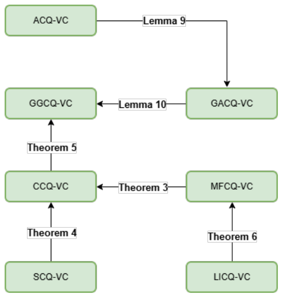
Lemma 9.

For an arbitrary $\mathfrak{q}\in \mathcal{P}$, let ACQ-VC be satisfied at $\mathfrak{q}$. Then GACQ-VC is satisfied at $\mathfrak{q}$.

Lemma 10.

Let $\mathfrak{q}\in \mathcal{P}.$ If GACQ-VC is satisfied at $\mathfrak{q}$, then GGCQ-VC holds at $\mathfrak{q}.$

In the following theorem, we establish that MFCQ-VC is a sufficient condition for the satisfaction of CCQ-VC.

Theorem 3.

Let $\mathfrak{q}$ be an arbitrary element in the feasible set $\mathcal{P}$, such that MFCQ-VC is satisfied at $\mathfrak{q}$. Further, we assume that for every $k\in \mathcal{V}$

$$S_k:=co\left(\bigcup _{\mathfrak{j}\in \mathcal{V},\mathfrak{j}\ne k}\left({\partial }_c{f}_{\mathfrak{j}}^L\left(\mathfrak{q}\right)\cup {\partial }_c{f}_{\mathfrak{j}}^R\left(\mathfrak{q}\right)\right)\right)+pos\left({\mathcal{C}}_{\vartheta }\cup {\mathcal{C}}_{{\mathcal{G}}_2}\cup {\mathcal{C}}_{{\mathcal{H}}_2}\right)+span\left({\mathcal{C}}_{\Theta }\cup {\mathcal{C}}_{{\mathcal{G}}_1}\right)$$

is a closed set. Then CCQ-VC is also satisfied at $\mathfrak{q}.$

Proof. 

Suppose, to the contrary, that CCQ-VC fails to hold at $\mathfrak{q}.$ Then there exists $k\in \mathcal{V}$ for which the system of inequalities stated below

$$\begin{array}{cc}\hfill {\langle {\xi }_{\mathfrak{j}}^L,\nu \rangle }_{\mathfrak{q}}& <0,\mathrm{for}\mathrm{all}{\xi }_{\mathfrak{j}}^L\in {\partial }_c{f}_{\mathfrak{j}}^L\left(\mathfrak{q}\right),\mathrm{for}\mathrm{all}\mathfrak{j}\in \mathcal{V},\mathfrak{j}\ne k,\hfill \\ \hfill {\langle {\xi }_{\mathfrak{j}}^R,\nu \rangle }_{\mathfrak{q}}& <0,\mathrm{for}\mathrm{all}{\xi }_{\mathfrak{j}}^R\in {\partial }_c{f}_{\mathfrak{j}}^R\left(\mathfrak{q}\right),\mathrm{for}\mathrm{all}\mathfrak{j}\in \mathcal{V},\mathfrak{j}\ne k,\hfill \\ \hfill {\langle {\eta }_{\mathfrak{j}}^L,\nu \rangle }_{\mathfrak{q}}& <0,\mathrm{for}\mathrm{all}{\eta }_{\mathfrak{j}}^L\in {\partial }_c{\vartheta }_{\mathfrak{j}}^L\left(\mathfrak{q}\right),\mathrm{for}\mathrm{all}\mathfrak{j}\in \mathcal{N}\left(\mathfrak{q}\right),\hfill \\ \hfill {\langle {\eta }_{\mathfrak{j}}^R,\nu \rangle }_{\mathfrak{q}}& <0,\mathrm{for}\mathrm{all}{\eta }_{\mathfrak{j}}^R\in {\partial }_c{\vartheta }_{\mathfrak{j}}^R\left(\mathfrak{q}\right),\mathrm{for}\mathrm{all}\mathfrak{j}\in \mathcal{N}\left(\mathfrak{q}\right),\hfill \\ \hfill {\langle {\eta }_{\mathfrak{j}}^{\Theta },\nu \rangle }_{\mathfrak{q}}& =0,\mathrm{for}\mathrm{all}{\eta }_{\mathfrak{j}}^{\Theta }\in {\partial }_c{\Theta }_{\mathfrak{j}}\left(\mathfrak{q}\right),\mathrm{for}\mathrm{all}\mathfrak{j}\in {\mathcal{V}}^{\Theta },\hfill \\ \hfill {\langle {\eta }_{\mathfrak{j}}^{\mathcal{G}},\nu \rangle }_{\mathfrak{q}}& =0,\mathrm{for}\mathrm{all}{\eta }_{\mathfrak{j}}^{\mathcal{G}}\in {\partial }_c{\mathcal{G}}_{\mathfrak{j}}\left(\mathfrak{q}\right),\mathrm{for}\mathrm{all}\mathfrak{j}\in {\mathcal{M}}_{0+}\left(\mathfrak{q}\right),\hfill \\ \hfill {\langle {\eta }_{\mathfrak{j}}^{\mathcal{G}},\nu \rangle }_{\mathfrak{q}}& >0,\mathrm{for}\mathrm{all}{\eta }_{\mathfrak{j}}^{\mathcal{G}}\in {\partial }_c{\mathcal{G}}_{\mathfrak{j}}\left(\mathfrak{q}\right),\mathrm{for}\mathrm{all}\mathfrak{j}\in {\mathcal{M}}_{0-}\left(\mathfrak{q}\right)\cup {\mathcal{M}}_{00}\left(\mathfrak{q}\right),\hfill \\ \hfill {\langle {\eta }_{\mathfrak{j}}^{\mathcal{H}},\nu \rangle }_{\mathfrak{q}}& <0,\mathrm{for}\mathrm{all}{\eta }_{\mathfrak{j}}^{\mathcal{H}}\in {\partial }_c{\mathcal{H}}_{\mathfrak{j}}\left(\mathfrak{q}\right),\mathrm{for}\mathrm{all}\mathfrak{j}\in {\mathcal{M}}_{+0}\left(\mathfrak{q}\right)\cup {\mathcal{M}}_{00}\left(\mathfrak{q}\right),\hfill \end{array}$$

does not admit any solution $\nu \in T_{\mathfrak{q}}{\mathbb{H}}^n.$ From Lemma 7 and the given hypotheses, the inclusion below is satisfied:

$$\begin{array}{cc}\hfill 0& \in co\left(\bigcup _{\mathfrak{j}\in \mathcal{V},\mathfrak{j}\ne k}\left({\partial }_c{f}_{\mathfrak{j}}^L\left(\mathfrak{q}\right)\cup {\partial }_c{f}_{\mathfrak{j}}^R\left(\mathfrak{q}\right)\right)\right)+pos\left({\mathcal{C}}_{\vartheta }\cup {\mathcal{C}}_{{\mathcal{G}}_2}\cup {\mathcal{C}}_{{\mathcal{H}}_2}\right)+span\left({\mathcal{C}}_{\Theta }\cup {\mathcal{C}}_{{\mathcal{G}}_1}\right).\hfill \end{array}$$

It follows that there exist ${\xi }_{\mathfrak{j}}^L\in {\partial }_c{f}_{\mathfrak{j}}^L\left(\mathfrak{q}\right)(\mathfrak{j}\in \mathcal{V}),{\xi }_{\mathfrak{j}}^R\in {\partial }_c{f}_{\mathfrak{j}}^R\left(\mathfrak{q}\right)(\mathfrak{j}\in \mathcal{V}),$${\eta }_{\mathfrak{j}}^L\in {\partial }_c{\vartheta }_{\mathfrak{j}}^L\left(\mathfrak{q}\right)(\mathfrak{j}\in \mathcal{N}\left(\mathfrak{q}\right)),{\eta }_{\mathfrak{j}}^R\in {\partial }_c{\vartheta }_{\mathfrak{j}}^R\left(\mathfrak{q}\right)(\mathfrak{j}\in \mathcal{N}\left(\mathfrak{q}\right))$, ${\eta }_{\mathfrak{j}}^{\Theta }\in {\partial }_c{\Theta }_{\mathfrak{j}}\left(\mathfrak{q}\right)(\mathfrak{j}\in {\mathcal{V}}^{\Theta })$, ${\eta }_{\mathfrak{j}}^{\mathcal{G}}\in {\partial }_c{\mathcal{G}}_{\mathfrak{j}}\left(\mathfrak{q}\right)(\mathfrak{j}\in {\mathcal{M}}_{00}\left(\mathfrak{q}\right)\cup {\mathcal{M}}_{0+}\left(\mathfrak{q}\right)\cup {\mathcal{M}}_{0-}\left(\mathfrak{q}\right))$, ${\eta }_{\mathfrak{j}}^{\mathcal{H}}\in {\partial }_c{\mathcal{H}}_{\mathfrak{j}}\left(\mathfrak{q}\right)(\mathfrak{j}\in {\mathcal{M}}_{+0}\left(\mathfrak{q}\right)\cup {\mathcal{M}}_{00}\left(\mathfrak{q}\right))$, such that

$$\begin{array}{cc}\hfill 0& =\sum _{\mathfrak{j}\in \mathcal{V},\mathfrak{j}\ne k}({\lambda }_{\mathfrak{j}}^L{\xi }_{\mathfrak{j}}^L+{\lambda }_{\mathfrak{j}}^R{\xi }_{\mathfrak{j}}^R)+\sum _{\mathfrak{j}\in \mathcal{N}\left(\mathfrak{q}\right)}\left({\sigma }_{\mathfrak{j}}^L{\eta }_{\mathfrak{j}}^L+{\sigma }_{\mathfrak{j}}^R{\eta }_{\mathfrak{j}}^R\right)+\sum _{\mathfrak{j}\in {\mathcal{V}}^{\Theta }}{\sigma }_{\mathfrak{j}}^{\Theta }{\eta }_{\mathfrak{j}}^{\Theta }\hfill \\ & -\sum _{\mathfrak{j}\in {\mathcal{M}}_{00}\left(\mathfrak{q}\right)\cup {\mathcal{M}}_{0+}\left(\mathfrak{q}\right)\cup {\mathcal{M}}_{0-}\left(\mathfrak{q}\right)}{\sigma }_{\mathfrak{j}}^{\mathcal{G}}{\eta }_{\mathfrak{j}}^{\mathcal{G}}+\sum _{\mathfrak{j}\in {\mathcal{M}}_{+0}\left(\mathfrak{q}\right)\cup {\mathcal{M}}_{00}\left(\mathfrak{q}\right)}{\sigma }_{\mathfrak{j}}^{\mathcal{H}}{\eta }_{\mathfrak{j}}^{\mathcal{H}},\hfill \end{array}$$

(11)

with $\sum _{\mathfrak{j}\in \mathcal{V},\mathfrak{j}\ne k}\left({\lambda }_{\mathfrak{j}}^L+{\lambda }_{\mathfrak{j}}^R\right)=1,{\lambda }_{\mathfrak{j}}^L\ge 0,{\lambda }_{\mathfrak{j}}^R\ge 0(\mathfrak{j}\in \mathcal{V},\mathfrak{j}\ne k)$, ${\sigma }_{\mathfrak{j}}^L\ge 0,{\sigma }_{\mathfrak{j}}^R\ge 0(\mathfrak{j}\in \mathcal{N}\left(\mathfrak{q}\right))$, ${\sigma }_{\mathfrak{j}}^{\mathcal{G}}\ge 0(\mathfrak{j}\in {\mathcal{M}}_{0-}\left(\mathfrak{q}\right)\cup {\mathcal{M}}_{00}\left(\mathfrak{q}\right))$, ${\sigma }_{\mathfrak{j}}^{\mathcal{H}}\ge 0(\mathfrak{j}\in {\mathcal{M}}_{+0}\left(\mathfrak{q}\right)\cup {\mathcal{M}}_{00}\left(\mathfrak{q}\right)).$ In light of the imposed hypothesis, MFCQ-VC holds at $\mathfrak{q}$. This implies that the following system of inequalities

$$\begin{array}{cc}\hfill {\langle {\xi }_{\mathfrak{j}}^L,\nu \rangle }_{\mathfrak{q}}& =0,\mathrm{for}\mathrm{all}{\xi }_{\mathfrak{j}}^L\in {\partial }_c{f}_{\mathfrak{j}}^L\left(\mathfrak{q}\right),\mathrm{for}\mathrm{all}\mathfrak{j}\in \mathcal{V},\hfill \\ \hfill {\langle {\xi }_{\mathfrak{j}}^R,\nu \rangle }_{\mathfrak{q}}& =0,\mathrm{for}\mathrm{all}{\xi }_{\mathfrak{j}}^R\in {\partial }_c{f}_{\mathfrak{j}}^R\left(\mathfrak{q}\right),\mathrm{for}\mathrm{all}\mathfrak{j}\in \mathcal{V},\hfill \\ \hfill {\langle {\eta }_{\mathfrak{j}}^L,\nu \rangle }_{\mathfrak{q}}& <0,\mathrm{for}\mathrm{all}{\eta }_{\mathfrak{j}}^L\in {\partial }_c{\vartheta }_{\mathfrak{j}}^L\left(\mathfrak{q}\right),\mathrm{for}\mathrm{all}\mathfrak{j}\in \mathcal{N}\left(\mathfrak{q}\right),\hfill \\ \hfill {\langle {\eta }_{\mathfrak{j}}^R,\nu \rangle }_{\mathfrak{q}}& <0,\mathrm{for}\mathrm{all}{\eta }_{\mathfrak{j}}^R\in {\partial }_c{\vartheta }_{\mathfrak{j}}^R\left(\mathfrak{q}\right),\mathrm{for}\mathrm{all}\mathfrak{j}\in \mathcal{N}\left(\mathfrak{q}\right),\hfill \\ \hfill {\langle {\eta }_{\mathfrak{j}}^{\Theta },\nu \rangle }_{\mathfrak{q}}& =0,\mathrm{for}\mathrm{all}{\eta }_{\mathfrak{j}}^{\Theta }\in {\partial }_c{\Theta }_{\mathfrak{j}}\left(\mathfrak{q}\right),\mathrm{for}\mathrm{all}\mathfrak{j}\in {\mathcal{V}}^{\Theta },\hfill \\ \hfill {\langle {\eta }_{\mathfrak{j}}^{\mathcal{G}},\nu \rangle }_{\mathfrak{q}}& =0,\mathrm{for}\mathrm{all}{\eta }_{\mathfrak{j}}^{\mathcal{G}}\in {\partial }_c{\mathcal{G}}_{\mathfrak{j}}\left(\mathfrak{q}\right),\mathrm{for}\mathrm{all}\mathfrak{j}\in {\mathcal{M}}_{0+}\left(\mathfrak{q}\right),\hfill \\ \hfill {\langle {\eta }_{\mathfrak{j}}^{\mathcal{G}},\nu \rangle }_{\mathfrak{q}}& >0,\mathrm{for}\mathrm{all}{\eta }_{\mathfrak{j}}^{\mathcal{G}}\in {\partial }_c{\mathcal{G}}_{\mathfrak{j}}\left(\mathfrak{q}\right),\mathrm{for}\mathrm{all}\mathfrak{j}\in {\mathcal{M}}_{0-}\left(\mathfrak{q}\right)\cup {\mathcal{M}}_{00}\left(\mathfrak{q}\right),\hfill \\ \hfill {\langle {\eta }_{\mathfrak{j}}^{\mathcal{H}},\nu \rangle }_{\mathfrak{q}}& <0,\mathrm{for}\mathrm{all}{\eta }_{\mathfrak{j}}^{\mathcal{H}}\in {\partial }_c{\mathcal{H}}_{\mathfrak{j}}\left(\mathfrak{q}\right),\mathrm{for}\mathrm{all}\mathfrak{j}\in {\mathcal{M}}_{+0}\left(\mathfrak{q}\right)\cup {\mathcal{M}}_{00}\left(\mathfrak{q}\right),\hfill \end{array}$$

(12)

admits a solution $\nu \in T_{\mathfrak{q}}{\mathbb{H}}^n.$ Therefore, in view of (11) and (12), we have

$$0={〈\sum _{\mathfrak{j}\in \mathcal{N}\left(\mathfrak{q}\right)}({\sigma }_{\mathfrak{j}}^L{\eta }_{\mathfrak{j}}^L+{\sigma }_{\mathfrak{j}}^R{\eta }_{\mathfrak{j}}^R)-\sum _{\mathfrak{j}\in {\mathcal{M}}_{0-}\left(\mathfrak{q}\right)\cup {\mathcal{M}}_{00}\left(\mathfrak{q}\right)}{\sigma }_{\mathfrak{j}}^{\mathcal{G}}{\eta }_{\mathfrak{j}}^{\mathcal{G}}+\sum _{\mathfrak{j}\in {\mathcal{M}}_{+0}\left(\mathfrak{q}\right)\cup {\mathcal{M}}_{00}\left(\mathfrak{q}\right)}{\sigma }_{\mathfrak{j}}^{\mathcal{H}}{\eta }_{\mathfrak{j}}^{\mathcal{H}},\nu 〉}_{\mathfrak{q}}.$$

(13)

Moreover, in light of (12) and (13), we get ${\sigma }_{\mathfrak{j}}^L=0={\sigma }_{\mathfrak{j}}^R(\mathfrak{j}\in \mathcal{N}\left(\mathfrak{q}\right)),{\sigma }_{\mathfrak{j}}^{\mathcal{G}}=0(\mathfrak{j}\in {\mathcal{M}}_{0-}\left(\mathfrak{q}\right)\cup {\mathcal{M}}_{00}\left(\mathfrak{q}\right)),{\sigma }_{\mathfrak{j}}^{\mathcal{H}}=0(\mathfrak{j}\in {\mathcal{M}}_{+0}\left(\mathfrak{q}\right)\cup {\mathcal{M}}_{00}\left(\mathfrak{q}\right)).$ Therefore, from (11) we have

$$0=\sum _{\mathfrak{j}\in \mathcal{V},\mathfrak{j}\ne k}({\lambda }_{\mathfrak{j}}^L{\xi }_{\mathfrak{j}}^L+{\lambda }_{\mathfrak{j}}^R{\xi }_{\mathfrak{j}}^R)+\sum _{\mathfrak{j}\in {\mathcal{V}}^{\Theta }}{\sigma }_{\mathfrak{j}}^{\Theta }{\eta }_{\mathfrak{j}}^{\Theta }-\sum _{\mathfrak{j}\in {\mathcal{M}}_{0+}\left(\mathfrak{q}\right)}{\sigma }_{\mathfrak{j}}^{\mathcal{G}}{\eta }_{\mathfrak{j}}^{\mathcal{G}}.$$

Since MFCQ-VC is satisfied at $\mathfrak{q},$ therefore, ${\lambda }_{\mathfrak{j}}^L=0={\lambda }_{\mathfrak{j}}^R(\mathfrak{j}\in \mathcal{V},\mathfrak{j}\ne k)$, ${\sigma }_{\mathfrak{j}}^{\Theta }=0(\mathfrak{j}\in {\mathcal{V}}^{\Theta }),$${\sigma }_{\mathfrak{j}}^{\mathcal{G}}=0(\mathfrak{j}\in {\mathcal{M}}_{0+}\left(\mathfrak{q}\right)),$ which is a contradiction to the fact that ${\sum }_{\mathfrak{j}\in \mathcal{V},\mathfrak{j}\ne k}\left({\lambda }_{\mathfrak{j}}^L+{\lambda }_{\mathfrak{j}}^R\right)=1$. Therefore, CCQ-VC is satisfied at $\mathfrak{q}.$ □

In the subsequent theorem, we establish that SCQ-VC is sufficient to ensure that CCQ-VC holds.

Theorem 4.

For any $\mathfrak{q}\in \mathcal{P}$, let SCQ-VC be satisfied at $\mathfrak{q}$. Then CCQ-VC is satisfied at $\mathfrak{q}.$

Proof. 

By virtue of the assumed hypothesis, it is evident that SCQ-VC holds at $\mathfrak{q}$. Then for each $k\in \mathcal{V}$, there exists $\mathfrak{p}\in {\mathbb{H}}^n$, satisfying the following:

$$\begin{array}{cc}\hfill f_{\mathfrak{j}}^L\left(\mathfrak{p}\right)& <f_{\mathfrak{j}}^L\left(\mathfrak{q}\right),\mathrm{for}\mathrm{all}\mathfrak{j}\in \mathcal{V},\mathfrak{j}\ne k,\hfill \\ \hfill f_{\mathfrak{j}}^R\left(\mathfrak{p}\right)& <f_{\mathfrak{j}}^R\left(\mathfrak{q}\right),\mathrm{for}\mathrm{all}\mathfrak{j}\in \mathcal{V},\mathfrak{j}\ne k,\hfill \\ \hfill {\vartheta }_{\mathfrak{j}}^L\left(\mathfrak{p}\right)& <0,\mathrm{for}\mathrm{all}\mathfrak{j}\in \mathcal{N}\left(\mathfrak{q}\right),\hfill \\ \hfill {\vartheta }_{\mathfrak{j}}^R\left(\mathfrak{p}\right)& <0,\mathrm{for}\mathrm{all}\mathfrak{j}\in \mathcal{N}\left(\mathfrak{q}\right),\hfill \\ \hfill {\Theta }_{\mathfrak{j}}\left(\mathfrak{p}\right)& =0,\mathrm{for}\mathrm{all}\mathfrak{j}\in {\mathcal{V}}^{\Theta },\hfill \\ \hfill {\mathcal{G}}_{\mathfrak{j}}\left(\mathfrak{p}\right)& =0,\mathrm{for}\mathrm{all}\mathfrak{j}\in {\mathcal{M}}_{0+}\left(\mathfrak{q}\right),\hfill \\ \hfill {\mathcal{G}}_{\mathfrak{j}}\left(\mathfrak{p}\right)& >0,\mathrm{for}\mathrm{all}\mathfrak{j}\in {\mathcal{M}}_{0-}\left(\mathfrak{q}\right)\cup {\mathcal{M}}_{00}\left(\mathfrak{q}\right),\hfill \\ \hfill {\mathcal{H}}_{\mathfrak{j}}\left(\mathfrak{p}\right)& <0,\mathrm{for}\mathrm{all}\mathfrak{j}\in {\mathcal{M}}_{+0}\left(\mathfrak{q}\right)\cup {\mathcal{M}}_{00}\left(\mathfrak{q}\right).\hfill \end{array}$$

(14)

By employing geodesic convexity assumptions on $f_{\mathfrak{j}}^L,f_{\mathfrak{j}}^R(\mathfrak{j}\in \mathcal{V})$, ${\vartheta }_{\mathfrak{j}}^L,{\vartheta }_{\mathfrak{j}}^R(\mathfrak{j}\in \mathcal{N}\left(\mathfrak{q}\right))$, ${\mathcal{H}}_{\mathfrak{j}}(\mathfrak{j}\in {\mathcal{M}}_{+0}\left(\mathfrak{q}\right)\cup {\mathcal{M}}_{00}\left(\mathfrak{q}\right)),-{\mathcal{G}}_{\mathfrak{j}}(\mathfrak{j}\in {\mathcal{M}}_{0-}\left(\mathfrak{q}\right)\cup {\mathcal{M}}_{00}\left(\mathfrak{q}\right))$, and geodesic affine assumptions on ${\mathcal{G}}_{\mathfrak{j}}(\mathfrak{j}\in {\mathcal{M}}_{0+}\left(\mathfrak{q}\right))$, ${\Theta }_{\mathfrak{j}}(\mathfrak{j}\in {\mathcal{V}}^{\Theta })$ in (14), it follows that

$$\begin{array}{cc}\hfill {\langle {\xi }_{\mathfrak{j}}^L,{exp}_{\mathfrak{q}}^{-1}\left(\mathfrak{p}\right)\rangle }_{\mathfrak{q}}& <0,\mathrm{for}\mathrm{all}{\xi }_{\mathfrak{j}}^L\in {\partial }_c{f}_{\mathfrak{j}}^L\left(\mathfrak{q}\right),\mathrm{for}\mathrm{all}\mathfrak{j}\in \mathcal{V},\mathfrak{j}\ne k,\hfill \\ \hfill {\langle {\xi }_{\mathfrak{j}}^R,{exp}_{\mathfrak{q}}^{-1}\left(\mathfrak{p}\right)\rangle }_{\mathfrak{q}}& <0,\mathrm{for}\mathrm{all}{\xi }_{\mathfrak{j}}^R\in {\partial }_c{f}_{\mathfrak{j}}^R\left(\mathfrak{q}\right),\mathrm{for}\mathrm{all}\mathfrak{j}\in \mathcal{V},\mathfrak{j}\ne k,\hfill \\ \hfill {\langle {\eta }_{\mathfrak{j}}^L,{exp}_{\mathfrak{q}}^{-1}\left(\mathfrak{p}\right)\rangle }_{\mathfrak{q}}& <0,\mathrm{for}\mathrm{all}{\eta }_{\mathfrak{j}}^L\in {\partial }_c{\vartheta }_{\mathfrak{j}}^L\left(\mathfrak{q}\right),\mathrm{for}\mathrm{all}\mathfrak{j}\in \mathcal{N}\left(\mathfrak{q}\right),\hfill \\ \hfill {\langle {\eta }_{\mathfrak{j}}^R,{exp}_{\mathfrak{q}}^{-1}\left(\mathfrak{p}\right)\rangle }_{\mathfrak{q}}& <0,\mathrm{for}\mathrm{all}{\eta }_{\mathfrak{j}}^R\in {\partial }_c{\vartheta }_{\mathfrak{j}}^R\left(\mathfrak{q}\right),\mathrm{for}\mathrm{all}\mathfrak{j}\in \mathcal{N}\left(\mathfrak{q}\right),\hfill \\ \hfill {\langle {\eta }_{\mathfrak{j}}^{\Theta },{exp}_{\mathfrak{q}}^{-1}\left(\mathfrak{p}\right)\rangle }_{\mathfrak{q}}& =0,\mathrm{for}\mathrm{all}{\eta }_{\mathfrak{j}}^{\Theta }\in {\partial }_c{\Theta }_{\mathfrak{j}}\left(\mathfrak{q}\right),\mathrm{for}\mathrm{all}\mathfrak{j}\in {\mathcal{V}}^{\Theta },\hfill \\ \hfill {\langle {\eta }_{\mathfrak{j}}^{\mathcal{G}},{exp}_{\mathfrak{q}}^{-1}\left(\mathfrak{p}\right)\rangle }_{\mathfrak{q}}& =0,\mathrm{for}\mathrm{all}{\eta }_{\mathfrak{j}}^{\mathcal{G}}\in {\partial }_c{\mathcal{G}}_{\mathfrak{j}}\left(\mathfrak{q}\right),\mathrm{for}\mathrm{all}\mathfrak{j}\in {\mathcal{M}}_{0+}\left(\mathfrak{q}\right),\hfill \\ \hfill {\langle {\eta }_{\mathfrak{j}}^{\mathcal{G}},{exp}_{\mathfrak{q}}^{-1}\left(\mathfrak{p}\right)\rangle }_{\mathfrak{q}}& >0,\mathrm{for}\mathrm{all}{\eta }_{\mathfrak{j}}^{\mathcal{G}}\in {\partial }_c{\mathcal{G}}_{\mathfrak{j}}\left(\mathfrak{q}\right),\mathrm{for}\mathrm{all}\mathfrak{j}\in {\mathcal{M}}_{0-}\left(\mathfrak{q}\right)\cup {\mathcal{M}}_{00}\left(\mathfrak{q}\right),\hfill \\ \hfill {\langle {\eta }_{\mathfrak{j}}^{\mathcal{H}},{exp}_{\mathfrak{q}}^{-1}\left(\mathfrak{p}\right)\rangle }_{\mathfrak{q}}& <0,\mathrm{for}\mathrm{all}{\eta }_{\mathfrak{j}}^{\mathcal{H}}\in {\partial }_c{\mathcal{H}}_{\mathfrak{j}}\left(\mathfrak{q}\right),\mathrm{for}\mathrm{all}\mathfrak{j}\in {\mathcal{M}}_{+0}\left(\mathfrak{q}\right)\cup {\mathcal{M}}_{00}\left(\mathfrak{q}\right).\hfill \end{array}$$

Therefore, (10) is satisfied at $\mathfrak{q}$ by setting $\nu ={exp}_{\mathfrak{q}}^{-1}\left(\mathfrak{p}\right)\in T_{\mathfrak{q}}{\mathbb{H}}^n.$ □

In the subsequent theorem, we establish that CCQ-VC is a sufficient condition for guaranteeing that GGCQ-VC holds.

Theorem 5.

For any arbitrary element $\mathfrak{q}\in \mathcal{P}$, let CCQ-VC be satisfied at $\mathfrak{q}.$ Then GGCQ-VC is satisfied at $\mathfrak{q}.$

Proof. 

From the given hypothesis, there exists $\widehat{w}\in T_{\mathfrak{q}}{\mathbb{H}}^n$, such that the system of inequalities in (10) is satisfied for $k=1.$ Equivalently,

$$\begin{array}{cc}\hfill {\langle {\xi }_{\mathfrak{j}}^L,\widehat{w}\rangle }_{\mathfrak{q}}& <0,\mathrm{for}\mathrm{all}{\xi }_{\mathfrak{j}}^L\in {\partial }_c{f}_{\mathfrak{j}}^L\left(\mathfrak{q}\right),\mathrm{for}\mathrm{all}\mathfrak{j}\in \mathcal{V},\mathfrak{j}\ne 1,\hfill \\ \hfill {\langle {\xi }_{\mathfrak{j}}^R,\widehat{w}\rangle }_{\mathfrak{q}}& <0,\mathrm{for}\mathrm{all}{\xi }_{\mathfrak{j}}^R\in {\partial }_c{f}_{\mathfrak{j}}^R\left(\mathfrak{q}\right),\mathrm{for}\mathrm{all}\mathfrak{j}\in \mathcal{V},\mathfrak{j}\ne 1,\hfill \\ \hfill {\langle {\eta }_{\mathfrak{j}}^L,\widehat{w}\rangle }_{\mathfrak{q}}& <0,\mathrm{for}\mathrm{all}{\eta }_{\mathfrak{j}}^L\in {\partial }_c{\vartheta }_{\mathfrak{j}}^L\left(\mathfrak{q}\right),\mathrm{for}\mathrm{all}\mathfrak{j}\in \mathcal{N}\left(\mathfrak{q}\right),\hfill \\ \hfill {\langle {\eta }_{\mathfrak{j}}^R,\widehat{w}\rangle }_{\mathfrak{q}}& <0,\mathrm{for}\mathrm{all}{\eta }_{\mathfrak{j}}^R\in {\partial }_c{\vartheta }_{\mathfrak{j}}^R\left(\mathfrak{q}\right),\mathrm{for}\mathrm{all}\mathfrak{j}\in \mathcal{N}\left(\mathfrak{q}\right),\hfill \\ \hfill {\langle {\eta }_{\mathfrak{j}}^{\Theta },\widehat{w}\rangle }_{\mathfrak{q}}& =0,\mathrm{for}\mathrm{all}{\eta }_{\mathfrak{j}}^{\Theta }\in {\partial }_c{\Theta }_{\mathfrak{j}}\left(\mathfrak{q}\right),\mathrm{for}\mathrm{all}\mathfrak{j}\in {\mathcal{V}}^{\Theta },\hfill \\ \hfill {\langle {\eta }_{\mathfrak{j}}^{\mathcal{G}},\widehat{w}\rangle }_{\mathfrak{q}}& =0,\mathrm{for}\mathrm{all}{\eta }_{\mathfrak{j}}^{\mathcal{G}}\in {\partial }_c{\mathcal{G}}_{\mathfrak{j}}\left(\mathfrak{q}\right),\mathrm{for}\mathrm{all}\mathfrak{j}\in {\mathcal{M}}_{0+}\left(\mathfrak{q}\right),\hfill \\ \hfill {\langle {\eta }_{\mathfrak{j}}^{\mathcal{G}},\widehat{w}\rangle }_{\mathfrak{q}}& >0,\mathrm{for}\mathrm{all}{\eta }_{\mathfrak{j}}^{\mathcal{G}}\in {\partial }_c{\mathcal{G}}_{\mathfrak{j}}\left(\mathfrak{q}\right),\mathrm{for}\mathrm{all}\mathfrak{j}\in {\mathcal{M}}_{0-}\left(\mathfrak{q}\right)\cup {\mathcal{M}}_{00}\left(\mathfrak{q}\right),\hfill \\ \hfill {\langle {\eta }_{\mathfrak{j}}^{\mathcal{H}},\widehat{w}\rangle }_{\mathfrak{q}}& <0,\mathrm{for}\mathrm{all}{\eta }_{\mathfrak{j}}^{\mathcal{H}}\in {\partial }_c{\mathcal{H}}_{\mathfrak{j}}\left(\mathfrak{q}\right),\mathrm{for}\mathrm{all}\mathfrak{j}\in {\mathcal{M}}_{+0}\left(\mathfrak{q}\right)\cup {\mathcal{M}}_{00}\left(\mathfrak{q}\right).\hfill \end{array}$$

(15)

Now, we need to prove that

$$L^{VC}(\mathfrak{q};X)\subseteq \bigcap _{k\in \mathcal{V}}clco\mathcal{C}(\mathfrak{q},X^k).$$

For this, let us assume that $\nu \in L^{VC}(\mathfrak{q};X)$. It follows that

$$\begin{array}{cc}\hfill & {\langle {\xi }_{\mathfrak{j}}^L,\nu \rangle }_{\mathfrak{q}}\le 0,\mathrm{for}\mathrm{all}{\xi }_{\mathfrak{j}}^L\in {\partial }_c{f}_{\mathfrak{j}}^L\left(\mathfrak{q}\right),\mathrm{for}\mathrm{all}\mathfrak{j}\in \mathcal{V},\hfill \\ \hfill & {\langle {\xi }_{\mathfrak{j}}^R,\nu \rangle }_{\mathfrak{q}}\le 0,\mathrm{for}\mathrm{all}{\xi }_{\mathfrak{j}}^R\in {\partial }_c{f}_{\mathfrak{j}}^R\left(\mathfrak{q}\right),\mathrm{for}\mathrm{all}\mathfrak{j}\in \mathcal{V},\hfill \\ \hfill & {\langle {\eta }_{\mathfrak{j}}^L,\nu \rangle }_{\mathfrak{q}}\le 0,\mathrm{for}\mathrm{all}{\eta }_{\mathfrak{j}}^L\in {\partial }_c{\vartheta }_{\mathfrak{j}}^L\left(\mathfrak{q}\right),\mathrm{for}\mathrm{all}\mathfrak{j}\in \mathcal{N}\left(\mathfrak{q}\right),\hfill \\ \hfill & {\langle {\eta }_{\mathfrak{j}}^R,\nu \rangle }_{\mathfrak{q}}\le 0,\mathrm{for}\mathrm{all}{\eta }_{\mathfrak{j}}^R\in {\partial }_c{\vartheta }_{\mathfrak{j}}^R\left(\mathfrak{q}\right),\mathrm{for}\mathrm{all}\mathfrak{j}\in \mathcal{N}\left(\mathfrak{q}\right),\hfill \\ \hfill & {\langle {\eta }_{\mathfrak{j}}^{\Theta },\nu \rangle }_{\mathfrak{q}}=0,\mathrm{for}\mathrm{all}{\eta }_{\mathfrak{j}}^{\Theta }\in {\partial }_c{\Theta }_{\mathfrak{j}}\left(\mathfrak{q}\right)\mathrm{for}\mathrm{all}\mathfrak{j}\in {\mathcal{V}}^{\Theta },\hfill \\ \hfill & {\langle {\eta }_{\mathfrak{j}}^{\mathcal{G}},\nu \rangle }_{\mathfrak{q}}=0,\mathrm{for}\mathrm{all}{\eta }_{\mathfrak{j}}^{\mathcal{G}}\in {\partial }_c{\mathcal{G}}_{\mathfrak{j}}\left(\mathfrak{q}\right),\mathrm{for}\mathrm{all}\mathfrak{j}\in {\mathcal{M}}_{0+}\left(\mathfrak{q}\right),\hfill \\ \hfill & {\langle {\eta }_{\mathfrak{j}}^{\mathcal{G}},\nu \rangle }_{\mathfrak{q}}\ge 0,\mathrm{for}\mathrm{all}{\eta }_{\mathfrak{j}}^{\mathcal{G}}\in {\partial }_c{\mathcal{G}}_{\mathfrak{j}}\left(\mathfrak{q}\right),\mathrm{for}\mathrm{all}\mathfrak{j}\in {\mathcal{M}}_{0-}\left(\mathfrak{q}\right)\cup {\mathcal{M}}_{00}\left(\mathfrak{q}\right),\hfill \\ \hfill & {\langle {\eta }_{\mathfrak{j}}^{\mathcal{H}},\nu \rangle }_{\mathfrak{q}}\le 0,\mathrm{for}\mathrm{all}{\eta }_{\mathfrak{j}}^{\mathcal{H}}\in {\partial }_c{\mathcal{H}}_{\mathfrak{j}}\left(\mathfrak{q}\right),\mathrm{for}\mathrm{all}\mathfrak{j}\in {\mathcal{M}}_{+0}\left(\mathfrak{q}\right)\cup {\mathcal{M}}_{00}\left(\mathfrak{q}\right).\hfill \end{array}$$

(16)

Let us consider a sequence ${\left\{t_m\right\}}_{m=1}^{\infty }\subseteq \mathbb{R}$, such that $t_m\downarrow 0$ as $m\to \infty .$ Further, we define a sequence ${\left\{{\nu }_m\right\}}_{m=1}^{\infty }\subseteq T_{\mathfrak{q}}{\mathbb{H}}^n$ as follows:

$${\nu }_m:=\nu +t_m\widehat{w},\mathrm{for}\mathrm{all}m\in \mathbb{N}.$$

(17)

Notably, ${\nu }_m\to \nu$ as $m\to \infty .$ In view of (15), (16), and (17) we have

$$\begin{array}{cc}\hfill {\langle {\xi }_{\mathfrak{j}}^L,{\nu }_m\rangle }_{\mathfrak{q}}& <0,\mathrm{for}\mathrm{all}{\xi }_{\mathfrak{j}}^L\in {\partial }_c{f}_{\mathfrak{j}}^L\left(\mathfrak{q}\right),\mathrm{for}\mathrm{all}\mathfrak{j}\in \mathcal{V},\mathfrak{j}\ne 1,\hfill \\ \hfill {\langle {\xi }_{\mathfrak{j}}^R,{\nu }_m\rangle }_{\mathfrak{q}}& <0,\mathrm{for}\mathrm{all}{\xi }_{\mathfrak{j}}^R\in {\partial }_c{f}_{\mathfrak{j}}^R\left(\mathfrak{q}\right),\mathrm{for}\mathrm{all}\mathfrak{j}\in \mathcal{V},\mathfrak{j}\ne 1,\hfill \\ \hfill {\langle {\eta }_{\mathfrak{j}}^L,{\nu }_m\rangle }_{\mathfrak{q}}& <0,\mathrm{for}\mathrm{all}{\eta }_{\mathfrak{j}}^L\in {\partial }_c{\vartheta }_{\mathfrak{j}}^L\left(\mathfrak{q}\right),\mathrm{for}\mathrm{all}\mathfrak{j}\in \mathcal{N}\left(\mathfrak{q}\right),\hfill \\ \hfill {\langle {\eta }_{\mathfrak{j}}^R,{\nu }_m\rangle }_{\mathfrak{q}}& <0,\mathrm{for}\mathrm{all}{\eta }_{\mathfrak{j}}^R\in {\partial }_c{\vartheta }_{\mathfrak{j}}^R\left(\mathfrak{q}\right),\mathrm{for}\mathrm{all}\mathfrak{j}\in \mathcal{N}\left(\mathfrak{q}\right),\hfill \\ \hfill {\langle {\eta }_{\mathfrak{j}}^{\Theta },{\nu }_m\rangle }_{\mathfrak{q}}& =0,\mathrm{for}\mathrm{all}{\eta }_{\mathfrak{j}}^{\Theta }\in {\partial }_c{\Theta }_{\mathfrak{j}}\left(\mathfrak{q}\right),\mathrm{for}\mathrm{all}\mathfrak{j}\in {\mathcal{V}}^{\Theta },\hfill \\ \hfill {\langle {\eta }_{\mathfrak{j}}^{\mathcal{G}},{\nu }_m\rangle }_{\mathfrak{q}}& =0,\mathrm{for}\mathrm{all}{\eta }_{\mathfrak{j}}^{\mathcal{G}}\in {\partial }_c{\mathcal{G}}_{\mathfrak{j}}\left(\mathfrak{q}\right),\mathrm{for}\mathrm{all}\mathfrak{j}\in {\mathcal{M}}_{0+}\left(\mathfrak{q}\right),\hfill \\ \hfill {\langle {\eta }_{\mathfrak{j}}^{\mathcal{G}},{\nu }_m\rangle }_{\mathfrak{q}}& >0,\mathrm{for}\mathrm{all}{\eta }_{\mathfrak{j}}^{\mathcal{G}}\in {\partial }_c{\mathcal{G}}_{\mathfrak{j}}\left(\mathfrak{q}\right),\mathrm{for}\mathrm{all}\mathfrak{j}\in {\mathcal{M}}_{0-}\left(\mathfrak{q}\right)\cup {\mathcal{M}}_{00}\left(\mathfrak{q}\right),\hfill \\ \hfill {\langle {\eta }_{\mathfrak{j}}^{\mathcal{H}},{\nu }_m\rangle }_{\mathfrak{q}}& <0,\mathrm{for}\mathrm{all}{\eta }_{\mathfrak{j}}^{\mathcal{H}}\in {\partial }_c{\mathcal{H}}_{\mathfrak{j}}\left(\mathfrak{q}\right),\mathrm{for}\mathrm{all}\mathfrak{j}\in {\mathcal{M}}_{+0}\left(\mathfrak{q}\right)\cup {\mathcal{M}}_{00}\left(\mathfrak{q}\right).\hfill \end{array}$$

Now, corresponding to every element of the sequence ${\left\{{\nu }_m\right\}}_{m=1}^{\infty },$ we consider a sequence ${\left\{{\tau }_{m_l}\right\}}_{l=1}^{\infty }\subseteq \mathbb{R}$, such that ${\tau }_{m_l}\downarrow 0$ as $l\to \infty .$ Consequently, we may construct a sequence ${\left\{{\mathfrak{q}}_{m_l}\right\}}_{l=1}^{\infty }$ as follows:

$${\mathfrak{q}}_{m_l}:={exp}_{\mathfrak{q}}\left({\tau }_{m_l}{\nu }_m\right),\mathrm{for}\mathrm{all}l\in \mathbb{N}.$$

Notably, ${\mathfrak{q}}_{m_l}\to \mathfrak{q}$ as $l\to \infty .$ By invoking Theorem 1 for every $m_l\in \mathbb{N}$, there exist some ${\rho }_{m_l}\in (0,1)$, $u_{m_l}=\Omega \left({\rho }_{m_l}\right)$, and ${\xi }_{\mathfrak{j}}^{m_l}\in {\partial }_c{f}_{\mathfrak{j}}^L\left(u_{m_l}\right)$, such that

$$f_{\mathfrak{j}}^L\left({\mathfrak{q}}_{m_l}\right)-f_{\mathfrak{j}}^L\left(\mathfrak{q}\right)={\langle {\xi }_{\mathfrak{j}}^{m_l},{\Omega }^{\prime }\left({\rho }_{m_l}\right)\rangle }_{u_{m_l}},\mathrm{for}\mathrm{all}\mathfrak{j}\in \mathcal{V}\setminus \left\{1\right\},$$

(18)

where $\Omega \left({\rho }_{m_l}\right):={exp}_{\mathfrak{q}}\left({\rho }_{m_l}{exp}_{\mathfrak{q}}^{-1}\left({\mathfrak{q}}_{m_l}\right)\right).$ Notably, ${\rho }_{m_l}\to 0$ and $u_{m_l}\to \mathfrak{q}$ as $l\to \infty .$ Then in view of Lemma 1, we infer that there exists a subsequence ${\left\{{\xi }_{\mathfrak{j}}^{m_{l_{\mathfrak{i}}}}\right\}}_{\mathfrak{i}=1}^{\infty }$ of ${\left\{{\xi }_{\mathfrak{j}}^{m_l}\right\}}_{l=1}^{\infty }$ such that ${\xi }_{\mathfrak{j}}^{m_{l_{\mathfrak{i}}}}\to {\xi }_{\mathfrak{j}}\in {\partial }_c{f}_{\mathfrak{j}}^L\left(\mathfrak{q}\right)(\mathfrak{j}\in \mathcal{V}\setminus \left\{1\right\})$ as $\mathfrak{i}\to \infty$. In the light of (18), it follows that for every $\mathfrak{i}\in \mathbb{N}$ we have:

$$f_{\mathfrak{j}}^L\left({\mathfrak{q}}_{m_{l_{\mathfrak{i}}}}\right)-f_{\mathfrak{j}}^L\left(\mathfrak{q}\right)={\tau }_{m_{l_{\mathfrak{i}}}}\langle {\xi }_{\mathfrak{j}}^{m_{l_{\mathfrak{i}}}},{\nu }_m\rangle ,\mathrm{for}\mathrm{all}\mathfrak{j}\in \mathcal{V}\setminus \left\{1\right\}.$$

(19)

Since ${\langle {\xi }_{\mathfrak{j}}^{m_{l_{\mathfrak{i}}}},{\nu }_m\rangle }_{\mathfrak{q}}\to {\langle {\xi }_{\mathfrak{j}},{\nu }_m\rangle }_{\mathfrak{q}}<0$ as $\mathfrak{i}\to \infty$, it follows from (19) that

$$\underset{\mathfrak{i}\to \infty }{lim\; sup}\left(f_{\mathfrak{j}}^L\left({\mathfrak{q}}_{m_{l_{\mathfrak{i}}}}\right)-f_{\mathfrak{j}}^L\left(\mathfrak{q}\right)\right)<0,\mathrm{for}\mathrm{all}\mathfrak{j}\in \mathcal{V}\setminus \left\{1\right\}.$$

This implies that there exists a natural number $K_1$ such that

$$f_{\mathfrak{j}}^L\left({\mathfrak{q}}_{m_{l_{\mathfrak{i}}}}\right)<f_{\mathfrak{j}}^L\left(\mathfrak{q}\right),\mathrm{for}\mathrm{all}\mathfrak{i}\ge K_1,\mathrm{for}\mathrm{all}\mathfrak{j}\in \mathcal{V}\setminus \left\{1\right\}.$$

(20)

Following the similar steps, there exist $K_2,K_3\in \mathbb{N}$ such that we have:

$$\begin{array}{cc}\hfill f_{\mathfrak{j}}^R\left({\mathfrak{q}}_{m_{l_{\mathfrak{i}}}}\right)& <f_{\mathfrak{j}}^R\left(\mathfrak{q}\right),\mathrm{for}\mathrm{all}\mathfrak{i}\ge K_2,\mathrm{for}\mathrm{all}\mathfrak{j}\in \mathcal{V}\setminus \left\{1\right\},\hfill \\ \hfill {\vartheta }_{\mathfrak{j}}\left({\mathfrak{q}}_{m_{l_{\mathfrak{i}}}}\right)& {⪯}_{LR}[0,0],\mathrm{for}\mathrm{all}\mathfrak{i}\ge K_3,\mathrm{for}\mathrm{all}\mathfrak{j}\in \mathcal{N}\left(\mathfrak{q}\right).\hfill \end{array}$$

(21)

For every $\mathfrak{j}\in \mathcal{N}\setminus \mathcal{N}\left(\mathfrak{q}\right)$, by employing the continuity property of ${\vartheta }_{\mathfrak{j}}^L$ and ${\vartheta }_{\mathfrak{j}}^R$, there exist $K_4\in \mathbb{N}$ such that

$$\begin{array}{c}\hfill {\vartheta }_{\mathfrak{j}}\left({\mathfrak{q}}_{m_{l_{\mathfrak{i}}}}\right){\prec }_{LR}^s[0,0],\mathrm{for}\mathrm{all}\mathfrak{i}\ge K_4.\end{array}$$

(22)

Proceeding analogously one can show that

$$\begin{array}{cc}\hfill {\Theta }_{\mathfrak{j}}\left({\mathfrak{q}}_{m_{l_{\mathfrak{i}}}}\right)& =0,\mathrm{for}\mathrm{all}\mathfrak{i}\ge K_5\mathrm{for}\mathrm{all}\mathfrak{j}\in {\mathcal{V}}^{\Theta },\hfill \\ \hfill {\mathcal{G}}_{\mathfrak{j}}\left({\mathfrak{q}}_{m_{l_{\mathfrak{i}}}}\right)& =0,\mathrm{for}\mathrm{all}\mathfrak{i}\ge K_6\mathrm{for}\mathrm{all}\mathfrak{j}\in {\mathcal{M}}_{0+}\left(\mathfrak{q}\right),\hfill \\ \hfill {\mathcal{G}}_{\mathfrak{j}}\left({\mathfrak{q}}_{m_{l_{\mathfrak{i}}}}\right)& \ge 0,\mathrm{for}\mathrm{all}\mathfrak{i}\ge K_7\mathrm{for}\mathrm{all}\mathfrak{j}\in {\mathcal{M}}_{0-}\left(\mathfrak{q}\right)\cup {\mathcal{M}}_{00}\left(\mathfrak{q}\right)\cup {\mathcal{M}}_{+0}\left(\mathfrak{q}\right)\cup {\mathcal{M}}_{+-}\left(\mathfrak{q}\right),\hfill \\ \hfill {\mathcal{H}}_{\mathfrak{j}}\left({\mathfrak{q}}_{m_{l_{\mathfrak{i}}}}\right)& \le 0,\mathrm{for}\mathrm{all}\mathfrak{i}\ge K_8\mathrm{for}\mathrm{all}\mathfrak{j}\in {\mathcal{M}}_{+0}\left(\mathfrak{q}\right)\cup {\mathcal{M}}_{00}\left(\mathfrak{q}\right)\cup {\mathcal{M}}_{0-}\left(\mathfrak{q}\right)\cup {\mathcal{M}}_{+-}\left(\mathfrak{q}\right).\hfill \end{array}$$

(23)

From (20), (21), (22), and (23), and by choosing $K=max\{K_1,K_2,\dots ,K_8\}$ it follows that

$${\mathfrak{q}}_{m_{l_{\mathfrak{i}}}}={exp}_{\mathfrak{q}}\left({\tau }_{m_{l_{\mathfrak{i}}}}{\nu }_m\right)\in X^1,\mathrm{for}\mathrm{all}\mathfrak{i}\ge K.$$

There is no loss of generality in assuming that ${\mathfrak{q}}_{m_{l_{\mathfrak{i}}}}\in X^1$ for all indices $\mathfrak{i}$. This implies that

$$\nu \in \mathcal{C}(\mathfrak{q},X^1).$$

Using the same argument, it follows that $\nu \in \mathcal{C}(\mathfrak{q},X^k)$ for every $k\in \mathcal{V}$. Then the following inclusion holds:

$$\nu \in \bigcap _{k\in \mathcal{V}}\mathcal{C}(\mathfrak{q},X^k)\subseteq \bigcap _{k\in \mathcal{V}}clco\mathcal{C}(\mathfrak{q},X^k).$$

Therefore, we have

$$L^{VC}(\mathfrak{q};X)\subseteq \bigcap _{k\in \mathcal{V}}clco\mathcal{C}(\mathfrak{q},X^k).$$

(24)

This completes the proof. □

Remark 3.

(i)

Let ${\mathbb{H}}^n={\mathbb{R}}^n$, $f_{\mathfrak{j}}^L\left(\mathfrak{q}\right)=f_{\mathfrak{j}}^R\left(\mathfrak{q}\right)=f_{\mathfrak{j}}\left(\mathfrak{q}\right)(\mathfrak{j}\in \mathcal{V})$, ${\vartheta }_{\mathfrak{j}}^L\left(\mathfrak{q}\right)={\vartheta }_{\mathfrak{j}}^R\left(\mathfrak{q}\right)={\vartheta }_{\mathfrak{j}}\left(\mathfrak{q}\right)(\mathfrak{j}\in \mathcal{N})$, for all $\mathfrak{q}\in {\mathbb{H}}^n$. If $\mathcal{M}=\varnothing ={\mathcal{V}}^{\Theta }$, $f_{\mathfrak{j}}(\mathfrak{j}\in \mathcal{V})$, ${\vartheta }_{\mathfrak{j}}(\mathfrak{j}\in \mathcal{N})$, are continuously differentiable functions on ${\mathbb{H}}^n$, then Theorems 3, 4, and 5 reduce to Lemmas 4.3, 4.4, and 4.5, respectively, as derived by Maeda [45].

(ii)

Theorem 5 generalizes Theorem 6.5 established by Mishra et al. [6] from the Euclidean space setting to the framework of Hadamard manifolds, as well as from smooth multiobjective MPVC to a nonsmooth multiobjective MPVC involving interval-valued objective functions and interval-valued inequality constraint functions.

(iii)

If for every $\mathfrak{q}\in {\mathbb{H}}^n$, $f_{\mathfrak{j}}^L\left(\mathfrak{q}\right)=f_{\mathfrak{j}}^R\left(\mathfrak{q}\right)(\mathfrak{j}\in \mathcal{V})$, ${\vartheta }_{\mathfrak{j}}^L\left(\mathfrak{q}\right)={\vartheta }_{\mathfrak{j}}^R\left(\mathfrak{q}\right)(\mathfrak{j}\in \mathcal{N})$, ${\mathcal{V}}^{\Theta }=\varnothing =\mathcal{M}$, and $f_{\mathfrak{j}}(\mathfrak{j}\in \mathcal{V})$, ${\vartheta }_{\mathfrak{j}}(\mathfrak{j}\in \mathcal{N})$ are continuously differentiable functions, then Theorems 3, 4, and 5 reduce to Theorems 4.3, 4.4, and 4.5, respectively, as deduced by Ghosh et al. [36].

In the following theorem, we establish that if LICQ-VC is satisfied at some feasible element of NIMPPVC, then MFCQ-VC is satisfied at the same point.

Theorem 6.

Let $\mathfrak{q}\in \mathcal{P}$, such that

$$co\left(\bigcup _{\mathfrak{j}\in \mathcal{V}}\left({\partial }_c{f}_{\mathfrak{j}}^L\left(\mathfrak{q}\right)\cup {\partial }_c{f}_{\mathfrak{j}}^R\left(\mathfrak{q}\right)\right)\right)+pos\left({\mathcal{C}}_{\vartheta }\cup {\mathcal{C}}_{{\mathcal{G}}_2}\cup {\mathcal{C}}_{{\mathcal{H}}_2}\right)+span\left({\mathcal{C}}_{\Theta }\cup {\mathcal{C}}_{{\mathcal{G}}_1}\right)$$

is a closed set. If LICQ-VC holds at $\mathfrak{q}$, then MFCQ-VC is satisfied at $\mathfrak{q}$.

Proof. 

Suppose, to the contrary, that there is no $\nu \in T_{\mathfrak{q}}{\mathbb{H}}^n$, satisfying the system of inequalities given below:

$$\begin{array}{cc}\hfill {\langle {\xi }_{\mathfrak{j}}^L,\nu \rangle }_{\mathfrak{q}}& <0,\mathrm{for}\mathrm{all}{\xi }_{\mathfrak{j}}^L\in {\partial }_c{f}_{\mathfrak{j}}^L\left(\mathfrak{q}\right),\mathrm{for}\mathrm{all}\mathfrak{j}\in \mathcal{V},\hfill \\ \hfill {\langle {\xi }_{\mathfrak{j}}^R,\nu \rangle }_{\mathfrak{q}}& <0,\mathrm{for}\mathrm{all}{\xi }_{\mathfrak{j}}^R\in {\partial }_c{f}_{\mathfrak{j}}^R\left(\mathfrak{q}\right),\mathrm{for}\mathrm{all}\mathfrak{j}\in \mathcal{V},\hfill \\ \hfill {\langle {\eta }_{\mathfrak{j}}^L,\nu \rangle }_{\mathfrak{q}}& <0,\mathrm{for}\mathrm{all}{\eta }_{\mathfrak{j}}^L\in {\partial }_c{\vartheta }_{\mathfrak{j}}^L\left(\mathfrak{q}\right),\mathrm{for}\mathrm{all}\mathfrak{j}\in \mathcal{N}\left(\mathfrak{q}\right),\hfill \\ \hfill {\langle {\eta }_{\mathfrak{j}}^R,\nu \rangle }_{\mathfrak{q}}& <0,\mathrm{for}\mathrm{all}{\eta }_{\mathfrak{j}}^R\in {\partial }_c{\vartheta }_{\mathfrak{j}}^R\left(\mathfrak{q}\right),\mathrm{for}\mathrm{all}\mathfrak{j}\in \mathcal{N}\left(\mathfrak{q}\right),\hfill \\ \hfill {\langle {\eta }_{\mathfrak{j}}^{\Theta },\nu \rangle }_{\mathfrak{q}}& =0,\mathrm{for}\mathrm{all}{\eta }_{\mathfrak{j}}^{\Theta }\in {\partial }_c{\Theta }_{\mathfrak{j}}\left(\mathfrak{q}\right),\mathrm{for}\mathrm{all}\mathfrak{j}\in {\mathcal{V}}^{\Theta },\hfill \\ \hfill {\langle {\eta }_{\mathfrak{j}}^{\mathcal{G}},\nu \rangle }_{\mathfrak{q}}& =0,\mathrm{for}\mathrm{all}{\eta }_{\mathfrak{j}}^{\mathcal{G}}\in {\partial }_c{\mathcal{G}}_{\mathfrak{j}}\left(\mathfrak{q}\right),\mathrm{for}\mathrm{all}\mathfrak{j}\in {\mathcal{M}}_{0+}\left(\mathfrak{q}\right),\hfill \\ \hfill {\langle {\eta }_{\mathfrak{j}}^{\mathcal{G}},\nu \rangle }_{\mathfrak{q}}& >0,\mathrm{for}\mathrm{all}{\eta }_{\mathfrak{j}}^{\mathcal{G}}\in {\partial }_c{\mathcal{G}}_{\mathfrak{j}}\left(\mathfrak{q}\right),\mathrm{for}\mathrm{all}\mathfrak{j}\in {\mathcal{M}}_{0-}\left(\mathfrak{q}\right)\cup {\mathcal{M}}_{00}\left(\mathfrak{q}\right),\hfill \\ \hfill {\langle {\eta }_{\mathfrak{j}}^{\mathcal{H}},\nu \rangle }_{\mathfrak{q}}& <0,\mathrm{for}\mathrm{all}{\eta }_{\mathfrak{j}}^{\mathcal{H}}\in {\partial }_c{\mathcal{H}}_{\mathfrak{j}}\left(\mathfrak{q}\right),\mathrm{for}\mathrm{all}\mathfrak{j}\in {\mathcal{M}}_{+0}\left(\mathfrak{q}\right)\cup {\mathcal{M}}_{00}\left(\mathfrak{q}\right).\hfill \end{array}$$

From the given hypotheses and Lemma 3, ${\lambda }^L\in {\mathbb{R}}_{+}^{n_0},{\lambda }^R\in {\mathbb{R}}_{+}^{n_0}$, ${\sigma }^L\in {\mathbb{R}}_{+}^{\left|\mathcal{N}\right(\mathfrak{q}\left)\right|},{\sigma }^R\in {\mathbb{R}}_{+}^{\left|\mathcal{N}\right(\mathfrak{q}\left)\right|}$, ${\sigma }^{\Theta }\in {\mathbb{R}}^{n_2}$, ${\sigma }^{\mathcal{G}}\in {\mathbb{R}}^{|{\mathcal{M}}_{0+}\left(\mathfrak{q}\right)\cup {\mathcal{M}}_{00}\left(\mathfrak{q}\right)\cup {\mathcal{M}}_{0-}\left(\mathfrak{q}\right)|},{\sigma }^{\mathcal{H}}\in {\mathbb{R}}^{|{\mathcal{M}}_{00}\left(\mathfrak{q}\right)\cup {\mathcal{M}}_{+0}\left(\mathfrak{q}\right)|}$ such that

$$\begin{array}{cc}\hfill 0& \in \sum _{\mathfrak{j}\in \mathcal{V}}\left({\lambda }_{\mathfrak{j}}^L{\partial }_c{f}_{\mathfrak{j}}^L\left(\mathfrak{q}\right)+{\lambda }_{\mathfrak{j}}^R{\partial }_c{f}_{\mathfrak{j}}^R\left(\mathfrak{q}\right)\right)+\sum _{i\in \mathcal{N}\left(\mathfrak{q}\right)}{\sigma }_{\mathfrak{j}}^L{\partial }_c{\vartheta }_{\mathfrak{j}}^L\left(\mathfrak{q}\right)+\sum _{i\in \mathcal{N}\left(\mathfrak{q}\right)}{\sigma }_{\mathfrak{j}}^R{\partial }_c{\vartheta }_{\mathfrak{j}}^R\left(\mathfrak{q}\right)\hfill \\ & +\sum _{\mathfrak{j}\in {\mathcal{V}}^{\Theta }}{\sigma }_{\mathfrak{j}}^{\Theta }{\partial }_c{\Theta }_{\mathfrak{j}}\left(\mathfrak{q}\right)-\sum _{\mathfrak{j}\in {\mathcal{M}}_{0+}\left(\mathfrak{q}\right)\cup {\mathcal{M}}_{00}\left(\mathfrak{q}\right)\cup {\mathcal{M}}_{0-}\left(\mathfrak{q}\right)}{\sigma }_{\mathfrak{j}}^{\mathcal{G}}{\partial }_c{\mathcal{G}}_{\mathfrak{j}}\left(\mathfrak{q}\right)\hfill \\ & +\sum _{\mathfrak{j}\in {\mathcal{M}}_{00}\left(\mathfrak{q}\right)\cup {\mathcal{M}}_{+0}\left(\mathfrak{q}\right)}{\sigma }_{\mathfrak{j}}^{\mathcal{H}}{\partial }_c{\mathcal{H}}_{\mathfrak{j}}\left(\mathfrak{q}\right),\hfill \\ \hfill & {\sigma }_{\mathfrak{j}}^{\mathcal{G}}\ge 0,\mathrm{for}\mathrm{all}\mathfrak{j}\in {\mathcal{M}}_{00}\left(\mathfrak{q}\right)\cup {\mathcal{M}}_{0-}\left(\mathfrak{q}\right),\hfill \\ \hfill & {\sigma }_{\mathfrak{j}}^{\mathcal{H}}\ge 0,\mathrm{for}\mathrm{all}\mathfrak{j}\in {\mathcal{M}}_{+0}\left(\mathfrak{q}\right)\cup {\mathcal{M}}_{00}\left(\mathfrak{q}\right),\mathrm{and}\sum _{\mathfrak{j}\in \mathcal{V}}\left({\lambda }_{\mathfrak{j}}^L+{\lambda }_{\mathfrak{j}}^R\right)=1.\hfill \end{array}$$

(25)

However, $\sum _{\mathfrak{j}\in \mathcal{V}}\left({\lambda }_{\mathfrak{j}}^L+{\lambda }_{\mathfrak{j}}^R\right)=1$ in (25) implies that ${\xi }_{\mathfrak{j}}^L\in {\partial }_c{f}_{\mathfrak{j}}^L\left(\mathfrak{q}\right)(\mathfrak{j}\in \mathcal{V})$ and ${\xi }_{\mathfrak{j}}^R\in {\partial }_c{f}_{\mathfrak{j}}^R\left(\mathfrak{q}\right)(\mathfrak{j}\in \mathcal{V})$ are not linearly independent, which contradicts the hypotheses that LICQ-VC is satisfied at $\mathfrak{q}$. Hence, the proof is completed. □

The relationships between various NIMPPVC-tailored constraint qualifications are illustrated in Figure 1.

Now, we furnish an example to establish that all the NIMPPVC-tailored constraint qualifications, namely, CCQ-VC, SCQ-VC, MFCQ-VC, LICQ-VC, ACQ-VC, and GACQ-VC, may fail at the LR-efficient solution of NIMPPVC, except GGCQ-VC. In particular, we demonstrate that GGCQ-VC is the weakest constraint qualification among all the presented NIMPPVC-tailored constraint qualifications for NIMPPVC.

Example 1.

Let us define the following set:

$${\mathbb{H}}^2:=\{({\mathfrak{p}}^1,{\mathfrak{p}}^2)\in {\mathbb{R}}^2:{\mathfrak{p}}^1,{\mathfrak{p}}^2>0\}.$$

It is well-known that ${\mathbb{H}}^2$ is a 2-dimensional Hadamard manifold endowed with the following Riemannian metric (see, [29]):

$$G\left(\mathfrak{p}\right):=\left[\begin{array}{cc}{\displaystyle \frac{1}{{\left({\mathfrak{p}}^1\right)}^2}}& 0\\ 0& {\displaystyle \frac{1}{{\left({\mathfrak{p}}^2\right)}^2}}\end{array}\right].$$

The exponential map ${exp}_{\mathfrak{p}}:T_{\mathfrak{p}}{\mathbb{H}}^2\to {\mathbb{H}}^2$ for $\mathfrak{p}\in {\mathbb{H}}^2$ is defined as (see, for instance, [32]):

$${exp}_{\mathfrak{p}}\left(\nu \right):=\left({\mathfrak{p}}^1{e}^{{\displaystyle \frac{{\nu }_1}{{\mathfrak{p}}^1}}},{\mathfrak{p}}^2{e}^{{\displaystyle \frac{{\nu }_2}{{\mathfrak{p}}^2}}}\right),\mathrm{for}\mathrm{all}\nu =({\nu }_1,{\nu }_2)\in T_{\mathfrak{p}}{\mathbb{H}}^2.$$

Moreover, the inverse of the exponential map ${exp}_{\mathfrak{p}}^{-1}:{\mathbb{H}}^2\to T_{\mathfrak{p}}{\mathbb{H}}^2$ for any $\mathfrak{p}\in {\mathbb{H}}^2$ is given by:

$${exp}_{\mathfrak{p}}^{-1}\left(\mathfrak{q}\right):=\left({\mathfrak{p}}^{1}ln{\displaystyle \frac{{\mathfrak{q}}^1}{{\mathfrak{p}}^1}},{\mathfrak{p}}^{2}ln{\displaystyle \frac{{\mathfrak{q}}^2}{{\mathfrak{p}}^2}}\right),\mathrm{for}\mathrm{all}\mathfrak{q}=({\mathfrak{q}}^1,{\mathfrak{q}}^2)\in {\mathbb{H}}^2.$$

Consider the following problem:

$$\begin{array}{cc}\hfill \left(P_1\right)\mathrm{Minimize}\mathcal{F}\left(\mathfrak{p}\right)& :=\left(\left[f_1^L\left(\mathfrak{p}\right),f_1^R\left(\mathfrak{p}\right)\right],\left[f_2^L\left(\mathfrak{p}\right),f_2^R\left(\mathfrak{p}\right)\right]\right)\hfill \\ & :=\left([ln{\mathfrak{p}}^{1}ln{\mathfrak{p}}^2-ln{\mathfrak{p}}^1-ln{\mathfrak{p}}^2+1,\right.\hfill \\ \hfill & ln{\mathfrak{p}}^{1}ln{\mathfrak{p}}^2-ln{\mathfrak{p}}^1-ln{\mathfrak{p}}^2+1+{\left({\mathfrak{p}}^1-e\right)}^2],\hfill \\ \hfill & \left.\left[{\mathfrak{p}}^1{\mathfrak{p}}^2-e{\mathfrak{p}}^1-e{\mathfrak{p}}^2+e^2,{\mathfrak{p}}^1{\mathfrak{p}}^2-e{\mathfrak{p}}^1-e{\mathfrak{p}}^2+e^2+{\left(ln{\mathfrak{p}}^2-1\right)}^2\right]\right).\hfill \\ \hfill \mathrm{subject}\mathrm{to}{\mathcal{G}}_1\left(\mathfrak{p}\right)& :={\displaystyle \frac{1}{2}}ln{\mathfrak{p}}^1-{\displaystyle \frac{1}{2}}\ge 0,\hfill \\ \hfill {\mathcal{G}}_2\left(\mathfrak{p}\right)& :={\mathfrak{p}}^2-e\ge 0,\hfill \\ \hfill {\mathcal{G}}_1\left(\mathfrak{p}\right){\mathcal{H}}_1\left(\mathfrak{p}\right)& :=\left({\displaystyle \frac{1}{2}}ln{\mathfrak{p}}^1-{\displaystyle \frac{1}{2}}\right)(ln{\mathfrak{p}}^{1}ln{\mathfrak{p}}^2-ln{\mathfrak{p}}^1-ln{\mathfrak{p}}^2+1)\le 0,\hfill \\ \hfill {\mathcal{G}}_2\left(\mathfrak{p}\right){\mathcal{H}}_2\left(\mathfrak{p}\right)& :=({\mathfrak{p}}^2-e)({\mathfrak{p}}^1{\mathfrak{p}}^2-e{\mathfrak{p}}^1-e{\mathfrak{p}}^2+e^2)\le 0.\hfill \end{array}$$

The feasible set of (P₁) is given by:

$$\mathcal{P}=\{({\mathfrak{p}}^1,{\mathfrak{p}}^2)\in {\mathbb{H}}^2:{\mathfrak{p}}^1=e,{\mathfrak{p}}^2\ge e\}\cup \{(\mathfrak{p},{\mathfrak{p}}^2)\in {\mathbb{H}}^2:{\mathfrak{p}}^1\ge e,{\mathfrak{p}}^2=e\}.$$

Evidently, $\mathfrak{q}=(e,e)$ is a feasible element of (P₁). The index set ${\mathcal{M}}_{00}\left(\mathfrak{q}\right)=\{1,2\}.$ Corresponding to $\mathfrak{q}\in \mathcal{P}$, the sets $X^1$, $X^2$ and X are given as follows:

$$\begin{array}{cc}\hfill X^1=\{\mathfrak{p}\in {\mathbb{H}}^2:& {\mathfrak{p}}^1{\mathfrak{p}}^2-e{\mathfrak{p}}^1-e{\mathfrak{p}}^2+e^2\le 0,{\mathfrak{p}}^1{\mathfrak{p}}^2-e{\mathfrak{p}}^1-e{\mathfrak{p}}^2+e^2+{(ln{\mathfrak{p}}^2-1)}^2\le 0,\hfill \\ \hfill & {\displaystyle \frac{1}{2}}ln{\mathfrak{p}}^1-{\displaystyle \frac{1}{2}}\ge 0,{\mathfrak{p}}^2-e\ge 0,\hfill \\ \hfill & ln{\mathfrak{p}}^{1}ln{\mathfrak{p}}^2-ln{\mathfrak{p}}^1-ln{\mathfrak{p}}^2+1\le 0,{\mathfrak{p}}^1{\mathfrak{p}}^2-e{\mathfrak{p}}^1-e{\mathfrak{p}}^2+e^2\le 0\}=\mathcal{P}.\hfill \end{array}$$

Similarly, we get the following:

$$X^2=\mathcal{P}=X.$$

Now, the contingent cone to the set $X^1$ and $X^2$ at $\mathfrak{q}$ are given as:

$$\begin{array}{cc}\hfill \mathcal{C}(\mathfrak{q},X^1)& =\{({\nu }_1,{\nu }_2)\in T_{\mathfrak{q}}{\mathbb{H}}^2:{\nu }_1=0,{\nu }_2\ge 0\}\cup \{({\nu }_1,{\nu }_2)\in {\mathbb{R}}^2:{\nu }_1\ge 0,{\nu }_2=0\}\hfill \\ & =\mathcal{C}(\mathfrak{q},X^2).\hfill \end{array}$$

It can be verified that the Clarke subdifferentials of $f_1^L,f_1^R,f_2^L,f_2^R,{\mathcal{G}}_1,{\mathcal{G}}_2,{\mathcal{H}}_1$, and ${\mathcal{H}}_2$ at $\mathfrak{q}$ are:

$$\begin{array}{cccc}\hfill {\partial }_c{f}_1^L\left(\mathfrak{q}\right)& =\left\{(0,0)\right\}={\partial }_c{f}_1^R\left(\mathfrak{q}\right),\hfill & \hfill {\partial }_c{f}_2^L\left(\mathfrak{q}\right)& =\left\{(0,0)\right\}={\partial }_c{f}_2^R\left(\mathfrak{q}\right),\hfill \\ \hfill {\partial }_c{\mathcal{G}}_1\left(\mathfrak{q}\right)& =\left\{\left({\displaystyle \frac{1}{2}}e,0\right)\right\},\hfill & \hfill {\partial }_c{\mathcal{G}}_2\left(\mathfrak{q}\right)& =\left\{(0,e^2)\right\},\hfill \\ \hfill {\partial }_c{\mathcal{H}}_1\left(\mathfrak{q}\right)& =\left\{\right(0,0\left)\right\},\hfill & \hfill {\partial }_c{\mathcal{H}}_2\left(\mathfrak{q}\right)& =\left\{\right(0,0\left)\right\}.\hfill \end{array}$$

The NIMPPVC-tailored VC-linearizing cone to the set X is:

$$\begin{array}{c}\hfill L^{VC}(\mathfrak{q};X)=\{({\nu }_1,{\nu }_2)\in T_{\mathfrak{q}}{\mathbb{H}}^2:{\nu }_1\ge 0,{\nu }_2\ge 0\}\end{array}$$

Therefore, we have

$$L^{VC}(\mathfrak{q};X)\subseteq {\displaystyle \bigcap _{i=1}^2}clco\mathcal{C}(\mathfrak{q},X^i).$$

It follows that GGCQ-VC is satisfied at $\mathfrak{q}$. However, ACQ-VC, GACQ-VC, CCQ-VC, MFCQ-VC, SCQ-VC, and LICQ-VC are not satisfied at $\mathfrak{q}$ for (P₁).

4. KKT-type Optimality Conditions for NIMPPVC

In this section, by employing GGCQ-VC, we establish the KKT-type necessary optimality conditions for LR-efficient solutions of NIMPPVC via Clarke subdifferentials. Furthermore, we derive sufficient criteria of optimality for LR-efficient solutions of NIMPPVC under generalized geodesic convexity hypotheses, along with appropriate restrictions on the index sets.

In the following theorem, we establish a crucial result that will play an important role in deriving the necessary optimality conditions for NIMPPVC.

Theorem 7.

For any $\mathfrak{q}\in {\mathcal{E}}_f$, let GGCQ-VC be satisfied at $\mathfrak{q}$. Then there is no $\nu \in T_{\mathfrak{q}}{\mathbb{H}}^n$, satisfying the system of inequalities given below:

$$\begin{array}{cc}\hfill {\langle {\xi }_{\mathfrak{j}}^L,\nu \rangle }_{\mathfrak{q}}& \le 0,\mathrm{for}\mathrm{all}{\xi }_{\mathfrak{j}}^L\in {\partial }_c{f}_{\mathfrak{j}}^L\left(\mathfrak{q}\right),\mathrm{for}\mathrm{all}\mathfrak{j}\in \mathcal{V},\hfill \\ \hfill {\langle {\xi }_{\mathfrak{j}}^R,\nu \rangle }_{\mathfrak{q}}& \le 0,\mathrm{for}\mathrm{all}{\xi }_{\mathfrak{j}}^R\in {\partial }_c{f}_{\mathfrak{j}}^R\left(\mathfrak{q}\right),\mathrm{for}\mathrm{all}\mathfrak{j}\in \mathcal{V},\hfill \\ \hfill {\langle {\xi }_{i_0}^L,\nu \rangle }_{\mathfrak{q}}& <0\mathrm{and}{\langle {\xi }_{i_0}^R,\nu \rangle }_{\mathfrak{q}}<0,\mathrm{for}\mathrm{all}{\xi }_{i_0}^L\in {\partial }_c{f}_{i_0}^L\left(\mathfrak{q}\right),{\xi }_{i_0}^R\in {\partial }_c{f}_{i_0}^R\left(\mathfrak{q}\right),\hfill \\ & \mathrm{for}\mathrm{at}\mathrm{least}\mathrm{one}{i}_0\in \mathcal{V},\hfill \\ \hfill {\langle {\eta }_{\mathfrak{j}}^L,\nu \rangle }_{\mathfrak{q}}& \le 0,\mathrm{for}\mathrm{all}{\eta }_{\mathfrak{j}}^L\in {\partial }_c{\vartheta }_{\mathfrak{j}}^L\left(\mathfrak{q}\right),\mathrm{for}\mathrm{all}\mathfrak{j}\in \mathcal{N}\left(\mathfrak{q}\right),\hfill \\ \hfill {\langle {\eta }_{\mathfrak{j}}^R,\nu \rangle }_{\mathfrak{q}}& \le 0,\mathrm{for}\mathrm{all}{\eta }_{\mathfrak{j}}^R\in {\partial }_c{\vartheta }_{\mathfrak{j}}^R\left(\mathfrak{q}\right),\mathrm{for}\mathrm{all}\mathfrak{j}\in \mathcal{N}\left(\mathfrak{q}\right),\hfill \\ \hfill {\langle {\eta }_{\mathfrak{j}}^{\Theta },\nu \rangle }_{\mathfrak{q}}& =0,\mathrm{for}\mathrm{all}{\eta }_{\mathfrak{j}}^{\Theta }\in {\partial }_c{\Theta }_{\mathfrak{j}}\left(\mathfrak{q}\right),\mathrm{for}\mathrm{all}\mathfrak{j}\in {\mathcal{V}}^{\Theta },\hfill \\ \hfill {\langle {\eta }_{\mathfrak{j}}^{\mathcal{G}},\nu \rangle }_{\mathfrak{q}}& =0,\mathrm{for}\mathrm{all}{\eta }_{\mathfrak{j}}^{\mathcal{G}}\in {\partial }_c{\mathcal{G}}_{\mathfrak{j}}\left(\mathfrak{q}\right),\mathrm{for}\mathrm{all}\mathfrak{j}\in {\mathcal{M}}_{0+}\left(\mathfrak{q}\right),\hfill \\ \hfill {\langle {\eta }_{\mathfrak{j}}^{\mathcal{G}},\nu \rangle }_{\mathfrak{q}}& \ge 0,\mathrm{for}\mathrm{all}{\eta }_{\mathfrak{j}}^{\mathcal{G}}\in {\partial }_c{\mathcal{G}}_{\mathfrak{j}}\left(\mathfrak{q}\right),\mathrm{for}\mathrm{all}\mathfrak{j}\in {\mathcal{M}}_{00}\left(\mathfrak{q}\right)\cup {\mathcal{M}}_{0-}\left(\mathfrak{q}\right),\hfill \\ \hfill {\langle {\eta }_{\mathfrak{j}}^{\mathcal{H}},\nu \rangle }_{\mathfrak{q}}& \le 0,\mathrm{for}\mathrm{all}{\eta }_{\mathfrak{j}}^{\mathcal{H}}\in {\partial }_c{\mathcal{H}}_{\mathfrak{j}}\left(\mathfrak{q}\right),\mathrm{for}\mathrm{all}\mathfrak{j}\in {\mathcal{M}}_{00}\left(\mathfrak{q}\right)\cup {\mathcal{M}}_{+0}\left(\mathfrak{q}\right).\hfill \end{array}$$

(26)

Proof. 

Suppose, to the contrary, that there exists $\nu \in T_{\mathfrak{q}}{\mathbb{H}}^n$, such that the system of inequalities in (26) is satisfied. As a consequence from Definition 8, we infer that $\nu \in L^{VC}(\mathfrak{q};X)$. It may be assumed, without loss of generality, that

$$\begin{array}{cc}\hfill {\langle {\xi }_1^L,\nu \rangle }_{\mathfrak{q}}& <0,\mathrm{for}\mathrm{all}{\xi }_1^L\in {\partial }_c{f}_1^L\left(\mathfrak{q}\right)\mathrm{and}{\langle {\xi }_1^R,\nu \rangle }_{\mathfrak{q}}<0,\mathrm{for}\mathrm{all}{\xi }_1^R\in {\partial }_c{f}_1^R\left(\mathfrak{q}\right),\hfill \\ \hfill {\langle {\xi }_{\mathfrak{j}}^L,\nu \rangle }_{\mathfrak{q}}& \le 0,\mathrm{for}\mathrm{all}{\xi }_{\mathfrak{j}}^L\in {\partial }_c{f}_{\mathfrak{j}}^L\left(\mathfrak{q}\right),\mathrm{for}\mathrm{all}\mathfrak{j}=2,\dots ,n_0,\hfill \\ \hfill {\langle {\xi }_{\mathfrak{j}}^R,\nu \rangle }_{\mathfrak{q}}& \le 0,\mathrm{for}\mathrm{all}{\xi }_{\mathfrak{j}}^R\in {\partial }_c{f}_{\mathfrak{j}}^R\left(\mathfrak{q}\right),\mathrm{for}\mathrm{all}\mathfrak{j}=2,\dots ,n_0.\hfill \end{array}$$

(27)

In view of the given hypotheses, GGCQ-VC is satisfied at $\mathfrak{q},$ which implies that

$$\nu \in clco\mathcal{T}(\mathfrak{q},X^1).$$

It follows that there exists a sequence ${\left\{{\nu }_m\right\}}_{m=1}^{\infty }\subseteq co\mathcal{T}(\mathfrak{q},X^1)$, such that ${\nu }_m\to \nu$ as $m\to \infty .$ Therefore, for each element ${\nu }_m(m\in \mathbb{N})$ of the sequence ${\left\{{\nu }_m\right\}}_{m=1}^{\infty }$, we have some $N\left(m\right)\in \mathbb{N}$, satisfying:

$${\displaystyle \sum _{i=1}^{N\left(m\right)}}{\alpha }_{m_i}=1,{\displaystyle \sum _{i=1}^{N\left(m\right)}}{\alpha }_{m_i}{\nu }_{m_i}={\nu }_m,$$

where ${\alpha }_{m_i}\in \mathbb{R},{\alpha }_{m_i}\ge 0$ and ${\nu }_{m_i}\in \mathcal{T}(\mathfrak{q},X^1)$ for every $i=1,2,\dots ,N\left(m\right)$. Then in view of Definition 1, there exist sequences ${\left\{{\nu }_{m_i}^t\right\}}_{t=1}^{\infty }$, ${\nu }_{m_i}^t\in T_{\mathfrak{q}}{\mathbb{H}}^n$, and ${\left\{{\beta }_{m_i}^t\right\}}_{t=1}^{\infty },{\beta }_{m_i}^t(>0)\in \mathbb{R}$, for each $t\in \mathbb{N}$, with ${\beta }_{m_i}^t\to 0$ as $t\to \infty$, such that

$$\underset{t\to \infty }{lim}{\nu }_{m_i}^t={\nu }_{m_i},{exp}_{\mathfrak{q}}\left({\beta }_{m_i}^t{\nu }_{m_i}^t\right)\in X^1,\mathrm{for}\mathrm{all}t\in \mathbb{N}.$$

Now, we define

$${\mathfrak{q}}_{m_i}^t:={exp}_{\mathfrak{q}}\left({\beta }_{m_i}^t{\nu }_{m_i}^t\right),\mathrm{for}\mathrm{all}t\in \mathbb{N}.$$

Therefore, for every $t\in \mathbb{N}$, the following inequalities hold:

$$\begin{array}{cc}\hfill f_{\mathfrak{j}}^L\left({\mathfrak{q}}_{m_i}^t\right)& \le f_{\mathfrak{j}}^L\left(\mathfrak{q}\right),\mathrm{for}\mathrm{all}\mathfrak{j}\in \mathcal{V},\mathfrak{j}\ne 1,\hfill \\ \hfill f_{\mathfrak{j}}^R\left({\mathfrak{q}}_{m_i}^t\right)& \le f_{\mathfrak{j}}^R\left(\mathfrak{q}\right),\mathrm{for}\mathrm{all}\mathfrak{j}\in \mathcal{V},\mathfrak{j}\ne 1,\hfill \\ \hfill {\vartheta }_{\mathfrak{j}}\left({\mathfrak{q}}_{m_i}^t\right)& {⪯}_{LR}[0,0]={\vartheta }_{\mathfrak{j}}\left(\mathfrak{q}\right),\mathrm{for}\mathrm{all}\mathfrak{j}\in \mathcal{N}\left(\mathfrak{q}\right),\hfill \\ \hfill {\Theta }_{\mathfrak{j}}\left({\mathfrak{q}}_{m_i}^t\right)& =0,\mathrm{for}\mathrm{all}\mathfrak{j}\in {\mathcal{V}}^{\Theta },\hfill \\ \hfill {\mathcal{G}}_{\mathfrak{j}}\left({\mathfrak{q}}_{m_i}^t\right)& =0,\mathrm{for}\mathrm{all}\mathfrak{j}\in {\mathcal{M}}_{0+}\left(\mathfrak{q}\right),\hfill \\ \hfill {\mathcal{H}}_{\mathfrak{j}}\left({\mathfrak{q}}_{m_i}^t\right)& \ge 0,\mathrm{for}\mathrm{all}\mathfrak{j}\in {\mathcal{M}}_{0+}\left(\mathfrak{q}\right),\hfill \\ \hfill {\mathcal{G}}_{\mathfrak{j}}\left({\mathfrak{q}}_{m_i}^t\right)& \ge 0,\mathrm{for}\mathrm{all}\mathfrak{j}\in {\mathcal{M}}_{0-}\left(\mathfrak{q}\right)\cup {\mathcal{M}}_{00}\left(\mathfrak{q}\right)\cup {\mathcal{M}}_{+0}\left(\mathfrak{q}\right)\cup {\mathcal{M}}_{+-}\left(\mathfrak{q}\right),\hfill \\ \hfill {\mathcal{H}}_{\mathfrak{j}}\left({\mathfrak{q}}_{m_i}^t\right)& \le 0,\mathrm{for}\mathrm{all}\mathfrak{j}\in {\mathcal{M}}_{0-}\left(\mathfrak{q}\right)\cup {\mathcal{M}}_{00}\left(\mathfrak{q}\right)\cup {\mathcal{M}}_{+0}\left(\mathfrak{q}\right)\cup {\mathcal{M}}_{+-}\left(\mathfrak{q}\right).\hfill \end{array}$$

(28)

In view of the given hypotheses, we have $\mathfrak{q}$ is an LR-efficient solution of NIMPPVC. This implies that we arrive at the three cases. Let us consider Case 1:

$$\left\{\begin{array}{cc}{f}_1^L\left(\mathfrak{q}\right)\le f_1^L\left({\mathfrak{q}}_{m_i}^t\right),\hfill & \\ f_1^R\left(\mathfrak{q}\right)\le f_1^R\left({\mathfrak{q}}_{m_i}^t\right).\hfill \end{array}\right.$$

(29)

A function $\Psi :T_{\mathfrak{q}}{\mathbb{H}}^n\to \mathbb{R}$ is defined as follows:

$$\Psi \left(w\right):=f_1^L\circ {exp}_{\mathfrak{q}}\left(w\right),\mathrm{for}\mathrm{all}w\in T_{\mathfrak{q}}{\mathbb{H}}^n.$$

In view of Theorem 2, there exist some ${\delta }_t\in (0,1)$ and ${\xi }_t^L\in {\partial }_c\Psi \left({\overline{\mathfrak{q}}}_t\right)\left({\overline{\mathfrak{q}}}_t\in \left(0,\left({\beta }_{m_i}^t{\nu }_{m_i}^t\right)\right)\right)$, such that

$$\Psi \left({\beta }_{m_i}^t{\nu }_{m_i}^t\right)-\Psi \left(0\right)={\beta }_{m_i}^t{\langle {\xi }_t^L,{\nu }_{m_i}^t\rangle }_{\mathfrak{q}},\mathrm{for}\mathrm{all}t\in \mathbb{N}.$$

(30)

From Proposition 2.1.5 in [52], it can be inferred that there exists a subsequence ${\left\{{\xi }_{t_s}^L\right\}}_{s=1}^{\infty }$ of ${\left\{{\xi }_t^L\right\}}_{t=1}^{\infty }$ such that ${\xi }_{t_s}^L\to {\xi }^L\in {\partial }_c\Psi \left(0\right).$ Using (30) we have

$$\Psi \left({\beta }_{m_i}^{t_s}{\nu }_{m_i}^{t_s}\right)-\Psi \left(0\right)={\beta }_{m_i}^{t_s}{\langle {\xi }_{t_s}^L,{\nu }_{m_i}^{t_s}\rangle }_{\mathfrak{q}}.$$

It follows that

$$f_1^L\left({\overline{\mathfrak{q}}}_{m_i}^{t_s}\right)-f_1^L\left(\mathfrak{q}\right)={\beta }_{m_i}^{t_s}{\langle {\xi }_{t_s}^L,{\nu }_{m_i}^{t_s}\rangle }_{\mathfrak{q}}.$$

(31)

On combining (29) and (31), we yield the following:

$${\langle {\xi }^L,{\nu }_{m_i}\rangle }_{\mathfrak{q}}\ge 0,\mathrm{for}\mathrm{some}{\xi }^L\in {\partial }_c{f}_1^L\left(\mathfrak{q}\right).$$

This implies that

$${\langle {\xi }^L,\nu \rangle }_{\mathfrak{q}}\ge 0,\mathrm{for}\mathrm{some}{\xi }^L\in {\partial }_c{f}_1^L\left(\mathfrak{q}\right),$$

which is a contradiction to (27).

In a similar manner, we arrive at a contradiction for the following cases:

$$\begin{array}{c}\hfill \left\{\begin{array}{cc}{f}_1^L\left(\mathfrak{q}\right)<f_1^L\left({\mathfrak{q}}_{m_i}^t\right),\hfill & \\ f_1^R\left(\mathfrak{q}\right)\ge f_1^R\left({\mathfrak{q}}_{m_i}^t\right),\hfill \end{array}\right.\mathrm{and}\left\{\begin{array}{cc}{f}_1^R\left(\mathfrak{q}\right)<f_1^R\left({\mathfrak{q}}_{m_i}^t\right),\hfill & \\ f_1^L\left(\mathfrak{q}\right)\ge f_1^L\left({\mathfrak{q}}_{m_i}^t\right).\hfill \end{array}\right.\end{array}$$

This completes the proof. □

By employing GGCQ-VC, we derive the KKT-type necessary optimality conditions for LR-efficient solutions of NIMPPVC in the subsequent theorem.

Theorem 8.

For any $\mathfrak{q}\in {\mathcal{E}}_f$, let GGCQ-VC be satisfied at $\mathfrak{q}.$ Moreover, if we assume that

$$co\left(\bigcup _{\mathfrak{j}\in \mathcal{V}}\left({\partial }_c{f}_{\mathfrak{j}}^L\left(\mathfrak{q}\right)\cup {\partial }_c{f}_{\mathfrak{j}}^R\left(\mathfrak{q}\right)\right)\right)+pos({\mathcal{C}}_{\vartheta }\cup {\mathcal{C}}_{{\mathcal{G}}_2}\cup {\mathcal{C}}_{{\mathcal{H}}_2})+span({\mathcal{C}}_{\Theta }\cup {\mathcal{C}}_{{\mathcal{G}}_1})$$

is a closed set, then there exist ${\lambda }^L\in {\mathbb{R}}_{+}^{n_0},{\lambda }^R\in {\mathbb{R}}_{+}^{n_0}$, ${\sigma }^L\in {\mathbb{R}}_{+}^{n_1}$, ${\sigma }^R\in {\mathbb{R}}_{+}^{n_1}$, ${\sigma }^{\Theta }\in {\mathbb{R}}^{n_2}$, ${\sigma }^{\mathcal{G}}\in {\mathbb{R}}^{n_3}$, ${\sigma }^{\mathcal{H}}\in {\mathbb{R}}^{n_3}$ such that

$$\begin{array}{cc}\hfill 0& \in \sum _{\mathfrak{j}\in \mathcal{V}}\left({\lambda }_{\mathfrak{j}}^L{\partial }_c{f}_{\mathfrak{j}}^L\left(\mathfrak{q}\right)+{\lambda }_{\mathfrak{j}}^R{\partial }_c{f}_{\mathfrak{j}}^R\left(\mathfrak{q}\right)\right)+\sum _{i\in \mathcal{N}}{\sigma }_{\mathfrak{j}}^L{\partial }_c{\vartheta }_{\mathfrak{j}}^L\left(\mathfrak{q}\right)+\sum _{i\in \mathcal{N}}{\sigma }_{\mathfrak{j}}^R{\partial }_c{\vartheta }_{\mathfrak{j}}^R\left(\mathfrak{q}\right)\hfill \\ & +\sum _{\mathfrak{j}\in {\mathcal{V}}^{\Theta }}{\sigma }_{\mathfrak{j}}^{\Theta }{\partial }_c{\Theta }_{\mathfrak{j}}\left(\mathfrak{q}\right)-\sum _{\mathfrak{j}\in \mathcal{M}}{\sigma }_{\mathfrak{j}}^{\mathcal{G}}{\partial }_c{\mathcal{G}}_{\mathfrak{j}}\left(\mathfrak{q}\right)+\sum _{\mathfrak{j}\in \mathcal{M}}{\sigma }_{\mathfrak{j}}^{\mathcal{H}}{\partial }_c{\mathcal{H}}_{\mathfrak{j}}\left(\mathfrak{q}\right),\hfill \\ \hfill & {\sigma }_{\mathfrak{j}}^L{\vartheta }_{\mathfrak{j}}\left(\mathfrak{q}\right)=0,{\sigma }_{\mathfrak{j}}^R{\vartheta }_{\mathfrak{j}}\left(\mathfrak{q}\right)=0,\mathrm{for}\mathrm{all}\mathfrak{j}=1,2,\dots ,n_1,\hfill \\ \hfill & {\sigma }_{\mathfrak{j}}^{\mathcal{G}}=0,\mathrm{for}\mathrm{all}\mathfrak{j}\in {\mathcal{M}}_{+}\left(\mathfrak{q}\right),\hfill \\ & {\sigma }_{\mathfrak{j}}^{\mathcal{G}}\ge 0,\mathrm{for}\mathrm{all}\mathfrak{j}\in {\mathcal{M}}_{00}\left(\mathfrak{q}\right)\cup {\mathcal{M}}_{0-}\left(\mathfrak{q}\right),\hfill \\ \hfill & {\sigma }_{\mathfrak{j}}^{\mathcal{H}}=0,\mathrm{for}\mathrm{all}\mathfrak{j}\in {\mathcal{M}}_{+-}\left(\mathfrak{q}\right)\cup {\mathcal{M}}_{0-}\left(\mathfrak{q}\right)\cup {\mathcal{M}}_{0+}\left(\mathfrak{q}\right),\hfill \\ \hfill & {\sigma }_{\mathfrak{j}}^{\mathcal{H}}\ge 0,\mathrm{for}\mathrm{all}\mathfrak{j}\in {\mathcal{M}}_{+0}\left(\mathfrak{q}\right)\cup {\mathcal{M}}_{00}\left(\mathfrak{q}\right),\hfill \\ \hfill & \mathrm{and}\sum _{\mathfrak{j}\in \mathcal{V}}\left({\lambda }_{\mathfrak{j}}^L+{\lambda }_{\mathfrak{j}}^R\right)=1.\hfill \end{array}$$

(32)

Proof. 

In view of the given hypotheses and Theorem 7, the system of inequalities stated below does not have any solution:

$$\begin{array}{cc}\hfill {\langle {\xi }_{\mathfrak{j}}^L,\nu \rangle }_{\mathfrak{q}}& \le 0,\mathrm{for}\mathrm{all}{\xi }_{\mathfrak{j}}^L\in {\partial }_c{f}_{\mathfrak{j}}^L\left(\mathfrak{q}\right),\mathrm{for}\mathrm{all}\mathfrak{j}=1,2,\dots ,n_0,\hfill \\ \hfill {\langle {\xi }_{\mathfrak{j}}^R,\nu \rangle }_{\mathfrak{q}}& \le 0,\mathrm{for}\mathrm{all}{\xi }_{\mathfrak{j}}^R\in {\partial }_c{f}_{\mathfrak{j}}^R\left(\mathfrak{q}\right),\mathrm{for}\mathrm{all}\mathfrak{j}=1,2,\dots ,n_0,\hfill \\ \hfill {\langle {\xi }_{i_0}^L,\nu \rangle }_{\mathfrak{q}}& <0,\mathrm{for}\mathrm{all}{\xi }_{i_0}^L\in {\partial }_c{f}_{i_0}^L\left(\mathfrak{q}\right),\mathrm{for}\mathrm{at}\mathrm{least}\mathrm{one}{i}_0\in \mathcal{V},\hfill \\ \hfill {\langle {\xi }_{i_0}^R,\nu \rangle }_{\mathfrak{q}}& <0,\mathrm{for}\mathrm{all}{\xi }_{i_0}^R\in {\partial }_c{f}_{i_0}^R\left(\mathfrak{q}\right),\mathrm{for}\mathrm{at}\mathrm{least}\mathrm{one}{i}_0\in \mathcal{V},\hfill \\ \hfill {\langle {\eta }_{\mathfrak{j}}^L,\nu \rangle }_{\mathfrak{q}}& \le 0,\mathrm{for}\mathrm{all}{\eta }_{\mathfrak{j}}^L\in {\partial }_c{\vartheta }_{\mathfrak{j}}^L\left(\mathfrak{q}\right),\mathrm{for}\mathrm{all}\mathfrak{j}\in \mathcal{N}\left(\mathfrak{q}\right),\hfill \\ \hfill {\langle {\eta }_{\mathfrak{j}}^R,\nu \rangle }_{\mathfrak{q}}& \le 0,\mathrm{for}\mathrm{all}{\eta }_{\mathfrak{j}}^R\in {\partial }_c{\vartheta }_j^R\left(\mathfrak{q}\right),\mathrm{for}\mathrm{all}\mathfrak{j}\in \mathcal{N}\left(\mathfrak{q}\right),\hfill \\ \hfill {\langle {\eta }_{\mathfrak{j}}^{\Theta },\nu \rangle }_{\mathfrak{q}}& =0,\mathrm{for}\mathrm{all}{\eta }_{\mathfrak{j}}^{\Theta }\in {\partial }_c{\Theta }_{\mathfrak{j}}\left(\mathfrak{q}\right),\mathrm{for}\mathrm{all}\mathfrak{j}\in {\mathcal{V}}^{\Theta },\hfill \\ \hfill {\langle {\eta }_{\mathfrak{j}}^{\mathcal{G}},\nu \rangle }_{\mathfrak{q}}& =0,\mathrm{for}\mathrm{all}{\eta }_{\mathfrak{j}}^{\mathcal{G}}\in {\partial }_c{\mathcal{G}}_{\mathfrak{j}}\left(\mathfrak{q}\right),\mathrm{for}\mathrm{all}\mathfrak{j}\in {\mathcal{M}}_{0+}\left(\mathfrak{q}\right),\hfill \\ \hfill {\langle {\eta }_{\mathfrak{j}}^{\mathcal{G}},\nu \rangle }_{\mathfrak{q}}& \ge 0,\mathrm{for}\mathrm{all}{\eta }_{\mathfrak{j}}^{\mathcal{G}}\in {\partial }_c{\mathcal{G}}_j\left(\mathfrak{q}\right),\mathrm{for}\mathrm{all}\mathfrak{j}\in {\mathcal{M}}_{00}\left(\mathfrak{q}\right)\cup {\mathcal{M}}_{0-}\left(\mathfrak{q}\right),\hfill \\ \hfill {\langle {\eta }_{\mathfrak{j}}^{\mathcal{H}},\nu \rangle }_{\mathfrak{q}}& \le 0,\mathrm{for}\mathrm{all}{\eta }_{\mathfrak{j}}^{\mathcal{H}}\in {\partial }_c{\mathcal{H}}_{\mathfrak{j}}\left(\mathfrak{q}\right),\mathrm{for}\mathrm{all}\mathfrak{j}\in {\mathcal{M}}_{00}\left(\mathfrak{q}\right)\cup {\mathcal{M}}_{+0}\left(\mathfrak{q}\right).\hfill \end{array}$$

By employing Lemma 3, there exist ${\lambda }^L\in {\mathbb{R}}_{+}^{n_0},{\lambda }^R\in {\mathbb{R}}_{+}^{n_0}$, ${\sigma }^L\in {\mathbb{R}}_{+}^{\left|\mathcal{N}\right(\mathfrak{q}\left)\right|},{\sigma }^R\in {\mathbb{R}}_{+}^{\left|\mathcal{N}\right(\mathfrak{q}\left)\right|}$, ${\sigma }^{\Theta }\in {\mathbb{R}}^{n_2}$, ${\sigma }^{\mathcal{G}}\in {\mathbb{R}}^{|{\mathcal{M}}_{0+}\left(\mathfrak{q}\right)\cup {\mathcal{M}}_{00}\left(\mathfrak{q}\right)\cup {\mathcal{M}}_{0-}\left(\mathfrak{q}\right)|}$, ${\sigma }^{\mathcal{H}}\in {\mathbb{R}}^{|{\mathcal{M}}_{00}\left(\mathfrak{q}\right)\cup {\mathcal{M}}_{+0}\left(\mathfrak{q}\right)|}$ such that

$$\begin{array}{cc}\hfill 0& \in \sum _{\mathfrak{j}\in \mathcal{V}}\left({\lambda }_{\mathfrak{j}}^L{\partial }_c{f}_{\mathfrak{j}}^L\left(\mathfrak{q}\right)+{\lambda }_{\mathfrak{j}}^R{\partial }_c{f}_{\mathfrak{j}}^R\left(\mathfrak{q}\right)\right)+\sum _{i\in \mathcal{N}\left(\mathfrak{q}\right)}{\sigma }_{\mathfrak{j}}^L{\partial }_c{\vartheta }_{\mathfrak{j}}^L\left(\mathfrak{q}\right)+\sum _{i\in \mathcal{N}\left(\mathfrak{q}\right)}{\sigma }_{\mathfrak{j}}^R{\partial }_c{\vartheta }_{\mathfrak{j}}^R\left(\mathfrak{q}\right)\hfill \\ & +\sum _{\mathfrak{j}\in {\mathcal{V}}^{\Theta }}{\sigma }_{\mathfrak{j}}^{\Theta }{\partial }_c{\Theta }_{\mathfrak{j}}\left(\mathfrak{q}\right)-\sum _{\mathfrak{j}\in {\mathcal{M}}_{0+}\left(\mathfrak{q}\right)\cup {\mathcal{M}}_{00}\left(\mathfrak{q}\right)\cup {\mathcal{M}}_{0-}\left(\mathfrak{q}\right)}{\sigma }_{\mathfrak{j}}^{\mathcal{G}}{\partial }_c{\mathcal{G}}_{\mathfrak{j}}\left(\mathfrak{q}\right)\hfill \\ & +\sum _{\mathfrak{j}\in {\mathcal{M}}_{00}\left(\mathfrak{q}\right)\cup {\mathcal{M}}_{+0}\left(\mathfrak{q}\right)}{\sigma }_{\mathfrak{j}}^{\mathcal{H}}{\partial }_c{\mathcal{H}}_{\mathfrak{j}}\left(\mathfrak{q}\right),\hfill \\ \hfill & {\sigma }_{\mathfrak{j}}^{\mathcal{G}}\ge 0,\mathrm{for}\mathrm{all}\mathfrak{j}\in {\mathcal{M}}_{00}\left(\mathfrak{q}\right)\cup {\mathcal{M}}_{0-}\left(\mathfrak{q}\right),\hfill \\ \hfill & {\sigma }_{\mathfrak{j}}^{\mathcal{H}}\ge 0,\mathrm{for}\mathrm{all}\mathfrak{j}\in {\mathcal{M}}_{+0}\left(\mathfrak{q}\right)\cup {\mathcal{M}}_{00}\left(\mathfrak{q}\right),\mathrm{and}\sum _{\mathfrak{j}\in \mathcal{V}}\left({\lambda }_{\mathfrak{j}}^L+{\lambda }_{\mathfrak{j}}^R\right)=1.\hfill \end{array}$$

Set ${\sigma }_{\mathfrak{j}}^L=0={\sigma }_{\mathfrak{j}}^R,\mathrm{for}\mathrm{all}\mathfrak{j}\in \mathcal{N}\setminus \mathcal{N}\left(\mathfrak{q}\right)$, ${\sigma }_{\mathfrak{j}}^{\mathcal{G}}=0,\mathrm{for}\mathrm{all}\mathfrak{j}\in {\mathcal{M}}_{+}\left(\mathfrak{q}\right)$, and ${\sigma }_{\mathfrak{j}}^{\mathcal{H}}=0,\mathrm{for}\mathrm{all}\mathfrak{j}\in {\mathcal{M}}_{+-}\left(\mathfrak{q}\right)\cup {\mathcal{M}}_{0-}\left(\mathfrak{q}\right)\cup {\mathcal{M}}_{0+}\left(\mathfrak{q}\right).$ Therefore, there exist ${\lambda }^L\in {\mathbb{R}}_{+}^{n_0},{\lambda }^R\in {\mathbb{R}}_{+}^{n_0}$, ${\sigma }^L\in {\mathbb{R}}_{+}^{n_1}$, ${\sigma }^R\in {\mathbb{R}}_{+}^{n_1}$, ${\sigma }^{\Theta }\in {\mathbb{R}}^{n_2}$, ${\sigma }^{\mathcal{G}}\in {\mathbb{R}}^{n_3}$, ${\sigma }^{\mathcal{H}}\in {\mathbb{R}}^{n_3}$ such that

$$\begin{array}{cc}\hfill 0& \in \sum _{\mathfrak{j}\in \mathcal{V}}\left({\lambda }_{\mathfrak{j}}^L{\partial }_c{f}_{\mathfrak{j}}^L\left(\mathfrak{q}\right)+{\lambda }_{\mathfrak{j}}^R{\partial }_c{f}_{\mathfrak{j}}^R\left(\mathfrak{q}\right)\right)+\sum _{i\in \mathcal{N}}{\sigma }_{\mathfrak{j}}^L{\partial }_c{\vartheta }_{\mathfrak{j}}^L\left(\mathfrak{q}\right)+\sum _{i\in \mathcal{N}}{\sigma }_{\mathfrak{j}}^R{\partial }_c{\vartheta }_{\mathfrak{j}}^R\left(\mathfrak{q}\right)+\sum _{\mathfrak{j}\in {\mathcal{V}}^{\Theta }}{\sigma }_{\mathfrak{j}}^{\Theta }{\partial }_c{\Theta }_{\mathfrak{j}}\left(\mathfrak{q}\right)\hfill \\ & -\sum _{\mathfrak{j}\in \mathcal{M}}{\sigma }_{\mathfrak{j}}^{\mathcal{G}}{\partial }_c{\mathcal{G}}_{\mathfrak{j}}\left(\mathfrak{q}\right)+\sum _{\mathfrak{j}\in \mathcal{M}}{\sigma }_{\mathfrak{j}}^{\mathcal{H}}{\partial }_c{\mathcal{H}}_{\mathfrak{j}}\left(\mathfrak{q}\right),\hfill \\ \hfill & {\sigma }_{\mathfrak{j}}^L{\vartheta }_{\mathfrak{j}}\left(\mathfrak{q}\right)=0,{\sigma }_{\mathfrak{j}}^R{\vartheta }_{\mathfrak{j}}\left(\mathfrak{q}\right)=0,\mathrm{for}\mathrm{all}i=1,2,\dots ,n_1,\hfill \\ \hfill & {\sigma }_{\mathfrak{j}}^{\mathcal{G}}=0,\mathrm{for}\mathrm{all}\mathfrak{j}\in {\mathcal{M}}_{+}\left(\mathfrak{q}\right),{\sigma }_{\mathfrak{j}}^{\mathcal{G}}\ge 0,\mathrm{for}\mathrm{all}\mathfrak{j}\in {\mathcal{M}}_{00}\left(\mathfrak{q}\right)\cup {\mathcal{M}}_{0-}\left(\mathfrak{q}\right),\hfill \\ \hfill & {\sigma }_{\mathfrak{j}}^{\mathcal{H}}=0,\mathrm{for}\mathrm{all}\mathfrak{j}\in {\mathcal{M}}_{+-}\left(\mathfrak{q}\right)\cup {\mathcal{M}}_{0-}\left(\mathfrak{q}\right)\cup {\mathcal{M}}_{0+}\left(\mathfrak{q}\right),\hfill \\ \hfill & {\sigma }_{\mathfrak{j}}^{\mathcal{H}}\ge 0,\mathrm{for}\mathrm{all}\mathfrak{j}\in {\mathcal{M}}_{+0}\left(\mathfrak{q}\right)\cup {\mathcal{M}}_{00}\left(\mathfrak{q}\right),\mathrm{and}\sum _{\mathfrak{j}\in \mathcal{V}}\left({\lambda }_{\mathfrak{j}}^L+{\lambda }_{\mathfrak{j}}^R\right)=1.\hfill \end{array}$$

This completes the proof. □

Remark 4.

Let ${\mathbb{H}}^n={\mathbb{R}}^n$, $f_{\mathfrak{j}}^L\left(\mathfrak{q}\right)=f_{\mathfrak{j}}^R\left(\mathfrak{q}\right)=f_{\mathfrak{j}}\left(\mathfrak{q}\right)(\mathfrak{j}\in \mathcal{V})$, ${\vartheta }_{\mathfrak{j}}^L\left(\mathfrak{q}\right)={\vartheta }_{\mathfrak{j}}^R\left(\mathfrak{q}\right)={\vartheta }_{\mathfrak{j}}\left(\mathfrak{q}\right)(\mathfrak{j}\in \mathcal{N})$, for all $\mathfrak{q}\in {\mathbb{H}}^n$. If $\mathcal{M}=\varnothing$, ${\mathcal{V}}^{\Theta }=\varnothing$, $f_{\mathfrak{j}}(\mathfrak{j}\in \mathcal{V})$, ${\vartheta }_{\mathfrak{j}}(\mathfrak{j}\in \mathcal{N})$ are continuously differentiable functions on ${\mathbb{H}}^n$, then Theorems 7 and 8 reduce to Theorems 3.1 and 3.2, respectively, as derived by Maeda [45].

Let $\mathfrak{q}\in \mathcal{P}$. For the multipliers ${\sigma }_{\mathfrak{j}}^{\Theta }\in \mathbb{R}(\mathfrak{j}\in {\mathcal{V}}^{\Theta })$, ${\sigma }_{\mathfrak{j}}^{\mathcal{G}},{\sigma }_{\mathfrak{j}}^{\mathcal{H}}\in \mathbb{R}(\mathfrak{j}\in \mathcal{M})$, the following index sets are defined as follows:

$$\begin{array}{cccccc}\hfill {\mathcal{V}}_{+}^{\Theta }\left(\mathfrak{q}\right)& :=\{\mathfrak{j}\in {\mathcal{V}}^{\Theta }:{\sigma }_{\mathfrak{j}}^{\Theta }>0\},\hfill & \hfill {\mathcal{V}}_{-}^{\Theta }\left(\mathfrak{q}\right)& :=\{\mathfrak{j}\in {\mathcal{V}}^{\Theta }:{\sigma }_{\mathfrak{j}}^{\Theta }<0\},\hfill & \hfill & \\ \hfill {\widehat{\mathcal{M}}}_0^{+}\left(\mathfrak{q}\right)& :=\{\mathfrak{j}\in {\mathcal{M}}_0\left(\mathfrak{q}\right):{\sigma }_{\mathfrak{j}}^{\mathcal{G}}>0\},\hfill & \hfill {\widehat{\mathcal{M}}}_0^{-}\left(\mathfrak{q}\right)& :=\{\mathfrak{j}\in {\mathcal{M}}_0\left(\mathfrak{q}\right):{\sigma }_{\mathfrak{j}}^{\mathcal{G}}<0\},\hfill \\ \hfill {\widehat{\mathcal{M}}}_{0+}^{+}\left(\mathfrak{q}\right)& :=\{\mathfrak{j}\in {\mathcal{M}}_{0+}\left(\mathfrak{q}\right):{\sigma }_{\mathfrak{j}}^{\mathcal{G}}>0\},\hfill & \hfill {\widehat{\mathcal{M}}}_{0+}^{-}\left(\mathfrak{q}\right)& :=\{\mathfrak{j}\in {\mathcal{M}}_{0+}\left(\mathfrak{q}\right):{\sigma }_{\mathfrak{j}}^{\mathcal{G}}<0\},\hfill \\ \hfill {\widehat{\mathcal{M}}}_{0-}^{+}\left(\mathfrak{q}\right)& :=\{\mathfrak{j}\in {\mathcal{M}}_0\left(\mathfrak{q}\right):{\sigma }_{\mathfrak{j}}^{\mathcal{G}}>0\},\hfill & \hfill & \\ \hfill {\mathcal{M}}_{+0}^{+}\left(\mathfrak{q}\right)& :=\{\mathfrak{j}\in {\mathcal{M}}_{+0}\left(\mathfrak{q}\right):{\sigma }_{\mathfrak{j}}^{\mathcal{H}}>0\},\hfill & \hfill {\mathcal{M}}_{+0}^{-}\left(\mathfrak{q}\right)& :=\{\mathfrak{j}\in {\mathcal{M}}_{+0}\left(\mathfrak{q}\right):{\sigma }_{\mathfrak{j}}^{\mathcal{H}}<0\},\hfill \\ \hfill {\mathcal{M}}_{+-}^{+}\left(\mathfrak{q}\right)& :=\{\mathfrak{j}\in {\mathcal{M}}_{+-}\left(\mathfrak{q}\right):{\sigma }_{\mathfrak{j}}^{\mathcal{H}}>0\},\hfill & \hfill {\mathcal{M}}_{0+}^{+}\left(\mathfrak{q}\right)& :=\{\mathfrak{j}\in {\mathcal{M}}_{0+}\left(\mathfrak{q}\right):{\sigma }_{\mathfrak{j}}^{\mathcal{H}}>0\},\hfill \\ \hfill {\mathcal{M}}_{0+}^{-}\left(\mathfrak{q}\right)& :=\{\mathfrak{j}\in {\mathcal{M}}_{0+}\left(\mathfrak{q}\right):{\sigma }_{\mathfrak{j}}^{\mathcal{H}}<0\},\hfill & \hfill {\mathcal{M}}_{00}^{+}\left(\mathfrak{q}\right)& :=\{\mathfrak{j}\in {\mathcal{M}}_{00}\left(\mathfrak{q}\right):{\sigma }_{\mathfrak{j}}^{\mathcal{H}}>0\},\hfill \\ \hfill {\mathcal{M}}_{00}^{-}\left(\mathfrak{q}\right)& :=\{\mathfrak{j}\in {\mathcal{M}}_{00}\left(\mathfrak{q}\right):{\sigma }_{\mathfrak{j}}^{\mathcal{H}}<0\},\hfill & \hfill {\mathcal{M}}_{0-}^{+}\left(\mathfrak{q}\right)& :=\{\mathfrak{j}\in {\mathcal{M}}_{0-}\left(\mathfrak{q}\right):{\sigma }_{\mathfrak{j}}^{\mathcal{H}}>0\}.\hfill \end{array}$$

(33)

The following result presents sufficient optimality conditions for LR-efficient solutions of NIMPPVC, under generalized geodesic convexity assumptions.

Theorem 9.

Let $\mathfrak{q}\in \mathcal{P}$ be an arbitrary element, such that there exist ${\lambda }^L\in {\mathbb{R}}_{+}^{n_0},{\lambda }^R\in {\mathbb{R}}_{+}^{n_0}$, ${\sigma }^L\in {\mathbb{R}}_{+}^{n_1}$, ${\sigma }^R\in {\mathbb{R}}_{+}^{n_1}$, ${\sigma }^{\Theta }\in {\mathbb{R}}^{n_2}$, ${\sigma }^{\mathcal{G}}\in {\mathbb{R}}^{n_3}$, ${\sigma }^{\mathcal{H}}\in {\mathbb{R}}^{n_3}$ and (32) is satisfied. Moreover, we assume that ${\widehat{\mathcal{M}}}_{0+}^{-}\left(\mathfrak{q}\right)\cup {\mathcal{M}}_{00}^{+}\left(\mathfrak{q}\right)\cup {\mathcal{M}}_{+0}^{+}\left(\mathfrak{q}\right)=\varnothing$ and ${\vartheta }_{\mathfrak{j}}^L,{\vartheta }_{\mathfrak{j}}^R(\mathfrak{j}\in \mathcal{N}\left(\mathfrak{q}\right))$, ${\Theta }_{\mathfrak{j}}(\mathfrak{j}\in {\mathcal{V}}_{+}^{\Theta }\left(\mathfrak{q}\right))$, $-{\Theta }_{\mathfrak{j}}(\mathfrak{j}\in {\mathcal{V}}_{-}^{\Theta }\left(\mathfrak{q}\right))$, $-{\mathcal{G}}_{\mathfrak{j}}(\mathfrak{j}\in {\widehat{\mathcal{M}}}_{0+}^{+}\left(\mathfrak{q}\right)\cup {\widehat{\mathcal{M}}}_{00}^{+}\left(\mathfrak{q}\right)\cup {\widehat{\mathcal{M}}}_{0-}^{+}\left(\mathfrak{q}\right))$ are geodesic quasiconvex functions at $\mathfrak{q}$ on the feasible set $\mathcal{P}$. Then $\mathfrak{q}\in {\mathcal{E}}_f$, provided that $f_{\mathfrak{j}}^L,f_{\mathfrak{j}}^R(\mathfrak{j}\in \mathcal{V})$ are strictly geodesic pseudoconvex functions at $\mathfrak{q}$ on $\mathcal{P}$.

Proof. 

On the contrary, assume that $\mathfrak{q}\notin {\mathcal{E}}_f$. Then there is no $\mathfrak{p}\in \mathcal{P}$, such that

$$\begin{array}{cc}\hfill f_{\mathfrak{j}}^L\left(\mathfrak{p}\right)& \le f_{\mathfrak{j}}^L\left(\mathfrak{q}\right),\hfill \\ \hfill f_{\mathfrak{j}}^R\left(\mathfrak{p}\right)& \le f_{\mathfrak{j}}^R\left(\mathfrak{q}\right),\hfill \end{array}$$

and there exists at least one index $k\in \mathcal{V}$, for which exactly one of the relation below holds:

$$\begin{array}{cc}\hfill \left\{\begin{array}{cc}{f}_k^L\left(\mathfrak{p}\right)<f_k^L\left(\mathfrak{q}\right),\hfill & \\ f_k^R\left(\mathfrak{p}\right)\le f_k^R\left(\mathfrak{q}\right),\hfill \end{array}\right.\mathrm{or}& \left\{f_k^L\left(\mathfrak{p}\right)\le f_k^L\left(\mathfrak{q}\right),\right.f_k^R\left(\mathfrak{p}\right)<f_k^R\left(\mathfrak{q}\right),\hfill \end{array}\mathrm{or}\left\{\begin{array}{cc}{f}_k^L\left(\mathfrak{p}\right)<f_k^L\left(\mathfrak{q}\right),\hfill & \\ f_k^R\left(\mathfrak{p}\right)<f_k^R\left(\mathfrak{q}\right).\hfill \end{array}\right.$$

Using the strict geodesic pseudoconvexity of $f_{\mathfrak{j}}^L,f_{\mathfrak{j}}^R(\mathfrak{j}\in \mathcal{V})$ we have

$$\begin{array}{cc}\hfill {\langle {\xi }_{\mathfrak{j}}^L,{exp}_{\mathfrak{q}}^{-1}\left(\mathfrak{p}\right)\rangle }_{\mathfrak{q}}<0,\mathrm{for}\mathrm{all}& {\xi }_{\mathfrak{j}}^L\in {\partial }_c{f}_{\mathfrak{j}}^L\left(\mathfrak{q}\right),\mathrm{for}\mathrm{all}\mathfrak{j}\in \mathcal{V},\hfill \\ \hfill {\langle {\xi }_{\mathfrak{j}}^R,{exp}_{\mathfrak{q}}^{-1}\left(\mathfrak{p}\right)\rangle }_{\mathfrak{q}}<0,\mathrm{for}\mathrm{all}& {\xi }_{\mathfrak{j}}^R\in {\partial }_c{f}_{\mathfrak{j}}^R\left(\mathfrak{q}\right),\mathrm{for}\mathrm{all}\mathfrak{j}\in \mathcal{V}.\hfill \end{array}$$

(34)

On multiplying with ${\lambda }_{\mathfrak{j}}^L,{\lambda }_{\mathfrak{j}}^R\in {\mathbb{R}}_{+}(\mathfrak{j}\in \mathcal{V})$ with $\sum _{\mathfrak{j}\in \mathcal{V}}\left({\lambda }_{\mathfrak{j}}^L+{\lambda }_{\mathfrak{j}}^R\right)=1$ in (34), we get

$$\begin{array}{c}\hfill {〈\sum _{\mathfrak{j}\in \mathcal{V}}\left({\lambda }_{\mathfrak{j}}^L{\xi }_{\mathfrak{j}}^L+{\lambda }_{\mathfrak{j}}^R{\xi }_{\mathfrak{j}}^R\right),{exp}_{\mathfrak{q}}^{-1}\left(\mathfrak{p}\right)〉}_{\mathfrak{q}}<0.\end{array}$$

(35)

In view of the given hypotheses, there exist ${\lambda }^L\in {\mathbb{R}}_{+}^{n_0},{\lambda }^R\in {\mathbb{R}}_{+}^{n_0}$, ${\sigma }^L\in {\mathbb{R}}_{+}^{n_1}$, ${\sigma }^R\in {\mathbb{R}}_{+}^{n_1}$, ${\sigma }^{\Theta }\in {\mathbb{R}}^{n_2}$, ${\sigma }^{\mathcal{G}}\in {\mathbb{R}}^{n_3}$, ${\sigma }^{\mathcal{H}}\in {\mathbb{R}}^{n_3}$ and (32) is satisfied. It follows that there exist ${\xi }_{\mathfrak{j}}^L({\xi }_{\mathfrak{j}}^L\in {\partial }_c{f}_{\mathfrak{j}}^L\left(\mathfrak{q}\right),\mathfrak{j}\in \mathcal{V}),{\xi }_{\mathfrak{j}}^R({\xi }_{\mathfrak{j}}^R\in {\partial }_c{f}_{\mathfrak{j}}^R\left(\mathfrak{q}\right),\mathfrak{j}\in \mathcal{V})$, ${\eta }_{\mathfrak{j}}^L({\eta }_{\mathfrak{j}}^L\in {\partial }_c{\vartheta }_{\mathfrak{j}}^L\left(\mathfrak{q}\right),\mathfrak{j}\in \mathcal{N}\left(\mathfrak{q}\right))$, ${\eta }_{\mathfrak{j}}^R({\eta }_{\mathfrak{j}}^R\in {\partial }_c{\vartheta }_{\mathfrak{j}}^R\left(\mathfrak{q}\right),\mathfrak{j}\in \mathcal{N}\left(\mathfrak{q}\right))$, ${\eta }_{\mathfrak{j}}^{\Theta }({\eta }_{\mathfrak{j}}^{\Theta }\in {\partial }_c{\Theta }_{\mathfrak{j}}\left(\mathfrak{q}\right),\mathfrak{j}\in {\mathcal{V}}^{\Theta })$, ${\eta }_{\mathfrak{j}}^{\mathcal{G}}({\eta }_{\mathfrak{j}}^{\mathcal{G}}\in {\partial }_c{\mathcal{G}}_{\mathfrak{j}}\left(\mathfrak{q}\right),\mathfrak{j}\in {\mathcal{M}}_{0+}\left(\mathfrak{q}\right)\cup {\mathcal{M}}_{00}\left(\mathfrak{q}\right)\cup {\mathcal{M}}_{0-}\left(\mathfrak{q}\right))$, ${\eta }_{\mathfrak{j}}^{\mathcal{H}}({\eta }_{\mathfrak{j}}^{\mathcal{H}}\in {\partial }_c{\mathcal{H}}_{\mathfrak{j}}\left(\mathfrak{q}\right),\mathfrak{j}\in {\mathcal{M}}_{00}\left(\mathfrak{q}\right)\cup {\mathcal{M}}_{+0}\left(\mathfrak{q}\right))$, satisfying the following:

$$\begin{array}{cc}\hfill 0& =\sum _{\mathfrak{j}\in \mathcal{V}}\left({\lambda }_{\mathfrak{j}}^L{\xi }_{\mathfrak{j}}^L+{\lambda }_{\mathfrak{j}}^R{\xi }_{\mathfrak{j}}^R\right)+\sum _{\mathfrak{j}\in \mathcal{N}\left(\mathfrak{q}\right)}\left({\sigma }_{\mathfrak{j}}^L{\eta }_{\mathfrak{j}}^L+{\sigma }_{\mathfrak{j}}^R{\eta }_{\mathfrak{j}}^R\right)+\sum _{\mathfrak{j}\in {\mathcal{V}}^{\Theta }}{\sigma }_{\mathfrak{j}}^{\Theta }{\eta }_{\mathfrak{j}}^{\Theta }\hfill \\ & -\sum _{\mathfrak{j}\in {\mathcal{M}}_{0+}\left(\mathfrak{q}\right)\cup {\mathcal{M}}_{00}\left(\mathfrak{q}\right)\cup {\mathcal{M}}_{0-}\left(\mathfrak{q}\right)}{\sigma }_{\mathfrak{j}}^{\mathcal{G}}{\eta }_{\mathfrak{j}}^{\mathcal{G}}+\sum _{\mathfrak{j}\in {\mathcal{M}}_{00}\left(\mathfrak{q}\right)\cup {\mathcal{M}}_{+0}\left(\mathfrak{q}\right)}{\sigma }_{\mathfrak{j}}^{\mathcal{H}}{\eta }_{\mathfrak{j}}^{\mathcal{H}}.\hfill \end{array}$$

(36)

From the given hypothesis we have

$${\widehat{\mathcal{M}}}_{0+}^{-}\left(\mathfrak{q}\right)\cup {\mathcal{M}}_{00}^{+}\left(\mathfrak{q}\right)\cup {\mathcal{M}}_{+0}^{+}\left(\mathfrak{q}\right)=\varnothing ,\mathrm{and}{\sigma }_{\mathfrak{j}}^{\mathcal{H}}\ge 0,\mathrm{for}\mathrm{all}\mathfrak{j}\in {\mathcal{M}}_{00}\left(\mathfrak{q}\right)\cup {\mathcal{M}}_{+0}\left(\mathfrak{q}\right).$$

(37)

This implies that

$${\widehat{\mathcal{M}}}_{0+}^{-}\left(\mathfrak{q}\right)=\varnothing ,{\mathcal{M}}_{00}^{+}\left(\mathfrak{q}\right)=\varnothing \mathrm{and}{\mathcal{M}}_{+0}^{+}\left(\mathfrak{q}\right)=\varnothing .$$

(38)

On combining (37) and (38), we infer that ${\sigma }_{\mathfrak{j}}^{\mathcal{H}}=0,\mathrm{for}\mathrm{all}\mathfrak{j}\in {\mathcal{M}}_{00}\left(\mathfrak{q}\right)\cup {\mathcal{M}}_{+0}\left(\mathfrak{q}\right)$ and (36) can be rewritten as follows:

$$\begin{array}{cc}\hfill 0& =\sum _{\mathfrak{j}\in \mathcal{V}}\left({\lambda }_{\mathfrak{j}}^L{\xi }_{\mathfrak{j}}^L+{\lambda }_{\mathfrak{j}}^R{\xi }_{\mathfrak{j}}^R\right)+\sum _{\mathfrak{j}\in \mathcal{N}\left(\mathfrak{q}\right)}\left({\sigma }_{\mathfrak{j}}^L{\eta }_{\mathfrak{j}}^L+{\sigma }_{\mathfrak{j}}^R{\eta }_{\mathfrak{j}}^R\right)+\sum _{\mathfrak{j}\in {\mathcal{V}}^{\Theta }}{\sigma }_{\mathfrak{j}}^{\Theta }{\eta }_{\mathfrak{j}}^{\Theta }\hfill \\ & -\sum _{\mathfrak{j}\in {\mathcal{M}}_{0+}\left(\mathfrak{q}\right)\cup {\mathcal{M}}_{00}\left(\mathfrak{q}\right)\cup {\mathcal{M}}_{0-}\left(\mathfrak{q}\right)}{\sigma }_{\mathfrak{j}}^{\mathcal{G}}{\eta }_{\mathfrak{j}}^{\mathcal{G}}.\hfill \end{array}$$

(39)

Since $\mathfrak{p}\in \mathcal{P}$, therefore, we have

$$\begin{array}{cc}\hfill {\vartheta }_{\mathfrak{j}}^L\left(\mathfrak{p}\right)& \le 0={\vartheta }_{\mathfrak{j}}^L\left(\mathfrak{q}\right),\mathrm{for}\mathrm{all}\mathfrak{j}\in \mathcal{N}\left(\mathfrak{q}\right),\hfill \\ \hfill {\vartheta }_{\mathfrak{j}}^R\left(\mathfrak{p}\right)& \le 0={\vartheta }_{\mathfrak{j}}^R\left(\mathfrak{q}\right),\mathrm{for}\mathrm{all}\mathfrak{j}\in \mathcal{N}\left(\mathfrak{q}\right),\hfill \\ \hfill {\Theta }_{\mathfrak{j}}\left(\mathfrak{p}\right)& \le 0={\Theta }_{\mathfrak{j}}\left(\mathfrak{q}\right),\mathrm{for}\mathrm{all}\mathfrak{j}\in {\mathcal{V}}^{\Theta },\hfill \\ \hfill -{\Theta }_{\mathfrak{j}}\left(\mathfrak{p}\right)& \le 0=-{\Theta }_{\mathfrak{j}}\left(\mathfrak{q}\right),\mathrm{for}\mathrm{all}\mathfrak{j}\in {\mathcal{V}}^{\Theta },\hfill \\ \hfill -{\mathcal{G}}_{\mathfrak{j}}\left(\mathfrak{p}\right)& \le 0=-{\mathcal{G}}_{\mathfrak{j}}\left(\mathfrak{q}\right),\mathrm{for}\mathrm{all}\mathfrak{j}\in {\mathcal{M}}_{0+}\left(\mathfrak{q}\right)\cup {\mathcal{M}}_{00}\left(\mathfrak{q}\right)\cup {\mathcal{M}}_{0-}\left(\mathfrak{q}\right),\hfill \\ \hfill {\mathcal{G}}_{\mathfrak{j}}\left(\mathfrak{p}\right){\mathcal{H}}_{\mathfrak{j}}\left(\mathfrak{p}\right)& \le 0,\mathrm{for}\mathrm{all}\mathfrak{j}\in \mathcal{M}.\hfill \end{array}$$

(40)

By employing geodesic quasiconvexity assumptions on ${\vartheta }_{\mathfrak{j}}^L,{\vartheta }_{\mathfrak{j}}^R(\mathfrak{j}\in \mathcal{N}\left(\mathfrak{q}\right))$, ${\Theta }_{\mathfrak{j}}(\mathfrak{j}\in {\mathcal{V}}_{+}^{\Theta }\left(\mathfrak{q}\right))$, $-{\Theta }_{\mathfrak{j}}(\mathfrak{j}\in {\mathcal{V}}_{-}^{\Theta }\left(\mathfrak{q}\right))$, $-{\mathcal{G}}_{\mathfrak{j}}(\mathfrak{j}\in {\widehat{\mathcal{M}}}_{0+}^{+}\left(\mathfrak{q}\right)\cup {\widehat{\mathcal{M}}}_{00}^{+}\left(\mathfrak{q}\right)\cup {\widehat{\mathcal{M}}}_{0-}^{+}\left(\mathfrak{q}\right))$ at $\mathfrak{q}$, we yield the following from (40):

$$\begin{array}{cc}\hfill {\langle {\eta }_{\mathfrak{j}}^L,{exp}_{\mathfrak{q}}^{-1}\left(\mathfrak{p}\right)\rangle }_{\mathfrak{q}}& \le 0,\mathrm{for}\mathrm{all}{\eta }_{\mathfrak{j}}^L\in {\partial }_c{\vartheta }_{\mathfrak{j}}^L\left(\mathfrak{q}\right),\mathrm{for}\mathrm{all}\mathfrak{j}\in \mathcal{N}\left(\mathfrak{q}\right),\hfill \\ \hfill {\langle {\eta }_{\mathfrak{j}}^R,{exp}_{\mathfrak{q}}^{-1}\left(\mathfrak{p}\right)\rangle }_{\mathfrak{q}}& \le 0,\mathrm{for}\mathrm{all}{\eta }_{\mathfrak{j}}^R\in {\partial }_c{\vartheta }_{\mathfrak{j}}^R\left(\mathfrak{q}\right),\mathrm{for}\mathrm{all}\mathfrak{j}\in \mathcal{N}\left(\mathfrak{q}\right),\hfill \\ \hfill {\langle {\eta }_{\mathfrak{j}}^{\Theta },{exp}_{\mathfrak{q}}^{-1}\left(\mathfrak{p}\right)\rangle }_{\mathfrak{q}}& \le 0,\mathrm{for}\mathrm{all}{\eta }_{\mathfrak{j}}^{\Theta }\in {\partial }_c{\Theta }_{\mathfrak{j}}\left(\mathfrak{q}\right),\mathrm{for}\mathrm{all}\mathfrak{j}\in {\mathcal{V}}_{+}^{\Theta }\left(\mathfrak{q}\right),\hfill \\ \hfill {\langle -{\eta }_{\mathfrak{j}}^{\Theta },{exp}_{\mathfrak{q}}^{-1}\left(\mathfrak{p}\right)\rangle }_{\mathfrak{q}}& \le 0,\mathrm{for}\mathrm{all}-{\eta }_{\mathfrak{j}}^{\Theta }\in {\partial }_c(-{\Theta }_{\mathfrak{j}})\left(\mathfrak{q}\right),\mathrm{for}\mathrm{all}\mathfrak{j}\in {\mathcal{V}}_{-}^{\Theta }\left(\mathfrak{q}\right),\hfill \\ \hfill {\langle -{\eta }_{\mathfrak{j}}^{\mathcal{G}},{exp}_{\mathfrak{q}}^{-1}\left(\mathfrak{p}\right)\rangle }_{\mathfrak{q}}& \le 0,\mathrm{for}\mathrm{all}-{\eta }_{\mathfrak{j}}^{\mathcal{G}}\in {\partial }_c(-{\mathcal{G}}_{\mathfrak{j}})\left(\mathfrak{q}\right),\mathrm{for}\mathrm{all}\mathfrak{j}\in {\widehat{\mathcal{M}}}_{0+}^{+}\left(\mathfrak{q}\right)\hfill \\ & \cup {\widehat{\mathcal{M}}}_{00}\left(\mathfrak{q}\right)\cup {\widehat{\mathcal{M}}}_{0-}\left(\mathfrak{q}\right).\hfill \end{array}$$

(41)

On multiplying with ${\sigma }_{\mathfrak{j}}^L,{\sigma }_{\mathfrak{j}}^R\in {\mathbb{R}}_{+}(\mathfrak{j}\in \mathcal{N}\left(\mathfrak{q}\right))$, ${\sigma }_{\mathfrak{j}}^{\Theta }>0(\mathfrak{j}\in {\mathcal{V}}_{+}^{\Theta }\left(\mathfrak{q}\right))$, ${\sigma }_{\mathfrak{j}}^{\Theta }<0(\mathfrak{j}\in {\mathcal{V}}_{-}^{\Theta }\left(\mathfrak{q}\right))$, ${\sigma }_{\mathfrak{j}}^{\mathcal{G}}>0(\mathfrak{j}\in {\widehat{\mathcal{M}}}_{0+}^{+}\left(\mathfrak{q}\right)),{\sigma }_{\mathfrak{j}}^{\mathcal{G}}\ge 0(i\in {\mathcal{M}}_{00}\left(\mathfrak{q}\right)\cup {\mathcal{M}}_{0-}\left(\mathfrak{q}\right))$ in (41), we get:

$$\begin{array}{cc}\hfill & {〈\sum _{\mathfrak{j}\in \mathcal{N}\left(\mathfrak{q}\right)}\left({\sigma }_{\mathfrak{j}}^L{\eta }_{\mathfrak{j}}^L+{\sigma }_{\mathfrak{j}}^R{\eta }_{\mathfrak{j}}^R\right),{exp}_{\mathfrak{q}}^{-1}\left(\mathfrak{p}\right)〉}_{\mathfrak{q}}+{〈\sum _{\mathfrak{j}\in {\mathcal{V}}^{\Theta }}{\sigma }_{\mathfrak{j}}^{\Theta }{\eta }_{\mathfrak{j}}^{\Theta },{exp}_{\mathfrak{q}}^{-1}\left(\mathfrak{p}\right)〉}_{\mathfrak{q}}\hfill \\ & -{〈\sum _{\mathfrak{j}\in {\mathcal{M}}_{0+}\left(\mathfrak{q}\right)\cup {\mathcal{M}}_{00}\left(\mathfrak{q}\right)\cup {\mathcal{M}}_{0-}\left(\mathfrak{q}\right)}{\sigma }_{\mathfrak{j}}^{\mathcal{G}}{\eta }_{\mathfrak{j}}^{\mathcal{G}},{exp}_{\mathfrak{q}}^{-1}\left(\mathfrak{p}\right)〉}_{\mathfrak{q}}\le 0.\hfill \end{array}$$

(42)

On combining (39) and (42) we infer that

$$\begin{array}{c}\hfill {〈\sum _{\mathfrak{j}\in \mathcal{V}}\left({\lambda }_{\mathfrak{j}}^L{\xi }_{\mathfrak{j}}^L+{\lambda }_{\mathfrak{j}}^R{\xi }_{\mathfrak{j}}^R\right),{exp}_{\mathfrak{q}}^{-1}\left(\mathfrak{p}\right)〉}_{\mathfrak{q}}\ge 0,\end{array}$$

which is a contradiction to (35). Therefore, $\mathfrak{q}\in {\mathcal{E}}_f$. □

To illustrate the significance of Theorems 8 and 9, we provide an example in the framework of a Hadamard manifold with non-constant sectional curvature.

Example 2.

Let ${\mathcal{P}}_{+}^2$ and ${\mathbb{S}}^2$ signify the sets of all real symmetric positive definite matrices and symmetric matrices of order $2\times 2,$ respectively. That is, ${\mathcal{P}}_{+}^2$ can be characterized as follows:

$${\mathcal{P}}_{+}^2:=\left\{P=\left[\begin{array}{cc}{\mathfrak{p}}^1& {\mathfrak{p}}^2\\ {\mathfrak{p}}^3& {\mathfrak{p}}^4\end{array}\right]:{\mathfrak{p}}^{\mathfrak{j}}\in \mathbb{R},\mathrm{for}\mathrm{all}\mathfrak{j}=1,2,3,4,{\mathfrak{p}}^1,{\mathfrak{p}}^4>0,{\mathfrak{p}}^3={\mathfrak{p}}^2,{\mathfrak{p}}^1{\mathfrak{p}}^4-{\mathfrak{p}}^2{\mathfrak{p}}^3>0\right\}.$$

Let $P\in {\mathcal{P}}_{+}^2.$ Then the notations $\mathrm{trace}\left(P\right)$ and $\det P$ indicate the trace and determinant of matrix $P,$ respectively. Moreover, ${\mathcal{P}}_{+}^2$ admits the structure of a Riemannian manifold equipped with the given Riemannian metric (see, [31]):

$${\langle U,V\rangle }_P:=\mathrm{trace}\left(U{P}^{-1}VP\right),\mathrm{for}\mathrm{all}U,V\in T_P{\mathcal{P}}_{+}^2,P\in {\mathcal{P}}_{+}^2.$$

From [31] it follows that ${\mathcal{P}}_{+}^2$ is a Hadamard manifold with tangent space $T_P{\mathcal{P}}_{+}^2\approx {\mathbb{S}}^2$, for every $P\in {\mathcal{P}}_{+}^2.$

The exponential map ${exp}_P:T_P{\mathcal{P}}_{+}^2\to {\mathcal{P}}_{+}^2$ for $P\in {\mathcal{P}}_{+}^2$ is defined as follows (see, for instance, [31]):

$${exp}_P\left(U\right):=P^{{\displaystyle \frac{1}{2}}}{e}^{\left({\overline{\mathcal{P}}}_1^{-{\displaystyle \frac{1}{2}}}U{P}^{-{\displaystyle \frac{1}{2}}}\right)}{P}^{{\displaystyle \frac{1}{2}}},\mathrm{for}\mathrm{all}U\in T_P{\mathcal{P}}_{+}^2.$$

The inverse of the exponential map ${exp}_P^{-1}:{\mathcal{P}}_{+}^2\to T_P{\mathcal{P}}_{+}^2$ is given as:

$${exp}_P^{-1}\left(Q\right):=P^{{\displaystyle \frac{1}{2}}}\mathrm{Log}\left(P^{-{\displaystyle \frac{1}{2}}}Q{P}^{-{\displaystyle \frac{1}{2}}}\right)P^{{\displaystyle \frac{1}{2}}},\mathrm{for}\mathrm{all}Q\in {\mathcal{P}}_{+}^2,$$

where Log denotes the usual logarithmic function on ${\mathcal{P}}_{+}^2.$ Let $\Psi :{\mathcal{P}}_{+}^2\to \mathbb{R}$ be a function. Then its Riemannian gradient is given as follows (see, [31]):

$$grad\Psi \left(P\right):=P\nabla \Psi \left(P\right)P,$$

where $\nabla \Psi \left(P\right)$ represents the Euclidean gradient of Ψ at $P.$

Now, we consider the following problem:

$$\begin{array}{cc}\hfill \left({\mathrm{P}}_2\right)\mathrm{Minimize}& \mathcal{F}\left(P\right):=\left(\left[f_1^L\left(P\right),f_1^R\left(P\right)\right],\left[f_2^L\left(P\right),f_2^R\left(P\right)\right]\right),\hfill \\ \hfill & :=\left(\left[2trace\left(P^{-1}\right),2trace\left(P^{-1}\right)+{\left({\mathfrak{p}}^2\right)}^2\right],\right.\hfill \\ \hfill & \left.\left[{\displaystyle \frac{1}{2}}\left|lndetP\right|,{\displaystyle \frac{1}{2}}\left|lndetP\right|+1\right]\right),\hfill \\ \hfill \mathrm{subject}\mathrm{to}& {\vartheta }_1\left(P\right):=[{\mathfrak{p}}^1-1,{\mathfrak{p}}^1-1+{\left({\mathfrak{p}}^2\right)}^2]{⪯}_{LR}[0,0],\hfill \\ \hfill & {\vartheta }_2\left(P\right):=[{\mathfrak{p}}^4-1,{\mathfrak{p}}^4-1+{\left({\mathfrak{p}}^2\right)}^2]{⪯}_{LR}[0,0],\hfill \\ & {\mathcal{G}}_1\left(P\right):={\left({\mathfrak{p}}^2\right)}^2\ge 0,\hfill \\ \hfill & {\mathcal{H}}_1\left(P\right){\mathcal{G}}_1\left(P\right):={\mathfrak{p}}^1{\left({\mathfrak{p}}^2\right)}^2\le 0,\hfill \end{array}$$

where $f_{\mathfrak{j}}^L,f_{\mathfrak{j}}^R(i=1,2):{\mathcal{P}}_{+}^2\to {\mathbb{R}}^2$, ${\vartheta }_{\mathfrak{j}}^L,{\vartheta }_{\mathfrak{j}}^R(\mathfrak{j}=1,2):{\mathcal{P}}_{+}^2\to \mathbb{R}$, ${\mathcal{G}}_1:{\mathcal{P}}_{+}^2\to \mathbb{R},{\mathcal{H}}_1:{\mathcal{P}}_{+}^2\to \mathbb{R}$ are real-valued functions.

The set containing all the feasible elements of (P₂) is:

$$\mathcal{P}=\left\{\left[\begin{array}{cc}{\mathfrak{p}}^1& 0\\ 0& {\mathfrak{p}}^4\end{array}\right]:0<\mathfrak{p}\le 1,0<{\mathfrak{p}}^4\le 1\right\}.$$

Evidently, $Q=\left[\begin{array}{cc}1& 0\\ 0& 1\end{array}\right]\in \mathcal{P}.$ Furthermore, we obtain the following:

$$\begin{array}{cccc}\hfill & {\partial }_c{f}_1^L\left(Q\right)=\left\{\left[\begin{array}{cc}-2& 0\\ 0& -2\end{array}\right]\right\}={\partial }_c{f}_1^R\left(Q\right),\hfill & \hfill {\partial }_c{\mathcal{G}}_1\left(Q\right)& =\left\{\left[\begin{array}{cc}0& 0\\ 0& 0\end{array}\right]\right\},\hfill \\ \hfill & {\partial }_c{f}_2^L\left(Q\right)=co\left\{\left[\begin{array}{cc}-{\displaystyle \frac{1}{2}}& 0\\ 0& -{\displaystyle \frac{1}{2}}\end{array}\right],\left[\begin{array}{cc}{\displaystyle \frac{1}{2}}& 0\\ 0& -{\displaystyle \frac{1}{2}}\end{array}\right]\right\}={\partial }_c{f}_2^R\left(Q\right),\hfill & \hfill {\partial }_c{\mathcal{H}}_1\left(Q\right)& =\left\{\left[\begin{array}{cc}1& 0\\ 0& 0\end{array}\right]\right\}\hfill \\ \hfill & {\partial }_c{\vartheta }_1^L\left(Q\right)=\left\{\left[\begin{array}{cc}1& 0\\ 0& 0\end{array}\right]\right\}={\partial }_c{\vartheta }_1^R\left(Q\right),\hfill & \hfill & \\ & {\partial }_c{\vartheta }_2^L\left(Q\right)=\left\{\left[\begin{array}{cc}0& 0\\ 0& 1\end{array}\right]\right\}={\partial }_c{\vartheta }_2^R\left(Q\right)\hfill & \hfill & .\hfill \end{array}$$

Moreover, there exist ${\lambda }_1^L={\displaystyle \frac{1}{4}}={\lambda }_1^R,{\lambda }_2^R={\displaystyle \frac{1}{2}},{\lambda }_2^L=0,{\sigma }_1^L={\displaystyle \frac{1}{4}},{\sigma }_1^R=1,{\sigma }_2^L={\displaystyle \frac{1}{4}},{\sigma }_2^R=1,{\sigma }_1^{\mathcal{G}}=1,{\sigma }_1^{\mathcal{H}}=0,$ and ${\xi }_1^L=\left[\begin{array}{cc}-2& 0\\ 0& -2\end{array}\right]={\xi }_1^R\left({\xi }_1^L\in {\partial }_c{f}_1^L\left(Q\right),{\xi }_1^R\in {\partial }_c{f}_1^R\left(Q\right)\right)$, ${\xi }_2^R=\left[\begin{array}{cc}-{\displaystyle \frac{1}{2}}& 0\\ 0& -{\displaystyle \frac{1}{2}}\end{array}\right]\in {\partial }_c{f}_2^R\left(Q\right)$, ${\xi }_2^L=\left[\begin{array}{cc}{\displaystyle \frac{1}{2}}& 0\\ 0& {\displaystyle \frac{1}{2}}\end{array}\right]\in {\partial }_c{f}_2^L\left(Q\right)$, ${\eta }_1^L=\left[\begin{array}{cc}1& 0\\ 0& 0\end{array}\right]={\eta }_1^R({\eta }_1^L\in {\partial }_c{\vartheta }_1^L\left(Q\right),{\eta }_1^R\in {\partial }_c{\vartheta }_1^R\left(Q\right))$, ${\eta }_2^L=\left[\begin{array}{cc}0& 0\\ 0& 1\end{array}\right]={\eta }_2^R({\eta }_2^L\in {\partial }_c{\vartheta }_2^L\left(Q\right),{\eta }_2^R\in {\partial }_c{\vartheta }_2^R\left(Q\right))$, ${\eta }_1^{\mathcal{G}}=\left[\begin{array}{cc}0& 0\\ 0& 0\end{array}\right]\in {\partial }_c{\mathcal{G}}_1\left(Q\right)$, ${\eta }_1^{\mathcal{H}}=\left[\begin{array}{cc}1& 0\\ 0& 1\end{array}\right]\in {\partial }_c{\mathcal{H}}_1\left(Q\right)$ such that

$$0={\lambda }_1^L{\xi }_1^L+{\lambda }_1^R{\xi }_1^R+{\lambda }_2^L{\xi }_2^L+{\lambda }_2^R{\xi }_2^R+{\sigma }_1^L{\eta }_1^L+{\sigma }_1^R{\eta }_1^R+{\sigma }_2^L{\eta }_1^L+{\sigma }_2^R{\eta }_1^R-{\sigma }_1^{\mathcal{G}}{\eta }_1^{\mathcal{G}}+{\sigma }_1^{\mathcal{H}}{\eta }_1^{\mathcal{H}}.$$

It can be verified that $f_1^L$, $f_1^R$, $f_2^L$, and $f_2^R$ are strictly geodesic pseudoconvex at Q on the feasible set $\mathcal{P}$. In addition, ${\vartheta }_1^L,{\vartheta }_1^R$, ${\vartheta }_2^L$, ${\vartheta }_2^R$ are geodesic quasiconvex at Q on the feasible set $\mathcal{P}$. Corresponding to Q, the index set

$$\begin{array}{cccc}\hfill {\mathcal{M}}_{00}^{+}\left(Q\right)& =\varnothing ,{\widehat{\mathcal{M}}}_{0+}^{-}\left(Q\right)\hfill & \hfill =\varnothing ,{\mathcal{M}}_{+0}^{+}\left(Q\right)& =\varnothing ,\hfill \end{array}$$

which implies that

$${\widehat{\mathcal{M}}}_{0+}^{-}\left(Q\right)\cup {\mathcal{M}}_{00}^{+}\left(Q\right)\cup {\mathcal{M}}_{+0}^{+}\left(Q\right)=\varnothing .$$

Therefore, all the hypotheses in Theorem 9 are satisfied. It follows that Q is an LR-efficient solution of (P₂).

To find an LR-efficient solution of NIMPPVC, we propose the following algorithm based on Theorem 9.

Algorithm 1: An Algorithm for Finding an LR-efficient Solution of NIMPPVC

1. Initialization Step:

(i)

Input $n\in \mathbb{N}\left(\mathrm{finite}\right)$, $N_0$, $n_1$, $n_2$, $n_3$, $f_{\mathfrak{j}}^L,f_{\mathfrak{j}}^R(\mathfrak{j}\in \mathcal{V})$, ${\vartheta }_{\mathfrak{j}}^L,{\vartheta }_{\mathfrak{j}}^R(\mathfrak{j}\in \mathcal{N})$, ${\Theta }_{\mathfrak{j}}(\mathfrak{j}\in {\mathcal{V}}^{\Theta })$, ${\mathcal{G}}_{\mathfrak{j}}(\mathfrak{j}\in \mathcal{M})$, ${\mathcal{H}}_{\mathfrak{j}}(\mathfrak{j}\in \mathcal{M})$ real-valued locally Lipschitz continuous functions defined on an n-dimensional Hadamard manifold ${\mathbb{H}}^n$.

(ii)

Choose a finite number of points $\mathfrak{q}\in {\mathbb{H}}^n$.

2. Feasibility Step:

•

If ${\vartheta }_{\mathfrak{j}}\left(\mathfrak{q}\right){⪯}_{LR}[0,0],\mathrm{for}\mathrm{all}\mathfrak{j}\in \mathcal{N},$${\Theta }_{\mathfrak{j}}\left(\mathfrak{q}\right)=0$, for all $\mathfrak{j}\in {\mathcal{V}}^{\Theta }$, ${\mathcal{G}}_{\mathfrak{j}}\left(\mathfrak{q}\right)\ge 0,{\mathcal{G}}_{\mathfrak{j}}\left(\mathfrak{q}\right){\mathcal{H}}_{\mathfrak{j}}\left(\mathfrak{q}\right)\le 0$, for all $\mathfrak{j}\in \mathcal{M}$, then $\mathfrak{q}$ is a feasible element of NIMPPVC.

•

Otherwise, $\mathfrak{q}$ is not a feasible element of NIMPPVC.

3. Finding Index Sets:

Compute all the index sets as defined in (1) and (33).

4. KKT Step:

Choose ${\lambda }^L\in {\mathbb{R}}_{+}^{n_0},{\lambda }^R\in {\mathbb{R}}_{+}^{n_0}$, ${\sigma }^L\in {\mathbb{R}}_{+}^{n_1}$, ${\sigma }^R\in {\mathbb{R}}_{+}^{n_1}$, ${\sigma }^{\Theta }\in {\mathbb{R}}^{n_2}$, ${\sigma }^{\mathcal{G}}\in {\mathbb{R}}^{n_3}$, ${\sigma }^{\mathcal{H}}\in {\mathbb{R}}^{n_3}$, such that (32) is satisfied.

5. Check Generalized Geodesic Convexity:

Check the strictly geodesic pseudoconvexity of $f_{\mathfrak{j}}^L,f_{\mathfrak{j}}^R(\mathfrak{j}\in \mathcal{V})$ and geodesic quasiconvexity of ${\vartheta }_{\mathfrak{j}}^L,{\vartheta }_{\mathfrak{j}}^R(\mathfrak{j}\in \mathcal{N}\left(\mathfrak{q}\right))$, ${\Theta }_{\mathfrak{j}}(\mathfrak{j}\in {\mathcal{V}}_{+}^{\Theta }\left(\mathfrak{q}\right))$, $-{\Theta }_{\mathfrak{j}}(\mathfrak{j}\in {\mathcal{V}}_{-}^{\Theta }\left(\mathfrak{q}\right))$, $-{\mathcal{G}}_{\mathfrak{j}}(\mathfrak{j}\in {\widehat{\mathcal{M}}}_{0+}^{+}\left(\mathfrak{q}\right)\cup {\widehat{\mathcal{M}}}_{00}^{+}\left(\mathfrak{q}\right)\cup {\widehat{\mathcal{M}}}_{+0}^{+}\left(\mathfrak{q}\right))$ at $\mathfrak{q}$ on the feasible set $\mathcal{P}$.

6. Output:

•

If Step 5 is satisfied and ${\mathcal{M}}_{+0}^{+}\left(\mathfrak{q}\right)\cup {\mathcal{M}}_{00}^{+}\left(\mathfrak{q}\right)\cup {\widehat{\mathcal{M}}}_{0+}^{-}\left(\mathfrak{q}\right)=\varnothing$, then $\mathfrak{q}$ is an LR-efficient solution of NIMPPVC.

•

Otherwise, return to Step 1(ii).

Now, we provide the following numerical example to highlight the significance of Algorithm 1.

Example 3.

Let ${\mathbb{H}}^2$ be the Poincaré half-plane, which is defined as follows:

$${\mathbb{H}}^2:=\{({\mathfrak{p}}^1,{\mathfrak{p}}^2)\in {\mathbb{R}}^2:{\mathfrak{p}}^2>0\}.$$

Notably, ${\mathbb{H}}^2$ is a Hadamard manifold of dimension 2 with constant sectional curvature $-1$ (see, [29]). The manifold ${\mathbb{H}}^2$ is equipped with the Riemannian metric given below:

$$G\left(\mathfrak{p}\right):=\left[\begin{array}{cc}{\displaystyle \frac{1}{{\left({\mathfrak{p}}^2\right)}^2}}& 0\\ 0& {\displaystyle \frac{1}{{\left({\mathfrak{p}}^2\right)}^2}}\end{array}\right].$$

The exponential map ${exp}_{\mathfrak{p}}:T_{\mathfrak{p}}{\mathbb{H}}^2\to {\mathbb{H}}^2$ for any $\mathfrak{p}\in {\mathbb{H}}^2$ is given by (see, [53]):

If ${\nu }_1=0$,

$$\begin{array}{c}\hfill {exp}_{\mathfrak{p}}\left(\nu \right):=\left({\mathfrak{p}}^1,{\mathfrak{p}}^2{e}^{{\displaystyle \frac{v_2}{{\mathfrak{p}}^2}}}\right).\end{array}$$

If ${\nu }_1\ne 0$,

$$\begin{array}{c}\hfill {exp}_{\mathfrak{p}}\left(\nu \right):=\left({\mathfrak{p}}^1+{\displaystyle \frac{{\nu }_2}{{\nu }_1}}+\sqrt{1+{\left({\displaystyle \frac{{\nu }_2}{{\nu }_1}}\right)}^2}tanh\left(p_{{\nu }_1,{\nu }_2}\left(1\right)\right),{\mathfrak{p}}^2\sqrt{1+{\left({\displaystyle \frac{{\nu }_2}{{\nu }_1}}\right)}^2}{\displaystyle \frac{1}{cosh\left(q_{\left.{\nu }_1,{\nu }_2\left(1\right)\right)}\right)}}\right),\end{array}$$

where

$$\begin{array}{cc}\hfill p_{{\nu }_1,{\nu }_2}\left(t\right)& =\left\{\begin{array}{cc}t\sqrt{{\nu }_1^2+{\nu }_2^2}-arcsinh{\displaystyle \frac{{\nu }_2}{{\nu }_1}},\hfill & \mathrm{if}{\nu }_1>0,\hfill \\ -t\sqrt{{\nu }_1^2+{\nu }_2^2}-arcsinh{\displaystyle \frac{{\nu }_2}{{\nu }_1}},\hfill & \mathrm{if}{\nu }_1<0,\hfill \end{array}\right.\hfill \\ \hfill q_{{\nu }_1,{\nu }_2}\left(t\right)& =\left\{\begin{array}{cc}t{\displaystyle \frac{\sqrt{{\nu }_1^2+{\nu }_2^2}}{{\mathfrak{p}}^2}}-arcsinh{\displaystyle \frac{{\nu }_2}{{\nu }_1}},\hfill & \mathrm{if}{\nu }_1>0,\hfill \\ -t{\displaystyle \frac{\sqrt{{\nu }_1^2+{\nu }_2^2}}{{\mathfrak{p}}^2}}-arcsinh{\displaystyle \frac{{\nu }_2}{{\nu }_1}},\hfill & \mathrm{if}{\nu }_1<0.\hfill \end{array}\right.\hfill \end{array}$$

The inverse of the exponential map ${exp}_{\mathfrak{p}}^{-1}:{\mathbb{H}}^2\to T_{\mathfrak{p}}{\mathbb{H}}^2$ is given by (see, [29]):

$${exp}_{\mathfrak{p}}^{-1}\left(\mathfrak{q}\right):=\left\{\begin{array}{cc}\left(0,{\mathfrak{p}}^{2}ln{\displaystyle \frac{{\mathfrak{q}}^2}{{\mathfrak{p}}^2}}\right),\hfill & \mathrm{if}{\mathfrak{q}}^1={\mathfrak{p}}^1,\hfill \\ {\displaystyle \frac{{\mathfrak{p}}^2}{a}}\left(arctanh{\displaystyle \frac{b-{\mathfrak{p}}^1}{a}}-arctanh{\displaystyle \frac{b-{\mathfrak{q}}^1}{a}}\right)\left({\mathfrak{q}}^2,b-{\mathfrak{p}}^1\right),\hfill & \mathrm{if}{\mathfrak{q}}^1\ne {\mathfrak{p}}^1,\hfill \end{array}\right.$$

where

$$b={\displaystyle \frac{{\left({\mathfrak{p}}^1\right)}^2+{\left({\mathfrak{p}}^2\right)}^2-\left({\left({\mathfrak{q}}^1\right)}^2+{\left({\mathfrak{q}}^2\right)}^2\right)}{2\left({\mathfrak{p}}^{!}-{\mathfrak{q}}^1\right)}},a=\sqrt{{\left({\mathfrak{p}}^1-b\right)}^2+{\left({\mathfrak{p}}^2\right)}^2}.$$

Consider the following problem:

$$\begin{array}{cc}\hfill \left({\mathrm{P}}_3\right)\mathrm{Minimize}\mathcal{F}\left(\mathfrak{p}\right)& :=(f_1\left(\mathfrak{p}\right),f_2\left(\mathfrak{p}\right)),\hfill \\ & :=\left(\left[|ln2{\mathfrak{p}}^2|,|ln2{\mathfrak{p}}^2|+1\right],\left[{\left({\mathfrak{p}}^1\right)}^2+{\left({\mathfrak{p}}^2\right)}^2,2({\left({\mathfrak{p}}^1\right)}^2+{\left({\mathfrak{p}}^2\right)}^2)\right]\right),\hfill \\ \hfill \mathrm{subject}\mathrm{to}{\vartheta }_1\left(\mathfrak{p}\right)& :=\left[{\displaystyle \frac{1}{2{\mathfrak{p}}^2}}-3,{\displaystyle \frac{1}{2{\mathfrak{p}}^2}}-1\right]{⪯}_{LR}[0,0],\hfill \\ \hfill {\mathcal{G}}_1\left(\mathfrak{p}\right)& :={\mathfrak{p}}^1\ge 0,\hfill \\ \hfill {\mathcal{G}}_1\left(\mathfrak{p}\right){\mathcal{H}}_1\left(\mathfrak{p}\right)& :={\mathfrak{p}}^1\left(ln{\mathfrak{p}}^2-ln\left({\displaystyle \frac{1}{2}}\right)\right)\le 0.\hfill \end{array}$$

The feasible set of $\left({\mathrm{P}}_3\right)$ is

$$\mathcal{P}:=\left\{({\mathfrak{p}}^1,{\mathfrak{p}}^2)\in {\mathbb{H}}^2:{\mathfrak{p}}^1=0,{\mathfrak{p}}^2\ge {\displaystyle \frac{1}{2}}\right\}\bigcup \left\{({\mathfrak{p}}^1,{\mathfrak{p}}^2)\in {\mathbb{H}}^2:{\mathfrak{p}}^1>0,{\mathfrak{p}}^2={\displaystyle \frac{1}{2}}\right\}.$$

Figure 2. Feasible region of $P_3$.

Figure 2. Feasible region of $P_3$.

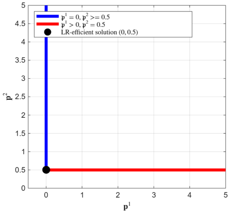
Let $A_1:=\{-2,-1,0,1\}$ and $A_2:=\left\{{\displaystyle \frac{1}{6}},{\displaystyle \frac{1}{2}},1,2,3\right\}$. Now, we consider a finite set $B\subseteq {\mathbb{H}}^2$, defined as follows:

$$B:=\left\{\mathfrak{p}=({\mathfrak{p}}^1,{\mathfrak{p}}^2)\in {\mathbb{H}}^2:{\mathfrak{p}}^1\in A_1,{\mathfrak{p}}^2\in A_2\right\}.$$

We then employ Algorithm 1 to find LR-efficient solutions of (P₃) using MATLAB R2024b. The numerical results of Algorithm 1 are presented in Table 1.

Table 1. LR-efficient Solution of ($P_3$) using Algorithm 1.

S. No.	Data Points	Feasibility	KKT Conditions	Emptiness $({\mathcal{M}}_{+0}^{+}\left(\mathfrak{q}\right)\cup {\mathcal{M}}_{00}^{+}\left(\mathfrak{q}\right)\cup {\widehat{\mathcal{M}}}_{0+}^{-}\left(\mathfrak{q}\right)=\mathit{\varnothing })$	Optimality	CPU Time (seconds)
1.	(-1, 0.167)	No	-	-	-	0.61
2.	(-1,0.5)	No	-	-	-
3.	(-1, 1)	No	-	-	-
4.	(-1, 2)	No	-	-	-
5.	(-1, 3)	No	-	-	-
6.	(0, 0.167)	No	-	-	-
7.	(0, 0.5)	Yes	Satisfied	Yes	LR-efficient solution
8.	(0, 1)	Yes	Not Satisfied	-	-
9.	(0, 2)	Yes	Not Satisfied	-	-
10.	(0, 3)	Yes	Not Satisfied	-	-
11.	(1, 0.167)	No	-	-	-
12.	(1, 0.5)	Yes	Not Satisfied	-	-
13.	(1, 1)	No	-	-	-
14.	(1,2)	No	-	-	-
15.	(1,3)	No	-	-	-
16.	(-2, 0.167)	No	-	-	-
17.	(-2,0.5)	No	-	-	-
18.	(-2,1)	No	-	-	-
19.	(-2,2)	No	-	-	-
20.	(-2,3)	No	-	-	-

Table 1. LR-efficient Solution of ($P_3$) using Algorithm 1.

S. No.	Data Points	Feasibility	KKT Conditions	Emptiness $({\mathcal{M}}_{+0}^{+}\left(\mathfrak{q}\right)\cup {\mathcal{M}}_{00}^{+}\left(\mathfrak{q}\right)\cup {\widehat{\mathcal{M}}}_{0+}^{-}\left(\mathfrak{q}\right)=\mathit{\varnothing })$	Optimality	CPU Time (seconds)
1.	(-1, 0.167)	No	-	-	-	0.61
2.	(-1,0.5)	No	-	-	-
3.	(-1, 1)	No	-	-	-
4.	(-1, 2)	No	-	-	-
5.	(-1, 3)	No	-	-	-
6.	(0, 0.167)	No	-	-	-
7.	(0, 0.5)	Yes	Satisfied	Yes	LR-efficient solution
8.	(0, 1)	Yes	Not Satisfied	-	-
9.	(0, 2)	Yes	Not Satisfied	-	-
10.	(0, 3)	Yes	Not Satisfied	-	-
11.	(1, 0.167)	No	-	-	-
12.	(1, 0.5)	Yes	Not Satisfied	-	-
13.	(1, 1)	No	-	-	-
14.	(1,2)	No	-	-	-
15.	(1,3)	No	-	-	-
16.	(-2, 0.167)	No	-	-	-
17.	(-2,0.5)	No	-	-	-
18.	(-2,1)	No	-	-	-
19.	(-2,2)	No	-	-	-
20.	(-2,3)	No	-	-	-

5. Conclusions and Future Research Directions

This article investigated a class of nonsmooth interval-valued multiobjective programming problems with vanishing constraints (NIMPPVC) in the Hadamard manifold setting, where the objective and constraint functions are assumed to satisfy locally Lipschitz continuity hypotheses. It has been derived that the various standard constraint qualifications, in particular, Cottle-type, Slater-type, Mangasarian-Fromovitz-type, and linearly independent constraint qualifications, are violated at any arbitrary feasible point of NIMPPVC. We have introduced several NIMPPVC-tailored constraint qualifications, namely ACQ-VC, GACQ-VC, GGCQ-VC, CCQ-VC, SCQ-VC, MFCQ-VC, and LICQ-VC, and further established interrelations among them. By employing GGCQ-VC, we have established the KKT-type necessary optimality conditions for LR-efficient solutions of NIMPPVC via Clarke subdifferentials. Moreover, sufficient criteria of optimality for LR-efficient solutions of NIMPPVC have been derived under generalized geodesic convexity assumptions. An algorithm has been proposed to identify the LR-efficient solutions of NIMPPVC. Various illustrative examples on Hadamard manifolds are furnished to highlight the significance of the results derived in this paper.

The findings presented in this paper generalize several known results available in the existing literature. For instance, the results established in this paper generalize the results derived by Achtziger and Kanzow [1] from the setting of Euclidean space to the Hadamard manifold framework and from MPVC to NIMPPVCs. Various results concerning constraint qualifications and optimality criteria for NIMPPVCs generalize the corresponding results established by Maeda [45] from the framework of Euclidean space to the Hadamard manifold setting, as well as from smooth multiobjective optimization problems to NIMPPVCs. Moreover, several results related to constraint qualifications established in this paper generalize the corresponding results derived by Mishra et al. [6] from the Euclidean space setting to the Hadamard manifold framework, as well as from smooth multiobjective MPVCs to NIMPPVCs. Furthermore, the results presented in this paper extend the corresponding findings of Upadhyay and Ghosh [37] from smooth multiobjective MPVCs to NIMPPVCs within the Hadamard manifold framework. In addition to this, results related to constraint qualifications for NIMPPVC in this paper generalize the corresponding results established by Ghosh et al. [36] from smooth multiobjective optimization problems to NIMPPVCs.

The results established in this paper suggest various options for research avenues. In view of the fact that for a locally Lipschitz continuous function, the limiting subdifferential provides a better Lagrange multiplier rule as compared to the Clarke subdifferential and is the smallest among all robust subdifferentials (see, [54]), various results related to optimality conditions for NIMPPVC established in this paper could be further sharpened by employing limiting subdifferentials in the framework of Riemannian manifolds.

References

- Achtziger, W.; Kanzow, C. Mathematical programs with vanishing constraints: Optimality conditions and constraint qualifications. Math. Program. 2008, 114(1), 69–99. [Google Scholar] [CrossRef]
- Hoheisel, T.; Kanzow, C. Stationary conditions for mathematical programs with vanishing constraints using weak constraint qualifications. J. Math. Anal. Appl. 2008, 337, 292–310. [Google Scholar] [CrossRef]
- Hoheisel, T.; Kanzow, C. On the Abadie and Guignard constraint qualifications for mathematical programs with vanishing constraints. Optimization 2009, 58, 431–448. [Google Scholar] [CrossRef]
- Hoheisel, T.; Kanzow, C. First- and second-order optimality conditions for mathematical programs with vanishing constraints. Appl. Math. 2007, 52, 495–514. [Google Scholar] [CrossRef]
- Latombe, J.C. Robot Motion Planning; Kluwer: Norwell, MA, USA, 1991. [Google Scholar]
- Mishra, S.K.; Singh, V.; Laha, V.; Mohapatra, R.N. On constraint qualifications for multiobjective optimization problems with vanishing constraints. In Optimization Methods, Theory and Applications; Xu, H., Wang, S., Wu, S.Y., Eds.; Springer: Berlin, Germany, 2015; pp. 95–135. [Google Scholar]
- Sadeghieh, A.; Kanzi, N.; Caristi, G.; Barilla, D. On stationarity for nonsmooth multiobjective problems with vanishing constraints. J. Glob. Optim. 2022, 82(4), 929–949. [Google Scholar] [CrossRef]
- Antczak, T. Optimality results for nondifferentiable vector optimization problems with vanishing constraints. J. Appl. Anal. Comput. 2023, 13(5), 2613–2629. [Google Scholar] [CrossRef] [PubMed]
- Moore, R.E. Methods and Applications of Interval Analysis; SIAM: Philadelphia, PA, USA, 1979. [Google Scholar]
- Moore, R.E. Computational Functional Analysis; Ellis Horwood Limited: England, 1985. [Google Scholar]
- Gutjahr, W.J.; Pichler, A. Stochastic multi-objective optimization: A survey on non-scalarizing methods. Ann. Oper. Res. 2016, 236(2), 475–499. [Google Scholar] [CrossRef]
- Shih, H.S.; Lai, Y.J.; Lee, E.S. Fuzzy approach for multi-level programming problems. Comput. Oper. Res. 1996, 23, 73–91. [Google Scholar] [CrossRef]
- Wu, H.C. The Karush–Kuhn–Tucker optimality conditions in multiobjective programming problems with interval-valued objective functions. Eur. J. Oper. Res. 2009, 196, 49–60. [Google Scholar] [CrossRef]
- Upadhyay, B.B.; Stancu-Minasian, I.M.; Sain, S.; Mishra, P. Generalized Minty and Stampacchia vector variational-like inequalities and interval-valued vector optimization problems. In Continuous Optimization and Variational Inequalities; Jayswal, A., Antczak, T., Eds.; Chapman and Hall/ CRC: New York, 2022; pp. 199–221. [Google Scholar]
- Jayswal, A.; Stancu-Minasian, I.-M.; Banerjee, J. Optimality conditions and duality for interval-valued optimization problems using convexifactors. Rend. Circ. Mat. Palermo. 2016, 65(1), 17–32. [Google Scholar] [CrossRef]
- Upadhyay, B.B.; Stancu-Minasian, I.M.; Mishra, P. On relations between nonsmooth interval-valued multiobjective programming problems and generalized Stampacchia vector variational inequalities. Optimization 2023, 72(10), 2635–2659. [Google Scholar] [CrossRef]
- Upadhyay, B.B.; Pandey, R.K.; Liao, S. Newton’s method for interval-valued multiobjective optimization problem. J. Ind. Manag. Optim. 2024, 20, 1633–1661. [Google Scholar] [CrossRef]
- Upadhyay, B.B.; Sain, S.; Stancu-Minasian, I.M. Lagrange duality and saddle point optimality conditions for nonsmooth interval-valued multiobjective semi-infinite programming problems with vanishing constraints. Axioms 2024, 13, 1–45. [Google Scholar] [CrossRef]
- Jayswal, A.; Stancu-Minasian, I.-M.; Banerjee, J. On interval-valued programming problem with invex functions. J. Nonlinear Convex Anal. 2016, 17(3), 549–567. [Google Scholar]
- Antczak, T.; Upadhyay, B.B.; Mohapatra, R.N. Optimality conditions and duality results for nondifferentiable vector interval-valued optimization problems with G-invex functions. Rend. Circ. Mat. Palermo II. Ser. 2026, 75(108), 1–25. [Google Scholar] [CrossRef]
- Jayswal, A.; Stancu-Minasian, I.M.; Banerjee, J.; Stancu, A.M. Sufficiency and duality for optimization problems involving interval-valued invex function in parametric form. Oper. Res. Int. J. 2015, 15, 137–161. [Google Scholar] [CrossRef]
- Singh, D.; Dar, B.A.; Kim, D.S. KKT optimality conditions in interval-valued multiobjective programming with generalized differentiable functions. Eur. J. Oper. Res. 2016, 254, 29–39. [Google Scholar] [CrossRef]
- Antczak, T. Optimality conditions and duality results for nonsmooth vector optimization problems with multiple interval-valued objective function. Acta Math. Sci. Ser. B Engl. Ed. 2017, 37, 1133–1150. [Google Scholar] [CrossRef]
- Absil, P.-A.; Mahony, R.; Sepulchre, R. Optimization Algorithms on Matrix Manifolds; Princeton University Press: Princeton, NJ, USA, 2009. [Google Scholar]
- Belkin, M.; Niyogi, P. Semi-supervised learning on Riemannian manifolds. Mach. Learn. 2004, 56, 209–239. [Google Scholar] [CrossRef]
- Arsigny, V.; Fillard, P.; Pennec, X.; Ayache, N. Geometric means in a novel vector space structure on symmetric positive-definite matrices. SIAM J. Matrix Anal. Appl. 2007, 29(1), 328–347. [Google Scholar] [CrossRef]
- Sommer, S.; Lauze, F.; Hauberg, S.; Nielsen, M. Manifold valued statistics, exact principal geodesic analysis and the effect of linear approximations. In Computer Vision–ECCV 2010, Lecture Notes in Computer Science; Daniilidis, K., Maragos, P., Paragios, N., Eds.; Springer: Berlin, Germany, 2010; pp. 43–56. [Google Scholar]
- Pennec, X. Manifold valued image processing with SPD matrices. In Riemannian Geometric Statistics in Medical Image Analysis; Pennec, X., Sommer, S., Fletcher, T., Eds.; Elsevier: Amsterdam, The Netherlands, 2020; pp. 75–134. [Google Scholar]
- Udrişte, C. Convex Functions and Optimization Methods on Riemannian Manifolds; Springer: Berlin, Germany, 2013. [Google Scholar]
- Papa Quiroz, E.A.; Quispe, E.M.; Oliveira, P.R. Steepest descent method with a generalized Armijo search for quasiconvex functions on Riemannian manifolds. J. Math. Anal. Appl. 2009, 341, 467–477. [Google Scholar] [CrossRef]
- Ferreira, O.P.; Louzeiro, M.S.; Prudente, L.F. Gradient method for optimization on Riemannian manifolds with lower bounded curvature. SIAM J. Optim. 2019, 29, 2517–2541. [Google Scholar] [CrossRef]
- Sakai, T. Riemannian Geometry; American Mathematical Society: Providence, RI, USA, 1996. [Google Scholar]
- Tung, L.T.; Singh, V. Optimality conditions and duality for mathematical programming with equilibrium constraints including multiple interval-valued objective functions on Hadamard manifolds. Jpn. J. Indust. Appl. Math. 2024, 41, 1105–1136. [Google Scholar] [CrossRef]
- Upadhyay, B.B.; Li, L.; Mishra, P. Nonsmooth interval-valued multiobjective optimization problems and generalized variational inequalities on Hadamard manifolds. Appl. Set.-Valued Anal. Optim. 2023, 5, 69–84. [Google Scholar] [CrossRef]
- Chen, S. The KKT optimality conditions for optimization problem with interval-valued objective functions on Hadamard manifolds. Optimization 2022, 71, 613–632. [Google Scholar] [CrossRef]
- Ghosh, A.; Upadhyay, B.B.; Stancu-Minasian, I.M. Constraint qualifications for multiobjective programming problems on Hadamard manifolds. Aust. J. Math. Anal. Appl. 2023, 20, 1–18. [Google Scholar] [CrossRef]
- Upadhyay, B.B.; Ghosh, A. On constraint qualifications for mathematical programming problems with vanishing constraints on Hadamard manifolds. J. Optim. Theory Appl. 2023, 199, 1–35. [Google Scholar] [CrossRef]
- Nguyen, L.T.; Chang, Y.L.; Hu, C.C.; Chen, J.S. Optimality and KKT conditions for interval-valued optimization problems on Hadamard manifolds. Optimization 2024, 74, 1–33. [Google Scholar] [CrossRef]
- Hosseini, S.; Pouryayevali, M.R. Generalized gradients and characterization of epi-Lipschitz sets in Riemannian manifolds. Nonlinear Anal. 2011, 74, 3884–3895. [Google Scholar] [CrossRef]
- Karkhaneei, M.M.; Mahdavi-Amiri, N. Nonconvex weak sharp minima on Riemannian manifolds. J. Optim. Theory Appl. 2019, 183, 85–104. [Google Scholar] [CrossRef]
- Chryssochoos, I.; Vinter, R.B. Optimal control problems on manifolds: A dynamic programming approach. J. Math. Anal. Appl. 2003, 287, 118–140. [Google Scholar] [CrossRef]
- Ledyaev, Y.S.; Zhu, Q.J. Nonsmooth analysis on smooth manifolds. Trans. Amer. Math. Soc. 2007, 359, 3687–3732. [Google Scholar] [CrossRef]
- Hosseini, S. Optimality conditions for global minima of nonconvex functions on Riemannian manifolds. Pac. J. Optim. 2015, 1–12. [Google Scholar]
- Upadhyay, B.B.; Ghosh, A.; Treanţa, S. Constraint qualifications and optimality criteria for nonsmooth multiobjective programming problems on Hadamard manifolds. J. Optim. Theory Appl. 2024, 200, 794–819. [Google Scholar] [CrossRef]
- Maeda, T. Constraint qualifications in multiobjective optimization problems: Differentiable case. J. Optim. Theory Appl. 1994, 80(3), 483–500. [Google Scholar] [CrossRef]
- Moore, R.E. Interval Analysis; Prentice-Hall: Englewood Cliffs, NJ, USA, 1966. [Google Scholar]
- Barani, A. Generalized monotonicity and convexity for locally Lipschitz function on Hadamard manifolds. Differ. Geom.-Dyn. Syst. 2013, 15, 26–37. [Google Scholar]
- Upadhyay, B.B.; Poddar, S. Optimality conditions and duality for robust nonsmooth multiobjective semi-infinite optimization problem on Hadamard manifolds. Appl. Anal. Optim. 2024, 8, 167–201. [Google Scholar]
- Chen, S.-I.; Fang, C.-J. Vector variational inequality with pseudoconvexity on Hadamard manifolds. Optimization 2016, 65, 2067–2080. [Google Scholar] [CrossRef]
- Tung, L.T.; Tam, D.H. Optimality conditions and duality for multiobjective semi-infinite programming on Hadamard manifolds. Bull. Iran. Math. Soc. 2022, 48, 2191–2219. [Google Scholar] [CrossRef]
- Li, X.F. Constraint qualifications in nonsmooth multiobjective optimization. J. Optim. Theory Appl. 2000, 106, 373–398. [Google Scholar] [CrossRef]
- Clarke, F.H. Optimization and Nonsmooth Analysis; Wiley-Interscience: New York, NY, USA, 1983. [Google Scholar]
- Upadhyay, B.B.; Ghosh, A.; Treanţa, S. Optimality conditions and duality for nonsmooth multiobjective semi-infinite programming problems with vanishing constraints on Hadamard manifolds. J. Math. Anal. Appl. 2023, 531, 1–25. [Google Scholar] [CrossRef]
- Mordukhovich, B.S. Variational Analysis and Generalized Differentiation I. Basic Theory; Springer-Verlag: Berlin, Germany, 2006. [Google Scholar]
Figure 1.
Interrelations among the constraint qualifications for NIMPPVC.
Disclaimer/Publisher’s Note: The statements, opinions and data contained in all publications are solely those of the individual author(s) and contributor(s) and not of MDPI and/or the editor(s). MDPI and/or the editor(s) disclaim responsibility for any injury to people or property resulting from any ideas, methods, instructions or products referred to in the content. |
© 2026 by the authors. Licensee MDPI, Basel, Switzerland. This article is an open access article distributed under the terms and conditions of the Creative Commons Attribution (CC BY) license (http://creativecommons.org/licenses/by/4.0/).
Copyright: This open access article is published under a Creative Commons CC BY 4.0 license, which permit the free download, distribution, and reuse, provided that the author and preprint are cited in any reuse.