

Submitted:
26 August 2026
Posted:
28 August 2026
You are already at the latest version
Abstract
Monitoring and forecasting environmental thresholds in data-scarce ecosystems poses a critical challenge for resource management. In this study, we evaluate four forecasting paradigms—Seasonal Autoregressive Integrated Moving Average (SARIMA), Light Gradient Boosting Machine (LightGBM), Long Short-Term Memory (LSTM) networks, and Echo State Networks (ESNs)—to model and reconstruct historical landing dynamics of a shallow-water shrimp fishery. The historical time series exhibits severe data gaps, including continuous unmonitored periods spanning up to six years. To assess real-time deployment feasibility, all models were benchmarked on an embedded NVIDIA Jetson Orin Nano edge platform using walk-forward validation (h=1). Empirical results demonstrate that the ESN architecture captures the non-linear temporal dynamics of the fishery, achieving the highest predictive accuracy (MAE=1.37t, RMSE=1.96t, and RMSSE=0.70). A bidirectional forecasting-backcasting reconstruction strategy filled the multi-year gaps and confirmed that the landing decline occurred abruptly after 2013. For edge computing applications, the ESN achieved low latency, executing sub-millisecond inference (0.27ms) and a fast training time per fold (424.44ms) while consuming less energy than LSTM. These findings indicate that projecting dynamics into a high-dimensional fixed reservoir provides a computationally efficient solution for continuous time-series reconstruction and landing trend detection under severe data and hardware constraints.
Keywords:
echo state networks
; edge AI
; fisheries forecasting
; JAX
; reservoir computing
; shallow-water shrimp
1. Introduction
Modern socio-ecological system (SES) models encounter significant challenges due to high-dimensional interactions and non-linear dynamics that can hinder sustainable decision-making [1]. These complex dynamics generate feedbacks and critical regime thresholds [2], where variability in noisy time series can obscure biological reorganizations [3,4], making long-term monitoring and global sensitivity analysis essential to mitigate analytical bias [1,5]. A representative case is the tropical shrimp fishery, where the transition from artisanal methods to large-scale industrial trawling altered benthic habitats and food webs [6,7,8]. Overexploitation and environmental degradation have subsequently driven severe landing declines in tropical regions [9,10], often characterized by landing drops below of historical maximums and accompanying socio-ecological instability [11].
Recent studies have documented severe landing declines across tropical and subtropical shrimp fisheries driven by cumulative fishing pressure and management challenges, as observed in Brazil [12], Tanzania [13], and Bangladesh [14]. In the Colombian Caribbean, industrial shrimp trawling initiated during the 1960s and expanded during the 1970s and 1980s, supported by favorable market margins and international demand [15]. During its historical peak, this fleet constituted one of the primary industrial marine sectors in the region, where the deployment of Florida-type trawlers equipped with double-rigged nets increased sweep efficiency and operational catchability [15,16].
Limited data availability has historically hindered precise stock assessments and the implementation of effective management measures, preventing the application of robust evaluation models [17]. Consequently, the cumulative impacts of overexploitation were not detected in time, becoming evident in the late 1990s when reported landings began a sustained decline. Operational constraints, including exchange rate fluctuations, escalating fuel costs, and aquaculture market competition, led to the official closure of the fishery in 2005. The daily operational dynamics of commercial fleets yield highly noisy datasets with an elevated percentage of missing values [18,19], structured as complex, high-dimensional time series [20,21,22,23] that present a critical challenge for conventional predictive frameworks [24,25].
Traditional listwise deletion or linear interpolation methods are inadequate and introduce bias when applied to non-linear dynamic time series, as they ignore underlying missing data distributions and distort system trajectories by omitting temporal correlations [26]. In non-linear systems, the loss of temporal continuity compromises structural representation by failing to capture higher-order dependencies [19,21]. To address these limitations, the Reservoir Computing (RC) framework integrates an input layer, a non-linear dynamic reservoir with fixed randomized weights, and a linear readout layer [18,20]. Its primary computational advantage lies in training exclusively the output weights through linear optimization, such as Ridge regression or regularized least squares [21,25,27,28]. By avoiding backpropagation through time (BPTT) [29], the RC paradigm ensures rapid convergence without vanishing gradient phenomena and with low computational overhead, making it suitable for deployment on edge devices [26,30]. Furthermore, its capacity to manage data loss relies on iterative schemes grounded in fixed-point convergence, enabling the recovery of structural dynamics without exhaustive preprocessing [18,19,20,24].
Echo State Networks (ESN) represent a prominent Reservoir Computing framework for processing temporal data [23,30] by employing fixed, randomized weight matrices () and training exclusively the output readout layer via linear optimization [18,20]. Dynamical stability relies on satisfying the Echo State Property (ESP) with spectral radius [20,26,30], enabling phase-space reconstruction and imputation in highly variable time series without BPTT, even under elevated missing data rates () or near non-linear transition thresholds [18,19,24,26,30,31]. To overcome Python execution constraints [32,33], functional differentiable programming via JAX [34] integrates automatic differentiation (grad) [35], explicit array vectorization (vmap) [36], and Just-In-Time (JIT) compilation powered by OpenXLA [37,38]. This implementation optimizes memory throughput and computational overhead through kernel operator fusion [39], achieving execution efficiency comparable to low-level C++/CUDA implementations [40,41]. Deploying a JAX-native ESN on an NVIDIA Jetson Orin Nano edge device enables real-time inference and dynamic variable imputation [33,39,41,42], supporting the historical landing series reconstruction of the Colombian Caribbean industrial shrimp fishery under a missing data rate of [43].
Despite these methodological advances, two gaps remain in the application of Reservoir Computing to data-scarce fisheries monitoring. First, comparative benchmarks of ESNs against conventional forecasting baselines (SARIMA, LightGBM, LSTM) have rarely been conducted under a strict edge-deployment constraint that jointly considers predictive accuracy, inference latency, memory footprint, and energy consumption. Second, while imputation-capable reservoir architectures have been proposed for missing data recovery [18,26], their use for long-range, bidirectional historical reconstruction of collapsed or discontinued fisheries—where monitoring gaps exceed one-third of the observed record—remains largely unexplored, particularly in tropical small-scale fisheries with fragmented statistical systems [43].
To address these gaps, this study proposes an edge-optimized ESN framework implemented in JAX and evaluates it through two distinct experimental tasks applied to the historical landing series of the Colombian Caribbean industrial shrimp fishery. The first task addresses the question of which model offers the best one-step-ahead forecasting performance under a strict out-of-sample Walk-Forward Validation (WFV) scheme, benchmarking the JAX-native ESN against SARIMA, LightGBM, and LSTM baselines in terms of predictive accuracy (MAE, RMSE, RMSSE) and edge-deployment cost (latency, memory, energy) on an NVIDIA Jetson Orin Nano. The second task addresses the distinct question of whether a bidirectional ESN architecture can retrospectively reconstruct large, structurally discontinuous historical gaps (missing data rate of ) in the same series, providing a continuous landing trajectory suitable for exploratory comparison against independent biological and stock-assessment evidence, without being used as a substitute for formal stock assessment.
The main contributions of this work are threefold: (i) a systematic, hardware-aware benchmark of Reservoir Computing against conventional statistical and deep learning baselines for fisheries time-series forecasting under small-data regimes; (ii) a bidirectional ESN reconstruction protocol for long-gap univariate marine landing series, evaluated independently from the forecasting task; and (iii) an open, energy- and latency-characterized deployment of a JAX-native ESN on embedded edge hardware, establishing a reproducible computational baseline for autonomous, low-resource fisheries monitoring systems.
2. Materials and Methods
2.1. Historical Landing Records (1993–2023)
Landings of Shallow-Water Shrimp (SWS) taken by the industrial trawl fleet along the Colombian Caribbean coast comprise several commercial taxa, including Penaeus notialis, Penaeus schmitti, Penaeus brasiliensis, Penaeus subtilis, Trachypenaeus similis, Trachypenaeus constrictus, Xiphopenaeus kroyeri, and Penaeus monodon [43,44]. A historical database containing monthly landing records from 1993 to 2023 was analyzed [43]. Data processing involved descriptive analyses at annual and monthly scales, including inter- and intra-annual comparisons of total landings and taxonomic composition.
The historical trajectory of reported landings shows a peak during the late 1990s, reaching a maximum of in 1997, followed by a decline that led to an operational collapse between 2000 and 2005 (Figure 1). Figure 1 also shows extensive observational gaps resulting from administrative and operational disruptions. The empirical landing distribution exhibits a strong positive skewness (Figure 2), demonstrating that the fishery operated predominantly at low yield levels (between 0 and ), whereas high landing values () corresponded to isolated events prior to the decline in catches.
Intra-annual variability evaluated across months (January to December) reflects a seasonal pattern during historical high-landing periods, characterized by catch peaks in February, April, and December (Figure 3). Over the last decade, this seasonal signal flattened near zero, indicating a suppression of intra-annual landing fluctuations.
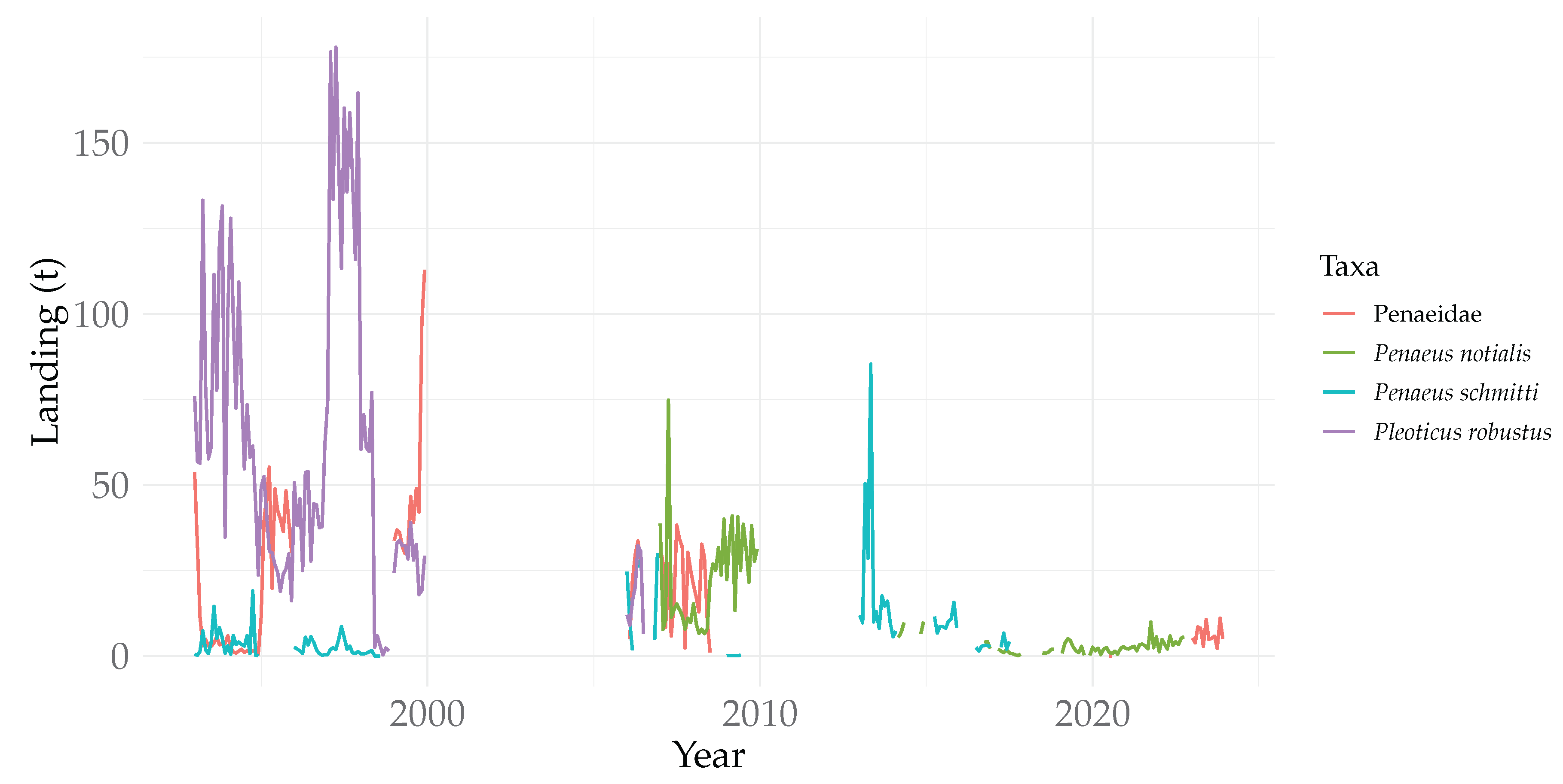
The taxonomic breakdown highlights shifts in taxon contributions and temporal dominance (Figure A1), notably the prominence of Pleoticus robustus during the late 1990s. Disaggregating these trajectories into individual panels (Figure 4) reveals taxon-specific landing dynamics and reporting discontinuities, demonstrating that the decline did not affect all reported categories uniformly or simultaneously.
Comparative boxplot distributions (Figure 5) confirm that Pleoticus robustus exhibited the highest median landings and interquartile ranges across the time series, whereas taxa such as Penaeus schmitti and Penaeus notialis maintained consistently lower and narrower distributions.
Table 1 summarizes the descriptive statistics for global landings and individual target taxa. All analyzed variables exhibit strong positive skewness, with mean values exceeding their respective medians. At the taxonomic level, Pleoticus robustus recorded the highest median landings () and a historical maximum of . Conversely, Penaeus species (P. notialis and P. schmitti) yielded lower values, with medians of and , respectively. The dataset shows missing observations across taxa, ranging from in P. notialis to in the general Penaeidae category.
2.1.1. Reconstructed Time Series Baseline
To enable rigorous benchmarking against classical statistical and machine learning models that strictly require complete time series without missing values, a fully reconstructed historical landing dataset was generated for the 1993–2023 period. Prior to imputation, a domain-specific temporal feature matrix was engineered to allow the non-parametric missForest algorithm [45] to capture complex temporal dynamics without imposing parametric assumptions. The target landing variable was contextualized by incorporating a continuous time index () to model secular long-term trends; an interannual component (year); a categorical factor variable representing calendar months (); and harmonic sinusoidal transformations ( and , where m denotes the calendar month) to eliminate artificial boundary discontinuities between December and January.
Data imputation in R (version 4.2.2) [46] using the missForest package (version 1.6.1) was executed with 300 trees (), 3 variables randomly sampled at each split (), and a maximum limit of 15 iterations (). Driven by this explicit temporal and seasonal representation, the imputation scheme yielded low internal imputation error, achieving a Normalized Root Mean Squared Error (NRMSE) of for continuous variables and a Proportion of Falsely Classified (PFC) entries of for categorical variables.
As shown in Figure 6, the imputed series restores temporal continuity across historical administrative gaps while preserving non-linear trajectories, peak events, and operational collapse dynamics. The statistical summary of the reconstructed dataset is presented in Table 2, yielding a complete set of monthly observations ( missing values) with a mean of and a median of , providing a fully gap-filled baseline for traditional benchmark models.
2.2. Experimental Scenarios and Dataset Partitioning
To evaluate model performance under realistic operational conditions and standardized benchmark configurations, an experimental scenario was designed using the reconstructed historical landing time series (). To ensure a temporally consistent forecasting evaluation, the monthly historical landing time series ( observations spanning January 1993 to December 2023) was chronologically partitioned into training, validation, and test subsets (Table 3). The training split encompasses 25 years (1993–2017, months, ), serving as the historical learning window. The validation set covers 3 years (2018–2020, months, ) for hyperparameter tuning and early stopping. Finally, an independent out-of-sample test set spanning 3 years (2021–2023, months, ) was reserved strictly for final performance evaluation.
To quantify the influence of the reconstruction stage, the proportion of reconstructed observations was calculated for each data partition. Most reconstructed values were concentrated within the historical training period (127 of 300 observations; 42.33%), corresponding to long monitoring interruptions prior to 2018. In contrast, the independent test partition contained only 2 reconstructed observations (5.56%), indicating that 94.44% of the final out-of-sample evaluation was based on directly observed landing records. Therefore, the reported forecasting performance is predominantly supported by empirical observations rather than imputed values. The scenario utilizes the fully reconstructed historical landing dataset generated via non-parametric imputation with missForest (Figure 6), enabling a fair and consistent comparison among forecasting architectures under identical data conditions.
As shown in Table 4, this scenario reflects a regime shift in recent years. While historical training records (1993–2017) exhibit higher catch levels (mean of ), the validation (2018–2020) and test (2021–2023) periods show lower landing values ( and , respectively). The non-parametric imputation procedure preserves the distributional properties, quantiles, and extreme bounds of each partition without inducing variance collapse or tail distortion.
To evaluate the stationarity properties and order of integration of the target landing time series prior to model training, Augmented Dickey-Fuller (ADF) unit root tests were performed using the tseries package (version 0.10-62) [47] on the raw series (excluding missing values) and on the reconstructed series across both the full 1993–2023 observation window () and the isolated training partition (). Across the entire evaluation period, the raw observed series rejected the unit root null hypothesis (, , , ). Similarly, the reconstructed series exhibited mean-reverting behavior (, , , ). These test statistics indicate that the imputation procedure preserved the overall mean-reverting properties without introducing deterministic linear trend artifacts into the univariate series.
2.2.1. Walk-Forward Validation
To prevent data leakage and simulate a realistic operational deployment, model parameters and hyperparameters were evaluated using Walk-Forward Validation (WFV) with a rolling-origin evaluation scheme [48]. Unlike standard k-fold cross-validation—which violates temporal dependencies by randomizing observations—the WFV protocol preserves chronological directionality [49]. Under this framework, parameter estimation at any target time step t relies exclusively on observable historical data.
The sequence evaluation procedure is formalized by establishing an initial training window of length , defining the operational observations required for model initialization and stable feature scaling. At each iteration i, the model utilizes the historical landings subsequence to generate multi-step out-of-sample forecasts over an h-step horizon, defined as . Following forecast generation over h, the forecast origin advances by s discrete time steps (). An expanding window strategy is implemented, wherein subsequent training iterations cumulatively integrate historical observations from preceding steps, enabling the model to adapt to structural variations and non-stationary trends in reported landings as new data become available.
The paired sequence of predicted and observed landings y generated at each forecast origin is stored sequentially to construct the out-of-sample error matrix. Predictive accuracy is quantified by aggregating forecasting discrepancies across all evaluated temporal folds, providing an empirical assessment of model generalization capacity under operational deployment conditions.
2.3. Bidirectional Landing Reconstruction Experiment
To evaluate the capability of the ESN to capture the underlying non-linear dynamics and temporal dependencies of reported landings from fragmented observations, a bidirectional reconstruction experiment was designed using the raw landing time series. The historical record was partitioned into three continuous subseries corresponding to effective monitoring periods: (1993–2000), (2006–2009), and (2013–2023). Table 5 presents the statistical summary for each subseries. The reconstruction of data gaps between adjacent subseries was performed using a dual-estimation strategy combining an autonomous forward forecast (forecasting) from the antecedent subseries () and a reversed backward forecast (backcasting) from the subsequent subseries (). This approach leverages the high-dimensional dynamics of the reservoir in both temporal directions, mitigating error accumulation inherent to long-term recursive forecasting over intervals with high missing data density. This procedure was applied exclusively to the ESN architecture to evaluate its intrinsic capacity for time-series reconstruction in data-scarce settings.
To ensure smooth continuity across the boundaries of observed data and eliminate structural discontinuities at the center of the unmonitored gaps, the bidirectional forecasts were integrated using a soft temporal weighting scheme. For each time step within a missing interval of length T, the consolidated estimate is defined as:
where the linear decay weight decreases monotonically from 1 to 0 according to:
Through this formulation, the prediction assigns higher confidence to the forward forecast near block and transitions smoothly toward reliance on the backward forecast near the boundary of , preserving physical continuity and local temporal dynamics at the edges of the observed data.
2.4. NVIDIA Jetson Orin Nano
To evaluate edge deployment feasibility and operational efficiency, inference and temporal validation were executed on an NVIDIA Jetson Orin Nano embedded module (8 GB variant). This platform features a 6-core Arm Cortex-A78AE v8.2 CPU running at a nominal frequency of 1.5 GHz (up to 1.73 GHz) and an NVIDIA Ampere architecture GPU with 1024 CUDA cores and 32 Tensor cores. Hardware acceleration for vectorized matrix operations and non-linear state updates is provided within this system, which is required for the real-time execution of recurrent reservoir computing architectures.
The platform integrates 8 GB of unified LPDDR5 memory shared across the CPU and GPU cores, alongside an NVMe solid-state drive (SSD) to deliver the throughput required for continuous data ingestion without volatile memory bottlenecks. Memory consumption metrics reported during execution reflect resource allocations within this shared physical RAM pool. Operating within a configurable power budget of 7–15 W (15 W mode enabled), the system provides an energy-efficient deployment platform suitable for integration into autonomous environmental monitoring stations and field-level edge acquisition systems.
The software execution environment was standardized on NVIDIA JetPack 6.2.3 (L4T R36.5.2) running Linux Kernel 6.8 (aarch64), accelerated via CUDA Toolkit 12.6. Model inference and reservoir dynamics were natively compiled and executed in Python using JAX (v0.5.2) configured with full CUDA GPU backend support (CudaDevice). The technical characterization of the hardware and software stack is detailed in Table 6.
2.5. Model Architecture and Edge Optimization
The ESN architecture comprises three distinct processing stages: a fixed input mapping, a dynamic non-linear reservoir, and a linear output readout layer. Mathematically, the continuous state space and output transformations are defined by an input weight matrix , a recurrent internal adjacency matrix , and an output readout weight matrix .
The discrete-time dynamics of the reservoir internal state are updated according to the non-linear state transition equation:
where:
- represents the vector of reported landing features at time step ;
- is the leaking rate governing system memory dissipation across temporal scales;
- denotes the input scaling factor controlling the degree of non-linearity activated within the reservoir state space;
- is the bias vector, and serves as the element-wise non-linear activation function mapping inputs into a high-dimensional state space (Equation (4)).
To ensure system stability and maintain the fading memory property, the reservoir state space must satisfy the ESP. This guarantees that the internal state representation evolves as a unique function of the historical input sequence while asymptotically dissipating initial state influences. Mathematically, a sufficient condition for ESP compliance is enforced by scaling the internal recurrent adjacency matrix W such that its spectral radius satisfies .
The training phase is restricted to optimizing the readout weight matrix . This step maps the concatenated reservoir state matrix to the target reported landing matrix using Ridge regression ( Tikhonov regularization) to prevent overfitting and ensure numerical stability during matrix inversion:
where denotes the Tikhonov regularization parameter and I represents the identity matrix.
2.5.1. Hyperparameter Tuning and Experimental Setup
Input sequences were constructed using a lag depth of historical observations to project the univariate landing signal into a high-dimensional recurrent reservoir space (). Hyperparameter selection and reservoir initialization were implemented following the guidelines of Lukoševičius (2012) [50].
To configure internal network dynamics and prevent temporal data leakage, a grid search was conducted using a forward-chaining cross-validation split. The search space included settings for reservoir capacity , leaking rate , spectral radius , input scaling , and Ridge regularization coefficient . The optimal combination was selected based on the lowest Mean Squared Error (MSE) of validation predictions, evaluated on non-imputed historical landing data.
To remove transient initialization artifacts, a washout period of steps was discarded before fitting the readout model. The readout parameters were estimated via closed-form Ridge regression (Tikhonov regularization) using direct matrix inversion, which provides low computational overhead suitable for edge devices. The complete structural hyperparameters, dynamic settings, and operational parameters configured for the JAX-accelerated ESN architecture are detailed in Table 7.
2.6. Baseline Models
To evaluate the predictive performance of the proposed ESN relative to established modeling approaches, three baseline architectures were implemented: a linear seasonal autoregressive baseline, a tree-based ensemble framework, and a deep recurrent neural network.
2.6.1. Seasonal Autoregressive Integrated Moving Average
To model the statistical properties of the time series, a Seasonal Autoregressive Integrated Moving Average (SARIMA) model was evaluated as a linear benchmark. Hyperparameter selection and order estimation for seasonal and non-seasonal autoregressive, differencing, and moving average components were performed using the pmdarima library (version 2.1.1) [51] through Akaike Information Criterion (AIC) minimization. Table 8 outlines the parameter estimates and diagnostic metrics for the fitted model evaluated on the landing time series (). Although most parameters achieved statistical significance () and residual autocorrelation was reduced (Ljung-Box , ), the Jarque-Bera test statistic (, ) indicates heavy-tailed residual behavior, reflecting the abrupt regime shifts present in historical landing data.
2.6.2. Light Gradient Boosting Machine
To evaluate non-linear tree-based ensemble methods, LightGBM was implemented using the lightgbm library (version 4.7.0) [52]. Because Gradient Boosted Decision Trees (GBDT) lack intrinsic sequential memory, temporal dependencies were explicitly incorporated by extracting autoregressive lags alongside calendar features. The predictor matrix includes historical target lags ( through ) in conjunction with temporal covariates—specifically year, month, and sine/cosine cyclical encoding—to capture multi-scale seasonality and long-term landing trends.
Structural hyperparameters were tuned using randomized search with temporal forward-chaining cross-validation (TimeSeriesSplit) evaluating parameter combinations on the training set, optimizing for Root Mean Squared Error (RMSE). To mitigate overfitting, an early stopping criterion of 100 boosting rounds monitored against the validation set was enforced during hyperparameter tuning and final model training. The optimal hyperparameter configuration is summarized in Table 9. Regularization penalties ( and ), feature fractioning, and subsampling were applied to constrain tree depth and prevent overfitting under data-scarce conditions.
2.6.3. Long Short-Term Memory
A Long Short-Term Memory (LSTM) recurrent neural network was evaluated as a deep learning benchmark for sequential modeling. To reformulate the time series into a supervised learning structure, a sliding-window approach was applied, constructing input sequences of consecutive historical timesteps () to predict the single-step-ahead landing value (). The architecture was implemented using Keras (version 3.15.1) [53] with JAX as the computational backend. The JAX framework enabled accelerated network training and Backpropagation Through Time (BPTT) via JIT compilation and vectorized operations, ensuring computational efficiency during evaluation.
The network topology comprises an initial LSTM layer with ReLU activation, followed by a Dropout regularization layer and a dense linear output layer. Hyperparameter selection was conducted via random search across sampled configurations from a discrete search space spanning hidden unit capacities , learning rates , batch sizes , training epochs , and dropout rates . Models were compiled using Mean Squared Error (MSE) loss and trained with the Adam optimizer. The optimal candidate was selected based on the minimal RMSE computed on denormalized validation predictions. Table 10 details the resulting optimal configuration, comprising trainable parameters.
2.7. Performance Metrics
To evaluate predictive accuracy across scale-dependent and scale-independent dimensions, both point-error metrics and relative scaled forecasting indicators were implemented. Initial forecasting accuracy was quantified using the Mean Absolute Error (MAE) and the Root Mean Squared Error (RMSE), defined in Equations (6) and (7), respectively:
While RMSE imposes a quadratic penalty that heavily weights larger forecast errors, MAE provides a linear assessment that is less sensitive to extreme transient peaks. However, because the historical landing series exhibits pronounced positive skewness, intermittency, and near-zero values (Figure 2)—a statistical distribution analogous to the intermittent demand series analyzed in the M5 forecasting competition [54]—standard scale-dependent metrics alone are insufficient to evaluate model performance across varying catch dynamics without bias.
To address these constraints, performance was also evaluated using the Root Mean Squared Scaled Error (RMSSE) [55], defined as:
The RMSSE scales the out-of-sample mean squared error of the forecast against the in-sample mean squared error of a first-order Naïve random-walk model [56]. This metric provides two main methodological advantages for fisheries time series: it is scale-independent, allowing comparison across different scenarios, and it avoids division-by-zero singularities that destabilize percentage-based metrics during zero-catch or low-landing periods.
3. Results
3.1. Static Benchmark Performance
Table 11 presents the comparative evaluation of predictive performance across candidate architectures throughout the training, validation, and testing phases. Regarding global predictive accuracy, the ESN architecture demonstrates superior performance, achieving the lowest test error metrics with a MAE of , RMSE of , and RMSSE of . This indicates the capacity of the dynamic reservoir to capture complex non-linear patterns without overfitting. LightGBM exhibits competitive test performance (MAE of , RMSE of ), while recording the lowest training error (MAE of , RMSE of ). Conversely, SARIMA (test MAE of ) and LSTM (test MAE of ) display substantially higher errors, highlighting the limitations of linear statistical formulations and the convergence challenges of deep recurrent architectures on this dataset scale.
When evaluating computational efficiency during real-time execution, LightGBM demonstrates the lowest processing latency, recording a mean sample latency of ms/sample across validation and test sets. This processing rate is approximately four times faster than ESN and SARIMA () and over five times faster than LSTM (). All tested architectures maintain sub-millisecond execution latencies during the testing phase, supporting their preliminary technical feasibility for deployment on resource-constrained embedded monitoring systems.
Regarding memory consumption, LightGBM maintained the lowest baseline system RAM occupancy () across all evaluated execution splits. The ESN architecture preserved a stable baseline system memory load of , exhibiting only a minor dynamic memory peak during training () associated with state matrix allocation, which was completely released during inference (). In contrast, SARIMA exhibited the highest baseline system RAM load ( in testing), whereas LSTM required the largest peak allocation during training (). These empirical findings support the use of ESN when maximum predictive precision is required, while LightGBM represents an effective alternative for deployment scenarios with stringent latency and computational constraints.
3.2. Trajectory Analysis and Physical Domain Consistency
Figure 7 illustrates the temporal trajectory of predicted landing series across all evaluated models, while Table 12 summarizes their descriptive statistical properties over their respective effective evaluation sample sizes. A fundamental operational requirement for physical consistency in fishery landing forecasting is the non-negativity of catch predictions (). Linear baseline models failed to strictly satisfy this domain constraint; SARIMA yielded unphysical negative values down to , and LightGBM also crossed the zero threshold with a minimum of . Conversely, both recurrent architectures—LSTM () and ESN ()—preserved strictly positive predictions, demonstrating inherent stability in low-density regimes.
Regarding distributional behavior, all candidate architectures matched the right-skewed nature of the target landing series (), maintaining central values consistent with historical landings (). However, discrepancies arose in the reconstruction of extreme peak events (Max). While LightGBM exhibited severe oversmoothing by truncating peak values at , ESN () and LSTM () tracked high-amplitude nonlinear spikes without numerical explosion or dynamic range attenuation. Finally, the effective evaluation sample sizes for ESN () and LSTM () reflect the initial truncation induced by sequence lookback requirements () and the initial transient state discard period ().
Statistical significance tests revealed a trade-off between in-sample fitting and out-of-sample generalization. During the training period (1993–2017), LightGBM exhibited lower fitting errors than the ESN model, as confirmed by positive Diebold-Mariano statistics ( for squared error; for absolute error). Across the out-of-sample validation and test period (2018–2023), however, the performance trend reversed, and the JAX-based ESN achieved superior predictive accuracy compared to LightGBM. The Diebold-Mariano test yielded negative statistics for both squared-error loss () and absolute-error loss (), rejecting the null hypothesis of equal forecast accuracy. The paired Wilcoxon signed-rank test further confirmed that the ESN model produced a significantly smaller median absolute error (). These results show that while LightGBM overfits when trained on tabular lag structures, the ESN architecture maintains dynamic generalization under time-varying conditions, supporting its suitability for operational deployment.
3.3. Walk-Forward Validation
To ensure a strictly equal baseline comparison, all models (SARIMA, LightGBM, LSTM, and ESN) were evaluated exclusively on the fully reconstructed dataset () generated via missForest.
Table 13 presents the evaluation metrics under the Walk-Forward Validation (WFV) scheme, which models sequential real-time deployment conditions through one-step-ahead () retraining and inference. The ESN yielded the lowest overall error metrics, attaining a MAE of , RMSE of , and RMSSE of . This performance demonstrates the ability of the dynamic reservoir to update its readout weights via Ridge regression at each iterative step. SARIMA (MAE of ) and LSTM (MAE of ) showed lower errors than in static evaluation baselines, whereas LightGBM recorded a MAE of and RMSE of .
For computational efficiency and potential edge-device retraining, LightGBM recorded the lowest overall execution time () and average latency per evaluation fold (). The ESN displayed comparable temporal efficiency, processing evaluation folds in (), which represents a minor computational trade-off given its forecast accuracy gains under the WFV protocol. Conversely, the LSTM required () due to backpropagation through time and computation graph operations. SARIMA proved operationally unfeasible for continuous edge deployment, requiring () due to iterative ARIMA parameter re-estimation at each step.
Regarding memory dynamics during WFV, LightGBM and LSTM maintained zero net memory leakage (), with LightGBM maintaining overall system usage at . The ESN exhibited minor state dynamic variation () due to reservoir state matrix updating, keeping overall system memory occupancy stable at . Although SARIMA exhibited the lowest initial baseline memory footprint () due to the absence of deep learning framework dependencies, it showed significant state accumulation over continuous iterations (), indicating potential memory growth over extended deployment horizons.
Power profiling revealed distinct thermal and electrical behaviors across architectures. While average power consumption remained within a narrow band across all algorithms ( to ), the LSTM recorded the highest transient power peak (), driven by burst GPU compute cycles during recurrent backpropagation. Evaluating total energy expenditure () highlighted the operational efficiency of reservoir computing: LightGBM and ESN consumed and , respectively, across the WFV scheme. In contrast, the LSTM consumed (), and SARIMA required (). Consequently, the ESN provided an effective balance between predictive precision and energy efficiency for resource-constrained edge hardware.
3.4. Bidirectional Landing Reconstruction Results
The ESN-based bidirectional reconstruction strategy successfully imputed the unmonitored historical gaps (2000–2005 and 2010–2012) (Figure 1, Table 1). As illustrated in Figure 8, the reconstructed landing trajectory preserves the temporal variability and dynamics observed in adjacent subseries.
As summarized in Table 14, the reconstructed time series ( monthly observations) exhibits a mean of (), ranging from to . For the 107 reconstructed observations, confidence intervals derived from the ensemble dispersion of multiple reservoir initializations indicate bounded uncertainty, with a mean lower boundary of for the confidence interval and a mean upper boundary of .
3.4.1. Seasonal Patterns and Dynamic Transition
During the first reconstructed interval (2000–2005), the ESN architecture captured both the long-term memory and the seasonal fluctuations characteristic of the fishery landing records. Following the cessation of monitoring in February 2000, when a relative peak of was recorded, the reconstructed trajectory exhibited a progressive attenuation while preserving intra-annual oscillations. Systematic increases in reported landing levels occurred during the final quarter of each year and the initial months of the following year, reaching secondary peaks of in July 2002 alongside recurring recoveries in early 2003 and 2004 at and , respectively. These upward trends were followed by moderate mid-year troughs, culminating in a decline to in November 2005 prior to the junction with subseries .
This behavior indicates that the high-dimensional state space of the reservoir performs geometric interpolation between boundaries while projecting the dominant frequencies learned during training on subseries . Soft Temporal Weighting () eliminated sharp discontinuities at the center of the imputation blocks, ensuring a smooth transition into in 2006.
3.4.2. Uncertainty Behavior and Resource Status
The morphology of the confidence intervals (Figure 8) displays an hourglass pattern consistent with dynamic systems theory: uncertainty remains minimal near the boundaries adjacent to observed subseries ( and ) and reaches its maximum amplitude at the center of the gap (around 2002–2003 and 2011), where the temporal distance to real observations is greatest.
Regarding fishery dynamics, the continuous reconstruction confirms that throughout the 2000–2012 period, relative landing levels remained above the operational landing-based collapse threshold of ( of historical maximum landing). The lower boundary of the confidence interval () touched this critical threshold only during brief transition states in late 2005. This indicates that the subsequent decline in reported landings occurred rapidly after 2013 rather than as a continuous degradative process during the unmonitored years.
3.5. Model Stability and Seed Sensitivity Analysis
To evaluate whether the reconstruction performance is dependent upon favorable random state initializations, a comprehensive seed sensitivity analysis was conducted across ten independent random instances (). For each seed , the internal weight matrices (W and ) were stochastically generated utilizing JAX pseudo-random keys, while maintaining all structural hyperparameters strictly constant ().
As detailed in Table 15, the WFV metrics exhibited exceptional stability across all evaluated seeds and error formulations. The MAE yielded an average performance of with a minimal standard deviation of (ranging from a minimum of to a maximum of ). Similarly, the RMSE demonstrated high consistency, averaging (). Finally, the RMSSE confirmed these findings with an average value of and a negligible standard deviation of ().
This marginal variance across all considered error norms indicates that the high-dimensional state space generated by the reservoir, in conjunction with Ridge regression (), achieves a robust and consistent representation of the underlying dynamics irrespective of the initial stochastic configuration. Consequently, the ESN architecture demonstrates substantial structural robustness, ensuring that the predictive performance of the reconstructed time series remains invariant to initialization fluctuations.
Furthermore, computational tracking demonstrates the efficiency and scalability of the underlying implementation. The validation procedure for the initial execution (Seed 0) required seconds, with subsequent evaluations maintaining an almost identical computational cost and stabilizing at an average execution time of seconds per complete validation sequence. This highly consistent processing time, devoid of significant initial compilation overheads, confirms the computational suitability and reliability of the proposed framework for deployment in resource-constrained edge architectures.
4. Discussion
The results obtained from both the static partition and the sequential WFV demonstrate that the ESN achieves competitive predictive accuracy, structural robustness, and computational efficiency when modeling non-stationary landing time series characterized by high variability and a high frequency of zero-value observations.
In the static evaluation scheme, the ESN achieved the lowest testing error among all evaluated architectures, recording an , an , and an . These metrics reflect a substantial performance improvement over traditional linear statistical baselines (SARIMA: , ), standard tree-based ensemble methods (LightGBM: , ), and deep recurrent baselines (LSTM: , ). While linear and autoregressive baselines exhibited pronounced structural degradation during periods of rapid landing fluctuations, the recurrent dynamic structure of the ESN captured complex non-linear interactions without suffering from overfitting or phase-lag artifacts.
Under the sequential walk-forward validation scheme (), where models were continuously updated with new temporal observations, the performance advantage of the ESN framework became more pronounced. The ESN attained an , an , and an . An RMSSE below indicates that the ESN outperforms the baseline Naïve benchmark by approximately , effectively handling data sparsity and volatile landing yields. This performance stems from the online adaptation capability of the linear readout layer via Ridge regression, which allows the network to track local temporal regime shifts without retraining the fixed internal reservoir weights.
Deep learning baselines such as the LSTM (, under WFV) demonstrated competitive pattern recognition capabilities but required higher computational complexity and memory allocation (). Conversely, while LightGBM executed rapidly during training, it failed to generate realistic continuous trajectories over multi-step or out-of-sample prediction horizons, frequently predicting negative landing values (). In contrast, the internal state dynamics of the ESN constrained predicted values within physically plausible domain boundaries (), preserving the operational logic of the fishery landing series.
Regarding the pronounced discrepancy observed in tree-based ensemble baselines, such as the training-to-validation error divergence in LightGBM (training MAE of versus validation MAE of , as detailed in Table 11, this behavior highlights a fundamental limitation of static machine learning models under structural breaks. Because the evaluation protocol establishes a strict temporal partition to test out-of-distribution generalization, the transition from the training period to validation and test horizons encompasses a shift in the underlying dynamical regime. Although standard regularization constraints (specified in Table 9) prevented excessive tree growth during training, LightGBM relies on axis-aligned split decisions over static feature spaces, rendering it incapable of extrapolating temporal trajectories when the statistical properties of the data change post-training. Consequently, the apparent overfitting is not merely a failure of hyperparameter tuning, but a structural vulnerability of tabular learning algorithms when confronted with non-stationary time series transitions. In contrast, the recurrent reservoir dynamics of the ESN absorb these regime shifts by projecting temporal histories into a high-dimensional continuous manifold.
Statistical significance testing confirmed the quantitative advantage of the proposed ESN architecture. Both the Diebold–Mariano test and the non-parametric Wilcoxon signed-rank test indicated statistically significant differences () in predictive error distributions when comparing the ESN against SARIMA and LightGBM on out-of-sample data. While the error difference between the ESN and the LSTM was narrower in certain folds, the ESN achieved competitive accuracy at a fraction of the computational and time cost during training and inference.
Analysis of the ESN bidirectional temporal reconstruction reveals a clear distinction between operational decline and catch-based variations within the fishery timeline. Specifically, the operational decline observed around 2005—characterized by the cessation of monitoring and a sharp reduction in industrial fleet activity—represented an economic and operational contraction driven by exogenous macroeconomic pressures, including fuel price fluctuations and fleet dynamics. As evidenced by the bidirectional ESN reconstruction, where the mean reconstructed landing remained at , well above the landing-based operational threshold of , positive landing levels were nevertheless sustained throughout the unmonitored window of 2000–2012. In contrast, the post-2013 trajectory constitutes a sustained catch-based decline. Governed by cumulative exploitation patterns and compounding environmental variability, landings persistently decreased toward near-zero values—falling below in the test set—thereby indicating the firm persistence of a low-yield regime within the reported records.
Notably, the slight upward inflection observed at the terminal end of the reconstructed series is consistent with recent independent biological evidence for the same stock. Paramo et al. [57] reported low exploitation rates (–) for pink shrimp (Penaeus notialis) in the Colombian Caribbean, attributing this to the drastic reduction of the industrial trawling fleet to approximately five vessels, and suggested that the stock could be undergoing a recovery phase. This convergence between a purely data-driven reconstruction and an independent stock assessment strengthens confidence that the terminal signal reflects a genuine biological trend rather than a modeling artifact.
Beyond numerical error metrics, the contrast in predictive performance across historical periods can be interpreted through the principles of non-linear dynamical systems. Framing the initial monitoring phase () as a volatile dynamic regime suggests a system governed by sensitivity to initial conditions, characterized by a positive maximal Lyapunov exponent (). Under this theoretical framing, the Lyapunov prediction horizon () is restricted, rendering autonomous forward forecasting across extensive multi-year gaps challenging without bidirectional soft constraints. Conversely, following the catch-based decline post-2013 (), the system transitioned into a low-variance, stable state. This dynamical stabilization corresponds to a reduced divergence rate and an extended predictability horizon, explaining why predictive metrics stabilize during this era.
From an architectural standpoint, the Echo State Network mirrors these dynamical constraints. The reservoir weight matrix satisfies the ESP, which mathematically guarantees the Fading Memory Property by ensuring that the internal conditional Lyapunov exponents of the network remain negative. This intrinsic property forces the reservoir to exponentially decay the influence of distant past states, preventing distant noise from corrupting current state estimations while maintaining the short- to medium-term non-linear dynamics required for reliable bidirectional reconstruction.
Furthermore, the stability of the evaluation metrics across multiple random initializations (Table 15) provides empirical evidence of the structural robustness of the proposed ESN framework. In Reservoir Computing, stochastic weight generation (W and ) can introduce performance variability across different random seeds. However, the consistent response observed in these sensitivity trials demonstrates that the combination of a high-dimensional state space (), an appropriate spectral radius (), and Ridge regularization () projects the non-stationary landing dynamics into a stable manifold where the readout optimization converges reliably. This deterministic behavior indicates that the reconstructed subseries are governed by the intrinsic non-linear memory of the historical data, supporting the reliability of the model for data recovery.
Finally, despite the performance demonstrated under univariate fishery conditions, several inherent methodological limitations exist. First, the benchmark dataset was reconstructed using missForest prior to model comparison. Although this approach was necessary to provide a common complete dataset for SARIMA, LightGBM, and LSTM baselines, a potential source of bias may arise from the imputation stage itself. Nevertheless, only 5.6% of the observations in the independent test partition required reconstruction, indicating that the final out-of-sample evaluation was overwhelmingly supported by directly observed landing records.
Second, because the analytical framework relies exclusively on a univariate historical time series without exogenous covariates (such as environmental, climatic, or economic indicators), the capacity of the model to anticipate structural regime shifts driven entirely by external factors remains constrained. Second, regarding scalability and extreme non-stationarity, while a fixed reservoir size () proved adequate for capturing the temporal dependencies of this specific single-variable domain, scaling the architecture to handle high-dimensional multivariate inputs would require expanding the input weight matrix dimensions and re-tuning the spectral radius to prevent chaotic state saturation under severe distribution shifts. Future work will focus on integrating multi-source exogenous streams and optimizing adaptive reservoir scaling algorithms for multi-variable edge deployments.
5. Conclusions
Under small-data regimes, RC implemented via an ESN demonstrated competitive forecasting accuracy compared with an autoregressive baseline (SARIMA), a gradient-boosted decision tree ensemble (LightGBM), and a conventional recurrent neural network (LSTM). Evaluated under a strictly out-of-sample WFV protocol (), the ESN configuration yielded a MAE of , a RMSE of , and a RMSSE of , reducing forecasting error by relative to the non-seasonal naive baseline (). The consistency of predictive metrics across temporal validation partitions indicates that the non-linear dynamic reservoir captures complex temporal patterns without exhibiting catastrophic overfitting.
From the perspective of edge intelligence deployed on embedded hardware (NVIDIA Jetson Orin Nano), the experimental benchmark established a Pareto frontier among predictive accuracy, latency, and memory footprint. Although LightGBM proved to be the least resource-intensive model, with an inference latency of and a system RAM usage of , the ESN provided a competitive trade-off by recording sub-millisecond inference latency () and a training time of per fold. Compared with the high latency of the LSTM () caused by BPTT and graph recompilation, as well as the high operational cost of SARIMA ( with a RAM accumulation of ), the ESN updates its weights through an exact linear ridge regression.
Although average instantaneous power draw remains comparable across model families, the LSTM consumes approximately 43 times more total energy than the ESN to complete the WFV task. This energy footprint indicates that the ESN is a more energy-efficient solution for autonomous edge monitoring systems powered by batteries or photovoltaic panels.
The high-dimensional state space generated by the fixed reservoir allows the network to map complex non-linear temporal dynamics—such as industrial shrimp landings—even in the presence of continuous missing data gaps. Operating on univariate time series, the bidirectional ESN framework provides historical reconstruction and enables identification of the post-2013 landing decline threshold, with the terminal recovery signal consistent with independent stock-level evidence for the same fishery [57].
The ESN implementation in JAX using 64-bit precision demonstrates that over-parameterized deep learning models or linear autoregressive methods are unnecessary for edge time-series forecasting. Projecting input dynamics into a high-dimensional fixed reservoir while updating only the linear readout layer constitutes an efficient strategy for continuous monitoring under hardware and data constraints.
Author Contributions
Conceptualization, D.R.-L., M.E.I.-M., P.F.-C., M.C.C.-M., J.A. and H.Z.; methodology, D.R.-L., M.E.I.-M. and P.F.-C.; software, D.R.-L., M.E.I.-M. and P.F.-C.; validation, D.R.-L., M.E.I.-M., P.F.-C., M.C.C.-M., J.A. and H.Z.; formal analysis, D.R.-L., M.E.I.-M., P.F.-C., M.C.C.-M., J.A. and H.Z.; investigation, M.C.C.-M., J.A. and H.Z.; resources, M.C.C.-M.; data curation, M.C.C.-M. and D.R.-L.; writing—original draft preparation, D.R.-L. and J.A.; writing—review and editing, D.R.-L., M.E.I.-M., P.F.-C., M.C.C.-M., J.A. and H.Z.; visualization, D.R.-L., M.E.I.-M. and P.F.-C. All authors have read and agreed to the published version of the manuscript.
Funding
This research was funded by the Universidad Cooperativa de Colombia under project code INV3797 (“Hacia el pronóstico de los desembarcos de las pesquerías artesanales del Caribe colombiano”), awarded to D.R.-L.; the Generalitat Valenciana (Spain) through PROMETEO grant CIPROM/2023/32, awarded to P.F.-C.; and the Conselleria de Educación, Cultura, Universidades y Empleo of the Generalitat Valenciana (Reference CIAPOS/2024/238, APOSTD/2025 - MODALIDAD A), co-funded by the European Social Fund Plus (FSE+) under the 2021–2027 Operational Programme of the Comunitat Valenciana, supporting M.E.I.-M. The funders had no role in the design of the study; in the collection, analyses, or interpretation of data; in the writing of the manuscript; or in the decision to publish the results.
Institutional Review Board Statement
Not applicable.
Informed Consent Statement
Not applicable.
Data Availability Statement
The data supporting the findings of this study are publicly available in the SEANOE repository [43] at https://www.seanoe.org/data/00928/104004/.
Acknowledgments
The authors express their sincere gratitude to the Autoridad Nacional de Acuicultura y Pesca (AUNAP) for providing open access to the fishery dataset utilized in this study. Additional institutional backing was provided by the Vice-Rector’s Office for Research of the Universidad del Magdalena in collaboration with the Universidad Cooperativa de Colombia within the framework of the project “Comparison of construction and operational parameters of three models of trawl systems in the Colombian Caribbean using computer simulations and empirical mathematical methods”.
Conflicts of Interest
The authors declare no conflicts of interest.
Abbreviations
The following abbreviations are used in this manuscript:
| ADF | Augmented Dickey-Fuller |
| AUNAP | Autoridad Nacional de Acuicultura y Pesca |
| BPTT | Backpropagation Through Time |
| CPU | Central Processing Unit |
| CUDA | Compute Unified Device Architecture |
| DM | Diebold–Mariano |
| ESN | Echo State Network |
| ESP | Echo State Property |
| FMP | Fading Memory Property |
| GBM | Gradient Boosting Machine |
| GPU | Graphics Processing Unit |
| JIT | Just-In-Time |
| LightGBM | Light Gradient Boosting Machine |
| LSTM | Long Short-Term Memory |
| MAE | Mean Absolute Error |
| MLE | Maximal Lyapunov Exponent |
| NRMSE | Normalized Root Mean Squared Error |
| PACF | Partial Autocorrelation Function |
| PFC | Proportion of Falsely Classified |
| RC | Reservoir Computing |
| RMSE | Root Mean Squared Error |
| RMSSE | Root Mean Squared Scaled Error |
| SARIMA | Seasonal Autoregressive Integrated Moving Average |
| SES | Socio-Ecological System |
| SWS | Shallow-Water Shrimp |
| WFV | Walk-Forward Validation |
| XLA | Accelerated Linear Algebra |
Appendix A. Taxonomic Composition of Historical Landing
This appendix provides temporal visualizations of the taxonomic breakdown for the shallow-water shrimp (SWS) fishery dataset from 1993 to 2023. Figure A1 shows the historical trajectories of landings across four main commercial taxonomic groups (Pleoticus robustus, Penaeus notialis, Penaeus schmitti, and aggregated Penaeidae). These trends show periods of species dominance, reporting gaps, and long-term changes in landing levels.
Figure A1.
Historical superposition of landing trajectories across major commercial SWS taxa.
References
- Huang, Y.; Halouani, G.; Luján, C.; Lasram, F.B.R.; Girardin, R. Global sensitivity analysis of a complex marine ecosystem model: Advancing the understanding of ecosystem functioning. Ecological Modelling 2026, 521, 111725. [CrossRef]
- Stelzenmüller, V.; Letschert, J.; Blanz, B.; Blöcker, A.M.; Claudet, J.; Cormier, R.; Gee, K.; Held, H.; Kannen, A.; Kruse, M.; et al. Exploring the adaptive capacity of a fisheries social-ecological system to global change. Ocean & Coastal Management 2024, 258, 107391. [CrossRef]
- Cano, A.V.; Jensen, O.P.; Dakos, V. Identifying fish populations prone to abrupt shifts via dynamical footprint analysis. Proceedings of the National Academy of Sciences 2025, 122, e2505461122. [CrossRef]
- Sguotti, C.; Bischoff, A.; Conversi, A.; Mazzoldi, C.; Möllmann, C.; Barausse, A. Stable landings mask irreversible community reorganizations in an overexploited Mediterranean ecosystem. Journal of Animal Ecology 2022, 91, 2465–2479. [CrossRef]
- Burbank, J.; Rolland, N.; McDermid, J.L.; Turcotte, F.; Tunney, T.D.; Ricard, D.; Sylvain, F.E. Substantial loss of trawlable biomass and lack of recovery in a marine ecosystem. Communications Biology 2025, 8, 831. [CrossRef]
- Guillet, R. Estudio mundial sobre las pesquerías del camarón. Available online: https://www.fao.org/4/i0300s/i0300s00.htm (accessed on 2026-07-15).
- Herrera-Valdivia, E.; López-Martínez, J.; Vargasmachuca, S.C. Estrés en la comunidad íctica en la pesca de arrastre del camarón en el norte del Golfo de California. Revista de Biología Tropical 2015, 63, 741–754.
- Zeller, D.; Cashion, T.; Palomares, M.; Pauly, D. Global marine fisheries discards: A synthesis of reconstructed data. Fish and Fisheries 2018, 19, 30–39. [CrossRef]
- Costello, C.; Gaines, S.D.; Lynham, J. Can Catch Shares Prevent Fisheries Collapse? Science 2008, 321, 1678–1681. [CrossRef]
- Pinsky, M.L.; Jensen, O.P.; Ricard, D.; Palumbi, S.R. Unexpected patterns of fisheries collapse in the world’s oceans. Proceedings of the National Academy of Sciences 2011, 108, 8317–8322. [CrossRef]
- De Mutsert, K.; Cowan, J.H.; Essington, T.E.; Hilborn, R. Reanalyses of Gulf of Mexico fisheries data: Landings can be misleading in assessments of fisheries and fisheries ecosystems. Proceedings of the National Academy of Sciences 2008, 105, 2740–2744. [CrossRef]
- Teodoro, S.; Da Silva Cortinhas, M.; Proietti, M.; Costa, R.; Dumont, L. High genetic connectivity among pink shrimp Farfantepenaeus paulensis (Pérez-Farfante, 1967) groups along the south-southeastern coast of Brazil. Estuarine, Coastal and Shelf Science 2020, 232, 106488. [CrossRef]
- Silas, M.O.; Mgeleka, S.S.; Kangwe, S.J. River discharge, fishing effort and catch composition of prawn fisheries in coastal Tanzania. Western Indian Ocean Journal of Marine Science 2023, 22, 135–145. [CrossRef]
- Alam, M.S.; Liu, Q.; Schneider, P.; Mozumder, M.M.H.; Uddin, M.M.; Monwar, M.M.; Hoque, M.E.; Barua, S. Stock Assessment and Rebuilding of Two Major Shrimp Fisheries (Penaeus monodon and Metapenaeus monoceros) from the Industrial Fishing Zone of Bangladesh. Journal of Marine Science and Engineering 2022, 10, 201. [CrossRef]
- Zúñiga, H.; Altamar, J.; Manjarrés, L. Caracterización tecnológica de la flota de arrastre camaronero del mar Caribe de Colombia. Proyecto Innovación Tecnológica de la Flota Industrial Camaronera del Mar Caribe de Colombia. Santa Marta 2004.
- Bustos, D.; Rueda, M.; Viaña, J.; Rodriguez, A.; Girón, A.; García, L.; Pardo, E. Evaluación interanual del impacto de las pesquerías industriales de arrastre de camarón sobre la biodiversidad marina de Colombia. In Proceedings of the annual Gulf and Caribbean Fisheries Institute, 2013, Vol. 65, pp. 370–374.
- De Barros, M.; Oliveira-Filho, R.; Aschenbrenner, A.; Hostim-Silva, M.; Chiquieri, J.; Schwamborn, R. Evaluation of traditional and bootstrapped methods for assessing data-poor fisheries: a case study on tropical seabob shrimp ( Xiphopenaeus kroyeri ) with an improved length-based mortality estimation method. PeerJ 2024, 12, e18397. [CrossRef]
- Tan, H.; Shi, L.; Wang, S.; Qu, S.X. Improving model-free prediction of chaotic dynamics by purifying the incomplete input. AIP Advances 2024, 14, 125225. [CrossRef]
- Liu, J.; Xu, X.; Li, E. Sample-weighted reservoir computing for chaotic dynamics prediction with a high proportion of missing data. Nonlinear Dynamics 2026, 114, 526. [CrossRef]
- Kuan, Y.H.; Narayanan, V.; Li, J.S. Iterative Reservoir Computing Networks for Reconstructing Irregular Time Series. IEEE Transactions on Neural Networks and Learning Systems 2025, 36, 14189–14200. [CrossRef]
- Shi, L.; Yan, Y.; Wang, H.; Wang, S.; Qu, S.X. Predicting chaotic dynamics from incomplete input via reservoir computing with ( D + 1 ) -dimension input and output. Physical Review E 2023, 107, 054209. [CrossRef]
- Baur, S.; Räth, C. Predicting high-dimensional heterogeneous time series employing generalized local states. Physical Review Research 2021, 3, 023215. [CrossRef]
- Yoshida, S.; Iinuma, T.; Nobukawa, S.; Watanabe, E.; Isokawa, T. Heterogeneous Assembly Echo State Networks for High-Dimensional, Multiscale Time Series: Dynamic Analysis via Delay Capacity and Multiscale Fuzzy Entropy. IEEE Access 2025, 13, 209299–209311. [CrossRef]
- Arbateni, K.; Benzaoui, A. Enhancing Heartbeat Classification through Cascading Next Generation and Conventional Reservoir Computing. Applied Sciences 2024, 14, 3030. [CrossRef]
- Özalp, E.; Nóvoa, A.; Magri, L. Real-time forecasting of chaotic dynamics from sparse data and autoencoders. Computer Methods in Applied Mechanics and Engineering 2026, 450, 118600. [CrossRef]
- Huang, F.; Zheng, W.; Guo, W.; Yu, Z. Estimating missing data for sparsely sensed time series with exogenous variables using bidirectional-feedback echo state networks. CCF Transactions on Pervasive Computing and Interaction 2023, 5, 45–63. [CrossRef]
- Hoerl, A.E.; Kennard, R.W. Ridge Regression: Biased Estimation for Nonorthogonal Problems. Technometrics 2000, 42, 80–86. [CrossRef]
- Girosi, F.; Jones, M.; Poggio, T. Regularization Theory and Neural Networks Architectures. Neural Computation 1995, 7, 219–269. [CrossRef]
- Vlachas, P.; Pathak, J.; Hunt, B.; Sapsis, T.; Girvan, M.; Ott, E.; Koumoutsakos, P. Backpropagation algorithms and Reservoir Computing in Recurrent Neural Networks for the forecasting of complex spatiotemporal dynamics. Neural Networks 2020, 126, 191–217. [CrossRef]
- Guo, W.; Li, S.; Liu, J.; Li, E.; Xu, X. Model-free analysis of complex systems using delayed-feedback echo state network. Physical Review E 2026, 114, 014204. [CrossRef]
- Li, X.; Zhu, Q.; Zhao, C.; Qian, X.; Zhang, X.; Duan, X.; Lin, W. Tipping Point Detection Using Reservoir Computing. Research 2023, 6, 0174. [CrossRef]
- The Python Language Reference. Available online: https://docs.python.org/3/reference/index.html (accessed on 2026-07-27).
- Enrico, R.; Mancini, M.; Capello, E. Comparison of NMPC and GPU-Parallelized MPPI for Real-Time UAV Control on Embedded Hardware. Applied Sciences 2025, 15, 9114. [CrossRef]
- Frostig, R.; Johnson, M.J.; Leary, C. Compiling machine learning programs via high-level tracing. In Proceedings of the Conference on Systems and Machine Learning (SysML), 2018.
- Wu, G. A framework for structural shape optimization based on automatic differentiation, the adjoint method and accelerated linear algebra. Structural and Multidisciplinary Optimization 2023, 66, 151. [CrossRef]
- Sapunov, G. Deep learning with JAX; Manning: Shelter Island, 2024.
- OpenXLA Project. Available online: https://openxla.org/?hl=es-419 (accessed on 2026-07-27).
- Wen, H.; Luo, F.; Xu, S.; Wang, B. JANC: A cost-effective, differentiable compressible reacting flow solver featured with JAX-based adaptive mesh refinement. Computer Physics Communications 2026, 319, 109915. [CrossRef]
- Tchakoute, R.N.; Tadonki, C.; Dokladal, P.; Mesri, Y. Benchmark-Based Study of CPU/GPU Power-Related Features Through JAX and TensorFlow. IEEE Access 2025, 13, 184543–184560. [CrossRef]
- NVIDIA Corporation. CUDA C++ Programming Guide. Technical report, NVIDIA, 2020.
- Ratul, I.J.; Zhou, Y.; Yang, K. Accelerating Deep Learning Inference: A Comparative Analysis of Modern Acceleration Frameworks. Electronics 2025, 14, 2977. [CrossRef]
- Saad, F.; Burnim, J.; Carroll, C.; Patton, B.; Köster, U.; A. Saurous, R.; Hoffman, M. Scalable spatiotemporal prediction with Bayesian neural fields. Nature Communications 2024, 15, 7942. [CrossRef]
- Cruz-Mercado, M.; Altamar, J.; Zúñiga, H. Historical Records of Shallow-Water Shrimp Landings in the Colombian Caribbean: 1993-2023. Available online: https://www.seanoe.org/data/00928/104004/ (accessed on 2026-07-16). [CrossRef]
- Gómez-Lemos, L.A.; Hernando Campos, N. PRESENCIA DE PENAEUS MONODON FABRICIUS (CRUSTACEA: DECAPODA: PENAEIDAE) EN AGUAS DE LA GUAJIRA COLOMBIANA. Boletín de Investigaciones Marinas y Costeras - INVEMAR 2008, 37, 221–225.
- Stekhoven, D.J.; Bühlmann, P. MissForest—non-parametric missing value imputation for mixed-type data. Bioinformatics 2012, 28, 112–118. [CrossRef]
- R Core Team. R: A Language and Environment for Statistical Computing. Available online: https://www.R-project.org/.
- Trapletti, A.; Hornik, K. tseries: Time Series Analysis and Computational Finance. Available online: https://CRAN.R-project.org/package=tseries. R package version 0.10-62.
- Tashman, L.J. Out-of-sample tests of forecasting accuracy: an analysis and review. International Journal of Forecasting 2000, 16, 437–450. [CrossRef]
- Cerqueira, V.; Torgo, L.; Mozetič, I. Evaluating time series forecasting models: an empirical study on performance estimation methods. Machine Learning 2020, 109, 1997–2028. [CrossRef]
- Lukoševičius, M. A practical guide to applying echo state networks. In Neural Networks: Tricks of the Trade: Second Edition; Springer, 2012; pp. 659–686. [CrossRef]
- Smith, T.G.; et al. pmdarima: ARIMA estimators for Python, 2017.
- Ke, G.; Meng, Q.; Finley, T.; Wang, T.; Chen, W.; Ma, W.; Ye, Q.; Liu, T.Y. LightGBM: A Highly Efficient Gradient Boosting Decision Tree. In Proceedings of the Advances in Neural Information Processing Systems; Guyon, I.; Luxburg, U.V.; Bengio, S.; Wallach, H.; Fergus, R.; Vishwanathan, S.; Garnett, R., Eds. Curran Associates, Inc., 2017, Vol. 30.
- Chollet, F.; et al. Keras. https://keras.io, 2015.
- Makridakis, S.; Petropoulos, F.; Spiliotis, E. Introduction to the M5 forecasting competition Special Issue. International Journal of Forecasting 2022, 38, 1279–1282. [CrossRef]
- Makridakis, S.; Spiliotis, E.; Assimakopoulos, V. M5 accuracy competition: Results, findings, and conclusions. International Journal of Forecasting 2022, 38, 1346–1364. [CrossRef]
- Makridakis, S.; Spiliotis, E.; Assimakopoulos, V. The M5 competition: Background, organization, and implementation. International Journal of Forecasting 2022, 38, 1325–1336. [CrossRef]
- Paramo, J.; Pérez, D.; Mildenberger, T. Growth and Mortality of the Pink Shrimp Penaeus notialis (Pérez Farfante, 1967)(Decapoda: Dendrobranchiata: Penaeidae) in the Colombian Caribbean. Marine Ecology 2025, 46, e12863. [CrossRef]
Figure 1.
Historical trajectory of Shallow-Water Shrimp (SWS) reported landings in the Colombian Caribbean industrial trawl fishery (1993–2023).
Figure 1.
Historical trajectory of Shallow-Water Shrimp (SWS) reported landings in the Colombian Caribbean industrial trawl fishery (1993–2023).
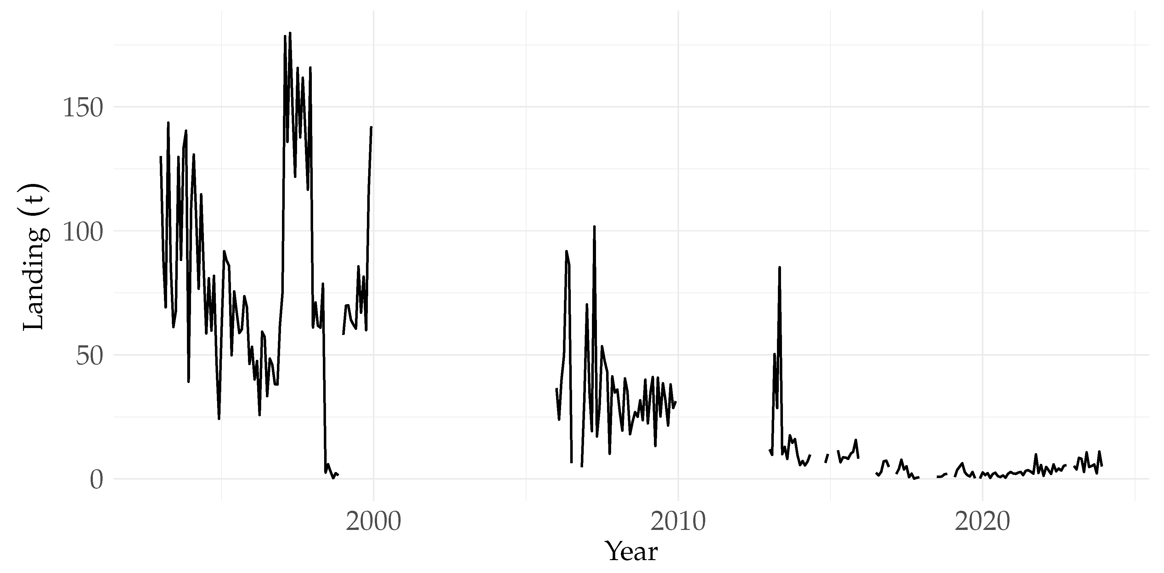
Figure 2.
Density distribution and positive skewness of historical landing values (t).
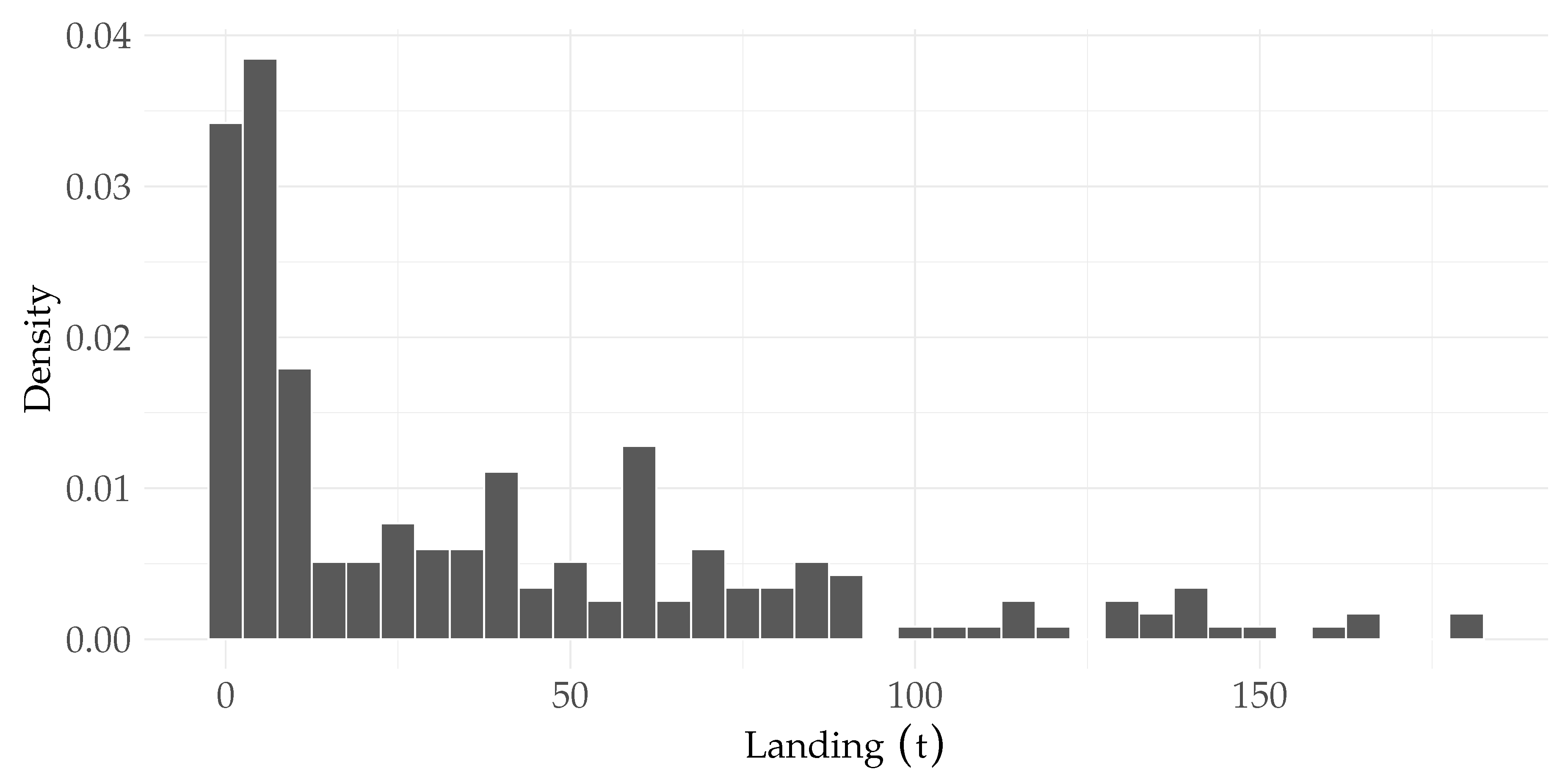
Figure 3.
Monthly seasonal variability of landing across different historical years.
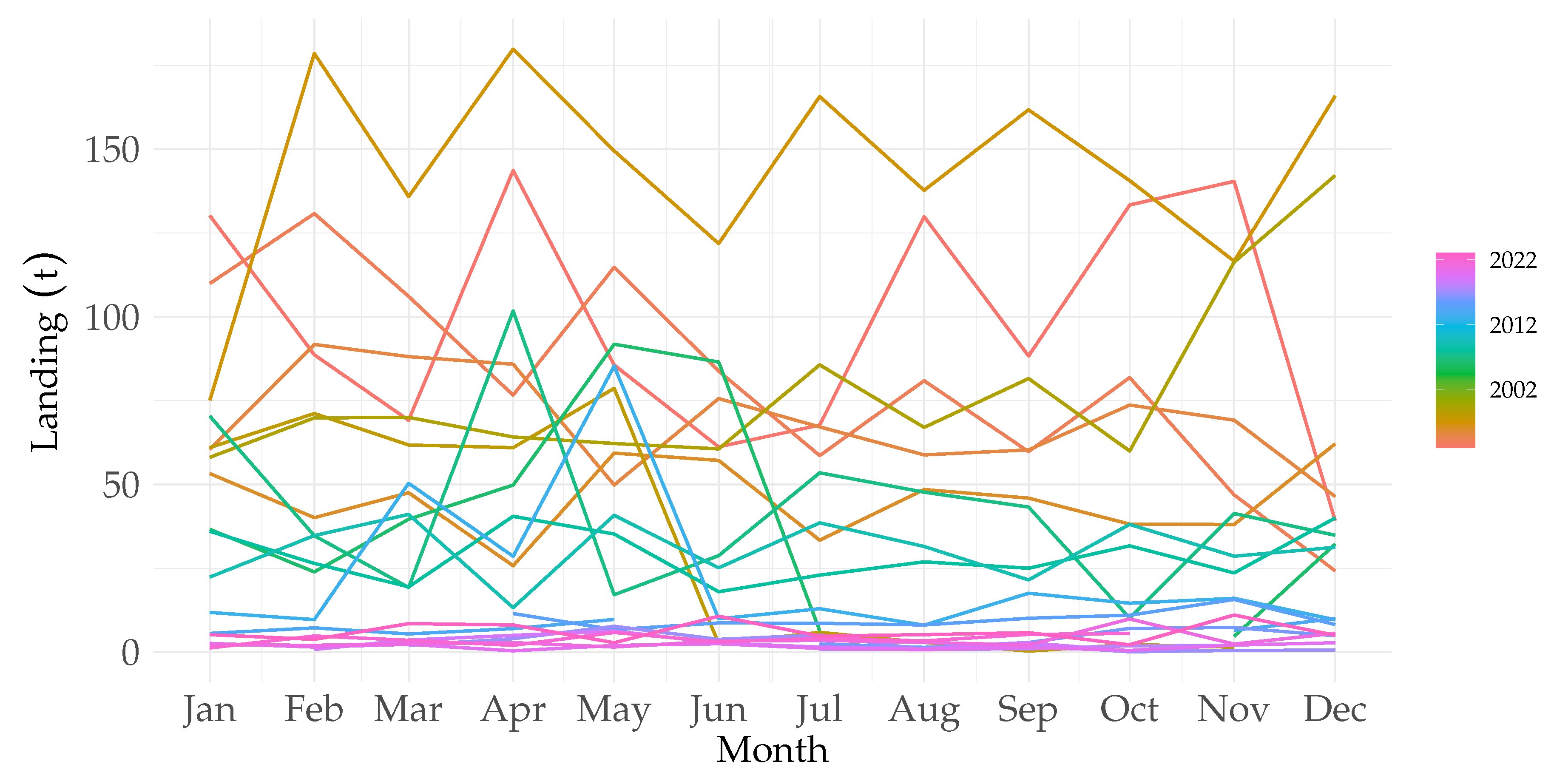
Figure 4.
Faceted temporal trajectories of individual SWS taxa illustrating species-specific dynamics and missing data periods.
Figure 4.
Faceted temporal trajectories of individual SWS taxa illustrating species-specific dynamics and missing data periods.
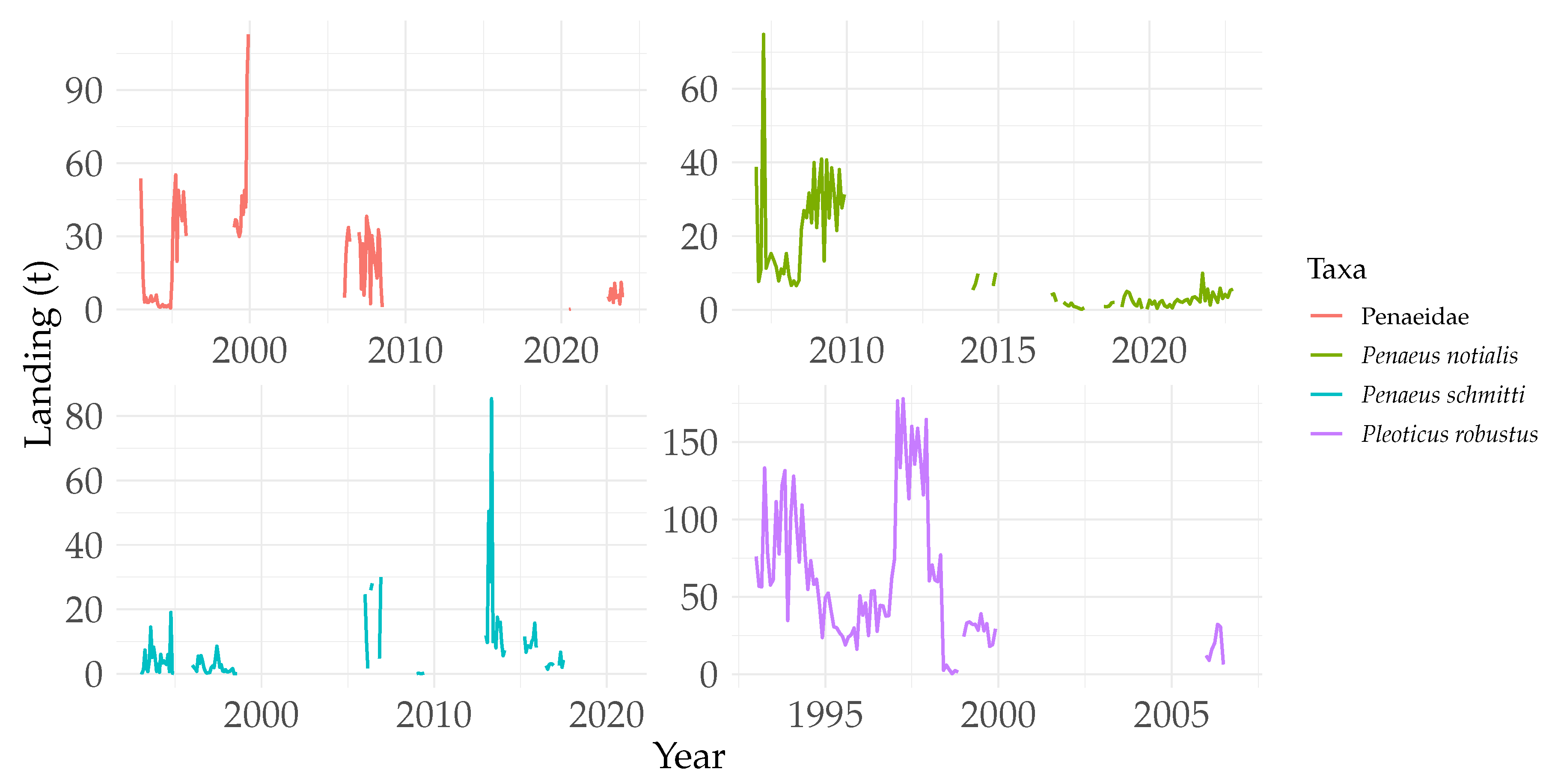
Figure 5.
Comparative distribution (median, interquartile range, and outliers) of landing across taxa.
Figure 5.
Comparative distribution (median, interquartile range, and outliers) of landing across taxa.
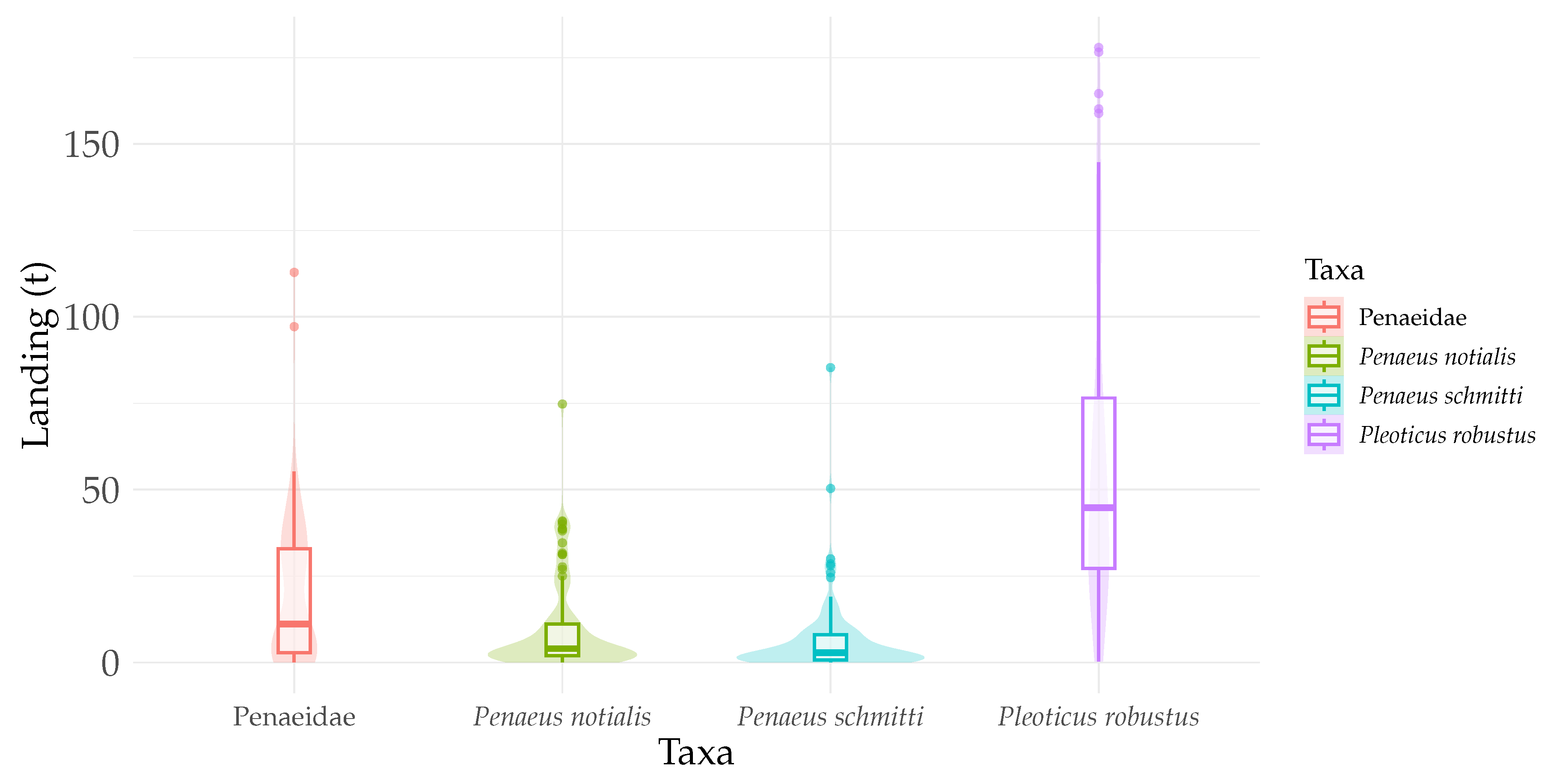
Figure 6.
Fully reconstructed historical landing time series (1993–2023) generated via non-parametric Random Forest imputation (missForest).
Figure 6.
Fully reconstructed historical landing time series (1993–2023) generated via non-parametric Random Forest imputation (missForest).
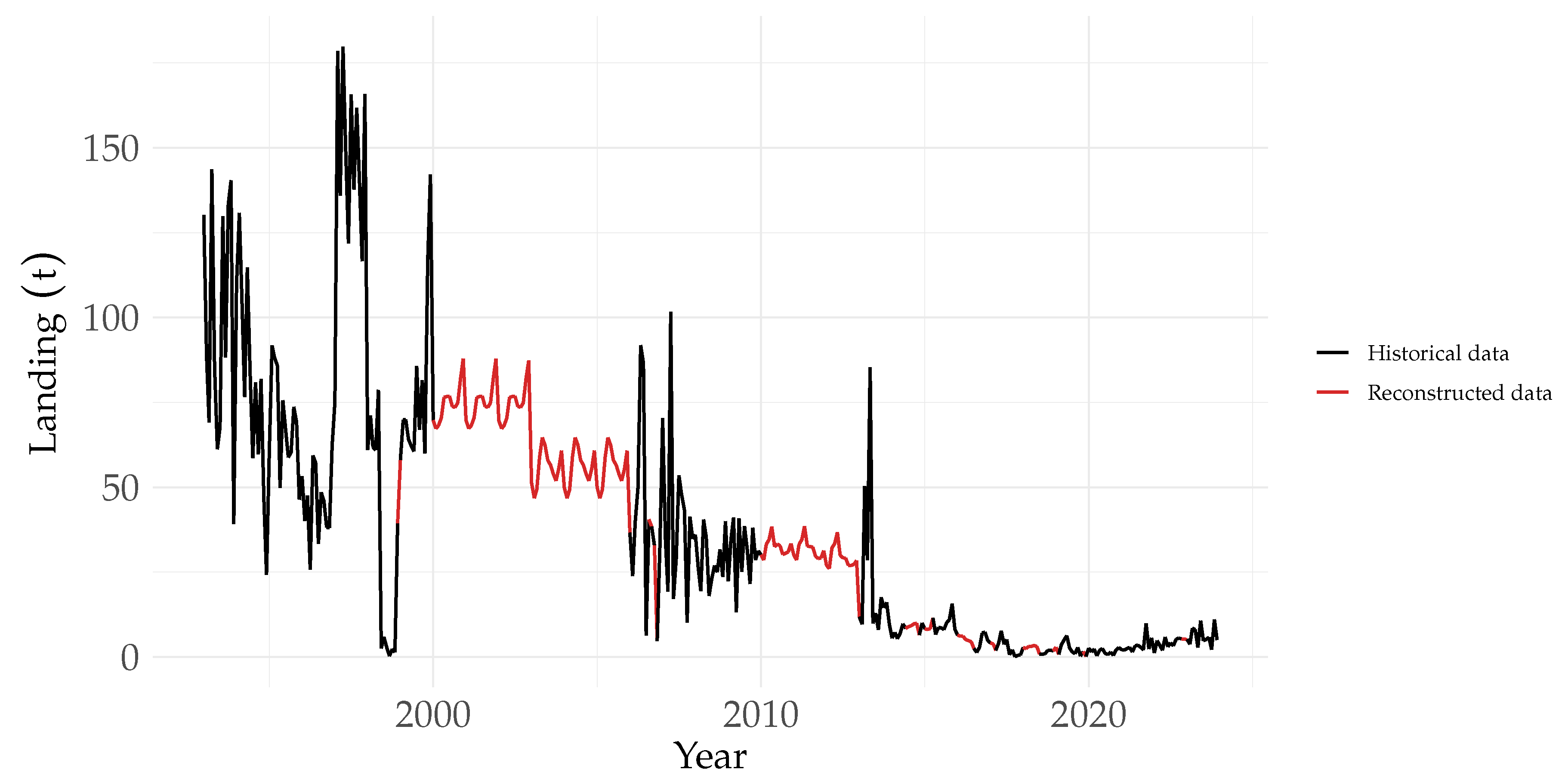
Figure 7.
Comparative longitudinal trajectories of predicted landings (t) across candidate models.
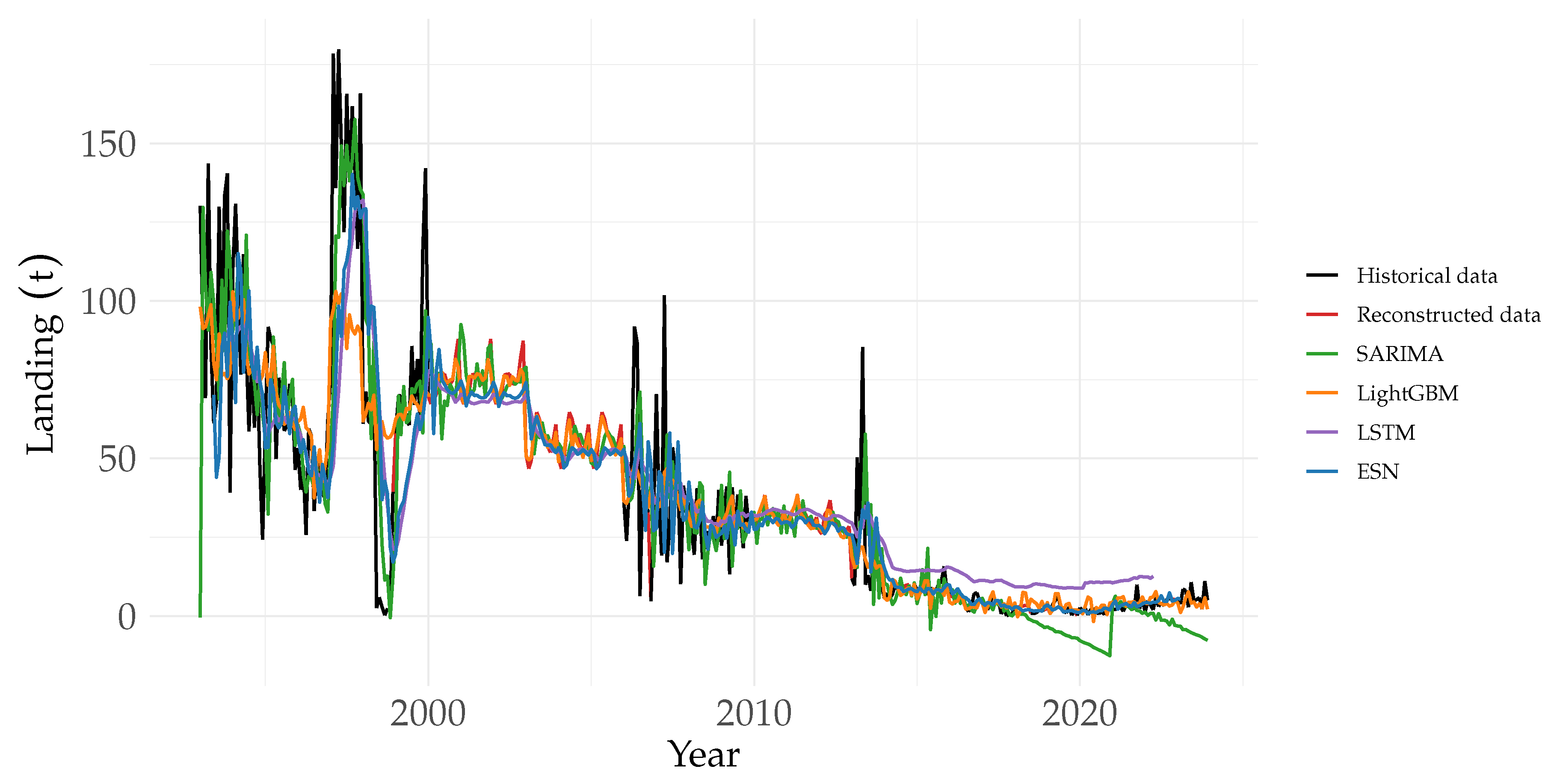
Figure 8.
Reconstructed landing time series using the ESN model with soft temporal weighting (forecasting/backcasting) alongside and confidence intervals.
Figure 8.
Reconstructed landing time series using the ESN model with soft temporal weighting (forecasting/backcasting) alongside and confidence intervals.
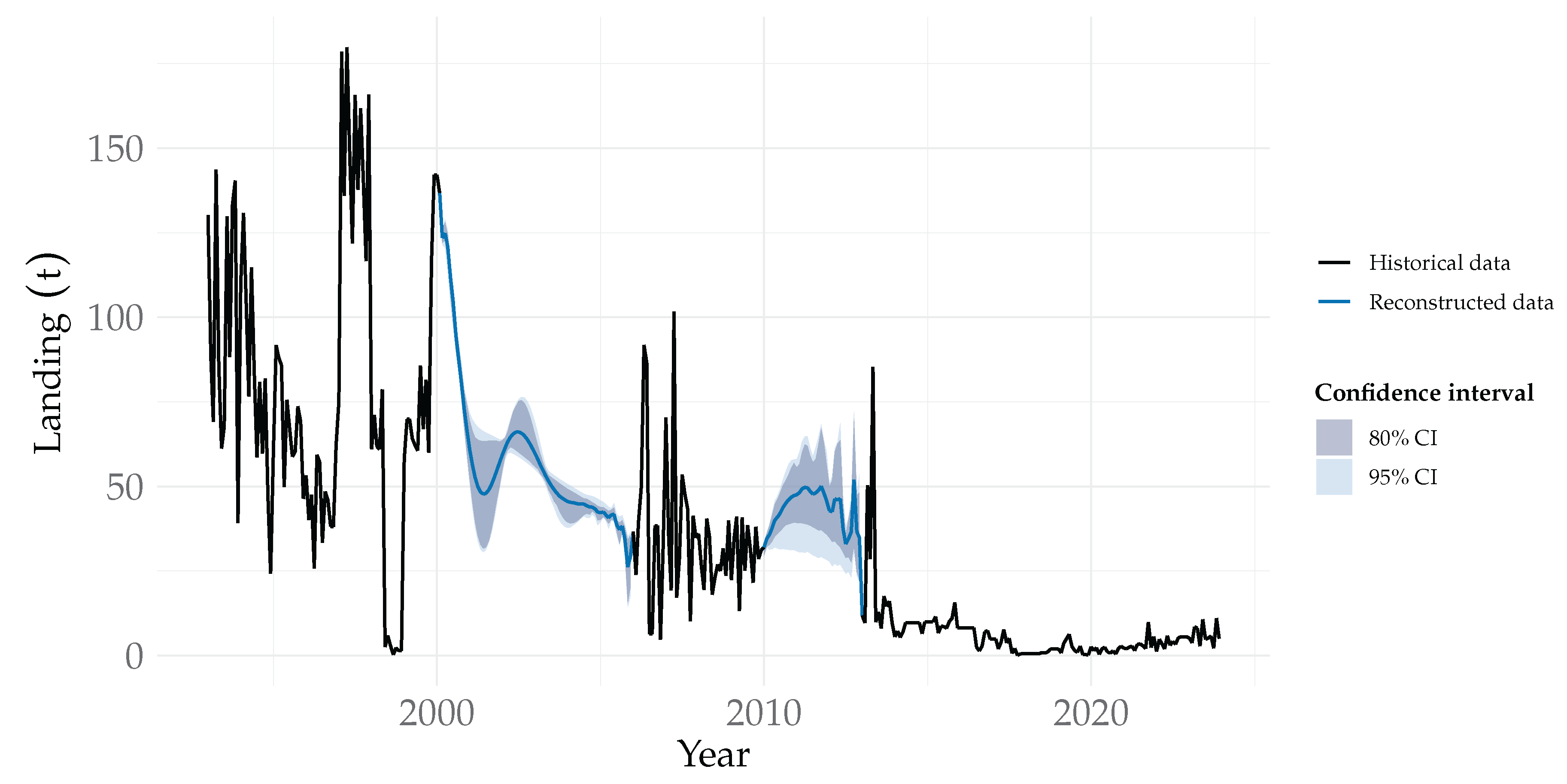

Table 1.
Statistical summary of reported landings (t) for the overall fishery and key target taxa of the shallow-water shrimp (SWS) industrial trawl fleet in the Colombian Caribbean (1993–2023).
Table 1.
Statistical summary of reported landings (t) for the overall fishery and key target taxa of the shallow-water shrimp (SWS) industrial trawl fleet in the Colombian Caribbean (1993–2023).
| Variable | N | Valid | Min | Q1 | Median | Mean | Q3 | Max | Missing | Missing |
|---|---|---|---|---|---|---|---|---|---|---|
| Landings | 372 | 234 | 138 | |||||||
| Penaeus notialis | 144 | 103 | 41 | |||||||
| Penaeus schmitti | 168 | 109 | 59 | |||||||
| Penaeidae | 240 | 92 | 148 | |||||||
| Pleoticus robustus | 96 | 91 | 5 |
Table 2.
Descriptive statistics of the fully reconstructed 1993–2023 landing dataset (t) after missForest non-parametric imputation.
Table 2.
Descriptive statistics of the fully reconstructed 1993–2023 landing dataset (t) after missForest non-parametric imputation.
| Variable | N | Valid | Min | Q1 | Median | Mean | Q3 | Max |
|---|---|---|---|---|---|---|---|---|
| 372 | 372 |
Table 3.
Chronological data partitioning scheme for the 1993–2023 monthly reported landing time series ().
Table 3.
Chronological data partitioning scheme for the 1993–2023 monthly reported landing time series ().
| Data Split | Years | Proportion (%) | Observations (n) | Imputed observations (n) | Imputed observations (%) |
|---|---|---|---|---|---|
| Train | 1993–2017 | 300 | 127 | ||
| Validation | 2018–2020 | 36 | 9 | ||
| Test | 2021–2023 | 36 | 2 |
Table 4.
Statistical summary for the scenario across training, validation, and test splits (t).
| Scenario | Split | N | Valid | Min | Q1 | Median | Mean | Q3 | Max |
|---|---|---|---|---|---|---|---|---|---|
| Train | 300 | 300 | |||||||
| Val | 36 | 36 | |||||||
| Test | 36 | 36 |
Table 5.
Statistical summary of the landing subseries.
| Landing Series | N | Valid (n) | Min | Q1 | Median | Mean | Q3 | Max | Missing (n) | Missing (%) |
|---|---|---|---|---|---|---|---|---|---|---|
| 85 | 83 | 2 | ||||||||
| 48 | 46 | 2 | ||||||||
| 132 | 105 | 27 |
Table 6.
NVIDIA Jetson Orin Nano hardware and software specifications.
| Feature | Specification |
|---|---|
| GPU | 1024-core NVIDIA Ampere, 32 Tensor Cores |
| CPU | 6-core Arm Cortex-A78AE v8.2 @ up to 1.73 GHz |
| Memory | 8 GB LPDDR5 (Unified Architecture) |
| Storage | NVMe SSD |
| Power Profile | 7–15 W (15 W Mode Enabled) |
| Operating System | NVIDIA JetPack 6.2.3 (L4T R36.5.2, Ubuntu 22.04 LTS) |
| CUDA Toolkit | Version 12.6 (V12.6.68) |
| Execution Backend | JAX v0.5.2 (jax[cuda] acceleration) |
Table 7.
Structural hyperparameters and dynamic settings for the JAX-accelerated Echo State Network (ESN).
Table 7.
Structural hyperparameters and dynamic settings for the JAX-accelerated Echo State Network (ESN).
| Hyperparameter / Setting | Selected Value |
|---|---|
| Input Dimension / Lags () | 5 |
| Reservoir Size () | 500 |
| Spectral Radius () | |
| Leaking Rate () | |
| Reservoir Sparsity (s) | () |
| Input Scaling () | |
| Ridge Regularization () | () |
| Reservoir Activation Function | tanh |
| Transient Washout Period () | 200 steps |
| Initial Reservoir State () | Zero Vector () |
| Readout Optimization | Ridge Regression (Closed-Form) |
| Random Seed (PRNGKey) | 42 |
Hyperparameters optimized via temporal grid search evaluated on validation MSE according to Lukoševičius (2012) [50]. Implemented natively in JAX using 64-bit floating-point precision (float64) to ensure numerical stability during readout layer matrix inversion.
Table 8.
Parameter estimates and diagnostic statistics for the fitted model on the landing time series ().
Table 8.
Parameter estimates and diagnostic statistics for the fitted model on the landing time series ().
| Parameter | Coefficient | Std. Error |
|---|---|---|
| c | ||
| Model Fit Metrics: Log-Likelihood: AIC: BIC: HQIC: | ||
| Residual Diagnostics: Ljung-Box (); | ||
| Jarque-Bera (); Heteroskedasticity (). | ||
Table 9.
Optimal hyperparameter configuration and structural settings for the LightGBM gradient boosting model.
Table 9.
Optimal hyperparameter configuration and structural settings for the LightGBM gradient boosting model.
| Hyperparameter | Selected Value |
|---|---|
| Boosting Type | GBDT |
| Objective Function | regression_l1 (MAE) |
| Evaluation Metric | rmse |
| Number of Estimators (M) | 878 |
| Learning Rate () | |
| Maximum Tree Depth () | 9 |
| Number of Leaves () | 47 |
| Min. Child Samples () | 20 |
| Subsample Ratio () | |
| Feature Fraction () | |
| Regularization () | |
| Regularization () | |
| Random Seed | 42 |
Hyperparameters optimized via randomized search temporal cross-validation (TimeSeriesSplit, iterations). Early stopping was set to 100 rounds on the validation split. Parallel execution was configured using all available CPU threads (n_jobs = -1).
Table 10.
Architectural specifications and optimal hyperparameters for the LSTM benchmark model.
| Hyperparameter / Setting | Selected Value |
|---|---|
| Lookback Window / Timesteps (T) | 10 |
| Input Features () | 1 |
| LSTM Hidden Units (u) | 128 |
| LSTM Activation Function | ReLU |
| Dropout Rate () | |
| Output Layer Units () | 1 |
| Optimizer | Adam |
| Learning Rate () | |
| Loss Function | MSE |
| Evaluation Metric | RMSE |
| Batch Size (B) | 32 |
| Training Epochs (E) | 100 |
| Total Trainable Parameters () |
Hyperparameters were selected via random search ( trials evaluated on denormalized validation RMSE). Model weights were updated using Backpropagation Through Time (BPTT).
Table 11.
Performance evaluation metrics across models and dataset splits.
| Model | Split | MAE | RMSE | RMSSE | Inference Latency (ms/sample) | RAMpeak (MB) | Sys. RAM Usage (%) |
|---|---|---|---|---|---|---|---|
| SARIMA | Train | 0 | |||||
| Val | 0 | ||||||
| Test | 0 | ||||||
| LightGBM | Train | 0 | |||||
| Val | 0 | ||||||
| Test | 0 | ||||||
| LSTM | Train | ||||||
| Val | 0 | ||||||
| Test | 0 | ||||||
| ESN | Train | ||||||
| Val | 0 | ||||||
| Test | 0 |
Table 12.
Descriptive statistical properties and operational domain metrics of model predictions.
| Model | N | Valid | Min | Q1 | Median | Mean | Q3 | Max | Missing | Missing |
|---|---|---|---|---|---|---|---|---|---|---|
| SARIMA | 372 | 372 | 0 | 0 | ||||||
| LightGBM | 372 | 372 | 0 | 0 | ||||||
| LSTM | 342 | 342 | 0 | 0 | ||||||
| ESN | 357 | 357 | 0 | 0 |
Table 13.
Walk-Forward Validation metrics across models.
| Model | MAE | RMSE | RMSSE | Total Time (s) | Inference Latency () | RAMWFV (MB) | Sys. RAM Usage (%) | Avg. Power (W) | Min. Power (W) | Max. Power (W) |
|---|---|---|---|---|---|---|---|---|---|---|
| SARIMA | ||||||||||
| LightGBM | ||||||||||
| LSTM | ||||||||||
| ESN |
Table 14.
Statistical summary of the observed landing series and the confidence intervals (80% and 95%) generated by the ESN during the reconstruction stages.
Table 14.
Statistical summary of the observed landing series and the confidence intervals (80% and 95%) generated by the ESN during the reconstruction stages.
| Variable | Valid (n) | Min | Q1 | Median | Mean | Q3 | Max |
|---|---|---|---|---|---|---|---|
| 372 | |||||||
| 107 | |||||||
| 107 | |||||||
| 107 | |||||||
| 107 |
Table 15.
Walk-Forward Validation performance metrics and dispersion analysis across 10 random seed initializations ().
Table 15.
Walk-Forward Validation performance metrics and dispersion analysis across 10 random seed initializations ().
| Metric | Mean | Standard Deviation | Minimum | Maximum |
|---|---|---|---|---|
| MAE | ||||
| RMSE | ||||
| RMSSE |
Disclaimer/Publisher’s Note: The statements, opinions and data contained in all publications are solely those of the individual author(s) and contributor(s) and not of MDPI and/or the editor(s). MDPI and/or the editor(s) disclaim responsibility for any injury to people or property resulting from any ideas, methods, instructions or products referred to in the content. |
© 2026 by the authors. Licensee MDPI, Basel, Switzerland. This article is an open access article distributed under the terms and conditions of the Creative Commons Attribution (CC BY) license.
Copyright: This open access article is published under a Creative Commons CC BY 4.0 license, which permit the free download, distribution, and reuse, provided that the author and preprint are cited in any reuse.