Preprint
Article

This version is not peer-reviewed.

Persistent Hypereutrophy and Limited One-Month-Ahead Forecastability in the Inner Bay of Lake Titicaca: Change-Point Analysis and Leakage-Aware Temporal Validation

Submitted:

26 August 2026

Posted:

27 August 2026

You are already at the latest version

Abstract

High-altitude lakes are increasingly exposed to nutrient enrichment, organic loading and wastewater-derived contamination, while predictive performance can be overstated when temporally ordered observations are randomly partitioned or target-defining measurements are reused as predictors. We analyzed 177 consecutive monthly water-quality records from the Inner Bay of Lake Titicaca, Peru (January 2011–September 2025), integrating Carlson’s composite trophic state index (CTSI), Hamed–Rao modified Mann–Kendall tests, block-bootstrap Sen slopes, Pettitt change-point detection with 12-month block permutation, nutrient stoichiometry, correlation, principal component analysis, leakage-aware contemporaneous classification and one-month-ahead forecasting. Total phosphorus was treated as elemental P and phosphate as PO4. The bay remained chronically hypereutrophic (mean CTSI 74.08 ± 4.07; 83.1% of months). BOD5 increased by 0.548 mg L−1 yr−1, chlorophyll a by 3.254 mg m−3 yr−1, total suspended solids by 0.752 mg L−1 yr−1 and conductivity by 13.13 µS cm−1 yr−1, whereas total phosphorus declined by 0.085 mg P L−1 yr−1. Block-supported shifts occurred in chlorophyll-a in November 2016 (21.81 to 54.18 mg m−3) and BOD5 in June 2018 (6.54 to 11.77 mg L−1). After removing target-defining variables and preserving temporal order, the best trophic-state classifier had balanced accuracy 0.575 and MCC 0.257. Organic-pollution classification had balanced accuracy 0.624 but sensitivity only 0.271, whereas the fecal-indicator model was unstable (MCC 0.130; ROC-AUC 0.460). Persistence was the best BOD5 forecast (RMSE 4.193 mg L−1; R² 0.390). The best CTSI model explained only 4.8% of future variance, and all thermotolerant-coliform forecasts had negative out-of-time R². Persistent ecological degradation was therefore evident, but monthly observations alone were insufficient for deployment-ready early warning. Higher-frequency sensing, hydrometeorological and wastewater-load covariates, spatial replication, direct microbiological measurements and prospective validation are required.

Keywords: 
;  ;  ;  ;  ;  ;  

1. Introduction

Freshwater ecosystems support biodiversity, food production, drinking-water supply, fisheries, recreation and cultural livelihoods, but they are increasingly altered by urbanization, land-use change, modified hydrology and climate warming (Albert et al., 2021; Reid et al., 2019; Tickner et al., 2020). Eutrophication remains one of the most persistent forms of degradation because excessive nitrogen and phosphorus stimulate phytoplankton production, reduce transparency, increase organic-matter accumulation and disrupt oxygen dynamics (Carpenter et al., 1998; Paerl & Otten, 2013; Smith & Schindler, 2009; Song et al., 2023). Robust diagnosis should integrate pollutant pressures, nutrient pathways, physicochemical state and biological responses rather than rely on a single nutrient concentration or composite index (Suresh et al., 2023). In shallow systems, external loading interacts with sediment recycling, resuspension, residence time and food-web processes, so a decline in one measured nutrient does not necessarily indicate ecological recovery (Conley et al., 2009; Kowalczewska-Madura et al., 2022; Schindler, 2006).
Tropical high-altitude lakes are particularly sensitive. Reduced atmospheric pressure modifies gas solubility, intense solar radiation affects biological production, large diel temperature ranges alter mixing and metabolism, and concentrated wet-season inflows can rapidly change nutrient and microbial loads (Adrian et al., 2009; Moser et al., 2019; Woolway et al., 2020). Recent Lake Titicaca research has documented taxonomic turnover and biodiversity loss in phytoplankton and periphyton along anthropogenic eutrophication gradients (Lanza et al., 2024). These conditions complicate interpretation of dissolved oxygen: high daytime concentrations may reflect photosynthetic supersaturation, while nighttime respiration and decomposition can still create oxygen stress. Monthly daytime sampling may therefore mask ecologically important deoxygenation and diel variability (Jansen et al., 2024; Liu et al., 2025).
Lake Titicaca lies at approximately 3810 m above sea level on the Peruvian–Bolivian Altiplano and sustains fisheries, navigation, tourism, urban water uses and culturally important livelihoods. Its Inner Bay of Puno is shallow and semi-enclosed, with restricted exchange with the open lake. Morphobathymetric studies describe an area of about 16.1 km², a mean depth near 2.7 m and a maximum depth of approximately 7.4 m (Loza del Carpio et al., 2016; Dejoux & Iltis, 1992; Northcote et al., 1991). Recent basin studies have quantified elevated BOD5, nitrogen, phosphorus, suspended-solids and fecal-indicator inputs from tributaries and wastewater discharges in the Peruvian sector, while stable-isotope evidence from the Bolivian sector has traced anthropogenic carbon and nitrogen incorporation away from wastewater sources (Heredia et al., 2022; Siguayro et al., 2022). Together with documented biological turnover and water-quality impairment, these findings confirm that urban growth, insufficient wastewater treatment, diffuse runoff and legacy sediment enrichment are basin-wide pressures (Farfán et al., 2015; Flores-Gómez et al., 2024; Lanza et al., 2024).
Long monitoring records are essential for distinguishing chronic impairment, gradual deterioration, abrupt statistical shifts and genuine recovery. Conventional trend tests are robust to non-normality, but serial dependence can inflate inferential certainty (Hirsch et al., 1982). Modified Mann–Kendall procedures and block resampling provide more defensible inference when observations are autocorrelated (Hamed & Rao, 1998; Künsch, 1989; Yue et al., 2002). Change-point analysis complements monotonic trends by identifying dates at which a series shifts, although such dates do not by themselves establish ecological causation. Multivariate analyses can further determine whether degradation is dominated by one common gradient or by partially independent trophic, organic, ionic and microbiological processes.
Machine learning is increasingly used in environmental assessment because nonlinear models can represent complex interactions (Olden et al., 2008; Reichstein et al., 2019). Recent water-quality studies show that useful prediction depends not only on algorithm choice but also on informative covariates, high-frequency observations, appropriate spatiotemporal design and rigorous evaluation against future observations (Del Castillo et al., 2024; Grbčić et al., 2022; Pandit et al., 2025; Zhu et al., 2022). Applications remain vulnerable to target leakage, random cross-validation of temporally ordered data and reliance on accuracy under class imbalance (Kapoor & Narayanan, 2023; Kaufman et al., 2012; Roberts et al., 2017). Recent work also shows that apparently similar predictive performance can conceal unstable model explanations and sensitivity to data splitting (Panigrahi et al., 2025). MCC, balanced accuracy and precision–recall metrics are therefore more informative than raw accuracy alone (Chicco & Jurman, 2020; Saito & Rehmsmeier, 2015).
This study integrated long-term ecological assessment with a transparent audit of predictive validity. The objectives were to: (1) characterize trophic, organic and microbiological conditions in the Inner Bay from 2011 to 2025; (2) estimate autocorrelation-robust long-term changes and identify abrupt statistical shifts; (3) examine nutrient stoichiometry, correlation structure and multivariate organization; (4) quantify how leakage-aware temporal validation changes contemporaneous classification performance; and (5) compare seven machine-learning algorithms with persistence in genuine one-month-ahead forecasts of CTSI, BOD5 and thermotolerant coliforms. We hypothesized that chronic hypereutrophy would coexist with worsening organic pollution and that models evaluated without temporal or target leakage would generalize substantially less well than leakage-prone models.

2. Materials and Methods

2.1. Study Area and Monitoring Record

The Inner Bay of Puno is located on the western margin of Lake Titicaca, Peru (approximately 15°50′–15°53′ S; 69°59′–70°02′ W). It is a shallow, semi-enclosed basin connected to the main lake through a narrow channel. Restricted exchange and prolonged effective residence time favor the accumulation and recycling of dissolved and particulate pollutants. The regional climate has a concentrated rainy period and a prolonged dry season, which influence runoff, tributary inflow, suspended solids and microbiological transport.
Monthly observations were obtained from the long-term monitoring program of the Instituto del Mar del Perú (IMARPE) for January 2011–September 2025. The analytical series contained 177 consecutive monthly records and 17 variables: surface-water temperature, electrical conductivity, total suspended solids (TSS), Secchi depth, dissolved oxygen (DO), pH, chlorophyll-a, chemical oxygen demand (COD), 5-day biochemical oxygen demand (BOD5), nitrite, nitrate, phosphate, total nitrogen (TN), total phosphorus (TP), ammonium/ammonia, total coliforms and thermotolerant coliforms (TTC). The dataset was treated as one continuous aggregated monitoring series. Complete institutional metadata on station composition, sampling depth, analytical method, detection limit and aggregation procedures were not available; possible changes in those elements were therefore treated as structural uncertainty.

2.2. Quality Control, Chemical Basis and Derived Indicators

Dates were parsed and sorted chronologically. Units, duplicated dates, impossible values and non-positive concentrations required by logarithmic formulas were checked. The analytical table contained no missing values, so imputation was not performed. Extreme values were retained when compatible with plausible pollution events; no observation was removed solely because it was statistically unusual. Based on the confirmed reporting basis supplied for this revision, total phosphorus was interpreted as elemental phosphorus (mg P L−1), total nitrogen as elemental nitrogen (mg N L−1), and phosphate as the phosphate ion PO4 (mg PO4 L−1). Phosphate was not converted to P and was not used in the TN:TP ratio.
Carlson’s trophic-state components were calculated as TSI(Chl-a) = 9.81 ln(Chl-a) + 30.6, TSI(SD) = 60 − 14.41 ln(SD), and TSI(TP) = 14.42 ln(TP in µg P L−1) + 4.15 (Carlson, 1977). CTSI was their arithmetic mean. Monthly states were categorized as eutrophic (50 to <70) or hypereutrophic (≥70); no observations fell in lower categories. For descriptive comparison, TP was evaluated against 0.035 mg P L−1, the Category 4–E1 lake benchmark in Peru’s DS 004-2017-MINAM. BOD5 >10 mg L−1 was prespecified as a severe organic-load screen (twice the Category 4–E1 benchmark), and TTC ≥200 MPN 100 mL−1 was used as a primary-contact screening threshold. These screens were used for description and model auditing only; they are not presented as formal legal non-compliance because the applicable designated use and official water-body assignment were not independently verified (Ministerio del Ambiente del Perú, 2017).
Molar TN:TP was calculated as (TN/14.0067)/(TP/30.9738). Ratios <10, 10–20 and >20 were treated as exploratory indicators of potential nitrogen limitation, co-limitation and phosphorus limitation, respectively (Guildford & Hecky, 2000). These categories do not demonstrate nutrient limitation; enrichment bioassays and chemical-speciation data are required for confirmation.

2.3. Descriptive Statistics, Robust Trends and Change Points

Each variable was summarized by its mean, standard deviation, median, minimum and maximum. Monotonic change was described with Kendall’s tau and Sen’s slope, converted to annual units. Because several series were strongly autocorrelated, significance was based primarily on the Hamed–Rao modified Mann–Kendall test, with trend-free prewhitening as a sensitivity analysis (Hamed & Rao, 1998; Yue et al., 2002). Ninety-five percent confidence intervals for annual Sen slopes were estimated using a circular moving-block bootstrap with 12-month blocks and 1,200 resamples, preserving within-year dependence (Künsch, 1989). Lag-1 autocorrelation (ACF1) was reported as a diagnostic. A 12-month block length was selected to preserve potential annual seasonal dependence in the monthly monitoring series
Abrupt shifts were evaluated with Pettitt’s non-parametric single-change-point test (Pettitt, 1979). To reduce false certainty from serial dependence, conventional Pettitt probabilities were supplemented with 999 permutations of intact 12-month blocks. Pre- and post-change means were reported. A change-point date identifies the most likely statistical break in a series; it does not prove an ecological regime shift, management effect or causal mechanism.

2.4. Association and Multivariate Structure

Spearman correlations described monotonic associations among trophic, nutrient, organic-pollution and microbiological indicators. Correlations between CTSI and its components, and between TN:TP and its numerator or denominator, were interpreted as partly mathematical rather than independent ecological evidence. Principal component analysis (PCA) was performed on standardized environmental variables; total and thermotolerant coliforms were log1p-transformed before standardization. Explained variance, eigenvalues and loadings were inspected. PCA was interpreted as exploratory ordination rather than a causal model.

2.5. Leakage-Aware Contemporaneous Classification

Three binary classification tasks were evaluated: hypereutrophic versus eutrophic state, BOD5 >10 versus ≤10 mg L−1, and TTC ≥200 versus <200 MPN 100 mL−1. The positive class was the higher-risk state in every task. Logistic regression, random forest and radial-basis support-vector machine classifiers were compared. To prevent direct target leakage, chlorophyll-a, TP and Secchi depth were excluded from the trophic-state model; BOD5 was excluded from the organic-pollution model; and TTC was excluded from the fecal-indicator model. Total coliforms were retained as a related but distinct contemporaneous measurement.
The primary evaluation used four prespecified expanding windows: 2018–2019, 2020–2021, 2022–2023 and January 2024–September 2025, each tested only after training on all preceding observations. Exact fold dates and event counts are provided in Table S1. Scaling and all learned preprocessing were fitted within training data only. Hyperparameters were fixed a priori (Table S5), avoiding tuning on future observations. Out-of-fold predictions were pooled across the 93 evaluation months. Metrics included accuracy, balanced accuracy, macro-F1, MCC, sensitivity, specificity, positive predictive value, PR-AUC and ROC-AUC. Six-month circular block-bootstrap intervals (400 resamples) quantified uncertainty. A separate five-fold random analysis retaining target-defining measurements was used only to illustrate leakage inflation and was not treated as a valid prediction.

2.6. One-Month-Ahead Forecasting

CTSI, BOD5 and TTC values were forecast one month ahead. Predictors consisted only of information available before the target month: one- and two-month lags of the 17 monitored variables and CTSI, plus sine and cosine terms for month of year. Previous target observations were retained only as lagged predictors available at the forecast origin; no contemporaneous or future target measurement entered the feature matrix. TTC was transformed with log(1+x) to reduce right skew.
Seven algorithms were compared: ridge regression, elastic net, random forest, extremely randomized trees, gradient boosting, support-vector regression with a radial basis kernel and XGBoost (Friedman, 2001; Zou & Hastie, 2005; Geurts et al., 2006; Chen & Guestrin, 2016). Persistence, defined as the previous month’s observed value on the evaluation scale, was the mandatory benchmark. The same four expanding windows were used. Performance was summarized by pooled out-of-time RMSE, MAE and R². Six-month circular block-bootstrap intervals (300 resamples) were calculated for each metric and for the difference in RMSE relative to persistence. A learned model was considered potentially useful only if it achieved positive out-of-time R² and a consistent RMSE improvement over persistence.

2.7. Software, Transparency and Reproducibility
Analyses were conducted in Python using pandas, NumPy, SciPy, scikit-learn, pymannkendall, XGBoost and matplotlib. A fixed seed (20260711) was used where algorithms required stochastic initialization. The submission package should include the de-identified analytical dataset where authorization permits, a data dictionary, software versions, fold dates, preprocessing steps, code, random seeds and the hyperparameters listed in Table S5. No ARIMA, ETS or other autoregressive statistical forecasting model was used.
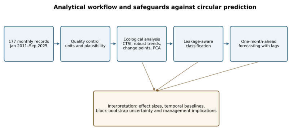
Figure 1. Analytical workflow. Trend inference used autocorrelation-aware tests and block resampling; classification excluded target-defining contemporaneous variables; forecasting used only lagged information available before the target month. 
Preprints 230178 g001

3. Results

3.1. Water-Quality Characteristics and Trophic State

The 177-month record showed a persistent high-productivity state and marked variability in pollution indicators (Table 1). Mean chlorophyll-a was 41.20 mg m−3, mean Secchi depth was 1.31 m, mean pH was 9.30 and mean DO was 9.67 mg L−1. The combination of elevated phytoplankton biomass, low transparency, alkaline conditions and periods of oxygen supersaturation is consistent with intense daytime primary production rather than ecological recovery.
Mean CTSI was 74.08 ± 4.07, and 147 of 177 months (83.1%) were hypereutrophic. BOD5 exceeded 10 mg L−1 in 28.8% of observations and COD exceeded 30 mg L−1 in 48.6%. TTC reached or exceeded 200 MPN 100 mL−1 in 5.6% of months, while total coliforms exceeded 1000 MPN 100 mL−1 in 20.3%. TP exceeded the Category 4–E1 reference value of 0.035 mg P L−1 in every observation. These frequencies are descriptive and are not presented as a formal compliance determination.
Mean molar TN:TP was 8.98 and the median was 6.33. Because TN was expressed as N and TP as P, the atomic-weight conversion was directly applicable. In total, 74.0% of months had TN:TP <10, 15.3% were between 10 and 20, and 10.7% exceeded 20. The distribution is compatible with frequent nitrogen limitation or N–P co-limitation under persistent phosphorus enrichment, but requires experimental confirmation.

3.2. Long-Term Trends and Serial Dependence

BOD5 showed the strongest positive association with time (τ = 0.487), increasing by 0.548 mg L−1 yr−1 (12-month block-bootstrap 95% CI 0.353–0.744; Hamed–Rao p <0.001). Chlorophyll-a increased by 3.254 mg m−3 yr−1, TSS by 0.752 mg L−1 yr−1, conductivity by 13.13 µS cm−1 yr−1, DO by 0.218 mg L−1 yr−1 and nitrite by 0.012 mg L−1 yr−1. Total phosphorus declined by 0.085 mg P L−1 yr−1 (95% CI −0.133 to −0.040; adjusted p = 0.006). CTSI, COD and TTC did not show robust monotonic trends (Table 2; Figure 2).
Serial dependence was substantial for conductivity (ACF1 = 0.87), TP (0.82) and BOD5 (0.73). Despite wider block-bootstrap intervals and adjusted tests, the directions of the BOD5, chlorophyll-a, TSS, conductivity, DO, nitrite and TP trends remained supported. Increasing DO was interpreted jointly with increasing chlorophyll-a and pH, consistent with daytime photosynthetic supersaturation.

3.3 Abrupt Statistical Shifts

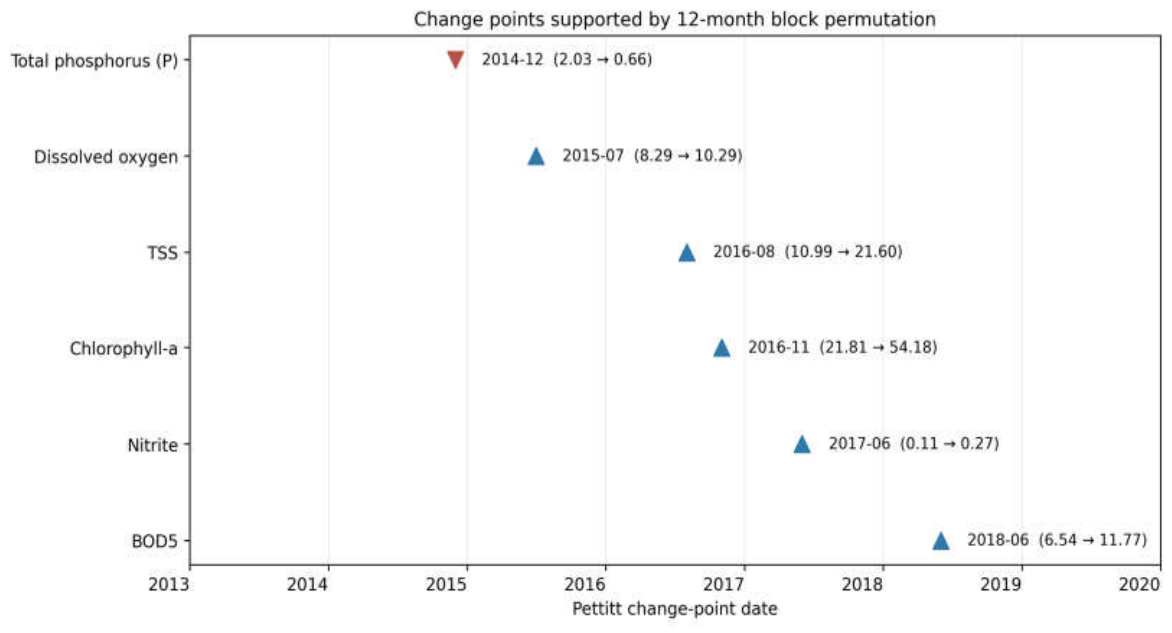
The Pettitt analysis identified several conventional shifts, but only six remained supported after permutation of intact 12-month blocks (Table 3; Figure 3). The clearest ecological changes were a rise in mean chlorophyll-a from 21.81 to 54.18 mg m−3 after November 2016 and a rise in mean BOD5 from 6.54 to 11.77 mg L−1 after June 2018. TSS, DO and nitrite also shifted upward, whereas TP shifted downward after December 2014.

3.4. Correlation and Multivariate Structure

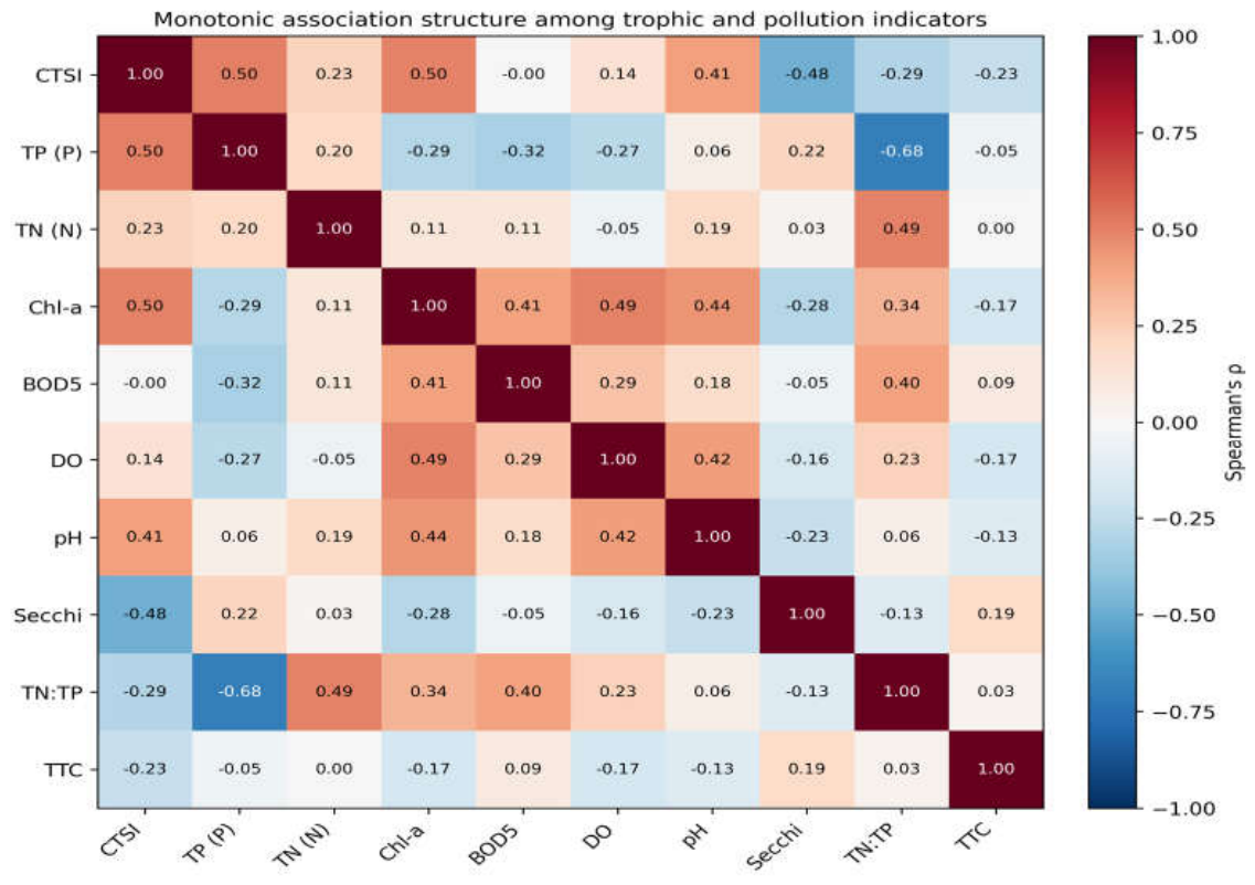
CTSI was positively associated with TP (ρ = 0.50), chlorophyll-a (ρ = 0.50) and pH (ρ = 0.41), and negatively associated with Secchi depth (ρ = −0.48) (Figure 4). Because TP, chlorophyll-a, and Secchi depth directly construct CTSI, these coefficients demonstrate internal consistency rather than independent prediction. Chlorophyll-a was associated with DO (ρ = 0.49), pH (ρ = 0.44), and BOD5 (ρ = 0.41), supporting a coupled pattern of production, organic- matter accumulation and daytime oxygen supersaturation. TN:TP was negatively associated with TP (ρ = −0.68) and positively associated with TN (ρ = 0.49), relationships that are partly mathematical.
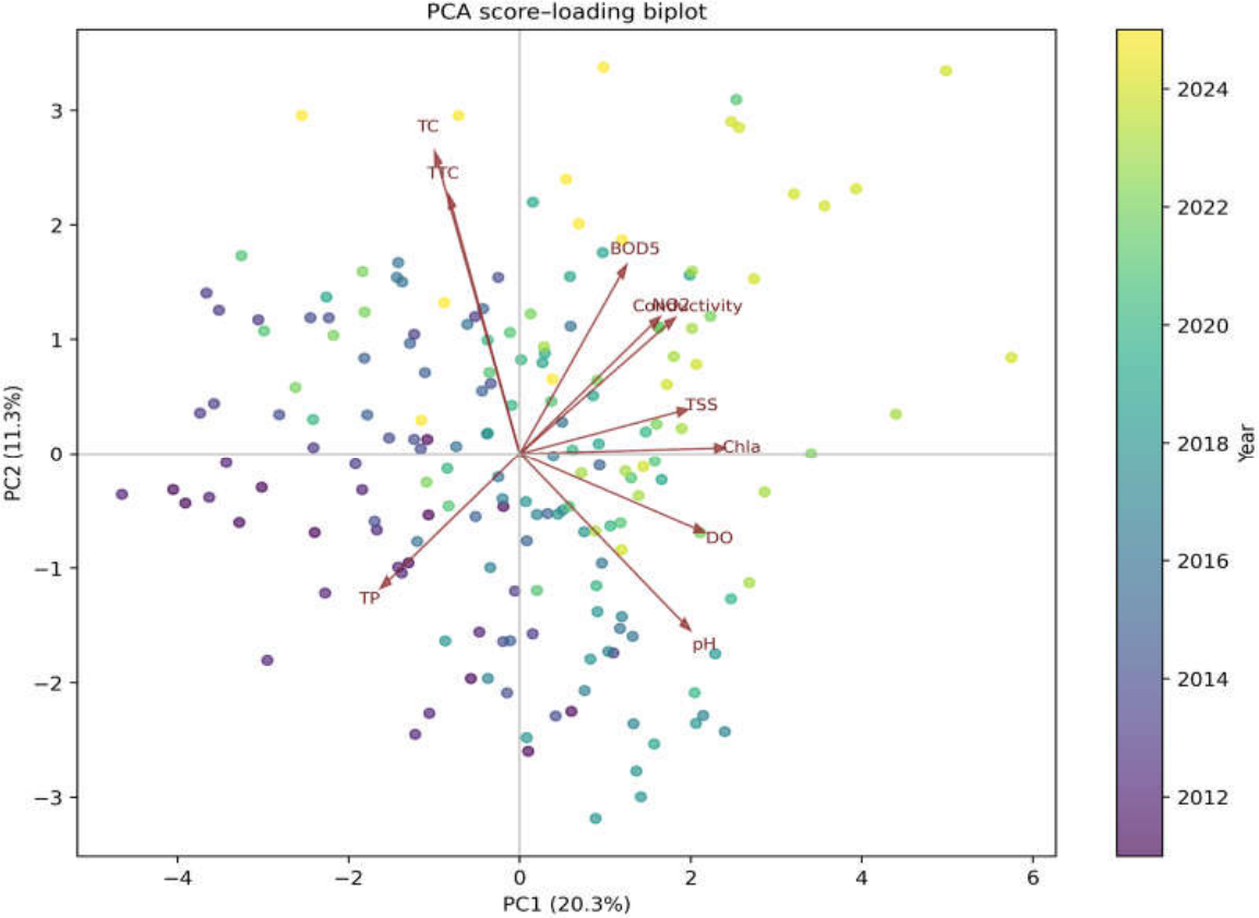
PCA did not reveal one dominant pollution axis. PC1 explained 20.3% of the variance and the first five components explained 56.4%. PC1 loaded positively on chlorophyll-a, DO, pH, TSS, conductivity and temperature and negatively on Secchi depth, TP and ammonium/ammonia. PC2 was dominated by total and thermotolerant coliforms. This diffuse structure indicates partially distinct trophic-production, organic, ionic, suspended-solid and microbiological signals. Detailed loadings and the score–loading biplot are provided in Table S2 and Figure S1.

3.5. Leakage-Aware Contemporaneous Classification

In the deliberately leakage-prone random analysis, retaining target-defining measurements produced ROC-AUC values of 0.940 for trophic state, 1.000 for organic pollution and 0.999 for fecal-indicator events. These values represent circular reconstruction and were not treated as valid predictive performance. Removing target-defining variables and preserving temporal order reduced performance substantially (Table 4).
For trophic-state classification, random forest achieved ROC-AUC 0.741 and PR-AUC 0.906, but balanced accuracy was only 0.575 and specificity for the eutrophic class was 0.176. Accuracy (0.828) was only marginally above the evaluation-set majority baseline (0.817), indicating that the model largely reproduced the dominant hypereutrophic state. Organic-pollution classification had balanced accuracy 0.624 and MCC 0.347, but sensitivity was only 0.271: it identified 13 of 48 high-BOD5 months while producing one false positive. The fecal-indicator model was unstable because only eight positive events occurred in the evaluation period; its MCC was 0.130, ROC-AUC was 0.460 and the confidence intervals included no discrimination. Direct microbiological measurement cannot be replaced by the available physicochemical variables. Table S3 provides results for every classifier and confusion matrix.

3.6. One-Month-Ahead Forecasting

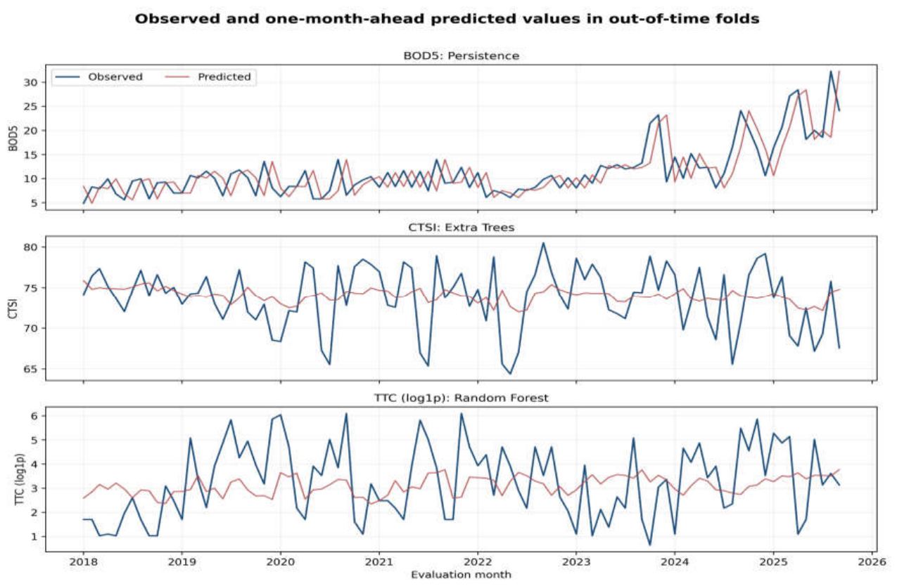
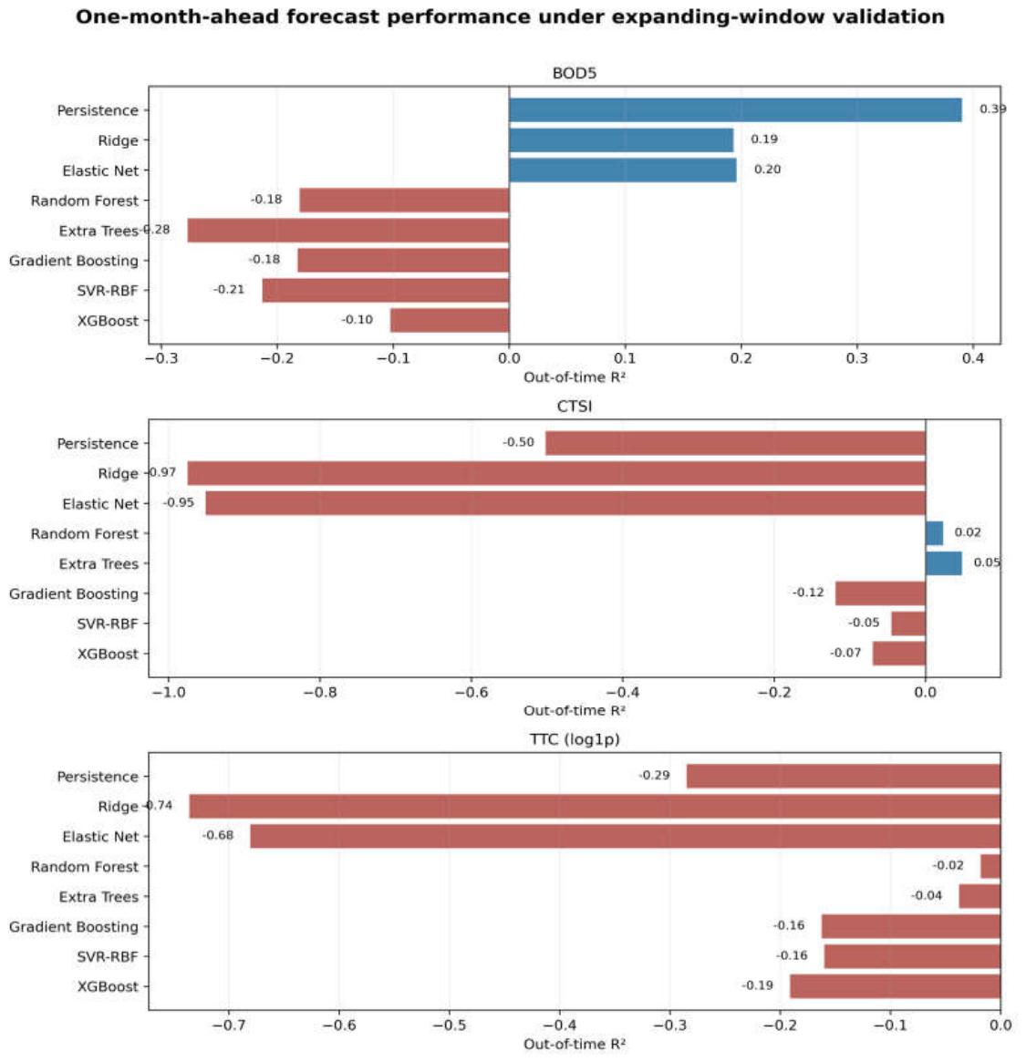
The forecasting experiment provided a direct assessment of prospective usefulness (Table 5; Figure 5). For BOD5, persistence was the strongest model (RMSE 4.193 mg L−1; MAE 3.213 mg L−1; R² 0.390). Elastic net was the best learned alternative (RMSE 4.816 mg L−1; R² 0.196), but its RMSE was 0.622 mg L−1 higher than persistence, with a block-bootstrap interval spanning a small improvement and substantial deterioration.
For CTSI, Extra Trees improved RMSE relative to persistence (3.733 versus 4.689 index units), but explained only 4.8% of future variance and its R² interval included zero (−0.044 to 0.126). For TTC on the log1p scale, random forest had the lowest RMSE (1.526) but negative R² (−0.018); its apparent RMSE improvement over persistence was also uncertain. Thus, no target met a deployment-ready criterion combining positive and stable out-of-time R² with reliable improvement over the benchmark.

4. Discussion

4.1. Persistent Hypereutrophy and Divergent Indicators

The principal ecological finding is not a progressive increase in CTSI but the persistence of a severely degraded state. CTSI averaged 74.08 and 83.1% of observations were hypereutrophic. In a compressed high-state distribution, absence of a monotonic CTSI trend does not indicate recovery; it indicates that the system remained predominantly within the same impaired category while its components changed in different directions. This interpretation is consistent with historical evidence from the Inner Bay and with recent Lake Titicaca studies showing wastewater-derived nutrient signals, elevated pollutant inputs, biological turnover and reduced algal community diversity along eutrophication gradients (Beltrán Farfán et al., 2015; Heredia et al., 2022; Siguayro et al., 2022; Lanza et al., 2024; Flores-Gómez et al., 2024).
The increases in chlorophyll-a, BOD5, and TSS provide stronger evidence of deterioration than the composite index alone. Higher chlorophyll-a indicates greater phytoplankton biomass, rising BOD5 indicates greater biodegradable organic load or decomposition demand, and increasing TSS can reduce transparency while enhancing resuspension of nutrient-rich material. Increasing conductivity suggests accumulating dissolved ionic inputs. These trajectories describe multidimensional degradation rather than a single nutrient-response relationship, consistent with integrated eutrophication frameworks (Suresh et al., 2023; Tammeorg et al., 2024). The fact that these conclusions survived autocorrelation adjustment and block-bootstrap uncertainty strengthens their interpretation.
High DO should not be read as improved ecological condition. Its positive association with chlorophyll-a and pH is consistent with intense daytime photosynthesis and CO2 depletion. Monthly daytime measurements can miss nocturnal oxygen minima, and high mean DO can coexist with strong diel amplitudes, sediment oxygen demand and episodic anoxia. High-frequency datasets now demonstrate how hourly observations reveal dynamics that fortnightly or monthly sampling cannot resolve (Eyring et al., 2025; Liu et al., 2025). Continuous oxygen saturation and temperature profiles are therefore required to evaluate metabolic stress and hypoxia risk.

4.2. Declining Phosphorus, Stoichiometry and Change Points

The decline in TP expressed as elemental P is counterintuitive because it occurred while chlorophyll-a and BOD5 increased and transparency remained low. Rapid biological uptake can lower surface-water concentrations while maintaining high biomass; legacy sediments can sustain effective phosphorus supply through redox-sensitive release and wind-driven resuspension; changing hydrology can alter concentration without lowering mass load; and undocumented changes in sampling or analytical practice can create an artificial break. Internal loading can remain spatially heterogeneous, event-driven and strongly coupled to oxygen, temperature and warming, delaying recovery after external-load reductions (Kowalczewska-Madura et al., 2022; Kong et al., 2023; Kirol et al., 2024; Tammeorg et al., 2024). The December 2014 TP shift therefore requires a metadata audit before it is interpreted as management success.
Block-aware change-point inference refined the earlier interpretation. The shifts in TP, DO, TSS, chlorophyll-a, nitrite and BOD5 remained supported, whereas the apparent changes in Secchi depth, phosphate, pH, total coliforms and conductivity did not survive 12-month block permutation. This distinction is important: conventional Pettitt probabilities can exaggerate evidence when serial dependence is ignored. The supported chronology still indicates a staged reorganization, but researchers should therefore treat these dates only as targets for metadata review and future sampling.
The predominance of TN:TP <10 is compatible with nitrogen limitation or N–P co-limitation under phosphorus-rich conditions. Because TN was reported as N and TP as P, the molar calculation is chemically coherent; PO4, reported as phosphate ion, was correctly excluded from the ratio. Ratios alone remain insufficient: seasonal N, P and N+P enrichment experiments, nutrient speciation and phytoplankton-community analysis are needed before a limiting nutrient is assigned (Redfield, 1958; Guildford & Hecky, 2000; Conley et al., 2009; Song et al., 2023).

4.3. What Leakage-Aware Validation Changes

The machine-learning audit is a central methodological contribution. Near-perfect discrimination occurred when predictors included measurements that directly defined the outcome. Such models reconstructed labels rather than predicting an independent environmental state. Removing target-defining measurements and preserving temporal order reduced performance sharply, demonstrating how leakage and random partitioning can create misleading claims in small environmental datasets (Kapoor & Narayanan, 2023; Kaufman et al., 2012; Roberts et al., 2017). This is especially relevant because recent environmental ML studies show that model behavior and explanations can vary with data splits and algorithm families even when headline performance appears similar (Panigrahi et al., 2025).
The corrected positive-class coding resolved the earlier inconsistency in the fecal-indicator metrics. The recalculated ROC-AUC of 0.460, MCC of 0.130 and very wide block-bootstrap intervals show that the task is not operationally useful. Trophic-state ranking was moderate, but threshold-level performance largely reflected the dominant hypereutrophic class. The organic-pollution classifier achieved high specificity but missed nearly three-quarters of high-BOD5 months. Reporting prevalence, confusion matrices, sensitivity, specificity, MCC, PR-AUC and uncertainty prevents one favorable metric from concealing these limitations (Chicco & Jurman, 2020; Saito & Rehmsmeier, 2015).
The one-month-ahead experiment was more stringent and more relevant to early warning. Persistence outperforming all learned BOD5 models shows that temporal continuity dominated the available information. Extra Trees produced a small positive CTSI R², but the interval included zero and the explained variance was too small for deployment. All TTC models had negative R². Complex algorithms therefore did not overcome missing process information, sparse microbiological events or temporal non-stationarity. Long hindcast evaluation and prospective forecasts, as used in operational harmful-algal-bloom systems, are necessary before deployment claims are justified (Liu et al., 2025). A scientifically honest weak or negative result is valuable because it prevents premature implementation and identifies the missing information needed to improve prediction.

4.4. Monitoring and Management Implications

Wastewater control remains the most defensible management priority. Treatment goals should extend beyond microbial removal to BOD5, ammonium, TN, TP and suspended solids. This priority is supported by substantial nutrient, organic and fecal-indicator inputs from tributaries and treatment-plant effluents around the Peruvian sector, together with isotope-traced anthropogenic enrichment elsewhere in the basin (Heredia et al., 2022; Siguayro et al., 2022). Because the present dataset contains concentrations rather than source-specific flows, it cannot quantify pollutant loads or attribute changes to individual discharges. Tributary flow, wastewater volume, treatment-plant performance and precipitation must be integrated to distinguish changes in loading from changes in dilution.
Internal loading may delay recovery after external inputs decline. Sediment oxygen demand, phosphorus release, organic-matter accumulation and resuspension should be measured alongside an external-load inventory, nutrient budget and hydrodynamic assessment. Restoration measures should be evaluated experimentally and adaptively rather than inferred from concentration trends alone (Kowalczewska-Madura et al., 2022; Kong et al., 2023; Kirol et al., 2024; Tammeorg et al., 2024).
A credible early-warning system should be designed prospectively. Continuous sensors for DO saturation, pH, temperature, conductivity, turbidity and chlorophyll fluorescence should be combined with laboratory nutrients and direct E. coli or thermotolerant-coliform enumeration. Rainfall, tributary discharge, lake level, wind, solar radiation and wastewater-operation variables are likely to supply the missing predictive information. High-frequency monitoring and process-informed environmental prediction increasingly demonstrate the value of temporal resolution and external drivers (Eyring et al., 2025; Pandit et al., 2025). Forecast horizons, thresholds and decision costs should be defined before model fitting; an untouched later period or a new monitoring station should then be used for external validation.

4.5. Strengths and Limitations

The main strengths are the unusually long monthly record for a tropical high-altitude bay, the joint analysis of trophic, organic and microbiological dimensions, autocorrelation-aware trend inference, block-aware change-point testing, explicit positive-class coding, fixed expanding windows and comparison with persistence. The separation between contemporaneous classification and genuine forecasting prevents complex models from being credited for information already contained in the target or in future observations.
The limitations are substantial. The analysis used a single aggregated monthly series and cannot resolve spatial heterogeneity. Monthly sampling masks diel oxygen dynamics and short-lived microbial pulses. Hydrometeorological variables, wastewater flows, cyanobacterial taxa and toxins, sediment fluxes and source-specific loads were unavailable. The 2025 record covered only January–September. Monitoring-design and laboratory-continuity metadata require institutional confirmation. The operational thresholds were used for screening and modeling, not for a legal compliance determination. The small number of fecal-indicator events severely limits estimation and uncertainty quantification. Finally, block-bootstrap intervals are themselves approximate with only 93 out-of-time evaluation months. These constraints should remain explicit in policy communication.

5. Conclusions

The Inner Bay of Lake Titicaca remained chronically hypereutrophic from January 2011 to September 2025, with mean CTSI 74.08 ± 4.07 and 83.1% of monthly observations in the hypereutrophic category.
A long-term, autocorrelation-aware analysis demonstrates persistent hypereutrophic conditions and divergent trajectories among trophic and pollution indicators, while a leakage-aware temporal validation framework shows that apparently strong machine-learning performance collapses when target-defining information and random temporal partitioning are removed, revealing that monthly monitoring alone is insufficient for reliable one-month-ahead early warning.
Block-permutation-supported change points identified substantial increases in chlorophyll-a in November 2016 and BOD5 in June 2018, together with supported shifts in TP, DO, TSS and nitrite. Several other conventional change points did not remain significant after preserving annual dependence.
Leakage-aware temporal classification was only moderately informative. Trophic classification largely reproduced the dominant state, organic-pollution classification had low sensitivity, and the corrected fecal-indicator model was unstable and non-discriminatory.
One-month-ahead forecasting did not support deployment-ready early warning from monthly records alone. Persistence was best for BOD5, CTSI explained variance was small and uncertain, and TTC forecasts had negative out-of-time R². High-frequency sensors, hydrometeorological and wastewater-load covariates, spatial replication, direct microbiology and prospective validation are prerequisites for an operational system.

5.1. Patents

Author Contributions

E.E.C.V. led conceptualization, methodology, formal analysis, software, visualization and drafting. H.Y.G.Q. contributed to methodology, validation, supervision and manuscript review. E.M.T. contributed to environmental interpretation, validation and manuscript review. B.D.C.I. contributed to visualization and manuscript review. R.E.O.B. contributed to environmental interpretation and manuscript review, Y.M.CH.A. validation, supervision and manuscript review. R.Q.R. led conceptualization, methodology. All authors approved the final manuscript. All authors approved the final manuscript.

Funding

Please add: This research received no external funding and was supported by the authors.

Data Availability Statement

The analytical data were obtained from the long-term monitoring program of IMARPE. Public release and repository deposition are subject to authorization by the data-generating institution.

Conflicts of Interest

The authors declare no competing interests.

Appendix A

Appendix A.1

Table S1. Prespecified expanding-window folds and positive-event counts in each test block.
Fold Training period n train Test period n test Hyp. BOD5>10 TTC≥200
F1 2011-01 to 2017-12 84 2018-01 to 2019-12 24 23 8 2
F2 2011-01 to 2019-12 108 2020-01 to 2021-12 24 19 8 4
F3 2011-01 to 2021-12 132 2022-01 to 2023-12 24 21 12 0
F4 2011-01 to 2023-12 156 2024-01 to 2025-09 21 13 20 2

Appendix A.2

Table S2. PCA explained variance and loadings for the first three components. Total and thermotolerant coliforms were log1p-transformed before standardization. 
Variable PC1 PC2 PC3
Temperature 0.519 -0.140 0.061
Conductivity 0.520 0.340 -0.312
TSS 0.562 0.112 0.101
Secchi -0.562 0.043 0.319
DO 0.618 -0.198 -0.169
pH 0.570 -0.442 0.041
Chla 0.686 0.015 0.045
COD -0.247 -0.022 0.309
BOD5 0.357 0.472 0.068
NO2 0.469 0.343 0.586
NO3 0.275 0.303 0.536
PO4 -0.131 -0.093 0.559
TN 0.117 -0.112 0.490
TP -0.465 -0.337 0.154
NH3 -0.498 -0.030 0.075
TC -0.284 0.754 -0.195
TTC -0.237 0.647 -0.011
Explained variance: PC1 20.3%, PC2 11.3%, PC3 9.3%; first five PCs 56.4%. 

Appendix A.3

Figure S1. PCA score–loading biplot. Point color indicates observation year; arrows show the ten largest combined PC1–PC2 loading magnitudes.
Preprints 230178 g0a1

Appendix A.4

Table S3. Leakage-free pooled out-of-time classification results for all algorithms. Confusion matrix order is TN/FP/FN/TP. 
Task Model Prev. Acc. Bal. acc. MCC PR-AUC ROC-AUC TN/FP/FN/TP
Fecal-indicator event Logistic regression 0.086 0.774 0.593 0.130 0.224 0.460 69/16/5/3
Fecal-indicator event Random forest 0.086 0.914 0.500 0.000 0.264 0.671 85/0/8/0
Fecal-indicator event SVM-RBF 0.086 0.903 0.494 -0.032 0.165 0.557 84/1/8/0
Organic pollution Logistic regression 0.516 0.548 0.551 0.104 0.583 0.559 29/16/26/22
Organic pollution Random forest 0.516 0.613 0.624 0.347 0.752 0.693 44/1/35/13
Organic pollution SVM-RBF 0.516 0.602 0.609 0.240 0.698 0.643 37/8/29/19
Trophic state Logistic regression 0.817 0.731 0.562 0.120 0.926 0.715 5/12/13/63
Trophic state Random forest 0.817 0.828 0.575 0.257 0.906 0.741 3/14/2/74
Trophic state SVM-RBF 0.817 0.806 0.539 0.134 0.889 0.667 2/15/3/73

Appendix A.5

Table S4. Complete one-month-ahead forecasting results under expanding-window validation.
Target Model n RMSE MAE Temporal R²
BOD5 Persistence 93 4.193 3.213 0.390
BOD5 Elastic Net 93 4.816 3.416 0.196
BOD5 Ridge 93 4.824 3.424 0.193
BOD5 XGBoost 93 5.639 3.744 -0.102
BOD5 Random Forest 93 5.836 3.856 -0.181
BOD5 Gradient Boosting 93 5.840 3.860 -0.183
BOD5 SVR-RBF 93 5.915 4.003 -0.213
BOD5 Extra Trees 93 6.070 3.994 -0.277
CTSI Extra Trees 93 3.733 3.002 0.048
CTSI Random Forest 93 3.782 3.043 0.023
CTSI SVR-RBF 93 3.912 3.138 -0.045
CTSI XGBoost 93 3.957 3.190 -0.070
CTSI Gradient Boosting 93 4.047 3.256 -0.119
CTSI Persistence 93 4.689 3.648 -0.502
CTSI Elastic Net 93 5.344 4.343 -0.951
CTSI Ridge 93 5.377 4.346 -0.975
TTC (log1p) Random Forest 93 1.526 1.296 -0.018
TTC (log1p) Extra Trees 93 1.541 1.325 -0.038
TTC (log1p) SVR-RBF 93 1.629 1.374 -0.160
TTC (log1p) Gradient Boosting 93 1.631 1.354 -0.163
TTC (log1p) XGBoost 93 1.651 1.376 -0.191
TTC (log1p) Persistence 93 1.715 1.360 -0.285
TTC (log1p) Elastic Net 93 1.961 1.627 -0.681
TTC (log1p) Ridge 93 1.993 1.643 -0.736

Appendix A.6

Figure S2. Observed and one-month-ahead predicted values in the pooled out-of-time folds for the BOD5 persistence benchmark and the best learned CTSI and TTC models.
Preprints 230178 g0a2

Appendix A.7

Table S5. Fixed model hyperparameters used in temporal evaluation.
Model Fixed specification
Classification—logistic regression C=1.0; class_weight=balanced; liblinear; max_iter=3000
Classification—random forest 200 trees; max_depth=4; min_samples_leaf=4; max_features=sqrt; balanced_subsample
Classification—SVM-RBF C=1.0; gamma=scale; class_weight=balanced
Ridge alpha=1.0; standardized predictors
Elastic net alpha=0.01; l1_ratio=0.5; max_iter=5000; standardized predictors
Random forest regression 200 trees; max_depth=5; min_samples_leaf=3; max_features=sqrt
Extra Trees regression 200 trees; max_depth=5; min_samples_leaf=3; max_features=sqrt
Gradient boosting 200 estimators; learning_rate=0.03; max_depth=2; min_samples_leaf=3; Huber loss
SVR-RBF C=10; epsilon=0.1; gamma=scale; standardized predictors
XGBoost 200 estimators; max_depth=3; learning_rate=0.03; subsample=0.8; colsample_bytree=0.8; lambda=1

References

  1. Albert, J.S.; Destouni, G.; Duke-Sylvester, S.M., et al. Scientists’ warning to humanity on the freshwater biodiversity crisis. Ambio 2021, 50, 85-94. [CrossRef]
  2. Reid, A.J.; Carlson, A.K.; Creed, I.F., et al. Emerging threats and persistent conservation challenges for freshwater biodiversity. Biol. Rev. 2019, 94, 849-873. [CrossRef]
  3. Tickner, D.; Opperman, J.J.; Abell, R., et al. Bending the curve of global freshwater biodiversity loss: An emergency recovery plan. BioScience 2020, 70, 330-342. [CrossRef]
  4. Carpenter, S.R.; Caraco, N.F.; Correll, D.L.; Howarth, R.W.; Sharpley, A.N.; Smith, V.H. Nonpoint pollution of surface waters with phosphorus and nitrogen. Ecol. Appl. 1998, 8, 559-568. [CrossRef]
  5. Paerl, H.W.; Otten, T.G. Harmful cyanobacterial blooms: Causes, consequences, and controls. Microb. Ecol. 2013, 65, 995-1010. [CrossRef]
  6. Smith, V.H.; Schindler, D.W. Eutrophication science: Where do we go from here? Trends Ecol. Evol. 2009, 24, 201-207. [CrossRef]
  7. Song, L.; Jia, Y.; Qin, B.; Li, R.; Carmichael, W.W.; Gan, N.; Xu, H.; Shan, K.; Sukenik, A. Harmful cyanobacterial blooms: Biological traits, mechanisms, risks, and control strategies. Annu. Rev. Environ. Resour. 2023, 48, 123–147. [CrossRef]
  8. Suresh, K.; Tang, T.; Van Vliet, M.T.H.; Bierkens, M.F.P.; Strokal, M.; Sorger-Domenigg, F.; Wada, Y. Recent advancement in water quality indicators for eutrophication in global freshwater lakes. Environ. Res. Lett. 2023, 18, 063004. [CrossRef]
  9. Conley, D.J.; Paerl, H.W.; Howarth, R.W., et al. Controlling eutrophication: Nitrogen and phosphorus. Science 2009, 323, 1014-1015. [CrossRef]
  10. Kowalczewska-Madura, K.; Dondajewska-Pielka, R.; Gołdyn, R. The assessment of external and internal nutrient loading as a basis for lake management. Water 2022, 14, 2844. [CrossRef]
  11. Schindler, D.W. Recent advances in the understanding and management of eutrophication. Limnol. Oceanogr. 2006, 51, 356-363. [CrossRef]
  12. Adrian, R.; O’Reilly, C.M.; Zagarese, H., et al. Lakes as sentinels of climate change. Limnol. Oceanogr. 2009, 54, 2283-2297. [CrossRef]
  13. Moser, K.A.; Baron, J.S.; Brahney, J., et al. Mountain lakes: Eyes on global environmental change. Glob. Planet. Change 2019, 178, 77-95. [CrossRef]
  14. Woolway, R.I.; Kraemer, B.M.; Lenters, J.D., et al. Global lake responses to climate change. Nat. Rev. Earth Environ. 2020, 1, 388-403. [CrossRef]
  15. Lanza, W.G.; Cruz Hernández, V.; Achá, D.; Lazzaro, X. Responses of phytoplankton and periphyton community structure to an anthropic eutrophication gradient in tropical high-altitude Lake Titicaca. J. Great Lakes Res. 2024, 50, 102294. [CrossRef]
  16. Jansen, J.; Simpson, G.L.; Weyhenmeyer, G.A., Härkönen, L.H.; Paterson, A.M., del Giorgio, P.A.; Prairie, Y.T. Climate-driven deoxygenation of northern lakes. Nat. Clim. Chang. 2024, 14, 832– 838. [CrossRef]
  17. Liu, Q.; Rowe, M.D.; Stumpf, R.P.; Errera, R.; Godwin, C.M.; Chaffin, J.D.; Anderson, E.J.; Pu, T. Ten-year hindcast assessment of an improved probabilistic forecast system for cyanotoxin (microcystins) risk level in Lake Erie. Water Resour. Res. 2025, 61, e2024WR038952. [CrossRef]
  18. Dejoux, C.; Iltis, A. (Eds.). Lake Titicaca: A synthesis of limnological knowledge. Kluwer Academic Publishers. [CrossRef]
  19. Northcote, T.G.; Morales, P.S.; Levy, D.A.; Greaven, M.S. (Eds.). Contaminación en el lago Titicaca, Perú: Capacitación, investigación y manejo. Westwater Research Centre, University of British Columbia.
  20. Heredia, C.; Guédron, S.; Point, D.; Perrot, V.; Campillo, S.; Verin, C.; Espinoza, M.E.; Fernandez, P.; Duwig, C.; Achá, D. Anthropogenic eutrophication of Lake Titicaca (Bolivia) revealed by carbon and nitrogen stable isotopes fingerprinting. Sci. Total Environ. 2022, 845, 157286. [CrossRef]
  21. Siguayro, H.; Pasapera, J.; Villanueva, C.; Coila, Y.; Gamarra, C. Evaluación de fuentes contaminantes en el anillo circunlacustre del lago Titicaca (sector peruano), 2017. Bol. Inst. Mar Peru 2022, 37, 361–386. [CrossRef]
  22. Flores-Gómez, S.; Da Costa, A.B.; Lobo, E.A. Assessment of water quality in high-pressure Peruvian anthropic sectors of Lake Titicaca using a calibrated index. J. Geosci. Environ. Prot. 2024, 12, 97-114. [CrossRef]
  23. Hirsch, R.M.; Slack, J.R.; Smith, R.A. Techniques of trend analysis for monthly water quality data. Water Resour. Res. 1982, 18, 107-121. [CrossRef]
  24. Hamed, K.H.; Rao, A.R. A modified Mann–Kendall trend test for autocorrelated data. J. Hydrol. 1998, 204, 182–196. [CrossRef]
  25. Künsch, H.R. The jackknife and the bootstrap for general stationary observations. The Annals of Statistics 1989, 17, 1217–1241. [CrossRef]
  26. Yue, S.; Pilon, P.; Phinney, B.; Cavadias, G. The influence of autocorrelation on the ability to detect trend in hydrological series. Hydrol. Process. 2002, 16, 1807–1829. [CrossRef]
  27. Olden, J.D.; Lawler, J.J.; Poff, N.L. Machine learning methods without tears: A primer for ecologists. The Quarterly Review of Biology 2008, 83, 171-193. [CrossRef]
  28. Reichstein, M.; Camps-Valls, G.; Stevens, B.; Jung, M.; Denzler, J.; Carvalhais, N.; Prabhat. Deep learning and process understanding for data-driven Earth system science. Nature 2019, 566, 195-204. [CrossRef]
  29. del Castillo, A.F.; Garibay, M.V.; Díaz-Vázquez, D.; Yebra-Montes, C.; Brown, L.E.; Johnson, A.; Garcia-Gonzalez, A.; Gradilla-Hernández, M.S. Improving river water quality prediction with hybrid machine learning and temporal analysis. Ecol. Inform. 2024, 82, 102655. [CrossRef]
  30. Grbčić, L., Družeta, S., Mauša, G., et al. Coastal water quality prediction based on machine learning with feature interpretation and spatio-temporal analysis. Environ. Model. Softw. 2022, 155, 105458. [CrossRef]
  31. Pandit, A., et al. Deep learning prediction and interpretation of riverine nitrate export across the Mississippi River Basin. Water Resour. Res. 2025, 61, e2024WR039207. [CrossRef]
  32. Zhu, M.; Wang, J.; Yang, X.; Zhang, Y.; Zhang, L.; Ren, H.; Wu, B.; Ye, L. A review of the application of machine learning in water quality evaluation. Eco-Environ. Health 2022, 1, 107–116. [CrossRef]
  33. Kapoor, S.; Narayanan, A. Leakage and the reproducibility crisis in machine-learning-based science. Patterns 2023, 4, 100804. [CrossRef]
  34. Kaufman, S.; Rosset, S.; Perlich, C.; Stitelman, O. Leakage in data mining: Formulation, detection, and avoidance. ACM Transactions on Knowledge Discovery from Data 2012, 6, Article 15. [CrossRef]
  35. Roberts, D.R.; Bahn, V.; Ciuti, S., et al. Cross-validation strategies for data with temporal, spatial, hierarchical, or phylogenetic structure. Ecography 2017, 40, 913-929. [CrossRef]
  36. Panigrahi, B.; Razavi, S.; Doig, L.E.; Cordell, B.; Gupta, H.V.; Liber, K. On robustness of the explanatory power of machine learning models: Insights from a new explainable AI approach using sensitivity analysis. Water Resour. Res. 2025, 61, e2024WR037398. [CrossRef]
  37. Chicco, D.; Jurman, G. The advantages of the Matthews correlation coefficient (MCC) over F1 score and accuracy in binary classification evaluation. BMC Genomics 2020, 21, 6. [CrossRef]
  38. Saito, T.; Rehmsmeier, M. The precision-recall plot is more informative than the ROC plot when evaluating binary classifiers on imbalanced datasets. PLoS ONE 2015, 10, e0118432. [CrossRef]
  39. Carlson, R.E. A trophic state index for lakes. Limnol. Oceanogr. 1977, 22, 361-369. [CrossRef]
  40. Ministerio del Ambiente del Perú. Decreto Supremo N° 004-2017-MINAM: Estándares de Calidad Ambiental para Agua y disposiciones complementarias. Diario Oficial El Peruano.
  41. Guildford, S.J.; Hecky, R.E. Total nitrogen, total phosphorus, and nutrient limitation in lakes and oceans: Is there a common relationship? Limnol. Oceanogr. 2000, 45, 1213-1223. [CrossRef]
  42. Pettitt, A.N. A non-parametric approach to the change-point problem. Appl. Stat. 1979, 28, 126-135. [CrossRef]
  43. Friedman, J.H. Greedy function approximation: A gradient boosting machine. Annals of Statistics 2001, 29, 1189-1232. [CrossRef]
  44. Zou, H.; Hastie, T. Regularization and variable selection via the elastic net. J. R. Stat. Soc. B 2005, 67, 301-320. [CrossRef]
  45. Geurts, P.; Ernst, D.; Wehenkel, L. Extremely randomized trees. Mach. Learn. 2006, 63, 3-42. [CrossRef]
  46. Chen, T.; Guestrin, C. XGBoost: A scalable tree boosting system. Proceedings of the 22nd ACM SIGKDD International Conference on Knowledge Discovery and Data Mining, 785-794. [CrossRef]
  47. Beltrán Farfán, D.F.; Palomino Calli, R.P.; Moreno Terrazas, E.G.; Peralta, C.G.; Montesinos-Tubée, D.B. Calidad de agua de la bahía interior de Puno, lago Titicaca durante el verano del 2011. Rev. Peru. Biol. 2015, 22, 335-340. [CrossRef]
  48. Tammeorg, O.; Chorus, I.; Spears, B., et al. Sustainable Lake restoration: From challenges to solutions. WIREs Water 2024, 11, e1689. [CrossRef]
  49. Eyring, S.; Reyes, M.; Merz, E., et al. Five years of high-frequency data of phytoplankton, zooplankton and limnology from a temperate eutrophic lake. Sci. Data 2025, 12, 653. [CrossRef]
  50. Kong, X.; Determann, M.; Andersen, T.K.; Barbosa, C.C.; Dadi, T.; Janssen, A.B.G.; Paule-Mercado, M.C.; Pujoni, D.G.F.; Schultze, M.; Rinke, K. Synergistic effects of warming and internal nutrient loading interfere with the long-term stability of lake restoration and induce sudden re-eutrophication. Environ. Sci. Technol. 2023, 57, 4003–4013. [CrossRef]
  51. Kirol, A.P.; Morales-Williams, A.M.; Braun, D.C.; Marti, C.L.; Pierson, O.E.; Wagner, K.J.; Schroth, A.W. Linking sediment and water column phosphorus dynamics to oxygen, temperature, and aeration in shallow eutrophic lakes. Water Resour. Res. 2024, 60, e2023WR034813. [CrossRef]
  52. Redfield, A.C. The biological control of chemical factors in the environment. American Scientist 1958, 46, 205-221.
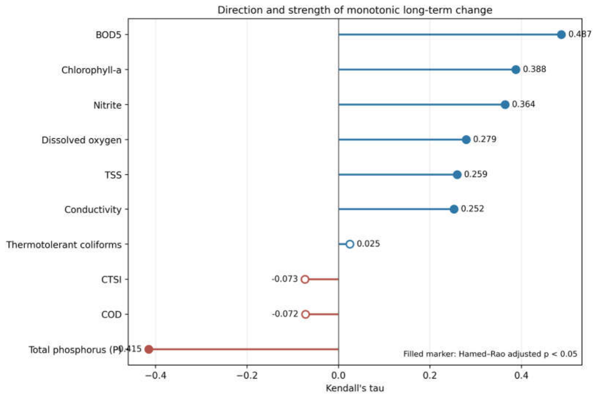
Figure 2. Direction and strength of monotonic long-term change. Filled markers indicate Hamed–Rao adjusted p < 0.05. Annual slopes and block-bootstrap confidence intervals are reported in Table 2.
Preprints 230178 g002
Figure 3. Pettitt change points supported by 12-month block permutation (p < 0.05). Values in parentheses are pre-change and post-change means in the original measurement units. 
Preprints 230178 g003
Figure 4. Spearman correlation matrix. CTSI-component and TN:TP-component correlations are mathematically coupled and should not be interpreted as independent causal effects. 
Preprints 230178 g004
Figure 5. Out-of-time R² for one-month-ahead forecasts. Negative values indicate performance worse than predicting the mean of the evaluation observations. Complete metrics are provided in Table S4.
Preprints 230178 g005
Table 1. Descriptive statistics for monthly water-quality observations, January 2011–September 2025 (n = 177).
Variable Mean SD Median Minimum Maximum
Temperature (°C) 16.60 2.54 17.40 11.10 20.90
Conductivity (µS cm−1) 1706.59 140.51 1704.97 1300.68 2001.60
TSS (mg L−1) 17.53 11.94 13.56 2.00 54.25
Secchi depth (m) 1.31 0.49 1.15 0.45 2.80
Dissolved oxygen (mg L−1) 9.67 2.21 9.51 4.34 16.34
pH 9.30 0.57 9.36 7.56 10.47
Chlorophyll-a (mg m−3) 41.20 28.89 32.55 2.05 128.31
COD (mg L−1) 29.31 8.17 28.80 7.00 45.90
BOD5 (mg L−1) 9.11 4.81 8.06 2.70 32.29
Nitrite (mg L−1) 0.20 0.20 0.15 0.01 1.13
Nitrate (mg L−1) 0.39 0.44 0.26 0.01 3.10
Phosphate, PO4 (mg L−1) 1.38 0.50 1.26 0.17 2.86
Total nitrogen, N (mg L−1) 2.67 1.44 2.42 0.56 9.00
Total phosphorus, P (mg L−1) 1.03 0.78 0.73 0.11 3.50
Ammonium/ammonia (mg L−1) 0.61 0.41 0.59 0.14 2.36
Total coliforms (MPN 100 mL−1) 556.55 531.71 355.00 1.80 1700.00
Thermotolerant coliforms (MPN 100 mL−1) 63.51 88.33 33.00 0.90 445.00
Table 2. Autocorrelation-aware trend results. Confidence intervals use a 12-month moving-block bootstrap; p values are from the Hamed–Rao modified Mann–Kendall test, with trend-free prewhitening (TFPW) as sensitivity analysis.
Variable τ Sen slope 95% block CI p (HR) p (TFPW) ACF1
Conductivity 0.252 13.130 µS cm−1 yr−1 3.368 to 23.158 <0.001 <0.001 0.87
TSS 0.259 0.752 mg L−1 yr−1 0.311 to 1.220 <0.001 <0.001 0.44
Dissolved oxygen 0.279 0.218 mg L−1 yr−1 0.106 to 0.332 <0.001 <0.001 0.49
Chlorophyll-a 0.388 3.254 mg m−3 yr−1 2.136 to 4.363 <0.001 <0.001 0.43
BOD5 0.487 0.547 mg L−1 yr−1 0.353 to 0.744 <0.001 <0.001 0.73
Nitrite 0.364 0.012 mg L−1 yr−1 0.007 to 0.016 <0.001 <0.001 0.40
Total phosphorus (P) -0.415 -0.085 mg P L−1 yr−1 -0.133 to -0.040 0.006 <0.001 0.82
CTSI -0.073 -0.110 units yr−1 -0.316 to 0.078 0.227 0.127 0.45
COD -0.072 -0.046 mg L−1 yr−1 -0.119 to 0.029 0.353 0.123 0.21
Thermotolerant coliforms 0.025 0.000 MPN 100 mL−1 yr−1 -1.201 to 1.063 0.715 0.919 0.19
Table 3. Pettitt change points and mean levels before and after each estimated break. Block p values preserve within-year serial structure; values ≥0.05 are exploratory. 
Variable Change point Mean before Mean after Conventional p Block p
Secchi depth 2013-07 1.66 1.23 0.013 0.321
Total phosphorus (P) 2014-12 2.03 0.66 <0.001 0.005
Dissolved oxygen 2015-07 8.29 10.29 <0.001 0.025
Phosphate (PO4) 2015-11 1.20 1.48 0.006 0.146
TSS 2016-08 10.99 21.60 <0.001 0.002
pH 2016-10 9.06 9.46 <0.001 0.244
Chlorophyll-a 2016-11 21.81 54.18 <0.001 0.002
Nitrite 2017-06 0.11 0.27 <0.001 0.002
BOD5 2018-06 6.54 11.77 <0.001 0.002
Total coliforms 2019-01 439.98 697.89 0.001 0.143
Conductivity 2021-08 1671.60 1798.00 <0.001 0.248
The TP decrease from 2.03 to 0.66 mg P L−1 was not accompanied by lower chlorophyll-a or improved transparency. The decoupling may reflect rapid biological uptake, internal phosphorus recycling, changing hydrology, or a change in monitoring or laboratory practice. Secchi depth, phosphate, pH, total coliforms, and conductivity had small conventional Pettitt probabilities but were not supported by block permutation; these dates should therefore be treated as hypotheses rather than confirmed breaks. 
Table 4. Best leakage-free expanding-window classifier for each contemporaneous task. Positive classes were hypereutrophic state, BOD5 >10 mg L−1 and TTC ≥200 MPN 100 mL−1. Values in parentheses are six-month block-bootstrap 95% confidence intervals.
Task Model Prev. Bal. acc. (95% CI) MCC (95% CI) Sens. Spec. PPV PR-AUC ROC-AUC
Trophic state Random Forest 0.817 0.575 (0.500–0.641) 0.257 (-0.001–0.453) 0.974 0.176 0.841 0.906 0.741
Organic pollution Random Forest 0.516 0.624 (0.529–0.710) 0.347 (0.174–0.490) 0.271 0.978 0.929 0.752 0.693
Fecal-indicator event Logistic Regression 0.086 0.593 (0.392–0.782) 0.130 (-0.129–0.429) 0.375 0.812 0.158 0.224 0.460
Table 5. Persistence and best learned one-month-ahead forecasts. Parentheses are six-month block-bootstrap 95% confidence intervals. ΔRMSE is model RMSE minus persistence RMSE; negative values favor the learned model.
Target Model RMSE (95% CI) MAE Temporal R² (95% CI) ΔRMSE (95% CI)
BOD5 Persistence 4.193 (3.370–5.043) 3.213 0.390 (-0.356–0.560) 0.000 (0.000–0.000)
BOD5 Elastic Net 4.816 (3.436–5.918) 3.416 0.196 (-0.490–0.395) 0.622 (-0.265–1.358)
CTSI Persistence 4.689 (4.024–5.427) 3.648 -0.502 (-0.814–-0.276) 0.000 (0.000–0.000)
CTSI Extra Trees 3.733 (3.170–4.281) 3.002 0.048 (-0.044–0.126) -0.957 (-1.300–-0.630)
TTC (log1p) Persistence 1.715 (1.467–1.908) 1.360 -0.285 (-0.695–0.032) 0.000 (0.000–0.000)
TTC (log1p) Random Forest 1.526 (1.377–1.675) 1.296 -0.018 (-0.162–0.069) -0.188 (-0.396–0.027)
Disclaimer/Publisher’s Note: The statements, opinions and data contained in all publications are solely those of the individual author(s) and contributor(s) and not of MDPI and/or the editor(s). MDPI and/or the editor(s) disclaim responsibility for any injury to people or property resulting from any ideas, methods, instructions or products referred to in the content.
Copyright: This open access article is published under a Creative Commons CC BY 4.0 license, which permit the free download, distribution, and reuse, provided that the author and preprint are cited in any reuse.