

Submitted:
26 August 2026
Posted:
27 August 2026
You are already at the latest version
Abstract
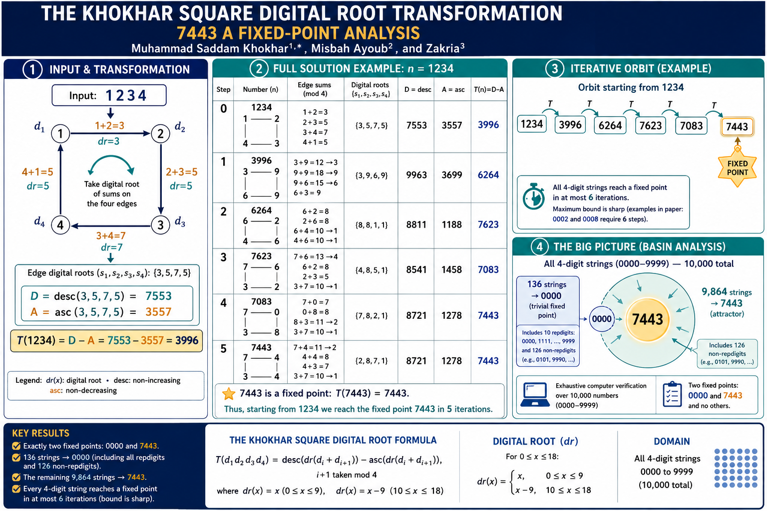
We introduce a deterministic iterative transformation T on four-digit strings. The transforma- tion places the four digits on the vertices of a square, replaces each edge by the digital root of the sum of its two endpoint digits, and subtracts the ascending arrangement of the four re- sulting edge-values from the descending arrangement. We call this the KHOKHAR Square Digital Root Transformation. An exhaustive computer search over all 104 four-digit strings from 0000 to 9999 shows that T has exactly two fixed points, 0000 and 7443, and that every four-digit string reaches one of them within at most six iterations. We give a short, direct proof characterizing exactly which strings map to 0000: a string does so if and only if its four edge digital roots already coincide. This condition holds for exactly 136 of the 10,000 four-digit strings , the ten repdigits together with 126 further, non-repdigit strings such as 0101 and 9990 , which refines the natural first guess that repdigits alone are responsible. The remaining 9,864 strings all converge to the nontrivial fixed point 7443. We close by discussing applications of the construction, and of its exhaustive-verification proof method, in computer science and quantum computing.
Keywords:
digital root
; Kaprekar-type transformation
; fixed point
; functional graph
; exhaustive verification
; Grover’s algorithm
; quantum oracle
MSC: 11A63; 68Q25; 81P68
- In one line: this is a piece of original recreational mathematics in the tradition of Kaprekar’s constant , a small, hand-verifiable digital invariant whose interest lies in its clean proof and its reach into computer-science and quantum-computing pedagogy, rather than in resolving an open problem.
1. Introduction
Iterative maps on the digits of a number often produce unexpected stable constants or cycles; the best-known example is Kaprekar’s routine [1], whose four-digit version famously collapses almost every input to the constant 6174. This paper defines a related but different map, built from a square graph and digital-root arithmetic rather than from sorting the original digits directly. The map is simple enough to compute by hand, yet it has a nontrivial universal fixed point together with a small, exactly characterizable family of exceptional inputs.
The main results, established in the sections that follow, are summarized in the next theorem.
Theorem 1
(KHOKHAR Fixed Point and Convergence Theorem). Let T be the KHOKHAR Square Digital Root Transformation defined in Section 3. Then:
- (a)
- and , and these are theonlytwo fixed points of T.
- (b)
- For every four-digit string n, some iterate with lies in ; the bound 6 is sharp.
- (c)
- if and only if the four edge digital roots of n (Section 3) are all equal to one another. Exactly 136 of the four-digit strings satisfy this condition. The other strings, including 7443 itself, satisfy for some k with .
Part (a) is the headline fixed-point result. Part (c) is the more delicate of the three claims: it would be natural to guess that repdigits alone feed into 0000, but the true condition is a fact about the four edge values , of which the repdigit case is only a special (if the most visually obvious) instance. Part (b) gives a concrete worst-case iteration bound.
2. Definitions and Notation
Let be a four-digit string with digits . Leading zeros are allowed and are always retained.
2.1. Digital Root
For a nonnegative integer x, the digital root is defined by
where is the sum of the decimal digits of x. In this paper x is always the sum of two digits, so , and the digital root reduces to the simple closed form
2.2. Descending and Ascending Arrangements
If are four single-digit numbers, then is the four-digit string obtained by writing in non-increasing order, and is the four-digit string obtained by writing them in non-decreasing order. Leading zeros are kept. For example,
3. The KHOKHAR Square Digital Root Transformation
We place the digits on the four vertices of a square, in cyclic order (Figure 1). The four edges of the square are
On each edge we compute the digital root of the sum of its two endpoint digits:
We then form two four-digit strings from the multiset :
and define the transformation by
written as a four-digit string, with a leading zero if necessary. Because D and A arrange the same multiset of four digits, always, so is a well-defined value between 0000 and 9999 (Lemma 1 below makes precise exactly when ).
Equivalently, this is the KHOKHAR Square Digital Root Formula:
4. Worked Example
We illustrate T starting from . Every step below was independently verified by hand and by computer.
Step 1: 1234
Edge sums: . Digital roots: .
Step 2: 3996
Edge sums: . Digital roots: .
Step 3: 6264
Edge sums: . Digital roots: .
Step 4: 7623
Edge sums: . Digital roots: .
Step 5: 7083
Edge sums: . Digital roots: .
Step 6: 7443 (fixed-point check)
Edge sums: . Digital roots: .
Hence 7443 is a fixed point of T, and 1234 reaches it after exactly five iterations.
5. Multiple Starting Points Converging to 7443
6. The Basin of Zero: Repdigits and Their Exact Characterization
6.1. The Repdigit Case
If all four digits are equal, say , every edge sum equals , so all four edge digital roots automatically coincide: . For example, take : every edge sum is , with digital root 1, so all four edge values equal 1. Then , and
The same argument applies verbatim to every repdigit, so all ten strings map directly to 0000.
6.2. An Exact Characterization
The repdigit computation above suggests, at first glance, that precisely when n itself is a repdigit. This natural guess conflates a sufficient condition on the original digits with the true necessary-and-sufficient condition, which lives one level down, on the edge values .
Lemma 1.
For single-digit values ,
Proof.
Sort the multiset as ; then and termwise. These two 4-tuples agree exactly when and ; but together with forces all four to be equal. The converse is immediate. □
Corollary 1.
if and only if the four edge digital roots of n are all equal to one another; and whenever this happens, n reaches 0000 in a single step.
Repdigits satisfy the hypothesis of Corollary 1 for the reason given in Section 6.1: all four raw edge sums coincide (not merely their digital roots), because every edge joins two copies of the same digit. But Corollary 1 only requires the digital roots to coincide, and a digital root discards information , two different sums can share a root whenever they differ by 9. This opens the door to non-repdigit strings whose edge sums differ but whose digital roots happen to agree. For instance, has edge sums , not all equal , but their digital roots are , all equal, so directly, even though 0191 is not a repdigit.
6.3. Enumerating the Full Basin
Exhaustive search (Section 8) over all four-digit strings finds exactly 136 strings satisfying the condition of Corollary 1 , not the 10 repdigits alone:
- 10 repdigits, where all four raw edge sums already coincide by symmetry;
- 90 further strings where the four raw edge sums still coincide exactly (typically alternating patterns such as ), bringing the total of this “trivial” type to 100;
- 36 additional strings where the raw edge sums do not all coincide, but their digital roots do, as in the 0191 example above.
Table 3 lists a representative sample spanning the full range; the complete list of 136 strings was produced by the program in Section 8.
Consequently, exactly four-digit strings converge to 7443; the 126 non-repdigit exceptions above join the 10 repdigits in the basin of 0000 instead.
7. A Sharp Convergence Bound
Beyond identifying the two fixed points, it is natural to ask how quickly an arbitrary input converges.
Theorem 2
(Sharp Convergence Bound). For every four-digit string n, for some , and this bound is sharp: it is achieved by of the strings, including (Table 2).
Table 4 gives the complete distribution, obtained by iterating T from every one of the starting strings and recording the number of steps needed to first land on 0000 or 7443.
8. Proof by Exhaustive Computation
Theorem 1 and Theorem 2 are established by direct computation: T is applied to every one of the possible four-digit strings, and every resulting orbit is traced until it reaches a fixed point. Because the entire domain has only elements, this is a complete case analysis, not a sample , there is no input left unchecked. The verification program below applies T to every four-digit string, records which of the two fixed points each orbit reaches, and counts how many steps that takes.
| Listing 1: Verification script. |
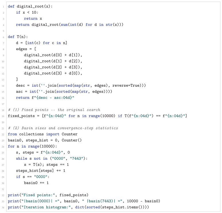 |
Running this program produces:
 |
which confirms every numerical claim in Theorem 1 and Theorem 2: exactly two fixed points, a basin of size 136 for 0000 and for 7443, and a maximum convergence time of six iterations. No starting value failed to reach a fixed point within this bound, and no cycle of length greater than one was found anywhere in the state space, so these two fixed points are the only eventual behavior T can exhibit.
9. Applications in Computer Science
The construction above is primarily a recreational and pedagogical one, in the tradition of Kaprekar’s routine. Even so, both the transformation itself and the exhaustive-verification method used to analyze it connect naturally to several standard topics in computer science.
9.1. Finite Functional Graphs and Cycle Detection
Because T maps a finite state space of size to itself, repeatedly applying it to any starting point traces a path that must eventually enter a cycle , here, one of the two fixed points. The resulting structure (a collection of trees hanging off two single-node cycles) is exactly the “functional graph” or “rho shape” that underlies cycle-detection algorithms such as Floyd’s [2] and Brent’s [3] algorithms, which are used in practice for testing pseudorandom number generators, in Pollard’s rho method for integer factorization, and in detecting cycles in pointer-based data structures. Because the KHOKHAR transformation’s state space is small enough to enumerate completely (Section 8), it makes a convenient hand-sized instance on which to first implement and test a cycle-detection algorithm before applying it to state spaces too large to enumerate exhaustively.
9.2. Termination Proofs and Worst-Case Iteration Bounds
Theorem 2 is, in miniature, exactly the kind of claim a computer scientist must establish to certify that an iterative procedure terminates and to bound its running time: not just “it always stops,” but a concrete worst-case count, together with a witness showing the bound cannot be improved. The proof technique here , exhaustively simulating every possible input and recording the observed iteration counts , mirrors how worst-case bounds are frequently first discovered empirically before a general argument is sought. Kaprekar’s routine [1], whose analogous four-digit bound is seven iterations, is used pedagogically in much the same way; the KHOKHAR transformation offers a second, independent example with a different graph-theoretic flavor.
9.3. Exhaustive Search as a Verification Technique
The proof in Section 8 is a working example of exhaustive model checking: a universally quantified claim (“for all four-digit strings n, ...”) is verified not by a general argument but by checking every one of the finitely many cases on a computer. This is the same idea underlying model checkers used to verify finite-state hardware and protocol designs, and it is feasible here only because the state space () is small enough to enumerate in well under a second. The construction is therefore a natural teaching example for discussing the boundary between problems small enough for brute-force verification and problems large enough (e.g. a state space of ) to require symbolic techniques, SAT/SMT solvers, or randomized/property-based testing tools, which sample rather than exhaust the input space.
9.4. A Self-Contained Programming Exercise
Implementing T requires only digit extraction, small modular (digital-root) arithmetic, sorting, and careful string formatting to preserve leading zeros , a compact but realistic set of tasks for an introductory programming exercise. Because the correct answer for any input is unambiguous and easy to check by hand (Section 4), the transformation is well suited to test-driven or unit-testing exercises, for example asserting that T("1234") == "3996", or that every orbit reaches a fixed point within six steps as predicted by Theorem 2.
9.5. A Cautionary Example for Hash and Checksum Design
On first inspection, T resembles the kind of ad hoc digit-mixing step sometimes proposed for a simple checksum or hash function: it combines all four input digits nonlinearly and appears to scramble them. The analysis above shows the opposite of good hashing behavior, however: iterating T collapses nearly every input onto just one of two possible outputs, and Corollary 1 shows that even a single application is far from uniform, since 136 distinct inputs are all mapped to the same output 0000. This makes the KHOKHAR transformation a useful negative example when teaching hash-function design: a function that “looks scrambled” by inspection can still have catastrophic collision behavior, which must be checked explicitly (as Section 8 does here) rather than assumed. T is offered purely as a recreational and pedagogical construction and should not be used as an actual checksum, hash function, or pseudorandom generator.
9.6. A Small Dataset for Visualization Practice
The basin sizes and iteration-count distribution computed in Section 6, Section 7 and Section 8 constitute a complete, self-generated dataset of labeled points, together with a discrete distribution over seven iteration-count values (Table 4). This provides ready material for practicing basic data-visualization tasks , for example, a bar chart of the two basin sizes, or a histogram of convergence lengths , without needing to source any external data.
10. Applications in Quantum Computing
The verification task of Section 8 , decide, for every one of four-digit strings, whether a given predicate holds , is a textbook instance of unstructured search, the problem class for which quantum computers offer a proven speedup. This section spells out how quantum search and counting algorithms apply to the KHOKHAR transformation, and is equally explicit about the limits of that connection at this problem size.
10.1. Grover-Accelerated Search Over the State Space
Classically, deciding whether a marked element exists among N unordered candidates requires oracle evaluations in the worst case , exactly what Section 8 does, evaluating T on all strings. Grover’s algorithm [4] finds a marked element among N candidates using only oracle queries. Because exactly, this is an unusually clean instance to state: a Grover search for, say, a counterexample to the six-iteration bound of Theorem 2, or for a member of the 136-element zero-basin of Corollary 1, would need on the order of 100 oracle calls in place of classical evaluations of T , a hundredfold reduction in queries, exactly matching the quadratic speedup Grover’s algorithm guarantees.
A caveat is essential here. Grover’s algorithm returns a marked element with high probability; it does not, by itself, certify that no marked element exists the way the classical exhaustive proof of Section 8 does. Matching the deductive certainty of brute-force enumeration requires either running Grover search to (probabilistic) exhaustion or using the quantum counting technique of Section 10.4, which bounds the exact number of solutions.
10.2. Reversible Oracle Construction
Quantum query algorithms act on a unitary oracle, but T itself is not reversible: Corollary 1 shows 136 distinct inputs collapse to the single output 0000, so T cannot be implemented directly as a quantum gate. The standard remedy [6] is to embed the classical function in a larger reversible map via an ancilla register,
or, for a single-bit predicate such as “does n satisfy Corollary 1?”, a phase oracle . Building requires reversible circuits for each stage of the transformation: digit extraction, digital-root reduction of a sum in , a four-element sorting network for desc and asc, and a final subtraction. Reversible adders such as the Cuccaro ripple-carry adder [7], together with reversible comparators of the same style, are exactly the primitives needed to assemble such a circuit. This makes the KHOKHAR transformation a compact, fully worked example for practicing the classical-function-to-reversible-oracle compilation step that underlies essentially every quantum query algorithm, including Grover’s.
10.3. Qubit Budget for a State-Space Index
Encoding a single four-digit string in binary-coded decimal costs qubits (four bits per digit); indexing the valid strings directly costs only qubits. Either count is modest , comparable to circuit widths already exercised on current superconducting and trapped-ion hardware , though the arithmetic subcircuits of Section 10.2 would add nontrivial depth beyond the bare index register. The state space of the KHOKHAR transformation is therefore a plausible size for a circuit-design exercise (building and running Grover’s algorithm on a simulator or small device), even though, as Section 10.5 makes clear, it is far too small to need a quantum computer in practice.
10.4. Quantum Counting to Certify the Basin Sizes
Grover’s algorithm alone answers “does a marked element exist?”; quantum counting [5], which combines amplitude amplification with quantum phase estimation, estimates how many marked elements exist using the same query budget, and with enough precision can pin the count down exactly. Applied here, quantum counting offers a route to certifying the two basin sizes established by brute force in Section 8 , and , using asymptotically fewer oracle evaluations than the classical count. This illustrates that it is not only the “find one” step of a verification proof that admits a quantum speedup, but the “count them all” step as well.
10.5. A Note on Scale
None of the above should be read as a claim that a quantum computer is useful here: at , the classical exhaustive check of Section 8 already completes in a small fraction of a second, and oracle calls carries no practical advantage over classical ones at this scale, especially once the overhead of building is included. The value of the connection is pedagogical: the KHOKHAR transformation’s state space is small enough to reason about completely by hand or by brute force (Section 6, Section 7 and Section 8), yet structured simply enough to serve as a concrete worked example when teaching Grover’s algorithm, reversible oracle construction, and quantum counting , the same role Kaprekar’s routine and other small combinatorial puzzles have long played for classical-algorithms pedagogy.
11. Conclusion
We have introduced and exhaustively verified a new iterative map, the KHOKHAR Square Digital Root Transformation, defined by digital-root addition along the edges of a square together with a descending-minus-ascending digit-sort step. The map has exactly two fixed points, 0000 and 7443, and every four-digit string reaches one of them within at most six iterations. We gave a short direct proof (Lemma 1 and Corollary 1) characterizing exactly which strings reach 0000: those whose four edge digital roots already coincide. This condition holds for 136 strings , the 10 repdigits together with 126 further, non-repdigit strings. The remaining strings all converge to the single nontrivial constant 7443.
| The KHOKHAR transformation has a unique nontrivial fixed point, 7443, reached (within six steps) by all but 136 of the four-digit strings. |
Beyond its interest as a hand-computable digital constant in the tradition of Kaprekar’s routine, both the transformation and its exhaustive-verification proof serve as compact case studies relevant to functional-graph analysis, termination proofs, brute-force program verification, and hash-function pedagogy (Section 9), as well as to Grover-type quantum search and quantum counting (Section 10).
Supplementary Materials
The following supporting information can be downloaded at the website of this paper posted on Preprints.org.
Acknowledgments
The authors thank their colleagues at the College of Information and Artificial Intelligence, Yangzhou University, and the Department of Computer Science, Sukkur IBA University, for their valuable discussions and support. The authors also acknowledge the use of open-source tools and libraries that facilitated this research.
Data Availability Statement
All data generated or analyzed during this study are included in this published article and its supplementary information files. The source code are publicly available via the GitHub repository: https://github.com/saddam232003/KHOKHAR-Square-Digital-Root-Transformation. To reproduce the results, clone the repository and run the GUI:
-
git clone https://github.com/saddam232003/KHOKHAR-Square-Digital-Root-Transformation.gitcd KHOKHAR-Square-Digital-Root-Transformationpython "Khokhar Digital.py"
Conflicts of Interest
The authors declare no conflicts of interest.|
The construction, the theorems, and their proofs in Section 1, Section 2, Section 3, Section 4, Section 5, Section 6, Section 7 and Section 8 are original to this work and require no external references; to the best of the author’s knowledge, this specific square-graph digital-root transformation has not previously appeared in the literature. The references below support the comparisons and applications drawn in Section 9 and Section 10.
References
- Kaprekar, D. R. An Interesting Property of the Number 6174. Scr. Math. 1955, 21, 304. [Google Scholar]
- Knuth, D. E. The Art of Computer Programming, Volume 2: Seminumerical Algorithms, 3rd ed.; Addison-Wesley: Reading, MA, 1998. [Google Scholar]
- Brent, R. P. An improved Monte Carlo factorization algorithm. BIT 1980, 20(2), 176–184. [Google Scholar] [CrossRef]
- Grover, L. K. A fast quantum mechanical algorithm for database search. In Proceedings of the 28th Annual ACM Symposium on Theory of Computing (STOC ’96); 1996, ACM; pp. 212–219.
- Brassard, G.; Høyer, P.; Tapp, A. Quantum counting. In Proceedings of the 25th International Colloquium on Automata, Languages and Programming (ICALP ’98); Lecture Notes in Computer Science vol. 1443; Springer, 1998; pp. 820–831. [Google Scholar]
- Nielsen, M. A.; Chuang, I. L. Quantum Computation and Quantum Information. (first published 2000), 10th Anniversary ed.; Cambridge University Press: Cambridge, 2010. [Google Scholar]
- Cuccaro, S. A.; Draper, T. G.; Kutin, S. A.; Moulton, D. P. A new quantum ripple-carry addition circuit. arXiv 2004, arXiv:quant-ph/0410184. [Google Scholar]
Figure 1.
The four digits of placed on a square in cyclic order. Each edge is the digital root of the sum of its two endpoint digits.
Figure 1.
The four digits of placed on a square in cyclic order. Each edge is the digital root of the sum of its two endpoint digits.
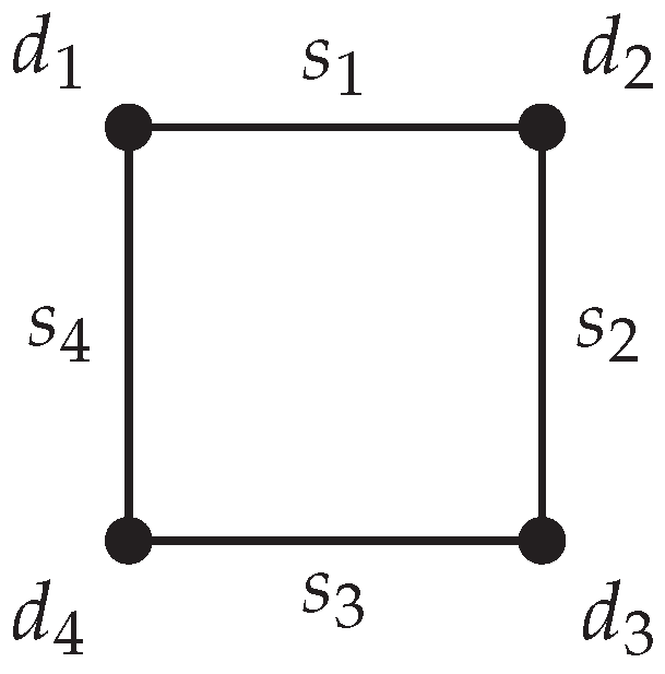

Table 1.
Sample orbits converging to the nontrivial fixed point 7443.
| Starting number | Orbit |
|---|---|
| 0001 | |
| 1112 | |
| 2468 | |
| 1357 | |
| 9998 | |
| 1234 |
Table 2.
The longest possible orbits: two witnesses achieving the maximal six-iteration bound of Theorem 2.
Table 2.
The longest possible orbits: two witnesses achieving the maximal six-iteration bound of Theorem 2.
| Starting number | Orbit |
|---|---|
| 0002 | |
| 0008 |
Table 3.
A representative sample of the 126 non-repdigit strings lying in the basin of 0000.
| Representative non-repdigit members of | |||||
|---|---|---|---|---|---|
| 0101 | 0191 | 0202 | 0909 | 1010 | 1019 |
| 1910 | 1919 | 2020 | 2029 | 2920 | 2929 |
| 5050 | 5059 | 5950 | 5959 | 8080 | 8989 |
| 9090 | 9099 | 9101 | 9191 | 9909 | 9990 |
Table 4.
Distribution of the number of iterations k required for to first land on a fixed point, over all four-digit strings n.
Table 4.
Distribution of the number of iterations k required for to first land on a fixed point, over all four-digit strings n.
| Iterations k | Number of strings |
|---|---|
| 0 | 2 |
| 1 | 350 |
| 2 | 1536 |
| 3 | 1528 |
| 4 | 3688 |
| 5 | 1800 |
| 6 | 1096 |
| Total | 10,000 |
Disclaimer/Publisher’s Note: The statements, opinions and data contained in all publications are solely those of the individual author(s) and contributor(s) and not of MDPI and/or the editor(s). MDPI and/or the editor(s) disclaim responsibility for any injury to people or property resulting from any ideas, methods, instructions or products referred to in the content. |
© 2026 by the authors. Licensee MDPI, Basel, Switzerland. This article is an open access article distributed under the terms and conditions of the Creative Commons Attribution (CC BY) license (http://creativecommons.org/licenses/by/4.0/).
Copyright: This open access article is published under a Creative Commons CC BY 4.0 license, which permit the free download, distribution, and reuse, provided that the author and preprint are cited in any reuse.