

Submitted:
26 August 2026
Posted:
27 August 2026
You are already at the latest version
Abstract
This paper is a literature study supplemented with self-collected data on fish density, age and growth of smelt (Osmerus eperlanus) in Lake Mjøsa over the last 40 – 50 years. Smelt is an important prey fish for piscivorus brown trout, and the development of the brown trout population is illuminated by catch reports. The smelt abundance in Lake Mjøsa declined in the period 1980 to 1990 but increased sharply in 2018 and 2023. Re-cruitment to the smelt population is positively correlated with air temperature in May and July. Increased smelt abundance is a possible reason why the population of large grown brown trout also appears to have increased, while smelt has shown reduced in-dividual growth in recent years. The brown trout population does not appear to have a decisive effect on the smelt stock but may have contributed to increased mortality in smelt in the material from 2006 - 2022 as compared to 1980. The effect of brown trout stocking, conducted for the last time in 2021, is uncertain, but future catch reporting will provide a better answer to this.
Keywords:
population growth
; biomass
; production
; year-class strength
; temperature
; time trends
1. Introduction
Smelt (Osmerus eperlanus) (Figure 1) is a bony fish in the family Osmeridae, order Osmeriformes. The species’ natural distribution in Norway is limited to areas below the upper marine limit in river systems from the Swedish border in the east to Agder County, southernmost Norway in the west. It lives in freshwater and brackish water [1] and can be anadromous [2]. Smelt populations are dominated by individuals less than 15 cm and are an important prey fish for piscivorous brown trout (Salmo trutta) and perch (Perca fluviatilis). Smelt is versatile in its choice of food from juvenile to adult. It can eat algae, though zooplankton is most important [3,4]. It is also piscivore and eats its own fry [4,5,6]. It has been released (now illegal) into several waters to promote large grown brown trout [7,8,9]. In some populations, such as in Lake Mjøsa, the smelt shows two different life history strategies. In addition to the “normal” smelt, there is a more piscivorous large morph (up to 30cm) [5,8].
Smelt is an important zooplankton predator in competition with vendace (Coregonus albula) and whitefish (Coregonus lavaretus) [3] and can affect the occurrence of algae-eating zooplankton in groups such as Daphnia spp. and Bosmina spp. [10]. Plankton-eating fish species are ecologically important as predators in open water, and they are correspondingly important in a monitoring context. The pelagic fish populations in Mjøsa are now monitored with annual echo sounder recordings, as one of several fortunate outcomes of the EU Water Frame Directive (WFD).
The growth of animal populations is determined by recruitment and mortality, and recruitment of fish populations is affected by environmental conditions that may vary from year to year and can be seen in fluctuating year-class strength. Year-class strength has been found to be positively correlated with summer temperatures in several lake-spawning fish species [11,12,13,14,15,16]. Year-class strength of smelt in the Swedish lakes Väneren and Vettern, is positively correlated with air temperature in April [17]. In populations of the closely related rainbow smelt (Osmerus mordax) in Lake Erie and Lake Ontario in North America, year-class strength is negatively correlated with the abundance of one-year old conspecifics feeding on larvae and fry [18,19]. Keller and Molenaar [20] found in a Dutch lake that high temperatures in May, i.e., during the incubation period of the smelt eggs, led to the eggs hatching before there was sufficient planktonic nutrition available for the larvae. This is because the development of plankton is controlled more by light than by temperature, and this “mismatch” caused reproduction to fail in years with high May temperatures.
This article describes development trends in the smelt stock in Lake Mjøsa in part regarding this species role as prey fish for the large growing Mjøsa brown trout. The stock is assumed to constitute a metapopulation consisting of several subpopulations with different spawning grounds with a certain genetic exchange. The study is based on previously reported studies, and on newer material collected at the smelt spawning grounds in Furnesfjorden, a part of Lake Mjøsa. Assessments of the development of the brown trout population are made based on catch reports from fishery. Recruitment and year-class strength of smelt are analysed in relation to air temperatures in the spring and summer months, in relation to year-class strength of 1+ (expressing predation risk) and 3+ (expressing population fecundity) smelt, and in relation to water level development in Mjøsa, which normally increases through the latter half of May and in early June when smelt spawning and hatching occur. Water temperature is believed to be most important for the development of aquatic ectothermic animals, and it is positively correlated to air temperature [16], which is used here as a predictor in linear models for relative year-class strength as there exist long measurement series from several measuring stations, including at Kise by Furnesfjorden.
2. Materials and Methods
2.1. Study Area
Mjøsa (Figure 2) is the largest lake in Norway with a surface area of 365 km2. The lake has been regulated since 1858 and has since 1961 been regulated 3.6 m (119.3 - 122.9 m a.s.l.) with a dam in Svanfossen 22 km down the outlet-river Vorma (60° 23’ 50” N, 11° 14’ 11” E). The greatest measured depth is 453 m. The water quality in Mjøsa has varied over the last 60 - 70 years. In the 1970s, there were relatively high concentrations of plant nutrients, phosphorus and nitrogen, and there were problems with algae and blue-green bacteria growth. Phosphorus was given the greatest attention since it is normally the minimum factor for production in freshwater [21]. The concentration of total phosphorus (TP) was often higher than 9 μg/l, which is the upper limit for the class “Good water quality” in the WFD [22]. Concentrations from 9 - 16 μg/l are classified as “Moderate”, a condition that should trigger improvement measures. Phosphorus purification of wastewater and widespread controls and measures in the lake’s catchment area as part of the “Mjøsa Action” have resulted in significant improvements [23]. However, phosphorus levels have shown a worrying increase after periods of rain and flooding, and in recent decades there have been blooms of algae and blue-green bacteria in summers of long periods of sunshine [24].
There are 20 naturally occurring fish species in Mjøsa [25] and smelt, vendace and whitefish have dominated the pelagic zone [26,27]. Two Percids, perch and ruffe (Gymnocephalus cernua), six cyprinids (Cyprinoformes) and pike (Esox lucius) dominate the littoral and benthic zone, in addition to the bottom-dwelling cod fish, the burbot (Lota lota). The vendace fishery in Mjøsa and the tributary Lågen has been of economic importance [28] but has declined sharply in the last 20-30 years [29,30], partly due to reduced stocks. For anglers, the large grown brown trout is a favourite, but perch and pike are also targeted. Gillnet catches per effort of brown trout seem to have increased in the last 20 - 30 years, whereas trolling and angling catches per effort fluctuate [31,32].
Findings of organic toxins in brown trout [33] put an end to commercial exploitation of brown trout for a period, and gillnet fishing declined. In the years 1973 - 1990, an average of approximately 17,000 artificially bred two-year old brown trout of the Hunder falls population were released annually by the power company Glommen and Laagen Brukseierforening, later Hafslund. The number increased to an average of 23,000 fish annually from 1991 by producing and releasing fish from several local strains (such as the rivers Brumunda and Lena). This, in combination with catch-and-release practices among anglers, may have contributed to an increased trout population. Most brown trout are although naturally recruited from tributary rivers of which the main inlet River Lågen/Hunder falls is clearly the largest [34]. Brown trout from the size of 20-25 cm starts to eat smelt, and this doubles their annual length increment [35,36,37]. They gradually switch to larger prey such as vendace and whitefish [38].
Smelt is caught with dipnets from boats or along the shore, previously also with push seines during its spawning season to be used as bait for trout and perch fishing. This fishery is unlikely to have any impact on smelt abundance.
2.2. Methods
Density and biomass of smelt estimated by means of echosounding are taken from Lindem and Sandlund [39], Sandlund, Næsje [27], Gjelland, Eikland [40] and Eikland, Gjelland [41], and from two own recordings with a single beam SIMRAD EK15 echosounder [42] (with 9ᵒ beam angle) in Furnesfjorden on 20 May 2021 and 15 May 2024. SIMRAD EK15 has been shown to give well comparable results with the older type SIMRAD EY M [43], which was used in the surveys in 1980 and 1990 -1991 Sandlund et al. 1992. The use of SIMRAD EK15 is described in more in details by Linløkken, Næstad [43] and Linløkken [44]. Echo strength (TS, dB) is transformed to fish length (L, cm) by the formula: TS (dB) = 20 • log (L, cm) - 68 [39], and further to weight/biomass (W, g) by known or assumed ratio between fish length and weight: W = a • Lb, where a and b are parameters in the regression: log W = b • log L+ log a. This ratio varies between species, populations and sex (mature), and can, when species composition is known, be used to calculate weight/biomass of species. Mean weights for each species from trawl catches can also be used. It is regrettable that not all echo sounder surveys are reported with density (N/ha) distributed by species. Often only biomass is presented by species, calculated by different methods, all of which introduce new variance in the estimate, and makes it difficult to compare studies.
Smelt were collected with dipnets in May 2006, 2007, 2008, 2014, 2015, 2016, 2018, 2019 and 2022 along the shores at spawning grounds between Hamar and Brumunddal on the east side of Furnesfjorden, a part of Lake Mjøsa (Figure 2). Spawning takes place during the darkest time of day, according to Sandlund, Klyve [5], most intensely around 02:00 (CET, not summertime). When sampling at the spawning ground with a dipnet, the catchability of large grown smelt is low and the inclusion of these is not representative. In 2018 and 2022, extra effort was made to catch large smelt by selectively going after them with the dip net. In May 2008, Nordic sample nets (12 mesh sizes from 5 - 46 mm) were used [45]. In previous studies, seines and nets were also used for collection [5,25].
The length of smelt was measured (L, mm), from the tip of the snout to the end of the tail fin when it is naturally extended (natural length), and weighed (W, 0.1 g). Age was determined by analysis of saccule otoliths that were read twice under a stereo microscope (10 x 40 magnification) before being burned, cracked and read again in cross-section. Experience has shown that it can be easy to overlook zones from the third and especially from the fourth winter zone and older otoliths (i.e. in sexually mature fish) in unburned otoliths. Age and growth from earlier periods are taken from [25] and [5] and compared with analyses of material from 2006-2022. Growth is presented as mean lengths Lt (empirical growth) and as instantaneous growth rates (Gt) at age t: Gt = ln (Wt+1/Wt) where Wt is weight at age t, calculated from length Lt and the relationship Wt = a • Ltb. Fish lengths from the 2006 – 2022 material were tested for variation between years with a linear model [46] with ln (Age) as continuous, and growth year (catch year – 1) as categorical predictor.
Annual survival (S), mortality A = 1 – S and instantaneous mortality Z = - ln S (S = e-Z) are based on catch curves and calculated using a method described by Chapman and Robson [47] and Robson and Chapman [48]. When catch curves (age distribution in the catch) are used, it is important that all age groups included have approximately the same catchability. This is often not the case for the youngest age group because small fish are less catchable, especially with gill nets. Smelt caught on the spawning grounds are assumed, with few exceptions, to be sexually mature, i.e. males and females aged 2+ and older, in some years only 3+ and older [8]. The age group 2+ may be underrepresented because not all are sexually mature, while 1+ smelt were not caught on the spawning grounds.
Chapman and Robson [47] provide a chi-square test to check whether the youngest age group is fully recruited. In material with few fully recruited age groups and varying year-class strength, the method will be inapplicable.
Year-class strength is calculated by the ratio between observed number of fish (NO,t) of age group t in a sample and the expected number of fish (NE,t) of the same age group. Constant recruitment and mortality are assumed, and the expected number is calculated by: NE,t = S • Nt-1 for each age group. The ratio NO,t/NE,t giving an expression for relative strength for age group t [16]. A linear model was used to test the relationship between relative year-class strength and four continuous predictors: 1.) mean air temperature (in the months of April, May, June, July and August) (temp), 2.) Water level change in Lake Mjøsa from 15 May to 7 June in the years 1969 to 2020 (∆h, m), 3.) year-class strength of 1+ smelt (ln (YCS.1+), predation risk) (ln to normalize data) and 4.) year-class strength of 3+ smelt (ln (YCS.3+, population fecundity), as most of a cohort normally is mature at this age.
YCS = b0 + b1• temp + b2 (∆h) + b3 • ln (YCS.1+) + b4 • ln (YCS.3+)
∆h averaged 1.14 m and varied from -0.63 to 3.14 m in the years 1969 to 2020.
2.3. Population Dynamics and Production
As an alternative method to calculate population mean weight (WM) and biomass (B) and, to calculate production (P), life history tables [49,50] were constructed by calculating the number of fish (Nt) in age groups t ≥ 1+, as follows: Nt = S • Nt-1. Biomass (Bt) is given by the number of fish (Nt) in age group t multiplied by the mean weight Wt in the age group: Bt = Nt • Wt. Mortality is assumed to be constant throughout the year (a simplification), while growth is limited to an assumed period of four months, from the first of June to the first of October. The table is divided into periods; with and without growth. Annual Z is (as logarithm) additive and gives, divided by 12, instantaneous mortality per month. Instantaneous mortality during the growth period is 4 • Z/12 = Z/3, and instantaneous mortality during the period without growth is 8 • Z/12 = 2 • Z/3. The material from 2006-2022 was stored in a freezer (-20 ᵒC) before sampling, which can lead to drying and weight loss. The length-weight relationship is therefore compared with older data from material that was sampled in a fresh state, from [5]: W = 0.0032 • L3.160.
Annual production in an age group t is given by the mean biomass (BM) in the growing season multiplied by Gt. Mean density (NM) is calculated as follows: NM = N0 • e-M/2, where N0 is the population at the start of the growing season (May) and M = instantaneous mortality during the growing season (M/2 for half a season). Mean biomass (BM) is calculated as: BM = NM • W0 • eG/2 (W0 = weight before growth season), and the production Pt = BM • Gt for each age group. The values are summed over the age groups and by iteration the number of recruits (N01) (i. e., number of 1-year-olds at the start of the season) can be chosen so that the sum of the mean density (NM) or biomass (BM) corresponds to a chosen quantity, such as fish density or biomass estimated by means of echosounding.
2.4. Brown Trout Assessments
Data for brown trout fishing are taken from Qvenild and Nashoug [51], from catch reports from fishermen who obtained fishing licenses (Brumunddal and Omegn Sportsfiskerforening) for Brumunda in 2007–2009, and from catch reports received by the State Administrator in County Oppland/Innlandet [31,32].
3. Results
3.1. Biomass and Species Composition in the Open Water Bodies
Echo recordings in 1978-1980 and 1990-91 showed a sharp reduction in pelagic biomass, from 25.2 to 4.4 kg/ha during the intervening decade (Figure 3). The reduction was most pronounced for whitefish with 91% and vendace with 88%, as compared to only a 17% reduction for smelt. This was followed by a fivefold increase of smelt from 1990-1991 to 2018. The smelt increase may have been a result of reduced competition from vendace and whitefish.
The smelt abundance declined between 2018 and 2020, but has increased since then, and in 2023, 15.8 kg smelt/ha was estimated, the highest estimate ever for smelt. The stock of vendace has been low since 1990 but increased to nearly 6 kg/ha in 2023, the highest estimate of vendace since 1980. From 2020 to 2023, the whitefish stock increased and was then estimated at just under 28 kg whitefish/ha, the highest estimate ever made for whitefish.
The biomass reduction from 1980 to 1990 was explained by the fact that productivity in Lake Mjøsa decreased after the cleaning measures that were implemented [27]. It is more difficult to explain the large increase occurring after 2018 [41]. The total phosphorus concentration in the upper water layer of Mjøsa varied between 2.5 and 7.8 μg/l in 2023, with an average of 5 μg/l, a condition characterized as Good [52]. Increasing temperatures over several decades may have contributed to increased biomass by increasing recruitment in several fish species. One effect of higher temperatures is a prolonged growing season, commonly resulting in larger fry with higher survival in the first winter [11,13].
Biomass calculations from 1978-1980 and 1990-1991 were based on an assumed mean weight of WM = 10 g for smelt [27]. In the later study, biomass is calculated from echo strength, but it is unclear how the transformation was done. Mean lengths of normal smelt (≥ 1+) in trawl catches from 2023 varied between habitats from 9.0 to 9.7 cm, and Foulton’s condition factor K = 100 • W/L3 ranged from 0.49 to 0.52 [53], and this gives WM = 3.6 - 4.7 g.
On 20 May 2021, registrations in Furnesfjorden showed a mean density of 2666 fish per ha in size approx. 5 – 50 cm (TS = [-54 to -33 dB]) (Table 1). The fish were distributed at 15 - 60 m depth in the pelagic zone (Figure 4), and the fish density was calculated in this cone segment. There were 1599 fish/ha in the length group approx. 5 – 13 cm (TS = [-54 to -46 dB]), which are essentially normal smelt at age ≥ 1+, with elements of one-year-old vendace and whitefish. These appear as a peak between approximately 7 and 13 cm in the length distribution based on echo strength (Figure 5). WM in this length group was calculated to be 3.9 g by transforming echo strength frequency to weight.
The fish density in Furnesfjorden in 2021 was higher than that calculated for the whole of Lake Mjøsa in 1978 – 1980, but it was lower than that calculated for the whole lake in 2023 [41]. This corresponds to the density differences between Furnesfjorden and the whole lake reported in 1990 [27]. The density calculations from Furnesfjorden on 15 May 2024 gave 1110 fish/ha of smelt size. This was a significant density reduction (non-overlapping C.I.) of 30% as compared to May 2021.
3.2. Length Distribution in the Dip Net Catches
The length distributions (Figure 6) of smelt varied widely between years, but were dominated by three to six cm groups, from 8 to 14 cm. The mean length of sexually mature smelt in the dipnet catches from 2006-2022 varied from 9.8 to 12.0 cm, and the average weight varied from WM = 2.9 to 7.3 g. The length-weight ratio from Sandlund et al. [15]) gives WM = 4.3 and 8.3 g for the same fish lengths (still lower than 10 g even though this only includes ≥ 2+ smelt, not 1+). Low mean weights in own catches are due to the material being frozen before sampling, and the ratio W = 0.0032 • L3.16 [5] is therefore used further in biomass and production calculations.
3.3. Age and Growth
In the period 2006–2022, smelt of age group 2+ and 3+accounted for an average of 42% of the catches, but it varied widely, from 0 to 79% (Figure 7). In some years, there were no 2+ smelt in the catches, reflecting the length distributions from 2006, 2007 and 2014. A large proportion of 2+ indicates a strong year class, and conversely, an absence of 2+ in the catches indicates a weak year class, although it may be due to a year of later sexual maturation.
Mean length at age of smelt decreased from 1917 to 1980 (Figure 8), suggesting that growth was faster in 1917. Age determination in the oldest material was based on scales, and it can be difficult to distinguish winter zones in scales from old fish, so the age may be underestimated. Since large smelt are assumed to be underrepresented in most dip net catches, growth curves for males from 1979-1980 are compared with males in the material from 2006 – 2022. Males from the 1979-1980 stagnated at slightly bigger size than those from 2006-2022 when male growth stagnated at just above 13 cm. Smelt aged ≥ 8+ of both sexes were all larger than 20 cm. A linear model for normal smelt length (< 15 cm) showed faster growth in 2013 and 2014 than in 2005-2007, and that growth was slower in 2017, 2018 and 2021 (Table 3). Slower growth in recent years may be due to increased density of both smelt, vendace and whitefish, intensifying competition for food.
3.4. Survival and Year-Class Strength
Annual survival was calculated to be S = 0.68 (95% C.I. = ± 0.03) in the sample from 1980, while in the samples from 2007 – 2022 it varied from 0.38 to 0.65, in part with large 95% C.I. (Table 4). It was on average 0.48 (95% C.I. = ± 0.08) which is significantly lower than the rate from 1980 (non-overlapping C.I.). The sample from 2006 was omitted from the calculations because it consisted of too few age groups.
Sandlund, Klyve [5] pointed out that strong year-classes seemed to appear after two years of weak year-classes. If so, it means that one strong year-class gives origin to the next one. The two subsequent strong year-classes of 1975 and 1976 were exceptions. Calculated relative year-class strength in the 1980 material (Figure 9 and Figure 10) was positively correlated to mean air temperature in July. If the very strong 1972 year-class is considered an outlier and omitted from the analysis, then the year-class strength in the 1979 samples was also significantly correlated to temperature in July (r = 0.817, d.f. = 6, p < 0.05). There was no significant correlation with temperature in April, May, June or August. Weak year-classes from 1970 and 1971 may have resulted in higher survival of smelt larvae and consequently a stronger year-class in 1972 than the temperature model suggests. It may be due to factors not counted for, like variation in predation from other fish species and birds. The size of the spawning population (population fecundity) in an actual year may also potentially affect year-class strength. There was a weak negative non-significant relation between year-class strength and the increase in water level in the period 15 May to 7 June (r = - 0.20, d.f. = 5, p > 0.05).
Weaknesses in the applied method for calculating year-class strength are the assumption of constant annual survival. If this varies between years (as it does) and perhaps between age groups, it will give incorrect estimates for NE and correspondingly for the relative year-class strength.
In the material from the years 2006 to 2022, the year-classes of 2001 and 2018 stand out as strong, while the variation in the years between them was more moderate, with exceptions of 2010, 2015 and 2016 (Figure 11). A significant positive correlation was found between year-class strength and air temperature in May (r2 = 0.35, d.f. = 17, p < 0.05) and July (r2 = 0.26, d.f. = 17, p < 0.05), but not June (r2 = 0.16, d.f. = 17, p >0.05) or August (r2 = 0.06, d.f. = 17, p > 0.05). In the multiple regression with four predictors, July temperature was the only one with significant effect. There were negative but not significant effects of the three other predictors (Table 4). The overall coefficient of explanation for the model R2 = 0.54, i.e., an explanation coefficient of 54 %, is close to what July temperature alone explained (52%) in the 1980 sample. July temperature alone explained only 34 % of variation in the 2006 – 2022 material.

Table 4.
Linear model of relative year-class strength of smelt caught 2006-2022 with four predictors) R2=0,537 (d.f. = 12, p < 0.05).
Table 4.
Linear model of relative year-class strength of smelt caught 2006-2022 with four predictors) R2=0,537 (d.f. = 12, p < 0.05).
| Cofficients | Estimate | S.E. | t-test | p |
| Intercept | -4.2328 | 1.8449 | -2.294 | > 0,05 |
| Mean temperature July | 0.3479 | 0.1115 | 3.119 | < 0,01 |
| ∆h (15/5- 7/6) | -0.1807 | 0.1514 | -1,940 | > 0.05 |
| Ln (YCS.1+) | -0.3723 | 0.3430 | -1.085 | > 0.05 |
| Ln (YCS.3+) | -0.1904 | 0.3357 | 0.567 | > 0.05 |
A weakness of the method, due to only sampling spawners, is low/no catchability for 2+ smelt in years with late sexual maturation. The absence of 2+ smelt in the 2007 material suggests that this was a year of late maturation as 3+ smelt were represented in the 2008 catches.
3.5. Population Dynamics, Biomass and Production
By means of life history tables (Supplemental tables ST 2AB) with annual survival S = 0.68 and growth curve from 1980, biomass B = 2.44 kg/ha is estimated for this year [27] by selecting N01 = 157 recruits of 1-year smelt at the start of the season, and the model then gives NM = 411 smelt/ha (ST 1A), P = 1.06 kg smelt/ha, the ratio between production and biomass P/B = 0.43 and mean weight WM = 5.9 g.
Using a mean weight WM = 10 g (which was originally assumed), NM is calculated = 2.44/0.01 = 244 smelt/ha for the period 1978 – 1980. This is achieved by starting the model with N01= 91 recruits. The model then gives B = 1.49 kg/ha, P = 0.60 kg/ha, P/B = 0.41 and mean weight WM= 6.1 g (Table 5, left section). The modelled BM is 39% lower than the reported estimate, due to the change of WM from 10 to 6.1 g.
The model for 2023 with S = 0.48 and growth curve from 2006 - 2022 material, with inserted N01 = 2847 recruits, gives NM = 4785, BM = 15.8 kg/ha as reported (Supplemental Table 3A), and P = 9.97 kg/ha. This density is higher than the total pelagic fish density that was reported (N = 4770 fish/ha) [41] and must be too high. By assuming W = 5.0 g (slightly higher than in the trawl catches) we get NM = 15.8/0.005 = 3160 fish/ha, which is obtained in the model by starting with N01 = 1868 (Table 5, right section). Then NM = 3160 and BM = 10.4 kg/ha, which is 34% lower than the reported estimate. It is still more than 6 x the estimate of 1980, and P = 6.5 kg/ha is a 10 – doubling of production.
With data from Furnesfjorden 2021 and 2024 (N0, since it was registered at the start of the season), using the model (ST 1AB), BM = 4.5 kg/ha and 3.2 kg/ha, P = 2.95 kg/ha and 2.05 kg/ha, respectively. The model gives a mean weight WM = 3.3 g, which is low, as echo strength transformed to length and further to weight gave WM = 3.9 g. If survival for adult fish S (which varied between years) is underestimated, the model comes up with a downward biased WM.
As mentioned, the smelt population growth may be due to reduced abundance of the food competitors, vendace and whitefish the decade before 1990. Or did the vendace and whitefish decrease because the smelt abundance increased? In 2023, however, the sum of the three pelagic species had increased to over 4000 fish/ha. This is a high density for these species, in a Nordic lake considered oligotrophic [44]. Such densities can potentially lead to predation effects on the zooplankton community by changing species and size composition (Figure 12), which in turn can result in problems with algae and cyanobacteria growth [54,55].
3.6. Brown Trout Population Indicators
Catch per effort with benthic gillnets in the period 1992 to 2022 shows a significant increase during the period (Figure 13) and indicates that the brown trout population has increased. Catch per effort in trolling did not show the same clear trend, but there was a clear difference between results from 1987 and those from after 1992 (Table 6). In 1985, 491 daily and seasonal permits were sold for Brumunda [51]. In 2007, 2008 and 2009, the number of permits sold increased to 710, 629 and 815 permits respectively (one-day permits accounted for 53 – 62%). This means a significant increase in the number of fishermen in the river.
In 1985, river fishermen spent an average of 5.14 hours to catch one trout [51], while in 2007, 2008 and 2009 they spent 2.7, 3.5 and 3.2 hours per fish, in other words a little more than half the time they spent in 1985, and the number of fishermen increased at the same time. This indicates an increased population of brown trout. The mean weight of reported catches from Brumunda was 0.56 kg in 1985, and increased to 1.7, 1.6 and 1.6 kg in 2007, 2008 and 2009 respectively, i.e. a tripling of the average weight of trout caught in Brumunda. The mean weight increased also in the trout catches from Lake Mjøsa.
4. Conclusions
The smelt abundance in Lake Mjøsa declined in the period 1980 to 1990, but the abundance of its competitors, vendace and whitefish, declined more. This reduction is explained by the fact that the supply of nutrients was reduced after the cleaning action. A sharp increase in the smelt stock until 2018, while the abundance of vendace and whitefish remained low, may be due to reduced competition, and increased smelt abundance is a likely reason why the brown trout population also seemed to increase. The trout population does not appear to have a decisive effect on the smelt stock but may have contributed to the mortality of smelt being higher in the material from 2006 – 2022 than in that from 1980. The effect of the brown trout stocking until 2022 is uncertain, but future catch reporting will provide an answer to this.
Year-class strength was positively correlated to May and July air temperatures, and increased summer temperatures may have contributed to increased densities of both smelt and other species. In the most recent biomass calculations, all three main pelagic species have increased, and predation by these on the zooplankton community may lead to algae growth.
Slower growth of smelt in the years 2018 -2021 may be due to increased fish density and competition. It can be asked whether natural recruitment of trout is enough to keep down a steadily increasing population of pelagic fish.
There were weak non-significant negative effects of the occurrence of 1+ smelt (predators of eggs and larvae) and of water level increases in the latter half of May and the first week of June (during the incubation period of smelt eggs).
Supplementary Materials
The following supporting information can be downloaded at https://www.mdpi.com/article/doi/s1, Supplemental Tables: ST1 AB, ST 2AB and ST 3AB and raw data of 2006-2022. Available at: https://zenodo.org/records/21699551?preview=1.
Funding
This research received no external funding; it was all on the institution Inland Norway University og applied sciences and the researchers spear time.
Institutional Review Board Statement
Sampling for this study (registered in national science archive NVA-ID: ID: 2772210) was in part conducted before our present institution, Inland Norway University of Applied Sciences, and its Research Ethics Committee, were founded, and the Norwegian Act on Experiments on Animals includes only animals kept alive, for some purpose, after catching. The gill net sampling, nevertheless, was conducted in accordance with Norwegian law for salmon and inland fishery, in agreement with, and partly in cooperation with, the fishing rights holders.
Informed Consent Statement
Not applicable.
Data Availability Statement
Data available on request.
Acknowledgments
I would like to express my sincere thanks to aquarium manager and curator Kjetil Rukan at the Norwegian Forest Museum, who has collected crayfish material from spawning grounds in Furnesfjorden, and to senior engineer Frode Næstad, at the University of the Inlands, Campus Evenstad, for important contributions during the echo sounder recording. Thanks are also extended to power producer Hafslund for access to statistics on water levels and fish stocking in Mjøsa.
References
- Artsdatabanken. Krøkle Osmerus eperlanus (Linnaeus, 1758). 2026 [cited 2026 11.01.2026]; Available from: https://artsdatabanken.no/arter/takson/26159.
- Sendek, D. and D. Bogdanov, European smelt Osmerus eperlanus in the eastern Gulf of Finland, Baltic Sea: Stock status and fishery. Journal of Fish Biology, 2019. 94. [CrossRef]
- Sandlund, O., T. Næsje, and G. Kjellberg, The size selection of Bosmina longispina and Daphnia galeata by co-occuring cisco (Coregonus albula), whitefish (C. lavaretus) and smelt (Osmerus eperlanus. Archiv fur Hydrobiologie, 1987. 110: p. 357-363. [CrossRef]
- Næsje, T.F., et al., Food and growth of age-0 smelts, Osmerus eperlanus, in a Norwegian fjord lake. Journal of Fish Biology, 1987. 30(2): p. 119-126. [CrossRef]
- Sandlund, O.T., et al., Krøkla i Mjøsa. Alderssammensetning, vekst og ernæring., in DVFMjøsundersøkelsen Rapport 2. 1980, Direktoratet for vilt og ferskvannsfisk: Trondheim, Norway. p. 70.
- Sandlund, O.T., et al., European smelt (Osmerus eperlanus) eats all; eaten by all: Is it a key species in lakes? SIL Proceedings, 1922-2010, 2005. 29(1): p. 432-436. [CrossRef]
- Museth, J., et al., Fiskesamfunnet i Storsjøen i 2016. Effekter av reguleringsinngrep, fiske og introdusert krøkle. 2017, Norwegian institute of Nature Research: Lillehammer, Norway. p. 43.
- Sandlund, O.T., et al., Variabel livshistorie hos krøkle (Osmerus eperlanus) i Mjøsa og Randsfjorden. VANN, 2017. 1: p. 81-92.
- Hagenlund, M., et al., Fauna crime: elucidating the potential source and introduction history of European smelt (Osmerus eperlanus L.) into Lake Storsjøen, Norway. Conservation Genetics, 2015. 16(5): p. 1085-1098. [CrossRef]
- Næsje, T.F., et al., Habitat switch and niche overlap in coregonid fishes - effects of zooplankton abundance. Canadian Journal Of Fisheries And Aquatic Sciences, 1991. 48(12): p. 2307-2315.
- Cavoy, V., et al., Early-life temperature drives recruitment success in Eurasian perch (Perca fluviatilis) populations. bioRxiv, 2025: p. 2025.11.04.686284.
- Linløkken, A.N. and O.T. Sandlund, Recruitment of sympatric vendace (Coregonus albula) and whitefish (C. lavaretus) is affected by different environmental factors. Ecology of Freshwater Fish, 2015. 25(4): p. 652-663. [CrossRef]
- Karås, P., Recruitment of perch (Perca fluviatilis L) from Baltic coastal waters. Archiv für Hydrobiologie, 1996. 138(1): p. 99-121.
- Böhling, P., et al., Variations in year-class strength of different perch (Perca fluviatilis) populations in the Baltic Sea with special reference to temperature and pollution. Canadian Journal of Fisheries and Aquatic Sciences, 1991. 48(7): p. 1181-1187. [CrossRef]
- Auvinen, H., Factors affecting the year-class strength of vendace (Coregonus albula (L.)) in Lake Pyhajarvi (Karelia, SE Finland). Finnish Fisheries Research, 1988. 9: p. 235–243.
- Linløkken, A.N., Temperature Effects on Recruitment and Individual Growth of Two Antagonistic Fish Species, Perch Perca fluviatilis and Roach Rutilus rutilus, from a Climate Change Perspective. Fishes, 2023. 8(6): p. 295. [CrossRef]
- Sandström, A., et al., Has climate variability driven the trends and dynamics in recruitment of pelagic fish species in Swedish Lakes Vänern and Vättern in recent decades? Aquatic Ecosystem Health and Management, 2014. 17.
- Lantry, B. and D. Stewart, Population dynamics of rainbow smelt (Osmerus mordax) in Lakes Ontario and Erie: A modeling analysis of cannibalism effects. Canadian Journal of Fisheries and Aquatic Sciences, 2000. 57: p. 1594-1606.
- Henderson, B.A. and S.J. Nepszy, Factors Affecting Recruitment and Mortality Rates of Rainbow Smelt (Osmerus Mordax) in Lake Erie, 1963–85. Journal of Great Lakes Research, 1989. 15(2): p. 357-366. [CrossRef]
- Keller, M., et al., Temperature effects on egg and larval development rate in European smelt, Osmerus eperlanus, experiments and a 50 year hindcast. Journal of fish biology, 2020. 96(6): p. 1422-1433. [CrossRef]
- Ruttner, F., Fundamentals of Limnology. Third ed. 2018, Toronto, Canada: University of Toronto Press.
- Miljødirektoratet, Vanndirektivet 2018. Klassifisering av miljøtilstand i vann. Veileder 02:2018. 2018, Miljødirektoratet: Trondheim. p. 227.
- Stuen, J.H., Mjøsa – den gang – og nå. Våre suksessfaktorer. Vann, 2010. 1: p. 83-86.
- Thrane, J.E., et al., Tiltaksorientert overvåking i vannområde Mjøsa – årsrapport for 2024. 2025, Norsk institutt for vannforskning: Oslo, Norway. p. 43.
- Huitfeldt-Kaas, H., Mjøsens fisker og fiskerier, in Det Kgl. norske videnskabers selskabs skrifter. 1917, Det Kgl. norske videnskabers selskab: Oslo. p. 257.
- Sandlund, O.T., Hagen, H., Klyve, L. & Næsje, T. F., Prøvegarnfiske i Mjøsa 1978-79, in DVF Mjøsundersøkelsen. 1980, Norwegian Directorate of Nature Management. p. 48.
- Sandlund, O.T., T.F. Næsje, and T. Lindem, Ekkoloddregistrering av pelagisk fiskebestand i Mjøsa 1990-91, in Oppdragsmelding 138. 1992, Norwegian Institute of Nature Research: Trondheim, Norway. p. 16.
- Rugsveen, M., Lågåsildfisket i Fåberg - Endring i form og bruk 1850 - 1980. 1985, Elverum, Norway: Norsk Skogbruksmuseum.
- Jøranli, H., Lagesildfiske i Mjøsa og Lågen 1996 - 2000 og andre notater om lagesildfiske i dette tidsrommet. 2000. p. 29.
- Linløkken, A. and K. Rukan, Har lågåsilda i Mjøsa forsvunnet - sporløst? VANN, 2020. 1: p. 87-93.
- Statsforvalteren, I., Fangstregistreringer i Mjøsa, in Reguleringer og fisk i Innlandet. 2025, Statsforvalteren i Innlandet: Lilehammer. p. 20.
- Norum, I., C. J. and T.B. Thorkildsen, Dreggefiske etter ørret i Mjøsa, in Reguleringer og fisk i Innlandet. 2024, Statsforvalteren i Innlandet: Lilehammer. p. 15.
- Klif, Miljøgifter i fisk og zooplankton i Mjøsa, 2011. 2012, Norske Institutt for Vannforskning og Norsk Institutt for Luftundersøkelser. p. 83.
- Kraabøl, M., J. Museth, and S.O. Johnsen, Fangsthistorikk og bestandsvurderinger av Mjøsørret med hovedvekt på kultivering av Hunderørret, in Rapport. 2009, Norsk Institutt for Naturforskning. p. 47.
- Taugbøl, T., Operasjon mjøsørret. 1995, Østlandsforskning. p. 55.
- Rustadbakken, A., et al., Reproductive migration of brown trout in a small Norwegian river studied by telemetry. Journal Of Fish Biology, 2004. 64(1): p. 2-15.
- Linløkken, A.N., Ørreten (Salmo trutta) i Flagstadelva –viktige rekrutter til storørretbestanden i Mjøsa. VANN, 2024. 3: p. 206-220.
- Aass, P., P.S. Nielsen, and Å. Brabrand, Effects of river regulation on the structure of a fast-growing brown trout (Salmo trutta L.) population. Regulated Rivers: Research & Management, 1989. 3(1): p. 255-266. [CrossRef]
- Lindem, T. and O.T. Sandlund, Ekkoloddregistreringer av pelagiske fiskebestander i innsjøer. Fauna, 1984. 37: p. 105-111.
- Gjelland, K., et al., Overvåking av fisk i store innsjøer - FIST 2018. 2020.
- Eikland, K.A., et al., Fiskeundersøkelser i store innsjøer i ØKOSTOR-programmet 2023. 2024, Norsk institutt for naturforskning (NINA), Norsk institutt for vannforskning (NIVA) og Akvaplan-niva. p. 74.
- Kongsberg Maritime, A.S., SIMRAD EK15. Reference Manual. 2014, Kongsberg Maritime AS: Kongsberg, Norway,. p. 309.
- Linløkken, A.N., et al., Comparing Fish Density and Echo Strength Distribution Recorded by Two Generations of Single Beam Echo Sounders. Applied Sciences, 2019. 9: p. 2041. [CrossRef]
- Linløkken, A.N., Effects of Lake Productivity on Density and Size Structure of Pelagic Fish Estimated by Means of Echosounding in 17 Lakes in Southeast Norway. Sensors, 2021. 21(10): p. 3391.
- Appelberg, M., et al., Development and intercalibration of methods in Nordic freshwater fish monitoring. Water Air and Soil Pollution, 1995. 85(2): p. 401-406.
- In Crawley, M.J., The R Book; Wiley: Chichester, 2007; 46. Crawley, M.J., The R Book. 2007, Chichester: Wiley.
- Chapman, D.W. and D.S. Robson, The analysis of a catch curve. Biometrics, 1960. 16: p. 354-368.
- Robson, D.S. and D.G. Chapman, Catch Curves and Mortality Rates. Transactions of the American Fisheries Society, 1961. 90(2): p. 181-189.
- Ricker, W.E., Computation and interpretation of biological statistics of fish populations. Bulletin of the Fisheries Research Board of Canada. Bulletin. Vol. 191. 1975. 382 pp.
- Linløkken, A.N., Introduction to Freshwater Fish Ecology and Management: A Presentation of Applied Methods. 2024, Cambridge, UK: Cambridge Scholars Publishing.
- Qvenild, T. and O. Nashoug, Ørretfisket i Mjøsa. 1987, Fylkesmannens Miljøvernavdeling: Hamar, Norway.
- Haande, S., et al., ØKOSTOR 2023 Basisovervåking av store innsjøer. 2024, M 2842 Miljødirektoratet. p. 190.
- Arnesen, E. and M. Hammer, Sammenligning av krøkle (Osmerus eperlanus) innad i Mjøsa og med Storsjøen, in Fakultet for anvendt økologi, landbruksfag og bioteknologi. 2025, Universitetet i Innlandet: Elverum, Norge. p. 51.
- Cornett, R.J. and F.H. Rigler, The areal hypolimnetic oxygen deficit: An empirical test of the model1. Limnology and Oceanography, 1980. 25(4): p. 672-679.
- Sanni, S. and S.B. Wærvågen, Oligotrophication as a result of planktivorous fish removal with rotenone in the small, eutrophic lake Mosvatn, Norway. Hydrobiologia, 1990. 200: p. 263-274.
Figure 1.
Large grown (upper) and “normal” (lower) smelt (Osmerus eperlanus).
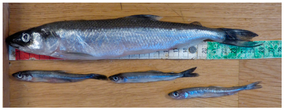
Figure 2.
Map of Lake Mjøsa with transects for echosounding in May 2024 between Brumunddal and Hamar in Furnesfjorden.
Figure 2.
Map of Lake Mjøsa with transects for echosounding in May 2024 between Brumunddal and Hamar in Furnesfjorden.
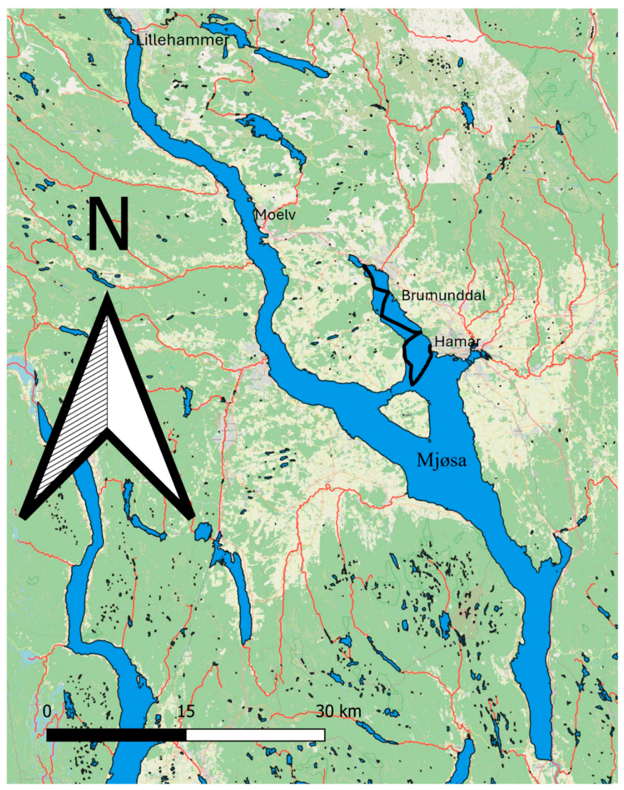
Figure 3.
Estimated pelagic biomass in different years in Lake Mjøsa.
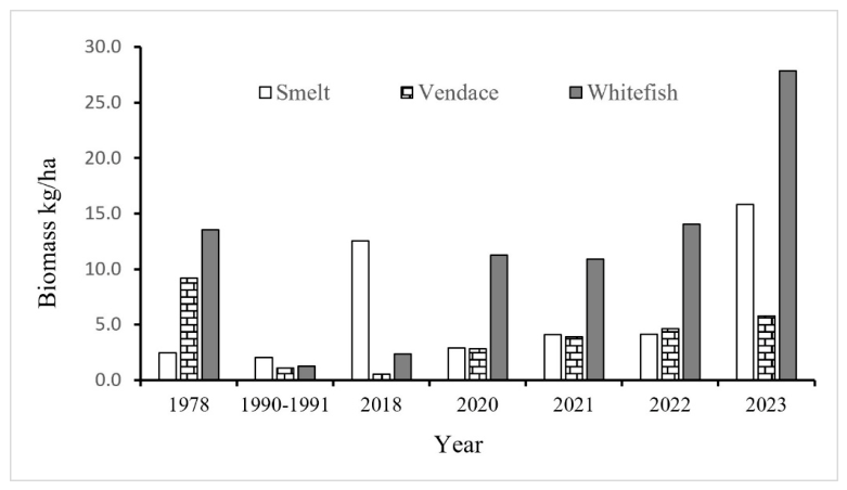
Figure 4.
Echogram from Furnesfjorden on 20 May 2021.
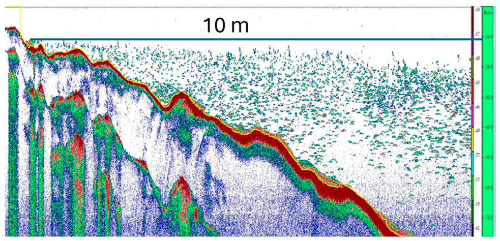
Figure 5.
Length distribution of fish recorded by means of echosounding in Furnesfjorden 20 May 2021.
Figure 5.
Length distribution of fish recorded by means of echosounding in Furnesfjorden 20 May 2021.
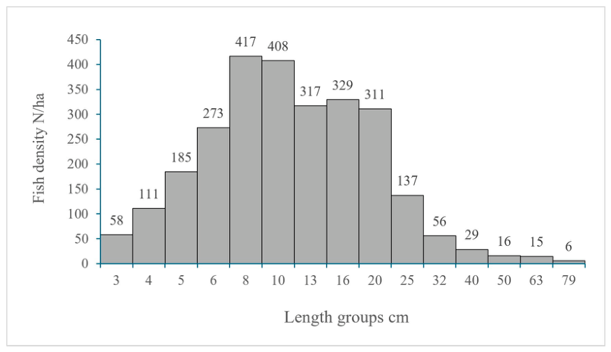
Figure 6.
Length distribution in smelt catches from spawning grounds in Furnesfjorden in different years.
Figure 6.
Length distribution in smelt catches from spawning grounds in Furnesfjorden in different years.
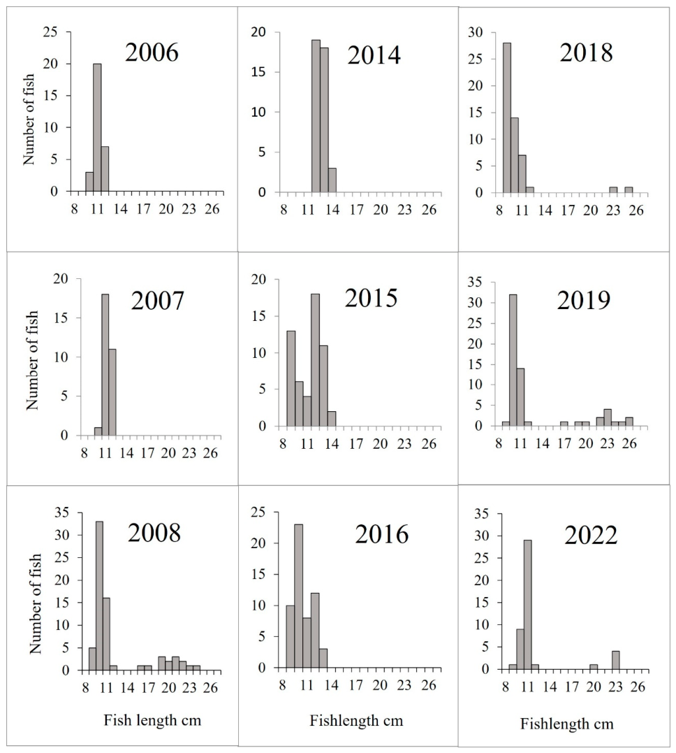
Figure 7.
Age distribution in smelt catches from spawning grounds in Furnesfjorden in different years.
Figure 7.
Age distribution in smelt catches from spawning grounds in Furnesfjorden in different years.
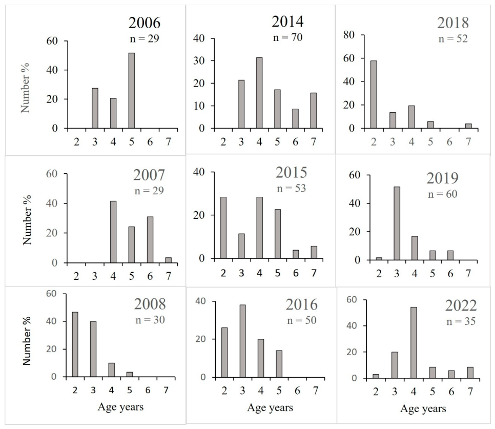
Figure 8.
Mean lengths of normal smelt females and males combined from 1900-1904 and 1978-1980, and mean lengths of males from 1978-1980 and 2006-2022.
Figure 8.
Mean lengths of normal smelt females and males combined from 1900-1904 and 1978-1980, and mean lengths of males from 1978-1980 and 2006-2022.
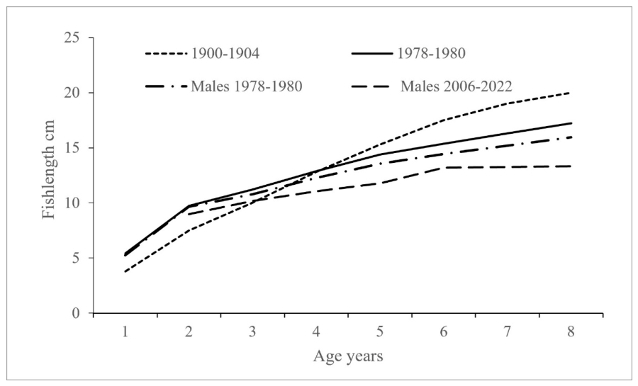
Figure 9.
Observed year-class distribution, estimated expected year-class distribution and relative year-class strength in smelt samples from 1980.
Figure 9.
Observed year-class distribution, estimated expected year-class distribution and relative year-class strength in smelt samples from 1980.
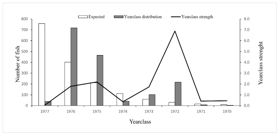
Figure 10.
Relative year-class strength in smelt samples from 1980 plotted on July air temperature.
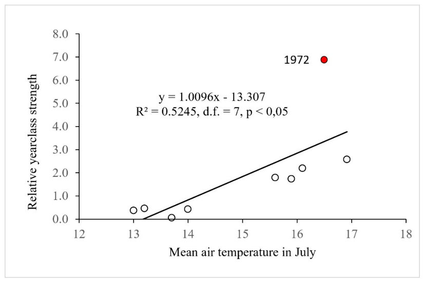
Figure 11.
Estimated relative strength of year-classes 2001 to 2020 (no data achieved for the 2007 year-class).
Figure 11.
Estimated relative strength of year-classes 2001 to 2020 (no data achieved for the 2007 year-class).
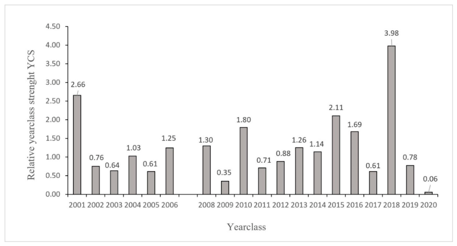
Figure 12.
Mean length of three species of Cladocera plotted on pelagic fish density in the 17 studied lakes (after Linløkken [44]).
Figure 12.
Mean length of three species of Cladocera plotted on pelagic fish density in the 17 studied lakes (after Linløkken [44]).
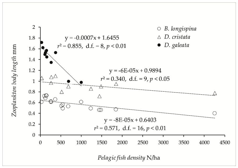
Figure 13.
Catch per net effort (fish/net night) reported by net fishermen, after Statsforvalteren [31].
Figure 13.
Catch per net effort (fish/net night) reported by net fishermen, after Statsforvalteren [31].
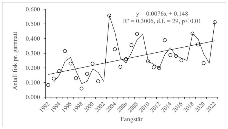
Table 1.
Estimated density (95% C.I.) and biomass in Furnesfjorden in May 2021 og 2024. Biomass is estimated by means of a model given in Supporting tables 1AB.
Table 1.
Estimated density (95% C.I.) and biomass in Furnesfjorden in May 2021 og 2024. Biomass is estimated by means of a model given in Supporting tables 1AB.
| Period |
Density of 5-70 cm long fish N/ha |
Density of 5-13 cm long fish N/ha | Biomass of 5-13 cm long fish |
| 20 May 2021 14:00-17:30 | 2666 (2592-2741) | 1599 (1555-1644) | 4,5 kg/ha |
| 15 May 2024 17:00-19:00 | 1825 (1674-1976) | 1110 (997-1224) | 3,2 kg/ha |
Table 3.
Linear model of normal smelt (< 15 cm) length, with Age and catch year as predictors (R2 = 0,77, d.f. = 375, p < 0,001).
Table 3.
Linear model of normal smelt (< 15 cm) length, with Age and catch year as predictors (R2 = 0,77, d.f. = 375, p < 0,001).
| Age/Growth year | Estimate | Standard error | t- verdi | p |
| 2+ 2005 | 77.617 | 1.770 | 43.86 | < 0,001 |
| Ln (Age) | 22.093 | 1.023 | 21.59 | < 0,001 |
| Growth year 2006 | -0.716 | 1.528 | -0.47 | > 0,05 |
| Growth year 2007 | -0.469 | 1.573 | -0.298 | > 0,05 |
| Growth year 2013 | 7.616 | 1.294 | 5.89 | < 0,001 |
| Growth year 2014 | 4.636 | 1.355 | 3.42 | < 0,001 |
| Growth year 2015 | -0.388 | 1.379 | -0.28 | > 0,05 |
| Growth year 2017 | -5.797 | 1.432 | -4.05 | < 0,001 |
| Growth year 2018 | -4.677 | 1.379 | -3.39 | < 0,001 |
| Growth year 2021 | -3.878 | 1.511 | -2.57 | < 0,05 |
Table 4.
Annual survival (S) and instantan mortality (Z) estimated for smelt caught in different years.
Table 4.
Annual survival (S) and instantan mortality (Z) estimated for smelt caught in different years.
| 1979 | 1980 | 2007 | 2008 | 2014 | 2015 | 2016 | 2018 | 2019 | 2022 | |
| Annual survival S | 0.64 | 0.68 | 0.50 | 0.42 | 0.57 | 0.65 | 0,45 | 0.45 | 0,41 | 0,38 |
| ± 95% C.L. | 0,02 | 0,013 | 0,33 | 0,14 | 0,09 | 0,08 | 0,12 | 0,12 | 0,10 | 0,15 |
| Instant mortality Z | 0.44 | 0.38 | 0,69 | 0.87 | 0.55 | 0.44 | 0.81 | 0.81 | 0,90 | 0,97 |
Table 5.
Life history tables for smelt based on data from Sandlund, Klyve [5] Sandlund, Næsje [27] (left) and from data sampled after 2006 in addition to Eikland, Gjelland [41](right) with estimation of biomass (B) and production (P) in the age groups 1 – 7 (N’ og B’, density and biomass at the start and end of season).
Table 5.
Life history tables for smelt based on data from Sandlund, Klyve [5] Sandlund, Næsje [27] (left) and from data sampled after 2006 in addition to Eikland, Gjelland [41](right) with estimation of biomass (B) and production (P) in the age groups 1 – 7 (N’ og B’, density and biomass at the start and end of season).
|
Smelt, Mjøsa 1980 |
NM | WM | BM | P | Smelt, Mjøsa 2023 | NM | WM |
BM |
P | ||||||||||
| Adjusted | Tot./ha = | 244 | 6,1 | 1,49 | 0,61 | Adjusted | Tot./ha = |
3160 |
3,3 | 10,4 | 6,5 | ||||||||
| Age | L, cm | W, g | G | M | N’ | N | B’ | BM | P | L, cm | W, g | G | M | N’ | N | B’ | BM | P | |
| 1 | 5.3 | 0.62 | 91 | 0.06 | 4.8 | 0.45 | 1868 | 0.85 | |||||||||||
| 1.91 | 0.13 | 85 | 0.138 | 0.26 | 2.06 | 0.24 | 1653 | 2.102 | 4.32 | ||||||||||
| 1+ | 9.7 | 4.20 | 80 | 0.34 | 9.2 | 3.55 | 1463 | 5.20 | |||||||||||
| 0.26 | 0.49 | ||||||||||||||||||
| 2 | 9.7 | 4.20 | 62 | 0.26 | 9.2 | 3.55 | 897 | 3.19 | |||||||||||
| 0.34 | 0.13 | 58 | 0.289 | 0.10 | 0.29 | 0.24 | 793 | 3.268 | 0.96 | ||||||||||
| 2+ | 10.8 | 5.90 | 54 | 0.32 | 10.1 | 4.77 | 702 | 3.35 | |||||||||||
| 0.26 | 0.49 | ||||||||||||||||||
| 3 | 10.8 | 5.90 | 42 | 0.25 | 10.1 | 4.77 | 430 | 2.05 | |||||||||||
| 0.41 | 0.13 | 39 | 0.286 | 0.12 | 0.21 | 0.24 | 381 | 2.021 | 0.43 | ||||||||||
| 3+ | 12.3 | 8.90 | 37 | 0.33 | 10.8 | 5.90 | 337 | 1.99 | |||||||||||
| 0.26 | 0.49 | ||||||||||||||||||
| 4 | 12.3 | 8.90 | 29 | 0.25 | 10.8 | 5.90 | 207 | 1.22 | |||||||||||
| 0.32 | 0.13 | 27 | 0.280 | 0.09 | 0.23 | 0.24 | 183 | 1.207 | 0.27 | ||||||||||
| 4+ | 13.6 | 12.22 | 25 | 0.31 | 11.6 | 7.39 | 162 | 1.20 | |||||||||||
| 0.26 | 0.49 | ||||||||||||||||||
| 5 | 13.6 | 12.22 | 19 | 0.24 | 11.6 | 7.39 | 99 | 0.73 | |||||||||||
| 0.22 | 0.24 | 17 | 0.235 | 0.053 | 0.79 | 0.24 | 88 | 0.963 | 0.76 | ||||||||||
| 5+ | 14.6 | 15.29 | 15 | 0.23 | 14.9 | 16.31 | 78 | 1.27 | |||||||||||
| 0.26 | 0.49 | ||||||||||||||||||
| 6 | 14.6 | 15.29 | 12 | 0.18 | 14.9 | 16.31 | 48 | 0.78 | |||||||||||
| 0.13 | 0.24 | 10 | 0.170 | 0.022 | -0.36 | 0.24 | 42 | 0.574 | -0,21 | ||||||||||
| 6+ | 15.2 | 17.37 | 9 | 13.3 | 11.39 | 37 | 0.42 | ||||||||||||
| 0.00 | 0.26 | 0.49 | |||||||||||||||||
| 7 | 15.2 | 17.37 | 7 | 0.12 | 13.3 | 11.39 | 23 | 0.26 | |||||||||||
| -0.42 | 0.24 | 6 | 0.089 | -0.037 | 0.00 | 0.24 | 20 | 0.230 | 0.00 | ||||||||||
| 7+ | 13.3 | 11.39 | 6 | 13.3 | 11.39 | 18 | |||||||||||||
| Totalt | 244 | 1.487 | 0.605 | 3160 | 10.4 | 6.5 | |||||||||||||
Table 6.
Mean number of hours spent to land a brown trout by rod and reel fishing in Brumunda and Lake Mjøsa and mean fish weight in different time periods, after Qvenild and Nashoug [51] and Norum and Thorkildsen [32].
| Location | Mean | 1985 | 1992-2022 | 2007-2009 |
| Mean (Min-Max) | Annual mean | |||
| Brumunda | Hours per fish | 5,1 | - | 2,7-3,5 |
| Weight (kg) | 0,56 | - | 1,6-1,7 | |
| Mjøsa | Hours per fish | 12,0 | 5,7 (2,4-9,7) | - |
| Weight (kg) | 1,26 | 1,75 (1,1-2,7) | - |
Disclaimer/Publisher’s Note: The statements, opinions and data contained in all publications are solely those of the individual author(s) and contributor(s) and not of MDPI and/or the editor(s). MDPI and/or the editor(s) disclaim responsibility for any injury to people or property resulting from any ideas, methods, instructions or products referred to in the content. |
© 2026 by the authors. Licensee MDPI, Basel, Switzerland. This article is an open access article distributed under the terms and conditions of the Creative Commons Attribution (CC BY) license (http://creativecommons.org/licenses/by/4.0/).
Copyright: This open access article is published under a Creative Commons CC BY 4.0 license, which permit the free download, distribution, and reuse, provided that the author and preprint are cited in any reuse.