

Submitted:
25 August 2026
Posted:
26 August 2026
You are already at the latest version
Abstract
Fluorescence time–lapse microscopy is a fundamental tool for investigating dynamic cellular processes, yet automatic cell detection and temporal signal extraction remain strongly dependent on intensity–driven thresholds and rigid decision rules. Such approaches may become unstable in the presence of noise, photobleaching, overlapping structures, and intrinsic biological variability. In this work, we introduce an uncertainty–aware computational framework that preserves the classical analysis workflow—temporal projection, peak detection, and region–of–interest (ROI) signal extraction—while extending it through neutrosophic morphological enhancement. The proposed implementation emphasizes practical reproducibility and flexibility: the analysis pipeline can automatically operate on heterogeneous inputs, including single images, temporal projections, full 3D stacks, or image sequences, while maintaining consistent detection parameters across classical and neutrosophic processing. By spatially flattening the image stack and enhancing the resulting activity landscape through neutrosophic morphology, the framework explicitly models reliable information, ambiguity, and background contributions, allowing weak but spatially coherent structures to emerge as stable candidates for detection. Beyond detection, the method extracts temporal ROI signals and provides detailed visualization and computational reporting, enabling a deeper interpretation of dynamic cellular behaviour. The framework remains fully compatible with standard fluorescence analysis pipelines while improving robustness, interpretability, and reproducibility under challenging imaging conditions, offering a principled extension for analysing uncertain or borderline cellular signals in fluorescence time–lapse microscopy.
Keywords:
fluorescence microscopy
; time-lapse imaging
; neutrosophic morphology
; automatic cell detection
; peak detection
; ROI signal extraction
; uncertainty-aware image analysis
; calcium imaging
; computational pipeline
1. Introduction
Fluorescence microscopy has become a key technique in modern biological and biomedical research [8], enabling the visualization and quantitative analysis of dynamic cellular processes with high spatial and temporal resolution. The range of observable spatiotemporal phenomena has been further expanded by advanced fluorescence microscopy techniques [6] and by fluorescent protein tools that support dynamic monitoring of molecular processes in living cells [5]. In fluorescence imaging, specific cellular components are selectively labeled with fluorophores that emit light at longer wavelengths when excited by an external illumination source.
Fluorescence time–lapse microscopy captures the temporal evolution of intracellular activity at the single–cell level or across cell populations by acquiring sequences of fluorescence images over time. It is therefore widely used to investigate intracellular signaling processes, particularly calcium dynamics. Calcium imaging provides a sensitive readout of intracellular signaling pathways and is broadly employed in the study of neuronal and glial activity [7]. In particular, time–lapse fluorescence microscopy is commonly applied to intracellular calcium signaling in astrocytes and other cell types, providing insights into complex spatiotemporal pathways underlying both physiological and pathological processes [9]. Astrocytes are now well established as active participants in neural information processing, engaging in bidirectional communication with neurons and contributing to network–level interactions [4].
Despite its versatility, fluorescence time–lapse microscopy is intrinsically affected by multiple sources of uncertainty. Fluorescence emission arises from stochastic photon–generation processes, and the resulting signals are often weak, especially when low excitation intensities are used to limit photobleaching and phototoxic effects. Consequently, acquired image sequences frequently exhibit low signal–to–noise ratios, spatially heterogeneous background fluorescence, and gradual intensity drifts over time. Moreover, cellular structures are rarely sharply delineated: cells often appear as diffuse and partially overlapping regions, with boundaries that are difficult to define in a crisp and unambiguous manner.
From a technological perspective, continuous improvements in temporal resolution have enabled the investigation of fast cellular and developmental processes [13]. Recent advances include high–speed and large–volume imaging techniques, such as multi–focus light–field microscopy [16], as well as automated electronic solutions designed to enhance the robustness and reproducibility of optical measurements [12]. In parallel, portable and low–cost fluorescence analysis systems have broadened the accessibility of time–lapse fluorescence methodologies in biological and environmental monitoring contexts [14].
Automatic cell detection and temporal signal extraction are central components of fluorescence time–lapse microscopy analysis pipelines. Most approaches rely on deterministic image–processing techniques, including intensity thresholding, local maxima detection, and predefined regions of interest (ROIs), to identify candidate cellular regions and extract corresponding fluorescence signals [15]. While effective under favorable imaging conditions, these methods often exhibit limited robustness in realistic experimental settings, where noise, uneven illumination, photobleaching, and overlapping cellular structures are commonly present.
A key methodological limitation of classical image–processing pipelines lies in their inherently crisp nature, which forces uncertain or ambiguous information into deterministic categories. Mathematical morphology provides a rigorous framework for shape–based image analysis through operators such as dilation and erosion and is therefore widely adopted in classical pipelines [10]. However, classical morphological approaches do not explicitly model uncertainty, and ambiguous structures are frequently suppressed by hard decision rules.
Earlier uncertainty–aware theories, such as intuitionistic fuzzy sets, extended classical fuzzy logic by incorporating degrees of truth and falsity, but did not explicitly consider indeterminacy as an independent concept [3]. Neutrosophic set theory, introduced by Smarandache, further generalizes these approaches by explicitly modelling degrees of truth, indeterminacy, and falsity [11], thereby providing a richer mathematical framework for representing uncertain and ambiguous information.
Neutrosophic image processing has recently enabled computational implementations of neutrosophic morphological operators. In particular, the Python class NSmorph provides implementations of neutrosophic dilation, erosion, opening, and closing, facilitating the integration of neutrosophic theory into practical image–processing workflows [2]. Nevertheless, the potential of neutrosophic morphology in the context of dynamic fluorescence time–lapse microscopy remains largely unexplored.
At the same time, automated analysis pipelines for fluorescence time–lapse microscopy that combine temporal projection with peak detection continue to rely primarily on deterministic decision rules to localize candidate regions and extract fluorescence signals. Under non–ideal imaging conditions, such pipelines tend to force weak or uncertain structures into binary classifications (e.g., cell versus background, signal versus noise), leading to the premature loss of borderline but potentially meaningful activity patterns.
In this work, we propose a principled neutrosophic generalization of classical peak–based workflows by explicitly modelling three complementary components: reliable information (truth), uncertainty (indeterminacy), and non–relevant or artifactual information (falsity). Rather than discarding ambiguous signals through hard thresholding, the proposed framework retains and characterizes uncertainty, producing an enhanced spatial activity representation on which classical peak detection can operate unchanged.
Building on this perspective, we integrate neutrosophic morphology into an automated and reproducible computational pipeline for cell detection and temporal signal extraction in fluorescence time–lapse microscopy of astrocytes. The implementation is designed to operate transparently on heterogeneous input modalities (single images, temporal projections, full 3D stacks, or ordered image sequences), while preserving a unified detection strategy shared by classical and neutrosophic processing. Representative code fragments are included throughout the manuscript to document the main computational steps and to promote reproducibility. Classical deterministic approaches are recovered as special cases of the proposed framework when the indeterminacy component is neglected, showing that the neutrosophic formulation complements—rather than replaces—existing methods, while improving robustness, interpretability, and computational transparency under challenging imaging conditions.
2. Theoretical Background: Neutrosophic Modeling
Automatic cell detection in fluorescence time–lapse microscopy is typically performed by identifying local intensity maxima and subsequently defining Regions of Interest (ROIs) with fixed geometric shapes. In classical analysis pipelines, both peak detection and ROI definition rely on crisp decision rules, which makes the overall workflow sensitive to noise, uneven background fluorescence, partially overlapping cellular structures, and the tuning of algorithmic parameters.
Within the neutrosophic framework, fluorescence images are modeled as neutrosophic images (see [1,2]), where uncertainty and ambiguity are explicitly represented rather than implicitly discarded. This section introduces the theoretical foundations underlying the proposed neutrosophic enhancement strategy and clarifies how these concepts interface with the computational pipeline described later.
A key enabling component of the framework is the Python class NSmorph, which implements neutrosophic morphological operators such as dilation, erosion, opening, and closing. The class represents images as triplets encoding truth, indeterminacy, and falsity components, allowing classical morphological transformations to be extended into an uncertainty–aware domain. Importantly, NSmorph supports multiple input modalities—including image files, NumPy arrays, and existing neutrosophic instances—which facilitates seamless integration into heterogeneous fluorescence imaging workflows [2]. In the present pipeline, neutrosophic enhancement is applied to temporally aggregated fluorescence data prior to peak detection.
2.1. Neutrosophic Representation of Fluorescence Images
Let be a discrete spatial domain. In practical imaging scenarios, U is typically a finite rectangular pixel grid of the form , representing the spatial support of a fluorescence image. A neutrosophic image is defined as a triplet
where the three components are independent functions assigning to each spatial location the degree of reliable (truth) information, the degree of indeterminacy (uncertainty or ambiguity), and the degree of non–membership (falsity, typically associated with background or artifacts), respectively. The three components are conceptually independent; therefore no normalization constraint is imposed on their sum, which simply satisfies
This representation generalizes both crisp (binary) and fuzzy (single–membership) models by preserving uncertainty as an explicit and independent component.
In practice, a neutrosophic image is not given a priori but is constructed from a classical grayscale fluorescence image (or from a temporally flattened projection). Figure 1 illustrates the transformation from the original fluorescence image to the three neutrosophic components , , and , which together form the neutrosophic image .
Let denote a normalized fluorescence image. The associated neutrosophic image is obtained by generating the three degree functions , and .
A widely adopted construction derives the truth component from a local mean intensity computed on a square neighbourhood of radius . More precisely, for every pixel and every , we define the square neighbourhood centered at with radius r as
and the corresponding local mean map
where the summation is restricted to valid pixels near image boundaries.
Let
The truth (membership) component is then obtained by min–max normalization:
with the convention whenever . Operationally, emphasizes spatially coherent bright regions while attenuating isolated pixel fluctuations.
Indeterminacy is constructed by measuring local instability through the deviation from the local mean,
Let
The indeterminacy channel is then defined as
with if . Large values of typically correspond to pixels whose intensity is locally ambiguous, for instance due to noise, heterogeneous background, overlap between structures, or weak spatial contrast.
A computationally convenient choice for the falsity channel, also adopted in the NSmorph framework, is the complement of the truth degree:
Under this convention, dark or background–dominated regions exhibit high , whereas coherent bright structures exhibit low . The indeterminacy component remains independently defined and therefore the triplet does not satisfy any fixed–sum constraint.
In the computational implementation adopted in this work, the construction of the neutrosophic image from a normalized fluorescence map is performed through the constructor of the NSmorph class, which internally computes the three components , and according to the local mean and local deviation scheme described below. This ensures a direct correspondence between the theoretical formulation and the implemented pipeline.
Within fluorescence imaging, the three channels admit a direct interpretation: highlights spatially coherent active regions, preserves uncertainty associated with weak or ambiguous structures, and captures non–relevant background contributions. This triplet representation provides the starting point for neutrosophic morphological operators, which primarily reshape the truth component while maintaining an explicit representation of uncertainty through .
2.2. Peak Enhancement via Neutrosophic Morphology
To improve the robustness of peak detection, neutrosophic morphological operators can be applied to [1,2]. Let B be a structuring element. Neutrosophic dilation and erosion act component-wise on , reinforcing spatially coherent structures in the truth component while attenuating non–relevant fluctuations and stabilizing ambiguous patterns.
Denote by the neutrosophic dilation of . The resulting transformed neutrosophic image is
In the computational framework adopted here, neutrosophic opening and closing are applied sequentially through the NSmorph class to generate an enhanced activity landscape. The enhanced truth component is then used as the primary map for peak detection. This design preserves the classical peak detection algorithm and its parameters while replacing the input with a morphologically stabilized representation that is less sensitive to local noisy maxima.
2.3. Neutrosophic Peaks and Peak Detection
A candidate fluorescence peak at location can be conceptualized as a neutrosophic peak
where measures the degree to which u behaves as a biologically meaningful local maximum, reflects ambiguity (e.g., competing nearby maxima or low spatial contrast), and quantifies non–relevance (e.g., background–driven maxima).
Operationally, peak candidates in this work are detected as local maxima of the enhanced truth map . The indeterminacy and falsity components provide a theoretical layer for interpreting ambiguous detections; however, the computational pipeline intentionally focuses on the truth component to maintain stability and comparability with classical workflows.
It is important to emphasize that the peak detection algorithm itself remains identical in both the classical and neutrosophic pipelines. No modification is introduced at this stage in terms of algorithmic logic or parameterization. Consequently, any differences observed in detection results arise solely from the different representations of the input map used during peak detection.
2.4. ROI Definition and Interface with the Adopted Pipeline
Given peak coordinates, classical pipelines define ROIs using predetermined geometric shapes (commonly circular masks) and extract temporal signals by aggregating pixel intensities within each ROI. A full neutrosophic generalization would model an ROI as a neutrosophic region
thereby allowing soft boundaries and explicitly representing uncertain pixels near ROI borders. This viewpoint is particularly useful for interpreting dense or ambiguous cellular fields.
In the present implementation, ROIs are intentionally defined as crisp circular masks centered at detected peaks, and the temporal signal is computed as the mean intensity within each ROI. This choice preserves the standard ROI geometry used in classical workflows, ensuring that differences with respect to deterministic pipelines can be attributed exclusively to the neutrosophic enhancement stage rather than to downstream processing changes.
2.5. Neutrosophic Temporal Signals (Conceptual Extension)
For completeness, we outline the natural neutrosophic extension of ROI–based signal extraction. Let denote the neutrosophic image at time t and a neutrosophic ROI. A neutrosophic temporal signal can then be defined as
with components computed via weighted aggregations, for example
Here, represents reliable fluorescence activity, quantifies temporal uncertainty, and captures background contributions and imaging artifacts. The classical temporal signal is recovered by adopting crisp ROI membership and neglecting the indeterminacy and falsity components.
2.6. Neutrosophic Activity and Event Characterization (Conceptual Extension)
Neutrosophic temporal signals enable a principled characterization of cellular activity and signaling events. For instance, an event at time may be associated with an increase in under bounded uncertainty:
More generally, an overall neutrosophic activity descriptor
can be obtained by aggregating over the observation window. This formulation generalizes binary activity labels by retaining borderline and ambiguous cases as first–class objects rather than forcing them into rigid categories.
3. Methods
3.1. Overview of the Computational Pipeline
The proposed computational pipeline preserves the conceptual structure commonly adopted in classical fluorescence time–lapse microscopy analysis, namely temporal projection, peak detection, and region–of–interest (ROI) signal extraction. The standard workflow is extended by the inclusion of a neutrosophic morphological enhancement step prior to peak detection, while all downstream stages are intentionally kept unchanged in order to enable a controlled comparison with classical approaches.
A distinctive feature of the implementation is its ability to operate transparently on heterogeneous input modalities. The pipeline accepts single images, temporal projections, full three–dimensional stacks, or image sequences, automatically adapting the preprocessing stage while preserving identical detection parameters. This design promotes reproducibility and facilitates integration into existing fluorescence analysis workflows.
The pipeline consists of the following main steps:
- (i)
- temporal flattening of the image stack,
- (ii)
- neutrosophic morphological enhancement of the flattened map,
- (iii)
- peak detection on the enhanced map,
- (iv)
- ROI–based temporal signal extraction from the original stack, and
- (v)
- generation of diagnostic outputs and computational reports.
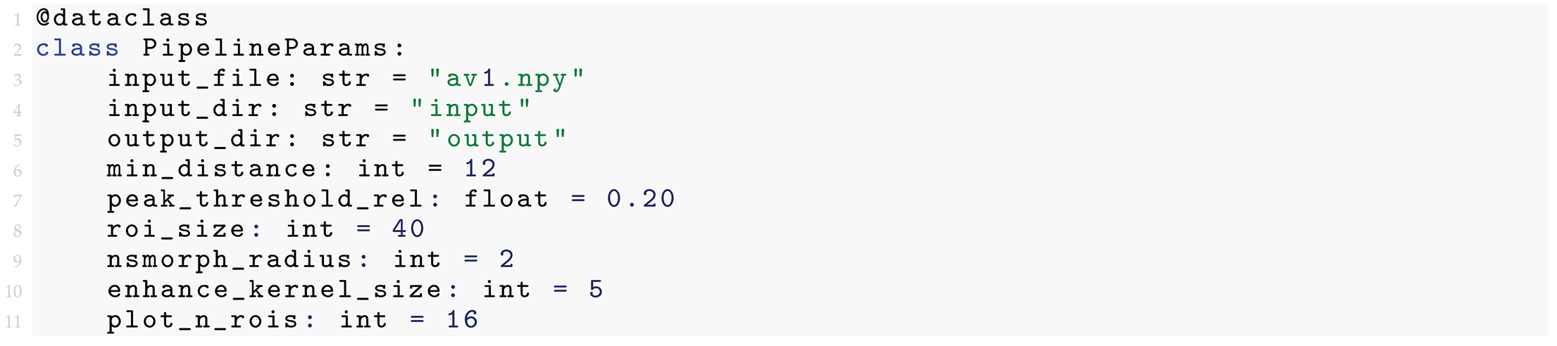
All processing parameters are centrally controlled through a dedicated configuration structure (PipelineParams), ensuring transparency, interpretability, and reproducibility of the computational results.
3.2. Input Data and Temporal Flattening
The framework supports multiple input modalities in order to facilitate integration with heterogeneous experimental workflows. Accepted inputs include single fluorescence images, temporally flattened projections, three–dimensional NumPy arrays (.npy stacks), and directories containing ordered image sequences. When a directory is provided, images are automatically sorted and assembled into a time–lapse stack; when a precomputed projection is detected, it can be used directly for peak detection while preserving the original stack for temporal signal extraction.
All inputs are internally converted into a canonical stack representation , where T denotes the number of frames and the spatial resolution. This normalization step decouples data acquisition from algorithmic processing and allows identical detection parameters to be applied across heterogeneous datasets.
Temporal flattening is performed by summation,
which emphasizes spatial locations exhibiting sustained or recurrent fluorescence activity while attenuating transient fluctuations. If a precomputed projection is explicitly provided, it is used directly; otherwise the projection is computed from the stack.

The flattened projection is stored as a diagnostic reference image to ensure reproducibility of the detection stage:

This design guarantees that peak detection always operates on a well–defined spatial activity map independently of the original data modality.
3.3. Neutrosophic Morphological Enhancement
Neutrosophic morphological enhancement constitutes the core uncertainty–aware preprocessing stage of the pipeline. Starting from the flattened activity map , the image is first normalized to the unit interval and then mapped to a neutrosophic image through the constructor of the NSmorph class. This step produces an initial neutrosophic representation
where the three components encode, respectively, reliable intensity evidence, local ambiguity, and non–relevant/background contributions.

In the subsequent enhancement stage, we do not operate on the grayscale map directly, but rather on the neutrosophic image itself. In particular, we apply a neutrosophic opening followed by a neutrosophic closing respect to the same neutrosophic kernel (or structuring element) which, in this case, is a small cross, through the corresponding methods of NSmorph. Conceptually, opening (erosion followed by dilation) tends to suppress small and isolated bright structures, thereby removing spurious maxima likely caused by noise; closing (dilation followed by erosion) tends to fill small gaps and stabilize spatially coherent domains, yielding smoother and more connected activity regions. Within the neutrosophic setting, these operators are applied within the triplet representation, so that the enhancement of coherent structures is coupled with an explicit handling of local indeterminacy.
Denoting by
the neutrosophic opening and closing of the neutrosophic image with respect to the neutrosophic kernel , respectively, then the filtered neutrosophic image is
which, translated in Python code by the NSmorph class, means

The enhanced activity map used for peak detection is obtained by extracting the truth component of the filtered neutrosophic image via the accessor getM(). Therefore, the enhanced_map in the implementation coincides with the updated truth degree , that is in our code:

This design makes the comparison with classical pipelines fully controlled: the downstream peak detector operates on a standard numerical array, and the only difference with respect to the classical workflow lies in replacing the raw flattened projection with the morphologically stabilized truth component extracted from the neutrosophic representation.
3.4. Peak Detection
Candidate cellular locations are identified as local maxima of the enhanced truth map produced by the neutrosophic enhancement stage. Peak detection relies on a classical local–maxima strategy, ensuring full methodological compatibility with standard fluorescence analysis workflows.
An adaptive threshold proportional to the dynamic range of the enhanced map is employed to maintain robustness across datasets characterized by different intensity scales:

The adaptive formulation avoids fixed thresholds and stabilizes detection under heterogeneous illumination conditions. Importantly, the peak detection algorithm and its parameters are identical to those used in classical pipelines; only the input representation differs.
3.5. ROI Definition and Temporal Signal Extraction
For each detected peak, a circular region of interest (ROI) is defined and temporal fluorescence signals are extracted from the original stack. Let denote the circular ROI centered at the i–th detected peak. The temporal signal is computed as
where averaging is restricted to pixels belonging to a circular mask.
Operationally, each ROI is implemented by cropping an patch with and applying a circular mask of radius . Boundary conditions are handled by consistently cropping both patch and mask near image borders.

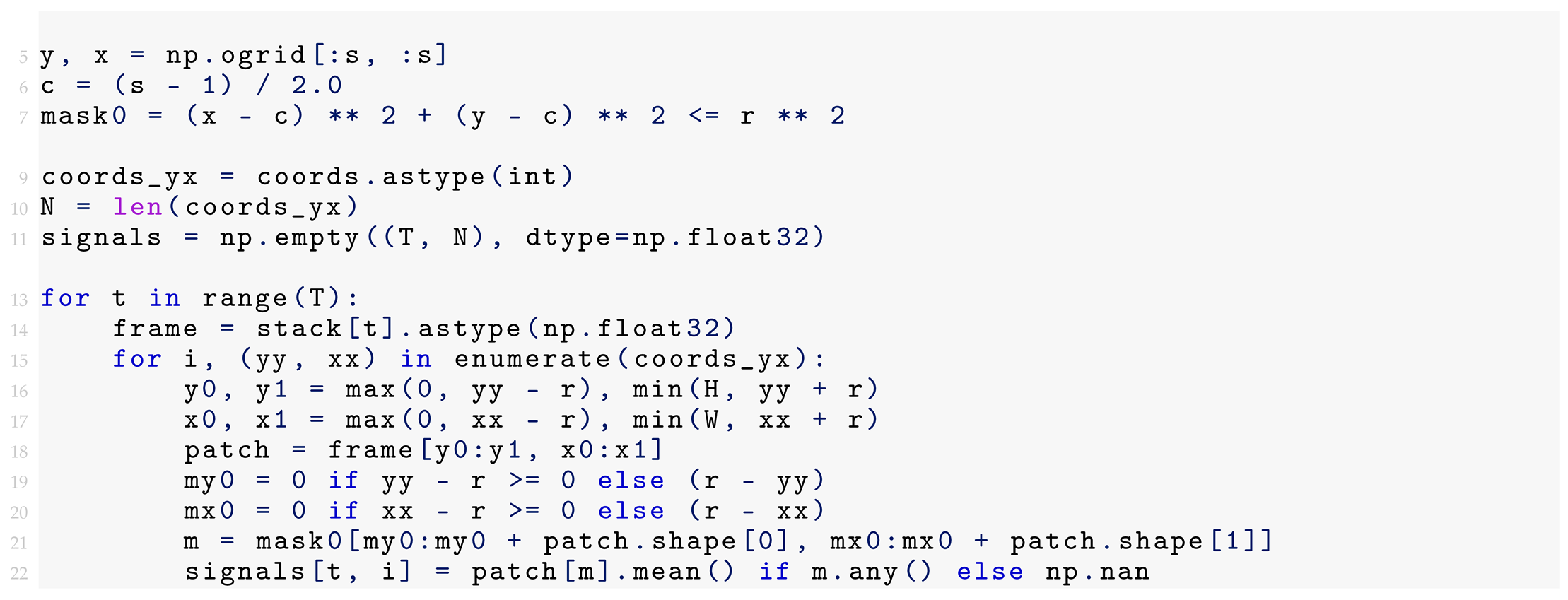
The extracted temporal signals form a matrix of size , preserving strict compatibility with classical circular ROI extraction while providing robust treatment of image boundaries.
3.6. Implementation and Diagnostic Outputs
The complete workflow is orchestrated by the function run_pipeline, which integrates neutrosophic enhancement, peak detection, and ROI–based signal extraction into a unified computational procedure. Given an input stack and a configuration structure, the function returns detected ROI coordinates, temporal signals, their headers, and the enhanced map used for peak detection.

The enhanced map is exported as a diagnostic image, while ROI signals are stored as a CSV file:

In addition to numerical outputs, the framework produces visualization artifacts aimed at facilitating qualitative validation, including peak overlays on the enhanced map, three–dimensional representations of the activity landscape, selected ROI overlays, and temporal signal plots whenever temporal information is available.
A structured computational report summarizing input characteristics, number of detected ROIs, signal matrix dimensions, and execution statistics is generated at the end of each run and stored within the output directory:

4. Computational Framework
While the previous section focuses on the algorithmic methodology, this section describes the architectural design and implementation strategy of the computational framework that bridges neutrosophic modeling with practical fluorescence time–lapse microscopy analysis. The framework has been conceived as a modular and extensible Python workflow aimed at enabling uncertainty–aware processing while preserving full compatibility with classical image analysis pipelines. Particular attention has been devoted to separation of concerns, reproducibility, and transparency of the computational workflow.
4.1. Modular Architecture and Data Flow
The implementation follows a modular architecture in which each processing stage corresponds to a clearly defined functional block. Temporal flattening, neutrosophic enhancement, peak detection, ROI extraction, signal computation, and diagnostic visualization are implemented as independent yet interoperable components. This separation allows individual stages to be modified or replaced without affecting the overall structure of the pipeline, facilitating experimentation with alternative processing strategies.
Internally, all operations are performed on multidimensional NumPy arrays, providing a unified numerical representation across heterogeneous data sources. Inputs such as single fluorescence images, temporally flattened projections, full three–dimensional stacks, NumPy arrays, or directories containing ordered image sequences are converted into a canonical representation before processing. By decoupling input handling from algorithmic logic, the framework ensures that downstream operations remain invariant with respect to the original data modality.
From a data–flow perspective, the pipeline can be interpreted as a sequence of transformations acting on progressively refined spatial representations: raw fluorescence intensities are aggregated into temporal projections, transformed into neutrosophically enhanced activity landscapes, and finally mapped into temporally resolved ROI signals suitable for quantitative analysis.
4.2. Input Normalization and Data Abstraction
At the architectural level, input handling is implemented as an abstraction layer that isolates data ingestion from the neutrosophic processing core. Rather than redefining preprocessing operations already described in Section 3, this layer provides a standardized interface through which heterogeneous datasets are converted into the internal stack representation used by the framework.

This design ensures that normalization, validation, and metadata extraction are performed consistently before entering the computational pipeline. By separating data acquisition from analysis logic, identical detection parameters can be applied across datasets originating from different experimental conditions, improving reproducibility and reducing implementation complexity.
4.3. Integration of the NSmorph Engine
The neutrosophic morphological enhancement stage relies on the NSmorph class, which serves as the core computational engine for uncertainty–aware image processing. Instead of operating on a single intensity channel, NSmorph maintains a triplet representation encoding truth, indeterminacy, and falsity components throughout the transformation process. Morphological operators such as opening and closing are applied component–wise, reinforcing spatially coherent structures while preserving information about ambiguous or low–contrast regions.
From a computational standpoint, the enhanced truth component produced by NSmorph remains fully compatible with classical processing routines. Peak detection algorithms therefore operate on a standard numerical array, allowing existing implementations to be reused without modification. This design embeds neutrosophic modeling into the preprocessing stage as a transparent extension rather than introducing an entirely new analytical workflow.
4.4. Neutrosophic Processing Core
The central execution layer integrates neutrosophic enhancement with classical peak detection and ROI extraction into a unified computational procedure. The pipeline orchestration is handled through a dedicated execution interface:

Within this architecture, neutrosophic modeling reshapes the spatial structure of the data without modifying downstream signal extraction logic. Classical pipelines therefore emerge naturally as limiting cases obtained by bypassing the enhancement stage, enabling direct comparisons between deterministic and uncertainty–aware processing strategies.
4.5. Parameter Management and Reproducibility
All algorithmic parameters are centralized within the PipelineParams configuration structure. Parameters controlling peak detection, ROI geometry, neutrosophic neighborhood size, and visualization behavior are stored in a single object, ensuring that the computational behavior of the pipeline is fully determined by a compact and reproducible configuration.
Centralized parameter management simplifies experimental evaluation by allowing systematic variation of individual parameters while maintaining a consistent processing environment. This design facilitates controlled comparisons between classical and neutrosophic pipelines without introducing confounding algorithmic differences.
4.6. Diagnostic Outputs and Visualization Strategy
Beyond numerical outputs, the framework produces a comprehensive set of diagnostic visualizations aimed at supporting interpretability and qualitative validation. These include enhanced activity maps, overlays of detected peaks, ROI selection masks, temporal signal plots, cumulative intensity histograms, and optional three–dimensional representations of the enhanced activity landscape.
The visualization strategy emphasizes transparency of the processing stages. Rather than treating image analysis as a purely numerical optimization problem, intermediate visual artifacts are generated to illustrate how neutrosophic enhancement reshapes the spatial organization of fluorescence data. In particular, the three–dimensional activity landscape provides an intuitive geometric interpretation of peak detection as the identification of dominant local maxima on an enhanced surface.
4.7. Execution Workflow and Output Generation
The computational workflow coordinates all processing stages and aggregates the resulting outputs through a structured export interface. Enhanced activity maps and ROI signals are exported using dedicated routines:

In addition to CSV tables of ROI traces, the framework generates structured textual reports summarizing dataset dimensions, processing parameters, detection statistics, and signal matrix characteristics. This layered output design facilitates integration with external statistical or visualization environments while maintaining full traceability of the computational workflow.
4.8. Design Philosophy: Compatibility with Classical Pipelines
A fundamental guiding principle of the framework is backward compatibility with classical fluorescence time–lapse analysis workflows. All downstream processing stages—peak detection, ROI definition, and signal extraction—are intentionally preserved. Classical pipelines can therefore be recovered simply by bypassing the neutrosophic enhancement stage.
This compatibility ensures that improvements observed in the results can be directly attributed to neutrosophic modeling rather than to unrelated algorithmic changes. More broadly, the framework demonstrates how uncertainty–aware image processing can be integrated into established analytical ecosystems without requiring substantial modifications to existing methodologies.
5. Results
This section presents qualitative and quantitative results obtained using the proposed neutrosophic analysis pipeline applied to fluorescence time–lapse microscopy data. Rather than focusing solely on detection performance, the results highlight how neutrosophic enhancement reshapes the spatial activity landscape and influences downstream temporal signal extraction.
5.1. Qualitative Visualization of the Detection Pipeline
Figure 2 shows a representative fluorescence frame characterized by heterogeneous background illumination and partially overlapping cellular structures.
Figure 3 presents the corresponding enhanced truth map obtained after neutrosophic morphological processing.
The enhancement stage produces a smoother and more structured spatial representation in which candidate cellular regions emerge as coherent activity domains. Instead of amplifying raw intensity variations, neutrosophic processing emphasizes morphological consistency, resulting in a stabilized activity landscape suitable for peak detection.
For an intuitive geometric interpretation, Figure 4 shows the enhanced truth map as a three–dimensional surface, where neutrosophic enhancement transforms the flattened projection into a smoother and more interpretable activity landscape. Peaks appear as dominant local maxima, highlighting the structural effect of neutrosophic morphology.
Peak detection results obtained with classical and neutrosophic pipelines are compared in Figure 5. The classical pipeline performs detection directly on the flattened projection, whereas the proposed framework operates on the neutrosophically enhanced landscape.
The classical pipeline produces a dense distribution of detections, many associated with background fluctuations or local intensity noise. In contrast, neutrosophic enhancement promotes spatial coherence, yielding a distribution of peaks that aligns more closely with visually identifiable activity regions.
5.2. ROI Selection and Temporal Signal Analysis
Figure 6 shows a subset of ROIs selected for temporal analysis. Circular masks are centered on detected peaks, maintaining strict compatibility with classical ROI extraction strategies while benefiting from improved spatial localization.
Temporal fluorescence signals extracted from representative ROIs are presented in Figure 7. The signals exhibit heterogeneous dynamics, including sustained activity patterns and transient fluctuations.
ROIs associated with spatially coherent structures tend to display smoother temporal profiles, whereas weaker detections exhibit lower amplitude variations. This behavior suggests that neutrosophic enhancement improves spatial localization, indirectly stabilizing temporal signal extraction without modifying downstream averaging procedures.
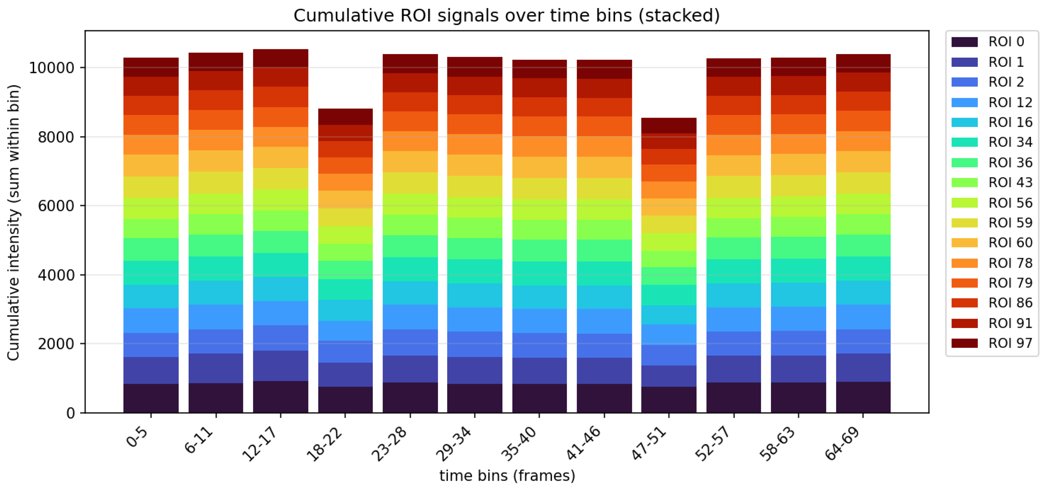
To analyze population–level trends, cumulative ROI signals aggregated over temporal bins are shown in Figure 8.
The cumulative representation highlights differences in global activity levels across ROIs. Regions identified after neutrosophic enhancement contribute more consistently across temporal bins, indicating that the framework favors spatially stable activity patterns rather than isolated noise-driven detections.
5.3. Quantitative Comparison of Detected Peaks
Beyond qualitative inspection, a clear quantitative difference emerges between classical and neutrosophic pipelines. Using identical detection parameters, the classical pipeline identifies 58 candidate peaks, whereas the neutrosophic pipeline detects 113 peaks.

Table 1.
Quantitative comparison between classical and neutrosophic detection pipelines.
| Pipeline | Detected Peaks (N) | Detection Strategy |
|---|---|---|
| Classical | 58 | Direct peak detection on the temporally flattened projection. |
| Neutrosophic | 113 | Peak detection performed on the neutrosophically enhanced truth map. |
This increase should not be interpreted as over–segmentation. Instead, the neutrosophic framework delays irreversible decisions by retaining ambiguous but spatially coherent structures through the indeterminacy component, allowing borderline activity regions to remain available for subsequent interpretation.
6. Discussion
The results presented in Section 5 provide both qualitative and quantitative evidence of the impact of neutrosophic modeling on fluorescence time–lapse microscopy analysis. Beyond the visual improvements observed in the enhanced activity landscapes, the proposed framework introduces a conceptual shift in the way cellular activity, uncertainty, and signal reliability are represented within automated analysis pipelines. In particular, the enhanced representations shown in Figures ?? and Figure 4 illustrate how neutrosophic morphology reshapes the spatial structure of temporally aggregated fluorescence data, producing smoother and more interpretable activity landscapes without modifying downstream detection logic.
6.1. Neutrosophic Interpretation of Detected Peaks
A key outcome of the comparative analysis is the marked difference in both the number and spatial organization of detected peaks obtained with classical and neutrosophic pipelines (Figure 5). While the classical approach identifies a limited set of candidate regions under identical detection parameters, the neutrosophic pipeline reveals a larger and more spatially coherent distribution of peaks.
This difference reflects a fundamental modeling distinction rather than a simple increase in detections. In classical pipelines, peak detection operates on a crisp intensity map, forcing each local structure into a binary decision between signal and background. Weak or ambiguous fluorescence regions are therefore removed during preprocessing. In contrast, the neutrosophic representation explicitly encodes uncertainty through the indeterminacy component , allowing morphologically consistent but low–contrast structures to be preserved during enhancement and subsequently detected as candidate peaks.
6.2. Role of Indeterminacy in Detection Stability
The explicit treatment of indeterminacy plays a central role in stabilizing peak detection. Classical pipelines implicitly treat uncertainty as noise to be suppressed, whereas neutrosophic enhancement propagates ambiguity through the preprocessing stage. As a result, ambiguous regions contribute to the enhanced truth component while retaining information about their uncertainty.
This behavior is visually reflected in the smoother activity landscape shown in Figure 4, where dominant maxima emerge as structured regions rather than isolated spikes. From a methodological perspective, peak detection becomes less sensitive to local intensity fluctuations and more dependent on spatial coherence encoded through neutrosophic morphological processing.
6.3. Implications for Temporal Signal Extraction
The benefits of neutrosophic enhancement extend beyond peak localization and directly influence ROI–based temporal signal extraction (Figure 6 and Figure 7). Improved spatial positioning of ROIs leads to temporal signals characterized by reduced background contamination and more stable temporal dynamics.
From a theoretical standpoint, a neutrosophic region of interest combined with a neutrosophic image sequence naturally yields a neutrosophic temporal signal
providing a structured representation of reliable activity, uncertainty, and background contributions. Although the present implementation computes classical intensity-based temporal signals, the improved spatial localization demonstrates that neutrosophic preprocessing can enhance downstream signal analysis without altering existing extraction algorithms.
6.4. Biological Interpretation and Population–Level Effects
From a biological perspective, the heterogeneous and continuous nature of cellular signaling aligns naturally with the neutrosophic framework. Regions exhibiting weak, intermittent, or spatially ambiguous activity are no longer excluded a priori, but are retained as candidate structures characterized by explicit levels of indeterminacy.
At the population level, the increased number of detected peaks should not be interpreted as a direct increase in distinct biological entities. Rather, it reflects the ability of the neutrosophic approach to capture subtle or partially overlapping activity patterns that deterministic pipelines tend to suppress. This behavior is particularly relevant in astrocytic networks, where signaling events often appear as diffuse and spatially extended phenomena.
6.5. Methodological Perspective and Limitations
From a methodological standpoint, the classical pipeline can be viewed as a limiting case of the neutrosophic framework in which indeterminacy is implicitly forced to zero and all decisions are reduced to crisp classifications. The proposed approach generalizes this setting by preserving ambiguous information and postponing strict decisions to later stages of analysis.
At the same time, the increased sensitivity of the neutrosophic pipeline introduces new challenges related to interpretation and validation. Not every detected peak necessarily corresponds to an independent biological structure, and future developments should incorporate temporal consistency criteria, clustering strategies, and validation against annotated datasets.
Importantly, the additional modeling expressiveness introduced by neutrosophic processing does not significantly increase computational complexity at the level of downstream analysis. By confining uncertainty–aware modeling to the enhancement stage and leveraging the modular NSmorph framework, the pipeline remains computationally efficient and fully compatible with standard peak detection and ROI–based signal extraction techniques.
7. Code and Data Availability
The computational pipeline developed and used in this work has been fully implemented in Python and is released as open–source software. The code is published under an open–source license and is available at the following GitHub repository: https://github.com/giorgionordo/pyNeutroDetection. The repository contains the complete implementation of the proposed neutrosophic morphological enhancement, peak detection, ROI–based temporal signal extraction, and diagnostic output generation. The public availability of the code is intended to support reproducibility, transparency, and further methodological extensions by the research community.
The fluorescence time–lapse microscopy data used in this study were generated as part of ongoing experimental activity and are not publicly available. However, the datasets can be made available by the authors upon reasonable request.
8. Conclusions and Perspectives
In this work, we introduced a neutrosophic generalization of automatic cell detection and temporal signal extraction for fluorescence time–lapse microscopy, combining uncertainty–aware modeling with a modular and reproducible computational framework. By representing fluorescence images through neutrosophic components, the proposed approach explicitly encodes reliable information (truth), ambiguity (indeterminacy), and non–relevant contributions (falsity), enabling a structured interpretation of complex and heterogeneous imaging data while maintaining compatibility with established analysis workflows.
The integration of neutrosophic morphological operators prior to peak detection reshapes the temporally flattened projection into an enhanced activity landscape in which spatially coherent cellular regions emerge more clearly. Compared to classical intensity–based processing, the framework yields a more spatially consistent distribution of candidate regions while preserving weak but morphologically meaningful structures that deterministic thresholding strategies typically discard. Importantly, this improvement is achieved without altering downstream detection or signal extraction logic, highlighting the role of uncertainty–aware preprocessing as a transparent extension rather than a replacement of traditional pipelines.
A central methodological contribution of the proposed framework lies in its architectural design. By embedding neutrosophic modeling within a modular Python implementation that supports heterogeneous input modalities and produces structured diagnostic outputs, the approach promotes reproducibility, interpretability, and integration into existing fluorescence analysis environments. Classical pipelines arise naturally as limiting cases obtained by bypassing the neutrosophic enhancement stage, allowing direct comparisons between deterministic and uncertainty–aware processing strategies.
From a biological perspective, the neutrosophic representation provides a principled way to retain borderline or ambiguous activity patterns as analyzable entities rather than forcing them into rigid binary classifications. This capability is particularly relevant in calcium imaging and astrocytic signaling studies, where spatially diffuse and temporally heterogeneous dynamics are intrinsic features of the system and often challenge conventional detection methods.
Future developments will focus on several complementary directions. These include quantitative validation against annotated datasets, adaptive calibration of neutrosophic parameters across different imaging modalities, and the extension of the framework toward multimodal fluorescence analysis and population–level modeling of cellular interactions. Additional work will also explore the integration of temporal consistency criteria and clustering strategies to refine the interpretation of detected regions under uncertainty.
Overall, the proposed neutrosophic framework constitutes a mathematically grounded and computationally practical extension of classical fluorescence time–lapse microscopy analysis. By combining uncertainty–aware modeling with a transparent and extensible computational architecture, it offers a unified perspective for bioimage processing under realistic experimental conditions and opens new avenues for the investigation of complex cellular dynamics.
Acknowledgments
This research was supported by the Gruppo Nazionale per le Strutture Algebriche, Geometriche e le loro Applicazioni (GNSAGA) of the Istituto Nazionale di Alta Matematica (INdAM) “F. Severi”, Italy.
References
- Affè, L. Una Classe Python per la Morfologia Neutrosofica; Master’s Thesis, University of Messina, 2023. [Google Scholar]
- Affé, L.; Nordo, G.; Smarandache, F. A Python Class for Neutrosophic Morphology. Neutrosophic Sets Syst. 2024, 76, 500–519. [Google Scholar]
- Atanassov, K. Intuitionistic Fuzzy Sets. Fuzzy Sets Syst. 1986, 20, 87–96. [Google Scholar] [CrossRef]
- Carmignoto, G. Reciprocal Communication Systems Between Astrocytes and Neurones. Prog. Neurobiol. 2000, 62, 561–581. [Google Scholar] [CrossRef] [PubMed]
- Day, R.N.; Schaufele, F. Fluorescent Protein Tools for Studying Protein Dynamics in Living Cells: A Review. J. Biomed. Opt. 2008, 13, 031202. [Google Scholar] [CrossRef] [PubMed]
- Fritzky, L.; Lagunoff, D. Advanced Methods in Fluorescence Microscopy. Anal. Cell. Pathol. 2013, 36, 5–17. [Google Scholar] [CrossRef]
- Grienberger, C.; Konnerth, A. Imaging Calcium in Neurons. Neuron 2012, 73, 862–885. [Google Scholar] [CrossRef] [PubMed]
- Lichtman, J.W.; Conchello, J.-A. Fluorescence Microscopy. Nat. Methods 2005, 2, 910–919. [Google Scholar] [CrossRef] [PubMed]
- Musotto, R.; Wanderlingh, U.; D’Ascola, A.; Spatuzza, M.; Catania, M. V.; De Pittà, M.; Pioggia, G. Dynamics of Astrocytes Ca2+ Signaling Using a Low-Cost Fluorescence Customized System. Front. Cell Dev. Biol. 2024, 12, 1320672. [Google Scholar] [CrossRef] [PubMed]
- Serra, J. Image Analysis and Mathematical Morphology; Academic Press, 1982. [Google Scholar]
- Smarandache, F. A Unifying Field in Logics: Neutrosophy, Neutrosophic Probability, Set and Logic; American Research Press, 1999. [Google Scholar]
- Vasi, S.; Lupò, G. An Electronic Approach for the Automation of Angle-Resolved Spectroscopic Measurements. Rev. Sci. Instrum. 2020, 91, 074706. [Google Scholar] [CrossRef] [PubMed]
- Vermot, J.; Fraser, S.E.; Liebling, M. Fast Fluorescence Microscopy for Imaging the Dynamics of Embryonic Development. HFSP J. 2008, 2, 143–155. [Google Scholar] [CrossRef] [PubMed]
- Wanderlingh, U.; Branca, C.; Vasi, S. Portable Low-Cost Autofluorescence Analyzer for Plankton and Plastic Detection. IEEE Sensors Proceedings 2011, pp. 168–172.
- Wanderlingh, U.; Musotto, R.; D’Ascola, A.; Pioggia, G.; Vasi, S. Fluorescence Time-Lapse Microscopy with Automatic Cell Detection. Rev. Sci. Instrum. 2025, 96, 083703. [Google Scholar] [CrossRef] [PubMed]
- Zhang, Y.; Wang, Y.; Wang, M.; Guo, Y.; Li, X.; Chen, Y.; Lu, Z.; Wu, J.; Ji, X.; Dai, Q. Multi-Focus Light-Field Microscopy for High-Speed Large-Volume Imaging. PhotoniX 2022, 3, 30. [Google Scholar] [CrossRef]
Figure 1.
Conversion of the fluorescence image into its neutrosophic image , composed of truth (membership), indeterminacy, and falsity (non-membership) components.
Figure 1.
Conversion of the fluorescence image into its neutrosophic image , composed of truth (membership), indeterminacy, and falsity (non-membership) components.
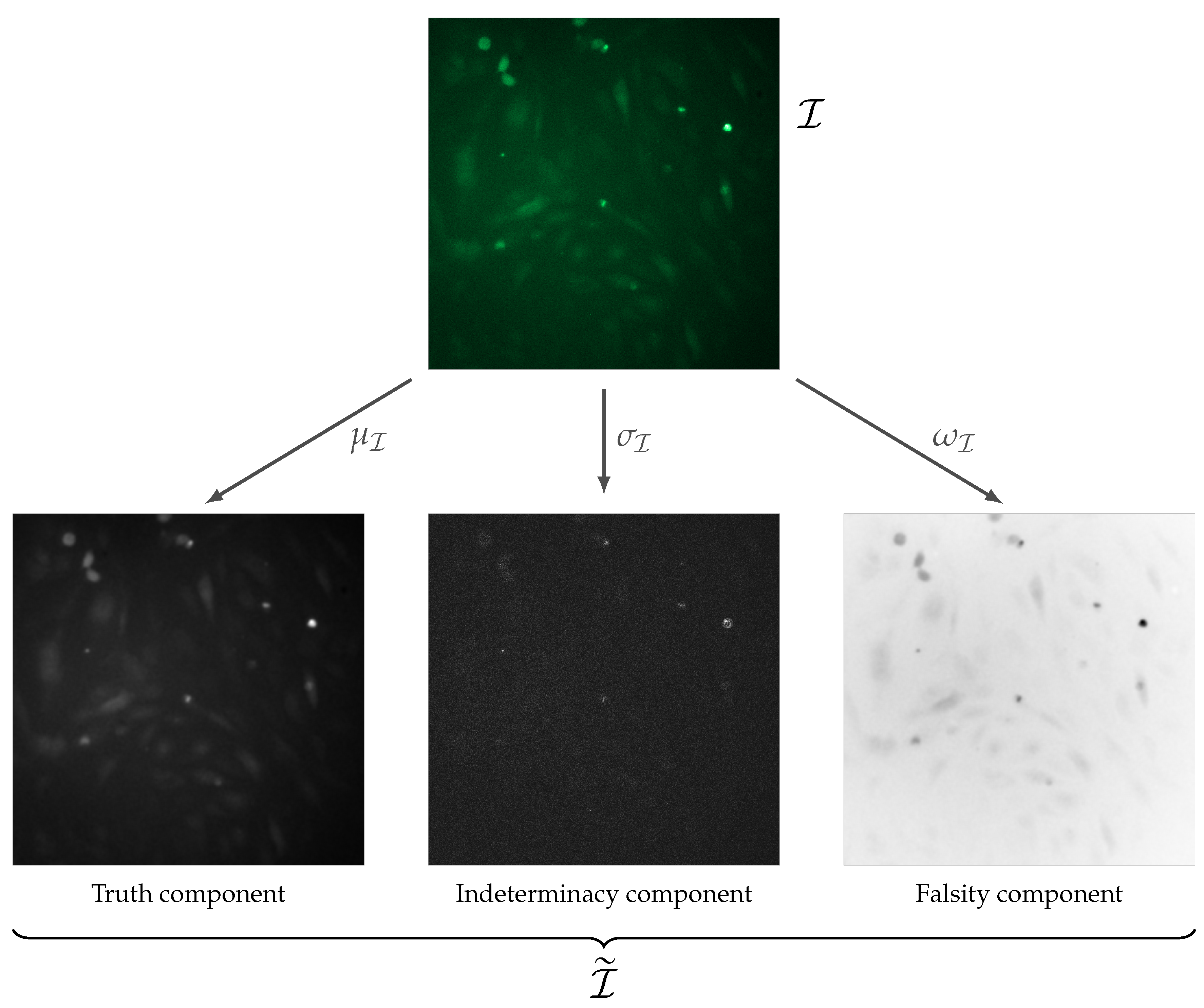
Figure 2.
Representative input fluorescence image used as reference for qualitative evaluation.
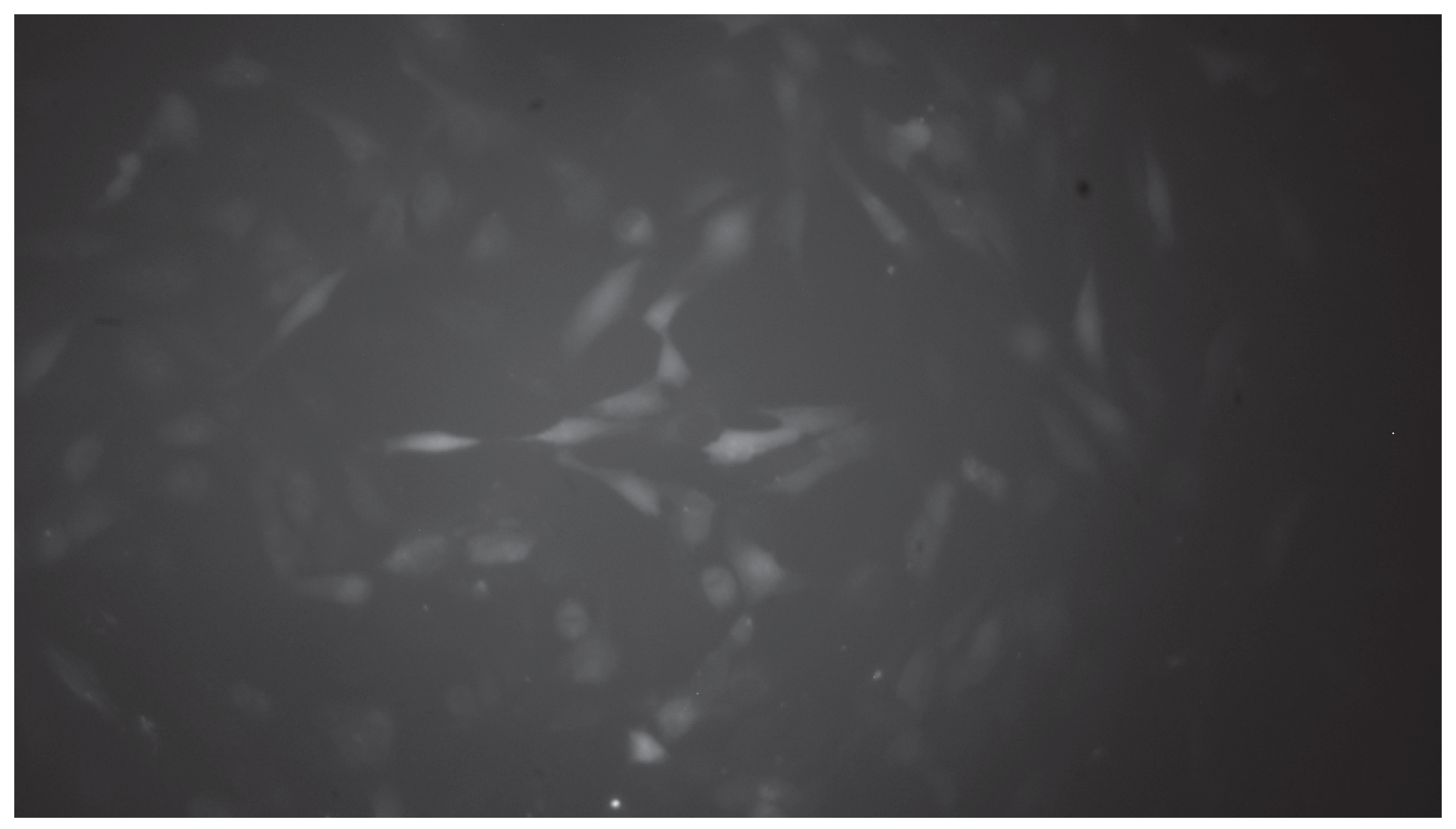
Figure 3.
Enhanced activity map corresponding to the truth component after neutrosophic morphological processing.
Figure 3.
Enhanced activity map corresponding to the truth component after neutrosophic morphological processing.
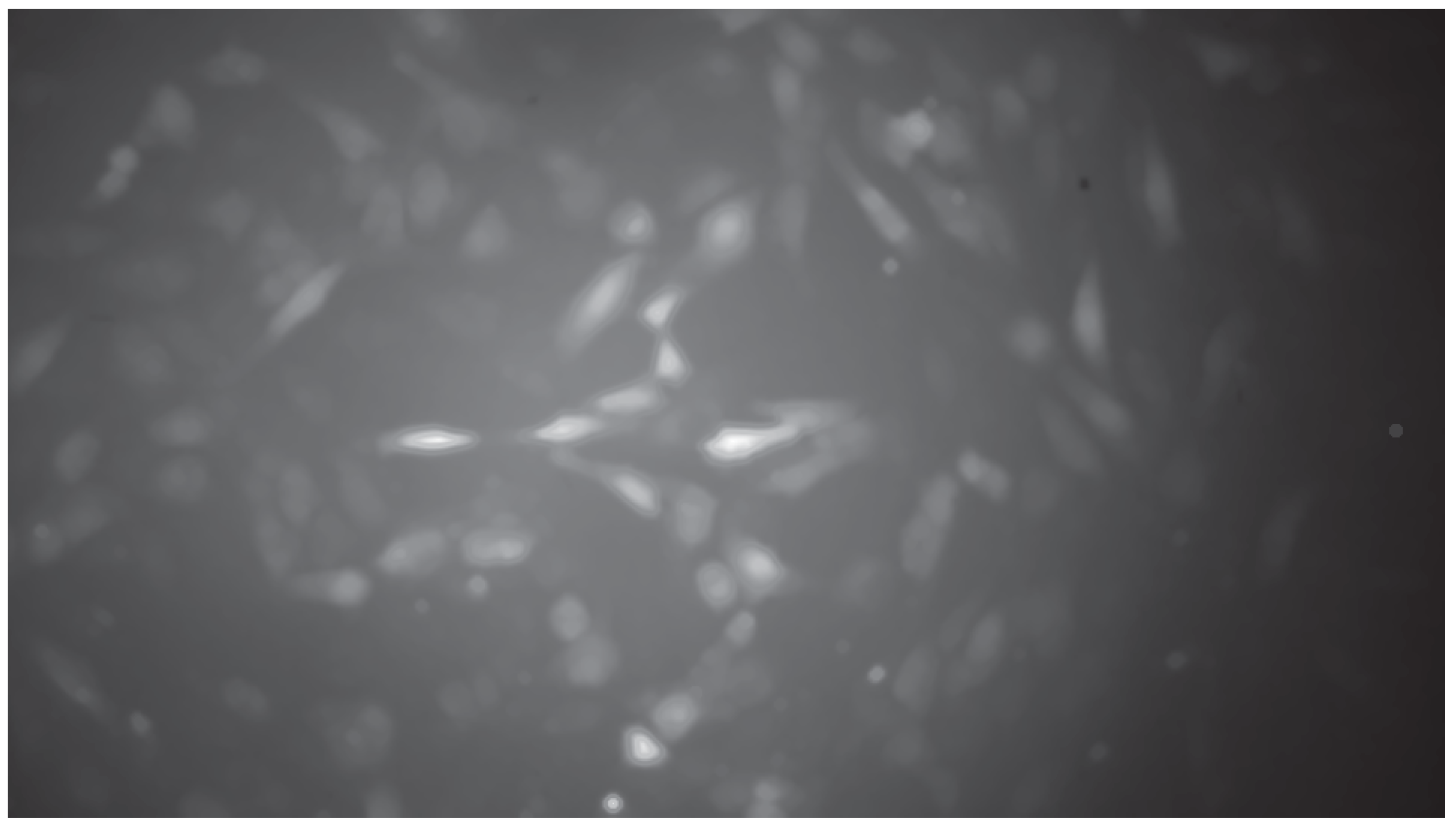
Figure 4.
Three–dimensional visualization of the enhanced truth map represented as an activity landscape. Surface height corresponds to enhanced fluorescence intensity, while circular markers indicate detected peak locations.
Figure 4.
Three–dimensional visualization of the enhanced truth map represented as an activity landscape. Surface height corresponds to enhanced fluorescence intensity, while circular markers indicate detected peak locations.
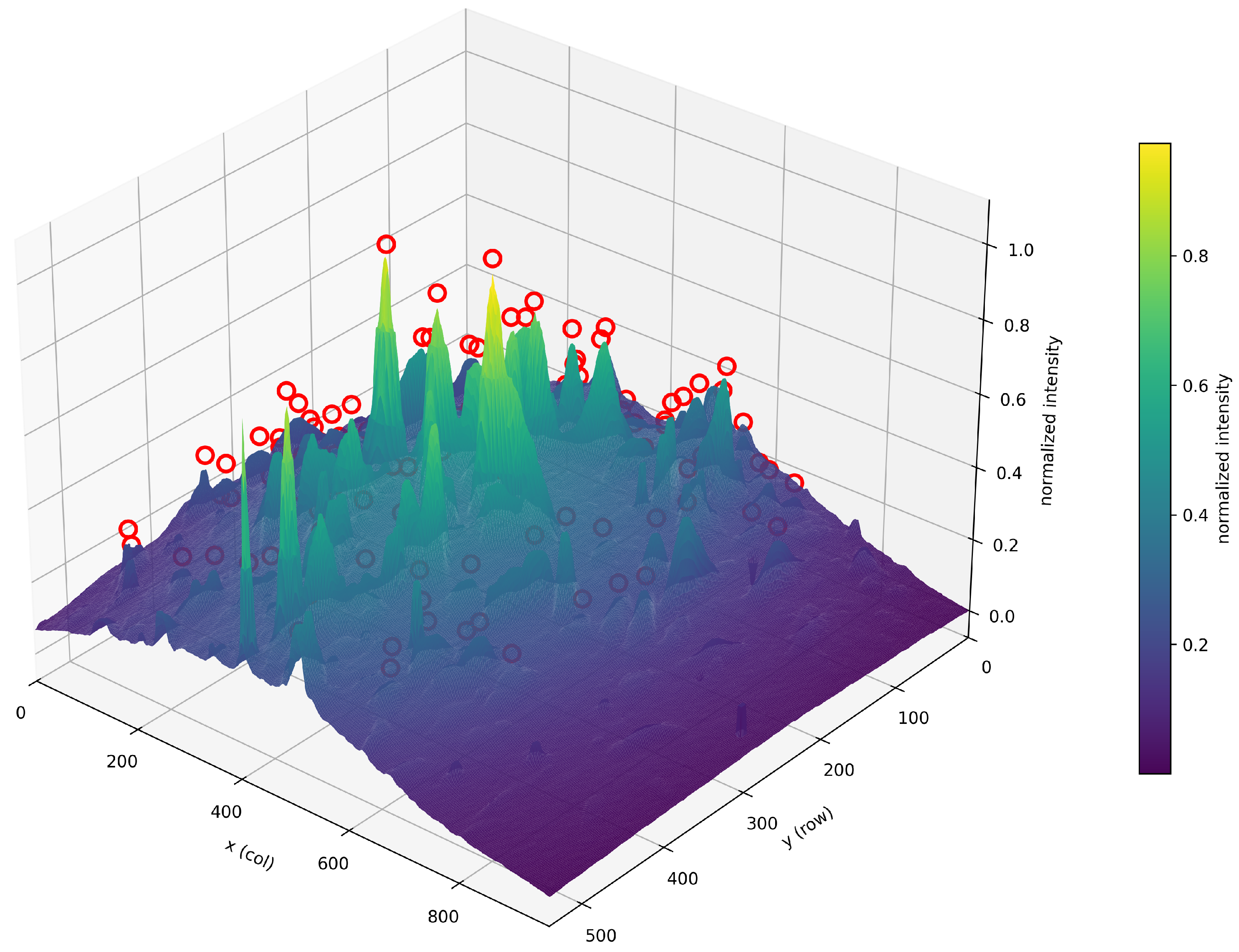
Figure 5.
Visual comparison between classical and neutrosophic peak detection results obtained on the same fluorescence time–lapse data.
Figure 5.
Visual comparison between classical and neutrosophic peak detection results obtained on the same fluorescence time–lapse data.
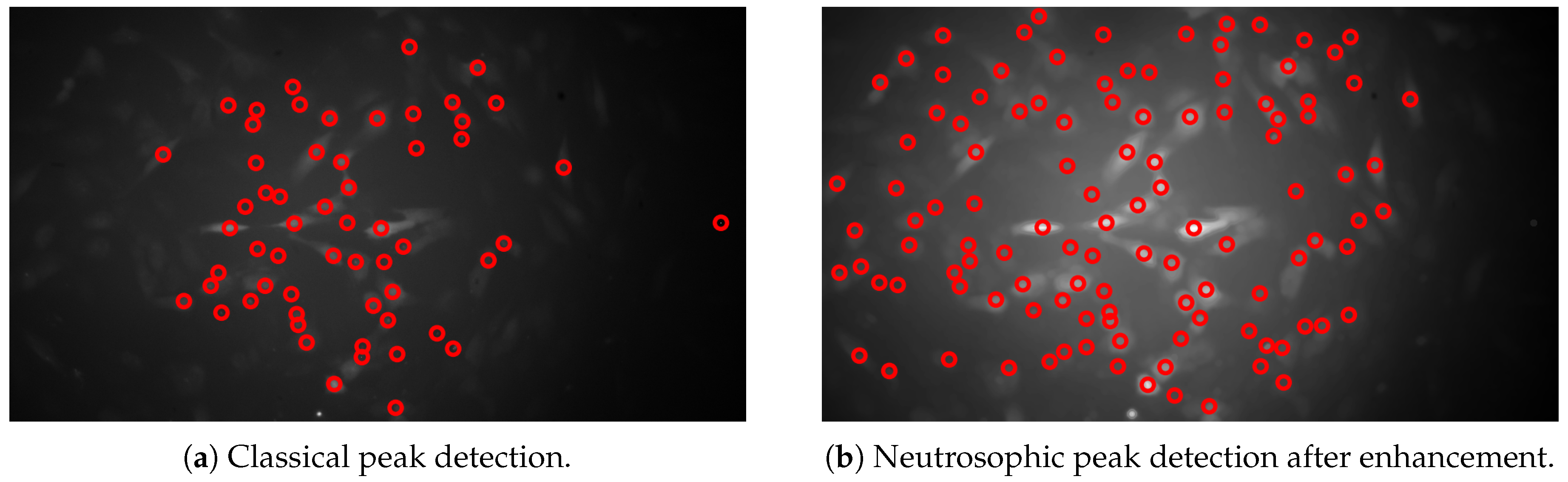
Figure 6.
Selected ROIs overlaid on the enhanced activity map. Colors correspond to the temporal traces displayed in Figure 7.
Figure 6.
Selected ROIs overlaid on the enhanced activity map. Colors correspond to the temporal traces displayed in Figure 7.
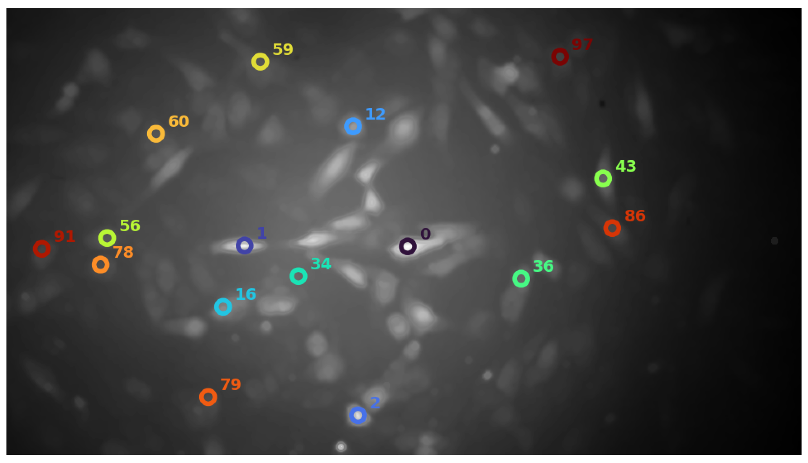
Figure 7.
Temporal fluorescence signals extracted from selected ROIs (vertically shifted for readability).
Figure 7.
Temporal fluorescence signals extracted from selected ROIs (vertically shifted for readability).
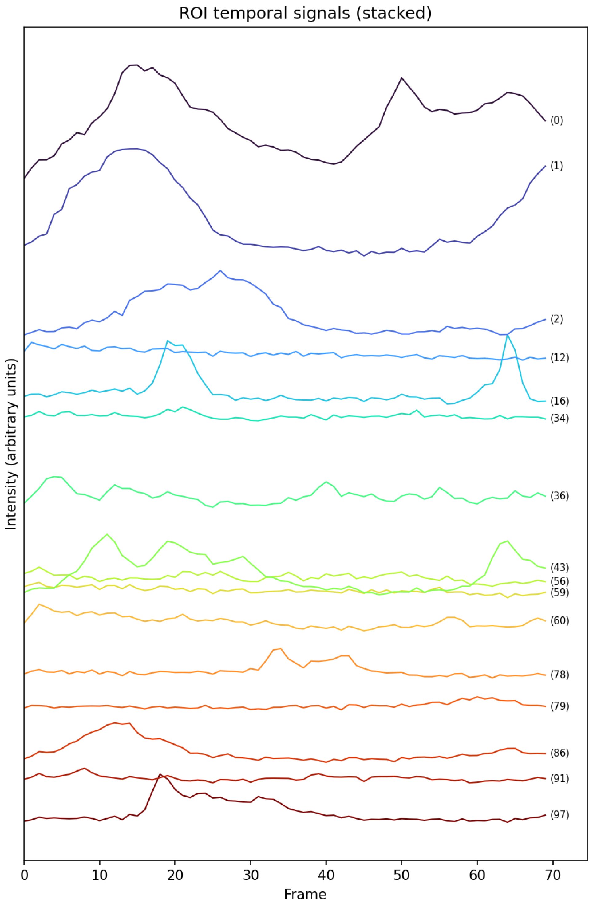
Figure 8.
Cumulative fluorescence intensity aggregated over temporal bins for each ROI.
Disclaimer/Publisher’s Note: The statements, opinions and data contained in all publications are solely those of the individual author(s) and contributor(s) and not of MDPI and/or the editor(s). MDPI and/or the editor(s) disclaim responsibility for any injury to people or property resulting from any ideas, methods, instructions or products referred to in the content. |
© 2026 by the authors. Licensee MDPI, Basel, Switzerland. This article is an open access article distributed under the terms and conditions of the Creative Commons Attribution (CC BY) license (http://creativecommons.org/licenses/by/4.0/).
Copyright: This open access article is published under a Creative Commons CC BY 4.0 license, which permit the free download, distribution, and reuse, provided that the author and preprint are cited in any reuse.