

Submitted:
24 August 2026
Posted:
25 August 2026
You are already at the latest version
Abstract
Water stress is read in the sustainability literature as either a physical or an institutional outcome, but the two readings have never been tested jointly within the sovereign ESG framework. This paper estimates the environmental, social and governance determinants of the freshwater withdrawal-to-availability ratio across up to 170 economies observed between 2002 and 2022, drawing on the World Bank Sovereign ESG Data Portal. Three equations share the same dependent variable and differ only in the pillar supplying the regressors. Each is developed along three tracks: panel econometrics, comprising pooled OLS, fixed and random effects, between and weighted least squares estimators and two-step difference and system GMM; a competition among six clustering algorithms assessed on eleven internal validity indices; and a competition among six supervised learners used to validate the specification rather than to forecast. Water stress proves overwhelmingly structural, with 99.1 per cent of its log variance lying between countries. The governance block explains 38 per cent of cross-sectional and 4 per cent of within-country variation. The level of institutional quality, measured as the first principal component of four Worldwide Governance Indicators and absorbing 91.9 per cent of their variance, is unrelated to water stress in every estimator; its composition is not, with accountability relative to state capacity carrying a coefficient of −1.10 between countries. The dominant predictor across all three tracks is the female-to-male labour force participation ratio, whose partial dependence reveals a discontinuity concentrated in a five-point interval. Under cross-validation with countries held out, no flexible learner outperforms ordinary least squares.
Keywords:
water stress
; sovereign ESG
; panel data econometrics
; institutional quality
; machine learning
1. Introduction
Water stress is the clearest case in the sustainability literature of a variable that two disciplines claim and neither concedes. Hydrology and environmental science treat the ratio of freshwater withdrawals to available renewable resources as a physical quantity, set by precipitation, geology, land cover and the sectoral composition of demand. Political science and development studies treat it as an institutional outcome, produced by allocation rules, regulatory capacity and the political settlement governing who receives water and at what price. Both readings are defensible, both are supported by substantial evidence, and they imply opposite policy conclusions: the first counsels adaptation to an endowment, the second reform of the rules governing its use. What has never been done is to test them jointly, on the same countries, with the same dependent variable and the same estimators — which is what this paper does.
The framework we use to do so is the sovereign ESG decomposition maintained by the World Bank, which sorts country-level indicators into environmental, social and governance blocks and is now embedded in sovereign debt analysis, index construction and the mandates of institutional investors. Its extension to water is not obvious, and that is precisely the point. Sovereign ESG was built to characterise the sustainability of states, not to explain physical outcomes; asking whether its three blocks explain a hydrological constraint is a test of the framework as much as of the water. If institutional quality turns out to carry little of the variation in water stress, the implication is not that governance is unimportant but that a widely used assessment architecture is silent on a resource constraint that will bind on a growing number of the sovereigns it rates.
Three gaps in the existing literature make this test possible and overdue. The first is conceptual. No study applies the sovereign ESG decomposition to water stress as a dependent variable. The only ESG-adjacent work in the field is firm-level — agribusiness corporations as water governance agents [145], corporate water stewardship [146], and the quality of corporate disclosure in high-stress jurisdictions [147] — and the term itself is effectively absent from the vocabulary of water research. The environmental, social and governance determinants of water stress are each extensively studied, in three literatures that cite one another sparsely and share almost no methodology, with the consequence that their relative explanatory weights have never been compared.
The second gap is one of estimation. The field is dominated by single-country and single-basin case studies; fewer than a dozen studies estimate determinants of water stress on cross-country data [162,163,166,168,169,170,171], and none reports the full panel apparatus that would allow within-country movement to be separated from between-country structure. The distinction is not procedural. We find that 99.1 per cent of the log variance of water stress lies between countries and 0.9 per cent within them, which means that the case-study literature and the cross-country literature have been answering different questions without saying so, and that any estimator pooling the two sources reports a coefficient dominated by the cross-section. Governance, in the same studies, enters either as a single composite or as several Worldwide Governance Indicators side by side without collinearity diagnostics — a treatment that is not innocuous, since the four dimensions prove to be close to a single latent construct.
The third gap is methodological. Machine learning appears in a bare handful of studies in this field, and never as a validation layer for an econometric specification. Non-linearities in the determinants of water stress therefore remain undetected, and the adequacy of the linear functional form is assumed rather than tested.
The paper addresses all three simultaneously. Three equations share the freshwater withdrawal-to-availability ratio as dependent variable and differ only in the pillar supplying the regressors, across up to 170 economies observed between 2002 and 2022. Each equation is developed along three tracks: panel econometrics, comprising pooled OLS, fixed and random effects, between and weighted least squares estimators and two-step difference and system GMM; a competition among six clustering algorithms assessed on eleven internal validity indices; and a competition among six supervised learners used to validate the specification rather than to forecast it.
Three results follow, and each disturbs a settled expectation. Water stress is overwhelmingly structural. The level of institutional quality — the first principal component of four governance indicators, absorbing 91.9 per cent of their variance — is unrelated to water stress in every estimator, while its composition is not: accountability relative to state capacity carries a coefficient of −1.10 between countries. And the dominant predictor across all three tracks is neither environmental nor institutional but the female-to-male labour force participation ratio, whose partial dependence reveals a discontinuity concentrated in a five-point interval, invisible to any linear specification. Under cross-validation with countries held out, no flexible learner outperforms ordinary least squares — a finding we read as evidence about the data rather than about the learners.
The article continues as follows. The second section reviews the literature pillar by pillar and states the three gaps the study addresses. The third sets out the data, the sample and the three analytical tracks applied to each equation. Sections four to six develop the environmental equation: the panel estimates, an unsupervised taxonomy of environmental regimes, and a supervised validation of the specification. Sections seven to nine repeat the sequence for the social equation, and sections ten to twelve for the governance equation, where the collinearity of the Worldwide Governance Indicators is treated as a measurement problem in all three tracks rather than as an estimation nuisance. The thirteenth section reads the nine analyses across the three pillars and identifies where they converge and where they disagree. The fourteenth draws out the implications for water policy, climate adaptation, conflict and displacement, and sovereign assessment. The fifteenth states the limitations of the design, and the sixteenth concludes.
Four appendices follow. Appendix A documents how the reviewed literature was assembled and describes its descriptive and thematic structure. Appendix B asks whether the accountability contrast recovered in the governance equation is a proxy for aridity, first by excluding the economies that anchor its lower tail and then by admitting an aridity index directly. Appendix C reports the cross-sectional dependence diagnostics, sets out why the Driscoll–Kraay covariance estimator is inappropriate in a panel of this shape, and re-estimates the two largest blocks with year fixed effects. Appendix D re-estimates the environmental and governance equations on the ninety-nine economies of the social sample, so that the ranking of the three pillars in the thirteenth section rests on a like-for-like comparison.
2. Literature Review
Water stress — the ratio of freshwater withdrawals to available renewable resources — has been studied intensively over the past fifteen years, but along three separate lines: as a physical outcome of climate and land systems, as a household and distributional condition borne disproportionately by women, and as a problem of institutions and governance. These lines correspond closely to the Environmental, Social and Governance pillars of the sovereign ESG framework, yet they are almost never brought together. They cite one another sparsely, share very little methodology, and their explanatory contributions have never been compared on a common sample of countries. The field has been reviewed before, but always from within one line or one region, so that the fragmentation is recorded rather than resolved. Existing syntheses cover Central Asia [1], groundwater governance and collective action [2], water security and trading in Australia [3], the global geography of scarcity research [4], tropical and subtropical regions [5], the evolution of scarcity indicators [6] and of potable-water security indices [7], and the behavioural and psychological literature [8]. None adopts the ESG decomposition as its organising principle, and the term itself is effectively absent from the vocabulary of the field: where it appears, it refers to corporate reporting rather than to a framework for characterising countries. The discussion is therefore organised pillar by pillar. Section 1 to 3 examine the three strands, Section 4 turns to the small quantitative literature estimating determinants on cross-country data, and Section 5 states the gaps and the contribution.
The environmental pillar. The largest and most mature strand treats water stress as a physical outcome of climate and land systems. The dominant framing is one of drylands and warming [9], mountain and glacierised regions [10], Africa under global climate change [11], and multi-regional public-health consequences [12]. Regional assessments exist for the Nile [13], for Mozambique and Zimbabwe under climate-related displacement [14], for the Yangtze River Delta under SSP–RCP scenarios [15], for India [16], for rural South Africa [17], for Islamabad [18], and for the compounding effect of the pandemic in Africa [19]. Coupled pollution and scarcity in drylands amplifies ecological degradation and social vulnerability jointly [20], which is the closest this strand comes to a cross-pillar argument. A hydrological sub-strand insists that the physical accounting itself remains incomplete: land cover change as a driver of urban water security in Kolkata [21], upwind moisture supply and moisture recycling as an invisible component of resilience [22,23], multiple-stressor interactions in aquatic ecosystems [24], managed aquifer recharge [25], and inter-basin transfers, reservoir operation and urban human–water conflict [26,27,28]. The message is that the withdrawal-to-availability ratio — the dependent variable used here — summarises a far more complex system: a limitation of the measure, not an argument against modelling it. A substantial share of the literature addresses the supply-side response without engaging determinants at all: nature-based solutions [29,30,31], constructed wetlands [32], non-conventional fluxes [33], green–grey infrastructure [34], disruptive technologies [35], desalination [36], the Kuwaiti case [37], wastewater reuse in Tunisia and Jordan [38], non-potable reuse in Sabadell [39], acceptance of greywater reuse [40], remote sensing and mobile technologies [41], ecological infrastructure investment [42], non-traditional supplies in inland communities [43], scarcity as a balancing problem [44], and general reviews of causes and mitigation [45,46,47,48]. A related literature quantifies water embodied in trade: the water footprint concept [49], intercity virtual flows in China [50], stress redistribution under consumption inequality [51], and the global drivers of local stresses in the United States [52]. This strand supplies the content of the E block almost directly, but not a comparative estimate: the evidence is case-based, and physical drivers are almost never estimated jointly with social and institutional ones.
The social pillar. The strand is organised around three concerns. The first is the food–water nexus: rural household evidence from KwaZulu-Natal [53], comparative analysis of water-stressed food systems [54], the Arab water–energy–food nexus [55], ecosystem consequences of United States policy [56], collaborative urban design [57], small-dam programmes in Ghana [58], agriculture and cattle grazing [59], water management in Algeria [60], water markets as a resilience mechanism [61], and a stochastic-control treatment of food–biodiversity outcomes [62]. The second is health: the water security–public health nexus [63], the multi-regional assessment already cited [12], and maternal health in rural Malawi [64]. The third and fastest-consolidating concern is household water insecurity as a measurable individual-level condition: a global agenda for measurement and management [65], modular and decentralised delivery [66], participatory measurement in Assam [67], household threats across settlement types in Botswana [68], behavioural and psychological research [8], water insecurity as a social rather than hydrological phenomenon [69], and who is left behind on SDG6 [70]. Justice-oriented work runs alongside: Karachi [71], irrigation efficiency gains [72], informal settlements in Kanyama [73], scarcity narratives in Brazil [74], hydro-hegemony and Global South marginalisation [75], peri-urban South Asia [76], and community systems in Mexico City [77]. Trust as a determinant of household water security [78] and a Spinozist reading of ritual water ethics in Indonesia [79] mark the interpretive edge. The gender sub-strand bears directly on the central finding of this study. Four records address it: gendered water security, rights and conflict in sub-Saharan Africa [80], water security and gender-based violence in Kenya [81], a feminist political ecology of drought in northern Nicaragua [82], and the maternal-health study cited above [64]. All four treat gender as an outcome: women bear the collection burden, the health cost and the violence risk. None treats female labour force participation as a covariate of national water stress, and the causal arrow never runs in the opposite direction or at the cross-country level. The social pillar of the sovereign framework is thus richly documented as a set of consequences and almost unexamined as a set of determinants.
The governance pillar. Governance is the most conceptually developed and least quantified pillar. Foundational work frames water security as a governance problem [83,84], sets a science agenda [85], reconciles it with integrated water resources management [86], proposes dialectical [87] and formal [88] definitions, and asks whether the concept denotes a pipe dream [89], a legal category [90], or a multilevel architecture [91]. Four directions follow. The first is adaptive and polycentric governance: adaptive management [92], institutional change under the Perth drought [93], forest landscapes [94], community governance in Ethiopia and Nepal [95], learning and civil-society action [96], science–policy networks in the arid Americas [97], the Global South [98], peri-urban Yangon [99], the Owabi catchment [100], and the political ecology of local governance in Nicaragua [101]. The second is national policy and reform: post-apartheid South Africa [102,103], Brazil [104,105,106], Pakistan [107], Jordan [108], Morocco [109,110], Kazakhstan [111], India [16], China [112,113], Malaysia [114], Chile [115], the Solomon Islands [116], small island developing states [117,118], and technological policy in Pakistan [119]. Programmatic statements on SDG6 [120] and general overviews [121] sit alongside proposals to integrate ecosystem-based with engineered governance [122], private-sector opportunity mapping [123], the water footprint of data centres [124], a data-envelopment assessment of European water security [125], and Mediterranean nature-based standards [31]. The third is transboundary and hydropolitical: a global comparative analysis of basins under climate change [126], the Nile [127], interstate conflict and cooperation [128], South Asian hydro-energy cooperation [129], the Mekong [130,131], South and Southeast Asian rivers [132], the Shenzhen River [133], delta frameworks [134], Nile adaptation [13], United States strategic engagement [135], Chinese neighbourhood diplomacy [136], Jordanian refugee and scarcity discourses [137,138], securitisation and conflict transformation [139], water theft and climate risk [140], neoliberal marginalisation [75], sovereignty in the Mekong [141], the co-evolution of water culture and security in the Weihe and Yellow basins [142,143], and participatory tools for transboundary governance [144]. The fourth is corporate and financial, and it is by far the thinnest. Agribusiness corporations as governance agents [145], water stewardship as corporate practice [146], and corporate disclosure in extremely high-stress countries [147] constitute the entire ESG-adjacent literature. All three are firm-level; none is sovereign-level, and none uses ESG as an analytical framework rather than as a description of reporting. Measurement cuts across all four: social-ecological pathway indicators [148], the water poverty index in the Koshi basin [149], headwater-to-consumer indicators [150], integrated urban assessment in the Awash basin [151] and in Palestinian cities [152], a resilience index under combined climate and conflict pressure [153], index evolution over time [7], projections to 2050 [154], and process-based basin frameworks [155,156]. A distinct urban cluster is anchored by the most cited study consulted [157] and develops through the assessment of a Global South megacity [158], a transdisciplinary synthesis [159], a global review of acute urban scarcity governance [160], and the hydro-social cycle in Catalonia [161] — the scale at which the social and governance pillars are most often studied jointly, and at which cross-country comparison is least often attempted.
The quantitative determinants literature. Fewer than fifteen studies estimate determinants of water stress on cross-country data. Vallino and colleagues relate the SDG6 integrated management indicator to crop yields and water footprints rather than to water stress directly [162]. Nkiaka examines socioeconomic determinants of water security in developing regions [163], after two indicator-based food–energy–water assessments of sub-Saharan Africa [164,165]; his finding that female primary school completion ranks among the leading determinants is the closest antecedent to our central result, though it uses schooling rather than participation and estimates a slope rather than a step. Owjimehr and co-authors estimate the effect of financial development, human development and good governance across 81 countries [166]; Munir adds economic openness and sectoral dynamics [167]. Two 2026 contributions bring governance explicitly into regression: institutional effectiveness in seventeen MENA countries [168], and technological innovation, good governance and green energy [169]. Bolognesi and colleagues relate water security to human development through size, footprint and governance, reporting non-linearities without a coefficient on any single dimension [170], extending earlier pathway measurement [148]. Ayadi reverses the direction, locating a threshold at 61.37% water stress above which sovereign borrowing costs rise sharply [171] — the only study consulted linking the hydrological variable to sovereign financial assessment. Barbier and Burgess supply the underlying theory of scarcity and efficiency [172]. Micro-econometric evidence exists for groundwater efficiency in South Indian rice farming [173] and institutional strategies in Nepalese irrigation systems [174], and a Tunisian dam study compares parametric with non-parametric classification [175]. Three features matter. The group is methodologically heterogeneous but institutionally homogeneous: quantile regression, PCSE, FGLS, threshold and smooth-transition models all appear, yet no study reports the full panel apparatus — pooled OLS, fixed and random effects, weighted least squares, between and dynamic estimators — side by side on one sample. None decomposes the variance into within- and between-country components, so it is never clear whether a coefficient describes how a country changes or how countries differ. And governance enters either as a single composite [166], as one dimension in isolation [168], or as several dimensions side by side without collinearity diagnostics [167,169]. This is not a technicality: the four Worldwide Governance Indicators are close to a single latent construct, and treating them otherwise yields estimates whose interpretation is not identified. Machine learning appears in a bare handful of studies and never as a validation layer: the Tunisian classification cited above [175], a label-noise method for naval surveillance framed as maritime water security [176], topic modelling of the tropical literature [5], and a systems-thinking review of water-security innovations [177]. No study uses supervised learning to test the stability of a panel specification, and none uses unsupervised clustering to build a taxonomy of countries by ESG-and-water profile.
Gaps and contribution. Three gaps follow, nested rather than independent. The first is conceptual: no study applies the sovereign ESG decomposition to water stress as a dependent variable, the only ESG-adjacent work being firm-level [145,146,147], so the relative explanatory contributions of the three pillars have never been compared on a common sample. The second concerns estimation: the field is dominated by single-country and single-basin case studies, and the dozen cross-country papers rarely separate within-country movement from between-country structure. That separation is decisive, since 99.1% of the variance of log water stress across 170 economies is between countries and 0.9% within them, which implies that the case-study and cross-country literatures have been answering different questions without saying so. The third is methodological: the near-absence of machine learning leaves non-linearities undetected, including the discontinuity in the female-to-male participation ratio recovered below, which engages the gender sub-strand [64,80,81,82] from the opposite causal direction and at a scale at which it has never operated. The contribution is threefold. This paper applies the sovereign ESG decomposition to water stress for the first time, estimating three equations that share one dependent variable and differ only in the pillar supplying the regressors. It reports the full panel apparatus alongside an unsupervised clustering taxonomy and a supervised machine-learning validation layer, addressing the comparative and methodological gaps simultaneously. And it treats the collinearity of the Worldwide Governance Indicators — entered side by side in [167,168] and [169] without diagnostic comment — as a substantive measurement problem, showing across all three tracks that the four dimensions represent one latent quantity whose level is unrelated to water stress and whose composition is not. None of the tracks identifies a causal effect; together they characterise the structure of the association with a completeness no single study consulted offers.
3. Data and Methodology
Data. All series are drawn from the World Bank Sovereign ESG Data Portal, which sorts country-level indicators into Environmental, Social and Governance pillars. The dependent variable throughout is the level of water stress — annual freshwater withdrawal as a proportion of available renewable resources — entered in natural logarithms. Right-skewed regressors are logged, all series are winsorised at the first and ninety-ninth percentiles, countries observed fewer than five times are dropped, and standard errors are clustered by country in every estimation. One indicator proposed for the environmental block was removed: freshwater withdrawal normalised by internal resources is a near-identical ratio to the dependent variable by construction, with a log correlation of 0.914, and its inclusion recovers an accounting identity rather than an economic relationship. It was replaced by a food production index in logs, which proxies irrigation demand and is statistically independent of the dependent variable.
Design. The ESG framework is decomposed into its three pillars and estimated as three equations that share the same dependent variable and differ only in the block supplying the regressors. The environmental equation covers 170 economies and 3,501 country-year observations between 2000 and 2021, with eight regressors spanning land use, forest cover, drought conditions, thermal exposure, population density, resource depletion and food production. The social equation covers 99 economies and 2,113 observations between 2001 and 2022, with seven regressors covering access to drinking water, sanitation and clean cooking fuel, undernourishment, fertility, labour force participation and child mortality. The governance equation covers 170 economies and 3,421 observations between 2002 and 2022, with eight regressors: four Worldwide Governance Indicators together with GDP growth, internet penetration, the female-to-male labour force participation ratio and scientific output per capita. The social sample is smaller because safely managed water and sanitation are reported for fewer countries; the environmental and governance equations are estimated on almost identical samples and are directly comparable. Each block is also estimated in the form originally proposed, retained as a robustness specification.
Each of the three equations is then developed along three tracks, applied identically across the pillars so that any difference in what they recover is a property of the block rather than of the method. The tracks answer different questions of the same data — how the association is estimated, how countries group without reference to it, and whether the functional form imposed by the estimation is adequate — and none of the three is used to identify a causal effect.
- Track 1: panel econometrics. Each equation is estimated with seven estimators — pooled OLS, fixed effects, random effects, between, weighted least squares, and two-step difference and system GMM with Windmeijer-corrected standard errors and collapsed instruments. The between and fixed-effects columns are reported side by side deliberately, since the variance of the dependent variable is decomposed into within- and between-country components before interpretation. Diagnostics comprise the F-test on individual effects, the Mundlak test in place of the classical Hausman statistic, which is degenerate under clustered covariance, the Breusch–Pagan Lagrange multiplier test, the Wooldridge autocorrelation test, the Pesaran cross-sectional dependence statistic, and Hansen and second-order serial correlation tests for the dynamic estimators. Because the four governance indicators correlate between 0.81 and 0.95, the governance block is additionally estimated in orthogonalised form, with the indicators replaced by the principal components of their standardised matrix.
- Track 2: unsupervised clustering. For each pillar the panel is collapsed to period means over the dependent variable and its regressors and standardised, yielding a country-level cross-section. Six algorithms compete — density-based, fuzzy c-means, hierarchical with Ward linkage, k-means, model-based Gaussian mixtures, and random-forest proximity clustering — each tuned on its own terms over two to eight groups. Performance is assessed on eleven internal validity indices, including silhouette, Calinski–Harabasz, Dunn, Pearson gamma, maximum diameter, minimum separation, entropy and the Herfindahl–Hirschman index of cluster concentration, aggregated into a composite rank. An admissibility rule stated in advance requires an algorithm to assign every economy to a group.
- Track 3: supervised validation. Six learners — linear regression, regression tree, k-nearest neighbours, linear support vector machine, boosting and random forest — are compared on six error and fit metrics under two schemes: a conventional random split and grouped five-fold cross-validation with entire countries held out. The selected learner is then interrogated through permutation-based dropout loss, SHAP attributions and partial dependence. The purpose is validation of functional form, not prediction.
See Figure 1.
4. Hydrological Inertia: Persistence and the Limits of Environmental Adjustment
Water stress — the ratio of freshwater withdrawal to available renewable resources — is among the least investigated dimensions of the Environmental pillar in the sovereign ESG literature, despite being the indicator most directly tied to the physical limits of national development. This first equation asks a narrow question: to what extent do environmental conditions alone account for cross-country and temporal variation in water stress, and does that association operate through the structural geography of a country or through its year-to-year climatic fluctuations?
The estimation uses the World Bank Sovereign ESG Data Portal, covering 170 economies between 2000 and 2021, for 3,501 country-year observations, of which 169 countries contribute an uninterrupted span. The dependent variable is in logs, as are the right-skewed regressors, all series are winsorised at the first and ninety-ninth percentiles, and standard errors are clustered at the country level throughout.
One indicator proposed for the block cannot enter the equation. Freshwater withdrawal normalised by internal renewable resources is, by construction, a near-identical ratio to the dependent variable, which normalises the same withdrawal by total renewable resources; the two differ only in whether inflows originating outside the national territory appear in the denominator. Their log correlation is 0.914. Estimating the specification as originally proposed returns a fixed-effects coefficient of 1.0023 on that variable with a within R² of 0.971, while the remaining seven regressors collapse to zero — agricultural land at 0.0002, forest cover at 0.0011, the drought index at 0.0001. The model recovers an accounting identity rather than an economic relationship, and the near-unit coefficient is the identity's slope.
for country i=1,…,170 and year t=2000,…,2021, where is water stress, the food production index, AGRI agricultural land, FRST forest area, SPEI the standardised precipitation–evapotranspiration index, CDD cooling degree days, LSTM mean land surface temperature, DNST population density and DRES natural resource depletion. The term is a country effect and εit an idiosyncratic disturbance clustered by country. The five static estimators differ only in the treatment of : pooled OLS sets it to zero, fixed effects removes it through the within transformation, random effects treats it as uncorrelated with the regressors, the between estimator runs on country means, and weighted least squares reweights by the inverse country-level error variance.
The dynamic columns add the lagged dependent variable,
estimated by Arellano–Bond and Blundell–Bond, two-step with Windmeijer-corrected standard errors and collapsed instruments. The social and governance equations replace xkit block by block, leaving the dependent variable and the estimator set unchanged. See Table 1.
F-test on individual effects, F(169, 3323) = 1116.83 (p < 0.001). Mundlak test χ²(8) = 42.70 (p < 0.001), favouring fixed over random effects — the classical Hausman statistic is degenerate under clustered covariance, so the Mundlak variant serves as the robust alternative. Breusch-Pagan LM = 33,794 (p < 0.001). Wooldridge AR(1) ρ = 0.8877 (p < 0.001). Pesaran CD = 23.85 (p < 0.001). For the dynamic estimators, Hansen tests return χ²(2) = 0.78 (p = 0.678) and χ²(3) = 2.12 (p = 0.548); AR(1) is rejected (p = 0.005 and 0.001) while AR(2) is not (p = 0.916 and 0.905), confirming instrument validity in both cases.
The most consequential feature of Table 1 is not any single coefficient but the gap between the between and within dimensions of the panel. The Between estimator returns an R² of 0.475; the fixed-effects specification, which discards all cross-sectional information, retains only 0.065. Roughly seven-eighths of the explanatory content of the environmental block therefore resides in permanent differences between countries rather than in movements over time. Water stress is a structural attribute of a national territory, not a variable that environmental conditions push around from one year to the next.
The Standardised Precipitation-Evapotranspiration Index makes this concrete. In the Between estimator its coefficient is −1.0447 and significant at the 1% level, one of the largest effects in the entire table; in fixed effects it is 0.0036 and indistinguishable from zero. The two estimates are not in conflict — they answer different questions. Countries that are persistently dry carry persistently high withdrawal-to-resource ratios, but a country experiencing an unusually dry year does not thereby register a measurable increase in water stress. The plausible mechanism is institutional and infrastructural rigidity: withdrawal capacity is fixed in dams, canals, irrigation networks and water rights, and none of these adjusts on an annual cycle. The same asymmetry recurs, less sharply, for forest cover and agricultural land, both strongly signed in the pooled, between and WLS columns and null once country effects absorb the cross-sectional variance.
Population density is the exception, and it is the finding worth foregrounding. Its coefficient sits between 0.33 and 0.44 across all five static estimators and is significant in every one, including fixed effects, where it survives the within transformation intact. An elasticity of roughly 0.34 means that a doubling of density is associated with about a 27% increase in water stress, holding land use, climate and resource depletion constant. Density is thus the only environmental channel in the block that generates water pressure dynamically rather than merely marking which countries are already under pressure — which makes urbanisation, not aridity, the environmental variable with genuine policy leverage.
The dynamic estimates reframe the exercise. The autoregressive coefficient of 0.8436 in difference GMM and 0.9482 in system GMM indicates that water stress is close to a unit root within countries, and this single parameter explains why almost every environmental regressor loses significance once it is included: conditional on last year's level, contemporaneous environmental conditions add essentially nothing. We read the persistence coefficient as a substantive result rather than as a nuisance parameter. It is a measure of hydrological inertia, and it is consistent with the physical account offered above — withdrawal capacity is fixed in dams, canals, irrigation networks and water rights, none of which adjusts on an annual cycle. The one variable that partially escapes is agricultural land, significant at 5% in difference GMM with a coefficient of 0.0043, small in absolute terms but surviving both differencing and instrumentation, which is a demanding standard.
Two features of the estimates deserve comment rather than silence. The first is cross-sectional dependence. The Pesaran statistic of 23.85 signals that the residuals are far from independent across countries, which is unsurprising given transboundary river basins: neighbouring economies drawing on the Nile, the Mekong or the Indus cannot have independent errors, and all are exposed to common global shocks in commodity prices and climate. Appendix C separates the two sources. Year fixed effects reduce the statistic to 3.47, so the greater part of the dependence is a common time component rather than basin sharing, and the coefficients reported above are unaffected — population density rises to 0.4572 and remains significant. The appendix also documents why the Driscoll–Kraay covariance estimator, the conventional remedy, is inappropriate in a panel of twenty-two periods and 170 economies, where it returns standard errors three to five times smaller than clustering. Basin sharing is treated here as a substantive feature of the data rather than as a nuisance to be absorbed, and what survives the year effects is the residue a transboundary reading would predict.
The second is the low within R², which is a finding rather than a shortcoming. A model that explains 47% of the cross-country variation and 6% of the variation within countries is telling us something true about the phenomenon: environmental determinants of water stress operate on geological and institutional timescales, not annual ones. That interpretation sets up the social and governance equations, where the relevant question becomes whether human and institutional variables display the same rigidity, or whether governance quality can move water stress at a horizon policy can actually reach.
5. Same Outcome, Different Mechanisms: An Environmental Taxonomy of Water Stress
The clustering unit is the country, not the country-year: the panel is collapsed to 2000–2021 period means over the nine environmental variables (the dependent variable plus the eight regressors), then standardised. This yields a cross-section of 170 countries in 9 dimensions. Each algorithm was tuned on its own terms — the partitional methods scanned over k = 2…8 with silhouette as the internal selector, DBSCAN over a grid of eps and min_samples subject to retaining at least 60% of observations, and Random Forest clustering built from a 500-tree proximity matrix against a permuted synthetic reference, then cut with average linkage. See Table 2.
Unlike the other two blocks, the algorithms do not converge here: the selected number of clusters ranges from two to seven and explained variance from 0.117 to 0.557. The environmental cross-section admits several defensible partitions rather than one, which is itself informative about its dimensionality. DBSCAN sits apart from the rest on every index, best on compactness and separation and worst on balance, with an entropy of 0.146 and a concentration index of 0.936 — the profile of a solution that discards fifty economies and places most of the remainder in a single group. Ranking the six across all eleven indices makes the trade-off explicit. See Table 3.
The rank matrix is sharply polarised rather than ordered. DBSCAN takes first place on seven indices — every separation and compactness measure, together with both information criteria — and last place on the four that reward explained variance and balanced group sizes. K-Means shows the mirror image, leading on explained variance, entropy and concentration while sitting second on almost everything else and fifth on minimum separation alone. No algorithm dominates both families, so the composite mean rank is doing real work rather than confirming an obvious winner. Figure 2 displays the same information as raw statistics, with the normalised colour scale making the two opposed patterns visible row by row. See Figure 2.
DBSCAN’s apparent dominance on the separation-type indices is an artefact worth stating explicitly, because a mechanical reading of Table 2 would select it. It achieves the best silhouette, Dunn and minimum separation only because it discards 50 of 170 countries as noise and returns a two-group solution in which one group holds 96% of the retained observations — hence entropy of 0.146 and HHI of 0.936, both worst in class. It separates cleanly by declining to classify. K-Means wins on the composite because it is the only algorithm simultaneously in the top two on explained variance, information criteria, compactness and balance, and it classifies every country. Silhouette is essentially flat between k = 3 and k = 8 (0.188–0.201), so it cannot by itself fix the number of clusters. Reading the criteria jointly, the marginal reduction in within-cluster sum of squares drops from 145 to 77 between k = 4 and k = 5 and then flattens, Davies–Bouldin reaches a plateau at 1.495, and R² attains 0.470 — the last k at which each additional cluster buys a substantial share of variance. k = 5 is therefore the selected partition; the k = 7 solution favoured by raw silhouette adds only 8 percentage points of R² at the cost of two additional groups with no distinct substantive reading. See Figure 3.
No single criterion in the figure isolates five clusters on its own. The sum of squares bends without a sharp corner, the silhouette varies by barely a hundredth across the whole range from three to eight, and the information criteria decline throughout. What supports the choice is the marginal return: the reduction in within-cluster sum of squares falls by roughly half between the fourth and fifth clusters and then flattens, and explained variance reaches 0.470 at the last point where an additional group buys a substantial share of it. The profiles that follow are where that choice has to justify itself. See Table 4.
Water stress is the back-transformed cluster mean of the log-dependent variable. SPEI is the Standardised Precipitation-Evapotranspiration Index; density is people per square kilometre; resource depletion is adjusted savings, natural resources depletion, as a share of GNI. See Figure 4.
The projection separates the clusters along two distinct axes rather than one. The first component arranges countries by thermal and hydrological regime, running from the boreal group at the left extreme to the arid group at the right, with water stress, cooling degree days and land surface temperature all loading positively and the drought index negatively. The second component is orthogonal to that gradient and is carried by forest cover against agricultural land and population density, which is what lifts the humid forested cluster clear of the two intermediate groups. Figure 5 reports the same structure variable by variable, in standard deviations from the global mean.
Membership runs as follows. C1 is the humid forest belt — Amazon (BRA, PER, COL, ECU, BOL, GUY, SUR, VEN), Congo basin (COD, COG, GAB, CMR, CAF), insular and mainland Southeast Asia (MYS, KHM, LAO, MMR, PNG). C2 is the boreal and sub-Arctic group: CAN, RUS, NOR, SWE, FIN, ISL, EST, LVA, NZL, BTN. C3, the largest, spans tropical and subtropical agrarian economies across Sub-Saharan Africa, South and Southeast Asia, Central America and the Caribbean, plus AUS, ZAF, ISR and IND. C4 is temperate Europe, East Asia and North America (DEU, FRA, ITA, ESP, GBR, USA, JPN, KOR, CHN, POL, TUR and the Balkan and Caucasus states). C5 is the arid extractive band running from the Sahel (MLI, NER, TCD, MRT) through North Africa (MAR, DZA, TUN, LBY, EGY) into the Gulf and Central Asia (SAU, ARE, KWT, QAT, BHR, OMN, IRN, IRQ, JOR, KAZ, UZB, TKM, AZE, MNG, YEM, TLS). See Table 5.
The partition orders countries almost monotonically along the water stress gradient without ever having been told to: cluster medians run 1.7%, 3.1%, 12.7%, 16.4% and 118%. This is the central validation result — the clusters were built on the joint environmental profile, and water stress separates as a by-product. See Figure 6.
The arid extractive cluster is a distinct hydrological regime rather than the tail of a continuum. Its median water stress crosses 100%, meaning that withdrawal exceeds renewable supply, sustained by fossil aquifers and desalination. Its profile is a coherent syndrome — forest cover at −1.10 standard deviations, the drought index at −1.64, resource depletion at +0.93 — that no other cluster approaches.
The tropical agrarian and temperate industrialised clusters have nearly identical water stress, at 13.0% and 14.7%, and nearly identical population density and agricultural land, but arrive there through opposite climatic routes: 3,795 cooling degree days against 335, and mean land surface temperatures of 31°C against 16°C. This is the strongest evidence in the whole exercise for why a single linear specification underperformed in the panel section. Two structurally different systems produce the same outcome, and pooling them averages the mechanisms away.
The silhouette diagnostic in Figure 5 identifies the tropical agrarian and arid extractive clusters as the weakest defined, with means of 0.127 and 0.102 and a handful of negative values in the latter. The internal heterogeneity of the arid group is real rather than a defect of the method: Gulf petro-states and Sahelian pastoral economies share aridity and resource dependence while differing in almost everything else, and the partition records that rather than resolving it.
6. Hold Out the Countries: Supervised Validation of the Environmental Specification
The target is the same as in the econometric section: the natural logarithm of water stress, regressed on the eight environmental predictors across 3,501 country-year observations and 170 economies. Six learners compete — Linear Regression, Regression Tree, K-Nearest Neighbors, Linear SVM, Boosting Decision Tree and Random Forest Regression — on MAE, MSE, RMSE, RMSLE, MAPE and R². The winning model is then used not to forecast but to interrogate the specification estimated by panel econometrics. A design decision that changes the answer Panel data with 22 observations per country and an autoregressive coefficient close to 0.9 make the standard random train-test split unsafe. Near-duplicate rows land on both sides of the partition, and the learner is rewarded for memorising country identity rather than for learning the environmental relationship. The comparison was therefore run twice: once with a conventional random 70/30 hold-out, and once with grouped five-fold cross-validation in which entire countries are held out. The gap between the two schemes is the most instructive quantity in this section. See Table 6.
Read on its own, Table 6 would settle the comparison decisively. The two ensemble methods exceed an R² of 0.95 and cut mean absolute error to roughly a quarter of the linear figure, a margin that on eight environmental indicators ought to invite suspicion rather than confidence. Each economy contributes twenty-two closely similar rows to the sample, and a random partition therefore places near-duplicates of every country on both sides of it, so a learner can score well by recognising which country a row belongs to rather than by learning how environmental conditions relate to withdrawal. Table 7 removes that possibility.
The field compresses sharply once countries are held out. Five of the six models now fall between 0.29 and 0.41, a range narrow enough that the choice among them turns on small margins, and the regression tree drops below zero — worse than predicting the sample mean. The two learners that led the random split lose most of what they appeared to have: boosting falls from 0.962 to 0.362. Random Forest Regression is the only model to finish in the upper half of both schemes, and Table 8 aggregates the two orderings across all six metrics to make that consistency explicit. See Table 8.
The composite conceals how differently the two schemes treat each model class. For the two linear learners the gap between the schemes is a matter of a few hundredths of R², while for the ensembles it exceeds half a unit and for the regression tree it spans the whole of its apparent performance. That asymmetry is the signature of leakage rather than of capability, and it is more legible in a figure than in a ranking. Figure 6 plots both schemes side by side on fit and error, and shows the out-of-fold predictions of the selected model against what was observed. See Figure 7.
Boosting reaches an R² of 0.962 under the random split and 0.362 when countries are held out. The Regression Tree falls from 0.855 to −0.025, which is worse than predicting the sample mean. Almost the entire apparent performance of the tree-based learners in Table 6 is country memorisation rather than learned structure. Random Forest Regression is selected: it wins the grouped scheme outright and is second by a narrow margin in the random one, making it the only model at the top of both. The selected model is not used for prediction. It is used to ask whether the linear panel specification captured the right variables in the right direction, through three complementary probes: dropout loss, measured as permutation importance on out-of-fold data; SHAP additive explanations; and partial dependence. Out-of-fold performance is R² = 0.480 with RMSE = 1.288, essentially the same order of magnitude as the pooled OLS R² of 0.454 reported in the econometric section. The flexible learner buys almost nothing over the linear model once countries are held out. This is itself a validation result: the linear specification is not leaving substantial structure unexploited. See Figure 8.
The ordering is dominated rather than flat. Forest cover alone accounts for more than half the baseline error and nearly twice the loss of the runner-up, and the top two variables together outweigh the remaining six. At the other end, permuting the drought index costs less than one per cent and permuting food production costs nothing measurable — the ranking that carried the largest cross-sectional coefficient in the panel section now sits second from bottom. Table 9 sets these attributions against the econometric coefficients on the same variables, where that reversal, and one genuine disagreement in sign, become visible.
The colour ordering identifies the direction of each attribution without reference to any estimator. Forest cover places its low values in the long right tail and its high values to the left; population density and land surface temperature do the reverse. Agricultural land is the exception: its colours are interleaved rather than sorted, with high values appearing on both sides of zero, which is the visual trace of a non-monotonic relationship. The bottom two variables produce almost no dispersion at all. Table 9 sets these directions against the econometric signs and records where the two methods agree, and where they do not. See Figure 9.
Seven of the eight variables agree in sign between the Between estimator and the SHAP attribution. Forest cover and population density rank first and second on every criterion — dropout loss, mean absolute SHAP and econometric significance — which is the strongest form of cross-method confirmation available in this design. See Figure 10.
Forest cover is the dominant predictor, and this was not visible in the panel section, where its fixed-effects coefficient is a non-significant −0.0042. Permuting it raises out-of-fold mean squared error by 58%, and its mean absolute SHAP value is 37% larger than that of the runner-up. The partial dependence curve in Figure 9 explains the discrepancy: the relationship is sharply non-linear, falling steeply between 0% and 35% forest cover and then flattening entirely beyond 40%. A linear coefficient averages a steep segment and a flat one into approximately zero. This is the clearest case in which the machine learning layer corrects the econometric reading rather than merely echoing it.
Population density is confirmed as the one genuinely dynamic channel. Its partial dependence is monotonic and close to linear, its SHAP direction correlation is +0.847, and its econometric coefficient survives the within transformation. Econometrics and machine learning agree completely, which is why this is the result to lead with in the policy discussion.
Agricultural land is the single disagreement, and it deserves to be reported rather than concealed. Its partial dependence is U-shaped: water stress falls as agricultural land rises to roughly 30% of territory, then rises again beyond 45%. The two arms cancel in the Between estimator, producing a negative coefficient, while the Random Forest recovers the ascending arm that dominates the upper part of the distribution. The substantive reading is that moderate agricultural extension coincides with humid, low-pressure territories, whereas extension above roughly 45% occurs in arid countries where it is irrigation-driven. A quadratic term or a spline in the panel specification would resolve the discrepancy, and testing it is a concrete robustness check the paper can offer.
A fourth observation belongs in the discussion rather than in the findings. The SPEI index collapses to near-irrelevance under grouped validation, with a dropout loss of 0.71%, despite carrying the largest coefficient in the Between estimator. This is consistent with the panel evidence: drought conditions discriminate between countries but carry no information once the model must generalise to countries it has never seen, because in the cross-section they are collinear with temperature and forest cover.
Mean absolute percentage error exceeds 190% for every model under grouped validation. This is an artefact of back-transformation to the level scale, where water stress ranges from 0.03% to 1,867%: proportional errors on the near-zero observations explode, so that misplacing a country at the bottom of the distribution by half a log point weighs more heavily than misplacing one at the top by a factor of two. MAPE is reported for completeness, since the comparative template calls for it, but it is not informative about model quality on a dependent variable spanning four orders of magnitude. Selection therefore rests on RMSE and R², both computed on the log scale.
7. Development, Not Water Policy: What the Social Pillar Explains
The environmental equation established that water stress is overwhelmingly a structural attribute of national territory: between-country variation accounted for 47% of the variance while within-country variation accounted for 6%, and the autoregressive coefficient approached unity. The natural question for the Social pillar is whether human and institutional variables display the same rigidity, or whether the social characteristics of a population can move the withdrawal-to-resource ratio at a horizon that policy can actually reach.
The dependent variable is unchanged — the natural logarithm of the level of water stress, defined as freshwater withdrawal as a proportion of available renewable resources. The regressor block is replaced entirely by Social pillar indicators covering access to services, demography, nutrition, labour and child health.
The poverty headcount at three dollars a day, proposed as one of the seven regressors, is measured through household surveys conducted at irregular intervals. It carries 2,049 observations across the period against 5,655 for under-five mortality and 6,206 for the fertility rate. Requiring it in the estimation sample reduces complete cases from 2,157 to 1,173 and, more importantly, the within-country variation that survives is largely an artefact of survey timing rather than of genuine change in poverty.
The main specification therefore replaces it with access to clean fuels and technologies for cooking, an indicator from the same Social pillar and from the Access to Services group, measured annually for 189 economies. It proxies household-level infrastructure development and correlates strongly with poverty while remaining continuously observed. The specification containing the poverty headcount as originally proposed is retained and reported in full as a robustness check, so that the reader can verify that nothing of substance turns on the substitution.
All variables enter after the same treatment used in the environmental equation: the dependent variable and the right-skewed regressors — undernourishment and under-five mortality — in logarithms, winsorisation at the first and ninety-ninth percentiles, and standard errors clustered by country throughout.
The two panels of Figure 11 invert one another. On the left, the access variables carry their weight entirely in the cross-section: the between intervals are wide and displaced from zero, while the fixed-effects intervals collapse onto it. On the right the pattern reverses for the two demographic variables, where fertility and undernourishment are precisely estimated and negative once country effects are absorbed, yet their between intervals straddle zero. Only under-five mortality retains a large positive cross-sectional coefficient with no within-country counterpart. Table 10 sets out the full estimator set behind these contrasts, together with the dynamic specifications that remove both patterns at once. See Figure 11.
The diagnostics repeat the pattern of the environmental equation. The F-test on individual effects is F(98, 2007) = 1431.37 with p below 0.001, the Mundlak test returns χ²(7) = 39.07 with p below 0.001 and therefore favours fixed over random effects, and the Breusch-Pagan Lagrange multiplier statistic is 20,760.58. The Wooldridge test yields an autoregressive parameter of 0.876, and the Pesaran cross-sectional dependence statistic is 2.816 with p = 0.005 — an order of magnitude lower than the 23.85 obtained on the environmental block, which is itself informative: social indicators are far less spatially correlated across borders than climate and land cover. See Table 11.
The single most important feature of Table 10 is a systematic reversal of sign between the Between and the fixed-effects estimators, visible at a glance in Figure 10. Sanitation coverage, clean cooking fuel access and under-five mortality all carry positive and significant coefficients in the cross-section, and all three collapse to zero once country effects are absorbed. Read naively, the Between column says that countries with better sanitation and worse child health have higher water stress — a combination that makes no causal sense.
It makes considerable descriptive sense, however. The cross-sectional coefficients are not measuring social causation but geographical confounding. The economies with the highest water stress in the sample are the arid extractive group identified by the clustering exercise: Gulf states and North African countries that combine near-universal piped sanitation and clean cooking fuel with withdrawal ratios above 100%. Their high service coverage and their high water stress are both consequences of hydrocarbon revenue and aridity, not of one another. The under-five mortality coefficient of 1.0691 in the Between estimator is driven by the opposite tail, the Sahelian countries that share the aridity without the revenue. Pooling the two into a single cross-sectional slope produces a coefficient with no interpretation.
The fixed-effects column is where the interpretable results are, and it contains exactly two. The fertility rate carries a coefficient of −0.1471, significant at the 1% level, and undernourishment carries −0.1158, significant at 5%. Both survive the within transformation, meaning they describe what happens inside a country over time rather than differences between countries. The reading is that demographic transition and improving nutrition accompany reductions in water stress, and the magnitudes are economically meaningful: a decline of one birth per woman is associated with a fall of roughly 14% in the withdrawal-to-resource ratio.
This should be interpreted as association within a development trajectory rather than as a causal effect of fertility on water use. Falling fertility, falling undernourishment and modernising irrigation infrastructure are joint features of the same transition, and the panel cannot separate them. What the coefficient does establish is that the social transition and the hydrological transition move together within countries, which is precisely what the environmental block failed to show for climate variables.
The two specifications agree on this point, which is the main purpose of reporting Table 11. In the sample restricted by the poverty headcount, fertility carries −0.2218 and undernourishment −0.2463, both at the 1% level and both larger in absolute value than in the main specification. The poverty headcount itself is never significant in any estimator. Substituting clean cooking fuel access for it costs nothing in explanatory content and nearly doubles the sample.
The dynamic estimates are, if anything, more stringent than in the environmental equation. The autoregressive coefficient is 0.738 in difference GMM and 1.004 in system GMM, and no social variable retains significance once the lagged dependent variable is included. The system GMM coefficient at unity deserves a comment in the paper rather than silence: it indicates a series that is effectively non-stationary within countries over a twenty-year window, which is consistent with water infrastructure that is built once and then persists. The difference GMM estimate of 0.738, which does not impose the level moment conditions, is the more conservative and should be the one quoted in the abstract.
The variance inflation factor on safely managed drinking water reaches 14.23 in the main specification, above the conventional threshold of ten, reflecting its collinearity with clean cooking fuel access and under-five mortality. All three are measures of the same underlying development level. The paper should either report a specification that drops drinking water coverage, or state explicitly that the block is treated as a joint development syndrome rather than as separable channels. The second option is defensible provided it is argued rather than assumed.
The sample of 99 economies is substantially smaller than the 170 available for the environmental equation, because safely managed drinking water and sanitation are reported for only 148 and 143 countries respectively. The comparison between the two equations is therefore not made on identical samples, and the economies that drop out are not a random subset: they are on average poorer or more arid, and they include the Gulf exporters that occupy the upper tail of the dependent variable. Appendix D re-estimates the environmental and governance equations on these 99 economies and finds both rankings preserved, within and between, so the comparison drawn in Section 13 is not a coverage artefact.
8. Non-Monotonic: Water Stress Along the Development Gradient
The design replicates the environmental exercise exactly. The panel is collapsed to period means over the eight social variables — the dependent variable plus the seven regressors of the main specification — and standardised, producing a cross-section of 99 economies in eight dimensions. The smaller country count relative to the environmental block reflects the limited coverage of safely managed drinking water and sanitation, reported for 148 and 143 economies respectively.
Six algorithms compete: Density-Based clustering, Fuzzy C-Means, Hierarchical clustering with Ward linkage, K-Means, Model-Based clustering with Gaussian mixtures, and Random Forest clustering built on a 600-tree proximity matrix. Each was tuned on its own terms over k = 2 to 8, with DBSCAN searched over a grid of eps and minimum sample size subject to retaining at least 60% of observations. See Table 12.
Every algorithm settles on two groups, and the five that classify all ninety-nine economies are tightly bunched: silhouettes between 0.382 and 0.465, explained variance between 0.460 and 0.520. Against them DBSCAN stands apart on almost every measure, with a silhouette of 0.649, a Dunn index of 0.728 and a separation more than double the next best — figures obtained on sixty economies rather than ninety-nine, with the retained group concentrated to the degree recorded by the entropy and concentration columns. Aggregating the eleven indices into a single ordering therefore poses a question of admissibility before it poses one of performance.

Table 13.
Rank matrix across all eleven indices (1 = best).
| Algorithm | R² | Sil. | MinSep | Dunn | Entropy | CH | Pearson | AIC | BIC | MaxDiam | HHI | Mean rank |
|---|---|---|---|---|---|---|---|---|---|---|---|---|
| Density-Based (DBSCAN) | 1 | 1 | 1 | 1 | 6 | 4 | 1 | 1 | 1 | 1 | 6 | 2.18 |
| K-Means | 2 | 3 | 3 | 3 | 4 | 1 | 2 | 2 | 2 | 3 | 4 | 2.64 |
| Fuzzy C-Means | 3 | 4 | 4 | 4 | 2.5 | 2 | 4 | 3 | 3 | 3 | 2.5 | 3.18 |
| Model-Based (GMM) | 4 | 5 | 5 | 5 | 2.5 | 3 | 5 | 4 | 4 | 3 | 2.5 | 3.91 |
| Hierarchical (Ward) | 5 | 2 | 2 | 2 | 5 | 5 | 3 | 5 | 5 | 5 | 5 | 4.00 |
| Random Forest (proximity) | 6 | 6 | 6 | 6 | 1 | 6 | 6 | 6 | 6 | 6 | 1 | 5.09 |
The polarisation observed on the environmental block returns here in a sharper form. DBSCAN now takes first place on nine of the eleven indices and last place on the two that reward balanced group sizes, entropy and concentration. The four algorithms that classify every economy are tightly bunched behind it, separated by a mean rank of 3.18 against 2.64 and by differences on the individual indices that rarely exceed one position. Random Forest proximity clustering is last on nine indices. Figure 11 shows the same matrix as raw statistics, where the near-identity of the four partitional methods is visible as an almost uniform middle band. See Figure 12.
On the social block DBSCAN does not merely perform well on the separation indices, as it did on the environmental block — it wins the composite ranking outright, with a mean rank of 2.18 against 2.64 for K-Means. The result must nonetheless be set aside, and the reason should be stated as a rule rather than improvised after the fact. DBSCAN reaches a silhouette of 0.649 and a Dunn index of 0.728 by assigning 39 of the 99 economies to noise and partitioning the remaining 60 into two groups of which one holds 88%. Its entropy of 0.393 and Herfindahl–Hirschman index of 0.769 are both the worst in the table. Eight of the eleven indices reward compactness and separation, quantities that any algorithm can improve arbitrarily by declining to classify the units that fall between groups. The composite ranking therefore has a structural bias in favour of algorithms that abstain. The purpose of this exercise is a taxonomy, and a taxonomy that leaves 39% of the sample unlabelled does not serve that purpose. The admissibility rule applied here is that an algorithm qualifies for selection only if it assigns every unit to a group. Under that rule DBSCAN is reported but excluded, and K-Means is selected — as it was on the environmental block, where it won the composite outright. Reporting the DBSCAN row rather than suppressing it allows the reader to verify that the exclusion rests on a stated criterion and not on the result.
The silhouette coefficient is maximised at k = 2, with 0.463, and declines monotonically thereafter; Davies–Bouldin is likewise minimised at k = 2. Taken alone these criteria would select a two-group partition. That partition, however, is a pure development dichotomy that carries almost no information about the dependent variable: the two groups differ in mean water stress only by 5.3% against 15.5%, and neither contains the high-stress regime as a distinct entity.
The elbow criterion points elsewhere. The marginal reduction in within-cluster sum of squares falls from 113 to 40 between k = 2 and k = 3 and then declines gently, while explained variance rises from 0.520 at k = 2 to 0.663 at k = 3 and 0.714 at k = 4. Between k = 3 and k = 5 the silhouette is effectively flat, at 0.386, 0.378 and 0.369. The partition selected is k = 4: it is the coarsest solution that isolates the high-water-stress regime as a group in its own right, and it costs 0.008 of silhouette relative to k = 3. The trade-off against the k = 2 optimum is real and is stated here rather than concealed. See Figure 13.
The three panels disagree, and the selection follows from how that disagreement is resolved. The within-cluster sum of squares bends between two and three clusters and then descends smoothly, offering no unambiguous elbow of its own. Silhouette and Calinski–Harabasz both fall monotonically from their maximum at two, so neither can select a partition on substantive grounds. The information criteria decline throughout the range without flattening. The dashed line at four marks the coarsest partition that isolates the high-water-stress regime as a group in its own right, at a cost in silhouette that Figure 13 shows to be small. Table 14 reports the resulting profiles.
Read across the rows, the first three groups form an ordered sequence: service coverage rises, fertility and child mortality fall, and water stress rises with them. The fourth group does not belong to that sequence. Its service and demographic values sit between the second and third groups on almost every column, yet its water stress is four times higher than either and its labour participation is thirteen points below the sample range of the other three. A single ordering cannot accommodate both patterns, and the projection that follows shows why: the four groups occupy two dimensions rather than one. See Figure 14.
The horizontal axis is the development gradient, running from the low-access group at the far left to the advanced-service group at the far right, with sanitation, drinking water and clean cooking fuel loading positively and fertility, undernourishment and child mortality negatively. What separates the high-stress group is vertical, not horizontal: it sits near the middle of the development axis and is pulled downward by the second component, defined by labour participation at one pole and water stress at the other. The two arrows point in almost opposite directions. The table reports the same four groups in original units, where the contrast is unmistakable. See Figure 15.
Read row by row, three of the four groups are ordered along a single gradient. The low-access group is uniformly extreme, the transitional group sits close to the global mean on every variable, and the advanced-service group mirrors the first with the signs inverted. The high-stress group breaks that ordering. Its service and demographic values are unremarkable — within a third of a standard deviation of the mean on five of the seven — while two cells stand apart: labour participation at 1.33 below and water stress at 1.04 above. The membership list that follows shows which economies produce that combination, and how heterogeneous their geography is.
Table 15.
Full cluster membership.
| Cluster | Member economies (ISO-3) |
|---|---|
| S1 · Low-access high-fertility (n = 21) | AFG, BEN, CAF, CIV, COD, ETH, GHA, GMB, GNB, MDG, MOZ, MWI, NGA, SEN, SLE, STP, TCD, TGO, TZA, UGA, ZWE |
| S2 · Transitional middle-access (n = 23) | ALB, ARM, AZE, BGD, BIH, BRA, COL, CRI, ECU, FJI, GEO, GUY, KHM, MEX, MKD, MMR, MNG, PER, PRY, SRB, SUR, TTO, VNM |
| S3 · Advanced-service (n = 41) | ARE, AUT, BEL, BLR, CAN, CHE, CHL, CYP, CZE, DEU, DNK, ESP, EST, FIN, FRA, GBR, GRC, HRV, HUN, IRL, ISR, ITA, KOR, KWT, LTU, LUX, LVA, MLT, MYS, NLD, NOR, NZL, POL, PRT, ROU, RUS, SVK, SVN, SWE, UKR, USA |
| S4 · High-stress low-participation (n = 14) | DOM, DZA, EGY, IND, IRQ, JOR, KGZ, MAR, NPL, PHL, SWZ, TUN, UZB, ZAF |
The first principal component absorbs 67.4% of total variance on its own, against 28.4% for the leading component of the environmental block. The social block is, to a first approximation, one-dimensional: drinking water, sanitation, clean cooking fuel, fertility, undernourishment and child mortality all load on a single development gradient, and knowing a country’s position on that gradient predicts the other five variables almost completely. This is a substantive finding about the structure of the Social pillar and it deserves to be stated before any discussion of individual clusters. See Figure 16.
The second component, carrying a further 14.7%, is where the interesting result lies. It is not a development axis at all: it is defined by labour force participation at one pole and water stress at the other, and it is the component that isolates cluster S4. These fourteen economies — Algeria, Egypt, Iraq, Jordan, Morocco, Tunisia and Uzbekistan alongside India, Nepal, the Philippines, the Dominican Republic, Kyrgyzstan, Eswatini and South Africa — sit at the middle of the development gradient, with service coverage close to the sample average, yet they combine labour force participation 1.33 standard deviations below the mean with water stress more than one standard deviation above it. Their median water stress is roughly 70%, against 15% in the advanced-service group. The reading is that the social syndrome associated with acute water stress is not underdevelopment. Cluster S1, the lowest-access group with fertility above five births per woman and child mortality at 85 per thousand, has the lowest water stress in the sample at 4.2%. What distinguishes S4 is an economy in which a large share of the working-age population is outside the recorded labour force and agriculture is irrigation-intensive. This gives the panel result on fertility a mechanism: within countries, the demographic transition and the labour-market transition move together, and the fixed-effects coefficient of −0.1471 on fertility is plausibly capturing that joint movement rather than fertility as such. The relationship between water stress and the development gradient is therefore non-monotonic. Water stress rises from S1 to S3 as economies develop and expand withdrawal capacity, then rises much further in S4, which is not more developed than S3 but structurally different. A linear specification on the social block cannot represent this shape, which explains why the pooled and Between estimators in the panel section returned coefficients whose signs made no causal sense.
Table 16.
Cross-tabulation of the social and environmental partitions, 98 economies in common.
| C1 Humid forested | C2 Boreal | C3 Tropical agrarian | C4 Temperate industr. | C5 Arid extractive | |
|---|---|---|---|---|---|
| S1 · Low-access high-fertility | 5 | 0 | 15 | 0 | 1 |
| S2 · Transitional middle-access | 10 | 0 | 5 | 6 | 2 |
| S3 · Advanced-service | 1 | 8 | 2 | 27 | 2 |
| S4 · High-stress low-participation | 0 | 0 | 5 | 2 | 7 |
The two taxonomies are related but not redundant. The advanced-service group S3 maps predominantly onto the temperate industrialised environmental cluster C4, with 27 of its 41 members, and the low-access group S1 maps onto the tropical agrarian cluster C3, with 15 of 21. The informative cell is S4, where 7 of 14 economies belong to the arid extractive environmental cluster C5 — but the other 7 do not. India, the Philippines, the Dominican Republic, Eswatini and South Africa reach the same high-stress social profile from a tropical agrarian environmental base, and Kyrgyzstan and Nepal from a temperate one.
This is the strongest argument the clustering section can offer for treating the Environmental and Social pillars as separate equations rather than pooling them. Aridity is one route into the high-stress regime; a labour-market and irrigation structure is another, and the two are only partially overlapping.
Cluster S2 is weakly defined, with a mean silhouette of 0.204 against 0.511 for S3, and its profile in Figure 14 is close to the global mean on every variable. It is a transitional residual rather than a type, and it is not characterised substantively here: economies that sit near the centre of the development gradient share no positive feature beyond that position, and reading a syndrome into the group would attribute content to what is in effect the space between the other three.
The overall silhouette of 0.378 is higher than the 0.193 obtained on the environmental block, which reflects the near one-dimensionality of the social data rather than a better partition. Comparisons of silhouette values across the two equations are not meaningful and should not be drawn.
9. Slow Variables, Smooth Countries: Why the Social Block Leaks
The target is unchanged — the natural logarithm of water stress — and the regressor block is the social specification estimated in the panel section: safely managed drinking water, safely managed sanitation, undernourishment, fertility, clean cooking fuel access, labour force participation and under-five mortality. Six learners compete on MAE, MSE, RMSE, RMSLE, MAPE and R². As in the environmental equation the comparison is run under two validation schemes, a conventional random 70/30 hold-out and grouped five-fold cross-validation in which entire countries are held out, so that the contribution of country memorisation can be separated from the contribution of the social variables themselves.
Taken at face value, Table 17 would be read as a decisive victory for flexible learners over linear ones. Three models exceed an R² of 0.93 while the two linear specifications sit below 0.31, and the mean absolute percentage error of the nearest-neighbour model, at 14.93, is roughly one fifteenth of the linear figure. A gap of that size on seven slow-moving social indicators should invite suspicion rather than satisfaction. Each economy contributes twenty-two closely similar rows to the sample, so a random partition places near-duplicates of every country on both sides of it. Table 18 removes that possibility by holding entire countries out.
MAE, MSE, RMSE and R² are computed on the log scale of the dependent variable; RMSLE and MAPE after back-transformation to water stress in per cent. Grouped results are averages across the five folds.
The ordering does not merely compress; it inverts. The three learners that led the random split now occupy the bottom three positions, all with negative R², meaning they predict held-out economies worse than the sample mean would. The two linear specifications, last under the random partition, move into the upper half without their own performance improving materially — the linear regression falls from 0.302 to 0.071 and the support vector machine from 0.292 to 0.116. Only Random Forest Regression finishes in the upper half of both schemes. Table 19 aggregates the two orderings across all six metrics, which is what the selection rests on.
The two shades in the left panel measure the same models on the same data and diverge by almost a full unit of R² for the tree-based learners, while barely separating for the two linear ones — the visual signature of leakage rather than of capability. The centre panel shows the consequence: under grouped validation the error bars converge to a narrow band around 1.5 log points regardless of model class. The scatter on the right makes the ceiling concrete, with predictions compressed between one and four against observations spanning zero to eight. Table 19 aggregates both schemes into the ranking on which the selection rests. See Figure 17.
KNN reaches an R² of 0.9345 under the random split and −0.1621 when countries are held out. Boosting falls from 0.9411 to −0.0750, and the Regression Tree from 0.7478 to −0.2828. Three of the six learners perform worse than predicting the sample mean once they must generalise to economies they have not seen. The reason is structural: social indicators move slowly and smoothly within countries, so a random split leaves each country represented on both sides of the partition and the learner needs only to recognise which country a row belongs to.
Random Forest Regression is selected on the composite ranking, with a mean rank of 2.00. Linear SVM ranks best in the grouped scheme alone, at 1.3, and Random Forest second at 1.8, but the SVM collapses under the random split and cannot be defended as an overall choice. The selection is consistent with the environmental equation, where Random Forest also won.
Out-of-fold performance of the selected model is R² = 0.153 with RMSE = 1.508. This is the central number of the section and it should be reported prominently rather than buried. The equivalent figure on the environmental block was 0.480. A flexible non-parametric learner, given seven social variables and free to fit any functional form or interaction, explains roughly fifteen per cent of the cross-country variation in water stress.
This is not a failure of the method; it is a finding about the Social pillar. The panel section reached the same conclusion by a different route, with a Between R² of 0.303 and a within R² of 0.109, and the clustering section reached it by a third, showing that the social block collapses onto a single development gradient that is largely orthogonal to hydrological pressure. Three independent techniques agree that social characteristics are weak predictors of water stress. The paper is stronger for saying so directly than for presenting a marginal result as a substantive one. See Figure 18.
The ordering is flat rather than dominated. No variable exceeds 28% and the seven descend in even steps, against a leading loss of 58% on the environmental block where the gap to the runner-up was itself larger than most of the bars shown here. Nothing in this block plays the role forest cover played there. The two variables that carried the fixed-effects results, fertility and undernourishment, appear fifth and seventh. Table 20 sets the ranking against the econometric coefficients and the SHAP attributions, and the comparison with the fixed-effects column is where the apparent inconsistency, and its resolution, become visible.
The colour ordering runs the same way for every variable but one. Clean cooking fuel, drinking water, sanitation and under-five mortality all place their high values to the right of zero and their low values to the left, so that better service coverage and worse child health both push predictions upward. Labour participation reverses this: its high values sit left of zero and its low values form the long right tail. The dispersions differ as much as the directions, with sanitation producing isolated contributions beyond three while undernourishment stays within a narrow band. Table 20 pairs these attributions with the econometric coefficients on the same variables. See Figure 19.
All seven variables agree in sign between the Between estimator and the SHAP attribution — a perfect concordance, against seven of eight on the environmental block. The agreement is worth reporting, but it should be read with care: it confirms that the two methods describe the same cross-sectional pattern, not that the pattern is causal. Both are recovering the same confounded association identified in the panel section, in which service coverage and water stress rise together because arid high-income economies score highly on both. See Figure 20.
Clean cooking fuel access is the leading variable by dropout loss, at 27.57%, and by mean absolute SHAP, at 0.364. Its partial dependence rises monotonically and steeply from near-zero coverage to about 55%, then flattens. Read together with the panel evidence, in which its fixed-effects coefficient is an insignificant +0.0013 while its Between coefficient is +0.0228 at the 5% level, the variable is functioning as a marker of position on the development gradient rather than as a channel. It predicts water stress because it predicts which kind of economy a country is.
Labour force participation is the second variable and the only one carrying a negative attribution, with a SHAP direction correlation of −0.682. Its partial dependence falls sharply between 45% and 60% participation and then flattens, which is precisely the discontinuity that isolated cluster S4 in the taxonomy. This is the one social variable whose importance in the machine-learning layer is not simply a restatement of the development gradient, and it is the result the paper should foreground. Its econometric coefficient is never significant in any estimator, so without the machine-learning layer it would have been discarded.
Fertility and undernourishment, the only two variables significant in fixed effects, rank fifth and seventh by dropout loss, at 7.38% and 2.98%. The inversion is instructive rather than contradictory. The panel fixed-effects estimator identifies within-country movement over time; the Random Forest, trained on a cross-section of country-years and validated across countries, identifies between-country differences. Fertility matters for how a given country’s water stress evolves and does not help in ranking countries against one another; clean fuel access does the opposite. Stating this explicitly is the cleanest way to reconcile Table 10 and Table 20 and turns an apparent inconsistency into the methodological point of the section.
The sanitation partial dependence curve is U-shaped, with elevated predictions at both very low and very high coverage. The right arm is the arid high-income group; the left arm rests on few observations, as the tick marks show, and should not be interpreted. The paper should either restrict the discussion to the right arm or note the sparse support explicitly.
MAPE again exceeds 200% for every learner under grouped validation, for the same reason as in the environmental equation: back-transformation to a level scale spanning three orders of magnitude inflates proportional errors on near-zero observations. It is reported for completeness because the comparative template requires it, but selection rests on RMSE and R².
10. Does Institutional Quality Move Water? Panel Evidence on the Governance Block
The environmental equation established that water stress is overwhelmingly a structural attribute of national territory, and the social equation established that only two variables — fertility and undernourishment — move the withdrawal-to-resource ratio inside a country over time. Both blocks left the same residual question. If neither climate nor demography explains within-country movement, does institutional quality?
The Governance pillar is where the ESG literature places its strongest priors. Sovereign ESG ratings weight governance heavily precisely because it is the dimension that policy is supposed to be able to change, and the standard reading of water scarcity in the development literature distinguishes physical scarcity from economic and institutional scarcity. The equation estimated here puts that reading under a panel test.
The dependent variable is unchanged: the natural logarithm of the level of water stress, freshwater withdrawal as a proportion of available renewable resources. The regressor block is replaced entirely by Governance pillar indicators drawn from five of the six official framework groups — Government Effectiveness, Stability and Rule of Law, Human Rights, Economic Environment, Gender and Innovation.
The Governance block proposed for this model — regulatory quality, government effectiveness, rule of law, GDP growth, research and development expenditure and the Economic and Social Rights Performance Score — cannot be estimated on a sample comparable to the environmental and social equations. Research and development expenditure carries 2,161 observations jointly with water stress and the rights score only 2,347, the latter confined to 2007–2020. Requiring both reduces complete cases to 1,144 across 95 economies, a third of the environmental sample, and truncates the period to fourteen years.
The main specification therefore substitutes within group. The Human Rights group provides Voice and Accountability in place of the rights performance score; the Innovation group provides scientific and technical journal articles, normalised per million inhabitants and logged, in place of research and development expenditure; and the block is completed with two indicators that the original proposal did not use but that belong to the same pillar and are annually observed — internet penetration from the Economic Environment group and the ratio of female to male labour force participation from the Gender group. The specification as originally proposed is retained and reported in full as a robustness check.
The second constraint is temporal rather than cross-sectional. The Worldwide Governance Indicators are published biennially from 1996 to 2002 and annually thereafter, so any panel starting in 1996 contains structural gaps in 1997, 1999 and 2001. Gaps of this kind are tolerable for static estimators but corrupt the lag structure of a dynamic panel and distort the Wooldridge autocorrelation test. The estimation window is therefore 2002–2022, twenty-one consecutive years, which yields 3,421 country-year observations on 170 economies — almost exactly the 3,501 observations and 170 economies of the environmental equation, so that the three blocks are comparable in a way the social equation was not.
Transformations follow the environmental and social equations: the dependent variable and the article count in logarithms, winsorisation at the first and ninety-ninth percentiles, standard errors clustered by country throughout, and countries retained only if observed at least five times.
The four Worldwide Governance Indicators used here correlate between 0.81 and 0.95 with one another. This is not a nuisance to be noted in a footnote; it determines what the coefficients mean. The variance inflation factors in the main specification are 17.35 on rule of law, 14.60 on government effectiveness and 11.89 on regulatory quality, all above the conventional threshold of ten, and the block behaves accordingly: coefficients are large, offsetting and unstable, and the apparent significance of individual dimensions is not robust to their joint entry.
The paper therefore reports the block three ways. First in its natural form, so that the result is comparable with the published literature that enters WGI dimensions side by side. Second under a diagnostic that enters each dimension singly, which shows what the joint specification is doing. Third in orthogonalised form, replacing the four correlated indicators with the principal components of their standardised covariance matrix. The third is the specification on which the substantive claim of the paper rests, and the choice of an explicit orthogonalisation is the methodological element that distinguishes this equation from the other two in the model.
Table 21.
Governance determinants of water stress, main specification (G-B), 2002–2022.
| Pooled OLS | Fixed Effects | Random Effects | Between | WLS | Diff-GMM | Sys-GMM | |
|---|---|---|---|---|---|---|---|
| L1.lnWS | — | — | — | — | — | 0.5782** (0.2826) | 0.9914*** (0.0147) |
| Government effectiveness | 0.0768 (0.3226) | 0.0528* (0.0308) | 0.0528* (0.0310) | −0.0123 (0.5852) | −0.8459 (0.5751) | 0.0072 (0.0126) | −0.0072 (0.0195) |
| Regulatory quality | 0.1724 (0.3432) | 0.0617 (0.0579) | 0.0606 (0.0576) | 0.1695 (0.4775) | 0.8220 (0.5206) | 0.0210 (0.0188) | 0.0055 (0.0244) |
| Rule of law | 0.6801* (0.3990) | −0.1781** (0.0843) | −0.1723** (0.0839) | 0.8811 (0.5985) | 1.7676*** (0.6717) | −0.0291 (0.0326) | 0.0073 (0.0393) |
| Voice and accountability | −0.9915*** (0.2337) | 0.0656* (0.0375) | 0.0567 (0.0374) | −1.0963*** (0.2917) | −1.3898*** (0.3750) | 0.0044 (0.0230) | −0.0067 (0.0214) |
| GDP growth % | 0.0123 (0.0104) | 0.0007 (0.0008) | 0.0008 (0.0008) | 0.0618 (0.0798) | 0.0241 (0.0179) | 0.0008 (0.0008) | 0.0011 (0.0008) |
| Internet users % | −0.0004 (0.0038) | −0.0011* (0.0007) | −0.0011* (0.0007) | −0.0007 (0.0132) | 0.0151** (0.0068) | −0.0003 (0.0005) | −0.0001 (0.0001) |
| Female/male LFP ratio | −0.0399*** (0.0052) | −0.0014 (0.0030) | −0.0026 (0.0030) | −0.0403*** (0.0057) | −0.0497*** (0.0093) | −0.0010 (0.0014) | −0.0004 (0.0007) |
| Scientific articles pc (ln) | 0.1863** (0.0844) | 0.0705*** (0.0233) | 0.0736*** (0.0230) | 0.2016* (0.1170) | −0.0059 (0.1433) | 0.0100* (0.0058) | 0.0015 (0.0079) |
| Constant | 4.4516*** (0.4615) | 2.2346*** (0.2361) | 2.2994*** (0.2625) | 4.2554*** (0.6785) | 5.3320*** (0.7468) | — | 0.0453 (0.1094) |
| N | 3,421 | 3,421 | 3,421 | 170 groups | 3,421 | 3,033 | 3,033 |
| R² | 0.3678 | 0.0410 (within) | 0.0413 | 0.3819 | 0.4890 | — | — |
Note. *** p < 0.01, ** p < 0.05, * p < 0.10. Country-clustered standard errors in parentheses. Sample: 170 economies, 3,421 country-year observations, 2002–2022. GMM estimates are two-step with Windmeijer-corrected standard errors and collapsed instruments, gmm(lnWS, 2:4), on 167 economies with at least twelve consecutive observations. Hansen tests return χ²(2) = 0.417 (p = 0.812) for difference GMM and χ²(11) = 14.539 (p = 0.205) for system GMM; AR(1) is rejected in both (p < 0.001) while AR(2) is not (p = 0.587 and 0.934).
The two panels of Figure 16 differ in what they show as much as in what they measure. On the left, the between intervals on the four institutional dimensions span two full units of the scale and all but one cross zero, while the fixed-effects intervals are so narrow as to be almost invisible at the same scale — a difference in precision of roughly an order of magnitude, and the first visible symptom of the collinearity examined below. On the right, the participation ratio and scientific output are the only variables in the block whose intervals sit clear of zero in either dimension. See Figure 21.
The variance structure of the dependent variable is the first thing to record, because it frames everything else. Across the 170 economies of this sample, 99.1% of the variance of log water stress is between countries and 0.9% is within them. The governance block explains 38.2% of the cross-sectional variation and 4.1% of the within variation — the same asymmetry found on the environmental block, where the corresponding figures were 47% and 6%, and confirmation that the pattern is a property of the dependent variable rather than of any particular set of regressors.
The diagnostics are consistent with the two preceding equations. The F-test on individual effects is F(169, 3243) = 1335.35 with p below 0.001, the Mundlak test returns χ²(8) = 95.80 with p below 0.001 and therefore favours fixed over random effects, and the Breusch-Pagan Lagrange multiplier statistic is 30,828.12. The Wooldridge autoregressive parameter is 0.871, close to the 0.876 of the social equation. The Pesaran cross-sectional dependence statistic is 5.007 with p below 0.001, between the 23.85 of the environmental block and the 2.816 of the social block: institutional quality is more spatially clustered than social indicators and less so than climate.
Table 22.
Collinearity diagnostics: each WGI dimension entered singly against joint entry.
| VIF, joint | VIF, singly | FE, singly | FE, jointly | Between, singly | Between, jointly | |
|---|---|---|---|---|---|---|
| Government effectiveness | 14.60 | 3.73 | 0.0324 (0.0317) | 0.0528* (0.0308) | 0.0585 (0.2863) | −0.0123 (0.5852) |
| Regulatory quality | 11.89 | 3.09 | 0.0191 (0.0375) | 0.0617 (0.0579) | −0.0435 (0.2592) | 0.1695 (0.4775) |
| Rule of law | 17.35 | 3.04 | −0.0641 (0.0579) | −0.1781** (0.0843) | −0.0179 (0.2145) | 0.8811 (0.5985) |
| Voice and accountability | 4.80 | 2.05 | 0.0115 (0.0390) | 0.0656* (0.0375) | −0.5230*** (0.1985) | −1.0963*** (0.2917) |
| Institutional quality (PC1) | 3.52 | 3.30 | 0.0035 (0.0280) | 0.0032 (0.0282) | −0.1247 (0.1280) | 0.0481 (0.1287) |
| Institutional balance (PC2) | 1.22 | 1.15 | −0.0096 (0.0360) | −0.0094 (0.0365) | −1.0678*** (0.3010) | −1.1044*** (0.3092) |
Note. Single entry retains the four non-WGI controls — GDP growth, internet penetration, the female-to-male labour force participation ratio and logged articles per capita — and adds one institutional variable at a time. Joint entry is the corresponding column of Table 17 for the four WGI dimensions and of Table 19 for the two principal components.
The premise of the diagnostic is visible before any coefficient is examined. The three capacity dimensions correlate at 0.94 with one another and between 0.81 and 0.88 with voice and accountability, so the block contains far less independent information than its four columns suggest. The scree plot makes the consequence explicit: one component absorbs almost everything and the remaining three share what is left. The loadings show why the first is uninformative as a contrast — all four dimensions enter it with nearly equal weight — and why the second is not, since voice and accountability alone loads positively against the three capacity measures. See Figure 22.
What that latent structure does to the estimates can be shown directly, by entering each dimension on its own and then alongside the other three. If the four measured distinct institutional attributes, the two sets of coefficients would differ only marginally. Figure 23 reports them side by side under both estimators, and the comparison is the diagnostic on which the orthogonalisation rests: the question is not whether individual coefficients are significant but whether their magnitude, sign and precision are stable across the two entries. Where they are not, the significance reported in the joint specification belongs to the specification rather than to the variable. See Figure 23.
Table 18 and Figure 23 make the same point twice. Under fixed effects, no WGI dimension is significant when entered on its own. Rule of law carries −0.0641 with a standard error of 0.0579; government effectiveness carries 0.0324 with a standard error of 0.0317. Entered jointly, rule of law becomes −0.1781 and significant at 5% while government effectiveness becomes 0.0528 and significant at 10%, and the two move in opposite directions. The pattern — coefficients inflating and splitting in sign as collinear regressors are added — is the textbook signature of variance inflation, and the honest conclusion is that the significant rule-of-law coefficient in the fixed-effects column of Table 17 is an artefact of the specification rather than a finding.
The Between estimator behaves differently, and the difference is informative. Voice and accountability is the one dimension whose cross-sectional coefficient survives single entry: −0.5230 with a standard error of 0.1985, significant at 1%. Joint entry roughly doubles it to −1.0963, which is inflation of the same kind, but the sign, the significance and the ordering are stable in a way that nothing else in the block is. The first two principal components confirm this from the other direction: they are almost unaffected by joint entry, with the second component moving from −1.0678 to −1.1044.
The four standardised WGI dimensions have a first principal component accounting for 91.9% of their variance, with loadings between 0.477 and 0.513 — an almost perfectly equal-weighted average, correlated 0.964, 0.970, 0.983 and 0.915 with government effectiveness, regulatory quality, rule of law and voice and accountability respectively. It is labelled institutional quality. The second component accounts for a further 5.6% and is a contrast: voice and accountability loads +0.848 against government effectiveness at −0.433 and regulatory quality at −0.297. It measures accountability relative to state capacity, and is labelled institutional balance. The remaining two components account for 2.5% together and are discarded.
Table 23.
Orthogonalised governance specification, principal components of the WGI block.
| Pooled OLS | Fixed Effects | Random Effects | Between | WLS | Diff-GMM | Sys-GMM | |
|---|---|---|---|---|---|---|---|
| L1.lnWS | — | — | — | — | — | 0.6616*** (0.2292) | 0.9834*** (0.0117) |
| Institutional quality (PC1) | 0.0195 (0.0924) | 0.0032 (0.0282) | 0.0011 (0.0275) | 0.0481 (0.1287) | 0.3866 (0.2460) | 0.0017 (0.0123) | 0.0008 (0.0115) |
| Institutional balance (PC2) | −0.9731*** (0.2395) | −0.0094 (0.0365) | −0.0155 (0.0367) | −1.1044*** (0.3092) | −0.8537 (0.5316) | −0.0059 (0.0226) | −0.0115 (0.0188) |
| GDP growth % | 0.0128 (0.0104) | 0.0005 (0.0008) | 0.0006 (0.0008) | 0.0565 (0.0810) | 0.0269 (0.0230) | 0.0008 (0.0009) | 0.0012* (0.0007) |
| Internet users % | −0.0017 (0.0035) | −0.0010 (0.0007) | −0.0010 (0.0007) | −0.0039 (0.0122) | 0.0085 (0.0080) | −0.0003 (0.0006) | −0.0001 (0.0003) |
| Female/male LFP ratio | −0.0396*** (0.0052) | −0.0015 (0.0030) | −0.0028 (0.0029) | −0.0397*** (0.0057) | −0.0442*** (0.0141) | −0.0010 (0.0012) | −0.0008 (0.0006) |
| Scientific articles pc (ln) | 0.1854** (0.0848) | 0.0694*** (0.0233) | 0.0725*** (0.0230) | 0.1979* (0.1159) | −0.0486 (0.2383) | 0.0104 (0.0083) | 0.0028 (0.0141) |
| Constant | 4.4655*** (0.4458) | 2.2612*** (0.2350) | 2.3266*** (0.2597) | 4.3423*** (0.6595) | 5.2529*** (1.2600) | — | 0.0867 (0.0531) |
| N | 3,421 | 3,421 | 3,421 | 170 groups | 3,421 | 3,033 | 3,033 |
| R² | 0.3614 | 0.0266 (within) | 0.0288 | 0.3745 | 0.4150 | — | — |
Note. *** p < 0.01, ** p < 0.05, * p < 0.10. Country-clustered standard errors in parentheses. Maximum variance inflation factor 4.70, on logged articles per capita; the two components carry 3.52 and 1.22. Hansen tests return χ²(2) = 0.150 (p = 0.928) for difference GMM and χ²(9) = 9.999 (p = 0.351) for system GMM; AR(2) is not rejected (p = 0.667 and 0.920).
The two components can be read directly against the data they summarise, without the intermediation of any estimator. Plotted against country means of log water stress, the level of institutional quality produces a scatter with no discernible slope, while the accountability contrast produces a clear negative one. The comparison also identifies which economies generate the second relationship, and the labels matter for the interpretation offered below: the extreme lower-left region is occupied almost entirely by Gulf hydrocarbon exporters, with one conspicuous exception whose withdrawal ratio has a different origin altogether. Figure 24 reports both scatters with the correlation coefficients.
The orthogonalised block delivers a clean and rather striking result. The level of institutional quality is unrelated to water stress in every estimator: 0.0195 in pooled OLS, 0.0032 under fixed effects, 0.0481 in the Between column, none of them within reach of significance, and a raw cross-sectional correlation of 0.091 between country means. The composition of institutional quality is strongly related to it: the second component carries −0.9731 in pooled OLS and −1.1044 in the Between column, both at the 1% level, with a cross-sectional correlation of −0.427.
Since the second component is high accountability relative to state capacity, the sign says that economies whose administrative and regulatory capacity runs well ahead of their accountability institutions are the water-stressed ones. Figure 19 identifies them: Saudi Arabia, the United Arab Emirates, Qatar, Bahrain and Oman occupy the extreme lower-left region, with mean withdrawal ratios of 925%, 1,689%, 406%, 165% and 107% respectively. At the opposite end sit Timor-Leste, São Tomé and Príncipe, Liberia, Belize, Costa Rica and Sierra Leone, all with accountability scores well above their capacity scores and withdrawal ratios in low single digits or below.
Three results deserve to be carried into the write-up, and one non-result deserves to be defended rather than hidden.
The first result is the null on institutional quality. The ESG framework and the sovereign rating industry treat the governance pillar as a summary of state quality, and the natural prior is that better-governed countries manage water better. On twenty-one years and 170 economies that prior is not supported in any estimator, in any specification, on either the level or the within transformation. This is a genuine finding rather than a failure of the data, and it is strengthened rather than weakened by the fact that the composite index is measured with near-perfect internal consistency: the four WGI dimensions load almost identically on their first component, so the null is not an artefact of an arbitrary weighting.
The second result is the accountability contrast. It is the only institutional signal in the block that survives the collinearity treatment, and it is exactly the kind of finding that the standard specification obscures, because entering four correlated indicators side by side spreads a contrast across four unstable coefficients. Read structurally, it says that the hydrological signature of the rentier state — high capacity, low voice, desalination and aquifer depletion financed by hydrocarbon revenue — is visible in the cross-section of water stress in a way that the general level of governance quality is not.
The reservation that accompanies it is the same one that governed the social equation. The economies at the bottom of the accountability contrast are also, with few exceptions, the most arid in the sample, and aridity and the political economy of hydrocarbon rents are jointly determined by geology. The Between estimator alone cannot separate them, and Appendix B does so directly: admitting a standardised aridity index attenuates the coefficient by under four per cent, and excluding the Gulf economies leaves it significant at five per cent. The contrast is therefore not a rainfall regime in disguise. It remains, however, a descriptive regularity of the cross-section rather than an identified effect, and the counter-examples are instructive. Singapore sits at the extreme low end of the second component with a withdrawal ratio of 192% that has nothing to do with hydrocarbon rents and everything to do with a city-state's renewable freshwater endowment, while Brunei and Malaysia sit at the same end with ratios of 3.5% and 3.2%.
The third result is the coefficient on scientific output, which is the only variable in the entire block to survive the within transformation with a stable sign. It carries 0.0705 under fixed effects, significant at 1%, and 0.0694 in the orthogonalised specification, and it retains marginal significance in difference GMM at 0.0100. A country that doubles its per-capita scientific output is associated with roughly a 5% increase in its withdrawal-to-resource ratio. The interpretation is not that research causes water stress; it is that scientific output is the best available annual proxy in this dataset for the industrial and agricultural intensification that drives withdrawal, and it is picking up the development trajectory that fertility and undernourishment picked up in the social equation, with the opposite sign because it moves in the opposite direction over the same transition.
The non-result to defend is the dynamic panel. The autoregressive coefficient is 0.578 in difference GMM and 0.991 in system GMM, and no governance variable retains significance once the lagged dependent variable enters. The system estimate at unity repeats what the social equation found and carries the same reading: within a twenty-one-year window, water stress is effectively a non-stationary series at the country level, because the infrastructure that determines it is built once and then persists. The difference GMM estimate of 0.578 is the more conservative and is the one to quote. Both pass Hansen comfortably and neither shows second-order serial correlation, so the instrument set is not the problem. What the dynamic results establish is a boundary condition on the whole model: governance indicators have no measurable short-run effect on the withdrawal ratio conditional on its own past, and any policy claim from this equation has to be a cross-sectional and structural claim rather than a dynamic one.
Table 24.
Robustness: specification as originally proposed (G-A), with R&D expenditure and the rights performance score.
Table 24.
Robustness: specification as originally proposed (G-A), with R&D expenditure and the rights performance score.
| Pooled OLS | Fixed Effects | Random Effects | Between | WLS | |
|---|---|---|---|---|---|
| Government effectiveness | 0.6377 (0.4796) | −0.1048* (0.0631) | −0.1063* (0.0628) | 1.2858 (0.7934) | −0.1101 (0.9435) |
| Regulatory quality | −0.2008 (0.4890) | 0.1125 (0.0785) | 0.1131 (0.0780) | −0.3923 (0.6106) | 0.0940 (0.6901) |
| Rule of law | −0.9300 (0.5812) | −0.2630** (0.1162) | −0.2639** (0.1107) | −1.2505 (0.7938) | −0.3684 (0.9437) |
| GDP growth % | 0.0300** (0.0126) | −0.0004 (0.0023) | −0.0002 (0.0023) | 0.0819 (0.0697) | 0.0232 (0.0165) |
| R&D expenditure % GDP | 0.1390 (0.1876) | −0.0120 (0.0531) | −0.0087 (0.0517) | 0.0436 (0.2239) | −0.0055 (0.2604) |
| Economic & social rights | 0.5118*** (0.1796) | 0.0629 (0.0783) | 0.0772 (0.0750) | 0.4814*** (0.1756) | 0.7088*** (0.2595) |
| Constant | 0.5249 (0.7068) | 2.6440*** (0.3503) | 2.5708*** (0.3469) | 0.5272 (0.7617) | 0.0954 (0.9267) |
| N | 1,144 | 1,144 | 1,144 | 95 groups | 1,144 |
| R² | 0.1487 | 0.0436 (within) | 0.0491 | 0.1794 | 0.1668 |
Note. *** p < 0.01, ** p < 0.05, * p < 0.10. Country-clustered standard errors in parentheses. Sample: 95 economies, 1,144 country-year observations, 2007–2020. The smaller sample and shorter window reflect the coverage of research and development expenditure and of the Economic and Social Rights Performance Score.
The restricted specification agrees with the main one on everything that matters and disagrees on nothing. Research and development expenditure is insignificant in all five estimators, which retrospectively justifies the substitution. The rights performance score carries 0.5118 in pooled OLS, 0.4814 in the Between column and 0.7088 under WLS, all at the 1% level, and collapses to an insignificant 0.0629 under fixed effects — a purely cross-sectional signal of the same family as the accountability contrast, though with the opposite sign, since the rights score rewards outcome achievement conditional on resources and therefore tracks development level rather than accountability. Rule of law again reaches significance under fixed effects only in joint entry with the other WGI dimensions, at −0.2630, reproducing the collinearity artefact identified in Table 18 on a completely different sample and period. That the artefact replicates is itself a small piece of evidence that the diagnostic in Table 18 is diagnosing something real.
The Pesaran statistic on this restricted sample is −0.325 with p = 0.746, against 5.007 on the main sample. The difference is a consequence of the shorter window rather than of the specification, and should not be reported as a substantive result.
The comparison across the three equations is now available on samples that are almost identical for two of the blocks — 3,501 observations and 170 economies for the environmental block, 3,421 and 170 for the governance block — against 2,113 and 99 for the social block. The within-R² ranking is environmental 0.06, governance 0.04, social 0.11, and the between-R² ranking is environmental 0.47, governance 0.38, social 0.30. The social block explains the most within-country movement and the least between-country variation; the environmental block does the reverse; governance sits between them on both. Appendix D re-estimates the environmental and governance equations on the ninety-nine economies of the social sample and finds both orderings preserved, so the ranking is not an artefact of who is in each panel. It is a result in its own right, and Section 13 develops it.
The Gulf economies drive a large share of the cross-sectional identification in this equation, as they did in the clustering exercise, and the accountability contrast could in principle be a proxy for the aridity that characterises them. Appendix B addresses this on both fronts. Excluding the six Gulf Cooperation Council members attenuates the Between coefficient on institutional balance from −1.10 to −0.83, and a wider exclusion of twenty Middle Eastern and North African economies to −0.73, both remaining significant at five per cent. Admitting a standardised aridity index directly — itself strongly and positively associated with water stress — attenuates it by under four per cent, and the interaction between the two is insignificant. The contrast is therefore not a rainfall regime in disguise, and the attenuation under exclusion reflects the loss of the range that identifies the coefficient rather than the removal of a confound.
Finally, the orthogonalisation should be presented as a deliberate design choice rather than as a repair. The literature that enters WGI dimensions jointly is large, and a paper that reports both forms — the conventional one for comparability, the orthogonalised one for inference — and shows in a single figure why they differ is making a contribution to how the governance pillar is handled empirically, not merely reporting a diagnostic.
11. Orthogonal Gradients: Institutional Quality and the Hydrological Outcome
The design replicates the environmental and social exercises exactly. The panel is collapsed to period means over the nine governance variables — the dependent variable plus the eight regressors of the main specification — and standardised, producing a cross-section of 170 economies in nine dimensions. The country count matches the environmental block and exceeds the social block by seventy-one economies, because the Worldwide Governance Indicators and the Economic Environment group are reported almost universally while safely managed drinking water and sanitation are not.
Six algorithms compete: Density-Based clustering, Fuzzy C-Means, Hierarchical clustering with Ward linkage, K-Means, Model-Based clustering with Gaussian mixtures, and Random Forest clustering built on a 600-tree proximity matrix. Each was tuned on its own terms over k = 2 to 8, with DBSCAN searched over a grid of eps and minimum sample size subject to retaining at least 60% of observations.
Table 25.
Internal validation indices, six algorithms at their own optimal configuration.
| Algorithm | k | n | R² | AIC | BIC | Sil. | MaxD | MinS | Pear. | Dunn | Ent. | CH | HHI |
|---|---|---|---|---|---|---|---|---|---|---|---|---|---|
| Density-Based (DBSCAN) | 2 | 102 | 0.322 | 2111.9 | 2161.8 | 0.268 | 7.475 | 0.959 | 0.349 | 0.128 | 0.546 | 47.39 | 0.640 |
| Fuzzy C-Means | 2 | 170 | 0.444 | 3482.3 | 3541.9 | 0.373 | 7.206 | 1.038 | 0.580 | 0.144 | 0.653 | 134.07 | 0.540 |
| Hierarchical (Ward) | 2 | 170 | 0.358 | 3701.9 | 3761.5 | 0.359 | 8.017 | 0.941 | 0.531 | 0.117 | 0.466 | 93.68 | 0.709 |
| K-Means | 2 | 170 | 0.444 | 3480.5 | 3540.1 | 0.376 | 7.206 | 0.906 | 0.586 | 0.126 | 0.646 | 134.42 | 0.547 |
| Model-Based (GMM) | 2 | 170 | 0.428 | 3524.8 | 3584.3 | 0.360 | 7.304 | 0.964 | 0.565 | 0.132 | 0.649 | 125.80 | 0.543 |
| Random Forest (proximity) | 2 | 170 | 0.427 | 3527.5 | 3587.0 | 0.347 | 7.304 | 1.100 | 0.550 | 0.151 | 0.683 | 125.29 | 0.510 |
Note. n = economies classified; Sil. = silhouette; MaxD = maximum within-cluster diameter; MinS = minimum between-cluster separation; Pear. = Pearson gamma; Ent. = entropy of cluster sizes; CH = Calinski–Harabasz; HHI = Herfindahl–Hirschman index of cluster size concentration. Higher is better for R², Sil., MinS, Pear., Dunn, Ent. and CH; lower is better for AIC, BIC, MaxD and HHI.
The governance cross-section behaves unlike the other two blocks. Every algorithm converges on two groups, and five of the six return silhouettes between 0.347 and 0.376 with explained variance between 0.358 and 0.444 — a spread too narrow for any method to be said to find structure the others miss. DBSCAN no longer dominates the separation indices: it classifies 102 of the 170 economies and still records the lowest silhouette in the table, which suggests the units it discards do not lie between well-defined groups. The ranking that follows therefore turns on small differences, and its ordering should be read accordingly.
Table 26.
Rank matrix across all eleven indices (1 = best).
| Algorithm | R² | Sil. | MinSep | Dunn | Entropy | CH | Pearson | AIC | BIC | MaxDiam | HHI | Mean rank |
|---|---|---|---|---|---|---|---|---|---|---|---|---|
| Fuzzy C-Means | 2 | 2 | 2 | 2 | 2 | 2 | 2 | 3 | 3 | 1.5 | 2 | 2.14 |
| K-Means | 1 | 1 | 6 | 5 | 4 | 1 | 1 | 2 | 2 | 1.5 | 4 | 2.59 |
| Random Forest (proximity) | 4 | 5 | 1 | 1 | 1 | 4 | 4 | 5 | 5 | 3.5 | 1 | 3.14 |
| Model-Based (GMM) | 3 | 3 | 3 | 3 | 3 | 3 | 3 | 4 | 4 | 3.5 | 3 | 3.23 |
| Density-Based (DBSCAN) | 6 | 6 | 4 | 4 | 5 | 6 | 6 | 1 | 1 | 5 | 5 | 4.45 |
| Hierarchical (Ward) |
5 | 4 | 5 | 6 | 6 | 5 | 5 | 6 | 6 | 6 | 6 | 5.45 |
The ranking rewards consistency rather than peak performance. Fuzzy C-Means never places first on any index and never below third on any of the eleven, which is enough to take the composite. K-Means leads on explained variance, silhouette, Calinski–Harabasz and Pearson gamma but falls to sixth on minimum separation and fifth on Dunn, and that pair of reversals costs it the aggregate by less than half a rank. Random Forest proximity clustering shows the opposite profile, first on the three indices where K-Means is weakest. Figure 25 displays the underlying statistics, where the near-uniform bands make the closeness of the field apparent.
The first is that the admissibility rule invoked on the social block does not bind here, because DBSCAN does not win. On the environmental and social blocks the density-based algorithm dominated the separation indices by abstaining from classification; on the governance block it abstains just as heavily — 68 of the 170 economies are assigned to noise — and still finishes fifth, with a silhouette of 0.268 against 0.376 for K-Means and the worst rank on seven of the eleven indices. The reason is substantive rather than technical. Density-based clustering finds regions of high point concentration separated by sparse regions, and the governance cross-section contains none: institutional quality is distributed as a continuum, not as a set of well-separated modes. That DBSCAN cannot buy compactness by abstaining, when it could do so on both other blocks, is itself a description of the data.
The second is the extraordinary convergence of the remaining algorithms. The adjusted Rand index between K-Means and Fuzzy C-Means at their common optimum is 0.953, between K-Means and the Gaussian mixture 0.840, and between Fuzzy C-Means and Random Forest proximity clustering 0.736. Four algorithms with entirely different objective functions recover the same two-group partition. Only Ward linkage dissents, at 0.409 against K-Means, and its partition is the worst on eight of eleven indices.
Fuzzy C-Means is selected. It takes the composite ranking with a mean rank of 2.14 against 2.59 for K-Means, and it does so without any abstention, so no admissibility question arises. The margin is narrow, and it should be read as such: K-Means wins explained variance, silhouette, Calinski–Harabasz and Pearson gamma outright, and loses the composite only on the separation and concentration indices. The selection is nonetheless the right one for a second and more substantive reason. The fuzzy memberships carry information that a hard partition destroys, and on this block that information concerns precisely the economies the equation is about.
The panel section established that the four Worldwide Governance Indicators correlate between 0.81 and 0.95 and effectively measure a single latent quantity. That fact does not disappear when the block is clustered; it changes the metric. Euclidean distance over the standardised nine-dimensional space gives each variable equal weight, so a latent dimension represented by four near-identical indicators enters the distance calculation with four times the weight of internet penetration or of the female-to-male labour force participation ratio. The first principal component of the cross-section absorbs 61.6% of total variance and is, with loadings of 0.412, 0.410, 0.411 and 0.376, an almost pure institutional-quality axis.
A robustness partition was therefore estimated on the orthogonalised block — water stress, the two retained principal components of the WGI matrix, GDP growth, internet penetration, the participation ratio and logged articles per capita, seven dimensions in which institutional quality is represented once rather than four times. The adjusted Rand index between the two partitions is 0.634: substantially related, not identical. Where they disagree is reported with the taxonomy below, and the disagreement is informative rather than embarrassing.
The silhouette coefficient is maximised at k = 2, with 0.373, and declines to 0.268 at k = 3 and 0.255 at k = 4; Davies–Bouldin is likewise minimised at k = 2. Taken alone these criteria would select a two-group partition, exactly as on the social block.
That partition is again uninformative about the dependent variable. At k = 2 the two groups differ in median water stress by 16.6% against 8.3%, and the higher-stress group is simply the richer one. At k = 3 a high-stress group begins to emerge, with a median of 26.2% and a participation ratio of 57.9, but it holds 67 of the 170 economies and mixes the regime with its neighbours. At k = 4 the group separates cleanly: 40 economies, median water stress 46.1%, participation ratio 46.4. The elbow criterion supports the same choice — the marginal reduction in within-cluster sum of squares falls from 169 to 96 between k = 3 and k = 4 and then to 53 — while explained variance rises from 0.444 at k = 2 to 0.555 at k = 3 and 0.618 at k = 4.
The partition selected is k = 4, at a cost of 0.118 of silhouette relative to the k = 2 optimum. The trade-off is larger than the 0.008 paid on the social block and should be stated plainly rather than concealed: the governance cross-section has no strong natural partition at any k, and the four-group solution is chosen because it isolates the regime the equation is about, not because the data insist on it. See Figure 26.
None of the four panels endorses the selection on its own. The sum of squares bends at three rather than four and descends smoothly thereafter, the silhouette falls monotonically from its maximum at two, explained variance rises steadily without flattening, and the partition coefficient declines throughout, from 0.706 to 0.433 at the dashed line — the solution grows fuzzier at every step. The case for four clusters rests entirely on what the additional group contains rather than on any internal criterion, and the profiles that follow are therefore the justification rather than an illustration of it. Their fourth row is where the argument stands or falls.
Table 27.
Cluster profiles, original units (period means 2002–2022).
| Cluster | n | Water stress % | Gov. eff. | Reg. quality | Rule of law | Voice | GDP growth % | Internet % | Female/male LFP | Articles per m. |
|---|---|---|---|---|---|---|---|---|---|---|
| G1 · Low-capacity agrarian | 48 | 3.28 | −0.92 | −0.88 | −0.91 | −0.76 | 4.61 | 12.7 | 83.8 | 5.2 |
| G2 · Constrained-participation | 40 | 35.40 | −0.53 | −0.57 | −0.76 | −0.77 | 4.02 | 29.0 | 46.4 | 22.9 |
| G3 · Intermediate / rentier-mixed | 42 | 10.80 | 0.09 | 0.15 | −0.03 | 0.03 | 3.30 | 47.6 | 70.2 | 105.1 |
| G4 · High-capacity democratic | 40 | 14.06 | 1.31 | 1.31 | 1.25 | 1.23 | 2.31 | 72.2 | 78.9 | 974.3 |
Note. Water stress and articles per million inhabitants are back-transformed cluster means of the corresponding logged variables; the WGI dimensions run from approximately −2.5 to +2.5. Cluster median water stress is 3.9%, 46.1%, 7.6% and 16.7% respectively.
The geometry behind these profiles separates the two things the table reports jointly. All four governance dimensions point in the same direction, to the right, together with connectivity and scientific output: this is the horizontal axis, and it orders the four groups from the low-capacity agrarian cluster to the high-capacity democratic one. Water stress and the participation ratio point almost straight up and straight down, orthogonal to that ordering, and it is this vertical axis alone that lifts the constrained-participation cluster clear of the other three. Growth is the only variable with no appreciable length in either direction. See Figure 27.
The ellipses overlap substantially in the projection, and reading group membership from position alone would be unreliable for the economies near the origin. Expressing each group as a vector of standardised means removes that ambiguity and makes the profiles directly comparable variable by variable. It also brings out what the projection compresses into two dimensions: the intermediate cluster is not merely centrally located but flat, sitting within a fifth of a standard deviation of the global mean on almost every dimension, while the constrained-participation cluster is unremarkable on the four institutional measures and extreme on exactly two. Figure 28 reports the full matrix.
The first principal component absorbs 61.6% of total variance and is the institutional-quality axis. Water stress loads on it at 0.063 — essentially zero. The governance gradient and the hydrological outcome are orthogonal in the cross-section, which is the clustering counterpart of the panel result that the first principal component of the WGI block carries a coefficient of 0.0032 under fixed effects and 0.0481 in the Between estimator, neither remotely significant.
The second component, carrying a further 17.4%, is where the structure lies. It is defined by water stress at one pole, loading 0.688, and the female-to-male labour force participation ratio at the other, loading −0.675, with every other variable below 0.20 in absolute value. It is a two-variable axis, and it is the component that isolates cluster G2.
This is a replication, from a disjoint variable set, of the finding reported on the social block. There the second component was defined by labour force participation against water stress and isolated cluster S4. Here the same contrast reappears among governance indicators — the participation ratio belongs to the Gender group of the Governance pillar, the labour force participation rate to the Social pillar — and isolates a group of forty economies rather than fourteen. Two independent blocks of the ESG framework, sharing no variable other than the dependent one, locate the high-water-stress regime along the same axis.
Cluster G1, forty-eight economies, is the worst-governed group in the sample: government effectiveness at −0.92, internet penetration at 12.7%, five scientific articles per million inhabitants. It also has the lowest water stress in the sample, a geometric mean of 3.3% and a median of 3.9%, and the highest female-to-male participation ratio at 83.8. It is predominantly Sub-Saharan African, with Cambodia, Laos, Myanmar, Mongolia, Papua New Guinea, Timor-Leste, Viet Nam, Bolivia and Paraguay attached.
Cluster G2, forty economies, is the object of the exercise. Its governance scores are below average but not extreme — government effectiveness at −0.53, better than G1 on every WGI dimension — while its water stress is an order of magnitude higher, a geometric mean of 35.4% and a median of 46.1%. Its distinguishing feature is not institutional at all: a female-to-male labour force participation ratio of 46.4, fully 1.26 standard deviations below the global mean and 37 points below G1. The membership runs from Algeria, Egypt, Iran, Iraq, Jordan, Lebanon, Libya, Morocco, Saudi Arabia, Syria, Tunisia, Türkiye, Uzbekistan, Tajikistan, Kyrgyzstan, Kazakhstan and Yemen through Afghanistan, Pakistan, Bangladesh, India, Nepal, Sri Lanka, the Maldives, Indonesia, the Philippines and China, to a Central American and Caribbean tail — Cuba, the Dominican Republic, Guatemala, Honduras, Nicaragua, El Salvador, Ecuador, Venezuela and Guyana — with Djibouti, Mauritania, Senegal and Eswatini.
Cluster G3, forty-two economies, sits at the global mean on every dimension: no Worldwide Governance Indicator score exceeds 0.19 in absolute value, water stress is at the sample average, and the profile in Figure 23 is close to flat. It is an intermediate residual rather than a type, exactly as cluster S2 was on the social block, and it is not characterised substantively here. Its one notable property is that it contains the Gulf economies, discussed immediately below, and their presence in a group defined by the absence of distinguishing features is itself the point.
Cluster G4, forty economies, is the high-capacity democratic group: all four WGI dimensions between +1.23 and +1.31, internet penetration at 72%, 974 articles per million inhabitants, and the lowest GDP growth in the sample at 2.31%. Its median water stress is 16.7%, above G1 and G3 and below G2. It is the OECD plus Chile, Uruguay, Israel, Singapore, Barbados, Puerto Rico, Cyprus, Malta and the Baltic and Visegrád states.
The shape of the relationship between governance and water stress is therefore not monotone and not even single-peaked in any simple way. The worst-governed group has the lowest water stress. The best-governed group is in the middle. The highest-stress group is second-worst on governance and is separated from the rest by a labour-market variable. A linear specification on the governance block cannot represent this, which is exactly why the pooled and Between estimators of Table 17 returned large offsetting coefficients on the WGI dimensions with no stable interpretation.
Table 28.
Economies with maximum membership degree below 0.40.
| Economy | Assigned | μ(G1) | μ(G2) | μ(G3) | μ(G4) | Water stress % |
|---|---|---|---|---|---|---|
| United Arab Emirates | G3 | 0.141 | 0.268 | 0.319 | 0.271 | 1,689.2 |
| Qatar | G3 | 0.166 | 0.292 | 0.322 | 0.220 | 406.4 |
| Belarus | G3 | 0.315 | 0.294 | 0.325 | 0.065 | 5.0 |
| China | G2 | 0.278 | 0.326 | 0.287 | 0.108 | 42.3 |
| Azerbaijan | G3 | 0.273 | 0.322 | 0.327 | 0.078 | 52.3 |
| Kazakhstan | G2 | 0.284 | 0.337 | 0.324 | 0.055 | 31.8 |
| Venezuela | G2 | 0.305 | 0.340 | 0.271 | 0.083 | 7.0 |
| Ghana | G1 | 0.346 | 0.236 | 0.339 | 0.080 | 5.6 |
| Kuwait | G3 | 0.146 | 0.305 | 0.350 | 0.199 | 3,095.0 |
| Mongolia | G1 | 0.353 | 0.256 | 0.328 | 0.063 | 3.6 |
| Brunei Darussalam | G3 | 0.132 | 0.171 | 0.360 | 0.337 | 3.5 |
| Oman | G3 | 0.129 | 0.343 | 0.374 | 0.155 | 107.0 |
| Fiji | G3 | 0.237 | 0.280 | 0.378 | 0.105 | 0.3 |
| Bahrain | G3 | 0.132 | 0.311 | 0.382 | 0.175 | 164.5 |
| Somalia | G1 | 0.384 | 0.359 | 0.188 | 0.070 | 24.5 |
Note. Membership degrees sum to one across the four clusters. With four clusters, a maximum membership of 0.25 would indicate complete indeterminacy.
Across the whole sample, 42.9% of economies carry a maximum membership below 0.5 and the mean maximum membership is 0.563. The governance cross-section is a continuum in which fewer than three-fifths of countries have a majority attachment to any one group, and the hard partition of Table 23 is a summary of a fuzzy structure rather than a description of discrete regimes. That is the finding, and it is one a hard algorithm cannot state.
The six Gulf Cooperation Council members are the clearest case. The United Arab Emirates, Qatar, Kuwait, Oman and Bahrain carry the five lowest or near-lowest membership degrees in the sample, between 0.319 and 0.382, and in every case the mass is split three ways: towards G3 on their intermediate governance scores, towards G2 on their water stress and constrained female participation, and towards G4 on income, connectivity and state capacity. Saudi Arabia is assigned to G2 at 0.392 with 0.298 on G3. These are economies that the taxonomy cannot place, and their inability to be placed is the substantive point: the rentier configuration is not a governance regime in the ESG sense but a combination of features drawn from three of them.
The same reading applies to China, assigned to G2 at 0.326 with 0.287 on G3 and 0.278 on G1, and to Kazakhstan, Azerbaijan and Belarus. High state capacity without accountability, combined with high withdrawal ratios, produces membership vectors that no single cluster absorbs. This is the clustering counterpart of the second principal component of the WGI matrix identified in the panel section, and the two results should be presented together. See Figure 29.
The three panels agree on which groups are solid and which are not. The high-capacity democratic cluster is well defined on both internal measures, with a median silhouette near 0.44 and membership degrees mostly above the majority threshold, while the constrained-participation and intermediate clusters have medians below 0.5 on membership and silhouettes clustered near 0.15. Only in the third panel does the ordering change: the group with the weakest internal definition is the one most clearly separated on the dependent variable, its distribution sitting almost entirely above the 25% threshold. The membership list shows which economies produce that combination of weak cohesion and clear outcome separation.
Table 29.
Full cluster membership.
| Cluster | Member economies (ISO-3) |
|---|---|
| G1 · Low-capacity agrarian (n = 48) | AGO, BDI, BEN, BFA, BOL, CAF, CIV, CMR, COD, COG, COM, ERI, ETH, GAB, GHA, GIN, GMB, GNB, GNQ, HTI, KEN, KHM, LAO, LBR, LSO, MDG, MLI, MMR, MNG, MOZ, MWI, NER, NGA, PNG, PRY, RWA, SLE, SOM, STP, TCD, TGO, TKM, TLS, TZA, UGA, VNM, ZMB, ZWE |
| G2 · Constrained-participation (n = 40) | AFG, BGD, CHN, CUB, DJI, DOM, DZA, ECU, EGY, GTM, GUY, HND, IDN, IND, IRN, IRQ, JOR, KAZ, KGZ, LBN, LBY, LKA, MAR, MDV, MRT, NIC, NPL, PAK, PHL, SAU, SEN, SLV, SWZ, SYR, TJK, TUN, TUR, UZB, VEN, YEM |
| G3 · Intermediate / rentier-mixed (n = 42) | ALB, ARE, ARG, ARM, AZE, BGR, BHR, BIH, BLR, BLZ, BRA, BRN, BTN, BWA, COL, CPV, CRI, FJI, GEO, HRV, JAM, KWT, LCA, MDA, MEX, MKD, MUS, MYS, NAM, OMN, PAN, PER, QAT, ROU, RUS, SRB, SUR, THA, TTO, UKR, VCT, ZAF |
| G4 · High-capacity democratic (n = 40) | AUS, AUT, BEL, BRB, CAN, CHE, CHL, CYP, CZE, DEU, DNK, ESP, EST, FIN, FRA, GBR, GRC, HUN, IRL, ISL, ISR, ITA, JPN, KOR, LTU, LUX, LVA, MLT, NLD, NOR, NZL, POL, PRI, PRT, SGP, SVK, SVN, SWE, URY, USA |
The membership list invites a question the internal indices cannot answer. Cluster G2 runs from Algeria and Egypt through Central Asia to India, Indonesia and the Philippines, and on to a Central American tail — a set with no obvious geographical or climatic coherence. Whether that heterogeneity is genuine or an artefact of the governance variables alone can be tested directly, since the same economies have already been partitioned twice in this paper on entirely different variable sets. Cross-tabulating the three taxonomies converts the question into an arithmetic one, and the adjusted Rand index provides a single summary of how far any two of them agree.
Table 30.
Cross-tabulation of the governance and environmental partitions, 167 economies in common.
| C1 Humid forested | C2 Boreal | C3 Tropical agrarian | C4 Temperate industr. | C5 Arid extractive | |
|---|---|---|---|---|---|
| G1 · Low-capacity agrarian | 18 | 0 | 23 | 1 | 6 |
| G2 · Constrained-participation | 3 | 0 | 18 | 5 | 13 |
| G3 · Intermediate / rentier-mixed | 10 | 2 | 12 | 12 | 6 |
| G4 · High-capacity democratic | 0 | 8 | 6 | 24 | 0 |
An adjusted Rand index of 0.132 is low but not negligible, and the pattern behind it is uneven rather than random. Two cells are close to deterministic — no member of the high-capacity democratic cluster comes from either the humid forested or the arid extractive environmental group — while the constrained-participation cluster is spread across four of the five, its largest concentrations in the tropical agrarian and arid extractive groups almost equally. The same exercise against the social partition covers ninety-nine economies rather than one hundred and sixty-seven, and produces a coefficient nearly five times larger.
The two comparisons give opposite answers, and the contrast is the most useful result of this section.
Against the social partition the agreement is strong. Thirteen of the fourteen members of the social cluster S4 — the high-stress low-participation group — fall in the governance cluster G2, and all thirty-three economies common to the social cluster S3 fall in G4. Nineteen of the twenty-one members of S1 fall in G1. An adjusted Rand index of 0.602 between partitions estimated on entirely disjoint variable sets is high, and it says that the Social and Governance pillars of the World Bank framework, whatever their conceptual separation, describe substantially the same latent ordering of economies. For a paper reporting three equations this is worth stating explicitly, because it bears on whether the three blocks are genuinely independent specifications or three views of one gradient.
Against the environmental partition the agreement is weak, at 0.132. Cluster G2 draws 18 of its members from the tropical agrarian environmental cluster C3 and 13 from the arid extractive cluster C5, with five more from the temperate group. The high-stress governance regime is therefore not an aridity regime. Roughly half of it is arid — the North African and Middle Eastern core — and roughly half is not: India, Pakistan, Bangladesh, Nepal, Sri Lanka, Indonesia, the Philippines and the Central American tail reach the same profile from humid and tropical bases, through irrigation intensity and constrained female labour force participation rather than through physical scarcity.
This reproduces, on a much larger sample, the argument the social clustering made from fourteen economies, and it strengthens the case for the three-equation design. Aridity is one route into the high-stress regime and it is captured by the environmental block. A labour-market and irrigation configuration is another, and it is captured — independently — by both the social and the governance blocks. The overall silhouette of 0.2545 sits between the 0.193 of the environmental block and the 0.378 of the social block. As noted in the social section, silhouette values are not comparable across blocks of different dimensionality and different correlation structure, and no ranking of the three partitions by internal validity should be drawn. What can be compared is the fuzziness: the mean maximum membership of 0.563 and the 42.9% of economies below the majority threshold are properties of this block specifically, and they justify the fuzzy algorithm on substantive rather than metric grounds.
Cluster G3 is weakly defined on every measure — mean silhouette 0.178, mean maximum membership 0.491, and a profile within 0.34 standard deviations of the global mean on all nine variables. It is a residual. The one thing it should be used for is the Gulf discussion of Table 24, where its weakness is the point rather than a defect.
A final note on the robustness partition. The orthogonalised solution agrees with the reported one at an adjusted Rand index of 0.634, and the disagreement is concentrated between G2 and G3: twenty-five of the forty G2 members and twenty-eight of the forty-two G3 members remain together, while fourteen G2 members move into the orthogonalised counterpart of G3 and nine G3 members move the other way. Clusters G1 and G4 are essentially invariant, with 45 of 48 and 40 of 40 members preserved. The reading is that the two extremes of the institutional gradient are robust to how the WGI block is weighted, while the boundary between the constrained-participation regime and the intermediate residual is not. That boundary should not be described as sharp in the text, and the two economies most affected — the Gulf members and the Central Asian republics — are the same ones the fuzzy memberships already flag.
One further property of the partition deserves recording. Fuzzy C-Means and K-Means agree at an adjusted Rand index of 0.953 at their common optimum of k = 2, but only at 0.664 at k = 4. The choice of algorithm is therefore immaterial for the coarse structure of the governance cross-section and material for the four-group taxonomy. The order of decisions matters here: the composite ranking selected Fuzzy C-Means on stated criteria before k was chosen, so the taxonomy is not the product of an algorithm picked to deliver it. The K-Means partition at k = 4 is reported as a supplementary table for comparison.
12. A Discontinuity the Panel Could Not Identify: Supervised Validation of the Governance Equation
The target is the same as in the econometric section: the natural logarithm of water stress, regressed on the eight governance predictors of the main specification across 3,421 country-year observations and 170 economies. Six learners compete — Linear Regression, Regression Tree, K-Nearest Neighbors, Linear SVM, Boosting Decision Tree and Random Forest Regression — on MAE, MSE, RMSE, RMSLE, MAPE and R². The winning model is then used not to forecast but to interrogate the specification estimated by panel econometrics.
The design decision established on the environmental block is carried over unchanged. With twenty-one observations per country and a Wooldridge autoregressive parameter of 0.871, a conventional random split places near-duplicate rows on both sides of the partition and rewards the learner for memorising country identity. The comparison is therefore run twice: once with a random 70/30 hold-out, once with grouped five-fold cross-validation in which entire countries are held out. On the governance block the gap between the two schemes is not merely instructive, as it was on the environmental block — it reverses the ranking.
The gradient in Table 28 is smoother than on the other two blocks: performance rises steadily from the two linear specifications at roughly 0.34 through the tree and nearest-neighbour models to the two ensembles at 0.76 and 0.82. There is no obvious break to signal that anything is amiss, and read alone the table would support the conventional conclusion that flexibility pays. But each economy contributes twenty-one rows moving slowly along four indicators that correlate above 0.81 with one another, which is close to the ideal condition for a learner to identify countries rather than relationships. Table 29 removes the identification.
The ordering does not compress here, as it did on the environmental block; it turns over completely. The two linear specifications, last under the random partition, now occupy the top two positions, and the four flexible learners occupy the bottom four. Linear regression leads on every one of the six metrics. The reversal is not marginal — the gap between first and third is larger than the entire spread among the four models beneath it — and the regression tree falls below zero, predicting held-out economies worse than their sample mean would. Table 30 aggregates both schemes, and the composite has to reconcile two opposite orderings.
The composite is an average of two orderings that contradict each other, and averaging them conceals the finding rather than summarising it. Random Forest Regression heads the table on a first place and a fourth; linear regression, which wins every metric under the scheme that matters, finishes second overall because of how badly it does under the scheme that does not. A mean rank cannot represent this, and the ranking should not be read as a verdict on predictive quality. Figure 30 plots both schemes together, where the two bars for each model make the divergence legible in a way the composite cannot.
Under the random split the ordering is the familiar one: Random Forest at an R² of 0.819, Boosting at 0.762, and the two linear learners trailing at 0.346 and 0.337. Under grouped cross-validation the ordering inverts completely. Linear Regression finishes first on all six metrics, at an R² of 0.274 against 0.080 for the Random Forest, 0.063 for Boosting, 0.071 for KNN and −0.135 for the Regression Tree. Linear SVM is second at 0.254. Every flexible learner loses to a model with eight coefficients and an intercept once it is required to generalise to countries it has never seen.
This is stronger than the corresponding finding on the environmental block, where the Random Forest still won the grouped scheme at 0.410 against 0.314 for the linear model. There, the flexible learner bought something. Here it buys nothing at all, and the drop is severe: the Random Forest falls from 0.819 to 0.080, retaining under a tenth of its apparent explanatory power. Ninety per cent of what the ensemble appeared to learn from the governance block was the identity of the country.
The interpretation is not that machine learning fails. It is that the governance block contains no exploitable non-linear or interactive structure at the cross-country level beyond what a linear specification already extracts. This is the single most useful thing the validation layer can say about the econometric specification, and it should be stated in the abstract: the panel estimates of Table 17 are not leaving structure on the table.
A selection rule is needed and should be stated before the choice rather than after it. The purpose of Phase 3 is not to identify the best predictor — if it were, the answer would be Linear Regression and the section would end here, having learned only that the econometrics was already adequate. The purpose is to interrogate the specification with a model flexible enough to reveal structure the linear form cannot represent. That requires a non-parametric learner, and the rule applied is that the interrogation instrument is the best-performing non-parametric model under the grouped scheme.
Random Forest Regression is selected on that rule. It leads the non-parametric learners under grouped cross-validation at 0.080 against 0.071 for KNN and 0.063 for Boosting, it wins the random split outright, and it takes the composite ranking with a mean rank of 2.33. Its out-of-fold performance is R² = 0.117 with RMSE = 1.693 when refitted on all five folds. Whenever a probe below reports that the Random Forest sees something the panel does not, the reader should keep in mind that the model doing the seeing generalises across countries at an R² of 0.117, and the claims are scaled accordingly.
Three probes are applied: dropout loss, measured as permutation importance on out-of-fold data; SHAP additive explanations; and partial dependence.
The panel and clustering sections both established that the four Worldwide Governance Indicators correlate between 0.81 and 0.95 and effectively measure one latent quantity. That fact contaminates permutation importance in a way that has to be handled explicitly rather than noted in passing. Permuting rule of law leaves government effectiveness, regulatory quality and voice and accountability intact, and the forest simply reads the same information from its near-copies; the measured loss is close to zero even when the underlying dimension matters. Dropout loss on a collinear block measures the unique contribution of each variable, not its contribution.
Every probe is therefore run twice, on the natural block and on the orthogonalised block in which the four indicators are replaced by their first two principal components. This is the same design decision made in the panel and clustering sections, and here it produces the sharpest evidence that it was the right one. Figure 31.
The two panels differ in exactly the way the argument predicts. On the left, the three capacity dimensions register almost nothing individually, because each is permuted while its near-copies remain available to the forest. On the right, where those three are replaced by two orthogonal components, the institutional signal reappears with both components clearly separated from the noise floor. The participation ratio dominates either way and grows rather than shrinks under orthogonalisation. Only two variables carry a negative loss, which is the expected behaviour of predictors contributing nothing. Table 31 and Table 32 report the underlying values alongside the SHAP magnitudes.
Table 31.
Cross-tabulation of the governance and social partitions, 99 economies in common.
| S1 Low-access high-fertility | S2 Transitional middle-access | S3 Advanced-service | S4 High-stress low-participation | |
|---|---|---|---|---|
| G1 · Low-capacity agrarian | 19 | 5 | 0 | 0 |
| G2 · Constrained-participation | 2 | 3 | 0 | 13 |
| G3 · Intermediate / rentier-mixed | 0 | 15 | 8 | 1 |
| G4 · High-capacity democratic | 0 | 0 | 33 | 0 |
Table 32.
Predictive performance, random 70/30 hold-out.
| Model | MAE | MSE | RMSE | RMSLE | MAPE | R² |
|---|---|---|---|---|---|---|
| Linear Regression | 1.1761 | 2.1881 | 1.4792 | 1.2319 | 277.00 | 0.3462 |
| Regression Tree | 0.8837 | 1.3895 | 1.1788 | 0.9544 | 205.04 | 0.5848 |
| KNN | 0.7572 | 1.1942 | 1.0928 | 0.9037 | 167.16 | 0.6432 |
| Linear SVM | 1.1607 | 2.2176 | 1.4892 | 1.2397 | 287.46 | 0.3374 |
| Boosting Decision Tree | 0.6628 | 0.7961 | 0.8922 | 0.7276 | 108.09 | 0.7621 |
| Random Forest Reg. | 0.5393 | 0.6059 | 0.7784 | 0.6336 | 78.64 | 0.8190 |
Table 33.
Predictive performance, grouped five-fold cross-validation with countries held out.
| Model | MAE | MSE | RMSE | RMSLE | MAPE | R² |
|---|---|---|---|---|---|---|
| Linear Regression | 1.1906 | 2.2710 | 1.4979 | 1.2397 | 309.08 | 0.2735 |
| Regression Tree | 1.4434 | 3.4901 | 1.8612 | 1.5385 | 1166.16 | −0.1347 |
| KNN | 1.3086 | 2.8969 | 1.6945 | 1.3899 | 429.60 | 0.0712 |
| Linear SVM | 1.1981 | 2.3267 | 1.5159 | 1.2531 | 328.44 | 0.2535 |
| Boosting Decision Tree | 1.3347 | 2.9156 | 1.7007 | 1.4027 | 509.74 | 0.0627 |
| Random Forest Reg. | 1.3099 | 2.8663 | 1.6860 | 1.3902 | 537.64 | 0.0804 |
MAE, MSE, RMSE and R² are computed on the log scale of the dependent variable; RMSLE and MAPE are computed after back-transformation to water stress in per cent. Grouped cross-validation results are averages across the five folds.
Table 34.
Composite ranking across the five error metrics and R², both validation schemes.
| Model | Random split | Grouped CV | Mean rank |
|---|---|---|---|
| Random Forest Reg. | 1.00 | 3.67 | 2.33 |
| Linear Regression | 5.17 | 1.00 | 3.08 |
| KNN | 3.00 | 3.50 | 3.25 |
| Boosting Decision Tree | 2.00 | 4.83 | 3.42 |
| Linear SVM | 5.83 | 2.00 | 3.92 |
| Regression Tree | 4.00 | 6.00 | 5.00 |
Table 35.
Attributions on the natural block, four WGI dimensions entered separately.
| Variable | Dropout loss % | Mean │SHAP│ |
|---|---|---|
| Female/male LFP ratio | 35.29 | 0.6304 |
| Voice & accountability | 18.28 | 0.3089 |
| Gov. effectiveness | 3.45 | 0.1518 |
| Rule of law | 2.11 | 0.1935 |
| Regulatory quality | 0.56 | 0.3879 |
| GDP growth % | 0.29 | 0.0301 |
| Scientific articles pc (ln) | 0.28 | 0.2382 |
| Internet users % | −0.28 | 0.0500 |
Two rows of the natural block already show the masking at work. Regulatory quality carries the second-largest mean absolute SHAP value in the table and a dropout loss of barely half a per cent, and rule of law shows the same divergence in weaker form. Both attributions are correct, and together they define the problem: the variables carry information, and none of it is unique to them. Permutation therefore measures what would be lost if a dimension were removed while its near-copies remained, which is not what the analysis wants to know. Replacing the four with two orthogonal components changes the question.
Table 36.
Attributions on the orthogonalised block, WGI replaced by two principal components.
| Variable | Dropout loss % | Mean │SHAP│ |
|---|---|---|
| Female/male LFP ratio | 41.63 | 0.6486 |
| Institutional balance (PC2) | 10.73 | 0.3410 |
| Institutional quality (PC1) | 8.86 | 0.2869 |
| Scientific articles pc (ln) | 1.51 | 0.3978 |
| GDP growth % | −0.05 | 0.0368 |
| Internet users % | −0.94 | 0.0512 |
Out-of-fold R² is 0.117 on the natural block and 0.153 on the orthogonalised block, with RMSE of 1.693 and 1.657 respectively.
The masking is visible in a single comparison. Regulatory quality has the second-largest mean absolute SHAP value in the natural block, 0.3879, and a dropout loss of 0.56%. SHAP attributes to it; permutation says removing it costs nothing. Both are correct, and together they define the problem: the variable carries information, and none of that information is unique to it. The same pattern holds for rule of law, at a SHAP value of 0.1935 against a dropout loss of 2.11%.
On the orthogonalised block the institutional signal reassembles. Institutional quality alone carries a dropout loss of 8.86%, larger than government effectiveness, rule of law and regulatory quality combined in the natural block (6.12%), and the second component carries 10.73%. The orthogonalised model also predicts held-out countries better — an out-of-fold R² of 0.153 against 0.117 — despite having two fewer variables. Reducing four collinear indicators to two orthogonal components improves generalisation by 31%. That is a result the paper should report as a finding about the Worldwide Governance Indicators rather than as a technical footnote, because it applies to any cross-country study that enters the four dimensions side by side.
Table 37.
Convergence between econometric coefficients and machine-learning attributions.
| Variable | FE coef | Between coef | Dropout loss % | Mean │SHAP│ | SHAP direction | Between sign | Agreement |
|---|---|---|---|---|---|---|---|
| Female/male LFP ratio | −0.0014 | −0.0403*** | 35.29 | 0.6304 | − (−0.864) | − | yes |
| Voice & accountability | +0.0656* | −1.0963*** | 18.28 | 0.3089 | − (−0.670) | − | yes |
| Gov. effectiveness | +0.0528* | −0.0123 | 3.45 | 0.1518 | + (+0.455) | − | no |
| Rule of law | −0.1781** | +0.8811 | 2.11 | 0.1935 | + (+0.180) | + | yes |
| Regulatory quality | +0.0617 | +0.1695 | 0.56 | 0.3879 | + (+0.604) | + | yes |
| GDP growth % | +0.0007 | +0.0618 | 0.29 | 0.0301 | + (+0.208) | + | yes |
| Scientific articles pc (ln) | +0.0705*** | +0.2016* | 0.28 | 0.2382 | + (+0.704) | + | yes |
| Internet users % | −0.0011* | −0.0007 | −0.28 | 0.0500 | + (+0.024) | − | no |
Note.*** p < 0.01, ** p < 0.05, * p < 0.10. SHAP direction is the sign of the correlation between a variable’s value and its SHAP contribution, reported in parentheses. Agreement compares that sign with the sign of the Between estimator, which is the econometric specification most comparable to a cross-sectional learner.
Two features of the table are worth holding in view when reading the figure that follows. The dropout ordering is extremely steep — the leading variable accounts for roughly twice the loss of the runner-up and more than ten times that of the third — while the mean absolute SHAP values are far more evenly distributed, with regulatory quality third on that measure and fifth from bottom on dropout. The divergence is informative: a variable can contribute consistently to individual predictions without being necessary to them, if its information is recoverable from the correlated dimensions alongside it. Figure 32 shows the underlying distributions observation by observation.
Six of the eight variables agree in sign between the Between estimator and the SHAP attribution. The two disagreements are both on variables whose Between coefficients are effectively zero — government effectiveness at −0.0123 with a standard error of 0.5852, and internet penetration at −0.0007 with a standard error of 0.0132 — so the econometric sign is not identified in either case and the disagreement is a comparison against noise. The internet SHAP direction correlation of +0.024 confirms this from the other side: the machine learning layer does not identify a sign either.
The agreements that matter are the two at the top. The female-to-male labour force participation ratio dominates every criterion — the largest dropout loss at 35.29%, the largest mean absolute SHAP at 0.6304, the strongest direction correlation at −0.864, and the most significant Between coefficient at −0.0403 — and voice and accountability is second on three of the four. These are the two variables that the clustering section identified as defining the second principal component and isolating the high-stress cluster G2, and the two that the panel section identified as the only cross-sectionally robust signals in the block. Three independent methods rank the same two variables first and second. That is the strongest form of cross-method confirmation the design can produce, and it is the result to lead with. See Figure 33.
The partial dependence of predicted water stress on the participation ratio is not a slope. It is a step. Predicted log water stress is flat at approximately 4.4 across the range from 28 to 35, declines gently to 3.3 by a ratio of 50, and then falls almost vertically between 55 and 59, from 3.50 to 2.26. Above 60 it is flat again, drifting from 2.25 to 1.75 across the remaining forty points of the range. A single interval five points wide accounts for more than half of the total variation the function describes.
This resolves the central puzzle of the panel section on this block. The fixed-effects coefficient on the participation ratio is −0.0014 with a standard error of 0.0030 — indistinguishable from zero — while the Between coefficient is −0.0403 and significant at 1%. A linear coefficient fitted to a step function returns the average slope across the whole range, which understates the step and overstates the flats. And the within transformation returns nothing because almost no country crosses the threshold during the twenty-one-year window: the discontinuity separates countries, it does not describe their trajectories. The econometric result is not wrong; it is the linear projection of a discontinuity. The implication for specification is direct, and we state it as such: a threshold term, an indicator for a participation ratio below 60 or a linear spline with a knot at 57, would recover in the panel what the partial dependence recovers here, and we treat it as the natural extension of this equation rather than as a robustness check on it.
The corresponding curve for voice and accountability is a genuine slope but a strongly convex one. Predicted log water stress falls from 3.39 at a score of −1.53 to 2.25 at a score of −0.08, and then flattens almost completely, moving only from 2.23 to 2.04 across the entire positive range. The whole of the relationship lives below zero. The reading is that accountability matters for water stress in the transition out of the least accountable regimes and carries no additional information once a country reaches the middle of the distribution — which is precisely why the coefficient is large in the Between estimator, where the arid autocracies anchor the low end, and absent under fixed effects.
The curves for government effectiveness and rule of law are, by contrast, essentially flat with irregular local structure, ranging over 0.52 and 0.54 log points against 2.66 for the participation ratio. Neither shows a shape the linear specification is failing to capture. Whatever explains the significant fixed-effects coefficient on rule of law in Table 17, it is not a non-linearity that the forest can recover, which is a third piece of evidence — after the single-entry diagnostic of Table 18 and the collinearity replication of Table 20 — that the coefficient is a variance-inflation artefact.
The first is the null itself, and it should be framed as a positive finding rather than as a failed experiment. On a block of eight governance indicators and 170 economies, no flexible learner beats ordinary least squares out of sample. The governance–water-stress relationship is, at the cross-country level, close to linear in the variables available. This is worth saying in a literature where the addition of a machine learning section is often ornamental.
The second is the threshold in the participation ratio. It is the one substantive correction the machine learning layer makes to the econometric reading, it is large, it is concentrated in a narrow interval, and it is directly testable. A specification adding an indicator for a participation ratio below 60, or a linear spline with a knot at 57, would recover in the panel what the partial dependence recovers here, and we treat it as the natural extension of the governance equation rather than as an auxiliary check on it.
The third is the generalisation gain from orthogonalisation, which extends the methodological argument of the two preceding sections into the machine learning layer. Four correlated governance indicators reduced to two orthogonal components improve out-of-fold R² from 0.117 to 0.153 and produce an importance ranking that is interpretable rather than masked. Taken with the panel evidence that joint entry inflates and splits the coefficients, and with the clustering evidence that Euclidean distance counts the same latent dimension four times, the paper has three independent demonstrations of the same point about how the Governance pillar should be handled empirically.
Mean absolute percentage error exceeds 300% for every model under grouped validation and reaches 1,166% for the Regression Tree. This is an artefact of back-transformation to the level scale, where water stress in the estimation sample ranges from 0.03% to 3,851%: proportional errors on the near-zero observations explode, and a model that misplaces a country with a withdrawal ratio of 0.03% by half a log point contributes more to MAPE than one that misplaces Saudi Arabia by a factor of two. MAPE is reported for completeness, since the comparative template calls for it, but it is not informative about model quality on a dependent variable spanning five orders of magnitude. Selection therefore rests on RMSE and R², both computed on the log scale.
13. Discussion
The three pillars are not equally informative about water stress, and the reason lies in the variance structure of the dependent variable rather than in the quality of the indicators. With 99.1 per cent of the log variance of water stress lying between countries and 0.9 per cent within them, any block of regressors is being asked to explain a quantity that barely moves inside a country over two decades. The governance block, which accounts for 38.2 per cent of the cross-sectional variation and 4.1 per cent of the within-country variation, illustrates the asymmetry exactly. This is not a defect of the data. It is the substantive finding: water stress is a structural attribute of national territory and economic organisation, not a policy variable adjusted from year to year. No study in the small cross-country literature reports this decomposition [162,163,166,167,168,169,170], and none of the estimators it uses would reveal it, which is why the case-study and comparative strands of the field have been answering different questions without saying so.
The environmental equation establishes the baseline. Forest cover and population density dominate every criterion — the Between coefficients of −0.0360 and +0.4302, the dropout losses of 57.9 and 34.6 per cent, the two largest SHAP magnitudes — and seven of the eight environmental variables agree in sign between the Between estimator and the SHAP attribution. Only population density survives the within transformation, which makes it the single genuinely dynamic environmental channel in the model and locates the policy margin in urbanisation rather than in aridity, in a strand that has overwhelmingly framed the problem the other way [9,10,11,20]. The machine-learning layer adds one thing the panel could not see: the partial dependence of water stress on agricultural land is U-shaped, falling to roughly 30 per cent of territory and rising again beyond 45, so that the two arms cancel into a small negative Between coefficient. The drought index behaves in the opposite way, carrying the largest cross-sectional coefficient in the block and collapsing to a dropout loss of 0.71 per cent once countries are held out — a clean illustration of a variable that discriminates between countries and explains nothing within them, and a caution for the assessments built on indicators of that kind [7,153,154].
The social equation is where cross-sectional and within-country evidence disagree most sharply. Sanitation coverage, clean cooking fuel access and under-five mortality all reverse sign between the Between and fixed-effects columns, and the reversal is geographical confounding rather than social causation: the most water-stressed economies in the sample are arid and middle-income, not poor. Only fertility and undernourishment survive the within transformation, and both should be read as features of a shared development trajectory rather than as separable channels. The clustering track supplies the interpretation the panel cannot. The relationship between water stress and development is non-monotonic: the lowest-access cluster has the lowest water stress at 4.2 per cent, while the high-stress cluster at 59.2 per cent is distinguished not by underdevelopment but by a labour force participation rate of 53 per cent against 66 to 72 elsewhere. This qualifies the framing of the household water insecurity literature [65,66,69,70], which treats insecurity as a condition of the poor: at the national scale, the withdrawal ratio is highest where development is intermediate and labour force participation is constrained.
The governance equation delivers the paper's most consequential result, and it is a null. The level of institutional quality — the first principal component of four Worldwide Governance Indicators, absorbing 91.9 per cent of their variance — is unrelated to water stress in every estimator, and in the clustering track it loads on the institutional-quality axis at 0.063, effectively zero. This runs against the premise of a strand that treats water security as a governance problem in the first instance [83,84,86,89], and against the two recent studies that report a governance effect using a single composite [166] or one dimension entered alone [168]. What is not unrelated is composition. The second component, high accountability relative to state capacity, carries −1.10 between countries, and voice and accountability is the only dimension whose cross-sectional coefficient survives single entry. Conventional joint entry of four indicators correlated between 0.81 and 0.95 spreads this contrast across four unstable coefficients and hides it, which is what the specifications entering them side by side [167,169] are doing without reporting it. Appendix B confirms that the contrast is not a proxy for aridity.
All three tracks converge on the same dominant variable. The female-to-male labour force participation ratio is the most significant Between coefficient, defines the second principal component of the governance cross-section against water stress, and carries the largest dropout loss and SHAP magnitude of any predictor. Its partial dependence is not a slope but a step: flat across the range from 28 to 55, falling almost vertically between 55 and 59, flat again above 60. No linear specification could have recovered this, and no causal claim is made about it — the two regimes it separates coincide with a well-known institutional and hydrological divide. The result engages the gender strand of the field [64,80,81,82] from the opposite causal direction and at a scale at which it has never operated, and it is the closest quantitative counterpart to the finding that female schooling ranks among the leading determinants of water security in developing regions [163], though with a different variable and a different functional form.
Finally, the validation layer earns its place by failing to improve on the econometrics. Under cross-validation with countries held out, linear regression finishes first on all six metrics in the governance block, and the random forest's advantage in the environmental block is 0.41 against 0.31. The functional form imposed by the panel models is adequate almost everywhere; where it is not, the exceptions are identified. In a field where machine learning appears in a bare handful of studies and never as a validation layer [5,175,176,177], this is worth stating as a positive result rather than as a failed experiment.
Table 38.
Synthesis of the nine analyses: what each track recovers in each pillar.
| Panel econometrics | Clustering | Machine learning | |
|---|---|---|---|
| E — Environmental | 3,501 obs, 170 economies. Forest cover −0.036*** and population density +0.430*** between countries; density the only variable surviving the within transformation (+0.342***). Drought index large between, null within. | K-Means selected (mean rank 2.09), k = 5, silhouette 0.201. PC1 absorbs only 28.4% — the block is genuinely multidimensional. Five types: humid forested, boreal, tropical agrarian, temperate industrialised, arid extractive. | Random Forest selected (mean rank 1.50); grouped CV R² 0.410 against 0.314 linear. Forest cover dominant at 57.9% dropout, density second at 34.6%; 7 of 8 signs agree with Between. Agricultural land U-shaped, minimum near 30% of territory. |
| S — Social | 2,113 obs, 99 economies. Systematic sign reversal Between against FE — cross-sectional coefficients capture aridity, not social causation. Only fertility (−0.147***) and undernourishment (−0.116**) survive within. | K-Means selected under the full-assignment rule, DBSCAN excluded at 39% unclassified; k = 4, silhouette 0.378. PC1 67.4% is development; PC2 14.7% is participation against water stress. S4: 59.2% stress, 53.0% participation. | Random Forest selected (mean rank 2.00); out-of-fold R² 0.153, the lowest of the three blocks. Clean cooking fuel dominant at 27.6% dropout; all 7 signs agree with Between. Participation the only variable not restating the development gradient. |
| G — Governance | 3,421 obs, 170 economies. Block explains 38.2% between, 4.1% within. Institutional quality (PC1, 91.9% of WGI variance) null in every estimator; institutional balance (PC2) −1.104*** between. Scientific output +0.071*** the only within survivor. | Fuzzy C-Means selected (mean rank 2.14); four algorithms agree at ARI 0.74–0.95. PC1 61.6% is institutional quality, on which water stress loads 0.063. PC2 17.4% is a two-variable axis: water stress +0.688 against participation −0.675. | Linear regression wins grouped CV on all six metrics (R² 0.274 against 0.080); Random Forest retained for interrogation. Participation dominant at 41.6% dropout orthogonalised; orthogonalisation raises held-out R² from 0.117 to 0.153. Partial dependence is a step between 55 and 59. |
Note. Each cell reports what the track recovers, not a common statistic; entries are therefore not comparable across columns. Asterisks denote significance at the one, five and ten per cent levels.
14. Policy Implications: Governing a Constraint That Does Not Move
The first implication follows from the variance structure and is uncomfortable. With 99.1 per cent of the variation in water stress lying between countries and less than one per cent within them, the range of outcomes a national government can produce over a twenty-year horizon is narrow. Nothing in the governance block moves the withdrawal-to-availability ratio within a country once the lagged dependent variable is admitted, and the autoregressive coefficient approaches unity. Water stress should therefore be treated in policy design as a slow-moving structural constraint on the same footing as territorial endowment or demographic composition, and not as a performance indicator against which annual progress can reasonably be demanded. Targets framed as year-on-year reductions in national water stress are targets on a variable that does not respond at that frequency, and their most likely effect is to reward reclassification rather than adjustment.
The second implication concerns climate change, and it is a warning about how climate signals enter this variable. The drought index carries the largest cross-sectional coefficient in the environmental block and collapses to near-irrelevance once countries are held out of the estimation. Climate conditions discriminate powerfully between territories and explain almost nothing about how a given territory changes. The policy reading is not that climate change is irrelevant to water stress; it is that climate change operates by shifting the baseline of a country rather than by generating year-to-year adjustment within it. Adaptation planning built on interannual variability — drought response funds, emergency allocation rules, seasonal restrictions — addresses a margin that carries little of the variance. What matters over the horizon on which warming operates is the movement of countries between structural regimes, and the environmental taxonomy identifies the regime that receives them: an arid extractive type in which withdrawal exceeds renewable supply by a wide margin. Projections of dryland expansion [9,11,154] imply that the population of that regime grows, and the transition is where the risk concentrates.
The third implication is the most actionable and the least conventional. The level of institutional quality is unrelated to water stress in every estimator; its composition is not. Economies whose administrative and regulatory capacity runs well ahead of their accountability institutions carry substantially higher water stress, with a coefficient of −1.10 between countries on the accountability-relative-to-capacity contrast. The standard template of donor and multilateral water sector reform — build regulatory capacity, professionalise the utility, strengthen enforcement — targets precisely the dimension that carries no signal, and leaves untouched the imbalance that does. This does not license the opposite error of assuming that accountability reform reduces withdrawals; the association is cross-sectional and the arid rentier economies that anchor the low end of the contrast are arid for reasons unrelated to their political settlement. What it does establish is that a governance indicator entering a sovereign water assessment as a single composite score will be uninformative, and that assessments should report the internal composition of institutional quality rather than its level. Corporate water disclosure in high-stress jurisdictions [147] faces the same problem in miniature.
The fourth implication concerns conflict, and it should be stated with care. The transboundary literature documents basins where scarcity, upstream infrastructure and asymmetric power interact — the Nile [13,127], the Mekong [130,131], South Asian rivers [132] — and a substantial body of work reads water through securitisation and hydro-hegemony [75,139]. Our results do not identify a pathway from water stress to conflict and cannot be used to claim one. They do locate the countries in which the structural conditions cited in that literature coincide: high withdrawal ratios, capacity well ahead of accountability, and constrained labour force participation. Early-warning frameworks that combine hydrological with institutional composition indicators [140,153] are better specified than those built on scarcity alone, because scarcity alone does not distinguish the arid economies with functioning allocation from those without.
The fifth implication concerns displacement. Water stress is associated in the case literature with climate-related displacement [14] and with refugee-hosting pressures that reshape domestic water politics [137,138], and the receiving countries in these accounts are frequently themselves in the high-stress structural regime. The policy consequence is that water-related migration is not principally a transfer from stressed to unstressed territories but a redistribution within the stressed group, which compounds rather than relieves the constraint. Instruments that treat host-country water infrastructure as a humanitarian rather than a structural expenditure are mismatched to this pattern.
Finally, the sovereign ESG framework itself. Water stress is absent from the sovereign assessment architecture as a rated dimension, yet it is structural, slow-moving and increasingly binding — the profile of exactly the risk sovereign ratings are meant to capture, and one that is beginning to register in borrowing costs [171]. The case for its inclusion does not rest on governments being able to change it. It rests on the opposite.
15. Limitations
The most consequential limitation is inherited from the dependent variable. Water stress measured as the ratio of freshwater withdrawals to available renewable resources compresses an entire hydrological system into a single national aggregate, and the environmental literature reviewed above is explicit that this accounting is incomplete. It ignores upwind moisture supply and moisture recycling [22,23], the multiple-stressor interactions that determine ecosystem response under scarcity [24], groundwater depletion that does not appear in a renewable-resource denominator [25], and non-conventional supplies that alter the balance without entering either term [33]. The usefulness of any single national water indicator has itself been contested [49], and the family of such indicators has proliferated without converging [7]. Countries of very different hydrological structure can therefore return the same ratio. Nothing in the design corrects this, and the results should be read as statements about the indicator rather than about water systems.
The identification is associational throughout. No estimator in the paper recovers a causal effect, and the near-unit autoregressive coefficient in system GMM means that the dynamic specification is uninformative rather than confirmatory: with a lagged dependent variable at 0.98, no covariate can retain significance, and the correct inference is that the series is close to a random walk, not that the covariates are irrelevant. The between-country coefficients that carry most of the paper's content are cross-sectional comparisons in which omitted territorial characteristics remain possible.
Aridity was the clearest candidate among them, and Appendix B addresses it directly. The economies anchoring the accountability-relative-to-capacity contrast are, with few exceptions, the most arid in the sample, and a physical explanation of the contrast is a priori as plausible as an institutional one. Admitting a standardised aridity index as a regressor — itself strongly and positively associated with water stress, consistent with the scarcity economics of Barbier and Burgess [172] — attenuates the Between coefficient on institutional balance by under four per cent, and the interaction between the two is insignificant. Excluding the six Gulf economies attenuates it to −0.97 and a wider exclusion of twenty Middle Eastern and North African economies to −0.73, both significant at five per cent. The contrast is therefore not a proxy for rainfall. What remains open is that aridity is measured here as a twenty-one-year mean of a drought index rather than as a climatological aridity classification, and a physical geographer would not treat the two as interchangeable.
Sample asymmetry across the three equations was a second candidate. The environmental and governance blocks are estimated on 3,501 and 3,421 observations across 170 economies, while the social block reduces to 2,113 observations across 99, because safely managed drinking water and sanitation are reported for 148 and 143 countries respectively — the coverage problem that the household water insecurity literature has repeatedly identified as an obstacle to comparative measurement [65,69,70]. Appendix D re-estimates the environmental and governance equations on the ninety-nine economies of the social sample and finds both rankings preserved, within and between. The comparison in Section 13 is therefore not a coverage artefact. The residual caveat is directional: the exercise establishes that the ranking does not depend on who is in the larger two panels, and cannot establish the converse, since the social block is not estimable on the seventy-one economies it lacks.
Cross-sectional dependence is a third, and it is the one the design can least fully resolve. The Pesaran statistic rejects independence on every block, as it must in a sample of economies sharing the Nile [13,127], the Mekong [130,131] and comparable transboundary systems. Appendix C shows that most of it is a common time component — year fixed effects reduce the statistic from 23.44 to 3.47 on the environmental block — and that the two coefficients surviving the within transformation are unaffected. It also documents why the Driscoll–Kraay estimator is inappropriate here, returning standard errors three to five times smaller than clustering in a panel of twenty-two periods and 170 economies. What no covariance correction addresses is the spatial residue, which would require a basin-based weight matrix the sovereign ESG framework does not supply.
Two measurement problems remain genuinely open. The Worldwide Governance Indicators are perception-based composites built partly from expert assessments that may themselves respond to observed outcomes, so the orthogonalisation addresses their collinearity without addressing their construction; the studies that enter them as a single composite [166] or one dimension at a time [168] face the same problem in a form the diagnostic of Section 10 makes visible. And the female-to-male labour force participation ratio, which dominates every track, is an imperfect proxy for the labour-market and agricultural structures it appears to be capturing. The discontinuity located between 55 and 59 separates two regimes that differ in many respects besides participation, and reading it as a gender effect would be an over-interpretation of a partial dependence curve — particularly against a literature that has consistently treated gendered water burdens as outcomes rather than determinants [64,80,81,82].
The clustering results are conditional on choices the paper makes explicit but cannot eliminate. The number of clusters was not selected by silhouette, which favoured a two-group development dichotomy in every block; the four- and five-group partitions were retained for substantive informativeness at a measurable cost in internal validity, 0.008 on the social block and 0.118 on the governance block. The governance cross-section has no strong natural partition at any k, and the fuzzy memberships reported in Section 11 are the honest description of that fact. Density-based clustering was excluded under an admissibility rule stated in advance, but the rule is a convention rather than a result.
Finally, the study is silent on scale and on time. Water stress is a national aggregate, while much of the literature reviewed operates at basin, city or household level [65,69,70,157], and the mechanisms documented there cannot be tested here. The window closes in 2022, so recent drought episodes and post-pandemic shifts in withdrawal fall outside the sample, and projections of how the distribution will move over the coming decades [154] are beyond what a twenty-one-year panel can speak to. The six Gulf economies continue to exert disproportionate leverage on the cross-sectional identification in the clustering exercise, where the fuzzy memberships of Section 11 record their inability to be placed rather than correcting for it.
16. Conclusions
This paper asked whether the three pillars of the sovereign ESG framework explain water stress, and found that the question has a structural answer before it has a substantive one. Across up to 170 economies observed between 2002 and 2022, 99.1 per cent of the variance of log water stress lies between countries and 0.9 per cent within them. Whatever the three blocks explain, they explain the map and not the movement. The environmental block identifies the territorial baseline, with forest cover and population density dominating every criterion in both the econometric and the machine-learning tracks, and with population density the only variable in the entire study that survives the within transformation with a stable sign across all three pillars. The social block reverses sign systematically between the cross-section and the within dimension, because its cross-sectional coefficients measure aridity rather than social causation, and retains only fertility and undernourishment as within-country associations belonging to a shared development trajectory.
The governance block delivers the result that motivates the title. The level of institutional quality — measured as the first principal component of four Worldwide Governance Indicators, which absorbs 91.9 per cent of their variance and correlates above 0.91 with each of them — is unrelated to water stress in every estimator, in every specification, and on both the level and the within transformation. In the clustering track it loads on the institutional-quality axis at 0.063. This null is not a failure of measurement; the composite is internally consistent to a degree that makes an arbitrary-weighting explanation untenable. What carries signal is composition rather than level. The contrast between accountability and administrative capacity carries −1.10 between countries, and it is recoverable only once the collinearity of the four indicators is treated as a measurement problem rather than as an estimation nuisance. A sovereign assessment that enters governance as a single score will find nothing here, and will be right to find nothing.
Across all three tracks the dominant predictor is neither environmental nor institutional. The female-to-male labour force participation ratio carries the most significant between-country coefficient, defines the second principal component of the governance cross-section directly against water stress, and records the largest dropout loss and SHAP magnitude of any variable in the study. Its partial dependence is a step rather than a slope, concentrated in a five-point interval that no linear specification could have recovered. We advance no causal claim about it, and we note that the two regimes it separates differ in more respects than participation alone.
The methodological conclusion is deliberately modest. Under cross-validation with countries held out, no flexible learner outperforms ordinary least squares in the governance block, and the margin in the environmental block is small. The linear panel specification is adequate almost everywhere, and the value of the machine-learning layer lies in identifying the two places where it is not: the U-shaped dependence on agricultural land and the discontinuity in labour force participation.
Water stress, on this evidence, is a constraint that states inherit rather than a performance that states deliver. That is precisely why it belongs inside the sovereign ESG architecture, which currently does not rate it.
Appendix A. The Evidence Base
The 177 records described in the opening paragraph were characterised through three descriptive exercises, reported here rather than in the body of the paper because they document the evidence base rather than contribute to the estimation. Of the 177 records, 137 are research articles and 40 are reviews; together they carry 4,933 Scopus citations, with a median of seven per record. The distribution over time is strongly right-skewed, with 87 records — almost exactly half — published in 2024 or later against 11 for the whole 2010–2013 window. The document-similarity network of Figure A2 partitions the records into seven thematic groups: scarcity, agriculture and food systems (42 records); national policy and SDG6 strategies (27); basins, indices and transboundary assessment (27); concepts, science–policy and adaptive governance (24); water security in the Global South (23); urban and peri-urban water security (20); and discourse, hydropolitics and conflict (14). None of the seven corresponds to an ESG pillar, and the three pillars cut across all seven.
Figure A1.
Author-keyword co-occurrence network (74 keywords with at least two occurrences, 311 links). Left: Louvain communities. Right: the same network with nodes coloured by mean publication year.
Figure A1.
Author-keyword co-occurrence network (74 keywords with at least two occurrences, 311 links). Left: Louvain communities. Right: the same network with nodes coloured by mean publication year.
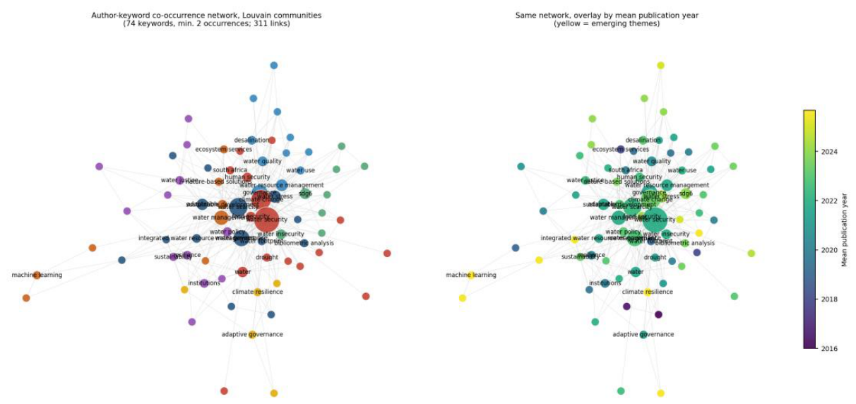
Figure A2.
Document similarity network of the 177 records, built on TF-IDF cosine similarity of titles, keywords and abstracts. Node colour marks the thematic cluster, node size the citation count.
Figure A2.
Document similarity network of the 177 records, built on TF-IDF cosine similarity of titles, keywords and abstracts. Node colour marks the thematic cluster, node size the citation count.
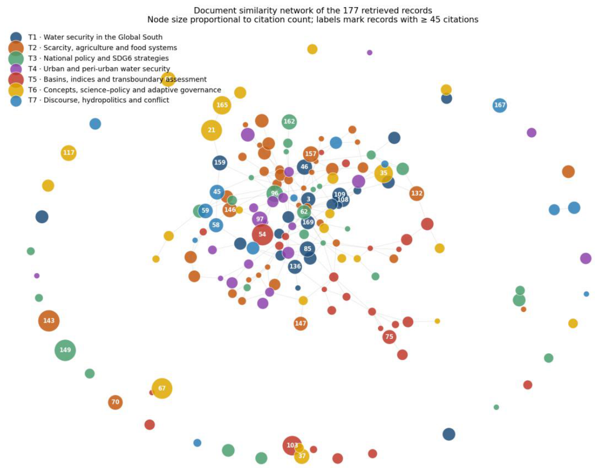
Figure A3.
Descriptives of the collected records: annual output, leading outlets, and size of the seven thematic clusters.
Figure A3.
Descriptives of the collected records: annual output, leading outlets, and size of the seven thematic clusters.
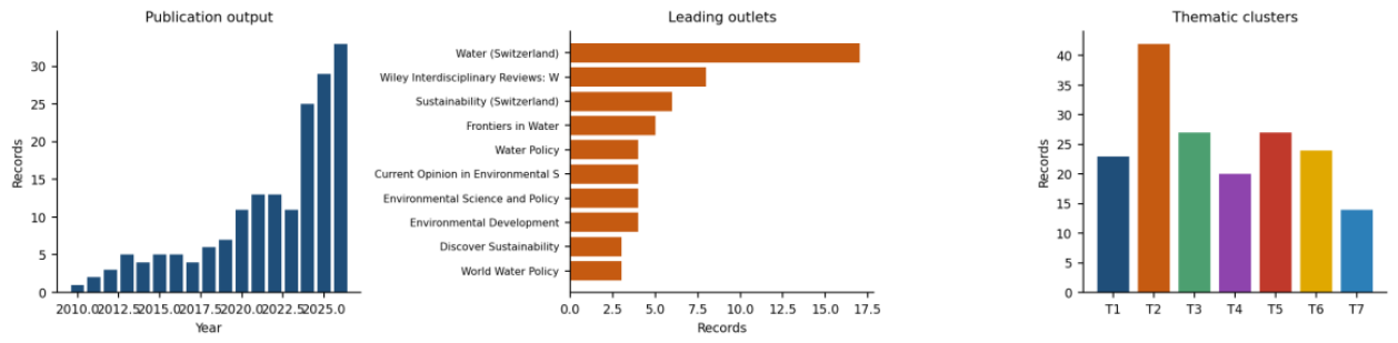
Appendix B. Robustness of the Governance Equation
The lower tail of the second principal component of the Worldwide Governance Indicators — high administrative capacity relative to accountability — is occupied almost entirely by hydrocarbon exporters of the Gulf and the wider Middle East and North Africa, and these are also among the most arid economies in the sample. Two explanations of the accountability contrast reported in Section 10 are therefore observationally close: that economies with capacity running ahead of accountability carry higher water stress, or that they are simply drier. This appendix separates them with two complementary checks — removing the economies that anchor the tail, and controlling for aridity directly.
The first restriction excludes the six members of the Gulf Cooperation Council, whose period-mean withdrawal ratios range from 107 to 1,689 per cent. The second additionally excludes fourteen further economies of the Middle East and North Africa, removing twenty countries in total, on the grounds that excluding the Gulf alone leaves Egypt, Iran, Iraq, Morocco and Tunisia in the same tail.
Table A1.
Orthogonalised governance equation on the full sample and on two regionally restricted samples.
Table A1.
Orthogonalised governance equation on the full sample and on two regionally restricted samples.
| Sample | Estimator | Institutional quality (PC1) |
Institutional balance (PC2) |
Female/male LFP ratio |
Sci. articles pc (ln) |
N | Econ. | R² |
|---|---|---|---|---|---|---|---|---|
| Full sample | Pooled OLS | 0.0195 (0.0924) | -0.9731*** (0.2395) | -0.0396*** (0.0052) | 0.1854** (0.0848) | 3,421 | 170 | 0.3614 |
| Fixed effects | 0.0032 (0.0282) | -0.0094 (0.0365) | -0.0015 (0.0030) | 0.0694*** (0.0233) | 3,421 | 170 | 0.0266 | |
| Between | 0.0481 (0.1287) | -1.1044*** (0.3092) | -0.0397*** (0.0057) | 0.1979* (0.1159) | 3,421 | 170 | 0.3745 | |
| Excluding GCC | Pooled OLS | 0.0114 (0.0914) | -0.6796*** (0.2506) | -0.0367*** (0.0053) | 0.2035** (0.0839) | 3,295 | 164 | 0.2837 |
| Fixed effects | -0.0004 (0.0290) | -0.0166 (0.0372) | -0.0016 (0.0032) | 0.0722*** (0.0241) | 3,295 | 164 | 0.0274 | |
| Between | 0.0732 (0.1278) | -0.8296** (0.3210) | -0.0375*** (0.0057) | 0.2391** (0.1140) | 3,295 | 164 | 0.2961 | |
| Excluding MENA | Pooled OLS | 0.0715 (0.0887) | -0.6729** (0.2698) | -0.0311*** (0.0079) | 0.1616* (0.0898) | 3,013 | 150 | 0.1797 |
| Fixed effects | 0.0138 (0.0306) | -0.0361 (0.0386) | -0.0027 (0.0035) | 0.0794*** (0.0252) | 3,013 | 150 | 0.0362 | |
| Between | 0.1254 (0.1194) | -0.7254** (0.3379) | -0.0314*** (0.0083) | 0.2152* (0.1236) | 3,013 | 150 | 0.1930 |
Note. GDP growth and internet penetration are included throughout and omitted for space; neither is significant in any column. GCC denotes Saudi Arabia, the United Arab Emirates, Qatar, Kuwait, Bahrain and Oman; MENA additionally denotes Algeria, Egypt, Iran, Iraq, Jordan, Lebanon, Libya, Morocco, Syria, Tunisia, Yemen, Israel, Türkiye and Malta. Country-clustered standard errors in parentheses for pooled OLS and fixed effects, robust standard errors for the Between estimator. *** p < 0.01, ** p < 0.05, * p < 0.10.
The Between coefficient on institutional balance falls from −1.1044 to −0.8296 without the Gulf and to −0.7254 without the wider region, an attenuation of 25 and 34 per cent, and remains significant at five per cent in both. The raw cross-sectional correlation with log water stress follows the same path, from −0.427 to −0.298 and then −0.223. The null on institutional quality is unaffected and drifts towards the sign opposite to the conventional prior. The female-to-male participation ratio retains significance at one per cent throughout, and the Between R² falls from 0.3745 to 0.1930 — what the governance pillar explains in the cross-section is in large part the position of one identifiable group of economies.
Exclusion removes the confound by removing the observations, at the cost of the range that identifies the coefficient. The complementary approach retains the full sample and admits aridity as a regressor. The measure is the period mean of the Standardised Precipitation-Evapotranspiration Index, reversed in sign and standardised so that higher values denote drier territories, available for 169 of the 170 economies. It is a country attribute rather than a time-varying one and therefore drops out under the within transformation. Its correlation with institutional balance across country means is -0.18, low enough that the two enter the same specification without difficulty. Column (3) adds the interaction, which asks whether the contrast operates differently in arid and humid territories, and column (4) combines the interaction specification with the Gulf exclusion of Table A1.
Table A2.
Governance equation with aridity and its interaction with institutional balance.
| (1) baseline |
(2) + aridity |
(3) + interaction |
(4) (3), excl. GCC |
|
|---|---|---|---|---|
| Panel A. Between estimator | ||||
| Institutional quality (PC1) | 0.0499 (0.1286) |
0.1410 (0.1192) |
0.1400 (0.1202) |
0.1537 (0.1206) |
| Institutional balance (PC2) | -1.1078*** (0.3090) |
-1.0657*** (0.2759) |
-1.0033*** (0.2752) |
-0.9659*** (0.2964) |
| Aridity | — | 0.4662*** (0.1332) |
0.4160*** (0.1459) |
0.3747** (0.1455) |
| Institutional balance × aridity | — | — | -0.2564 (0.1973) |
-0.1799 (0.2648) |
| Female/male LFP ratio | -0.0398*** (0.0057) |
-0.0328*** (0.0061) |
-0.0317*** (0.0063) |
-0.0325*** (0.0063) |
| Sci. articles pc (ln) | 0.1928 (0.1175) |
0.1069 (0.1192) |
0.1326 (0.1209) |
0.1506 (0.1233) |
| N | 3,400 | 3,400 | 3,400 | 3,274 |
| Economies | 169 | 169 | 169 | 163 |
| R² | 0.3750 | 0.4299 | 0.4347 | 0.3376 |
| Panel B. Pooled OLS | ||||
| Institutional quality (PC1) | 0.0231 (0.0929) |
0.1080 (0.0846) |
0.0996 (0.0849) |
0.0906 (0.0853) |
| Institutional balance (PC2) | -0.9827*** (0.2419) |
-0.9522*** (0.2092) |
-0.8937*** (0.2145) |
-0.7986*** (0.2319) |
| Aridity | — | 0.4799*** (0.1294) |
0.4374*** (0.1384) |
0.3852*** (0.1379) |
| Institutional balance × aridity | — | — | -0.2235 (0.1697) |
-0.0748 (0.2198) |
| Female/male LFP ratio | -0.0397*** (0.0052) |
-0.0321*** (0.0057) |
-0.0310*** (0.0058) |
-0.0317*** (0.0058) |
| Sci. articles pc (ln) | 0.1817** (0.0858) |
0.1062 (0.0848) |
0.1214 (0.0844) |
0.1321 (0.0859) |
| N | 3,400 | 3,400 | 3,400 | 3,274 |
| Economies | 169 | 169 | 169 | 163 |
| R² | 0.3620 | 0.4196 | 0.4239 | 0.3247 |
Note. Aridity is the reversed, standardised period mean of the Standardised Precipitation-Evapotranspiration Index; higher values denote drier territories. GDP growth and internet penetration are included throughout and omitted for space. Standard errors in parentheses. *** p < 0.01, ** p < 0.05, * p < 0.10.
Table A3.
Marginal effect of institutional balance on log water stress across the aridity distribution, Between estimator, column (3).
Table A3.
Marginal effect of institutional balance on log water stress across the aridity distribution, Between estimator, column (3).
| Aridity level | Standardised value |
Marginal effect | Standard error |
t |
|---|---|---|---|---|
| Very humid | -1.5 | -0.6187 | 0.4615 | -1.34 |
| Humid | -1.0 | -0.7469* | 0.3844 | -1.94 |
| Sample mean | +0.0 | -1.0033*** | 0.2752 | -3.65 |
| Arid | +1.0 | -1.2598*** | 0.2856 | -4.41 |
| Very arid | +2.0 | -1.5162*** | 0.4065 | -3.73 |
Entered directly, aridity carries +0.4662 in the Between estimator and +0.4799 in pooled OLS, both at one per cent, and raises the Between R² from 0.3750 to 0.4299. A one standard deviation increase in dryness is associated with roughly a 59 per cent increase in the withdrawal-to-resource ratio. The physical confound the paper worried about is real and large.
Controlling for aridity moves the Between coefficient on institutional balance only from −1.1078 to −1.0657, an attenuation of under four per cent, and it remains significant at one per cent. This is the decisive comparison in the appendix: removing the arid economies attenuated the contrast by a quarter, whereas measuring their aridity and holding it constant barely moves it. The two results together imply that the attenuation in Table A1 is a consequence of losing the range that identifies the coefficient rather than of removing a confound.
The interaction is negative but insignificant, at −0.2564 with a standard error of 0.1973. Table A3 shows the marginal effect steepening monotonically from −0.62 in the most humid territories to −1.52 in the most arid, but the difference across that range is not statistically distinguishable. The relationship is additive: aridity and institutional composition each carry an independent association with water stress, and neither conditions the other.
Column (4) controls for aridity and excludes the Gulf simultaneously. The Between coefficient on institutional balance is −0.9659, significant at one per cent, against −1.0033 with the Gulf retained — an attenuation of under four per cent once aridity is held constant, rather than the twenty-five per cent of Table A1. Institutional quality remains null throughout all four columns.
Appendix C. Cross-Sectional Dependence
The Pesaran statistic on fixed-effects residuals is 23.44 on the environmental block and 6.93 on the governance block, in both cases rejecting cross-sectional independence at any conventional level. This is expected: countries drawing on the Nile, the Mekong or the Indus cannot have independent error terms, and all economies are exposed to common global shocks in commodity prices, climate and macroeconomic conditions. Country-clustered standard errors, used throughout the paper, allow arbitrary correlation within a country over time but assume independence across countries, and are therefore not robust to this feature of the data.
The standard remedy is the Driscoll–Kraay covariance estimator, which averages the moment conditions cross-sectionally at each date and then applies a heteroskedasticity and autocorrelation consistent correction over time. Its asymptotics run in the time dimension, and the panels estimated here have twenty-two and twenty-one periods against 166 and 170 economies. Applied to this panel shape the estimator is anti-conservative rather than conservative.
Table A4.
Standard errors on two representative coefficients under alternative covariance estimators, fixed effects.
Table A4.
Standard errors on two representative coefficients under alternative covariance estimators, fixed effects.
| Block | Covariance estimator | Coefficient | Standard error | t |
|---|---|---|---|---|
| Environmental | Country-clustered | 0.3430 | 0.1327 | 2.58 |
| Two-way clustered | 0.3430 | 0.1313 | 2.61 | |
| Driscoll–Kraay, bw = 1 | 0.3430 | 0.0241 | 14.24 | |
| Driscoll–Kraay, bw = 2 | 0.3430 | 0.0270 | 12.69 | |
| Driscoll–Kraay, bw = 3 | 0.3430 | 0.0287 | 11.93 | |
| Driscoll–Kraay, bw = 5 | 0.3430 | 0.0301 | 11.41 | |
| Driscoll–Kraay, bw = 8 | 0.3430 | 0.0306 | 11.22 | |
| Governance | Country-clustered | 0.0694 | 0.0233 | 2.98 |
| Two-way clustered | 0.0694 | 0.0243 | 2.86 | |
| Driscoll–Kraay, bw = 1 | 0.0694 | 0.0115 | 6.06 | |
| Driscoll–Kraay, bw = 2 | 0.0694 | 0.0125 | 5.56 | |
| Driscoll–Kraay, bw = 3 | 0.0694 | 0.0137 | 5.05 | |
| Driscoll–Kraay, bw = 5 | 0.0694 | 0.0147 | 4.70 | |
| Driscoll–Kraay, bw = 8 | 0.0694 | 0.0147 | 4.73 |
Note. The reported coefficient is population density in the environmental block and scientific articles per capita in the governance block. The point estimate is identical across rows; only the covariance estimator changes. bw denotes the Newey–West bandwidth.
Driscoll–Kraay standard errors are between three and five times smaller than country-clustered ones at every bandwidth, turning a t statistic of 2.58 into one of 12.69 and a t statistic of 2.98 into one of 5.56. The direction is systematic and it is a property of the panel shape rather than of these two coefficients: cross-sectional averaging removes the idiosyncratic country variation that clustering preserves, and the subsequent time-series correction is computed on twenty-two observations. Reporting these figures would make every result in the paper more significant while addressing none of the dependence that motivated the check. They are shown here so that the choice not to use them is documented rather than silent. Two-way clustering, by contrast, changes the standard errors by less than two per cent.
Appendix D. Comparing the Three Pillars on a Common Sample
Section 13 ranks the three pillars by how much of the variation in water stress each explains. That comparison is made across equations estimated on different countries: the environmental and governance blocks cover 170 economies, the social block only 99, because safely managed drinking water and sanitation are reported for 148 and 143 countries respectively. The economies missing from the social block are not missing at random — they are on average poorer or more arid, and they include the Gulf exporters that occupy the upper tail of the dependent variable — so a lower between-country R² on the social block is exactly what removing them would produce whatever that pillar explains.
The main estimates remain those reported in Section 4 and Section 10, on the largest sample each block supports; restricting them would discard information for no gain. What the ranking requires is a like-for-like comparison, and this appendix supplies it by re-estimating the environmental and governance equations on the 99 economies of the social sample.
Table A5.
Explanatory performance of the three blocks on their own samples and on the common sample of 99 economies.
Table A5.
Explanatory performance of the three blocks on their own samples and on the common sample of 99 economies.
| Block | Sample | N | Econ. | Within R² | Between R² | Pooled R² | Variance: between / within (%) |
|---|---|---|---|---|---|---|---|
| Environmental | Full | 3,463 | 166 | 0.0651 | 0.4892 | 0.4599 | 99.0 / 1.0 |
| Common | 2,081 | 98 | 0.0805 | 0.4317 | 0.3969 | 98.8 / 1.2 | |
| Social | Full = common | 2,113 | 99 | 0.1092 | 0.3034 | 0.2759 | — |
| Governance | Full | 3,421 | 170 | 0.0266 | 0.3745 | 0.3614 | 99.1 / 0.9 |
| Common | 2,024 | 99 | 0.0148 | 0.3915 | 0.3515 | 98.9 / 1.1 |
Note. The common sample restricts the environmental and governance equations to the economies of the social estimation sample; 98 of the 99 appear in the environmental panel. The within R² is from the fixed-effects estimator, the between R² from the between estimator. The final column reports the decomposition of the variance of log water stress itself, not of the fitted values. Environmental figures are computed on a reconstruction of the estimation sample that reproduces the published coefficients to three decimal places.
Both orderings survive the restriction. On the published samples the within-country ranking is social, environmental, governance, and the between-country ranking is environmental, governance, social. On the common sample the within ranking is 0.1092, 0.0805 and 0.0148, and the between ranking is 0.4317, 0.3915 and 0.3034. Neither ordering changes, and the comparison in Section 13 can therefore be stated without qualification.
The restriction moves the two blocks in opposite directions, and the movements are informative. The environmental block loses between-country explanatory power, from 0.4892 to 0.4317, and gains within-country power, from 0.0651 to 0.0805. Removing the arid and the very poor compresses the cross-sectional range on which forest cover and the drought index operate while leaving the density channel intact. The governance block does the reverse, gaining slightly between countries, from 0.3745 to 0.3915, and falling by nearly half within them, from 0.0266 to 0.0148. The within figure was close to zero on either sample and no reading in the paper depends on it.
The headline variance decomposition is not a sample artefact. The share of the variance of log water stress lying between countries is 99.0 and 99.1 per cent on the full environmental and governance samples, and 98.8 and 98.9 per cent on the common sample. The central structural claim of the paper holds on any of the four panels.
One caveat remains. The common sample is the social sample, so the comparison establishes that the ranking is not an artefact of who is in the environmental and governance panels. It cannot establish the converse, since the social block cannot be estimated on the 71 economies it lacks. The ranking is therefore robust to sample composition within the set of countries where all three blocks are observed, which is the strongest statement the data support.
References
- Xenarios, S.; Assubayeva, A.; Xie, L.; Sehring, J.; Amirkhanov, D.; Sultanov, A.; Fazli, S. A bibliometric review of the water security concept in Central Asia. Environmental Research Letters 2020, 16 (1), 013001. [CrossRef]
- Gajurel, S.; Maheshwari, B.; Hagare, D.; Ward, J.; Singh, P.K. Evolving research on groundwater governance and collective action for water security: A Global bibliometric analysis. Groundwater for Sustainable Development 2024, 26, 101224. [CrossRef]
- Sarker, J.; Rolfe, J.; Akbar, D. Mapping the Landscape: A Bibliometric Analysis of Water Security, Governance, and Trading in Australia. Water (Switzerland) 2025, 17 (7), 1035. [CrossRef]
- Sun, S.; Zheng, X.; Liu, X.; Wang, Z.; Liang, L. Global pattern and drivers of water scarcity research: a combined bibliometric and geographic detector study. Environmental Monitoring and Assessment 2022, 194 (8), 523. [CrossRef]
- Schuster, K.; Lima-Rezende, C.; Gonçalves, J.; de Souza Rezende, R. Advancing Water Security in the Tropical and Subtropical Regions: An Integrative Topic Modeling Approach. World Water Policy 2026, 12 (1), e70050. [CrossRef]
- Hussain, Z.; Wang, Z.; Yang, H.; Arfan, M.; Wang, W.; Faisal, M.; Azam, M.I.; Usman, M. Evolution and Trends of Water Scarcity Indicators: Unveiling Gaps, Challenges, and Collaborative Opportunities. Water Conservation Science and Engineering 2024, 9 (1), 8. [CrossRef]
- Bhargavan, J.; Ayikkara Kizhakkayil, K. The Evolution of Potable Water Security: A Temporal Analysis of Key Indices and Trends. Water (Switzerland) 2024, 16 (21), 3023. [CrossRef]
- Conway, D. Water on the mind: Mapping behavioral and psychological research on water security. Wiley Interdisciplinary Reviews: Water 2024, 11 (6), e1755. [CrossRef]
- Stringer, L.C.; Mirzabaev, A.; Benjaminsen, T.A.; Harris, R.M.B.; Jafari, M.; Lissner, T.K.; Stevens, N.; Tirado-von der Pahlen, C. Climate change impacts on water security in global drylands. One Earth 2021, 4 (6), 851–864. [CrossRef]
- Aggarwal, A.; Frey, H.; McDowell, G.; Drenkhan, F.; Nüsser, M.; Racoviteanu, A.; Hoelzle, M. Adaptation to climate change induced water stress in major glacierized mountain regions. Climate and Development 2022, 14 (7), 665–677. [CrossRef]
- Isaacman, A.; Musemwa, M. Water security in africa in the age of global climate change. Daedalus 2021, 150 (4), 7–26. [CrossRef]
- John, C.K.; Pu, J.H. Climate-Driven Water Scarcity and Its Public Health Implications: A Multi-Regional Assessment Across Vulnerable Socio-Ecological Systems. Water (Switzerland) 2026, 18 (6), 699. [CrossRef]
- Mena, N.; Awange, J.; Mi, X. Managing the Nile under climate change: A systematic review of hydrological shifts and adaptive strategies for transboundary water security. Journal of Hydrology: Regional Studies 2026, 66, 103678. [CrossRef]
- Ndlovu, S.; Maviza, G. A systematic review of the impact of climate-related displacements on food and water security in Mozambique and Zimbabwe. Jamba: Journal of Disaster Risk Studies 2026, 18 (1), a1965. [CrossRef]
- Chen, L.; Xia, X.; Zhang, J.; Yan, X.; Wang, Z. Future food security risks driven by crop production and water scarcity in China's Yangtze River Delta under SSP–RCP scenarios. Ecological Indicators 2026, 189, 115209. [CrossRef]
- Jain, S.K.; Saharia, M.; Murty Bhallamudi, S.; Philip, L. Climate resilient development for sustainable water security for India. Current Science 2025, 128 (10), 969–986. [CrossRef]
- Matimolane, S.; Mathivha, F.I. Tackling rural water scarcity in South Africa: climate change, governance, and sustainability pathways. Frontiers in Environmental Science 2025, 13, 1550738. [CrossRef]
- Shah, A.; Karim, R.; Ali, K. Review of impacts of climate changes on the urban water security of Islamabad, Pakistan. Journal of Water and Land Development 2022, 54, 109–115. [CrossRef]
- Boretti, A. Covid19 pandemic as a further driver of water scarcity in Africa. GeoJournal 2022, 87 (2), 787–814. [CrossRef]
- Pérez, P.A.; Quiroz, W.; Echeveste, P. Coupled pollution and water scarcity heighten ecological degradation and social vulnerability in global dryland rivers. Environmental Research 2026, 293, 123708. [CrossRef]
- Mukherjee, S.; Bebermeier, W.; Schütt, B. An overview of the impacts of land use land cover changes (1980-2014) on urban water security of Kolkata. Land 2018, 7 (3), 91. [CrossRef]
- Keys, P.W.; Porkka, M.; Wang-Erlandsson, L.; Fetzer, I.; Gleeson, T.; Gordon, L.J. Invisible water security: Moisture recycling and water resilience. Water Security 2019, 8, 100046. [CrossRef]
- Posada-Marín, J.; Salazar, J.; Rulli, M.C.; Wang-Erlandsson, L.; Jaramillo, F. Upwind moisture supply increases risk to water security. Nature Water 2024, 2, 875–888. [CrossRef]
- Navarro-Ortega, A.; Acuña, V.; Bellin, A.; Burek, P.; Cassiani, G.; Choukr-Allah, R.; Dolédec, S.; Elosegi, A.; Ferrari, F.; Ginebreda, A.; et al. Managing the effects of multiple stressors on aquatic ecosystems under water scarcity. The GLOBAQUA project. Science of the Total Environment 2015, 503-504, 3–9. [CrossRef]
- Citrini, A.; Scanlon, B.R.; Rateb, A.; Zhao, G.; Sangiorgio, M.; Rosa, L. Global managed aquifer recharge potential as a solution to water scarcity. Nature Water 2026. [CrossRef]
- Paiva, A.C.D.E.; Martins, M.; Canamary, E.A.; Rodriguez, D.A.; Tomasella, J. Inter-basin water transfers under changing climate and land use: Assessing water security and hydropower in the Paraíba do Sul River basin, Brazil. Journal of South American Earth Sciences 2024, 133, 104707. [CrossRef]
- Marques, É.T.; Gunkel, G.; Sobral, M.C. Management of tropical river basins and reservoirs under water stress: Experiences from northeast Brazil. Environments - MDPI 2019, 6 (6), 62. [CrossRef]
- Kherazi, F.Z.; Sun, D.; Sohu, J.M.; Rhadiouini, C.E.; Shaikh, S.N. Mapping Urban Water Stress and Human-Water Conflicts: a Climate–Ecosystem Framework for Sustainable Water Management. Water Resources Management 2026, 40 (3), 99. [CrossRef]
- Abera, L.E.; Jumani, S.; van Rees, C.B.; Krishnaswamy, J.; Seigerman, C.K.; Nelson, D.R.; Hallemeier, J.; Mulatu, D.W.; Arora, R.; Sesma, M.P.V.; et al. Integrating Nature-based Solutions for urban water security in global south. PLOS Water 2025, 4 (6 June), e0000372. [CrossRef]
- Suman, D.O.; Morais, M.; Saito, C.H. Solutions Based on Nature to Face Water Stress: Lessons from the Past and Present. Water (Switzerland) 2024, 16 (16), 2301. [CrossRef]
- Peláez-Sánchez, S.; Sánchez, C.; Marijuan, R.; Díez, B.; Papadopoulou, O.; Poveda, P.M.; Valero, A.F.A.; Saugar, J.I.; Sánchez, R.; Martín, I.; et al. Bridging the IUCN Global Standard with governance and engagement tools: multi-method lessons from five Mediterranean case studies for strengthening water security. Nature-Based Solutions 2026, 9, 100327. [CrossRef]
- Mohd Nazir, N.Z.; Lee, K.E.; Goh, T.L.; Mokhtar, M.; Sharani, N.A.; Mohd Aris, A.; Khor, B.C.; Wan Abdullah, W.A.R.; Husain, H.; Raja Mamat, R.B. Enhancing water security through mobile constructed wetlands: A decentralised approach for wastewater reclamation and reuse. Journal of Environmental Chemical Engineering 2025, 13 (5), 117859. [CrossRef]
- Ricart, S.; Villar-Navascués, R.A.; Hernández-Hernández, M.; Rico-Amorós, A.M.; Olcina-Cantos, J.; Moltó-Mantero, E. Extending natural limits to address water scarcity? The role of non-conventional water fluxes in climate change adaptation capacity: A review. Sustainability (Switzerland) 2021, 13 (5), 2473. [CrossRef]
- Vörösmarty, C.J.; Stewart-Koster, B.; Green, P.A.; Boone, E.L.; Flörke, M.; Fischer, G.; Wiberg, D.A.; Bunn, S.E.; Bhaduri, A.; McIntyre, P.B.; et al. A green-gray path to global water security and sustainable infrastructure. Global Environmental Change 2021, 70, 102344. [CrossRef]
- Harshadeep, N.R.; Young, W. Disruptive technologies for improving water security in large river basins. Water (Switzerland) 2020, 12 (10), 2783. [CrossRef]
- Shemer, H.; Wald, S.; Semiat, R. Challenges and Solutions for Global Water Scarcity. Membranes 2023, 13 (6), 612. [CrossRef]
- Aleisa, E. Navigating Kuwait's water scarcity challenges: A holistic analysis of water resources, environmental impact, cost, and policy implications. Desalination 2024, 586, 117827. [CrossRef]
- Al-hasanat, A.; Chemack, F.; Sabbahi, S.; Nouiri, I.; Karanis, P.; Ben Ayed, L. Exploring treated wastewater reuse as an alternative option to cope with water scarcity: comparative review in Tunisia and Jordan. Water Practice and Technology 2025, 20 (12), 2881–2898. [CrossRef]
- Šteflová, M.; Koop, S.; Elelman, R.; Vinyoles, J.; Van Leeuwen, C.J.K. Governing non-potablewater-reuse to alleviate water stress: The case of Sabadell, spain. Water (Switzerland) 2018, 10 (6), 739. [CrossRef]
- Domnech, L.; Saurí, D. Socio-technical transitions in water scarcity contexts: Public acceptance of greywater reuse technologies in the Metropolitan Area of Barcelona. Resources, Conservation and Recycling 2010, 55 (1), 53–62. [CrossRef]
- Hope, R.; Foster, T.; Money, A.; Rouse, M. Harnessing mobile communications innovations for water security. Global Policy 2012, 3 (4), 433–442. [CrossRef]
- Kotzé, P. Investing in ecological infrastructure for our: Future water security. Water Wheel 2013, 12 (4), 23–27.
- Scruggs, C.E.; Heyne, C.M. Extending traditional water supplies in inland communities with nontraditional solutions to water scarcity. Wiley Interdisciplinary Reviews: Water 2021, 8 (5), e1543. [CrossRef]
- Bjornlund, H.; Wheeler, S. Water scarcity - Desperate solutions - Balancing the needs. Water and Energy International 2011, 68 (12), 46–54.
- Singh, A.K.; Mishra, S.; Singh, A.K.; Polavarapu, M.P.; Singh, A.K.; Madhav, S.; Singh, A.; Kumar, M.; Shukla, S.K. Global Water Scarcity: Understanding Challenges, Causes, and Mitigation Measures. Water Conservation Science and Engineering 2026, 11 (2), 78. [CrossRef]
- Gowri, V.; Thenmozhi, S.; Panneerselvam, A.S.; Vadivel, M.; Gupta, R.; Sathish Kumar, V. INTEGRATED STRATEGIES FOR ADDRESSING THE WATER SCARCITY. Journal of Environmental Protection and Ecology 2024, 25 (6), 2075–2085.
- Ali, O.A.; Siad, D.A.; Alasow, A.S.; Mohamed, A.D.; Abdullahi, A.Y.; Ali, A.A. From scarcity to sustainability: a review of the causes, consequences, and management strategies of water scarcity in Somalia. Discover Sustainability 2025, 6 (1), 927. [CrossRef]
- Anser, M.K.; Akhtar, M.Z.; Shah, S.T.H.; Khan, M.A.; Zaman, K. Water scarcity in Asian nations and the path to resilience. Asian Journal of Water, Environment and Pollution 2025, 22 (2), 140–151. [CrossRef]
- Gawel, E.; Bernsen, K. Do we really need a water footprint? Global trade, water scarcity and the limited role of virtualwater. GAIA 2011, 20 (3), 162–167. [CrossRef]
- Wang, Y.; Wang, X. Contrasting quantity and quality flows in China's intercity virtual water trade reshape water scarcity and inequality. Journal of Cleaner Production 2025, 531, 146878. [CrossRef]
- Qu, J.; Qin, C.; Wang, H.; Zhao, Y.; He, F.; Guan, Z.; Chang, H.; Shi, L. Water stress evolution and redistribution pathways under global inequality in consumption. Water Research 2026, 291, 125112. [CrossRef]
- Haqiqi, I.; Bowling, L.; Jame, S.; Baldos, U.; Liu, J.; Hertel, T. Global drivers of local water stresses and global responses to local water policies in the United States. Environmental Research Letters 2023, 18 (6), 065007. [CrossRef]
- Sinyolo, S.; Mudhara, M.; Wale, E. Water security and rural household food security: Empirical evidence from the Mzinyathi district in South Africa. Food Security 2014, 6 (4), 483–499. [CrossRef]
- Odekunle, F.J.; Fadeyi, A.A.; Fadairo, O.A.; Agbebiyi, M.J.; Igwilo, M.C.; Akindele-Sotunbo, D.B.; Alabi, A.S.; Adebayo, O.A.; Oyewole, K.A.; Akande, I.; et al. Resilient Food Systems in Water-Stressed Regions: A Comparative Analysis of Water Scarcity and Food Security in Botswana and South Africa. International Research Journal of Multidisciplinary Scope 2025, 6 (4), 561–579. [CrossRef]
- Hindiyeh, M.; Albatayneh, A.; AlAmawi, R. Water Energy Food Nexus to Tackle Future Arab Countries Water Scarcity. Air, Soil and Water Research 2023, 16. [CrossRef]
- Kucharik, C.J.; Booth, E.G.; Loheide S.P.,, II; Power, R.; Rissman, A.R.; Seifert, J.; Turner, M.G. Building US food-energy-water security requires avoiding unintended consequences for ecosystems. Frontiers in Ecology and the Environment 2023, 21 (5), 234–243. [CrossRef]
- Iwaniec, D.M.; Metson, G.S.; Cordell, D. P-FUTURES: Towards urban food & water security through collaborative design and impact. Current Opinion in Environmental Sustainability 2016, 20, 1–7. [CrossRef]
- Madaki, M.Y.; Ullah, A.; Ahado, S.; Agyemang, S.A.; Kofi, T.O.; Darr, D.; Bavorova, M. Small dams for climate Adaptation: Evidence from Ghana's one-village-one-dam program for water security and agro-pastoral resilience in semi-arid Africa. Journal of Environmental Management 2025, 393, 127164. [CrossRef]
- Leal Pacheco, F.A.; Tarlé Pissarra, T.C. Water security in the agriculture and cattle grazing activities: A systematic review. Water Security 2025, 26, 100191. [CrossRef]
- Mezouane, H.; Hank, D.; Delli, R. Agricultural Water Management under Water Scarcity in Algeria: Practices and Future Perspectives. Open Agriculture Journal 2026, 20. [CrossRef]
- Urquiza, A.; Billi, M. Water markets and social–ecological resilience to water stress in the context of climate change: an analysis of the Limarí Basin, Chile. Environment, Development and Sustainability 2020, 22 (3), 1929–1951. [CrossRef]
- Dragicevic, A.Z.; Afsharinia, B.; Gurtoo, A.; Stahn, H. RESILIENT FOOD-BIODIVERSITY OUTCOMES VIA STOCHASTIC CONTROL of MULTIPLEX SOCIO-ECOLOGICAL NETWORKS under WATER STRESS. Advances in Complex Systems 2026, 29 (01n02), 2550015. [CrossRef]
- Paudel, S.; Kumar, P.; Dasgupta, R.; Johnson, B.A.; Avtar, R.; Shaw, R.; Mishra, B.K.; Kanbara, S. Nexus between water security framework and public health: A comprehensive scientific review. Water (Switzerland) 2021, 13 (10), 1365. [CrossRef]
- Pittalis, C.; Kogoya, E.; Jaén Osuna, A.; Kambala, C. Uncovering the hidden implications of water scarcity for maternal health: a photovoice study in rural Malawi (Thyolo district). Frontiers in Global Women's Health 2025, 6, 1588219. [CrossRef]
- Wutich, A.; Jepson, W.E.; Stoler, J.; Thomson, P.; Kooy, M.; Brewis, A.; Staddon, C.; Meehan, K. A Global Agenda for Household Water Security: Measurement, Monitoring, and Management. Journal of the American Water Resources Association 2021, 57 (4), 530–538. [CrossRef]
- Wutich, A.; Thomson, P.; Jepson, W.; Stoler, J.; Cooperman, A.D.; Doss-Gollin, J.; Jantrania, A.; Mayer, A.; Nelson-Nuñez, J.; Walker, W.S.; et al. MAD water: Integrating modular, adaptive, and decentralized approaches for water security in the climate change era. Wiley Interdisciplinary Reviews: Water 2023, 10 (6), e1680. [CrossRef]
- Neog, K.; Bhuyan, M.J.; Deka, N. A novel participatory index-based approach to measuring household water security in Assam, India. International Journal of Water Resources Development 2026. [CrossRef]
- Kujinga, K.; Vanderpost, C.; Mmopelwa, G.; Wolski, P. An analysis of factors contributing to household water security problems and threats in different settlement categories of Ngamiland, Botswana. Physics and Chemistry of the Earth 2014, 67-69, 187–201. [CrossRef]
- Wutich, A. Water insecurity is human: why social science must be at the core of water security research and practice. Frontiers in Water 2024, 6, 1539170. [CrossRef]
- Ingutia, R. Who is being left behind in water security, where do they live, and why are they left behind towards the achievement of the 2030 agenda?. Sustainable Water Resources Management 2024, 10 (5), 168. [CrossRef]
- Khan, H.F.; Arshad, S.A. Beyond water scarcity: Water (in)security and social justice in Karachi. Journal of Hydrology: Regional Studies 2022, 42, 101140. [CrossRef]
- Owens, K.; Carmody, E.; Grafton, Q.; O'Donnell, E.; Wheeler, S.; Godden, L.; Allen, R.; Lyster, R.; Steduto, P.; Jiang, Q.; et al. Delivering global water security: Embedding water justice as a response to increased irrigation efficiency. Wiley Interdisciplinary Reviews: Water 2022, 9 (6), e1608. [CrossRef]
- Princea, S.K.; Lombea, C. Investigating water security and climate vulnerability in urban informal settlements: A case of kanyama township, lusaka, zambia; [Indagine sulla sicurezza idrica e la vulnerabilità climatica negli insediamenti informali urbani: Un caso del compound di Kanyama, Lusaka, Zambia]. Acque Sotterranee - Italian Journal of Groundwater 2025, 14 (4), 41–50. [CrossRef]
- Lazaro, L.L.B.; Abram, S.; Giatti, L.L.; Sinisgalli, P.; Jacobi, P.R. Assessing water scarcity narratives in Brazil – Challenges for urban governance. Environmental Development 2023, 47, 100885. [CrossRef]
- Thommandru, A.; Turdialiev, M.A.; Mone, V. Hydro-hegemony in the Anthropocene: Neoliberal Paradigms and Global South Marginalization in Water Scarcity Governance. Journal of Developing Societies 2025, 41 (3), 383–405. [CrossRef]
- Maharjan, M.; Chhetri, S.; Sinha, S.; Sharma, A.; Moula, M.M.; Poudel, K.; Sen, S.M.; Hossain, M.M.; Nowreen, S. Understanding water security in a peri-urban region: A study from two South Asian countries. APN Science Bulletin 2026, 15 (1), 219–236. [CrossRef]
- Chen, Y.; Bilton, A.M. Water Stress, Peri-Urbanization, and Community-Based Water Systems: A Reflective Commentary on the Metropolitan Area of Mexico City. Frontiers in Sustainable Cities 2022, 4, 790633. [CrossRef]
- Wilson, N.J.; Montoya, T.; Lambrinidou, Y.; Harris, L.M.; Pauli, B.J.; McGregor, D.; Patrick, R.J.; Gonzalez, S.; Pierce, G.; Wutich, A. From “trust” to “trustworthiness”: Retheorizing dynamics of trust, distrust, and water security in North America. Environment and Planning E: Nature and Space 2023, 6 (1), 42–68. [CrossRef]
- Tan, P.; Soleman Senda, S. From local wisdom to global ethics: a Spinozist reading of Barong Wae ritual of Manggarai community in Indonesia in the context of global water scarcity. Journal of Global Ethics 2026, 22 (1), 42–59. [CrossRef]
- Mutanda, G.W.; Nhamo, G. Gendered perspective on water security, rights and conflicts in sub-Saharan Africa: a systematic review. Frontiers in Water 2024, 6, 1399415. [CrossRef]
- Ototo, E.N.; Karanja, D.S.; Elliott, S.J. “If I was in charge”: A qualitative investigation of water security, gender-based violence and wellbeing in Kenya. Wellbeing, Space and Society 2024, 7, 100230. [CrossRef]
- Bacon, C.M.; Kelley, L.C.; Stewart, I.T. Toward a feminist political ecology of household food and water security during drought in northern Nicaragua. Ecology and Society 2022, 27 (1), 16. [CrossRef]
- Pahl-Wostl, C.; Palmer, M.; Richards, K. Enhancing water security for the benefits of humans and nature-the role of governance. Current Opinion in Environmental Sustainability 2013, 5 (6), 676–684. [CrossRef]
- Bogardi, J.J.; Dudgeon, D.; Lawford, R.; Flinkerbusch, E.; Meyn, A.; Pahl-Wostl, C.; Vielhauer, K.; Vörösmarty, C. Water security for a planet under pressure: Interconnected challenges of a changing world call for sustainable solutions. Current Opinion in Environmental Sustainability 2012, 4 (1), 35–43. [CrossRef]
- Wheater, H.S.; Gober, P. Water security and the science agenda. Water Resources Research 2015, 51 (7), 5406–5424. [CrossRef]
- Gerlak, A.K.; Mukhtarov, F. ‘Ways of knowing’ water: integrated water resources management and water security as complementary discourses. International Environmental Agreements: Politics, Law and Economics 2015, 15 (3), 257–272. [CrossRef]
- Ganoulis, J. A New Dialectical Model of Water Security under Climate Change. Water (Switzerland) 2023, 15 (14), 2672. [CrossRef]
- Jaeger, W.K.; Plantinga, A.J.; Chang, H.; Dello, K.; Grant, G.; Hulse, D.; McDonnell, J.J.; Lancaster, S.; Moradkhani, H.; Morzillo, A.T.; et al. Toward a formal definition of water scarcity in natural-human systems. Water Resources Research 2013, 49 (7), 4506–4517. [CrossRef]
- Norton, M.R. Water security: pipe dream or reality? A global perspective from the UK. Wiley Interdisciplinary Reviews: Water 2014, 1 (1), 11–18. [CrossRef]
- Larson, R.B. Water security. Northwestern University Law Review 2017, 112 (2), 139–200.
- De Carvalho, K.M. The global water security: An approach for multilevel governance on hydric resources. International Journal of Innovation and Sustainable Development 2019, 13 (1), 57–78. [CrossRef]
- Varady, R.G.; Zuniga-Teran, A.A.; Garfin, G.M.; Martín, F.; Vicuña, S. Adaptive management and water security in a global context: definitions, concepts, and examples. Current Opinion in Environmental Sustainability 2016, 21, 70–77. [CrossRef]
- Bettini, Y.; Brown, R.; De Haan, F.J. Water scarcity and institutional change: Lessons in adaptive governance from the drought experience of Perth, Western Australia. Water Science and Technology 2013, 67 (10), 2160–2168. [CrossRef]
- Devisscher, T.; Vignola, R.; Besa, M.C.; Cronenbold, R.; Pacheco, N.; Schillinger, R.; Canedi, V.; Sandoval, C.; Gonzalez, D.; Leclerc, G. Understanding the socio-institutional context to support adaptation for future water security in forest landscapes. Ecology and Society 2016, 21 (4), 48. [CrossRef]
- Flint, A.; Howard, G.; Nijhawan, A.; Poudel, M.; Geremew, A.; Mulugeta, Y.; Lo, E.; Ghimire, A.; Baidya, M.; Sharma, S. Managing climate change challenges to water security: Community water governance in Ethiopia and Nepal. Geo: Geography and Environment 2024, 11 (1), e00135. [CrossRef]
- Paul, D.; Thompson, B.S.; Farrelly, M. Expanding theories of learning for adaptive governance: Civil society action on water security and environmental pollution. Environmental Science and Policy 2025, 174, 104261. [CrossRef]
- Lutz-Ley, A.N.; Scott, C.A.; Wilder, M.; Varady, R.G.; Ocampo-Melgar, A.; Lara-Valencia, F.; Zuniga-Teran, A.A.; Buechler, S.; Díaz-Caravantes, R.; Ribeiro Neto, A.; et al. Dialogic science-policy networks for water security governance in the arid Americas. Environmental Development 2021, 38, 100568. [CrossRef]
- Adams, E.A.; Zulu, L.; Ouellette-Kray, Q. Community water governance for urban water security in the Global South: Status, lessons, and prospects. Wiley Interdisciplinary Reviews: Water 2020, 7 (5), e1466. [CrossRef]
- Groot, R.; Bayrak, M.M. Achieving water security in peri-urban Yangon: Exploring the local governance processes. Water Policy 2019, 21 (5), 980–998. [CrossRef]
- Agyeman, N.K.; Tantoh, H.B.; Kamika, I. Assessing water security and governance complexity in the Owabi river catchment in Ghana. Discover Sustainability 2026, 7 (1), 934. [CrossRef]
- LaVanchy, G.T.; Romano, S.T.; Taylor, M.J. Challenges to water security along the "emerald coast": A political ecology of localwater governance in Nicaragua. Water (Switzerland) 2017, 9 (9), 655. [CrossRef]
- Adom, R.K.; Simatele, M.D. Analysis of public policies and programmes towards water security in post-Apartheid South Africa. Water Policy 2021, 23 (3), 503–520. [CrossRef]
- Sershen; Rodda, N.; Stenström, T.A.; Schmidt, S.; Dent, M.; Bux, F.; Hanke, N.; Buckley, C.A.; Fennemore, C. Water security in South Africa: Perceptions on public expectations and municipal obligations, governance and water re-use. Water SA 2016, 42 (3), 456–465. [CrossRef]
- Chiquito Gesualdo, G.; Sone, J.S.; Galvão, C.D.O.; Martins, E.S.; Montenegro, S.M.G.L.; Tomasella, J.; Mendiondo, E.M. Unveiling water security in Brazil: current challenges and future perspectives. Hydrological Sciences Journal 2021, 66 (5), 759–768. [CrossRef]
- Cunha Libanio, P.A. Water reforms in Brazil: Challenges and opportunities for promoting water security in a continental-sized country. World Water Policy 2020, 6 (2), 230–245. [CrossRef]
- Ferreira, M.V.; Macedo, D.R.; Júnior, A.P.M. Divergent frameworks, shared challenges: a comparative analysis of National and State Water Security Plans in Minas Gerais, Brazil; [Estruturas divergentes, desafios compartilhados: uma análise comparativa dos Planos Nacional e Estadual de Segurança Hídrica em Minas Gerais, Brasil]. Revista Brasileira de Recursos Hidricos 2025, 30, e48. [CrossRef]
- Ishaque, W.; Mukhtar, M.; Tanvir, R. Pakistan’s water resource management: Ensuring water security for sustainable development. Frontiers in Environmental Science 2023, 11, 1096747. [CrossRef]
- Rowwad, A.A.; Mohammad, A.H. MANAGING WATER SCARCITY THROUGH POLICY AND INSTITUTIONAL REFORM: THE EVOLUTION OF WATER GOVERNANCE IN JORDAN. Water Conservation and Management 2025, 9 (4), 699–706. [CrossRef]
- Azemzi, H. Governance and policy approaches for addressing water scarcity: insights from Morocco. Euro-Mediterranean Journal for Environmental Integration 2025, 10 (4), 2431–2442. [CrossRef]
- Kaiss, R.; Benjouid, Z.; Faiz, M.; Ech-Chahed, H.; Rakhimi, A.; Zarouali, S.S.; Maimoun, A.; Hmid, A.; Cherkaoui, M. Water Stress and Regional Governance in Morocco: Pathways to Agricultural Resilience through Advanced Regionalization. Research on World Agricultural Economy 2025, 6 (3), 957–972. [CrossRef]
- Zhumasheva, S.; Yespolov, T.; Islamov, Y.; Kurmanova, G.; Iskakova, G.; Daniyarova, M. Analysis of the State of Water Resources, Water Use, and Water Security in the Agricultural Sector of Kazakhstan and Ways to Address Them. International Journal of Sustainable Development and Planning 2026, 21 (4), 1777–1788. [CrossRef]
- Jiang, Y. China's water security: Current status, emerging challenges and future prospects. Environmental Science and Policy 2015, 54, 106–125. [CrossRef]
- Ye, Q.; Chu, Z. Impact of water security policy coordination on water environment governance performance; [水安全政策协同对水环境治理绩效的影响]. Resources Science 2026, 48 (4), 999–1013. [CrossRef]
- Khalid, R.B.; Buhari, J.; Rosli, M.I.; Idris, M.I.; Abdullah, S.R.S. Water Security Management in Malaysia: Challenges, Technological Innovations, and Strategic Lessons from Global Practice. Water, Air, and Soil Pollution 2026, 237 (9), 509. [CrossRef]
- Salas-Bravo, S.; Bodini-Salas, A.; Araya-Piñones, A. Participatory scenario planning for sustainable development in San Pedro de Atacama, Chile: Addressing water scarcity and cultural preservation. Environmental Development 2026, 57, 101316. [CrossRef]
- Kies-Ryan, S. Creative and Innovative Approaches to Engaging With Communities in Water Security in the Solomon Islands. Asia Pacific Issues 2025, 29 (173).
- Gheuens, J.; Nagabhatla, N.; Perera, E.D.P. Disaster-risk, water security challenges and strategies in Small Island Developing States (SIDS). Water (Switzerland) 2019, 11 (4), 637. [CrossRef]
- Chin, S.; Ramnath, S.; Khan, K.; Elibox, W. A community resilience framework for water scarcity (CRFS) in the small Island developing country of Trinidad and Tobago. Sustainable Water Resources Management 2026, 12 (3), 44. [CrossRef]
- Abid, M.; Naqvi, S.A.; Ahmed, R.; Kamil, I.; Ahmad, M.; Qayyum, R.; Arshad, M. Technological Innovations in Water Security. Pakistan Journal of Engineering and Applied Sciences 2025, 33, 88–93.
- Mujtaba, G.; Shah, M.U.H.; Hai, A.; Daud, M.; Hayat, M. A holistic approach to embracing the United Nation's Sustainable Development Goal (SDG-6) towards water security in Pakistan. Journal of Water Process Engineering 2024, 57, 104691. [CrossRef]
- Marcal, J.; Antizar-Ladislao, B.; Hofman, J. Addressing water security: An overview. Sustainability (Switzerland) 2021, 13 (24), 13702. [CrossRef]
- Everard, M.; Sharma, O.P.; Vishwakarma, V.K.; Khandal, D.; Sahu, Y.K.; Bhatnagar, R.; Singh, J.K.; Kumar, R.; Nawab, A.; Kumar, A.; et al. Assessing the feasibility of integrating ecosystem-based with engineered water resource governance and management for water security in semi-arid landscapes: A case study in the Banas catchment, Rajasthan, India. Science of the Total Environment 2018, 612, 1249–1265. [CrossRef]
- Green, P.A.; Vörösmarty, C.J.; Koehler, D.A.; Brown, C.; Rex, W.; Rodriguez Osuna, V.; Tessler, Z. Mapping a sustainable water future: Private sector opportunities for global water security and resilience. Global Environmental Change 2024, 88, 102906. [CrossRef]
- Ragusa, A.T.; Crampton, A. Clicking and Swiping Away: Hidden Implications of Australian Data Center Water Security and Management. Water (Switzerland) 2026, 18 (2), 136. [CrossRef]
- de Castro-Pardo, M.; Fernández Martínez, P.; Pérez Zabaleta, A. An initial assessment of water security in Europe using a DEA approach. Sustainable Technology and Entrepreneurship 2022, 1 (1), 100002. [CrossRef]
- Link, P.M.; Scheffran, J.; Ide, T. Conflict and cooperation in the water-security nexus: a global comparative analysis of river basins under climate change. Wiley Interdisciplinary Reviews: Water 2016, 3 (4), 495–515. [CrossRef]
- Olanya, D.R. Land-Water-Security Nexus: Changing Geopolitics in the Nile Basin Cooperative Framework Agreement. Middle East Law and Governance 2017, 9 (1), 71–87. [CrossRef]
- Ribeiro, W.C.; Sant’Anna, F.M. Water security and interstate conflict and cooperation; [Seguretat hídrica i conflicte i cooperació interestatals]; [Sécurité hydrique, conflits et coopération inter-états]; [Seguridad hídrica y conflicto y cooperación interestatales]. Documents d'Analisi Geografica 2014, 60 (3), 573–596. [CrossRef]
- Saklani, U.; Shrestha, P.P.; Mukherji, A.; Scott, C.A. Hydro-energy cooperation in South Asia: Prospects for transboundary energy and water security. Environmental Science and Policy 2020, 114, 22–34. [CrossRef]
- Van That, V.; Loi, T.T.H.; Van, T.T.T.; Co, N.D. Water Security Issues in the Mekong River Basin: Current Situation and Vietnam’s Responses. Pakistan Journal of Life and Social Sciences 2024, 22 (2), 5677–5690. [CrossRef]
- Phuong, N.T.; Dung, M.Q. Assessing the Implementation of Commitments to Ensure Water Security among Mekong Subregional Countries (1995-2025). Journal of People, Plants, and Environment 2026, 29 (S1), 157–168. [CrossRef]
- Williams, J.M. Stagnant Rivers: Transboundary water security in South and Southeast Asia. Water (Switzerland) 2018, 10 (12), 1819. [CrossRef]
- Yang, J.; Huang, G. Study on the Mechanism of Multi-Scalar Transboundary Water Security Governance in the Shenzhen River. Sustainability (Switzerland) 2024, 16 (16), 7138. [CrossRef]
- Truong, T.H.; Nguyen, L.T.T.; Nguyen, D.D.; Pham, T.; Vu, T.M.; Nguyen, P.H.; Nguyen, Q.T. Water security assessment framework for deltas of the transboundary river basins. Global Journal of Environmental Science and Management 2023, 9 (3), 619–636. [CrossRef]
- Howlader, M.R. Hydrological hegemony and U.S. strategic engagement in climate and water security. Discover Global Society 2026, 4 (1), 21. [CrossRef]
- Zhifei, L. Water security in china’s neighboring diplomacy. China Quarterly of International Strategic Studies 2015, 1 (4), 625–646. [CrossRef]
- Hussein, H.; Natta, A.; Yehya, A.A.K.; Hamadna, B. Syrian refugees, water scarcity, and dynamic policies: How do the new refugee discourses impact water governance debates in Lebanon and Jordan?. Water (Switzerland) 2020, 12 (2), 325. [CrossRef]
- Hussein, H. Yarmouk, Jordan, and Disi basins: Examining the impact of the discourse of water scarcity in Jordan on transboundary water governance. Mediterranean Politics 2019, 24 (3), 269–289. [CrossRef]
- Powell, N.; Larsen, R.K.; Bruin, A.; Powell, S.; Elrick-Barr, C. Water security in times of climate change and intractability: Reconciling conflict by transforming security concerns into equity concerns. Water (Switzerland) 2017, 9 (12), 934. [CrossRef]
- Asaka, J.O.; Argomedo, D.W.; Jones, N.P. Climate change risks to water security: Exploring the interplay between climate change, water theft, and water (in)security. Water Policy 2024, 26 (4), 359–380. [CrossRef]
- Watson, I.; Schwak, J. Materiality, territory and sovereignty: Responding to contradictory water security issues in the mekong region. Asian International Studies Review 2020, 21 (1), 25–45. [CrossRef]
- Nie, T.; Jiang, X.; Deng, C.; Cai, W.; Lei, Y.; Gao, S. Analysis of the evolution of water culture and water security in the Weihe River Basin over a 100 year-period. Science of the Total Environment 2024, 920, 171066. [CrossRef]
- Nie, T.; Jiang, X.; Lei, Y.; Zhang, Y.; Fan, S.; Deng, C.; Li, Y.; Wang, J.; Su, X.; Liu, C. The feedback mechanism between water culture and water security in the Yellow River Basin. Ecological Indicators 2025, 180, 114330. [CrossRef]
- Rodríguez-Blásquez, Y.; Ticona, G.A.; Santos Santos, T.F.; Aedo-Quililongo, S.; Zamora, D.; Salazar, D.B.; Forni, L.; Alvarenga, M. Evaluating the Effectiveness of an Interactive Tool for Water Governance in Transboundary Basins: A Participation-Based Approach and Visualization of Water Security from a Vulnerability Perspective. Water (Switzerland) 2025, 17 (2), 278. [CrossRef]
- Sojamo, S.; Larson, E.A. Investigating food and agribusiness corporations as global water security, management and governance agents: The case of Nestlé, Bunge and Cargill. Water Alternatives 2012, 5 (3), 619–635.
- Sojamo, S.; Rudebeck, T. Corporate Engagement in Water Policy and Governance: A Literature Review on Water Stewardship and Water Security. Water Alternatives 2024, 17 (2), 292–324.
- Farooq, M.B.; Naveed, K.; Khalid, F.; Narayan, A.K.; Khudir, I.M. Examining the extent and quality of corporate water management disclosures in extremely high-water stress countries. Sustainability Accounting, Management and Policy Journal 2025, 16 (3), 705–735. [CrossRef]
- Bolognesi, T.; Gerlak, A.K.; Giuliani, G. Explaining and measuring social-ecological pathways: The case of global changes and water security. Sustainability (Switzerland) 2018, 10 (12), 4378. [CrossRef]
- Koirala, S.; Fang, Y.; Dahal, N.M.; Zhang, C.; Pandey, B.; Shrestha, S. Application of water poverty index (WPI) in spatial analysis of water stress in Koshi River Basin, Nepal. Sustainability (Switzerland) 2020, 12 (2), 727. [CrossRef]
- Nath, B.D.; Schuster-Wallace, C.J.; Dickson-Anderson, S.E. Headwater-to-consumer Drinking Water Security Assessment Framework and Associated Indicators for Small Communities in High-income Countries. Water Resources Management 2022, 36 (3), 805–834. [CrossRef]
- Legass, A.M.; Alamirew, T.; Gebrehiwot, S.G.; Haro-Monteagudo, D.; Tsegaye, L.; Begashaw, G.B. Assessing urban water security in Awash River Basin, Addis Ababa, and its surrounding towns using Integrated Urban Water S ecurity Index. Discover Sustainability 2026, 7 (1), 354. [CrossRef]
- Jabari, S.; Shahrour, I.; El Khattabi, J. Assessment of the urban water security in a severe water stress area-application to Palestinian Cities. Water (Switzerland) 2020, 12 (7), 2060. [CrossRef]
- Verre, F.; Kumar, K.; Berndtsson, R.; Hashemi, H. Redefining water scarcity through the integrated water strategic resilience index amid climate and conflict pressures. Scientific Reports 2026, 16 (1), 9088. [CrossRef]
- Shomar, B.; Rahman, M. How does water security look like in 2050? Critical elements from national to global perspectives. Water Security 2026, 28, 100204. [CrossRef]
- Ak, M.Y.; Benson, D. Assessing the water security effectiveness of integrated river basin management: Comparative case study analysis for lesson-drawing. Frontiers in Water 2022, 4, 1013588. [CrossRef]
- Dang, N.M.; Vien, L.N.; Tanim, A.H.; Gagnon, A.S.; Anh, D.T. A Framework Using Applied Process Analysis Methods to Assess Water Security in the Vu Gia–Thu Bon River Basin, Vietnam. Sustainability (Switzerland) 2024, 16 (13), 5749. [CrossRef]
- Hoekstra, A.Y.; Buurman, J.; Van Ginkel, K.C.H. Urban water security: A review. Environmental Research Letters 2018, 13 (5), 053002. [CrossRef]
- Mukherjee, S.; Sundberg, T.; Sikdar, P.K.; Schütt, B. An Integrated Quantitative Assessment of Urban Water Security of a Megacity in the Global South. Frontiers in Water 2022, 4, 834239. [CrossRef]
- Mukherjee, S.; Sundberg, T. A transdisciplinary and collaborative urban water security framework: Developed through an interdisciplinary study in Kolkata, India. World Water Policy 2023, 9 (3), 519–549. [CrossRef]
- Laauwen, M.; Koehler, J.; Greene, M.; Huitema, D. Cities under pressure: a global review of acute urban water scarcity governance. Environmental Research Letters 2026, 21 (14), 143002. [CrossRef]
- Romero-Gomez, G. Water security and the hydro-social cycle in Catalonia: Diagnosis and challenges for a country under pressure; [La sécurité hydrique et le cycle hydrosocial en Catalogne: diagnostic et défis pour un pays sous pression]; [La seguridad hídrica y el ciclo hidrosocial en Cataluña: diagnosis y retos para un país bajo presión]. Documents d'Analisi Geografica 2025, 72 (1), 27–49. [CrossRef]
- Vallino, E.; Ridolfi, L.; Laio, F. Measuring economic water scarcity in agriculture: a cross-country empirical investigation. Environmental Science and Policy 2020, 114, 73–85. [CrossRef]
- Nkiaka, E. Exploring the socioeconomic determinants of water security in developing regions. Water Policy 2022, 24 (4), 608–625. [CrossRef]
- Nkiaka, E.; Okpara, U.T.; Okumah, M. Food-energy-water security in sub-Saharan Africa: Quantitative and spatial assessments using an indicator-based approach. Environmental Development 2021, 40, 100655. [CrossRef]
- Nkiaka, E.; Bryant, R.G.; Okumah, M.; Gomo, F.F. Water security in sub-Saharan Africa: Understanding the status of sustainable development goal 6. Wiley Interdisciplinary Reviews: Water 2021, 8 (6), e1552. [CrossRef]
- Owjimehr, S.; Emami Meybodi, M.; Asadian Falahieh, K. The impact of socioeconomic factors on water stress: insights from global analysis. Water International 2024, 49 (6), 738–759. [CrossRef]
- Munir, S. Economic openness, institutional quality, and sectoral dynamics as determinants of water stress: Evidence from Pakistan's freshwater withdrawal (1999–2023). Cleaner Water 2025, 4, 100157. [CrossRef]
- Günal, C.N.; Erenel, D.; Peçe, H. Governance Matters: Reducing Water Stress through Effective Institutions in MENA Countries. Water Economics and Policy 2026, 2650007. [CrossRef]
- Gao, C. The Impact of Technological Innovation, Good Governance, and Green Energy on Water Stress in Developed and Developing Economies. Land Degradation and Development 2026, 37 (5), 1606–1621. [CrossRef]
- Bolognesi, T.; Marti, G.; Giuliani, G. Water security and human development: The role of size, footprint and governance. Ecological Economics 2026, 247, 109038. [CrossRef]
- Ayadi, E. When Does Water Scarcity Become a Sovereign Financial Risk? International Threshold Evidence on Sovereign Borrowing Costs. Resources 2026, 15 (6), 79. [CrossRef]
- Barbier, E.B.; Burgess, J.C. Economics of Water Scarcity and Efficiency. Sustainability (Switzerland) 2024, 16 (19), 8550. [CrossRef]
- Varghese, S.K.; Veettil, P.C.; Speelman, S.; Buysse, J.; Van Huylenbroeck, G. Estimating the causal effect of water scarcity on the groundwater use efficiency of rice farming in South India. Ecological Economics 2013, 86, 55–64. [CrossRef]
- Thapa, B.; Scott, C.A. Institutional strategies for adaptation to water stress in farmer-managed irrigation systems of Nepal. International Journal of the Commons 2019, 13 (2), 892–908. [CrossRef]
- Mouelhi, S.; Kanzari, S.; Ben Mariem, S.; Zemni, N. Towards a Classification of Tunisian Dams for Enhanced Water Scarcity Governance: Parametric or Non-Parametric Approaches?. Hydrology 2025, 12 (4), 96. [CrossRef]
- Rangel, G.C.; Alves, V.B.A.D.S.; Costa, I.P.D.A.; Moreira, M.Â.L.; Costa, A.P.D.A.; Santos, M.D.; Eckstrand, E.C. Efficient Naval Surveillance: Addressing Label Noise with Rockafellian Risk Minimization for Water Security. Water (Switzerland) 2025, 17 (3), 401. [CrossRef]
- Alamanos, A.; Xenarios, S.; Assubayeva, A.; Landis, C.F.M.; Dellis, K.; Koundouri, P. Systems-thinking innovations for water security. Frontiers in Water 2024, 6, 1492698. [CrossRef]
Figure 1.
Research design: one dependent variable, three ESG blocks, three analytical tracks. Note. Three equations share the log withdrawal-to-availability ratio and differ only in the regressor block. Each is estimated along all three tracks, yielding nine analyses. The social sample is smaller because sanitation and drinking water coverage are reported for fewer economies.
Figure 1.
Research design: one dependent variable, three ESG blocks, three analytical tracks. Note. Three equations share the log withdrawal-to-availability ratio and differ only in the regressor block. Each is estimated along all three tracks, yielding nine analyses. The social sample is smaller because sanitation and drinking water coverage are reported for fewer economies.
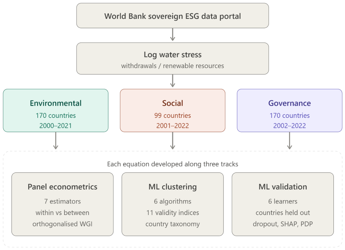
Figure 2.
Comparative performance of six clustering algorithms across the eleven internal validation indices. Notes. Cell values are the raw statistics; colour encodes the min–max normalised score, so that green marks the best-performing algorithm on each index.
Figure 2.
Comparative performance of six clustering algorithms across the eleven internal validation indices. Notes. Cell values are the raw statistics; colour encodes the min–max normalised score, so that green marks the best-performing algorithm on each index.
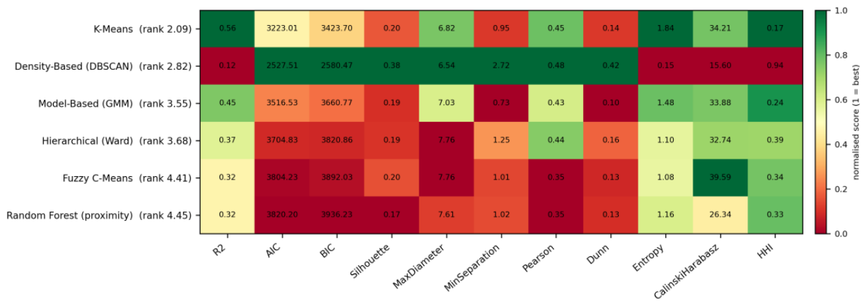
Figure 3.
Selection of the number of clusters for K-Means. Notes. The elbow in the within-cluster sum of squares, the plateau in the silhouette and Calinski–Harabasz curves, and the flattening of the information criteria jointly support k = 5 (dashed line).
Figure 3.
Selection of the number of clusters for K-Means. Notes. The elbow in the within-cluster sum of squares, the plateau in the silhouette and Calinski–Harabasz curves, and the flattening of the information criteria jointly support k = 5 (dashed line).
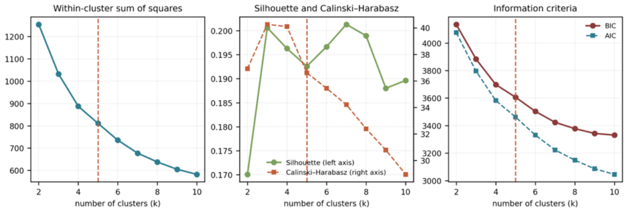
Figure 4.
K-Means partition in the space of the first two principal components, which jointly account for 51.9% of total variance. Note. Ellipses mark one and two standard deviations around each cluster centroid; arrows are the variable loadings.
Figure 4.
K-Means partition in the space of the first two principal components, which jointly account for 51.9% of total variance. Note. Ellipses mark one and two standard deviations around each cluster centroid; arrows are the variable loadings.
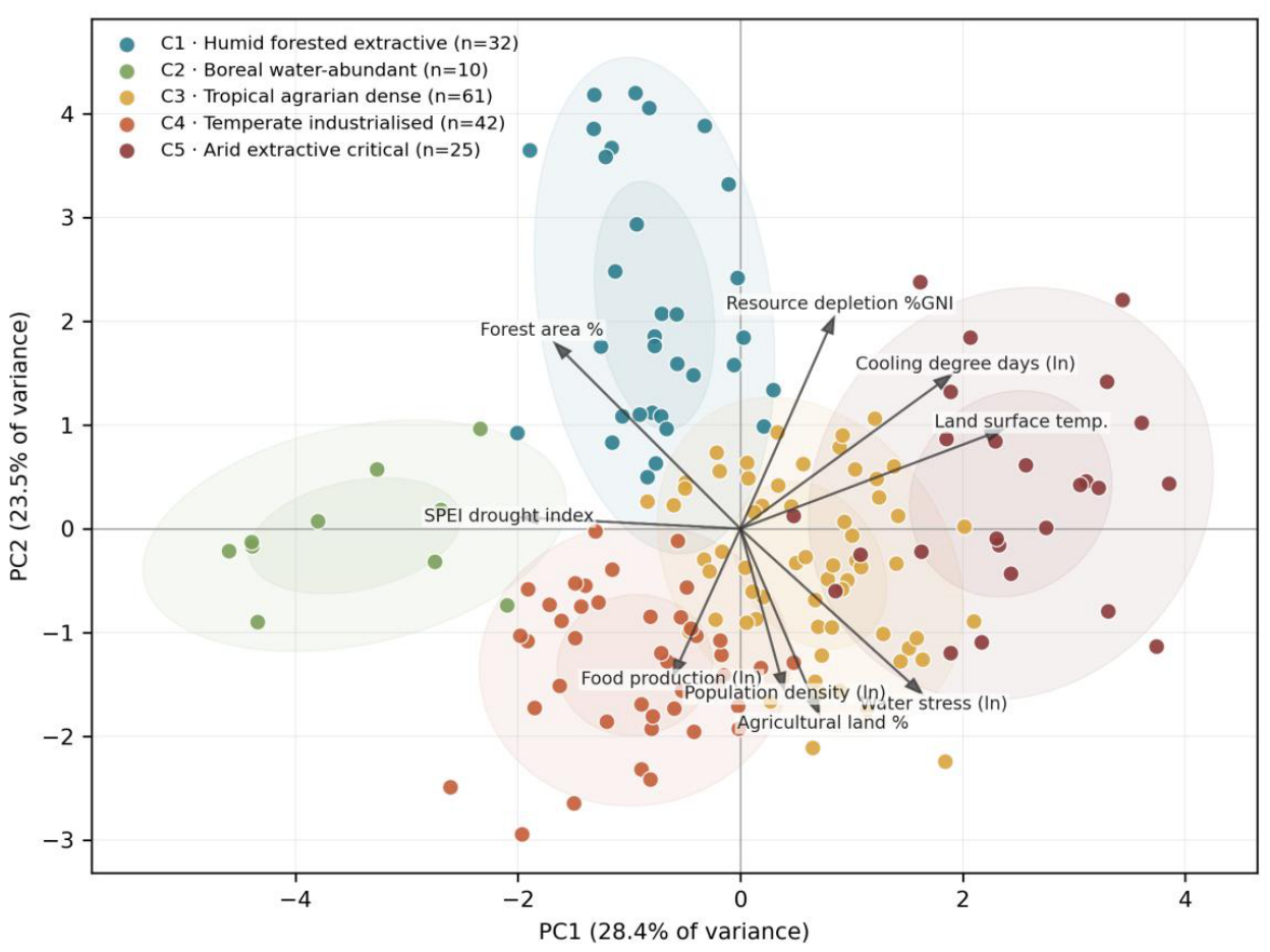
Figure 5.
Environmental profile of the five clusters. Notes. Cell values are cluster means expressed in standard deviations from the global mean, so that red marks values above and blue values below the cross-country average.
Figure 5.
Environmental profile of the five clusters. Notes. Cell values are cluster means expressed in standard deviations from the global mean, so that red marks values above and blue values below the cross-country average.
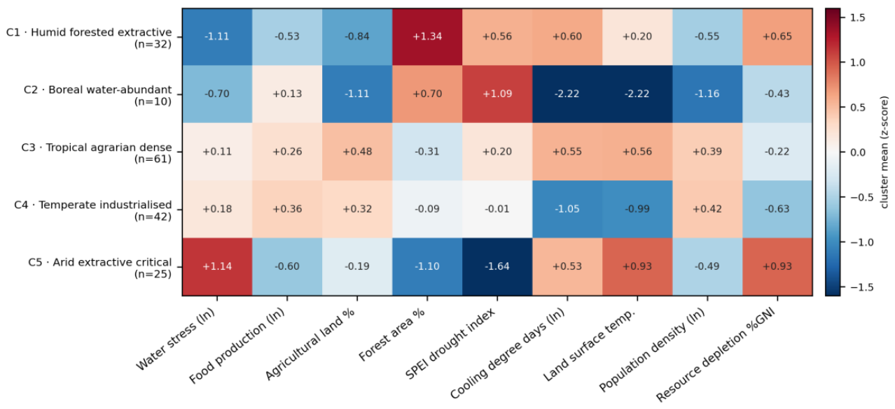
Figure 6.
Internal validity and outcome separation of the K-Means partition. Note. Left: silhouette coefficients by cluster, with the overall mean marked. Right: the distribution of water stress by cluster on a logarithmic scale, against the conventional 25% and 75% thresholds.
Figure 6.
Internal validity and outcome separation of the K-Means partition. Note. Left: silhouette coefficients by cluster, with the overall mean marked. Right: the distribution of water stress by cluster on a logarithmic scale, against the conventional 25% and 75% thresholds.
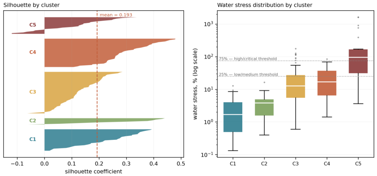
Figure 7.
Comparative performance of the six learners. Note. Left and centre: R² and RMSE under the random hold-out (light bars) and under grouped cross-validation with countries held out (dark bars). Right: out-of-fold predictions of the Random Forest against observed values, with the 45-degree line.
Figure 7.
Comparative performance of the six learners. Note. Left and centre: R² and RMSE under the random hold-out (light bars) and under grouped cross-validation with countries held out (dark bars). Right: out-of-fold predictions of the Random Forest against observed values, with the 45-degree line.
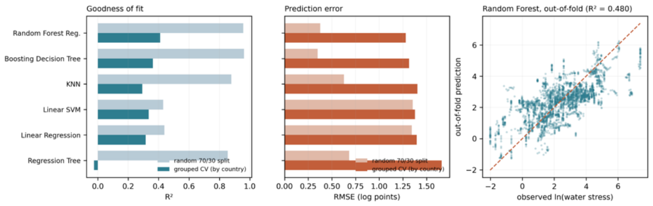
Figure 8.
Dropout loss for the Random Forest. Note. Bars report the increase in out-of-fold mean squared error when each variable is randomly permuted, expressed as a percentage of the baseline error.
Figure 8.
Dropout loss for the Random Forest. Note. Bars report the increase in out-of-fold mean squared error when each variable is randomly permuted, expressed as a percentage of the baseline error.
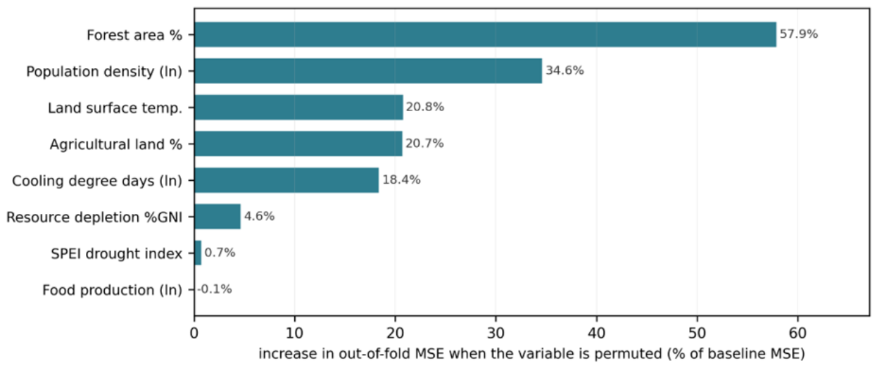
Figure 9.
SHAP additive explanations for the Random Forest. Note. Each point is one observation; horizontal position gives the contribution of that variable to the predicted log water stress, and colour encodes the value of the variable itself.
Figure 9.
SHAP additive explanations for the Random Forest. Note. Each point is one observation; horizontal position gives the contribution of that variable to the predicted log water stress, and colour encodes the value of the variable itself.
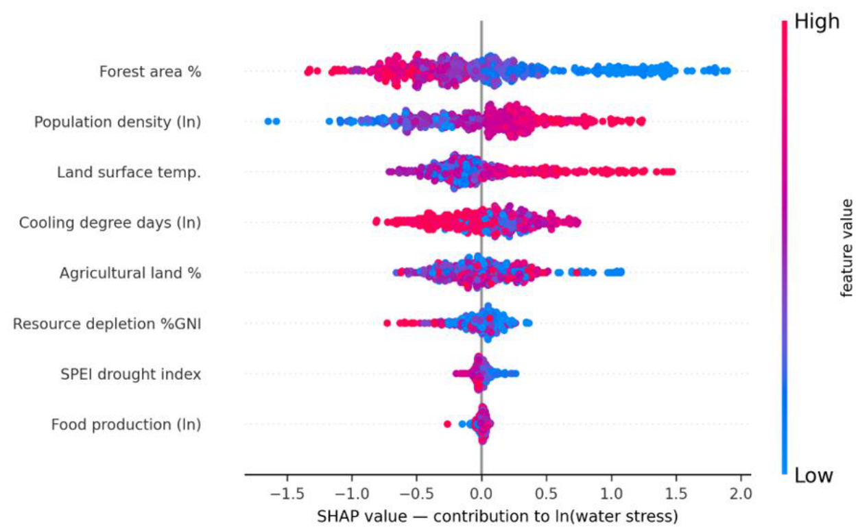
Figure 10.
Partial dependence of predicted log water stress on the four most important variables by dropout loss. Note. Tick marks along the horizontal axis show the distribution of the observed data.
Figure 10.
Partial dependence of predicted log water stress on the four most important variables by dropout loss. Note. Tick marks along the horizontal axis show the distribution of the observed data.
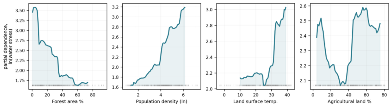
Figure 11.
Fixed-effects and Between coefficients on the social block with 95% confidence intervals. Note. Left: variables measured in percentage points. Right: demographic and health variables. The systematic sign reversal between the two estimators is the central result of the equation.
Figure 11.
Fixed-effects and Between coefficients on the social block with 95% confidence intervals. Note. Left: variables measured in percentage points. Right: demographic and health variables. The systematic sign reversal between the two estimators is the central result of the equation.
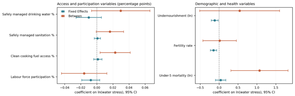
Figure 12.
Comparative performance of six clustering algorithms on the social block. Note. Cell values are the raw statistics; colour encodes the min–max normalised score, so that green marks the best-performing algorithm on each index.
Figure 12.
Comparative performance of six clustering algorithms on the social block. Note. Cell values are the raw statistics; colour encodes the min–max normalised score, so that green marks the best-performing algorithm on each index.
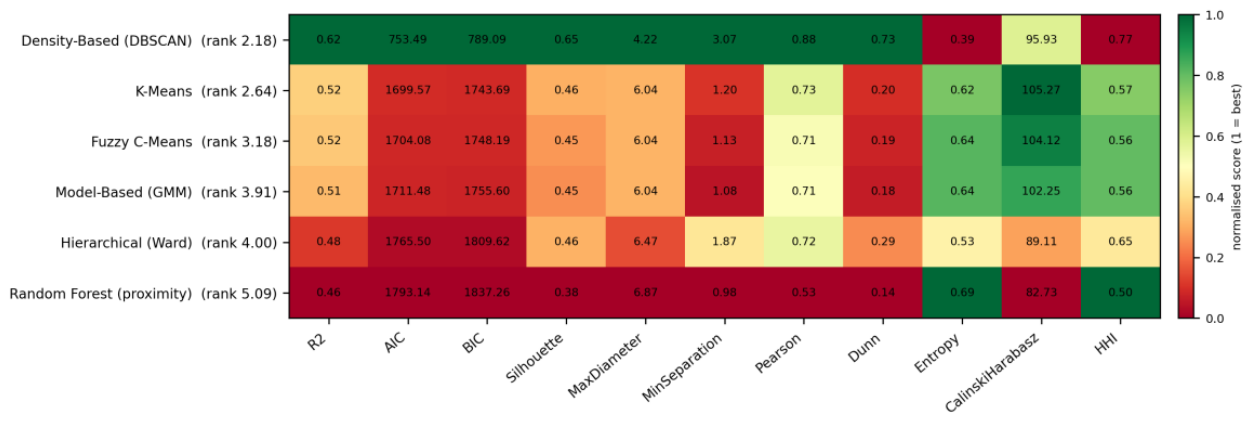
Figure 13.
Selection of the number of clusters for K-Means on the social block. Note. The silhouette optimum at k = 2 is visible in the centre panel; the elbow in the within-cluster sum of squares and the substantive separation of the high-stress group support k = 4 (dashed line).
Figure 13.
Selection of the number of clusters for K-Means on the social block. Note. The silhouette optimum at k = 2 is visible in the centre panel; the elbow in the within-cluster sum of squares and the substantive separation of the high-stress group support k = 4 (dashed line).
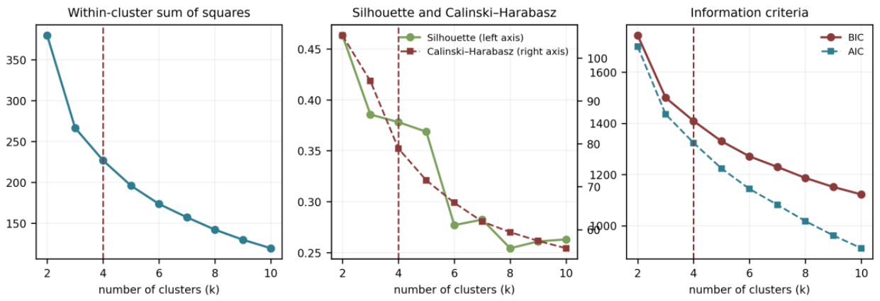
Figure 14.
K-Means partition of the social block in the space of the first two principal components, which jointly account for 82.1% of total variance. Note. Ellipses mark one and two standard deviations around each cluster centroid; arrows are the variable loadings.
Figure 14.
K-Means partition of the social block in the space of the first two principal components, which jointly account for 82.1% of total variance. Note. Ellipses mark one and two standard deviations around each cluster centroid; arrows are the variable loadings.
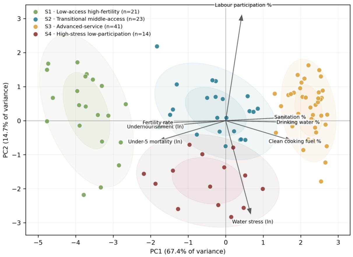
Figure 15.
Social profile of the four clusters. Note. Cell values are cluster means expressed in standard deviations from the global mean, so that red marks values above and blue values below the cross-country average.
Figure 15.
Social profile of the four clusters. Note. Cell values are cluster means expressed in standard deviations from the global mean, so that red marks values above and blue values below the cross-country average.
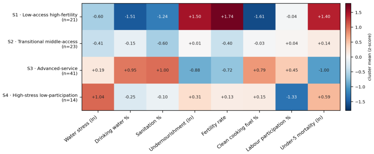
Figure 16.
Internal validity and outcome separation of the social partition. Note. Left: silhouette coefficients by cluster, with the overall mean marked. Right: the distribution of water stress by cluster on a logarithmic scale, against the conventional 25% and 75% thresholds.
Figure 16.
Internal validity and outcome separation of the social partition. Note. Left: silhouette coefficients by cluster, with the overall mean marked. Right: the distribution of water stress by cluster on a logarithmic scale, against the conventional 25% and 75% thresholds.
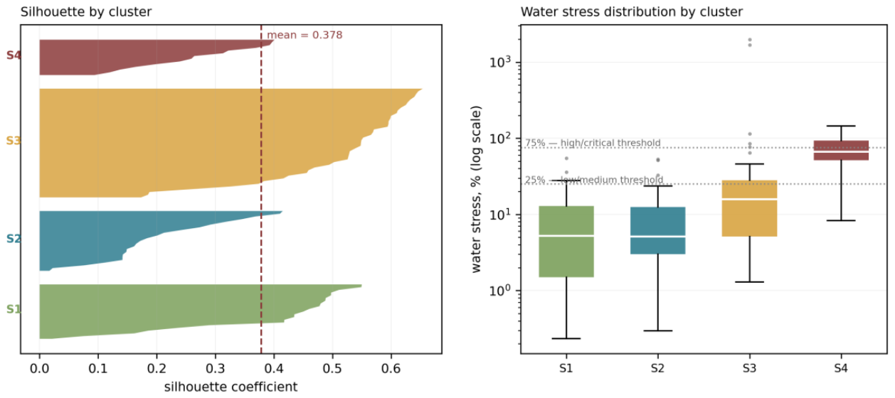
Figure 17.
Comparative performance of the six learners on the social block. Note. Left and centre: R² and RMSE under the random hold-out (light bars) and under grouped cross-validation (dark bars); three learners return negative R² in the grouped scheme. Right: out-of-fold predictions of the Random Forest against observed values, with the 45-degree line.
Figure 17.
Comparative performance of the six learners on the social block. Note. Left and centre: R² and RMSE under the random hold-out (light bars) and under grouped cross-validation (dark bars); three learners return negative R² in the grouped scheme. Right: out-of-fold predictions of the Random Forest against observed values, with the 45-degree line.
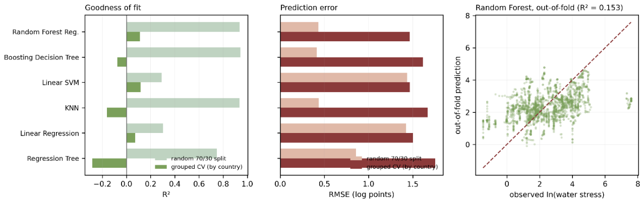
Figure 18.
Dropout loss for the Random Forest on the social block. Note. Bars report the increase in out-of-fold mean squared error when each variable is randomly permuted, as a percentage of the baseline error. The magnitudes are roughly half those obtained on the environmental block.
Figure 18.
Dropout loss for the Random Forest on the social block. Note. Bars report the increase in out-of-fold mean squared error when each variable is randomly permuted, as a percentage of the baseline error. The magnitudes are roughly half those obtained on the environmental block.
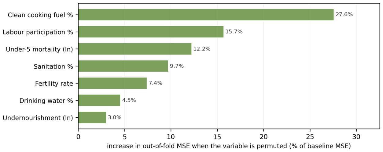
Figure 19.
SHAP additive explanations for the Random Forest on the social block. Note. Each point is one observation; horizontal position gives the contribution of that variable to predicted log water stress, and colour encodes the value of the variable.
Figure 19.
SHAP additive explanations for the Random Forest on the social block. Note. Each point is one observation; horizontal position gives the contribution of that variable to predicted log water stress, and colour encodes the value of the variable.
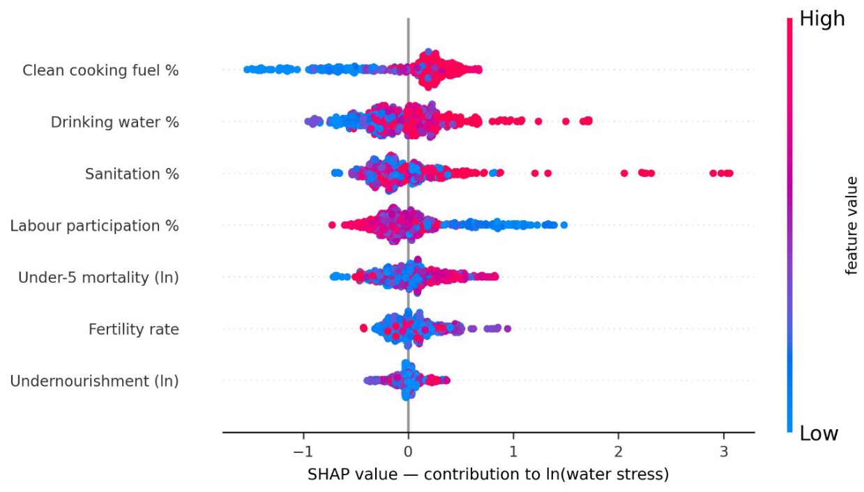
Figure 20.
Partial dependence of predicted log water stress on the four most important social variables by dropout loss. Note. Tick marks along the horizontal axis show the distribution of the observed data.
Figure 20.
Partial dependence of predicted log water stress on the four most important social variables by dropout loss. Note. Tick marks along the horizontal axis show the distribution of the observed data.
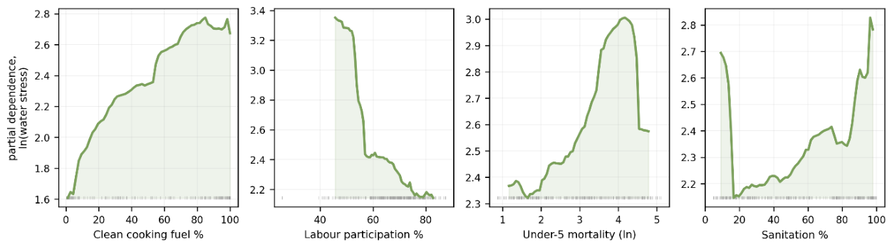
Figure 21.
Fixed-effects and Between coefficients on the governance block with 95% confidence intervals. Note. Left: the four Worldwide Governance Indicators. Right: economic environment, gender and innovation variables. The width of the Between intervals on the WGI dimensions, set against the narrowness of the fixed-effects intervals, is the first visible symptom of the collinearity problem.
Figure 21.
Fixed-effects and Between coefficients on the governance block with 95% confidence intervals. Note. Left: the four Worldwide Governance Indicators. Right: economic environment, gender and innovation variables. The width of the Between intervals on the WGI dimensions, set against the narrowness of the fixed-effects intervals, is the first visible symptom of the collinearity problem.
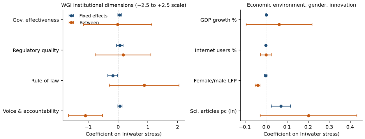
Figure 22.
Left: correlation matrix of the four WGI dimensions in the estimation sample. Note. Centre: scree plot of the principal components of the standardised matrix. Right: loadings of the first two components.
Figure 22.
Left: correlation matrix of the four WGI dimensions in the estimation sample. Note. Centre: scree plot of the principal components of the standardised matrix. Right: loadings of the first two components.
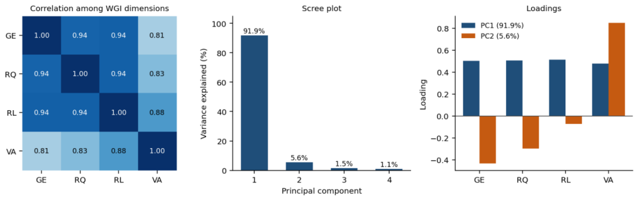
Figure 23.
Coefficients on each WGI dimension when entered singly and when entered jointly, with 95% confidence intervals, under fixed effects (left) and the Between estimator (right).
Figure 23.
Coefficients on each WGI dimension when entered singly and when entered jointly, with 95% confidence intervals, under fixed effects (left) and the Between estimator (right).
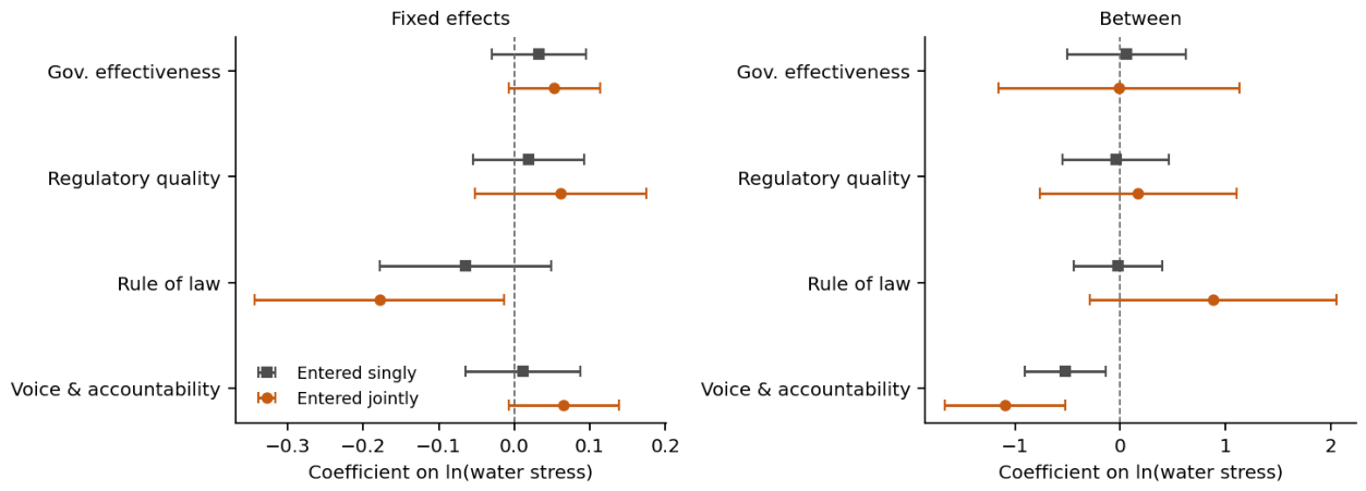
Figure 24.
Country means of log water stress against the two principal components. Note. Left: institutional quality. Right: institutional balance, with the six lowest-scoring economies labelled.
Figure 24.
Country means of log water stress against the two principal components. Note. Left: institutional quality. Right: institutional balance, with the six lowest-scoring economies labelled.
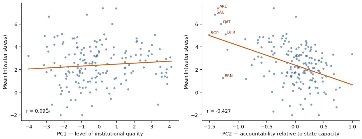
Figure 25.
Comparative performance of six clustering algorithms on the governance block. Note. Cell values are the raw statistics; colour encodes the min–max normalised score, so that green marks the best-performing algorithm on each index.
Figure 25.
Comparative performance of six clustering algorithms on the governance block. Note. Cell values are the raw statistics; colour encodes the min–max normalised score, so that green marks the best-performing algorithm on each index.
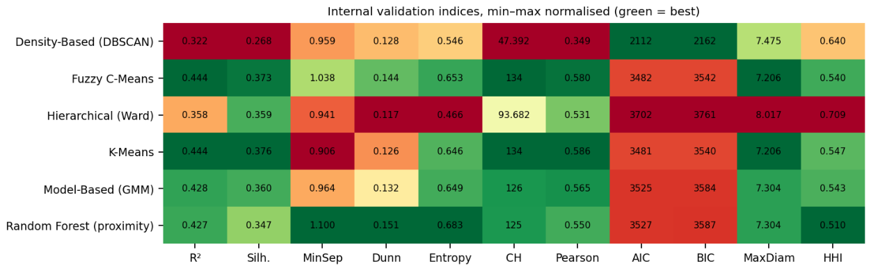
Figure 26.
Selection of the number of clusters for Fuzzy C-Means on the governance block. Note. The silhouette optimum at k = 2 is visible in the second panel; the elbow in the within-cluster sum of squares and the substantive separation of the high-stress group support k = 4 (dashed line). The partition coefficient in the fourth panel falls monotonically, from 0.706 at k = 2 to 0.433 at k = 4, confirming that the fuzziness of the solution rises steadily with k.
Figure 26.
Selection of the number of clusters for Fuzzy C-Means on the governance block. Note. The silhouette optimum at k = 2 is visible in the second panel; the elbow in the within-cluster sum of squares and the substantive separation of the high-stress group support k = 4 (dashed line). The partition coefficient in the fourth panel falls monotonically, from 0.706 at k = 2 to 0.433 at k = 4, confirming that the fuzziness of the solution rises steadily with k.
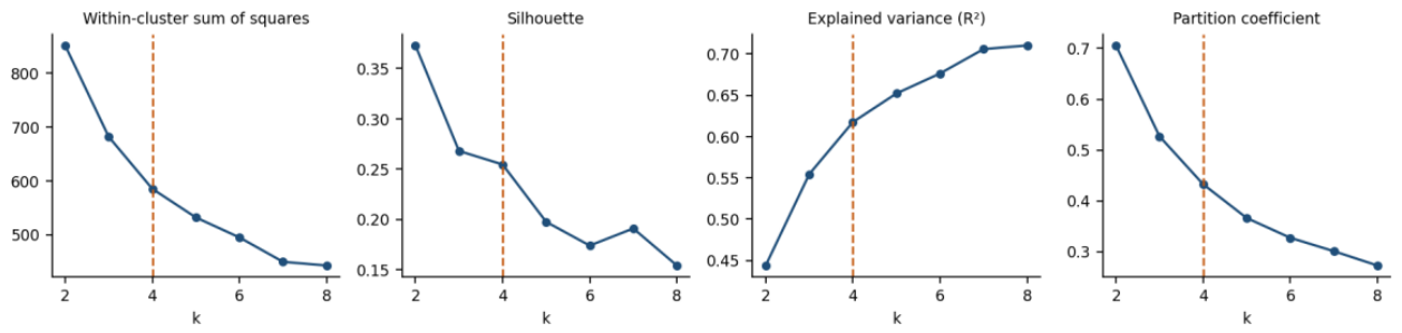
Figure 27.
Fuzzy C-Means partition of the governance block in the space of the first two principal components, which jointly account for 79.0% of total variance. Note. Ellipses mark one and two standard deviations around each cluster centroid; arrows are the variable loadings.
Figure 27.
Fuzzy C-Means partition of the governance block in the space of the first two principal components, which jointly account for 79.0% of total variance. Note. Ellipses mark one and two standard deviations around each cluster centroid; arrows are the variable loadings.
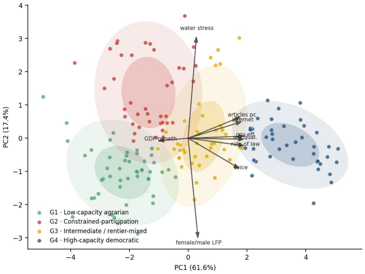
Figure 28.
Governance profile of the four clusters. Note. Cell values are cluster means expressed in standard deviations from the global mean, so that red marks values above and blue values below the cross-country average.
Figure 28.
Governance profile of the four clusters. Note. Cell values are cluster means expressed in standard deviations from the global mean, so that red marks values above and blue values below the cross-country average.
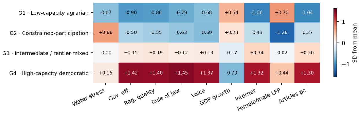
Figure 29.
Internal validity, membership strength and outcome separation of the governance partition. Note. Left: silhouette coefficients by cluster, with the overall mean marked. Centre: maximum membership degrees by cluster, with the 0.5 majority threshold. Right: the distribution of water stress by cluster on a logarithmic scale, against the conventional 25% and 75% thresholds.
Figure 29.
Internal validity, membership strength and outcome separation of the governance partition. Note. Left: silhouette coefficients by cluster, with the overall mean marked. Centre: maximum membership degrees by cluster, with the 0.5 majority threshold. Right: the distribution of water stress by cluster on a logarithmic scale, against the conventional 25% and 75% thresholds.
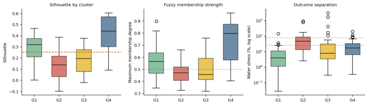
Figure 30.
Comparative performance of the six learners on the governance block. Note. Left and centre: R² and RMSE under the random hold-out (light bars) and under grouped cross-validation with countries held out (dark bars). Right: out-of-fold predictions of the Random Forest against observed values, with the 45-degree line.
Figure 30.
Comparative performance of the six learners on the governance block. Note. Left and centre: R² and RMSE under the random hold-out (light bars) and under grouped cross-validation with countries held out (dark bars). Right: out-of-fold predictions of the Random Forest against observed values, with the 45-degree line.
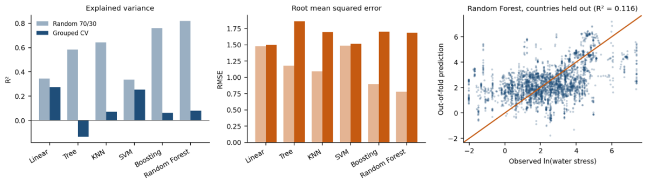
Figure 31.
Dropout loss for the Random Forest. Note. Bars report the increase in out-of-fold mean squared error when each variable is randomly permuted, expressed as a percentage of the baseline error. Note. Left: natural block. Right: orthogonalised block.
Figure 31.
Dropout loss for the Random Forest. Note. Bars report the increase in out-of-fold mean squared error when each variable is randomly permuted, expressed as a percentage of the baseline error. Note. Left: natural block. Right: orthogonalised block.
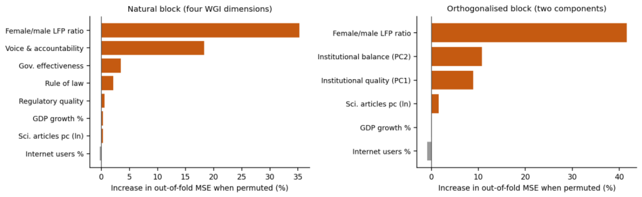
Figure 32.
SHAP additive explanations for the Random Forest on the natural block. Note. Each point is one observation; horizontal position gives the contribution of that variable to the predicted log water stress, and colour encodes the value of the variable itself.
Figure 32.
SHAP additive explanations for the Random Forest on the natural block. Note. Each point is one observation; horizontal position gives the contribution of that variable to the predicted log water stress, and colour encodes the value of the variable itself.
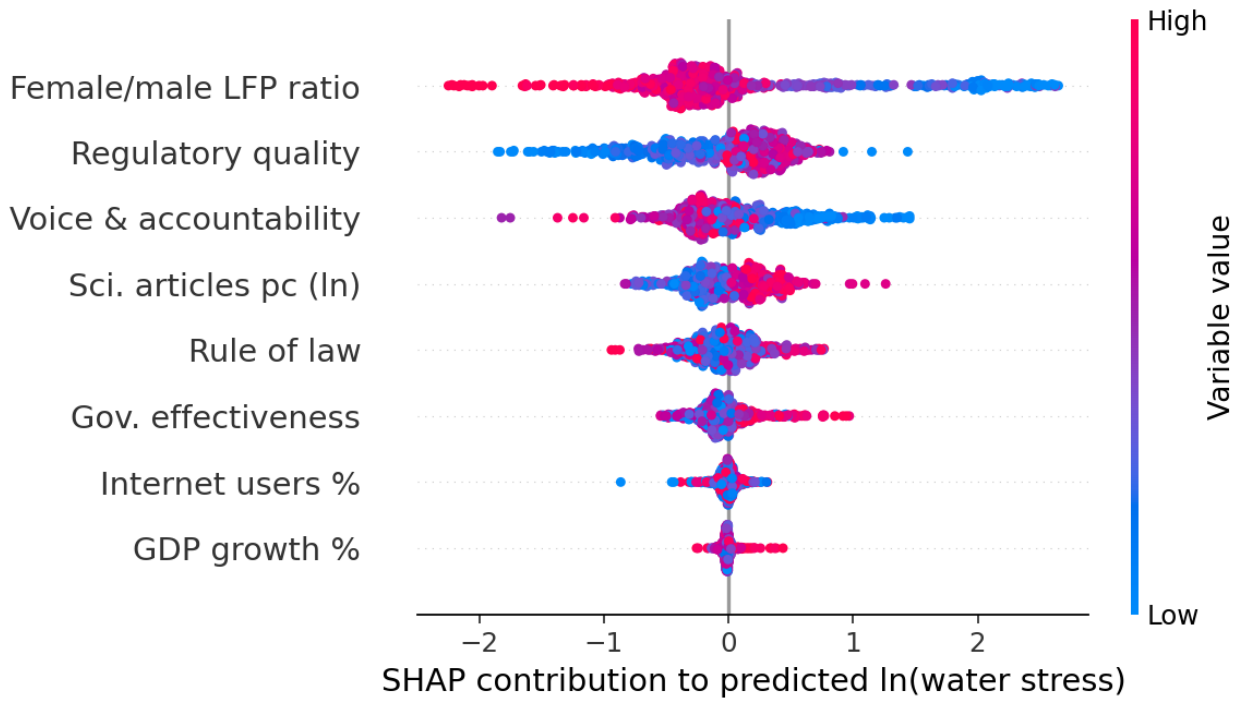
Figure 33.
Partial dependence of predicted log water stress on the four variables with the highest dropout loss. Note. Tick marks along the horizontal axis show the distribution of the observed data.
Figure 33.
Partial dependence of predicted log water stress on the four variables with the highest dropout loss. Note. Tick marks along the horizontal axis show the distribution of the observed data.
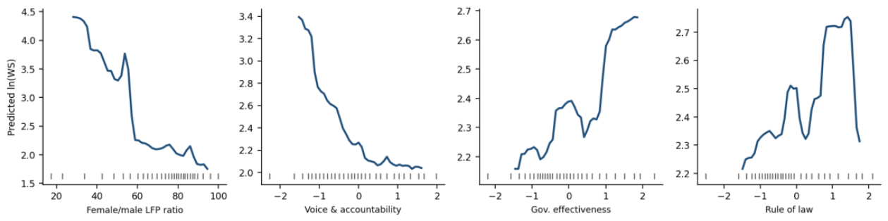
Table 1.
Environmental determinants of water stress: panel estimates, 2000–2021.
| Pooled OLS | Fixed Effects | Random Effects | Between | WLS | Diff-GMM (AB) | Sys-GMM (BB) | |
|---|---|---|---|---|---|---|---|
| L1.lnWS | — | — | — | — | — | 0.8436*** (0.1906) | 0.9482*** (0.0955) |
| lnFOOD | −0.0183 (0.2776) | −0.0710 (0.0810) | −0.0832 (0.0768) | 0.3379 (0.9970) | 0.4845 (0.4792) | 0.0151 (0.0314) | −0.0430* (0.0253) |
| AGRI | −0.0198*** (0.0061) | 0.0079* (0.0043) | 0.0062 (0.0041) | −0.0152*** (0.0056) | −0.0141 (0.0109) | 0.0043** (0.0020) | −0.0011 (0.0021) |
| FRST | −0.0458*** (0.0058) | −0.0042 (0.0105) | −0.0131 (0.0081) | −0.0360*** (0.0067) | −0.0448*** (0.0107) | −0.0027 (0.0036) | −0.0023 (0.0041) |
| SPEI | −0.0927*** (0.0338) | 0.0036 (0.0046) | 0.0052 (0.0045) | −1.0447*** (0.3066) | −0.2433*** (0.0834) | −0.0030 (0.0022) | −0.0026 (0.0042) |
| lnCDD | −0.1724 (0.1647) | −0.0181 (0.0336) | −0.0141 (0.0317) | −0.1805 (0.1775) | −0.0575 (0.3279) | 0.0146 (0.0169) | −0.0042 (0.0258) |
| LSTM | 0.0308 (0.0269) | −0.0093** (0.0043) | −0.0051 (0.0040) | 0.0319 (0.0303) | 0.0303 (0.0439) | −0.0034 (0.0033) | 0.0007 (0.0030) |
| lnDNST | 0.3965*** (0.0915) | 0.3420*** (0.1324) | 0.3293*** (0.1123) | 0.4302*** (0.0839) | 0.4351** (0.1948) | −0.0691 (0.0758) | 0.0238 (0.0447) |
| DRES | −0.0088 (0.0155) | −0.0012 (0.0013) | −0.0012 (0.0013) | −0.0099 (0.0173) | 0.0238 (0.0289) | 0.0005 (0.0011) | −0.0007 (0.0015) |
| Constant | 3.5828*** (1.3291) | 1.4781** (0.6902) | 1.7985*** (0.6025) | 1.0861 (4.5934) | −0.1382 (2.2271) | — | 0.3460 (0.4455) |
| N | 3,501 | 3,501 | 3,501 | 170 groups | 3,501 | 2,448 | 2,448 |
| R² | 0.4540 | 0.0654 (within) | 0.0761 | 0.4746 | 0.3770 | — | — |
Note. *** p<0.01, ** p<0.05, * p<0.10. Country-clustered standard errors in parentheses. GMM estimates are two-step with Windmeijer correction and collapsed instruments, gmm(lnWS, 2:4), on a balanced sub-panel of 136 countries over 18 years.
Table 2.
Internal validation indices, six algorithms at their own optimal configuration.
| Algorithm | k | n | R² | AIC | BIC | Sil. | MaxD | MinS | Pear. | Dunn | Ent. | CH | HHI |
|---|---|---|---|---|---|---|---|---|---|---|---|---|---|
| Density-Based (DBSCAN) | 2 | 120 | 0.117 | 2527.5 | 2580.5 | 0.384 | 6.540 | 2.719 | 0.477 | 0.416 | 0.146 | 15.60 | 0.936 |
| Fuzzy C-Means | 3 | 170 | 0.322 | 3804.2 | 3892.0 | 0.199 | 7.763 | 1.006 | 0.349 | 0.130 | 1.085 | 39.59 | 0.343 |
| Hierarchical (Ward) | 4 | 170 | 0.372 | 3704.8 | 3820.9 | 0.188 | 7.763 | 1.254 | 0.445 | 0.162 | 1.096 | 32.74 | 0.393 |
| K-Means | 7 | 170 | 0.557 | 3223.0 | 3423.7 | 0.201 | 6.825 | 0.955 | 0.450 | 0.140 | 1.836 | 34.21 | 0.173 |
| Model-Based (GMM) | 5 | 170 | 0.451 | 3516.5 | 3660.8 | 0.187 | 7.028 | 0.729 | 0.427 | 0.104 | 1.480 | 33.88 | 0.242 |
| Random Forest (proximity) | 4 | 170 | 0.322 | 3820.2 | 3936.2 | 0.165 | 7.613 | 1.017 | 0.349 | 0.134 | 1.159 | 26.34 | 0.328 |
Note. n = economies classified; Sil. = silhouette; MaxD = maximum within-cluster diameter; MinS = minimum between-cluster separation; Pear. = Pearson gamma; Ent. = entropy of cluster sizes; HHI = Herfindahl–Hirschman index of cluster size concentration. Higher is better for R², Sil., MinS, Pear., Dunn, Ent. and CH; lower is better for AIC, BIC, MaxD and HHI. DBSCAN classifies only 120 of the 170 economies, assigning the remaining 50 to noise.
Table 3.
Rank matrix across all eleven indices (1 = best).
| Algorithm | R² | Sil. | MinSep | Dunn | Entropy | CH | Pearson | AIC | BIC | MaxDiam | HHI | Mean rank |
|---|---|---|---|---|---|---|---|---|---|---|---|---|
| K-Means | 1 | 2 | 5 | 3 | 1 | 2 | 2 | 2 | 2 | 2 | 1 | 2.09 |
| Density-Based (DBSCAN) | 6 | 1 | 1 | 1 | 6 | 6 | 1 | 1 | 1 | 1 | 6 | 2.82 |
| Model-Based (GMM) | 2 | 5 | 6 | 6 | 2 | 3 | 4 | 3 | 3 | 3 | 2 | 3.55 |
| Hierarchical (Ward) | 3 | 4 | 2 | 2 | 4 | 4 | 3 | 4 | 4 | 5.5 | 5 | 3.68 |
| Fuzzy C-Means | 5 | 3 | 4 | 5 | 5 | 1 | 6 | 5 | 5 | 5.5 | 4 | 4.41 |
| Random Forest (proximity) | 4 | 6 | 3 | 4 | 3 | 5 | 5 | 6 | 6 | 4 | 3 | 4.45 |
Note. Ranks run from 1 (best) to 6 across the eleven indices of Table 2, with ties averaged. The mean rank is the unweighted average. DBSCAN scores highly on compactness only because it leaves fifty economies unclassified.
Table 4.
Cluster profiles, original units (period means 2000–2021).
| Cluster | n | Water stress % | Forest % | Agri. land % | SPEI | Cooling degree days | Land surf. temp. °C | Density | Resource depletion %GNI |
|---|---|---|---|---|---|---|---|---|---|
| C1 · Humid forested extractive | 32 | 1.5 | 63.1 | 22.1 | −0.07 | 4104 | 27.6 | 30 | 9.53 |
| C2 · Boreal water-abundant | 10 | 3.1 | 48.2 | 16.3 | +0.13 | 57 | 4.9 | 14 | 2.07 |
| C3 · Tropical agrarian dense | 61 | 13.0 | 24.7 | 50.6 | −0.22 | 3795 | 31.0 | 103 | 3.45 |
| C4 · Temperate industrialised | 42 | 14.7 | 29.8 | 47.1 | −0.30 | 335 | 16.4 | 108 | 0.68 |
| C5 · Arid extractive critical | 25 | 81.6 | 6.1 | 36.0 | −0.95 | 3661 | 34.4 | 33 | 11.45 |
Note. Water stress is the back-transformed cluster mean of the logged dependent variable. SPEI is the standardised precipitation–evapotranspiration index; density is people per square kilometre; resource depletion is adjusted savings as a share of gross national income.
Table 5.
Full cluster membership.
| Cluster | Member economies (ISO-3) |
|---|---|
| C1 · Humid forested extractive (n = 32) | AGO, BLZ, BOL, BRA, BRN, CAF, CMR, COD, COG, COL, DMA, ECU, FJI, GAB, GNB, GNQ, GUY, KHM, LAO, LBR, MMR, MYS, PAN, PER, PNG, PRY, SLE, SUR, TZA, VCT, VEN, ZMB |
| C2 · Boreal water-abundant (n = 10) | BTN, CAN, EST, FIN, ISL, LVA, NOR, NZL, RUS, SWE |
| C3 · Tropical agrarian dense (n = 61) | AFG, ARG, AUS, BDI, BEN, BFA, BGD, BRB, BWA, CIV, COM, CPV, CRI, CUB, CYP, DJI, DOM, ERI, ETH, GHA, GIN, GMB, GTM, HND, HTI, IDN, IND, ISR, JAM, KEN, LBN, LCA, LKA, MDG, MEX, MOZ, MUS, MWI, NAM, NGA, NIC, PAK, PHL, RWA, SDN, SEN, SGP, SLV, SOM, SSD, STP, SWZ, SYR, TGO, THA, TTO, UGA, URY, VNM, ZAF, ZWE |
| C4 · Temperate industrialised (n = 42) | ALB, ARM, AUT, BEL, BGR, BIH, BLR, CHE, CHL, CHN, CZE, DEU, DNK, ESP, FRA, GBR, GEO, GRC, HRV, HUN, IRL, ITA, JPN, KGZ, KOR, LSO, LTU, LUX, MDA, MKD, NLD, NPL, POL, PRT, ROU, SRB, SVK, SVN, TJK, TUR, UKR, USA |
| C5 · Arid extractive critical (n = 25) | ARE, AZE, BHR, DZA, EGY, IRN, IRQ, JOR, KAZ, KWT, LBY, MAR, MLI, MNG, MRT, NER, OMN, QAT, SAU, TCD, TKM, TLS, TUN, UZB, YEM |
Table 6.
Predictive performance, random 70/30 hold-out.
| Model | MAE | MSE | RMSE | RMSLE | MAPE | R2 |
| Linear Regression | 1.0508 | 1.8069 | 1.3442 | 1.1258 | 196.76 | 0.4374 |
| Regression Tree | 0.4426 | 0.4671 | 0.6835 | 0.5686 | 65.89 | 0.8546 |
| KNN | 0.4125 | 0.3928 | 0.6268 | 0.5193 | 49.41 | 0.8777 |
| Linear SVM | 1.0417 | 1.8317 | 1.3534 | 1.1404 | 194.10 | 0.4297 |
| Boosting Decision Tree | 0.2425 | 0.1227 | 0.3502 | 0.2818 | 27.25 | 0.9618 |
| Random Forest Reg. | 0.2624 | 0.1419 | 0.3767 | 0.2995 | 30.01 | 0.9558 |
Note. Errors are computed on the log scale of the dependent variable, except RMSLE and MAPE, which follow back-transformation to water stress in per cent. The partition is random across country-year rows, so countries appear on both sides.
Table 7.
Predictive performance, grouped five-fold cross-validation with countries held out.
| Model | MAE | MSE | RMSE | RMSLE | MAPE | R² |
|---|---|---|---|---|---|---|
| Linear Regression | 1.0959 | 1.9613 | 1.3967 | 1.1699 | 212.64 | 0.3143 |
| Regression Tree | 1.2858 | 2.7816 | 1.6607 | 1.4230 | 519.80 | −0.0248 |
| KNN | 1.1291 | 1.9891 | 1.4041 | 1.1745 | 211.75 | 0.2923 |
| Linear SVM | 1.0916 | 1.9180 | 1.3785 | 1.1597 | 199.60 | 0.3343 |
| Boosting Decision Tree | 1.0486 | 1.7561 | 1.3164 | 1.1178 | 229.58 | 0.3622 |
| Random Forest Reg. | 1.0105 | 1.6520 | 1.2807 | 1.0833 | 190.51 | 0.4098 |
Note. Metrics follow Table 6. Each fold holds out entire countries, so no economy appears in both training and test sets. Values are averages across the five folds. A negative R² indicates prediction worse than the sample mean.
Table 8.
Composite ranking across the five error metrics and R², both validation schemes.
| Model | Random split | Grouped CV | Mean rank |
|---|---|---|---|
| Random Forest Reg. | 2.0 | 1.0 | 1.50 |
| Boosting Decision Tree | 1.0 | 2.3 | 1.65 |
| KNN | 3.0 | 4.8 | 3.90 |
| Linear SVM | 5.8 | 2.9 | 4.35 |
| Linear Regression | 5.2 | 4.0 | 4.60 |
| Regression Tree | 4.0 | 6.0 | 5.00 |
Table 9.
Convergence between econometric coefficients and machine-learning attributions.
| Variable | FE coef | Between coef | Dropout loss % | Mean |SHAP| | SHAP direction | Between sign | Agreement |
|---|---|---|---|---|---|---|---|
| Forest area % | −0.0042 | −0.0360*** | 57.89 | 0.5072 | − | − | yes |
| Population density (ln) | +0.3420*** | +0.4302*** | 34.61 | 0.3721 | + | + | yes |
| Land surface temp. | −0.0093** | +0.0319 | 20.76 | 0.2887 | + | + | yes |
| Agricultural land % | +0.0079* | −0.0152*** | 20.69 | 0.2170 | + | − | no |
| Cooling degree days (ln) | −0.0181 | −0.1805 | 18.37 | 0.2521 | − | − | yes |
| Resource depletion %GNI | −0.0012 | −0.0099 | 4.63 | 0.1100 | − | − | yes |
| SPEI drought index | +0.0036 | −1.0447*** | 0.71 | 0.0366 | − | − | yes |
| Food production (ln) | −0.0710 | +0.3379 | −0.05 | 0.0213 | + | + | yes |
Note. *** p < 0.01, ** p < 0.05, * p < 0.10. SHAP direction is the sign of the correlation between a variable’s value and its SHAP contribution. Agreement compares that sign with the sign of the Between estimator, which is the econometric specification most comparable to a cross-sectional learner.
Table 10.
Social determinants of water stress, main specification (S-B), 2001–2022.
| Pooled OLS | Fixed Effects | Random Effects | Between | WLS | Diff-GMM | Sys-GMM | |
|---|---|---|---|---|---|---|---|
| L1.lnWS | — | — | — | — | — | 0.7379*** (0.1478) | 1.0040*** (0.0524) |
| Drinking water % | 0.0229 (0.0153) | −0.0100 (0.0080) | −0.0092 (0.0079) | 0.0297 (0.0185) | 0.0003 (0.0141) | −0.0019 (0.0023) | 0.0001 (0.0013) |
| Sanitation % | 0.0146** (0.0072) | 0.0007 (0.0020) | 0.0009 (0.0020) | 0.0162* (0.0087) | 0.0273*** (0.0095) | −0.0008 (0.0007) | −0.0006 (0.0011) |
| Undernourishment (ln) | 0.2699 (0.2839) | −0.1158** (0.0463) | −0.1150** (0.0462) | 0.5436 (0.5399) | 0.3570 (0.4057) | −0.0290 (0.0324) | −0.0037 (0.0274) |
| Fertility rate | 0.0302 (0.1694) | −0.1471*** (0.0427) | −0.1479*** (0.0428) | 0.0147 (0.2260) | 0.0359 (0.1928) | −0.0168 (0.0182) | 0.0045 (0.0135) |
| Clean cooking fuel % | 0.0216*** (0.0064) | 0.0013 (0.0026) | 0.0017 (0.0026) | 0.0228** (0.0096) | 0.0177** (0.0078) | 0.0002 (0.0008) | −0.0000 (0.0012) |
| Labour participation % | −0.0165 (0.0117) | −0.0075 (0.0057) | −0.0075 (0.0055) | −0.0158 (0.0144) | −0.0452** (0.0217) | −0.0000 (0.0010) | 0.0001 (0.0014) |
| Under-5 mortality (ln) | 0.9511*** (0.3278) | 0.0409 (0.0702) | 0.0521 (0.0690) | 1.0691*** (0.3860) | 0.5408 (0.3376) | 0.0060 (0.0197) | −0.0034 (0.0447) |
| Constant | −3.5462 (2.3642) | 3.9566*** (0.8894) | 3.8165*** (0.8786) | −5.0320* (2.5905) | 0.2089 (2.3529) | — | 0.0156 (0.1930) |
| N | 2,113 | 2,113 | 2,113 | 99 groups | 2,113 | 1,906 | 1,906 |
| R² | 0.2759 | 0.1092 (within) | 0.1029 | 0.3034 | 0.3030 | — | — |
Note. *** p < 0.01, ** p < 0.05, * p < 0.10. Country-clustered standard errors in parentheses. Sample: 99 economies, 2,113 country-year observations. GMM estimates are two-step with Windmeijer correction and collapsed instruments, gmm(lnWS, 2:4), on 98 economies with at least twelve consecutive observations. Hansen tests return χ²(2) = 0.175 (p = 0.916) for difference GMM and χ²(3) = 1.307 (p = 0.728) for system GMM; AR(1) is rejected (p = 0.012 and 0.001) while AR(2) is not (p = 0.883 and 0.866).
Table 11.
Robustness: specification as originally proposed (S-A), with the poverty headcount.
| Pooled OLS | Fixed Effects | Random Effects | Between | WLS | |
|---|---|---|---|---|---|
| Drinking water % | 0.0265* (0.0160) | −0.0200 (0.0157) | −0.0167 (0.0142) | 0.0320** (0.0156) | −0.0068 (0.0183) |
| Sanitation % | 0.0104 (0.0075) | 0.0021 (0.0030) | 0.0025 (0.0029) | 0.0140* (0.0082) | 0.0317*** (0.0087) |
| Undernourishment (ln) | 0.3853 (0.3634) | −0.2463*** (0.0641) | −0.2497*** (0.0632) | 0.6577 (0.5004) | −0.0795 (0.3997) |
| Fertility rate | 0.0456 (0.2278) | −0.2218*** (0.0720) | −0.2400*** (0.0703) | −0.2400 (0.2164) | 0.0969 (0.3738) |
| Poverty headcount (ln) | −0.2163 (0.1711) | −0.0598 (0.0445) | −0.0570 (0.0420) | −0.2763 (0.2302) | 0.1031 (0.2049) |
| Labour participation % | −0.0449*** (0.0151) | −0.0175* (0.0095) | −0.0175* (0.0092) | −0.0292* (0.0153) | −0.0859*** (0.0224) |
| Under-5 mortality (ln) | 0.5635* (0.3268) | 0.1125 (0.0813) | 0.1342* (0.0768) | 0.9853** (0.3778) | −0.2424 (0.3822) |
| Constant | 1.0595 (2.3003) | 5.7756*** (2.0125) | 5.3665*** (1.7565) | −1.3944 (2.3288) | 7.1816*** (2.4287) |
| N | 1,173 | 1,173 | 1,173 | 95 groups | 1,173 |
| R² | 0.1733 | 0.2376 (within) | 0.2369 | 0.2619 | 0.3635 |
Note. *** p < 0.01, ** p < 0.05, * p < 0.10. Country-clustered standard errors in parentheses. Sample: 95 economies, 1,173 country-year observations. The smaller sample reflects the irregular measurement of the poverty headcount.
Table 12.
Internal validation indices, six algorithms at their own optimal configuration.
| Algorithm | k | n | R² | AIC | BIC | Sil. | MaxD | MinS | Pear. | Dunn | Ent. | CH | HHI |
|---|---|---|---|---|---|---|---|---|---|---|---|---|---|
| Density-Based (DBSCAN) | 2 | 60 | 0.623 | 753.5 | 789.1 | 0.649 | 4.218 | 3.068 | 0.876 | 0.728 | 0.393 | 95.93 | 0.769 |
| Fuzzy C-Means | 2 | 99 | 0.518 | 1704.1 | 1748.2 | 0.453 | 6.039 | 1.126 | 0.712 | 0.187 | 0.637 | 104.12 | 0.556 |
| Hierarchical (Ward) | 2 | 99 | 0.479 | 1765.5 | 1809.6 | 0.465 | 6.473 | 1.870 | 0.724 | 0.289 | 0.530 | 89.11 | 0.654 |
| K-Means | 2 | 99 | 0.520 | 1699.6 | 1743.7 | 0.463 | 6.039 | 1.203 | 0.730 | 0.199 | 0.622 | 105.27 | 0.570 |
| Model-Based (GMM) | 2 | 99 | 0.513 | 1711.5 | 1755.6 | 0.449 | 6.039 | 1.075 | 0.706 | 0.178 | 0.637 | 102.25 | 0.556 |
| Random Forest (proximity) | 2 | 99 | 0.460 | 1793.1 | 1837.3 | 0.382 | 6.871 | 0.982 | 0.534 | 0.143 | 0.691 | 82.73 | 0.503 |
Note. n = economies classified; Sil. = silhouette; MaxD = maximum within-cluster diameter; MinS = minimum between-cluster separation; Pear. = Pearson gamma; Ent. = entropy of cluster sizes; CH = Calinski–Harabasz; HHI = Herfindahl–Hirschman index of cluster size concentration. Higher is better for R², Sil., MinS, Pear., Dunn, Ent. and CH; lower is better for AIC, BIC, MaxD and HHI.
Table 14.
Cluster profiles, original units (period means 2001–2022).
| Cluster | n | Water stress % | Drinking water % | Sanitation % | Undernour. % | Fertility | Clean fuel % | Labour part. % | Under-5 mortality |
|---|---|---|---|---|---|---|---|---|---|
| S1 · Low-access high-fertility | 21 | 4.17 | 18.2 | 17.0 | 19.70 | 5.21 | 8.1 | 66.9 | 85.5 |
| S2 · Transitional middle-access | 23 | 5.71 | 60.4 | 36.5 | 5.95 | 2.08 | 68.7 | 67.7 | 19.5 |
| S3 · Advanced-service | 41 | 14.97 | 94.8 | 85.2 | 2.64 | 1.61 | 99.7 | 72.2 | 5.1 |
| S4 · High-stress low-participation | 14 | 59.19 | 57.3 | 51.6 | 7.67 | 2.85 | 75.5 | 53.0 | 33.0 |
Note. Water stress, undernourishment and under-five mortality are back-transformed cluster means of the corresponding logged variables. Under-five mortality is per 1,000 live births; fertility is births per woman; the remaining variables are percentages.
Table 17.
Predictive performance, random 70/30 hold-out.
| Model | MAE | MSE | RMSE | RMSLE | MAPE | R² |
|---|---|---|---|---|---|---|
| Linear Regression | 1.1153 | 2.0302 | 1.4249 | 1.2188 | 226.72 | 0.3023 |
| Regression Tree | 0.5782 | 0.7337 | 0.8566 | 0.7309 | 77.17 | 0.7478 |
| KNN | 0.1558 | 0.1905 | 0.4364 | 0.3740 | 14.93 | 0.9345 |
| Linear SVM | 1.0960 | 2.0611 | 1.4356 | 1.2310 | 226.33 | 0.2917 |
| Boosting Decision Tree | 0.2803 | 0.1714 | 0.4140 | 0.3526 | 31.32 | 0.9411 |
| Random Forest Reg. | 0.2964 | 0.1861 | 0.4314 | 0.3649 | 32.80 | 0.9360 |
Table 18.
Predictive performance, grouped five-fold cross-validation with countries held out.
| Model | MAE | MSE | RMSE | RMSLE | MAPE | R² |
|---|---|---|---|---|---|---|
| Linear Regression | 1.2322 | 2.3937 | 1.5029 | 1.2958 | 237.58 | 0.0710 |
| Regression Tree | 1.4083 | 3.1360 | 1.7540 | 1.5287 | 293.01 | −0.2828 |
| KNN | 1.3179 | 2.8514 | 1.6677 | 1.4427 | 281.56 | −0.1621 |
| Linear SVM | 1.1854 | 2.2765 | 1.4664 | 1.2541 | 238.75 | 0.1164 |
| Boosting Decision Tree | 1.2882 | 2.7112 | 1.6125 | 1.3952 | 248.57 | −0.0750 |
| Random Forest Reg. | 1.1863 | 2.2839 | 1.4651 | 1.2785 | 213.88 | 0.1122 |
Table 19.
Composite ranking across the five error metrics and R², both validation schemes.
| Model | Random split | Grouped CV | Mean rank |
|---|---|---|---|
| Random Forest Reg. | 2.2 | 1.8 | 2.00 |
| Boosting Decision Tree | 1.2 | 4.0 | 2.60 |
| Linear SVM | 5.8 | 1.3 | 3.55 |
| KNN | 2.6 | 5.0 | 3.80 |
| Linear Regression | 5.2 | 2.9 | 4.05 |
| Regression Tree | 4.0 | 6.0 | 5.00 |
Table 20.
Convergence between econometric coefficients and machine-learning attributions.
| Variable | FE coef | Between coef | Dropout loss % | Mean |SHAP| | SHAP direction | Between sign | Agreement |
|---|---|---|---|---|---|---|---|
| Clean cooking fuel % | +0.0013 | +0.0228** | 27.57 | 0.3638 | + | + | yes |
| Labour participation % | −0.0075 | −0.0158 | 15.67 | 0.2601 | − | − | yes |
| Under-5 mortality (ln) | +0.0409 | +1.0691*** | 12.21 | 0.2093 | + | + | yes |
| Sanitation % | +0.0007 | +0.0162* | 9.69 | 0.2705 | + | + | yes |
| Fertility rate | −0.1471*** | +0.0147 | 7.38 | 0.1592 | + | + | yes |
| Drinking water % | −0.0100 | +0.0297 | 4.52 | 0.2955 | + | + | yes |
| Undernourishment (ln) | −0.1158** | +0.5436 | 2.98 | 0.0793 | + | + | yes |
Note. *** p < 0.01, ** p < 0.05, * p < 0.10. SHAP direction is the sign of the correlation between a variable’s value and its SHAP contribution. Agreement compares that sign with the sign of the Between estimator.
Disclaimer/Publisher’s Note: The statements, opinions and data contained in all publications are solely those of the individual author(s) and contributor(s) and not of MDPI and/or the editor(s). MDPI and/or the editor(s) disclaim responsibility for any injury to people or property resulting from any ideas, methods, instructions or products referred to in the content. |
© 2026 by the authors. Licensee MDPI, Basel, Switzerland. This article is an open access article distributed under the terms and conditions of the Creative Commons Attribution (CC BY) license (http://creativecommons.org/licenses/by/4.0/).
Copyright: This open access article is published under a Creative Commons CC BY 4.0 license, which permit the free download, distribution, and reuse, provided that the author and preprint are cited in any reuse.