
Submitted:
24 August 2026
Posted:
25 August 2026
You are already at the latest version
Abstract
Smart-city platforms connect Internet of Things (IoT) devices across transport, energy, water, healthcare and e-government services, so every gateway is an entry point and every log shared evidence. This paper evaluates a four-layer architecture: edge intrusion detection trained across districts by federated learning, digests anchored on a permissioned ledger, and a cloud orchestrator that correlates and audits. Its contribution, LPRA, is an aggregation rule whose accept and quarantine decisions are recorded on that ledger. On 211,043 public IoT testbed flows with identifier-free metadata, a depth-8 tree reached F1 = 0.997 at 17.7 KB and a CPU-time-scaled estimate of 0.19 J per million flows. Federated learning across five heterogeneous districts reached 0.971 ± 0.001, against 0.952 ± 0.002 alone. Under four poisoning attacks and an adaptive attacker that knows the screen, LPRA matched the best robust baselines and, unlike them, did not reduce F1 against FedAvg without an attack; the sweep also located and repaired a failure at 40% collusion. Anchoring ran at 146 tx/s on a two-organisation Fabric network. Generalisation fails twice: F1 falls from 0.96 within a dataset to 0.12 across datasets, and from 0.9824 under a random split to 0.0005 on a later capture day. Training must stay local and continuous.
Keywords:
smart city
; cybersecurity
; Internet of Things
; intrusion detection
; edge computing
; federated learning
; model poisoning
; Byzantine-robust aggregation
; permissioned blockchain
; Hyperledger Fabric
; digital trust
; TON_IoT
1. Introduction
Cities are becoming cyber-physical systems. Traffic controllers, smart meters, water-quality sensors, hospital equipment and citizen-facing e-government portals are increasingly connected through IoT gateways, edge nodes and municipal clouds. The same connectivity that enables data-driven services also enlarges the attack surface: IoT devices are resource-constrained and rarely patched, city networks span many administrative domains, and security evidence (alerts, logs, model versions) is produced by different agencies that do not necessarily trust one another [1,2]. A ransomware or DDoS campaign that starts in one district can propagate to others before a central security operations centre notices, and once an incident is disputed—between a utility, the police and the municipality—the integrity of the logs themselves becomes the question.
The perimeter of each district is itself a policy-enforcement problem whose structure decides whether a filter’s verdicts can be audited at all and how fast it can run at cloud scale [3,4]; the traffic that passes that perimeter is increasingly carried by encrypted transports such as QUIC, whose security implications for IoT deployments have been studied separately [5] and which leave an auditor with flow metadata rather than payload; the detector that judges what the filter admits is therefore a compact learner over metadata, whose behaviour depends on design choices as fine-grained as its activation function [6]; and a ledger that records security evidence for a small, known and mutually accountable set of city agencies is closer to public-sector deployments such as a government lottery ledger [7] than to an open, token-driven network. Three technologies are frequently proposed to address parts of this problem. Machine-learning intrusion detection systems (IDS) flag anomalous flows at the network edge; federated learning (FL) lets districts improve a shared model without exporting raw traffic; and permissioned blockchains provide tamper-evident, multi-party audit trails. Each has been evaluated in isolation on public datasets, but a city operator cannot deploy them in isolation, and combining them raises questions that single-technology studies do not answer: how small an edge model can be before detection quality collapses; how much accuracy is sacrificed when districts refuse to share data; whether a shared model can be protected from a compromised district without silently excluding honest ones; how much latency and storage a ledger adds to every alert; and whether a model trained on one kind of traffic is of any use for another. Recent studies also warn that IDS models generalise poorly across datasets and that identifier features such as IP addresses inflate reported accuracy [8,9,10,11].
This paper addresses these questions with an integrated, reproducible evaluation. The contributions are:
- A four-layer trustworthy security architecture for smart-city IoT (edge AI, federated learning, permissioned ledger, cloud orchestration) with an explicit threat model that covers external attacks on city services and insider attacks on the security system itself (forged alerts, rogue nodes, model poisoning), and a table mapping every threat to the layer that mitigates it and the experiment that tests it.
- A ledger-anchored poisoning-resilient aggregation rule (LPRA) for the federated layer: client updates are screened with a two-stage robust distance and direction test before averaging, and the accept/quarantine decision plus the resulting model hash are written to the consortium ledger every round, giving all agencies an auditable provenance of the detection model. LPRA is benchmarked head-to-head against Median, Trimmed Mean, Krum and Multi-Krum with one and two attackers, including an adaptive stealth attack, and combined with a personalised fine-tuning step for strongly non-IID districts.
- A bias-aware, dataset-agnostic feature schema (identifiers removed; nine directional and four direction-free semantic flow features) that enables cross-dataset evaluation spanning IoT (TON_IoT) and enterprise (CIC-IDS2017, UNSW-NB15) traffic in a single smart-city framework, with perimeter-firewall logs treated in the supplement. The direction-free view is defined so that datasets without a directional split, such as CICIoT2023, can be added without changing the schema; that dataset is supported by the released loader but is not part of the evaluation reported here.
- A validity and scalability study that goes beyond random splits: leave-one-attack-family-out (unseen-attack) evaluation, feature-importance ablation, five-seed confidence intervals, scaling from 5 to 50 districts and 3 to 15 ledger validators, and a replayed city-wide zero-day ransomware scenario that reports time-to-detect per layer.
- Quantitative answers to three research questions—RQ1: which lightweight model gives the best detection/footprint trade-off at the edge; RQ2: what federated training costs relative to centralised training under realistic non-IID district data, measured as raw-data exposure and communication volume rather than as a formal privacy guarantee, and how that changes under model poisoning; RQ3: what throughput, latency and storage overhead a permissioned ledger adds for trust—together with an open-source pipeline in which every reported experimental table, figure and numerical result is regenerated from the released experiment output.
2. Related Work
2.1. Smart-City Security and IoT Datasets
Surveys of IoT in smart cities identify security, interoperability and governance as the main open challenges [1,2]. The primary benchmark used here is TON_IoT [12,13,14], whose network dataset was released for edge-based smart-city security [12] and whose heterogeneity and lack of feature standardisation have been analysed in depth [14]. A second IoT testbed, CICIoT2023 [15], covers 105 real devices and 33 attacks; it is supported by our loader but not evaluated here, for the reason given in Section 4.2. Municipal data-centre traffic is represented by CIC-IDS2017 [16] and UNSW-NB15 [17], and perimeter decisions by the Internet Firewall Data Set [18]. Further testbeds complete the picture: Edge-IIoTset [19], whose seven-layer edge/fog/cloud testbed already includes a Hyperledger Sawtooth layer, Bot-IoT [20], and the reproducible Gotham 2025 release [21]. Statistical-learning botnet detection for smart-city networks has been demonstrated on TON_IoT [22], and standardised NetFlow feature sets have been proposed so that models can be compared across datasets at all [23]—a concern our common and direction-free views share. Sommer and Paxson [8] and Ring et al. [9] caution that testbed artefacts and identifier features lead to optimistic results, Cantone et al. [10] show large cross-dataset performance drops, and Dharini et al. [11] recently proposed a bias-aware refinement of TON_IoT that removes IP and port identifiers and reaches 0.986 accuracy with a decision tree on five flow features; we adopt the same bias-aware principle and extend it to a multi-dataset schema. The perimeter that precedes the detector is a policy problem in its own right: an anomaly-free rule structure is what makes a filter’s decisions auditable, and the tree-rule design was introduced for exactly that purpose and shown to improve security in cloud networks [3] and to sustain high-speed transmission in hybrid form [4]. What the filter admits is another matter, and it is increasingly opaque: as IoT services migrate to QUIC and similar encrypted transports, payload inspection stops being an option and the residual security questions shift to the transport and to flow behaviour [5]. Our architecture assumes such a filter in front of each district gateway and asks what should happen to the traffic it admits, using metadata alone.
2.2. Edge and Federated Intrusion Detection
Lightweight IDS models for gateways (decision trees, small random forests, compact MLPs) have been evaluated on individual datasets, mostly reporting accuracy alone; deployment metrics such as per-flow latency, model size and false-positive rate are reported less often. Federated averaging [24] enables collaborative training without data sharing; its behaviour under non-IID client data is a known challenge and has motivated proximal and personalised variants [25,26]. Federated anomaly detection has been demonstrated for IoT device populations [27], but without an audit trail of which client contributed what. Byzantine-robust aggregation rules—Krum and Multi-Krum [28], coordinate-wise Median and Trimmed Mean [29]—protect against malicious clients, but adaptive attacks such as “a little is enough” [30] can stay inside the honest norm envelope, an attacker who knows the defence can craft updates specifically against it [31], and a backdoor can be embedded while aggregate accuracy is left intact [32]; robustness claims must therefore state the attack model they assume, and robust rules are in any case known to sacrifice accuracy on heterogeneous data. Defences answer this in different ways: FLTrust bootstraps a trusted direction from a small server-side dataset [33], and FLAME combines clustering, clipping and noise to neutralise backdoors [34]; LPRA instead keeps the aggregation rule simple enough that its verdict on each client can be written down, endorsed and appealed. The privacy of the updates themselves is a separate axis, addressed by secure aggregation [35] and bounded by what can be reconstructed from a gradient [36]. Few works place FL inside a complete city security workflow with auditable model provenance.
2.3. Blockchain for Security Auditing
Permissioned blockchains such as Hyperledger Fabric [37] provide membership services, endorsement policies and ordered, tamper-evident ledgers among known organisations, which matches the multi-agency structure of a city. Combinations of blockchain and federated learning have been proposed for on-device learning [38] and for privacy-preserved data sharing in industrial IoT [39], establishing the pattern of exchanging models while anchoring their provenance. Prior proposals store IDS alerts or model hashes on-chain, but rarely report the storage and latency overhead relative to a conventional database, or test whether the ledger actually detects insider tampering.
2.4. Research Gap
To our knowledge no prior study evaluates edge IDS, federated learning with poisoning-resilient and auditable aggregation, and a permissioned ledger together on public testbed traffic with a common bias-aware schema, quantifies the trade-offs between the layers, and reports time-to-detect for a multi-district campaign in a smart-city setting.
3. Threat Model and Proposed Architecture
3.1. System and Adversary Model
We consider a city composed of K districts (Transport, Energy, Water, Healthcare, e-Government), each operating an IoT network behind a district gateway, and a set of agencies (municipal IT, police, electric utility, water authority, university) that jointly govern security evidence. Three adversary classes are modelled (Table 1). External adversary A1 compromises IoT devices or attacks services with DDoS/DoS, scanning, injection, XSS, password, backdoor, ransomware and MITM traffic (the TON_IoT attack families). Insider adversary A2 controls one district gateway or one agency account and attempts (i) to alter or delete alerts after the fact, (ii) to inject alerts from an un-enrolled node, or (iii) to poison the shared detection model by sending scaled, noisy, label-flipped or adaptively disguised weight updates. Privacy adversary A3 is a curious cloud operator who must not receive raw traffic. Confidentiality of payloads and cryptographic key management are handled by TLS and the ledger’s membership service and are out of scope; a colluding majority of districts or agencies is outside the model.
3.2. Architecture
Figure 1 shows the four layers. L1 (IoT/network) produces flow records at each district gateway. L2 (edge AI) runs a lightweight IDS model on the gateway; every gateway also participates in federated training rounds coordinated by the cloud, sending only model weights. L3 (permissioned ledger) is a consortium blockchain whose validators are the city agencies; a block is committed under a Proof-of-Authority round-robin proposer when at least 2/3 + 1 validators sign the header (the lightweight consensus is deliberate: with a small, known and mutually accountable set of organisations, Proof-of-Authority buys availability and simplicity where PBFT [40] buys resilience to arbitrary faults [41], while public-sector ledgers designed for known, accountable participants, such as a government lottery [7], make the same trade in favour of accountability over open participation), and only principals on the channel’s enrolment list may submit transactions. Only digests are stored on-chain: an alert transaction contains the district, model identifier, timestamp and the SHA-256 hash of the evidence flow; a model-update transaction contains the round number, the SHA-256 hash of the aggregated weights, the accepted and quarantined district lists and the screening statistics. Raw flows and personal data remain in the district’s off-chain store. L4 (cloud orchestrator) ingests alerts, correlates them across districts to detect city-wide campaigns, runs the LPRA aggregator, and audits districts by recomputing Merkle proofs [42] of their locally stored alerts against block roots, so that any post-hoc modification is detected without trusting the district.
3.3. Design Rationale
The layers are complementary rather than redundant: a district’s packet filter decides what is allowed, an anomaly-free rule structure keeps that decision auditable [3,4], and L2 then judges the behaviour of the traffic that the filter admits. Placing detection at the edge bounds latency and keeps raw traffic local; anchoring only hashes on the ledger keeps on-chain volume small and avoids storing personal data in an immutable structure; anchoring model versions on the same ledger gives every district a verifiable provenance of the model it executes; and Merkle proofs allow the cloud to audit a single alert without downloading whole blocks.
3.4. Ledger-Anchored Poisoning-Resilient Aggregation (LPRA)
FedAvg trusts every district equally, so a single compromised gateway (A2-iii) can shift the global model by sending a scaled, noisy or label-flipped update. Classical robust rules (Median, Trimmed Mean, Krum) resist this but discard information from every client on every round, which is costly when districts are legitimately different. LPRA instead screens the K client weight vectors and averages those that pass. Let m be the coordinate-wise median of the client vectors, dᵢ the Euclidean distance from client i to that median, and MAD(d) the median absolute deviation of those distances. Stage 1 (magnitude) quarantines client i if dᵢ > max(median(d) + τ·MAD(d), γ·median(d)), with τ = 3 and γ = 2.5; the MAD term is a robust z-score—a mean/standard-deviation threshold is itself dragged by the outlier and fails with K = 5—and the γ floor prevents the test from firing on tiny spreads. Stage 2 (direction) computes the cosine cᵢ between the client’s delta (the client’s delta) and the coordinate-wise median delta of the stage-1 survivors, and quarantines client i if cᵢ < 0.2—the signature of an update that pushes against the crowd (label flipping). The rule as first formulated (v1) used the *mean* delta of the survivors here and imposed no majority requirement; Section 5.3 shows how an adaptive attacker exploits that, and every experiment in this paper other than the explicit v1/v2 comparison uses the median form (v2) of Algorithm 1. Accepted clients are averaged with sample-size weights. The aggregator then submits one MODEL_UPDATE transaction containing the round, the SHA-256 hash of the new global weights, the accepted and quarantined district lists and the screening statistics (distances, cosines and thresholds). Because the transaction is endorsed by the agency quorum, a district cannot be silently excluded and the cloud cannot silently substitute a model: every gateway verifies the hash of the model it downloads against the ledger before deployment, and an excluded district can appeal with the recorded statistics. After convergence each district optionally performs one epoch of local fine-tuning (personalised FL) to adapt to its own traffic mix; the personalised model is a local artefact and is not anchored.
Algorithm 1(LPRA aggregation, one round). Input: client weight vectors w1…w_K, sample counts n1…n_K, current global vector w_g (the global model of the previous round), and thresholds τ = 3, γ = 2.5 and c_min = 0.2. (1) m ← coordinate-wise median of {wᵢ}. (2) dᵢ ← ‖wᵢ − m‖2 for every i; MAD ← 1.4826 · median(|d − median(d)|). (3) θ ← max(median(d) + τ·MAD, γ·median(d)); S1 ← {i : dᵢ ≤ θ}; if S1 = ∅ then S1 ← {argmin d}. (4) r ← coordinate-wise median of the survivor deltas {wᵢ − w_g : i ∈ S1}. (5) cᵢ ← cos(wᵢ − w_g, r) for i ∈ S1, where cos(u, v) is defined as 1 when both vectors have zero norm and 0 when exactly one does; A ← {i ∈ S1 : cᵢ ≥ c_min}. (6) if |A| ≤ ⌊K/2⌋ and |S1| ≥ ⌊K/2⌋+1, then A ← the ⌊K/2⌋+1 clients of S1 with the largest cᵢ; if |S1| ≤ ⌊K/2⌋ the round is not aggregated: w_g is kept, the round is anchored as INCONCLUSIVE with the full statistics, and the operator is notified. A client rejected at stage 1 is never readmitted by this step. (7) w_g′ ← (Σ over i ∈ A of nᵢ wᵢ) ⁄ (Σ over i ∈ A of nᵢ). (8) submit MODEL_UPDATE{round, SHA-256(w_g′), A, {1…K}\A, (d, c, θ)} to the ledger. Steps (4)–(6) are the v2 rule; the v1 rule used the mean in (4) and omitted (6), and Section 5.3 shows what that costs. The inconclusive branch of (6) did not occur in any experiment reported here—it exists so that the rule is total, and because a screen that cannot say “I do not know” will eventually say something worse.
Cost. Each round is O(K·d) time and O(K·d) memory for K clients and d parameters: the median, the K distances and the K cosines are each linear in the number of parameters, so LPRA adds a constant factor to the FedAvg it replaces and nothing that grows with the training set. For the (32,16) network used here, d = 2,305 and K = 5, so the screen is microseconds of work against seconds of local training. The claim made in this paper is that LPRA does not lose accuracy when no attack is present, not that it is free: it always computes the statistics and always writes one ledger transaction per round.
Thresholds. τ = 3 is the conventional three-sigma point transposed to a robust scale, since MAD·1.4826 estimates the standard deviation of a Gaussian; γ = 2.5 is a floor that prevents the MAD term from firing when the honest spread is near zero, which happens with small K in early rounds; c_min = 0.2 admits any client whose update is not actively opposed to the reference, rather than requiring agreement. None of the three was tuned to the results reported here. Their sensitivity is measured rather than assumed: Supplementary Table S4 sweeps γ at the hardest heterogeneity we test (K = 20, extreme non-IID), and Section 5.3 sweeps the attacker’s position relative to θ across two orders of magnitude.
Relation to other defences. FLTrust [33] and FLAME [34] address the same threat with more machinery: FLTrust bootstraps a trusted direction from a clean root dataset held by the server, and FLAME combines clustering, norm clipping and noise. Neither is used as a baseline here, and the reason is the threat model rather than convenience. A city consortium has no party entitled to hold a clean root dataset—that is the assumption the architecture exists to avoid—and a defence whose verdict cannot be reduced to a few numbers cannot be written into a ledger transaction that an excluded district may contest. LPRA is deliberately the simplest rule whose decision is explainable, auditable and appealable; where those constraints do not apply, the more elaborate defences are likely to be stronger.
4. Materials and Methods
4.1. Datasets
Three public datasets are evaluated here (Table 2). TON_IoT Train_Test_Network [12,13,14] is the primary IoT dataset (211,043 flows, nine attack families plus normal); CIC-IDS2017 [16] and UNSW-NB15 [17] represent municipal data-centre and enterprise traffic. All three are testbed captures rather than municipal traffic, a limitation we return to in Section 6.5. The row counts in Table 2 are the rows the released loader returns, i.e., after the per-file proportional sampling described in the repository (300,000 from the eight CIC-IDS2017 day files and 200,000 from the four raw UNSW-NB15 files; TON_IoT is used in full) and after malformed and repeated header rows are dropped, but before any train/test split. No class balancing is applied at any point. Every split in this paper is a stratified 70/30 split of those rows, and the attack shares quoted in Section 5.9 (76%, 19% and 13%) are computed over the whole loaded dataset, not over a split. The authors have previously studied CIC-IDS2017, UNSW-NB15 and the Internet Firewall Data Set in the different context of extreme class imbalance and explainability in log classification; here those datasets serve only as stand-ins for municipal data-centre traffic in the cross-dataset experiment of Section 5.9, and no result, model or figure is carried over. The Internet Firewall Data Set [18] (65,532 perimeter log entries) is analysed in the Supplementary Material as a perimeter-policy replication task.
4.2. Bias-Aware and Dataset-Agnostic Feature Schema
Following [8,9,11], all source/destination IP addresses, ports and timestamps are removed before training, because in testbed data they identify the attacker machine and inflate accuracy. Three feature views are used. The native view keeps all remaining numeric, flag and one-hot-encoded categorical features of a dataset (54 for TON_IoT). The common view keeps nine directional semantic flow features that exist, or can be derived, in every dataset with a directional split: duration, source/destination bytes, source/destination packets, bytes-per-packet in each direction, packet ratio and byte ratio (ratios use a 10−6 denominator guard, so a flow with no reply packets receives a very large packet ratio, which the tree learns as a one-directional-flow indicator). Some captures report per-window packet statistics without separating the two directions—CICIoT2023 [15] is the case we implemented—so a third, direction-free view of four features (duration, total bytes, total packets, bytes per packet) is defined for every dataset. It is reported alongside the directional view in Section 5.9 because it isolates how much of the transfer failure is a directionality convention rather than a property of the traffic, and it is what a dataset without a directional split would have to use; the loader marks such datasets explicitly. Every feature is computed from flow metadata rather than payload, so the schema survives the migration of city services to encrypted transports such as QUIC [5]. Column mappings for each dataset are given in the released code.
4.3. Experimental Protocol
Table 3 lists the experiments, the research question each serves and the main settings; the identifier in parentheses is the experiment name in the released code. Unless stated otherwise, models are trained on a stratified 70/30 split of TON_IoT with fixed seeds, the federated setting uses K = 5 districts, 15 rounds and two local epochs of a (32,16) ReLU MLP (activation choice matters most in small networks [6]; we keep the scikit-learn default so that the comparison is about aggregation, not architecture), and the non-IID partition assigns 70% of each attack family to one district while spreading normal traffic evenly. All timings in this build are single-core CPU measurements on Windows-11-10.0.26200-SP0, Python 3.12.8, 8 logical CPU(s) and should be read as relative between layers and models.
4.4. Implementation
The pipeline is implemented in Python 3 (scikit-learn, NumPy, pandas). Federated averaging averages the weights of scikit-learn MLPs proportionally to client sample counts; the Byzantine baselines follow their original definitions [28,29] with f = β = number of attackers. The permissioned ledger implements SHA-256 hash chaining, Merkle trees, PoA round-robin proposal, HMAC-based validator endorsement as a stand-in for X.509/ECDSA signatures, an enrolment (membership) list, chain verification and Merkle-proof audit; its interface mirrors a Hyperledger Fabric [37] chaincode (AnchorAlert, AnchorModel, VerifyAlert), which is provided in JavaScript together with a Gateway-SDK benchmark and was deployed for E13 on Hyperledger Fabric v2.5.9 (fabric-ca 1.5.17) in chaincode-as-a-service mode. A preflight script validates the environment and every dataset before a run, and a single script regenerates every reported experimental number, table and figure from the experiment output. Code, configuration and the result files behind every table are available at https://github.com/thawatchai2799/SecurityArchitectureSmartCityIoT.
5. Results
5.1. Edge Intrusion Detection (RQ1)
Table 4 reports the native-view benchmark (E1). The depth-8 decision tree gives the best overall trade-off: F1 = 0.997, FPR = 0.9%, 17.7 KB and 78 ± 7 µs per single-flow prediction over 5 seeds. The random forest reaches the highest ROC-AUC (0.999) but is 18× larger and 15× slower per flow; the MLP is competitive but costs 15 s of training (one wall-clock fit in the E1 benchmark; the E15 profiling run re-fits the same model and records its own, slightly different wall time—single-run timings vary between runs, cf. Section 5.4); logistic regression is smallest but its 16% FPR is unacceptable for an operations centre. Removing all identifiers therefore does not prevent near-perfect detection on this dataset, in line with the bias-aware refinement of Dharini et al. [11], who report 0.986 accuracy with five flow features; our native view reaches 0.996 accuracy and the nine-feature common view 0.967.
With only the nine common features (Table 5, Figure 2a) tree-based models still reach F1 ≈ 0.979, but FPR rises to about 13%, and linear/MLP models degrade sharply. This is the price of dataset-agnostic features and motivates the cross-dataset study. The tree is also inspectable: of its 107 leaves one leaf contains 85% of the attack flows in the test split, with a purity of 0.999 (dominant families: backdoor, scanning; the full composition of the twelve largest leaves is Supplementary Table S5) with the rule “TCP, no TLS, no HTTP status code, at most six source packets, not ICMP or DNS”, i.e., short one-sided connection attempts; another leaf isolates ransomware with “TCP, packet ratio ≤ 0.16, destination IP bytes > 20, duration ≤ 0.16 ms”, and the largest benign leaf is “no reply packets, duration ≤ 0.3 s, source IP bytes > 113” (unanswered benign UDP telemetry). The twelve most-populated leaves and their exact rules are listed in Supplementary Table S5; such a rule can be shown to an operator alongside each alert.
5.2. Federated Learning Across Districts (RQ2)
Figure 3 and Table 6 summarise E3. Under the realistic non-IID partition, in which each district sees mostly two attack families, local-only models average F1 = 0.952 ± 0.002 because they never see the attacks that hit other districts. FedAvg raises the global model to F1 = 0.971 ± 0.001 after 15 rounds—closing about half of the gap to the centralised upper bound (0.994)—while 31.9 MB of raw training flows never leave the districts and only 92 KB of float32 weights are exchanged per round (9.2 KB per district and direction). The IID partition behaves similarly (0.973), indicating that the remaining gap is due to the small MLP and the limited number of rounds rather than to heterogeneity alone. All 15 aggregated model versions were anchored on the ledger and the chain verified intact.
5.3. Poisoning-Resilient Aggregation and Personalised FL
Table 7 reports E4 on the full dataset. With plain FedAvg a single Byzantine district reduces the global F1 from 0.971 to 0.866 (scaled update) and 0.686 (Gaussian-noise weights); label flipping by one district has little effect on the global model with K = 5 (0.972) but is still an integrity violation. LPRA quarantined the Byzantine district in 15/15 rounds under scaling, 15/15 under noise and 15/15 under flipping, restored F1 to 0.971 in every case, and produced 0 false quarantines in the 75 district-rounds of the no-attack control. The screening statistics make each decision explainable and auditable: in the first flagged round the scaled attacker had d = 34.2 against 1.6–2.0 for the honest districts, the noise attacker d = 47.2 with cosine 0.01, and the flipping attacker was quarantined by the direction test (cosine 0.07 against 0.80–0.90) rather than by its magnitude. All 60 accept/quarantine records were anchored in 30 blocks and the chain verified intact. Personalised fine-tuning improved every district on its own traffic (Table 8), by up to 1.3 F1 points (Water and e-Government, which are the two districts furthest from the global mixture).
Table 9 and Figure 4 compare LPRA with standard Byzantine-robust aggregators over 3 seeds (E5). Four findings stand out. First, without an attack the classical robust rules pay a heterogeneity tax: Median, Trimmed Mean, Krum and Multi-Krum reach about 0.939 versus 0.971 for FedAvg—3.2 F1 points—because they discard or down-weight the districts whose (legitimate) attack mix differs from the majority; Krum rejects 40 honest updates per 10 rounds by construction, whereas LPRA equals FedAvg with 0 false quarantines in 150 district-rounds. Second, with one attacker LPRA quarantines it in every round under scale, flip and noise and reaches 0.971, tied with Multi-Krum and above Median and Trimmed Mean, while FedAvg drops to 0.923 (scale) and 0.780 (noise). Third, with two of five attackers every robust rule converges to the same 0.939, the ceiling reachable from the three remaining honest districts, whereas FedAvg degrades to 0.919 (flip) and 0.748 (noise); Krum becomes unstable in this regime (0.677 ± 0.456) because its single-winner rule occasionally selects an attacker, which is exactly the failure mode a city cannot audit. Fourth, the adaptive stealth attack was detected by no rule (LPRA 0/10) but also did not reduce accuracy below the honest level in this task (0.971); we report it as the boundary of norm-based screening rather than as a success. Sample-size-weighted FedAvg with two scaled attackers scored 0.959, an artefact of the boosted updates acting as a larger learning rate, which illustrates why accuracy alone is an insufficient criterion for accepting an aggregator in a multi-agency setting.
Table 7 and Table 9 fix the attack and vary the defence. E16 does the opposite: it gives the attacker knowledge of the defence and varies its strength. The adaptive attacker places its update at a chosen multiple s of the honest median distance—exactly the quantity LPRA’s stage-1 test is scaled by—and chooses a direction: opposing the honest mean update, which does the most damage, or orthogonal to it, which a cosine test cannot see. Sweeping s over 1, 2, 2.5, 3, 6, 20 traces the boundary of the screen (Figure 5, Table 10).
Three things follow. First, orthogonality buys evasion but not damage: an orthogonal attacker is never flagged below s = 3, yet even at s = 20 with two colluding districts the global F1 is 0.9392 against 0.9381 for undefended FedAvg—moving perpendicular to the crowd does not move the decision boundary. Second, the attacks that do damage are the aligned ones, and those are exactly what the direction test is for: undefended FedAvg collapses to 0.0000 at s = 20 with a single attacker, while LPRA holds at 0.9712. Third, and most usefully for this paper, the sweep found a genuine failure of the screen as first formulated.
At two attackers, opposing, s = 6, the first version of the rule (v1) collapsed to F1 0.0000 and quarantined the attackers in 0 of 10 rounds—worse than no defence at all. The mechanism is specific and instructive. Two identical attacker vectors out of five drag the coordinate-wise median towards themselves, so their distance to it (4.34 in a representative round) stays under the inflated stage-1 threshold (5.27) and they survive to stage 2. There, v1 built the reference direction from the *mean* delta of the survivors, which their two large deltas dominate; the reference swung to point their way, giving them a cosine of +0.98 against −0.85 for the honest three. The screen inverted: it rejected the honest majority and kept the attackers. This is the failure mode of any statistic that a minority can move, arriving at f/K = 0.4.
The repair is small and does not change the rule’s behaviour when no attack is present: build the stage-2 reference from the coordinate-wise *median* of the survivors’ deltas rather than their mean, and require the accepted set to be a majority. Version v2, the default in the released code and the one used everywhere else in this paper, holds at F1 0.9392 with the attackers quarantined in 10 of 10 rounds at that same point, and matches v1 everywhere v1 already worked (Table 10). We report both versions rather than only the repaired one, because the adaptive sweep is what exposed the flaw, and a defence that has not been attacked adaptively should not be trusted.
5.4. Validity: Unseen Attack Families, Feature Ablation and Seed Stability
E6 (Table 11) shows that the edge model detects most attack families it has never seen: recall on the held-out family is ≥ 0.91 for 8 of the 9 families and 0.81 for ransomware, while FPR on held-out normal traffic stays at 0.9–1.8%. The model therefore learns generic deviation from benign IoT behaviour rather than per-family signatures, though ransomware—whose network footprint resembles bulk transfers—remains the weakest case. E7 (Table 12) shows a graceful decline: removing the single most important feature (pkt-ratio) costs only 0.1 F1 points and removing the top five costs 2.7; even after the twenty most important features are removed F1 is still 0.94. The curve is not monotone—removing three features scores marginally above removing one—because the ranked features are partly redundant, so dropping one can leave the tree splitting on a correlated substitute at a slightly better threshold. No single feature carries the result, which argues against a hidden identifier-type leakage in the bias-aware schema. Repeating E1 and E3 with 5 seeds (E2) gives F1 = 0.9970 ± 0.0002 (decision tree), 0.9946 ± 0.0002 (MLP) and 0.9959 ± 0.0003 (random forest), FPR = 0.0093 ± 0.0003 for the tree, and FedAvg 0.9708 ± 0.0006 versus centralised 0.9944 ± 0.0004 and local-only 0.9517 ± 0.0024, so the point estimates in Table 4 and Table 6 are separated by more than ten reported between-seed standard deviations. That is a statement about between-seed variability, not a hypothesis test: five seeds, paired comparisons and no correction for multiplicity do not support a formal significance claim. Per-flow latency varies more between runs than between seeds (78 ± 7 µs for the tree) because it is measured on a shared virtual CPU; latency should be compared between models within one run, not across machines.
5.5. Permissioned Ledger Overhead and Tamper Detection (RQ3)
With 5 validators (quorum 4) and blocks of 100 transactions, the emulated ledger (E8) committed 10,000 alert digests at 4.8 × 10⁴ tx/s, with a mean transaction confirmation of 1.6 ms and block commit of 1.2 ms; on-chain storage was 1.78× that of a plain database holding the same alerts (2.5 MB vs. 1.4 MB, i.e., 252 vs. 141 bytes per alert), the overhead being headers, Merkle roots and five signatures per block. Full chain verification passed, and after a single field of one alert in block 3 was modified, verification failed at exactly that block with a Merkle-root mismatch (detected: yes; Figure 6). Hash-only anchoring is therefore cheap relative to typical alert rates of a city SOC (tens to hundreds of alerts per second).
5.6. Scalability
Figure 7 and Table 13 summarise E9. LPRA quarantined the 20% Byzantine districts in every evaluated round at every size tested, K = 5, 10, 20, 50 districts (1, 2, 4, 10 attackers, respectively)—but the quarantine rate is only half the story, and the other half is in the last column of Table 13. Its cost appears as the partition becomes more extreme: from K = 10 upward each district holds essentially one attack family, and the screen also rejects some honest minority districts, so LPRA’s no-attack F1 falls below FedAvg’s while it still neutralises every attacker. A threshold sweep at K = 20 (Supplementary Table S4) shows that γ = 2.5–5 give identical results and only γ = 8.0 reduces honest rejections from 80 to 26 per 10 rounds and recovers F1 = 0.970 with all attackers still quarantined; the remaining rejections therefore come from the direction test, and both thresholds should be relaxed jointly as heterogeneity grows, for example by tying c_min to the median cosine among stage-1 survivors—an extension we leave open. On the ledger side, throughput is essentially independent of the validator count (5.9–6.4 × 10⁴ tx/s from 3–15 validators—E9 measures a separate 5,000-transaction run per configuration, smaller than E8’s 10,000-transaction benchmark of Section 5.5, so the two rates are not directly comparable—full chain verification of 5,000 transactions in about 46 ms) because endorsement is a per-block HMAC in the emulation, and storage overhead grows only from 1.71× to 1.78×; the block-size sweep exposes the expected trade-off between confirmation latency (0.17 ms at 10 tx/block, 15.7 ms at 1000) and storage overhead (2.23× to 1.74×), with 50–100 tx/block a reasonable operating point.
5.7. City-Wide Replay, Correlation and Insider Attacks
In E10, 20,000 held-out flows were replayed round-robin through five gateways running the depth-8 decision tree. The full pipeline (inference, hashing, ledger anchoring, cloud ingestion) sustained 8.9 × 10³ flows/s on one core with a mean per-flow latency of 0.11 ms and p99 of 0.64 ms. Detection matched the offline benchmark (precision 0.997, recall 0.998, FPR 1.0%). 15,300 alerts were anchored in 306 blocks. When one district forged the attribution of an alert in its local database, the cloud audit verified 3,023 alerts and flagged exactly 1 as tampered in that district (0 in the others); three impostor identities (RogueNode, Gateway-Fake, Gateway-transport) were all rejected by the enrolment check; and the ledger remained intact.
5.8. City-Wide Zero-Day Ransomware Scenario
E11 (Figure 8) replays 240,000 benign testbed flows plus ransomware flows on a simulated clock, with onsets at Healthcare at 60 s, Water at 180 s, Transport at 300 s. Although the detector had not been trained on the ransomware flows used in this replay, the edge layer produced its first true alert 1.6 s (Healthcare), 2.2 s (Water) and 2.0 s (Transport) after each onset, while the attack share was still below 2%; the ledger anchored each alert in 0.03 ms; the cloud flagged a per-district rate anomaly within the first 10 s bin after each onset and declared a city-wide campaign at t = 320 s, i.e., 20 s after the third district was hit and 260 s after the first onset. Without the cloud layer each district sees only its own anomaly, and cross-agency awareness may otherwise depend on delayed manual reporting. Over the 480 s window the pipeline raised 20,807 true and 2,306 false alerts (the 1% benign FPR of Section 5.1), which is why the campaign detector operates on rate anomalies rather than on individual alerts.
5.9. Cross-Dataset Generalisation
Table 14a and Figure 9 report F1 when a random forest trained on the training split of one dataset is tested on the held-out split of another (E12); the diagonal is therefore an honest held-out score, not a resubstitution score. The result is stark. Within a dataset the nine directional features give a mean F1 of 0.96, but across datasets the mean falls to 0.12, with values between 0.00 and 0.34. The two enterprise datasets do not transfer to each other any better than they transfer to IoT traffic: a model trained on CIC-IDS2017 scores 0.00 on UNSW-NB15, and one trained on UNSW-NB15 scores 0.16 on CIC-IDS2017. The most useful transfer in the whole matrix is TON_IoT to CIC-IDS2017 at 0.34, still far below any deployable threshold. Direction-free features (Table 14b) recover part of the gap—the mean off-diagonal rises to 0.22 and UNSW-NB15 to TON_IoT reaches 0.47—which is consistent with the interpretation that much of the failure comes from directionality conventions and base rates rather than from the traffic itself: the attack share is 76% in TON_IoT, 19% in CIC-IDS2017 and 13% in UNSW-NB15, so a detector calibrated on one prior is badly calibrated on another. Per-dataset native-view results (Table 2) show that each dataset is individually easy—F1 0.986 on CIC-IDS2017 and 0.972 on UNSW-NB15—so the collapse is specific to transfer, not a property of the models.
For a city this is the central practical finding of the paper. A detector that a vendor validates on one traffic population cannot be trusted on a different district without local evidence, and the drop is not a matter of a few points: it is the difference between a working detector and one that either misses almost everything (F1 ≈ 0) or floods the operator. Federated learning is what makes local evidence usable without exporting it, and the ledger is what makes the resulting model’s provenance checkable by the agencies that must rely on it.
Two mechanisms are visible in the numbers, and they call for different remedies. The first is representational: the nine-feature view encodes which direction a flow went, and the datasets do not agree on what “source” means once NAT, capture point and flow-assembly heuristics differ, which is why dropping direction lifts the mean off-diagonal from 0.12 to 0.22 and UNSW-NB15 → TON_IoT from 0.13 to 0.47. That part is a convention mismatch and is fixable by agreeing a schema, which is what standardised NetFlow feature sets [23] attempt. The second is distributional: the attack share is 76%, 19% and 13% in the three datasets, so a threshold calibrated on one prior is wrong on another before any feature-space argument is made. That part is not fixable by a schema; it needs calibration on local data, which is precisely what the federated layer supplies. Neither mechanism is addressed here by domain adaptation—importance weighting, feature alignment or fine-tuning on a small labelled local sample would all be reasonable next steps, and the personalised-FL result of Table 8 is the mildest version of the last of them—so the transfer numbers should be read as what a vendor gets with no adaptation at all, which is the situation a city actually faces when a device ships.
5.10. Hyperledger Fabric Deployment
The emulated ledger of Section 5.5 answers how the design behaves; it cannot answer what a real permissioned network costs. E13 therefore deploys an equivalent anchoring interface—the same AnchorAlert, AnchorModel and VerifyAlert operations and the same stored record schema—as JavaScript chaincode on a Hyperledger Fabric v2.5.9 test network of two organisations with a Raft ordering service and majority endorsement, and drives it with the Fabric Gateway SDK. What the emulation has no counterpart for is everything Fabric adds around that interface: endorsement, ordering, validation, block metadata and read/write sets. That is precisely why the rows of Table 15 differ by orders of magnitude. Deployment used the chaincode-as-a-service mode, in which the image is built by the operator’s own Docker daemon and the peer connects to a long-running chaincode container; this is also the mode Hyperledger recommends for production. A single AnchorAlert invocation returns the anchored record together with the submitting organisation’s MSP identity, so the provenance the architecture relies on is enforced by the platform rather than by our code.
Table 15 reports 2,000 anchored alerts at two client concurrency levels. At concurrency 20 the network sustained 146 tx/s with a mean end-to-end latency of 136 ms (p95 216 ms, p99 338 ms); at concurrency 50 throughput fell slightly to 134 tx/s—8% below concurrency 20—while latency roughly doubled to 278 ms (p99 466 ms). Throughput holding within a few per cent while latency doubles is the signature of a pipeline that is already saturated: the extra clients queue rather than add work. The binding constraint is the ordering service: the channel cuts a block after 10 messages or 2 s, whichever comes first, and every transaction pays endorsement by two peers, ordering, and validation before it is committed. Fabric is therefore about 327× slower than the in-process emulation (47,744 tx/s) and about 85× slower in latency (1.6 ms versus 136 ms), and its ledger is heavier: 24,311,978 bytes of ledger data (24.31 MB) after 4,001 anchored alerts—the two 2,000-alert benchmark runs plus the single functional-test invocation—i.e., 6,076 bytes per alert, or roughly 60.8 MB per 10,000 alerts against 2.5 MB in the emulation, because a Fabric block carries read/write sets, endorsement signatures and block metadata rather than a bare digest.
None of this changes the architecture’s feasibility, and that is the point of measuring it. A city security operations centre generating tens of alerts per second needs a fraction of 146 tx/s, and a p99 of 338 ms is invisible next to the 20 s the cloud layer takes to declare a campaign (Section 5.8) or the minutes an analyst needs to act. What the measurement does change is the honest reading of Section 5.5: those numbers compare design choices—validator count, block size—against each other, and must not be read as the throughput of a deployed ledger. Two caveats remain. The test network runs two organisations on one laptop, so a five-agency deployment across sites would add wide-area latency to every endorsement; and the block parameters used here are the sample defaults (10 messages, 2 s, 512 KB preferred block size), which a city would tune towards larger blocks if it valued storage over latency, exactly the trade-off the emulation sweep in Section 5.6 quantifies.
5.11. Temporal Evaluation: What a Random Split Hides
Every result so far uses a stratified random split, which is standard and which quietly assumes that tomorrow’s traffic looks like today’s. CIC-IDS2017 is captured over five consecutive working days and released one file per day, so the assumption can be tested directly (E14). Two protocols are compared on 1,560,000 flows (Table 16, Figure 10): static, where the model is trained once on the first 3 days and then meets each later day unchanged, and rolling, where it is retrained on every day up to the one being tested. A random split over the same week is the control.
The gap is not a matter of a few points. The random-split control reports F1 = 0.9824, the number a conventionally evaluated paper would print. The same model evaluated chronologically scores 0.9643 and 0.9928 on its own training days and then 0.0010 on Thursday and 0.0005 on Friday: it detects essentially nothing. Re-training changes that on one of the two days—rolling recovers Friday to 0.3908 (recall 0.2434)—and not on the other. We state plainly why: the later days introduce attack families that no earlier day contains (Table 17), and Thursday’s attack share is only 0.0065, so a detector that has never seen infiltration or web attacks and faces a base rate below one percent has nothing to generalise from. This is drift and novelty together, which is what a deployed gateway actually meets.
Two consequences for the architecture. First, the headline numbers of Section 5.1, and those of the IDS literature that uses random splits, are upper bounds on what a static deployment will deliver; for this capture, the chronological result is the more conservative planning reference. Second, this is the strongest evidence in the paper for the federated layer: retraining is not an optimisation, it is what keeps a detector alive, and federated learning is what lets a district retrain on its own fresh traffic without exporting it. The ledger then records which model version each district was running when—the provenance that makes a post-incident question about “what was deployed on Friday” answerable.
5.12. Edge Cost: CPU, Memory and Energy
A city deploys one gateway per district and keeps it running, so the per-flow cost of detection is a sustainability question as much as a performance one. E15 (Table 18) measures, for each candidate model, the CPU time per flow in batch mode (the deployed case), the worst-case single-flow call, the working memory the model needs while classifying, and the energy that follows. Energy is reported as measured CPU-seconds scaled by a stated board power—1,000 flows/s on a 3 W Raspberry-Pi-class gateway and on a 12 W x86 mini-PC—not as a wattmeter reading, and the table gives the CPU-seconds so that a reader can rescale to their own hardware.
The depth-8 decision tree costs 0.064 µs of CPU per flow, 0.25 MB of working memory and 0.19 J per million flows on the 3 W board; the random forest costs 0.91 µs and 2.73 J, about 14× more energy for 0.002 more ROC-AUC (Table 4). At 1,000 flows/s a district gateway running the tree spends 0.002 kWh per year on detection—an amount that is invisible next to the switch it is attached to, and indicating that the CPU-time-scaled detection-energy estimate is small relative to the power a gateway already draws. The single-flow figure (74 µs) is two to three orders of magnitude larger than the batch figure because it is dominated by call overhead rather than by the model; a gateway that classifies packet by packet rather than in batches pays that penalty, which is a deployment decision worth making deliberately.
6. Discussion
6.1. Answers to the Research Questions
RQ1: a shallow decision tree on identifier-free features is sufficient for the edge on TON_IoT (F1 0.997, 17.7 KB, tens of microseconds per flow); larger ensembles buy AUC but not deployability, and the tree’s rules are inspectable. RQ2: FedAvg recovers roughly half of the accuracy lost by data isolation under non-IID districts and eliminates raw-data transfer; LPRA keeps that accuracy under one Byzantine district, matches Multi-Krum under attack and—unlike Median, Trimmed Mean and Krum—loses no accuracy when there is no attack (its computational cost, two vector norms and a cosine per client per round, is paid either way), while every decision is anchored for audit; personalised fine-tuning closes part of the residual gap. RQ3: a permissioned ledger adds 1.78× storage and, on a deployed two-organisation Hyperledger Fabric v2.5.9 test network running on one host, 136 ms of mean latency at 146 tx/s for hash-only anchoring, and it detects insider forgery of a single alert, which a plain database cannot. Beyond the RQs, the unseen-attack, ablation, multi-seed and scenario results bound how much of the in-distribution accuracy is genuine and what it buys a city in time-to-awareness.
6.2. Mapping the Architecture onto an Actual City
The architecture is deliberately described in terms of roles rather than of any particular city, because the roles are what recur. A district is any administrative or technical domain that owns its own traffic and is accountable for it: a transport authority running signal controllers and cameras, a utility running metering or SCADA telemetry, a hospital network, a municipal e-service platform. A validator is any organisation that must be able to contest the evidence later—typically the municipal IT department, the police or prosecuting authority, each utility, and at least one party with no operational stake, for which a university or an audit office is well suited. The cloud orchestrator is whichever body already holds a coordinating mandate, usually a municipal or national CERT.
Three properties, not three names, determine whether a city fits. First, the districts must be genuinely heterogeneous: if every district sees the same traffic mix, federated learning has little to add over a single model, and Section 5.2 quantifies what heterogeneity is worth. Second, the agencies must be mutually accountable but not mutually trusting—the condition under which anchoring digests on a shared ledger is more useful than a central database, and the reason Proof-of-Authority is the appropriate consensus regime. Third, at least one district must be able to run a model locally; the footprint measured in Section 5.1 (a decision tree of about 18 KB) means this is satisfied by a commodity gateway rather than by a server. A city that meets these three conditions can instantiate the architecture with the district count, validator set and block parameters that Section 5.6 and Section 5.10 characterise; a city that does not—a single operator owning all traffic, say—does not need the ledger layer at all, and should read this work as an argument for the edge and federated layers only.
6.3. Cost Model for a City Deployment
The measured numbers translate into first-order sizing figures. Edge: the depth-8 tree needs 17.7 KB and tens of microseconds per flow on one laptop core; allowing a 10× slowdown for a Raspberry-Pi-class gateway, one core still handles on the order of 103 flows/s in the worst-case single-flow mode, so a district producing a few thousand flows per second needs one gateway core for detection. Ledger: an anchored alert costs 252 bytes on-chain (141 bytes in a plain database), so a city SOC generating 10 alerts/s writes about 252 × 10 × 3.15 × 107 ≈ 80 GB per validator per year (8 GB at 1 alert/s), a volume that fits commodity storage; on Fabric the same anchoring costs 136 ms and 60.8 MB per 10,000 alerts, so a SOC at 10 alerts/s writes about 1.91 TB per peer per year (191 GB at 1 alert/s) and still uses a small fraction of the measured 146 tx/s. Federated learning: 92 KB of weights per round for five districts is 9.2 KB per district and direction, so a daily round costs each district about 7 MB of traffic per year, negligible for any municipal link, whereas the centralised alternative would move 31.9 MB of raw flows per training set out of the districts. Cloud: correlation over per-district 10 s bins is O(K) per bin and required no measurable compute in E11. The edge, federated-learning-traffic and cloud figures above are emulation-based estimates; the Fabric storage and latency figures are the E13 measurements reported in Section 5.10 and should be used directly for deployment sizing where applicable.
6.4. Implications for City Operators
The results suggest a division of trust: detection stays local, learning is shared through weights, evidence is shared through hashes, and correlation happens centrally. The cross-dataset collapse of Section 5.9—mean F1 falling from 0.96 within a dataset to 0.12 across, and to essentially zero for two of the six transfers—indicates that a model shipped from an IoT vendor should not be trusted on municipal data-centre traffic without local retraining—the federated mechanism provides exactly that path without exposing data, and LPRA makes the shared model’s provenance auditable across agencies.
6.5. Limitations
First, the emulated ledger, gateways and cloud run in a single Python process, so the Section 5.5 figures compare design choices rather than measure a deployment; E13 supplies the deployment figure, but on one laptop with two organisations, so a geographically distributed five-agency network would add wide-area latency to every endorsement and lower throughput further. All timing figures are machine-dependent. Second, all datasets are testbed data; identifier removal mitigates but does not eliminate testbed artefacts [8,9], and cross-dataset F1 should be read as a lower bound of what domain adaptation could achieve. Third, FedAvg/LPRA is used without secure aggregation [35] or differential privacy [43], so weight leakage [36] is not addressed, and the feature standardiser is fitted on the pooled training set: in a deployment these 2 × d statistics would be agreed in advance or computed with secure aggregation, but as implemented they are a mild information-sharing assumption. Fourth, LPRA is evaluated with at most two of five (40%) Byzantine districts. Beyond that ratio the guarantee is not weak but absent: every statistic LPRA rests on—the coordinate-wise median, the median absolute deviation, the median reference direction and the majority rule of Algorithm 1—is defined by the majority, so once more than half of the districts collude they *are* the majority and the screen faithfully protects their model instead of the honest one. This is not a shortcoming of this construction but the standard boundary of median-based Byzantine tolerance, and a city that cannot assume an honest majority of districts needs a different mechanism—identity attestation, or a trusted subset of validators—rather than a better aggregation rule. It does not detect the adaptive stealth attack, whose damage was negligible here but need not be in general, and from K = 10 upward its screen rejects some honest minority districts unless the thresholds are relaxed. Fifth, cloud correlation is a rate heuristic rather than a multi-stage attack graph, and the scenario clock is simulated. Sixth, the role mapping of Section 6.2 is a design argument, not an empirical one: no municipal deployment was instrumented, and the conditions under which a city fits the architecture are stated rather than tested.
6.6. Threats to Validity
Class imbalance (MITM) affects multi-class results; single-core timing depends on the host and varies between runs by more than it varies between seeds; stratified random splits do not model temporal drift, which the leave-one-family-out design only partly compensates; and the 60k-flow sample used for the aggregator comparison lowers absolute F1 relative to the full-data experiments, so Table 9 should be read within its own rows. Fixed seeds, released code and a single regeneration script for every reported number allow replication.
7. Conclusions
This paper presented and evaluated an integrated four-layer security architecture for smart-city IoT that combines edge AI intrusion detection, federated learning across districts, a permissioned consortium ledger and cloud orchestration, using public IoT and enterprise testbed captures and a bias-aware feature schema. On TON_IoT a shallow decision tree met edge constraints with F1 = 0.997 and FPR below 1%; federated averaging across five non-IID districts reached F1 = 0.971 ± 0.001 without sharing raw data; the proposed LPRA rule matched Multi-Krum under attack while, unlike Median, Trimmed Mean and Krum, losing no accuracy when no attack is present and leaving an auditable record, and it quarantined every evaluated 20% Byzantine attacker from 5 to 50 districts under the evaluated scaling attack and tested partition settings, at the cost of rejecting an increasing number of honest districts as heterogeneity grew; unseen-attack recall ≥ 0.91 for 8 of 9 families and a graceful ablation curve support the validity of the results; the ledger anchored alerts and model versions with 1.78× storage overhead and detected insider tampering, and the same chaincode on a two-organisation Hyperledger Fabric test network on one host sustained 146 tx/s at 136 ms mean latency; and the complete pipeline processed 8.9 × 10³ flows/s with sub-millisecond p99 latency and declared a replayed zero-day ransomware campaign 20 s after the third district was hit. Generalisation, finally, failed in two ways: F1 fell from 0.96 within a dataset to 0.12 across datasets, and from 0.9824 under a random split to 0.0005 on an unseen later day of the same capture, so a detector must be trained locally and kept retrained—which is what the federated layer is for, and what the ledger makes auditable. Running it costs a CPU-time-scaled estimate of 0.19 J per million flows on a 3 W gateway. Future work will extend LPRA to colluding attackers and adaptive stealth attacks with secure aggregation and heterogeneity-aware thresholds, scale the Fabric deployment from two organisations on one host to five agencies across sites, and validate on live captures from a municipal deployment.
Supplementary Materials
The following supporting information can be downloaded at the website of this paper posted on Preprints.org, Table S1 multi-class attack typing on TON_IoT; Table S2 perimeter firewall-policy replication (Internet Firewall Data Set [18]); Table S3 per-dataset native benchmark; Table S4 LPRA threshold sensitivity at K = 20; Table S5 the twelve most-populated decision-tree leaves and their rules; Table S6 cross-dataset F1 on the nine directional features; Table S7 aggregator behaviour without the compressed symbols of Table 9; Figure S1 cross-dataset heat maps.
Author Contributions
Conceptualization, T.C. and S.P.; methodology, T.C. and S.P.; formal analysis, T.C. and S.P.; software, T.C. and S.P.; validation, T.C. and S.P.; writing—original draft preparation, T.C. and S.P.; writing—review and editing, T.C. and S.P.; visualization, T.C. and S.P.; supervision, T.C. and S.P.; project administration, T.C. and S.P. All authors have read and agreed to the published version of the manuscript.
Funding
This research project was financially supported by Mahasarakham University.
Data Availability Statement
All datasets analysed in this study are publicly available: TON_IoT (research.unsw.edu.au/projects/toniot-datasets), CIC-IDS2017 (unb.ca/cic/datasets), UNSW-NB15 (research.unsw.edu.au/projects/unsw-nb15-dataset) and the Internet Firewall Data Set (UCI Machine Learning Repository, id 542). The complete experimental code, the configuration used for every experiment, the result files behind every table and figure, and the scripts that regenerate this manuscript’s numbers are openly available at https://github.com/thawatchai2799/SecurityArchitectureSmartCityIoT, archived at the tagged release v1.0-manuscript (commit 5907f1b) corresponding to the results reported here.
Acknowledgments
During the preparation of this work the authors used Claude Opus 5 (Anthropic) to assist with mathematical verification, software implementation, numerical computation, literature search, and drafting of the manuscript text, and used GPT-5.6 Luna (OpenAI) to identify errors and inconsistencies in the manuscript text. The research questions, all modeling decisions, the empirical data collection, verification of the results against the primary literature, and the final scientific judgements are the authors’ own. The authors reviewed and edited all content produced with these tools and take full responsibility for the content of the publication.
Conflicts of Interest
The authors declare no conflict of interest.
References
- Syed, A.S.; Sierra-Sosa, D.; Kumar, A.; Elmaghraby, A. IoT in smart cities: A survey of technologies, practices and challenges. Smart Cities 2021, 4, 429–475. [Google Scholar] [CrossRef]
- Ismagilova, E.; Hughes, L.; Rana, N.P.; Dwivedi, Y.K. Security, privacy and risks within smart cities: Literature review and development of a smart city interaction framework. Inf. Syst. Front. 2022, 24, 393–414. [Google Scholar] [CrossRef]
- He, X.; Chomsiri, T.; Nanda, P.; Tan, Z. Improving cloud network security using the Tree-Rule firewall. Future Gener. Comput. Syst. 2014, 30, 116–126. [Google Scholar] [CrossRef]
- Chomsiri, T.; He, X.; Nanda, P.; Tan, Z. Hybrid Tree-Rule firewall for high speed data transmission. IEEE Trans. Cloud Comput. 2020, 8, 1237–1249. [Google Scholar] [CrossRef]
- Utta, P.; Saibut, B.; Chomsiri, T. Enhancing security of QUIC protocol and IoT. In Proceedings of the Joint International Conference on Digital Arts, Media and Technology with ECTI Northern Section Conference on Electrical, Electronics, Computer and Telecommunication Engineering (ECTI DAMT & NCON), Thailand, 2026; pp. 546–551. [Google Scholar]
- Phunsa, S.; Chomsiri, T. LSGELU: Improved Gaussian error linear units for enhanced performance in simple and complex neural networks. J. Adv. Inf. Technol. 2026, 17, 477–487. [Google Scholar] [CrossRef]
- Saichua, P.; Khunthi, S.; Chomsiri, T. Design of blockchain lottery for Thai government. In Proceedings of the Joint International Conference on Digital Arts, Media and Technology with ECTI Northern Section Conference on Electrical, Electronics, Computer and Telecommunications Engineering (ECTI DAMT-NCON), Nan, Thailand, 30 January–2 February 2019; pp. 9–12. [Google Scholar]
- Sommer, R.; Paxson, V. Outside the closed world: On using machine learning for network intrusion detection. In Proceedings of the IEEE Symposium on Security and Privacy, Oakland, CA, USA, 16–19 May 2010; pp. 305–316. [Google Scholar]
- Ring, M.; Wunderlich, S.; Scheuring, D.; Landes, D.; Hotho, A. A survey of network-based intrusion detection data sets. Comput. Secur. 2019, 86, 147–167. [Google Scholar] [CrossRef]
- Cantone, M.; Marrocco, C.; Bria, A. Machine learning in network intrusion detection: A cross-dataset generalization study. IEEE Access 2024, 12, 144489–144508. [Google Scholar] [CrossRef]
- Dharini, N.; Janani, V.S.; Katiravan, J. Efficient detection of intrusions in TON-IoT dataset using hybrid feature selection approach. Sci. Rep. 2026, 16, 7763. [Google Scholar] [CrossRef]
- Moustafa, N. A new distributed architecture for evaluating AI-based security systems at the edge: Network TON_IoT datasets. Sustain. Cities Soc. 2021, 72, 102994. [Google Scholar] [CrossRef]
- Alsaedi, A.; Moustafa, N.; Tari, Z.; Mahmood, A.; Anwar, A. TON_IoT telemetry dataset: A new generation dataset of IoT and IIoT for data-driven intrusion detection systems. IEEE Access 2020, 8, 165130–165150. [Google Scholar] [CrossRef]
- Booij, T.M.; Chiscop, I.; Meeuwissen, E.; Moustafa, N.; den Hartog, F.T.H. ToN_IoT: The role of heterogeneity and the need for standardization of features and attack types in IoT network intrusion data sets. IEEE Internet Things J. 2022, 9, 485–496. [Google Scholar] [CrossRef]
- Neto, E.C.P.; Dadkhah, S.; Ferreira, R.; Zohourian, A.; Lu, R.; Ghorbani, A.A. CICIoT2023: A real-time dataset and benchmark for large-scale attacks in IoT environment. Sensors 2023, 23, 5941. [Google Scholar] [CrossRef] [PubMed]
- Sharafaldin, I.; Lashkari, A.H.; Ghorbani, A.A. Toward generating a new intrusion detection dataset and intrusion traffic characterization. In Proceedings of the 4th International Conference on Information Systems Security and Privacy (ICISSP), Funchal, Portugal, 22–24 January 2018; pp. 108–116. [Google Scholar]
- Moustafa, N.; Slay, J. UNSW-NB15: A comprehensive data set for network intrusion detection systems. In Proceedings of the Military Communications and Information Systems Conference (MilCIS), Canberra, Australia, 10–12 November 2015; pp. 1–6. [Google Scholar]
- Ertam, F.; Kaya, M. Classification of firewall log files with multiclass support vector machine. In Proceedings of the 6th International Symposium on Digital Forensic and Security (ISDFS), Antalya, Turkey, 22–25 March 2018; pp. 1–4. [Google Scholar]
- Ferrag, M.A.; Friha, O.; Hamouda, D.; Maglaras, L.; Janicke, H. Edge-IIoTset: A new comprehensive realistic cyber security dataset of IoT and IIoT applications for centralized and federated learning. IEEE Access 2022, 10, 40281–40306. [Google Scholar] [CrossRef]
- Koroniotis, N.; Moustafa, N.; Sitnikova, E.; Turnbull, B. Towards the development of realistic botnet dataset in the Internet of Things for network forensic analytics: Bot-IoT dataset. Future Gener. Comput. Syst. 2019, 100, 779–796. [Google Scholar] [CrossRef]
- Belarbi, O.; Spyridopoulos, T.; Anthi, E.; Rana, O.F.; Carnelli, P.; Khan, A. Gotham dataset 2025: A reproducible large-scale IoT network dataset for intrusion detection and security research. arXiv 2025, arXiv:2502.03134. [Google Scholar]
- Ashraf, J.; Keshk, M.; Moustafa, N.; Abdel-Basset, M.; Khurshid, H.; Bakhshi, A.D.; Mostafa, R.R. IoTBoT-IDS: A novel statistical learning-enabled botnet detection framework for protecting networks of smart cities. Sustain. Cities Soc. 2021, 72, 103041. [Google Scholar] [CrossRef]
- Sarhan, M.; Layeghy, S.; Moustafa, N.; Portmann, M. NetFlow datasets for machine learning-based network intrusion detection systems. In Big Data Technologies and Applications (BDTA 2020); Springer: Cham, Switzerland, 2021; pp. 117–135. [Google Scholar]
- McMahan, B.; Moore, E.; Ramage, D.; Hampson, S.; Agüera y Arcas, B. Communication-efficient learning of deep networks from decentralized data. In Proceedings of the 20th International Conference on Artificial Intelligence and Statistics (AISTATS), Fort Lauderdale, FL, USA, 20–22 April 2017; pp. 1273–1282. [Google Scholar]
- Kairouz, P.; McMahan, H.B.; Avent, B.; et al. Advances and open problems in federated learning. Found. Trends Mach. Learn. 2021, 14, 1–210. [Google Scholar] [CrossRef]
- Li, T.; Sahu, A.K.; Zaheer, M.; Sanjabi, M.; Talwalkar, A.; Smith, V. Federated optimization in heterogeneous networks. In Proceedings of the Machine Learning and Systems (MLSys), Austin, TX, USA, 2–4 March 2020; pp. 429–450. [Google Scholar]
- Nguyen, T.D.; Marchal, S.; Miettinen, M.; Fereidooni, H.; Asokan, N.; Sadeghi, A.-R. DÏoT: A federated self-learning anomaly detection system for IoT. In Proceedings of the 39th IEEE International Conference on Distributed Computing Systems (ICDCS), Dallas, TX, USA, 7–10 July 2019; pp. 756–767. [Google Scholar]
- Blanchard, P.; El Mhamdi, E.M.; Guerraoui, R.; Stainer, J. Machine learning with adversaries: Byzantine tolerant gradient descent. In Proceedings of the Advances in Neural Information Processing Systems 30 (NIPS 2017), Long Beach, CA, USA, 4–9 December 2017; pp. 119–129. [Google Scholar]
- Yin, D.; Chen, Y.; Ramchandran, K.; Bartlett, P. Byzantine-robust distributed learning: Towards optimal statistical rates. In Proceedings of the 35th International Conference on Machine Learning (ICML), Stockholm, Sweden, 10–15 July 2018; pp. 5650–5659. [Google Scholar]
- Baruch, M.; Baruch, G.; Goldberg, Y. A little is enough: Circumventing defenses for distributed learning. In Proceedings of the Advances in Neural Information Processing Systems 32 (NeurIPS 2019), Vancouver, BC, Canada, 8–14 December 2019. [Google Scholar]
- Fang, M.; Cao, X.; Jia, J.; Gong, N.Z. Local model poisoning attacks to Byzantine-robust federated learning. In Proceedings of the 29th USENIX Security Symposium, Boston, MA, USA, 12–14 August 2020; pp. 1605–1622. [Google Scholar]
- Bagdasaryan, E.; Veit, A.; Hua, Y.; Estrin, D.; Shmatikov, V. How to backdoor federated learning. In Proceedings of the 23rd International Conference on Artificial Intelligence and Statistics (AISTATS), Palermo, Italy, 26–28 August 2020; pp. 2938–2948. [Google Scholar]
- Cao, X.; Fang, M.; Liu, J.; Gong, N.Z. FLTrust: Byzantine-robust federated learning via trust bootstrapping. In Proceedings of the Network and Distributed System Security Symposium (NDSS), Virtual, 21–25 February 2021. [Google Scholar]
- Nguyen, T.D.; Rieger, P.; De Viti, R.; et al. FLAME: Taming backdoors in federated learning. In Proceedings of the 31st USENIX Security Symposium, Boston, MA, USA, 10–12 August 2022; pp. 1415–1432. [Google Scholar]
- Bonawitz, K.; Ivanov, V.; Kreuter, B.; Marcedone, A.; McMahan, H.B.; Patel, S.; Ramage, D.; Segal, A.; Seth, K. Practical secure aggregation for privacy-preserving machine learning. In Proceedings of the ACM SIGSAC Conference on Computer and Communications Security (CCS), Dallas, TX, USA, 30 October–3 November 2017; pp. 1175–1191. [Google Scholar]
- Zhu, L.; Liu, Z.; Han, S. Deep leakage from gradients. In Proceedings of the Advances in Neural Information Processing Systems 32 (NeurIPS 2019), Vancouver, BC, Canada, 8–14 December 2019. [Google Scholar]
- Androulaki, E.; Barger, A.; Bortnikov, V.; et al. Hyperledger Fabric: A distributed operating system for permissioned blockchains. In Proceedings of the 13th EuroSys Conference, Porto, Portugal, 23–26 April 2018; pp. 1–15. [Google Scholar]
- Kim, H.; Park, J.; Bennis, M.; Kim, S.-L. Blockchained on-device federated learning. IEEE Commun. Lett. 2020, 24, 1279–1283. [Google Scholar] [CrossRef]
- Lu, Y.; Huang, X.; Dai, Y.; Maharjan, S.; Zhang, Y. Blockchain and federated learning for privacy-preserved data sharing in industrial IoT. IEEE Trans. Ind. Inform. 2020, 16, 4177–4186. [Google Scholar] [CrossRef]
- Castro, M.; Liskov, B. Practical Byzantine fault tolerance. In Proceedings of the 3rd Symposium on Operating Systems Design and Implementation (OSDI), New Orleans, LA, USA, 22–25 February 1999; pp. 173–186. [Google Scholar]
- De Angelis, S.; Aniello, L.; Baldoni, R.; Lombardi, F.; Margheri, A.; Sassone, V. PBFT vs proof-of-authority: Applying the CAP theorem to permissioned blockchain. In Proceedings of the 2nd Italian Conference on Cyber Security (ITASEC), Milan, Italy, 6–9 February 2018. [Google Scholar]
- Merkle, R.C. A digital signature based on a conventional encryption function. In Advances in Cryptology (CRYPTO ‘87), LNCS 293; Springer: Berlin/Heidelberg, Germany, 1988; pp. 369–378. [Google Scholar]
- Dwork, C.; Roth, A. The algorithmic foundations of differential privacy. Found. Trends Theor. Comput. Sci. 2014, 9, 211–407. [Google Scholar] [CrossRef]
Figure 1.
Multi-layer trustworthy security architecture for smart-city IoT with the three adversary classes. The figures printed inside the gateway boxes are measurements taken from Table 4 (model size and per-flow latency, seed 42) and Table 6 (weights exchanged per round, raw data retained).
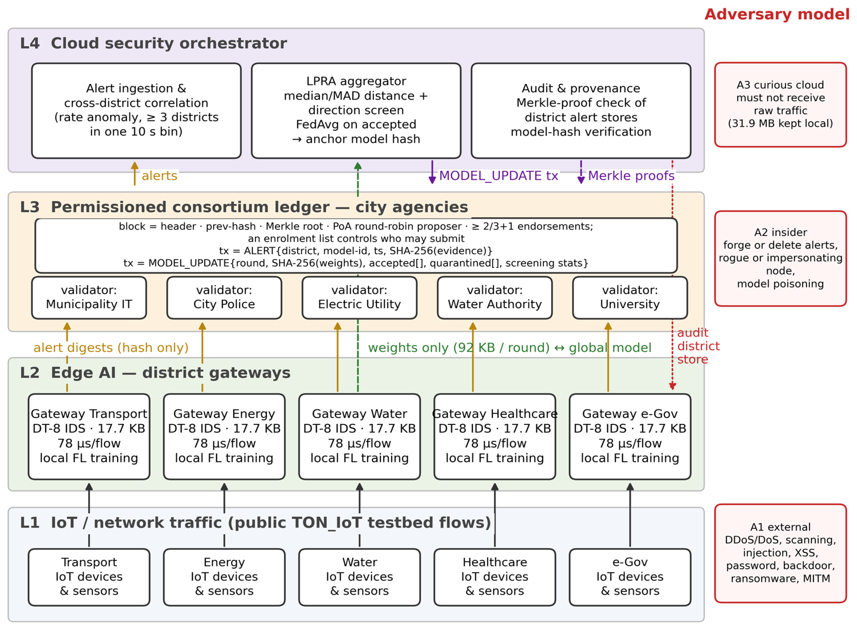
Figure 2.
(a) F1 with native versus common features; (b) edge footprint (latency vs. model size, log scale).
Figure 2.
(a) F1 with native versus common features; (b) edge footprint (latency vs. model size, log scale).
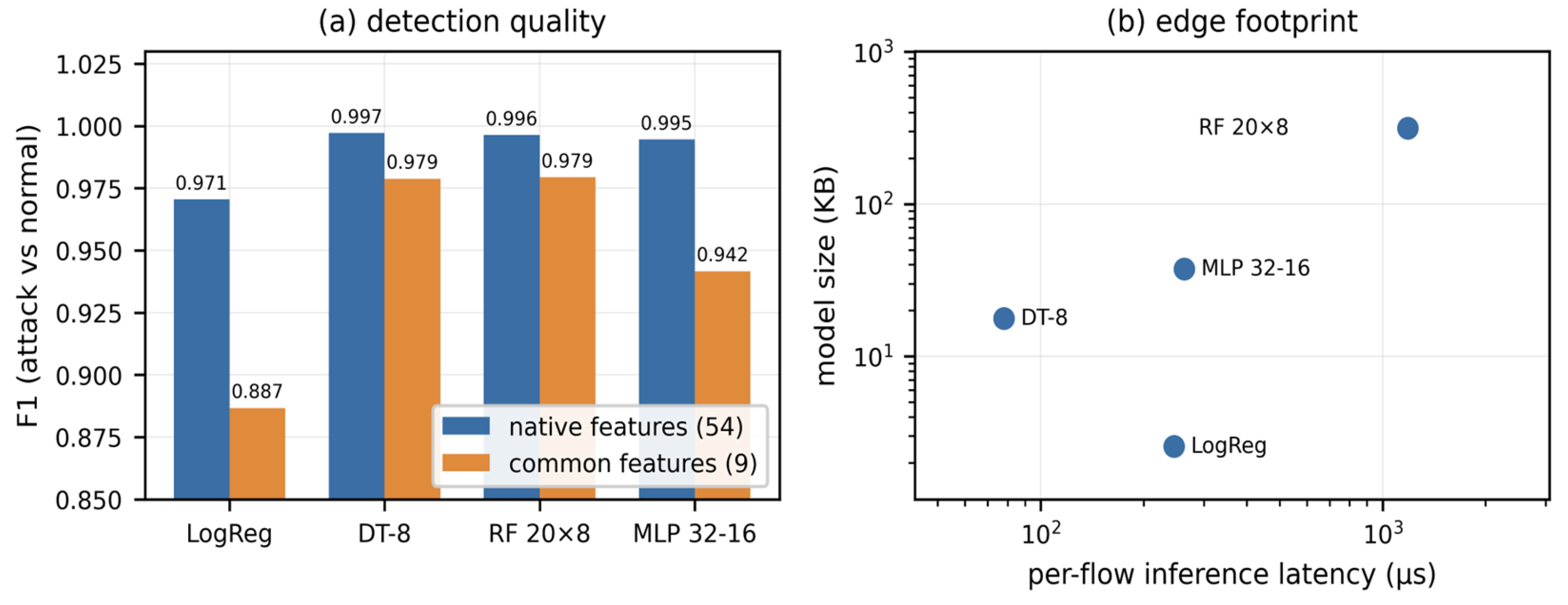
Figure 3.
Global-model F1 per communication round versus centralised and local-only baselines (seed 42).
Figure 3.
Global-model F1 per communication round versus centralised and local-only baselines (seed 42).
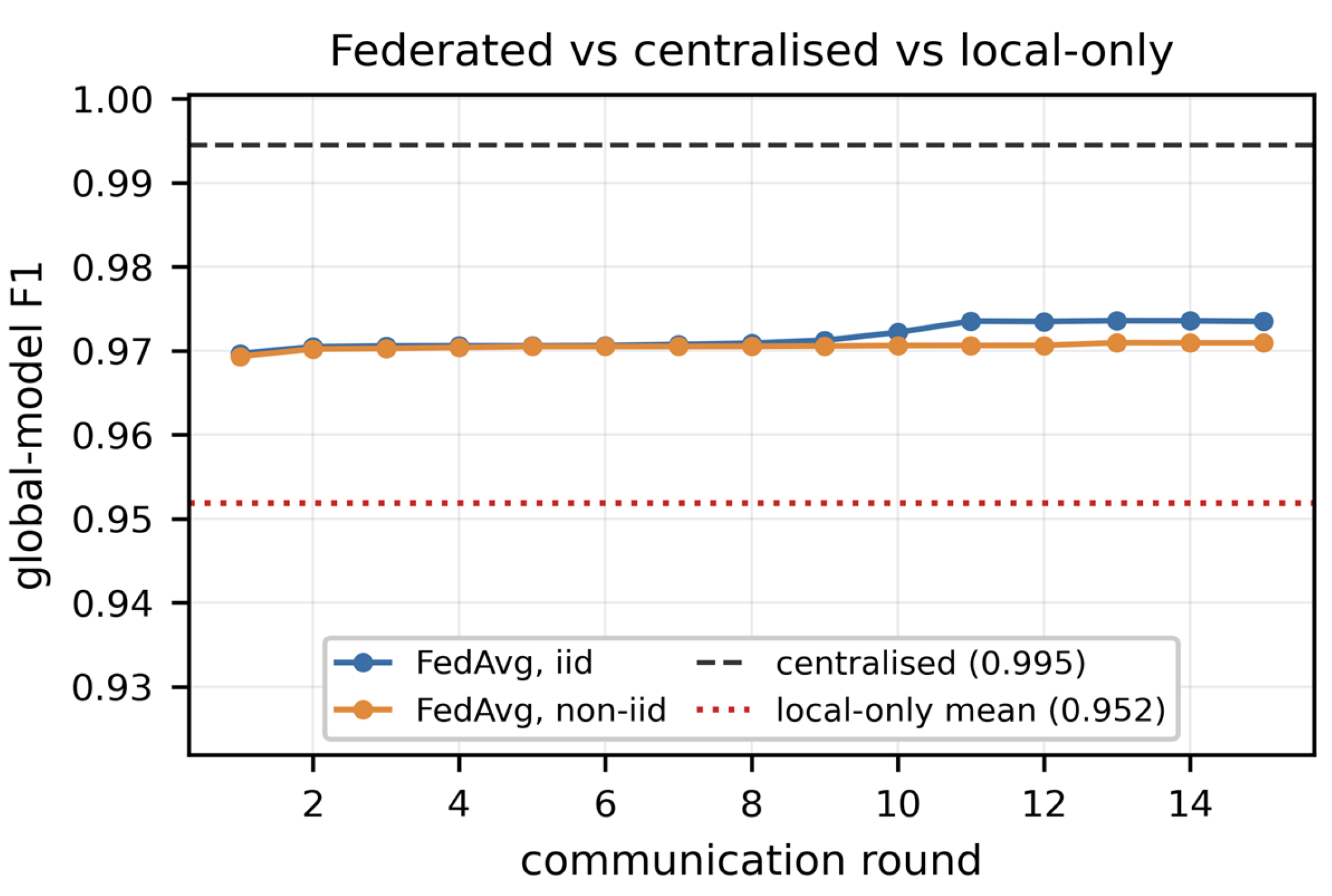
Figure 4.
Global F1 of six aggregators under four attacks with one (left) and two (right) Byzantine districts.
Figure 4.
Global F1 of six aggregators under four attacks with one (left) and two (right) Byzantine districts.
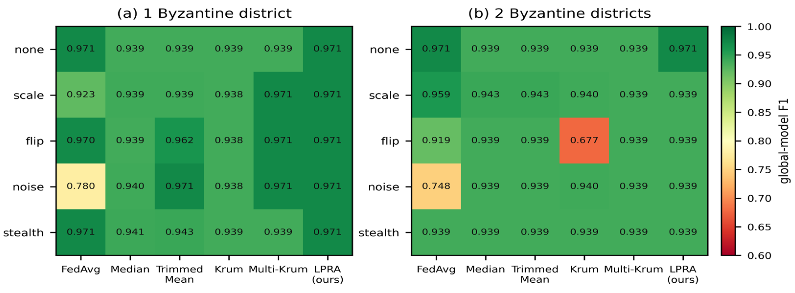
Figure 5.
Adaptive attacker sweep. The V-shaped red curve in (b) is the v1 failure: strong enough to dominate the stage-2 reference, not strong enough to fail the stage-1 distance test.
Figure 5.
Adaptive attacker sweep. The V-shaped red curve in (b) is the v1 failure: strong enough to dominate the stage-2 reference, not strong enough to fail the stage-1 distance test.
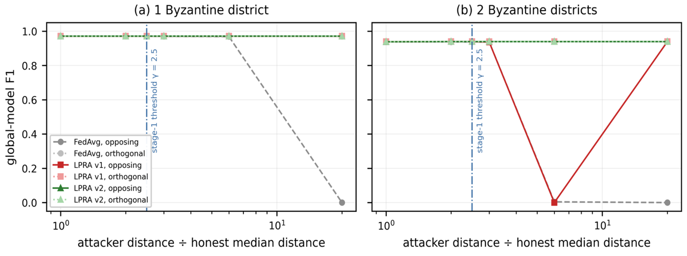
Figure 6.
Ledger storage overhead and latency (10,000 alert transactions, five validators).
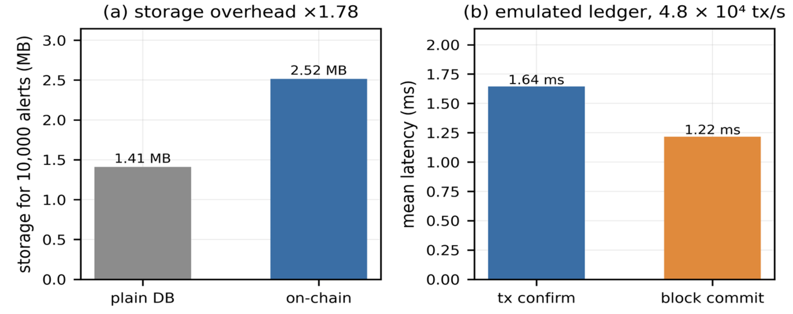
Figure 7.
Scalability: (a) districts with 20% Byzantine under “scale”; (b) ledger throughput and storage vs. validators; (c) block-size trade-off.
Figure 7.
Scalability: (a) districts with 20% Byzantine under “scale”; (b) ledger throughput and storage vs. validators; (c) block-size trade-off.
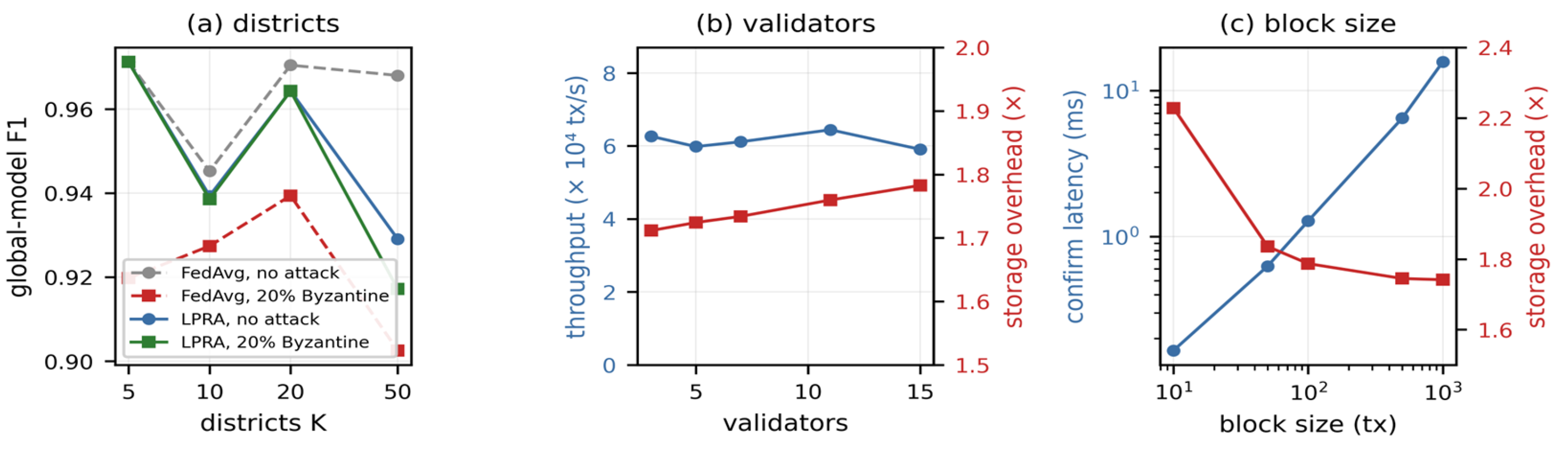
Figure 8.
Per-layer detection timeline in the replayed zero-day ransomware campaign: onset, first true edge alert, per-district rate anomaly, and the city-wide declaration.
Figure 8.
Per-layer detection timeline in the replayed zero-day ransomware campaign: onset, first true edge alert, per-district rate anomaly, and the city-wide declaration.
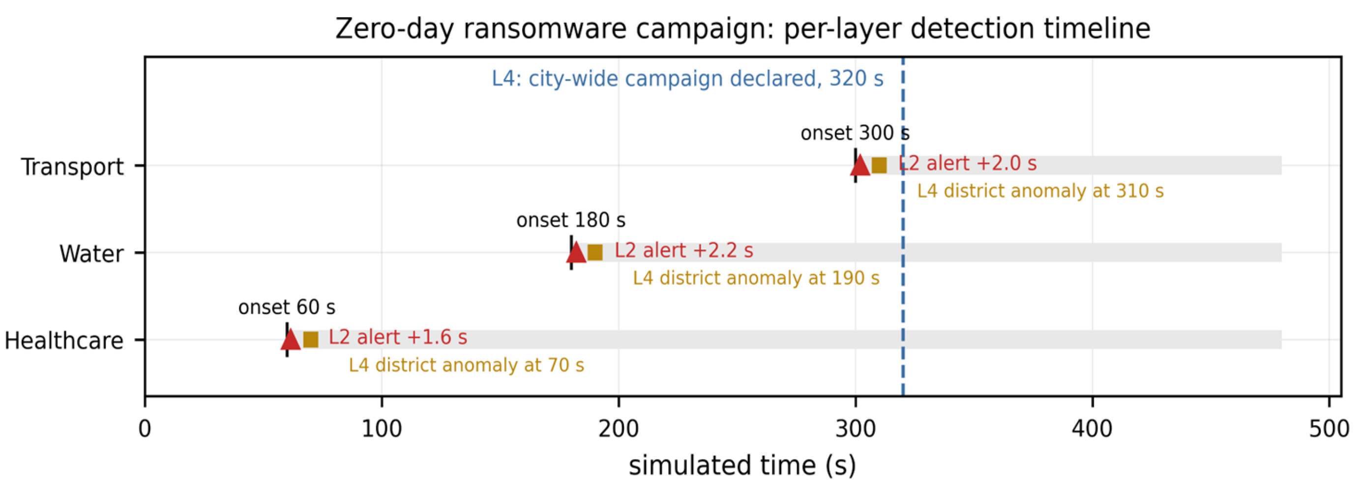
Figure 9.
Cross-dataset F1 (E12). (a) nine directional features; (b) four direction-free features. Rows are the training dataset, columns the held-out test split of the target dataset.
Figure 9.
Cross-dataset F1 (E12). (a) nine directional features; (b) four direction-free features. Rows are the training dataset, columns the held-out test split of the target dataset.
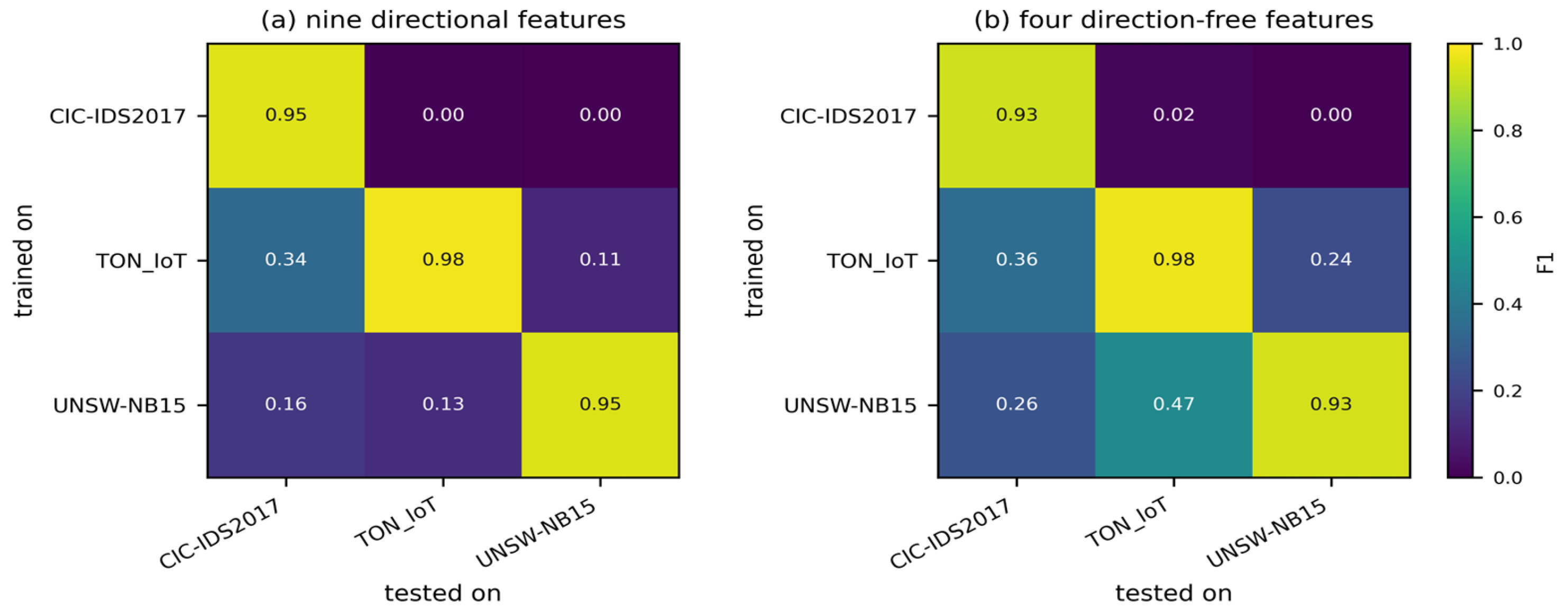
Figure 10.
(a) F1 per capture day for the static and rolling protocols against the random-split control; (b) recall on the two unseen days, static versus rolling.
Figure 10.
(a) F1 per capture day for the static and rolling protocols against the random-split control; (b) recall on the two unseen days, static versus rolling.
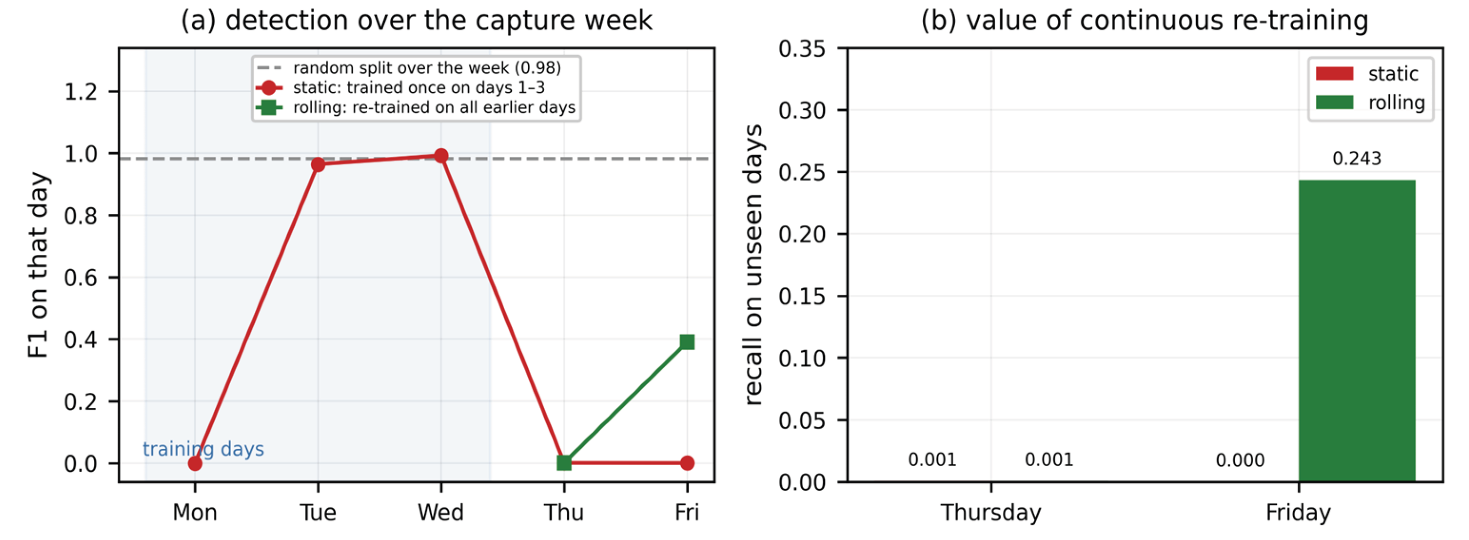

Table 1.
Threat model: adversaries, mitigating layer and the experiment that provides evidence.
| Adversary / attack | Layer & mechanism that mitigates | Evidence (experiment) |
| A1 volumetric & probing (DDoS, DoS, scanning) | L2 edge IDS | E1, E6 (unseen-family recall 0.94–1.00) |
| A1 application-level (injection, XSS, password, backdoor) | L2 edge IDS | E1, E6 (0.99–1.00) |
| A1 low-footprint (MITM, ransomware) | L2 edge IDS—partial | E6 (0.91 / 0.81, weakest cases) |
| A2-i forge or delete an alert after the fact | L3 Merkle root + L4 proof audit | E10 (1 forged alert detected, 0 false) |
| A2-ii inject alerts from a rogue or impersonating node | L3 membership (enrolment list) / endorsement | E10 (3 impostor identities rejected) |
| A2-iii poison the shared model (scale, flip, noise) | L4 LPRA screen + L3 anchored decision | E4, E5 (quarantined every round, F1 restored) |
| A2-iii adaptive stealth update | not mitigated (limitation) | E5 (undetected; no accuracy loss here) |
| A2-iii colluding majority of districts | outside model | — |
| A3 curious cloud reads raw traffic | L2 FL: weights only leave the district | E3 (31.9 MB raw kept local, 92 KB/round) |
Table 2.
Datasets and their role in the smart-city architecture. Row and feature counts are those produced by the released loader; per-dataset edge-IDS results are in Supplementary Table S3.
Table 2.
Datasets and their role in the smart-city architecture. Row and feature counts are those produced by the released loader; per-dataset edge-IDS results are in Supplementary Table S3.
| Dataset | Layer represented | Rows used | Classes | Native features (bias-aware) |
| TON_IoT (network) [12,13,14] | IoT district traffic | 211,043 | normal + 9 attacks | 54 |
| CIC-IDS2017 [16] | Enterprise / data centre | 300,000 | benign + 14 attacks | 89 |
| UNSW-NB15 [17] | Enterprise (2nd) | 200,000 | normal + 9 categories | 97 |
Table 3.
Experimental protocol. Multi-class attack typing and firewall-policy replication are reported in the Supplementary Material (Tables S1–S2).
Table 3.
Experimental protocol. Multi-class attack typing and firewall-policy replication are reported in the Supplementary Material (Tables S1–S2).
| ID (code) | Question | Setting |
| E1 (Exp-1/1b) | RQ1 edge model trade-off | LogReg, DT-8, RF 20×8, MLP (32,16); native (54) and common (9) features; F1, AUC, FPR, size, µs/flow, flows/s |
| E2 (Exp-12) | seed stability | E1 and E3 repeated with 5 seeds; mean ± SD |
| E3 (Exp-3) | RQ2 raw-data exposure and communication cost | FedAvg IID / non-IID vs centralised vs local-only; bytes kept local, weights per round; hashes anchored |
| E4 (Exp-9) | RQ2 poisoning | one Byzantine district: scale (λ = 10), label flip, Gaussian noise; plain FedAvg vs LPRA; no-attack control; personalised FL on each district’s own hold-out |
| E5 (Exp-11) | RQ2 baselines | LPRA vs FedAvg, Median, Trimmed Mean, Krum, Multi-Krum; 1–2 attackers; scale/flip/noise/stealth; 3 seeds; 60k-flow sample; 10 rounds |
| E6 (Exp-7) | validity | leave-one-attack-family-out: recall on the unseen family, FPR on held-out normal |
| E7 (Exp-8) | validity | random-forest importance ranking; DT-8 retrained after removing top-1/3/5/10/20 features |
| E8 (Exp-4) | RQ3 ledger cost | 10,000 alert tx, 5 validators, block 100; tx/s, confirm ms, storage vs plain DB; tamper test |
| E9 (Exp-13) | scalability | districts 5–50 with 20% Byzantine (LPRA vs FedAvg); validators 3–15; block size 10–1000; LPRA threshold sweep |
| E10 (Exp-5) | integration | 20,000 held-out flows through 5 gateways → ledger → cloud; latency, forged-alert audit, three impostor identities |
| E11 (Exp-14) | city scenario | zero-day ransomware campaign Healthcare→Water→Transport on a simulated clock (100 flows/s/district); time-to-detect per layer |
| E12 (Exp-1c/2) | cross-dataset | native benchmark per dataset; train on each, test on every other, on the common (9) and direction-free (4) views |
| E13 (fabric/) | RQ3 deployed permissioned ledger | same anchoring as chaincode on Hyperledger Fabric v2.5 test network (2 orgs, Raft); tx/s and latency at concurrency 20/50; ledger MB; non-member rejection |
| E14 (run_advanced.py --part T) | validity: temporal drift | CIC-IDS2017 evaluated chronologically by capture day: static (fit once on days 1–3) vs rolling (re-fit on every earlier day), with a random-split control; F1, recall, FPR and novelty per day |
| E15 (run_advanced.py --part R) | edge sustainability cost | per model: batch and single-flow CPU time, working set, serialised size, CPU-seconds and estimated energy per 106 flows on a stated board power |
| E16 (run_advanced.py --part A) | RQ2 adaptive adversary | attacker that knows the screen, placed at s × the honest median distance, opposing or orthogonal; s swept over two orders of magnitude; FedAvg vs LPRA v1 vs LPRA v2 |
Table 4.
Edge IDS benchmark on TON_IoT (54 bias-aware native features, 70/30 stratified split, single CPU core, seed 42). Five-seed means and SDs are given in Section 5.4.
Table 4.
Edge IDS benchmark on TON_IoT (54 bias-aware native features, 70/30 stratified split, single CPU core, seed 42). Five-seed means and SDs are given in Section 5.4.
| Model | Acc. | F1 | ROC-AUC | FPR | Serialised size (KB) | Latency (µs/flow) | Throughput (flows/s) |
| Logistic regression | 0.954 | 0.971 | 0.982 | 0.163 | 2.6 | 246 | 5.7 × 10⁶ |
| Decision tree (d = 8) | 0.996 | 0.997 | 0.997 | 0.009 | 17.7 | 78 | 1.2 × 10⁷ |
| Random forest (20 × 8) | 0.994 | 0.996 | 0.999 | 0.016 | 314.3 | 1184 | 6.4 × 10⁵ |
| MLP (32, 16) | 0.992 | 0.995 | 0.998 | 0.025 | 37.4 | 263 | 3.1 × 10⁶ |
Table 5.
Same models on the nine common semantic features (TON_IoT).
| Model | Acc. | F1 | ROC-AUC | FPR |
| Logistic regression | 0.806 | 0.887 | 0.822 | 0.800 |
| Decision tree (d = 8) | 0.967 | 0.979 | 0.977 | 0.130 |
| Random forest (20 × 8) | 0.968 | 0.979 | 0.982 | 0.132 |
| MLP (32, 16) | 0.910 | 0.942 | 0.924 | 0.244 |
Table 6.
Federated versus centralised versus local-only training (five districts, TON_IoT).
| Regime | Local-only mean F1 | FedAvg F1 | Centralised F1 | Raw data kept private | Weights / round |
| IID (seed 42) | 0.972 | 0.973 | 0.995 | 31.9 MB | 92 KB |
| Non-IID (5 seeds, mean ± SD) | 0.952 ± 0.002 | 0.971 ± 0.001 | 0.994 | 31.9 MB | 92 KB |
Table 7.
Global-model F1 with one of five districts Byzantine (non-IID TON_IoT, full data). The control row reports false quarantines instead of rounds quarantined.
Table 7.
Global-model F1 with one of five districts Byzantine (non-IID TON_IoT, full data). The control row reports false quarantines instead of rounds quarantined.
| Attack by Byzantine district | Plain FedAvg F1 | LPRA F1 | Rounds quarantined (LPRA) |
| none (control) | 0.971 | 0.971 | 0 false quarantines / 75 |
| scaled update (λ = 10) | 0.866 | 0.971 | 15 / 15 |
| label flipping | 0.972 | 0.971 | 15 / 15 |
| Gaussian-noise weights | 0.686 | 0.971 | 15 / 15 |
Table 8.
Personalised FL: one local epoch after convergence, evaluated on each district’s own hold-out.
Table 8.
Personalised FL: one local epoch after convergence, evaluated on each district’s own hold-out.
| District | Global model F1 (own test) | Personalised F1 (own test) | Gain (F1 pts) |
| Transport | 0.977 | 0.983 | +0.6 |
| Energy | 0.973 | 0.975 | +0.2 |
| Water | 0.969 | 0.982 | +1.3 |
| Healthcare | 0.978 | 0.981 | +0.3 |
| e-Government | 0.919 | 0.932 | +1.3 |
Table 9.
Global-model F1 (mean over 3 seeds; ± SD shown when ≥ 0.005) with 0–2 of 5 districts Byzantine, 60k-flow sample, 10 rounds. ✓ = attacker(s) quarantined in ≥ 8 of 10 rounds; a fraction gives the quarantine rate when it is lower; † = at least one honest district rejected per round on average. Per-rule quarantine rates, honest-rejection counts and no-attack F1 are tabulated separately in Supplementary Table S7, since the marks compress three quantities into one symbol.
Table 9.
Global-model F1 (mean over 3 seeds; ± SD shown when ≥ 0.005) with 0–2 of 5 districts Byzantine, 60k-flow sample, 10 rounds. ✓ = attacker(s) quarantined in ≥ 8 of 10 rounds; a fraction gives the quarantine rate when it is lower; † = at least one honest district rejected per round on average. Per-rule quarantine rates, honest-rejection counts and no-attack F1 are tabulated separately in Supplementary Table S7, since the marks compress three quantities into one symbol.
| Attack (attackers) | FedAvg | Median | Trimmed Mean | Krum | Multi-Krum | LPRA (ours) |
| none (0) | 0.971 | 0.939 | 0.939 | 0.939 † | 0.939 † | 0.971 |
| scale (1) | 0.923 ± 0.014 | 0.939 | 0.939 | 0.938 ✓ † | 0.971 ✓ | 0.971 ✓ |
| flip (1) | 0.970 | 0.939 | 0.962 | 0.938 ✓ † | 0.971 ✓ | 0.971 ✓ |
| noise (1) | 0.780 ± 0.161 | 0.940 ± 0.011 | 0.971 | 0.938 ✓ † | 0.971 ✓ | 0.971 ✓ |
| stealth (1) | 0.971 | 0.941 | 0.943 | 0.939 ✓ † | 0.939 † | 0.971 |
| scale (2) | 0.959 ± 0.020 | 0.943 ± 0.005 | 0.943 ± 0.005 | 0.940 ✓ † | 0.939 ✓ | 0.939 ✓ |
| flip (2) | 0.919 ± 0.013 | 0.939 | 0.939 | 0.677 ± 0.456 (7/10) † | 0.939 ✓ | 0.939 ✓ |
| noise (2) | 0.748 ± 0.080 | 0.939 | 0.939 | 0.940 ✓ † | 0.939 ✓ | 0.939 ✓ |
| stealth (2) | 0.939 | 0.939 | 0.939 | 0.939 † | 0.939 † | 0.939 |
Table 10.
Adaptive attacker that knows the screen (E16): global-model F1 after 10 rounds, with the number of rounds in which every attacker was quarantined in parentheses. s is the attacker’s distance from the honest median as a multiple of the honest median distance; the stage-1 threshold sits at γ = 2.5.
Table 10.
Adaptive attacker that knows the screen (E16): global-model F1 after 10 rounds, with the number of rounds in which every attacker was quarantined in parentheses. s is the attacker’s distance from the honest median as a multiple of the honest median distance; the stage-1 threshold sits at γ = 2.5.
| Attackers | Direction | Strength s | FedAvg | LPRA v1 | LPRA v2 |
| 1 | orthogonal | 1 | 0.971 | 0.971 (0/10) | 0.971 (0/10) |
| 1 | orthogonal | 2 | 0.971 | 0.971 (0/10) | 0.971 (0/10) |
| 1 | orthogonal | 2.5 | 0.971 | 0.971 (0/10) | 0.971 (0/10) |
| 1 | orthogonal | 3 | 0.971 | 0.971 (3/10) | 0.971 (3/10) |
| 1 | orthogonal | 6 | 0.971 | 0.971 (10/10) | 0.971 (10/10) |
| 1 | orthogonal | 20 | 0.970 | 0.971 (10/10) | 0.971 (10/10) |
| 1 | opposite | 1 | 0.971 | 0.971 (6/10) | 0.971 (5/10) |
| 1 | opposite | 2 | 0.971 | 0.971 (10/10) | 0.971 (10/10) |
| 1 | opposite | 2.5 | 0.971 | 0.971 (10/10) | 0.971 (10/10) |
| 1 | opposite | 3 | 0.970 | 0.971 (10/10) | 0.971 (10/10) |
| 1 | opposite | 6 | 0.969 | 0.971 (10/10) | 0.971 (10/10) |
| 1 | opposite | 20 | 0.000 | 0.971 (10/10) | 0.971 (10/10) |
| 2 | orthogonal | 1 | 0.939 | 0.939 (0/10) | 0.939 (0/10) |
| 2 | orthogonal | 2 | 0.939 | 0.939 (0/10) | 0.939 (0/10) |
| 2 | orthogonal | 2.5 | 0.939 | 0.939 (0/10) | 0.939 (0/10) |
| 2 | orthogonal | 3 | 0.939 | 0.939 (4/10) | 0.939 (4/10) |
| 2 | orthogonal | 6 | 0.939 | 0.939 (10/10) | 0.939 (10/10) |
| 2 | orthogonal | 20 | 0.938 | 0.939 (10/10) | 0.939 (10/10) |
| 2 | opposite | 1 | 0.938 | 0.938 (0/10) | 0.938 (0/10) |
| 2 | opposite | 2 | 0.938 | 0.939 (10/10) | 0.939 (10/10) |
| 2 | opposite | 2.5 | 0.937 | 0.939 (10/10) | 0.939 (10/10) |
| 2 | opposite | 3 | 0.937 | 0.937 (6/10) | 0.939 (10/10) |
| 2 | opposite | 6 | 0.004 | 0.000 (0/10) | 0.939 (10/10) |
| 2 | opposite | 20 | 0.000 | 0.939 (10/10) | 0.939 (10/10) |
Table 11.
Leave-one-attack-family-out (depth-8 tree, 54 native features, TON_IoT).
| Held-out family | Unseen samples | Recall on unseen | FPR (normal) |
| backdoor | 20,000 | 1.000 | 0.009 |
| ddos | 20,000 | 0.988 | 0.018 |
| dos | 20,000 | 0.945 | 0.009 |
| injection | 20,000 | 0.998 | 0.009 |
| mitm | 1,043 | 0.913 | 0.009 |
| password | 20,000 | 0.998 | 0.011 |
| ransomware | 20,000 | 0.808 | 0.010 |
| scanning | 20,000 | 1.000 | 0.014 |
| xss | 20,000 | 0.989 | 0.010 |
Table 12.
Feature-importance ablation (depth-8 tree after removing the k most important features).
| Top-k features removed | Features left | F1 | Removed features |
| 0 | 54 | 0.997 | — |
| 1 | 53 | 0.996 | pkt_ratio |
| 3 | 51 | 0.997 | + src_pkts, proto_udp |
| 5 | 49 | 0.970 | + src_ip_bytes, proto_tcp |
| 10 | 44 | 0.943 | + dns_qtype, dst_ip_bytes, dst_pkts, duration, byte_ratio |
| 20 | 34 | 0.939 | + service_dns, conn_state_S0, has_dns, bytes_per_pkt_dst, dns_rejected, dns_qclass… |
Table 13.
Scaling the number of districts with 20% Byzantine under the scaling attack (10 rounds, seed 42, 60k-flow sample).
Table 13.
Scaling the number of districts with 20% Byzantine under the scaling attack (10 rounds, seed 42, 60k-flow sample).
| Districts K | Byzantine | FedAvg F1 (no attack) | LPRA F1 (no attack) | FedAvg F1 (scale) | LPRA F1 (scale) | Attackers quarantined | Honest rejections |
| 5 | 1 | 0.971 | 0.971 | 0.920 | 0.971 | 10 / 10 | 0 / 50 |
| 10 | 2 | 0.945 | 0.939 | 0.927 | 0.939 | 10 / 10 | 4 / 100 |
| 20 | 4 | 0.970 | 0.964 | 0.939 | 0.964 | 10 / 10 | 80 / 200 |
| 50 | 10 | 0.968 | 0.929 | 0.903 | 0.917 | 10 / 10 | 90 / 500 |
Table 14.
(a). Cross-dataset F1 on the nine directional common features (E12). Rows are the training dataset, columns the held-out test split of the target dataset. (b). The same experiment on the four direction-free features, the view that also admits datasets without a directional split.
Table 14.
(a). Cross-dataset F1 on the nine directional common features (E12). Rows are the training dataset, columns the held-out test split of the target dataset. (b). The same experiment on the four direction-free features, the view that also admits datasets without a directional split.
| Train \ Test | CIC-IDS2017 | TON_IoT | UNSW-NB15 |
| (a) | |||
| CIC-IDS2017 | 0.95 | 0.00 | 0.00 |
| TON_IoT | 0.34 | 0.98 | 0.11 |
| UNSW-NB15 | 0.16 | 0.13 | 0.95 |
| (b) | |||
| CIC-IDS2017 | 0.93 | 0.02 | 0.00 |
| TON_IoT | 0.36 | 0.98 | 0.24 |
| UNSW-NB15 | 0.26 | 0.47 | 0.93 |
Table 15.
Emulated ledger (Section 5.5) versus an equivalent anchoring interface on a Hyperledger Fabric v2.5.9 test network with two organisations and Raft ordering (E13). The Fabric rows are the mean of 2,000 anchored alerts per run; block cutting at 10 messages or 2 s; storage in decimal MB per 10,000 alerts throughout.
Table 15.
Emulated ledger (Section 5.5) versus an equivalent anchoring interface on a Hyperledger Fabric v2.5.9 test network with two organisations and Raft ordering (E13). The Fabric rows are the mean of 2,000 anchored alerts per run; block cutting at 10 messages or 2 s; storage in decimal MB per 10,000 alerts throughout.
| Setting | tx/s | Latency mean (ms) | p50 (ms) | p95 (ms) | p99 (ms) | Ledger MB per 10,000 alerts |
| Emulated ledger, 5 validators (Section 5.5) | 47,744 | 1.6 | — | — | — | 2.5 |
| Fabric v2.5.9, 2 orgs, Raft, concurrency 20 | 146 | 136 | 126 | 216 | 338 | 60.8 |
| Fabric v2.5.9, 2 orgs, Raft, concurrency 50 | 134 | 278 | 263 | 375 | 466 | 60.8 |
Table 16.
Chronological evaluation on CIC-IDS2017 (E14). The static model is fitted once on the pooled traffic of Monday–Wednesday, not one model per day. Rows marked in-sample are evaluations on data that model was fitted on and are reported only to show that the fit succeeded; they are not held-out scores. Rolling re-fits on every earlier day before each test day, so its rows are held out. F1 and recall are undefined on a day with no attack flows—Monday’s attack share is zero—and are shown as —.
Table 16.
Chronological evaluation on CIC-IDS2017 (E14). The static model is fitted once on the pooled traffic of Monday–Wednesday, not one model per day. Rows marked in-sample are evaluations on data that model was fitted on and are reported only to show that the fit succeeded; they are not held-out scores. Rolling re-fits on every earlier day before each test day, so its rows are held out. F1 and recall are undefined on a day with no attack flows—Monday’s attack share is zero—and are shown as —.
| Protocol | Day | Evaluation | Flows | Attack share | F1 | Recall | FPR |
| static | monday | in-sample | 120,000 | 0.0000 | — | — | 0.0020 |
| static | tuesday | in-sample | 120,000 | 0.0312 | 0.9643 | 0.9786 | 0.0016 |
| static | wednesday | in-sample | 120,000 | 0.3639 | 0.9928 | 0.9892 | 0.0020 |
| static | thursday | held out | 240,000 | 0.0065 | 0.0010 | 0.0006 | 0.0022 |
| static | friday | held out | 360,000 | 0.3773 | 0.0005 | 0.0003 | 0.0095 |
| rolling | thursday | held out | 240,000 | 0.0065 | 0.0010 | 0.0006 | 0.0022 |
| rolling | friday | held out | 360,000 | 0.3773 | 0.3908 | 0.2434 | 0.0014 |
Table 17.
Novelty per capture day: what the model had never seen when it met that day.
| Day | Attack families appearing for the first time |
| monday | (none new) |
| tuesday | ftp—patator, ssh—patator |
| wednesday | dos goldeneye, dos hulk, dos slowhttptest, dos slowloris, heartbleed |
| thursday | infiltration, web attack—brute force, web attack—sql injection, web attack—xss |
| friday | bot, ddos, portscan |
Table 18.
Edge cost per model (E15), profiled on the same models and the same training split as Table 4, so the serialised sizes are identical in both tables. Assumptions for the two right-hand columns: 3 W assumed board power, 1,000 flows/s sustained rate, energy obtained by scaling measured CPU time rather than by a wattmeter, and detection only—the network interface, storage, TLS, ledger anchoring and cooling are excluded. The CPU-seconds column allows rescaling to other assumptions.
Table 18.
Edge cost per model (E15), profiled on the same models and the same training split as Table 4, so the serialised sizes are identical in both tables. Assumptions for the two right-hand columns: 3 W assumed board power, 1,000 flows/s sustained rate, energy obtained by scaling measured CPU time rather than by a wattmeter, and detection only—the network interface, storage, TLS, ledger anchoring and cooling are excluded. The CPU-seconds column allows rescaling to other assumptions.
| Model | Batch CPU (µs/flow) | Single flow (µs) | Runtime working set (MB) | Serialised size (KB) | CPU-s / 106 flows | J / 106 flows (3 W) | kWh/year (3 W) |
| Logistic regression | 0.190 | 222 | 1.85 | 2.6 | 0.190 | 0.57 | 0.005 |
| Decision tree (d = 8) | 0.064 | 74 | 0.25 | 17.7 | 0.064 | 0.19 | 0.002 |
| Random forest (20 × 8) | 0.909 | 1094 | 0.34 | 314.3 | 0.909 | 2.73 | 0.024 |
| MLP (32, 16) | 0.356 | 233 | 3.19 | 37.4 | 0.356 | 1.07 | 0.009 |
Disclaimer/Publisher’s Note: The statements, opinions and data contained in all publications are solely those of the individual author(s) and contributor(s) and not of MDPI and/or the editor(s). MDPI and/or the editor(s) disclaim responsibility for any injury to people or property resulting from any ideas, methods, instructions or products referred to in the content. |
© 2026 by the authors. Licensee MDPI, Basel, Switzerland. This article is an open access article distributed under the terms and conditions of the Creative Commons Attribution (CC BY) license (http://creativecommons.org/licenses/by/4.0/).
Copyright: This open access article is published under a Creative Commons CC BY 4.0 license, which permit the free download, distribution, and reuse, provided that the author and preprint are cited in any reuse.