
Submitted:
23 August 2026
Posted:
24 August 2026
You are already at the latest version
Abstract
This research develops a 12-week rolling-horizon mixed-integer programming model with an ECO-centric objective to address scheduling inconsistency caused by frequent engineering change orders (ECOs), incomplete bills of materials (BOMs), and production-line imbalance in server assembly. The model integrates BOM versions, workstation capacities, worker shifts, order priorities, and SLA constraints, while incorporating event-triggered incremental rescheduling, historical-solution warm starts, variable freezing, and adaptive neighborhood expansion. Eighteen months of production data from a server manufacturer in California, USA, were used for discrete-event simulation and validation. Results show that the proposed method reduces cumulative delay to 2,026 hours, overdue work orders to 121, peak work-in-process to 286 units, and schedule recovery time to 21.7 hours. The approach maintains schedule stability and production-capacity balance under multiple concurrent disturbances, providing a computationally feasible decision-support solution for dynamic scheduling in high-mix, low-volume server assembly environments, improving responsiveness to engineering changes, material shortages, equipment downtime, and rush orders.
Keywords:
server assembly
; engineering changes
; rolling scheduling
; mixed-integer programming
; capacity balancing
1. Introduction
Server assembly involves product variants, low-volume production, deep BOM hierarchies, and frequent ECO changes, which can cause material mismatches, workstation congestion, and schedule fluctuations. Lu et al. developed a multi-product mixed-integer programming model considering degradation effects to improve scheduling computability [1]; Hao et al. applied adaptive multi-class support vector machines for system reliability evaluation and dynamic state identification [2]; Yi et al. examined dynamic scheduling in flexible workshops under multiple event types [3]; Liu et al. incorporated start-stop strategies and time-of-use electricity pricing into green scheduling [4]. Lanzani et al. and Ali et al. explored virtual-physical mapping for digital-twin integration in discrete manufacturing systems and the evolution of simulation models, respectively [5,6]. However, approaches address single disturbances or fixed resource allocation, with limited consideration of ECO propagation combined with material shortages, downtime, and inserted orders. To address these limitations, a 12-week rolling mixed-integer programming model integrates BOM versions, workcell capacities, shifts, SLAs, and capacity imbalance, supported by event-triggered rescheduling, warm starts, variable freezing, and adaptive neighborhood expansion. Simulation results show reduced delay, WIP peaks, and recovery time under complex disturbances.
2. Modeling of Disturbance Scheduling for Server Assembly
Server assembly scheduling integrates production work orders, bills of material (BOM), engineering change orders (ECO), workstation operation records, and material shortage records to construct associations among work orders, materials, processes, workstations, and equipment states. Cross-system data are mapped using work-order numbers, product configuration codes, and BOM versions, while records with missing labour hours, abnormal downtime, or duplicates are removed [7]. When ECOs modify materials, processes, or labor hours, an impact-propagation chain identifies affected work orders and downstream processes. Ad hoc orders, material delays, and line downtime are captured as disturbances to update capacities, staffing, priorities, and rescheduling states in time.
3. Capacity-Balancing-Driven Rolling Scheduling Model
3.1. Twelve-Week Rolling Time-Domain Framework
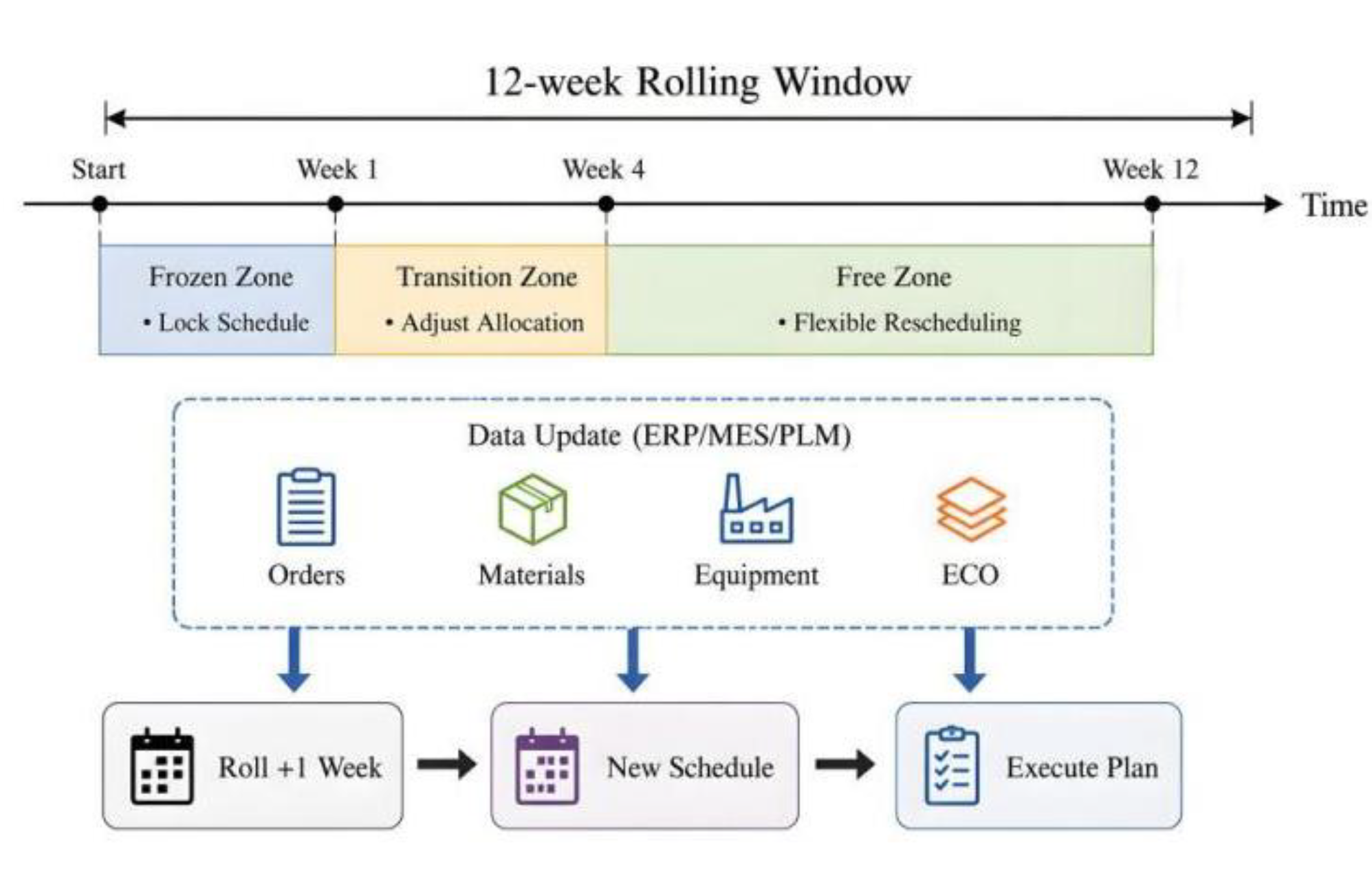
Figure 1.
Twelve-Week Rolling Window and Freeze Strategy Diagram.
3.2. Multi-Objective Function Design
The scheduling objective simultaneously addresses delivery lead times, production changeovers, overtime resources, work-in-process (WIP) occupancy, and SLA violations:
The production capacity imbalance is defined as:
3.3. Assembly Constraint Construction
Workstation capacity constraints are generated based on normal shifts, equipment availability, and permitted overtime:
Material and process feasibility are subject to joint constraints:
3.4. Event-Triggered Dynamic Rescheduling Algorithm
As shown in Figure 2, the MES Event Bus continuously receives ECOs, material shortages, equipment downtime, and ad-hoc orders. The Event Analysis Module converts each message into event type, occurrence time, affected work order, resource loss, and estimated duration. Incremental rescheduling is triggered when estimated delay exceeds 4 h, downtime exceeds 2 h, ad-hoc orders reach 50 units, or a critical BOM version changes. The affected neighborhood is defined as:
4. Discrete-Event Simulation and Experimental Validation
4.1. Simulation Environment and Parameters
The experimental platform consists of an Intel Xeon Gold 6430 processor, 128 GB memory and the operating system Ubuntu 22.04. The scheduling program is coded in Python 3.11, the mixed-integer programming model is solved with Gurobi 11.0 and the discrete-event simulation is developed with SimPy 4.1. The 18-month data set was split into three periods: the initial 12 months for parameter calibration, the next 3 months for weight adjustment and the last 3 months for free testing. Servers, workstations and racks had established assembly, burning of the firmware, functional testing and aging testing processes. The number of labor hours distributed were based on 31, 752 workstation records by product family and process. The upper limit for daily rescheduling was fixed to 180 seconds and relative optimal buffer to 1% and the upper limit for the weekly model to 600 seconds. Each scenario used 60 runs with distinct seeds 2026-2085; all methods used the same seed in each run for common random numbers, and each metric was summarized by its mean, standard deviation, and 95% confidence interval across runs.
4.2. Multi-Disturbance Scenario Setup
The perturbation injector sends material delays, production-line downtime, ad-hoc orders, and ECO events by timestamp to the simulation event queue. Delivery delays were set to 3, 5, 7, and 10 days; line shutdowns to 8, 16, 24, and 40 hours; ad-hoc orders to 50, 100, 150, and 200 units; and ECO frequencies to 10, 20, and 30 per week. Single-disturbance scenarios were used to identify response boundaries, while composite scenarios included material shortages with order insertions, downtime with ECOs, and all four disturbance types. The coefficient of variation for processing time was randomly sampled from 0.08 to 0.20, and 4.6%–18.2% of work orders were affected by ECOs distributed across the frozen and transition zones. To ensure fair scheduling comparisons, all methods used identical disturbance-event sequences and the same initial production-capacity snapshot, thereby preventing sample differences from influencing performance evaluation under both isolated and coupled disturbance conditions in every experimental replication.
4.3. Comparison of Scheduling Performance
Four methods were compared: manual priority dispatching without optimization, static MIP solved once, fixed-cycle rolling MIP solved weekly, and event-triggered rolling MIP. The three MIP-based methods used the same objective, constraints, Gurobi 11.0, 1% gap, hardware, and equivalent solution-time limits at the corresponding scheduling level.. Testing used 394 work orders, 71 BOM versions, 47 ECOs, and four disturbance types from records.
Incremental rolling scheduling reduced mean overdue work orders by 28, cumulative delay by 18.2%, and recovery time by 7.2 h compared with fixed-cycle rolling. Across 60 replications, the 95% confidence intervals for these principal metrics remained narrow and non-overlapping. Weekly average completions, defined as server units completing all required assembly and testing operations per week, increased by 2.5%, while peak WIP decreased by 25 units. Figure 3 further shows nonlinear performance degradation as coupled disturbances intensify.

Table 1.
Comparison of Overall Performance Among Different Scheduling Methods.
| Scheduling Method | Overdue Orders / count | Cumulative Delay / h | Weekly Completions / units·week⁻¹ | Peak WIP / units | Idle Time / h | Rescheduling Events / count | Recovery Time / h |
| Manual Priority Scheduling | 238 ± 12 (234.9–241.1) | 3826 ± 165 (3783.4–3868.6) | 184 ± 8 (181.9–186.1) | 368 ± 15 (364.1–371.9) | 436 ± 20 (430.8–441.2) | 96 ± 7 (94.2–97.8) | 46.8 ± 2.6 (46.1–47.5) |
| Static Mixed-Integer Programming | 191 ± 10 (188.4–193.6) | 3104 ± 142 (3067.3–3140.7) | 191 ± 7 (189.2–192.8) | 342 ± 14 (338.4–345.6) | 371 ± 18 (366.4–375.6) | 84 ± 6 (82.5–85.5) | 38.6 ± 2.2 (38.0–39.2) |
| Fixed-Cycle Rolling Schedule | 149 ± 8 (146.9–151.1) | 2478 ± 116 (2448.0–2508.0) | 199 ± 6 (197.5–200.5) | 311 ± 12 (307.9–314.1) | 318 ± 15 (314.1–321.9) | 73 ± 5 (71.7–74.3) | 28.9 ± 1.8 (28.4–29.4) |
| Event-Triggered Incremental Rolling Scheduling | 121 ± 7 (119.2–122.8) | 2026 ± 94 (2001.7–2050.3) | 204 ± 5 (202.7–205.3) | 286 ± 10 (283.4–288.6) | 275 ± 13 (271.6–278.4) | 61 ± 4 (60.0–62.0) | 21.7 ± 1.4 (21.3–22.1) |
In Figure 3(a), increasing ECO frequency and downtime raise cumulative delay from about 1,550 h to over 2,680 h. Figure 3(b) shows recovery time increasing from 13 to 34 h as material delay rises from 3 to 10 days and inserted orders from 50 to 200 units. Figure 3(c) indicates sustained high loads at functional and aging-testing workstations before rescheduling. Event-triggered incremental rescheduling redistributes overloaded tasks across neighboring cycles and alternative workstations. Figure 3(d) reports utilization variance of 0.091 with cumulative delay of 2,026 h, while maintaining lower peak WIP and stable schedules. These results confirm gains from localized capacity migration rather than expansion.
4.4. Stability and Ablation Analysis
The ECO influence propagation, the hot start, the variable freezing, the adaptive neighborhood, and the capacity balance conditions were removed in sequence under the conditions of 0.16, 20 ECOs/week, and 24 hours off; the results are shown in Table 2.
Across 60 replications, removing the warm start increased average solution time from 48.6±4.1 s to 96.7±8.6 s, with non-overlapping 95% confidence intervals, confirming the computational value of historical feasible solutions. Removing variable freezing reduced cumulative delay from 2026±94 h to 1987±92 h, but rescheduling events increased from 61±4 to 104±7 and recovery time rose from 21.7±1.4 h to 28.2±2.0 h, revealing a tradeoff between delay reduction and schedule stability. Removing the capacity-balancing term increased utilization dispersion from 0.091±0.006 to 0.156±0.011.
Figure 4(b) shows that the adaptive neighborhood first releases directly affected work orders, then progressively includes transition-zone orders, shared-resource orders, and adjacent orders as disturbance propagation expands. Figure 4(c) shows that the full model reaches the target optimality gap at about 48.6 s, whereas models without warm start or adaptive neighborhood converge more slowly. Figure 4(d) shows recovery times of 21.7 h for the full model, 26.9 h without ECO propagation, 25.7 h without adaptive neighborhood, and 28.2 h without variable freezing. These results indicate that each module supports a distinct performance dimension and that gradual neighborhood expansion improves recovery while preserving schedule stability under coupled disturbances and avoiding unnecessary full-space schedule changes during repeated dynamic optimization cycles in practice.
5. Conclusions
A 12-week rolling time domain model was developed, and incremental rescheduling was realized through event triggering, historical solution-based restart, variable freezing, and adaptive neighborhood expansion to deal with the frequent disturbances due to engineering change, material delay, equipment downtime, and ad hoc orders. Experiments indicate that this approach leads to fewer overdue work orders, fewer cumulative delays, a lower maximum work-in-progress and a shorter schedule recovery time, and also increases the distribution of work orders among the workstations. The current model still uses historical labour hour distributions and assumes the levels of disturbances, and it is unable to adequately consider changes in supplier lead time, variations in worker skill or multi-plant co-operation. Future research ideas are to implement online learning to update processing time parameters, to use digital twins to synchronize the scheduling states across production lines, and to explore a combined solution mechanism to leverage cross-production-line reinforcement learning and MIP to improve real-time decision-making capabilities under complicated disturbances.
References
- Lu, S.; Chen, Y.; Zheng, R.; et al. A mixed-integer programming model and dynamic programming-based approach for multi-product production scheduling under deterioration effects [J]. Comput. Oper. Res. 2026, 194107596–107596. [Google Scholar] [CrossRef]
- Hao, Z.; Zhang, D.; Dai, S.; et al. A novel adaptive multi-class probability support vector machine model for evidence theory-based system reliability analysis[J]. Reliab. Eng. Syst. Saf. 2027, 277(P3), 113116–113116. [Google Scholar] [CrossRef]
- Yi, W.; Deng, Q.; Wang, B.; et al. Dynamic flexible job shop scheduling problem considering multiple types of dynamic events [J]. Int. J. Prod. Res. 2025, 63(24), 10291–10308. [Google Scholar] [CrossRef]
- Liu, Z.; Jiang, Y.; Ma, R. A Scheduling Optimization Method for a Green Flexible Job Shop with a Switching On/Off Strategy and Time-of-Use Pricing Under Dynamic Events [J]. J. Intell. Amp Fuzzy Syst. 2025, 49(4), 901–920. [Google Scholar] [CrossRef]
- Lanzini, M.; Ferretti, I.; Zanoni, S. “Toward the Implementation and Integration of a Digital Twin in a Discrete Manufacturing Context” [J]. Processes 2024, 12(11), 2384–2384. [Google Scholar] [CrossRef]
- Ali, Z.; Biglari, R.; Denil, J.; et al. From Modeling and Simulation to Digital Twin: Evolution or Revolution? [J]. SIMULATION 2024, 100(7), 751–769. [Google Scholar] [CrossRef]
- Normand, A.; Bradley, H. T. An experimental investigation of Lean Six Sigma philosophies in a high-mix, low-volume manufacturing environment. [J]. PLoS ONE 2024, 19(5), e0299498–e0299498. [Google Scholar] [CrossRef] [PubMed]
- Rey, Z. M. G.; Neira, G. M. E.; Ortiz, F. F. G.; et al. Minimizing the expected maximum lateness for a job shop subject to stochastic machine breakdowns [J]. Ann. Oper. Res. 2023, 338(1), 801–833. [Google Scholar] [CrossRef]
- Giovanni, L.; Sofia, G.; Giulia, G.; et al. Online validation of digital twins for manufacturing systems[J]. Comput. Ind. 2023, 150DOI. [Google Scholar] [CrossRef]
- Izack, C.; Krzysztof, P.; Shimrit, S. An adaptive robust optimization model for parallel machine scheduling [J]. Eur. J. Oper. Res. 2023, 306(1), 83–104. [Google Scholar] [CrossRef]
Figure 2.
Event-Triggered Incremental Rescheduling Algorithm.
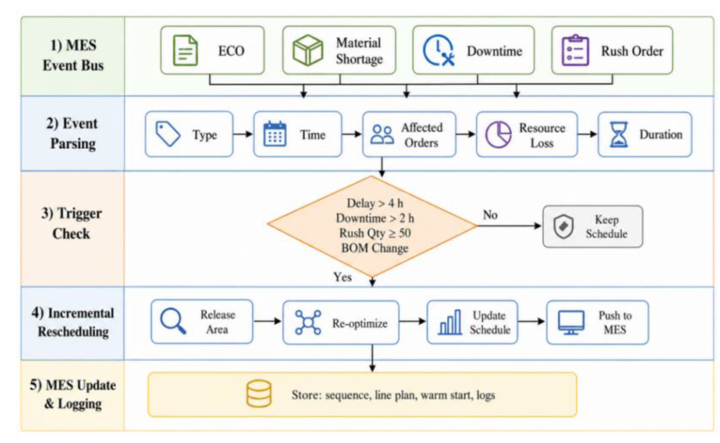
Figure 3.
Scheduling response surface and capacity transfer characteristics under multi-disturbance coupling.
Figure 3.
Scheduling response surface and capacity transfer characteristics under multi-disturbance coupling.
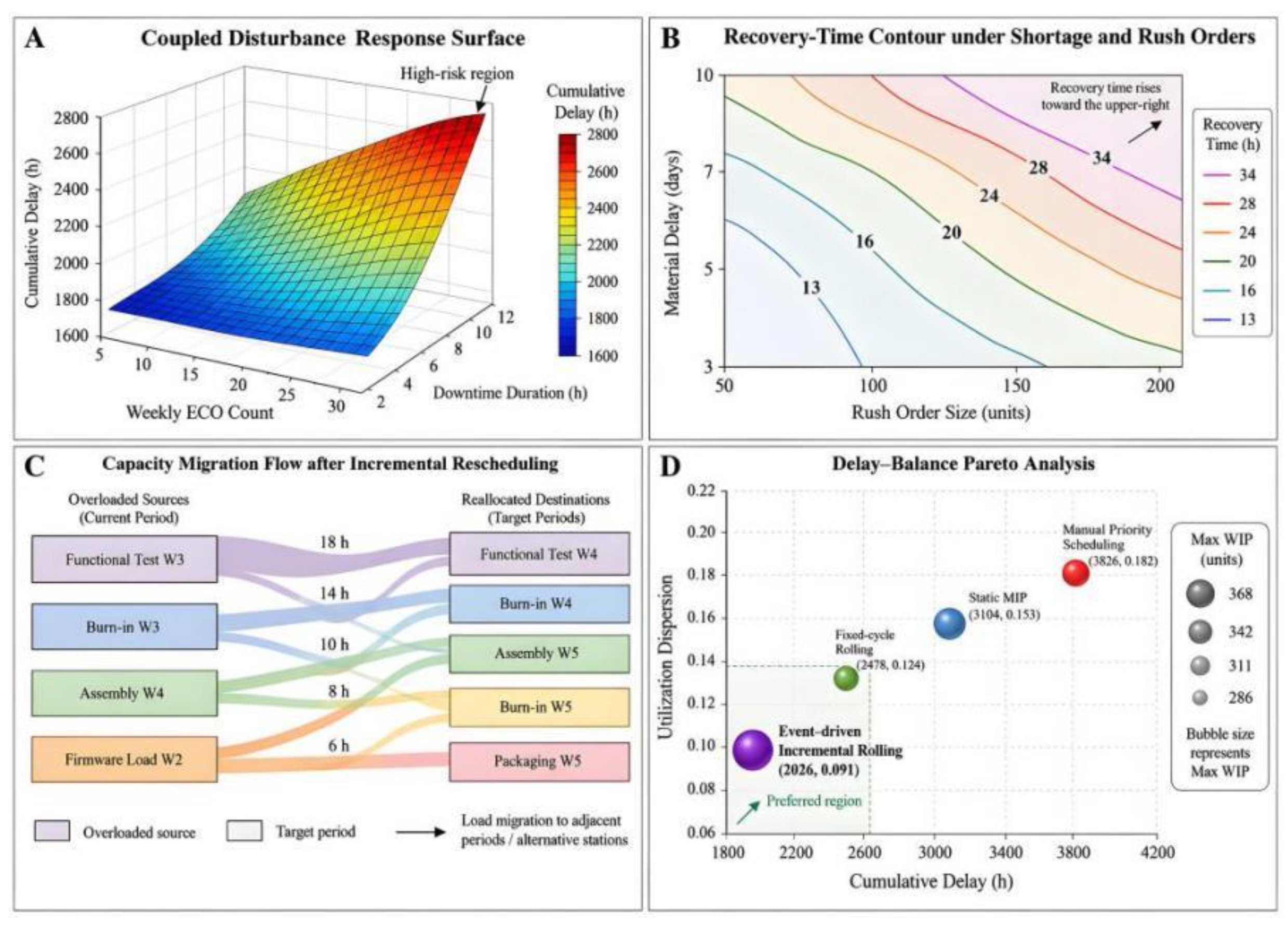
Figure 4.
Adaptive neighborhood expansion and scheduling recovery evolution under composite disturbances.
Figure 4.
Adaptive neighborhood expansion and scheduling recovery evolution under composite disturbances.
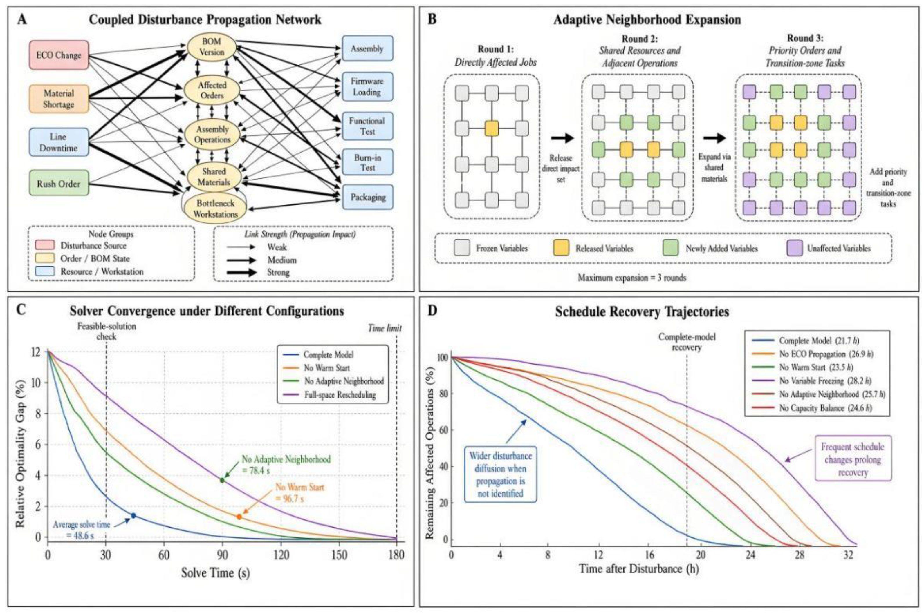
Table 2.
Algorithm Stability and Module Ablation Results.
| Model Configuration | Cumulative Delay / h | Average Solution Time / s | Rescheduling Event Count | Recovery Time / h | Utilization Dispersion |
| Full Model | 2026 ± 94 (2001.7–2050.3) | 48.6 ± 4.1 (47.5–49.7) | 61 ± 4 (60.0–62.0) | 21.7 ± 1.4 (21.3–22.1) | 0.091 ± 0.006 (0.089–0.093) |
| Remove ECO Effect Propagation | 2248 ± 108 (2220.1–2275.9) | 54.2 ± 4.8 (53.0–55.4) | 70 ± 5 (68.7–71.3) | 26.9 ± 1.8 (26.4–27.4) | 0.106 ± 0.008 (0.104–0.108) |
| Remove Warm Start | 2089 ± 99 (2063.4–2114.6) | 96.7 ± 8.6 (94.5–98.9) | 63 ± 4 (62.0–64.0) | 23.5 ± 1.6 (23.1–23.9) | 0.094 ± 0.007 (0.092–0.096) |
| Remove Variable Freezing | 1987 ± 92 (1963.2–2010.8) | 51.3 ± 4.5 (50.1–52.5) | 104 ± 7 (102.2–105.8) | 28.2 ± 2.0 (27.7–28.7) | 0.088 ± 0.006 (0.086–0.090) |
| Remove Adaptive Neighborhood | 2196 ± 105 (2168.9–2223.1) | 78.4 ± 6.9 (76.6–80.2) | 76 ± 5 (74.7–77.3) | 25.7 ± 1.7 (25.3–26.1) | 0.112 ± 0.009 (0.110–0.114) |
| Remove Capacity Balancing Term | 2114 ± 101 (2087.9–2140.1) | 45.8 ± 3.9 (44.8–46.8) | 66 ± 4 (65.0–67.0) | 24.6 ± 1.6 (24.2–25.0) | 0.156 ± 0.011 (0.153–0.159) |
Disclaimer/Publisher’s Note: The statements, opinions and data contained in all publications are solely those of the individual author(s) and contributor(s) and not of MDPI and/or the editor(s). MDPI and/or the editor(s) disclaim responsibility for any injury to people or property resulting from any ideas, methods, instructions or products referred to in the content. |
© 2026 by the authors. Licensee MDPI, Basel, Switzerland. This article is an open access article distributed under the terms and conditions of the Creative Commons Attribution (CC BY) license.
Copyright: This open access article is published under a Creative Commons CC BY 4.0 license, which permit the free download, distribution, and reuse, provided that the author and preprint are cited in any reuse.