Nodal Filters in Equality Algebras

1. Introduction

It is well known that order-theoretic and lattice-theoretic methods play a central role in algebraic logic [2,10,19,20]. Structures such as residuated lattices provide a natural semantic environment for substructural and fuzzy logics. Among the most influential related systems are BL-algebras and MV-algebras. MV-algebras, introduced by Chang in 1958 [6], serve as an algebraic semantics for Łukasiewicz infinite-valued propositional logic; notably, Chang established the algebraic completeness theorem for this logic. These developments significantly shaped the modern theory of algebraic semantics for non-classical logics. Heyting algebras, introduced by Arend Heyting [8], provide an algebraic framework for intuitionistic logic. Heyting algebras constitute one of the fundamental ordered structures in constructive logic and have inspired numerous generalizations. EQ-algebras were introduced by Novák and De Baets in [15] as abstract structures capturing essential logical operations. Subsequently, Jenei (2012) [9] defined the notion of equality algebras as a structurally simpler and more tractable system closely related to EQ-algebras and residuated structures [10].

In 2018, Borzooei [3] initiated a systematic study of various types of filters in equality algebras [2,19]. Later, in 2025, Zahedi and Hadinejad [7] examined certain classes of filters in equality algebras. Equality algebras have attracted increasing attention due to their suitability for studying logical equivalence and related algebraic phenomena [19]. Equality algebras were introduced as an algebraic framework for capturing the logical notion of equality in non-classical logics, particularly in the context of fuzzy logic and set theory. These algebras are endowed with a meet operation and an equality operation, which together induce an implication connective, thereby providing a natural setting for studying entailment and equivalence relations within a unified structure. A central theme in the theory of equality algebras is the study of filters [3,20], which serve as analogues of deductive systems and play a crucial role in characterizing consistency, maximality, and completeness. However, not all filters exhibit the same structural behavior, and it is often necessary to isolate those with special properties that reflect deeper algebraic or logical regularities [1,4,5,11,12,13,14,16,17].

Among such classes, the notion of a nodal filter has recently gained attention through the work of Xun and Xin [18]. A filter is called nodal (of type 1) if it is a node in the poset of all filters ordered by inclusion, that is, if it is comparable with every other filter. This seemingly simple order-theoretic condition imposes strong rigidity on the filter lattice and makes nodal filters natural candidates for serving as reference points, or “skeletons,” within the filter structure.

The necessity of investigating nodal filters arises from several interrelated considerations:

1.

Structural analysis of the filter poset. Since the set of all filters of an equality algebra forms a partially ordered set, identifying its nodes provides insight into the global organization of the filter system. Nodes act as elements that partition or orient the poset, and their classification contributes to a complete understanding of the filter lattice.

2.

Connections to well-known filter classes. Recent results have established that positive implicative filters are always nodal filters of type 1 (Theorem 3.14). The converse, however, fails in general, as demonstrated by a concrete counterexample (Example 3.15). This indicates that nodal filters form a strictly broader and more flexible class, one that can unify and generalize various implicative-type filters studied in the literature.

3.

Behavior in dense equality algebras. In dense equality algebras – where every nonzero element is dense – the situation becomes particularly tractable. It is shown (Theorem 3.17) that every implicative filter is necessarily nodal of type 1. This result highlights the relevance of nodal filters in special subclasses and suggests that density conditions simplify the comparability structure of filters.

4.

Logical and model-theoretic implications. Given the deep connections between equality algebras and logical systems (such as fuzzy logics and intuitionistic-type systems), nodal filters can be employed to define maximal theories, characterize conservative extensions, or construct canonical models. Their comparability property makes them ideal for situations in which one seeks filters that are either minimal over certain conditions or maximal under others.

In light of these motivations, the present work undertakes a systematic study of nodal filters in equality algebras, and the results obtained are briefly summarized in the abstract.

2. Preliminaries

In this section, we recall several definitions and known results that will be used throughout the paper.

Definition 1

([9]). An algebraic structure $(E,\wedge ,\sim ,1)$ of type $(2,2,0)$ is called an equality algebra if the following conditions hold for all $x,y,z\in E$ :

(E1) $(E,\wedge ,1)$ is a commutative idempotent integral monoid; equivalently, it is a meet semilattice with the greatest element 1,

(E2) $x\sim y=y\sim x$,

(E3) $x\sim x=1$,

(E4) $x\sim 1=x$,

(E5) If $x\le y\le z$, then $x\sim z\le y\sim z$ and $x\sim z\le x\sim y$,

(E6) $x\sim y\le (x\wedge y)\sim (y\wedge z)$,

(E7) $x\sim y\le (x\sim z)\sim (y\sim z)$.

The operation ∧ is called the meet (or infimum) operation, while the operation ∼ is called the equality operation.

The partial order ≤ on E is defined by

$$x\le y\mathrm{if}\mathrm{and}\mathrm{only}\mathrm{if}x\wedge y=x,\mathrm{for}\mathrm{all}x,y\in E.$$

On every equality algebra, the binary operations → and ↔ , called the implication and equivalence operations, respectively, are defined by:

$$x\to y=x\sim (x\wedge y),$$

$$x\leftrightarrow y=(x\to y)\wedge (y\to x).$$

An equality algebra is called equivalential if the equality operation ∼ coincides with the equivalence operation ↔ .

Throughout the paper, unless otherwise stated, E denotes an equality algebra.

Definition 2

([9]). We say that E is:

1. Bounded if there exists an element $0\in E$ such that $0\le x$ for all $x\in E$, also, in a bounded equality algebra, the negation operation′ is defined by

$$x^{\prime }=x\to 0=x\sim 0,\mathit{for}\mathit{all}x\in E.$$

2. Involutive if it is bounded and

$${\left(x^{\prime }\right)}^{\prime }=x,\mathit{for}\mathit{all}x\in E.$$

3. Pre-linear if, for all $x,y\in E$, the element 1 is the unique bounded E is called of the set $\{x\to y,y\to x\}$.

4. Commutative if, for all $x,y\in E$:

$$(x\to y)\to y=(y\to x)\to x.$$

5. A lattice equality algebra if it also a lattice.

6. Stonean if it is bounded and

$$x^{\prime }\vee x^{″}=1\mathit{for}\mathit{all}x\in E,\mathit{where}{x}^{″}={\left(x^{\prime }\right)}^{\prime }.$$

The following properties are well- known and will be used in the sequel.

Proposition 1

([9]). Let $(E,\wedge ,\sim ,1)$ be an equality algebra. Then the following statements hold for all $x,y,z\in E$:

(i) $x\sim y\le x\leftrightarrow y\le x\to y$,

(ii) $x\le (x\sim y)\sim y$,

(iii) $x\sim y=1\iff x=y$,

(iv) $x\to y=1\iff x\le y$,

(v) If $x\to y=1$ and $y\to x=1$, then $x=y$,

(vi) $1\to x=x,x\to 1=1,x\to x=1$,

(vii) $x\le y\to x,x\to (y\to x)=1$,

(viii) $x\le (x\to y)\to y,x\to \left(\right(x\to y)\to y)=1$,

(ix) $x\to y\le (y\to z)\to (x\to z),(x\to y)\to \left(\right(y\to z)\to (x\to z\left)\right)=1$,

(x) $\le y\to z\iff y\le x\to z$,

(xi) $x\to (y\to z)=y\to (x\to z)$,

(xii) $x\leftrightarrow x=1,x\leftrightarrow 1=x$,

(xiii) If $y\le x$, then $x\leftrightarrow y=x\to y=x\sim y$,

(xiv) If $x\le y$, then $y\to z\le x\to z,z\to x\le z\to y$,

(xv) $x\to y=x\to (x\wedge y)$,

(xvi) $x\sim y\le (z\to x)\sim (z\to y)$,

(xvii) $x\sim y\le (z\to x)\to (z\to y)$,

(xviii) $x\to y\le (z\to x)\to (z\to y)$,

(xix) $x\to y\le (x\wedge z)\to (y\wedge z)$,

(xx) $x\to y=\left(\right(x\to y)\to y)\to y$.

Proposition 2

([20]). Let E be a lattice equality algebra. Then, for all $x,y,z\in E$, the following statements hold: (i) $x\to y=(x\vee y)\to y$, (ii) $(x\vee y)\to z=(x\to z)\wedge (y\to z)$.

Proposition 3

([20]). Let E be a bounded lattice equality algebra. Then, for all $x,y\in E$, the following statements hold: (i) $x\le x^{″}$, (ii) ${(x\vee y)}^{\prime }=x^{\prime }\wedge y^{\prime }$.

Theorem 1

([20]). Every commutative equality algebra is a lattice.

Theorem 2

([20]). Any pre- linear equality algebra is a distributive lattice.

Definition 3

([10]). Let F be a non- empty subset of E. Then F is called a filter of E if, for all $x,y\in E$, the following conditions hold: (i) $1\in F$, (ii) if $x\in F$ and $x\le y$, then $y\in F$, (iii) if $x\in F$ and $x\sim y\in F$, then $y\in F$.

Denote by $F\left(E\right)$ the set of all filters of E. It is clear that $F\left(E\right)$ is closed under arbitrary intersections and that $\left\{1\right\}\in F\left(E\right)$.

A filter F of E is called proper if $F\ne E$. If E is a bounded equality algebra, then a filter F is proper if and only if $0\notin F$.

A proper filter F of E is called maximal if it is not contained in any other proper filter of E.

Proposition 4

([9]). $F\in F\left(E\right)$ if and only if for all $x,y\in E$ (i) $1\in F$, (ii) if $x\in F$ and $x\to y\in F$, then $y\in F$.

Proposition 5

([3]). Let F be a filter of E. Then F is a sub- algebra of E.

Proposition 6

([3]). Let F be a filter of E. Then $x\to y$, $x\sim y$, $x\wedge y\in F$ for all $x,y\in F$.

Theorem 3

([19]). Let X be a subset of an equality algebra E. Then the following statements hold: (i) The filter generated by X, denoted by $\langle X\rangle$, is given by

$$\langle X\rangle =\{a\in E\mid \mathit{there}\mathit{exist}n\in \mathbb{N}\mathit{and}{x}_1,\dots ,x_n\in X\mathit{such}\mathit{that}{x}_1\to (x_2\to \dots (x_n\to a)\dots )=1\}.$$

(ii) If D is a filter of E and $S\subseteq E$, then

$$\langle D\cup S\rangle =\{a\in E\mid \mathit{there}\mathit{exist}n\in \mathbb{N}\mathit{and}{s}_1,\dots ,s_n\in S\mathit{such}\mathit{that}{s}_1\to (s_2\to \dots (s_n\to a)\dots )\in D\}.$$

For each $x\in E$, the filter generated by $\left\{x\right\}$ is called a principal filter. Clearly,

$$\langle x\rangle =\{a\in E\mid x{\to }_{n}a=1,\mathit{for}\mathit{some}n\in \mathbb{N}\},$$

where the iterated implication is defined by

$$x{\to }_{0}a=a,x{\to }_{n}a=x\to \left(x{\to }_{n-1}a\right),n\ge 1.$$

Remark 1

([3]). Let $F,G\in F\left(E\right)$. Then define:

$$F\wedge G=F\cap G\mathit{and}F\vee G=\langle F\cup G\rangle .$$

Definition 4

([3]). Let F be a subset of E and $1\in F$. Then we say that F is:

(i) A positive implicative filter of E if:

$$x\to (y\to z)\in F\mathit{and}x\to y\in F\mathit{imply}(x\to z)\in F.$$

(ii) An implicative filter of E if:

$$z\to \left(\right(x\to y)\to x)\in F\mathit{and}z\in F\mathit{imply}x\in F.$$

(iii) A fantastic filter of E if:

$$z\to (y\to x)\in F\mathit{and}z\in F\mathit{imply}\left(\right(x\to y)\to y)\to x\in F.$$

for all $x,y,z\in E$.

Proposition 7

([3]). Let F be a filter of E. Then F is a positive implicative filter if and only if, for all $x,y,z\in E$:

$$(x\wedge (x\to y\left)\right)\to y\in F.$$

Proposition 8

([3]). Let F be a filter of a bounded equality algebra E. Then F is an implicative filter if and only if, for all $x\in E$:

$$(x^{\prime }\to x)\to x\in F.$$

Proposition 9

([3]). Let F be a filter of a bounded equality algebra E. Then for all $x,y,z\in E$, the following statements are equivalent: (i) F is an implicative filter of E. (ii) If $(x\to y)\to x\in F$, then $x\in F$. (iii) If $x^{\prime }\to x\in F$, then $x\in F$.

Proposition 10

([3]). Let F be a filter of E. Then the following conditions are equivalent: (i) F is a fantastic filter of E, (ii) $y\to x\in F$ implies $\left(\right(x\to y)\to y)\to x\in F$, for all $x,y\in E$, (iii) If E is a lattice, then $\left(\right(x\to y)\to y)\to \left(\right(y\to x)\to x)\in F$, for all $x,y\in E$.

Definition 5

([3]). Let E be a bounded lattice equality algebra. A filter F of E is called a Boolean filter if $x\vee x^{\prime }\in F$, for all $x\in E$.

Theorem 4

([3]). Let F be a proper filter of a pre- linear equality algebra E. Then the following statements are equivalent: F is a prime filter: (i) F is a prime filter, (ii) for each $x,y\in E$, if $x\vee y\in F$, then $x\in F$ or $y\in F$.

Definition 6

([7]). Let E be a bounded lattice equality algebra. A filter F of E is called a Stonean filter if $x^{\prime }\vee x^{″}\in F$, for all $x\in E$.

Definition 7

([2]). Let $(L,\vee ,\wedge ,\prime ,0,1)$ be a bounded lattice of type $(2,2,1,0,0)$. Then: (i) L is called a Kleene algebra if $x\wedge x^{\prime }\le y\vee y^{\prime }$, for all $x,y\in L$. (ii) L is called a semi-De Morgan algebra if $(L,\vee ,\wedge ,0,1)$ is a distributive lattice, with $0^{\prime }=1$, $1^{\prime }=0$, and for all $x,y\in L$:

$${(x\vee y)}^{\prime }=x^{\prime }\wedge y^{\prime },{(x\wedge y)}^{″}=x^{″}\wedge y^{″}\mathit{and}{x}^{‴}=x^{\prime }.$$

3. Some Types of Nodal Filters in Equality Algebras

3.1. Nodes in Equality Algebras

In this section, we introduce the concept of nodes in equality algebras and investigate some of their fundamental properties. We also study the relationship between nodes and other distinguished elements of equality algebras.

Definition 8.

Let $(P,\le )$ be a partially ordered set. An element $a\in P$ is called a node if, for every $x\in P$, either $x\le a$ or $a\le x$.

Since every equality algebra is naturally equipped with a partial order, the notion of a node can be defined analogously for equality algebras. We denote by $N\left(E\right)$ the set of all nodes of an equality algebra E.

Clearly,

$$1\in N\left(E\right).$$

Hence,

$$N\left(E\right)\ne ⌀.$$

Note. If E is a chain (that is, a totally ordered set), then every element of E is a node. Consequently,

$$N\left(E\right)=E.$$

Definition 9.

Let E be a bounded equality algebra with least element 0 and greatest element 1.

1.

An element $0\ne x\in E$ is called dense if

$$x^{\prime }=x\to 0=x\sim 0=0.$$

2.

An element $x\in E$ is called regular if

$$x^{″}=x.$$

3.

An element $x\in E$ is called a co-atom if it is a maximal element of $E\setminus \left\{1\right\}$. Dually, x is called an atom if it is a minimal element of $E\setminus \left\{0\right\}$.

In the following examples, we demonstrate that the notion of a node is, in general, independent of other distinguished classes of elements in equality algebras, including regular elements, atoms, co-atoms, and dense elements.

Example 1.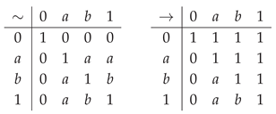

Let $E=\{0,a,b,1\}$ be a chain, as shown in the diagram below. Let us assume that $E=\{0,a,b,1\}$ is a chain such that $0\le a\le b\le 1$.

Figure 1.

Figure 1.

Define the operations ∼ (equality) and → (implication) as follows:

Then $(E,\wedge ,\sim ,1)$ is an equality algebra [3], and since E is a chain, all elements are nodes. Thus, $N\left(E\right)=\{0,a,b,1\}$, and moreover $F\left(E\right)=\left\{\right\{1\},\{b,1\},\{0,a,b,1\left\}\right\}$. Specifically, some of its distinct subsets are as follows:

Nodes: $N\left(E\right)=\{0,a,b,1\}$,

Atoms:$Atoms\left(E\right)=\left\{a\right\}$,

Co-atoms:$Co-atoms\left(E\right)=\left\{b\right\}$,

Dense elements:$Dense\left(E\right)=\{a,b,1\}$,

Regular elements:$Regular\left(E\right)=\left\{1\right\}$.

This example shows that node sets are generally distinct from atom sets, co-atom sets, dense sets, and regular set elements in equality algebras.

Example 2.

Let $E=\{0,a,b,c,d,1\}$ and $(E,\le )$ be a lattice whose Hasse diagram is below:

Figure 2.

Figure 2.

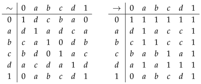
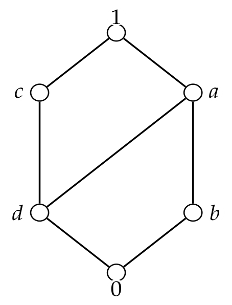
Define the operations ∼ (equality) and → (implication) as follows:

Then $(E,\wedge ,\sim ,1)$ is an equality algebra [3], specifically, some of its distinct subsets are as follows:

Nodes:  $N\left(E\right)=\{0,1\}$,

Atoms:  $Atoms\left(E\right)=\{b,d\}$,

Co-atoms:  $Co-atoms\left(E\right)=\{a,c\}$,

Dense elements: $Dense\left(E\right)=\left\{1\right\}$,

Regular elements: $Regular\left(E\right)=\{0,a,b,c,d,1\}$.

This example shows that the node set is generally distinct from the atoms set, co-atoms set, dense set, and regular set elements in equality algebras.

Example 3.

Let $E=\{0,a,b,c,d,1\}$ and $(E,\le )$ be a lattice whose Hasse diagram is below:

Figure 3.

Figure 3.

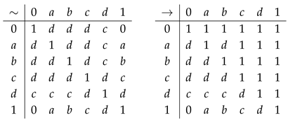
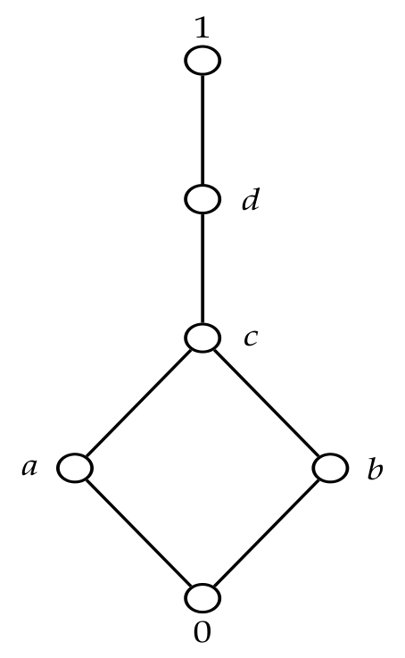
Define the operations ∼ (equality) and → (implication) as follows:

Then $(E,\wedge ,\sim ,1)$ is an equality algebra [3], specifically, some of its distinct subsets are as follows:

Nodes: $N\left(E\right)=\{0,c,d,1\}$,

Atoms: $Atoms\left(E\right)=\{a,b\}$,

Co-atoms: $Co-atoms\left(E\right)=\left\{d\right\}$,

Dense elements: $Dense\left(E\right)=\left\{1\right\}$,

Regular elements: $Regular\left(E\right)=\{0,c,d,1\}$.

It is clear that $N\left(E\right)=\{0,c,d,1\}$. The elements $a,b$ are atoms, but they are not nodes. And the elements $0,c,d,1$ are regular.

In addition, $F\left(E\right)=\left\{\right\{1\},\{c,1\},\{c,d,1\},\{a,b,c,d,1\},E\}$.

3.2. Nodal Filters in Equality Algebras

Definition 10.

Let E be an equality algebra and let F be a filter of E. We call F anodal filterof:

(i)

type 1 if F is a node in the partially ordered set

$$\left(F\right(E),\subseteq );$$

(ii)

type 2 if every element of F is a node of E;

(iii)

type 3 if the elements of F are pairwise comparable in E; that is, for all $a,b\in F$, either

$$a\le b\mathit{or}b\le a.$$

We denote by ${\mathrm{NF}}_1\left(E\right)$, ${\mathrm{NF}}_2\left(E\right)$, and ${\mathrm{NF}}_3\left(E\right)$ the sets of nodal filters of type 1, type 2, and type 3 in E, respectively. Unless otherwise stated, a nodal filter is assumed to be of type 1.

Remark 2.

If E is a chain, then the notions of nodal filters of types 1, 2, and 3 coincide.

Example 4.

Let $E=\{0,a,b,1\}$ be as in Example 1. Then all filters are nodal of types 1, 2 and 3, because $F\left(E\right)=\left\{\right\{1\},\{b,1\},\{0,a,b,1\left\}\right\}$. Thus:

$$F\left(E\right)={\mathrm{NF}}_1\left(E\right)={\mathrm{NF}}_2\left(E\right)={\mathrm{NF}}_3\left(E\right).$$

Note. In general, nodal filters of type 1, 2, and 3 have no relationship with each other.

Example 5.

Let $E=\{0,a,b,c,1\}$ and $(E,\le )$ be a lattice with the following Hasse diagram:

Figure 4.

Figure 4.

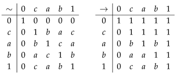
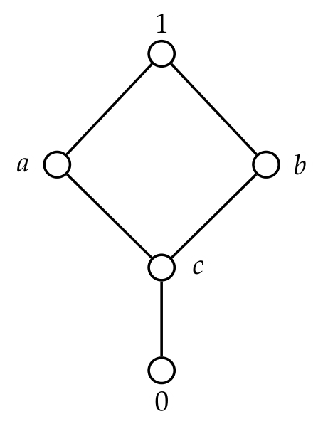
Define the operations ∼ (equality) and → (implication) by the following tables:

Then $(E,\wedge ,\sim ,1)$ is an equality algebra [3], and $F\left(E\right)=\left\{\right\{1\},\{a,1\},\{b,1\},\{a,b,c,1\},E\}$. Its nodal filters of different types are:

$${\mathrm{NF}}_1\left(E\right)=\{\left\{1\right\},\{a,b,c,1\},E\},$$

$${\mathrm{NF}}_2\left(E\right)=\left\{\left\{1\right\}\right\},$$

$${\mathrm{NF}}_3\left(E\right)=\{\left\{1\right\},\{a,1\},\{b,1\}\}.$$

It is observed that: ${\mathrm{NF}}_1\left(E\right)\ne {\mathrm{NF}}_2\left(E\right)\ne {\mathrm{NF}}_3\left(E\right)$ and ${\mathrm{NF}}_2\left(E\right)\subset {\mathrm{NF}}_3\left(E\right)$.

Remark 3.(i) Every nodal filter of type 2 is a nodal filter of type 3. However, the converse does not hold in general, as shown by Example 5. Moreover, this example also shows that, in general, a nodal filter need not be a prime filter. To see this, consider $F=\left\{1\right\}$. Then F is a nodal filter of type 1, 2, and 3. However, F is not a prime filter, since there exist $a,b\in E$ such that $a\vee b=1$, while $a\notin F$ and $b\notin F$, by Theorem 4.

(ii) Let $F,G\in {\mathrm{NF}}_3\left(E\right)$ and define $F\wedge G=F\cap G$ (cf. Remark 1). Then clearly $F\wedge G\in {\mathrm{NF}}_3\left(E\right)$. Hence, $({\mathrm{NF}}_3\left(E\right),\wedge )$ forms a meet-semilattice.

(iii) In general, $({\mathrm{NF}}_3\left(E\right),\vee )$ does not form a join-semilattice. Indeed, in Example 5, let $F=\{a,1\}$ and $G=\{b,1\}$ be nodal filters of type 3. Then

$$F\vee G=\langle \{a,1\}\cup \{b,1\}\rangle =\{a,b,c,1\},$$

which is not a nodal filter of type 3.

Theorem 5.

Let x be a node in E. Then the principal filter $\langle x\rangle$ is a nodal filter of type 1.

Proof. 

Let $x\in E$ be a node and consider the principal filter $\langle x\rangle$. We show that $\langle x\rangle$ is a node in the poset $\left(F\right(E),\subseteq )$. Let F be any filter of E. We consider two cases.

If $x\in F$, then by definition of the principal filter, we have

$$\langle x\rangle \subseteq F.$$

Assume now that $x\notin F$. Suppose that $F\subseteq \langle x\rangle$. Then there exists $y\in F$ such that $y\notin \langle x\rangle$, i.e., $x\le y$. Since x is a node in E, for every $y\in E$ we have either $x\le y$ or $y\le x$. From $x\le y$, it follows that $y\le x$. Hence, $y\in \langle x\rangle$, which implies $F\subseteq \langle x\rangle$, a contradiction.

Therefore, for every filter F, either

$$\langle x\rangle \subseteq F$$

or

$$F\subseteq \langle x\rangle .$$

Hence, $\langle x\rangle$ is a node in $\left(F\right(E),\subseteq )$, and so it is a nodal filter of type 1. □

Proposition 11.

Let E be an equality algebra and let $F\in {\mathrm{NF}}_3\left(E\right)$. Then $(F,\wedge ,\vee ,1)$ is a distributive lattice.

Proof. 

Since $F\in {\mathrm{NF}}_3\left(E\right)$, any two elements of F are comparable with respect to the order ≤. Hence, $(F,\le )$ is a chain. Therefore, for every $a,b\in F$, the elements

$$a\wedge b=min\{a,b\},a\vee b=max\{a,b\},$$

exist in F. Thus, $(F,\wedge ,\vee )$ is a lattice. Since every chain is distributive, the distributive laws

$$a\wedge (b\vee c)=(a\wedge b)\vee (a\wedge c),$$

and

$$a\vee (b\wedge c)=(a\vee b)\wedge (a\vee c),$$

hold for all $a,b,c\in F$. Hence, $(F,\wedge ,\vee ,1)$ is a distributive lattice. □

The following example shows that the converse of Proposition 11 does not hold in general.

Example 6.

Consider the equality algebra E of Example 5. Take $F=\{a,b,c,1\}\in {\mathrm{NF}}_1\left(E\right)$. Then $(F,\vee ,\wedge ,1)$ forms a distributive lattice. However, F is not a chain, since $a\le b$ and $b\le a$. Therefore, F is not a nodal filter of type 3.

Theorem 6.

Every positive implicative filter of E is a nodal filter of type 1.

Proof. 

Let F be a positive implicative filter of E. Suppose, on the contrary, that F is not a nodal filter of type 1. Then there exists a filter $G\in F\left(E\right)$ such that neither $F\subseteq G$ nor $G\subseteq F$. Hence, there exist elements $x\in F\setminus G$ and $y\in G\setminus F$. Since F is a positive implicative filter, by Proposition 2.15 we have:

$$(x\wedge (x\to y\left)\right)\to y\in F.$$

(1)

Moreover, by the properties of meet and implication, we have $x\wedge (x\to y)\le x$ and $x\wedge (x\to y)\le x\to y$. Which implies:

$$x\to y\le (x\wedge (x\to y\left)\right)\to y.$$

(2)

(Here we have used the inequality (xiv) of Proposition 2.3.)

We consider two cases:

Case 1: $x\to y\in F$. Since $x\in F$ and F is a filter (see Proposition 4), it follows that $y\in F$, which contradicts $y\notin F$.

Case 2: $x\to y\notin F$. Since $y\in G\setminus F$ and $y\le x\to y$ by Proposition 2.3 (vii), and since G is a filter (see Definition 2.8), we get $x\to y\in G$. Hence, $x\to y\in G\setminus F$. Using that G is a filter together with inequality (2), we conclude that $(x\wedge (x\to y\left)\right)\to y\in G\setminus F$, which contradicts (1), because $(x\wedge (x\to y\left)\right)\to y\in F$. Thus, in both cases we obtain a contradiction. Therefore, F is a nodal filter of type 1. □

The converse of Theorem 6 does not hold in general. That is, a nodal filter of type 1 is not necessarily a positive implicative filter. We present a concrete counterexample.

Example 7.

Let $E=\{0,a,b,1\}$ be a chain with the order $0\le a\le b\le 1$. Define the meet operation ∧ as the minimum. Define the equality operation ∼ as follows:

$$a\sim a=1,b\sim b=1,0\sim 0=1,$$

$$a\sim 1=1\sim a=a,b\sim 1=1\sim b=b,$$

$$0\sim a=a\sim 0=b,0\sim b=b\sim 0=a,$$

$$a\sim b=b\sim a=0.$$

One can verify that this satisfies all the axioms of an equality algebra (Definition 1). In this algebra, the implication is given by $x\to y=x\sim (x\wedge y)$.

The filters of E are exactly the upward-closed subsets containing 1, namely:

$$\left\{1\right\},\{b,1\},\{a,b,1\},E.$$

They form a chain under inclusion. Hence, every filter is a node in the poset $\left(F\right(E),\subseteq )$.

In particular, the filter $F=\left\{1\right\}$ is a nodal filter of type 1.

However, F is not a positive implicative filter. Indeed, take $x=a$ and $y=0$. Then

$$x\to y=a\to 0=a\sim 0=b,$$

$$x\wedge (x\to y)=a\wedge b=a.$$

Thus,

$$(x\wedge (x\to y\left)\right)\to y=a\to 0=b.$$

Since $b\ne 1$, we have $b\notin F=\left\{1\right\}$. Therefore, the filter F fails the positive implicative condition.

This shows that a nodal filter of type 1 need not be a positive implicative filter.

Definition 11.

An equality algebra E is called dense if every non-zero element of E is dense.

Theorem 7.

If E is a dense equality algebra, then every implicative filter of E is a nodal filter of type 1.

Proof. 

Let F be an implicative filter of E. Suppose, on the contrary, that F is not a nodal filter of type 1. Then there exists a filter $G\in F\left(E\right)$ such that neither $F\subseteq G$ nor $G\subseteq F$. Hence, there exist elements $x\in G\setminus F$ and $y\in F\setminus G$.

Since F is an implicative filter, by Proposition 8, we have

$$(x^{\prime }\to x)\to x\in F,$$

for all $x\in E$.

Since E is dense, every non-zero element is dense. In particular, for $x\ne 0$, we have $x^{\prime }=0$. Hence, by Proposition 1 (iv) and (vi), we have

$$(x^{\prime }\to x)\to x=(0\to x)\to x=1\to x=x.$$

Thus, $x\in F$, which contradicts $x\in G\setminus F$. Therefore, F must be comparable with every filter $G\in F\left(E\right)$, and hence F is a nodal filter of type 1. □

Note. The following example shows that the converse of Theorem 7 does not hold in general.

Example 8.

Consider the equality algebra E in Example 5. Let

$$F=\left\{1\right\}\in {\mathrm{NF}}_1\left(E\right).$$

Then F is not implicative. Indeed, taking $x=a$, by Proposition 1 (iv) and (vi), we have

$$(x^{\prime }\to x)\to x=(0\to a)\to a=1\to a=a\notin F.$$

Therefore, by Proposition 8, F is not implicative.

Theorem 8.

Let E be a pre-linear equality algebra. Then

$$\langle x\rangle \cup \langle y\rangle \subseteq \langle x\wedge y\rangle$$

for all $x,y\in E$.

Proof. 

Let

$$a\in \langle x\rangle \cup \langle y\rangle .$$

Then there exists $n\in \mathbb{N}$ such that

$$x{\to }_{n}a=1\mathrm{or}y{\to }_{n}a=1.$$

We first consider the case

$$x{\to }_{n}a=1.$$

We prove by induction on n that

$$x{\to }_{n}a\le (x\wedge y){\to }_{n}a.$$

Since

$$x\wedge y\le x,$$

by Proposition 1 (xiv), we have

$$x\to a\le (x\wedge y)\to a=(x\to a)\vee (y\to a).$$

(1)

Again, by Proposition 1 (xiv), (1) gives

$$x\to (x\to a)\le x\to \left(\right(x\wedge y)\to a).$$

(2)

Since $x\wedge y\le x$, another application of Proposition 1 (xiv) yields

$$x\to (x\to a)\le (x\wedge y)\to (x\to a).$$

(3)

Furthermore, by (1) and Proposition 1 (xiv), we obtain

$$(x\wedge y)\to (x\to a)\le (x\wedge y)\to \left(\right(x\wedge y)\to a).$$

(4)

Combining (3) and (4), we get

$$x\to (x\to a)\le (x\wedge y)\to \left(\right(x\wedge y)\to a).$$

(5)

Thus,

$$x{\to }_{2}a\le (x\wedge y){\to }_{2}a.$$

Continuing in the same way, suppose that

$$x{\to }_{n}a\le (x\wedge y){\to }_{n}a.$$

Since $x\wedge y\le x$, Proposition 1 (xiv) gives

$$x\to \left(x{\to }_{n}a\right)\le (x\wedge y)\to \left(x{\to }_{n}a\right),$$

and, using the induction hypothesis,

$$(x\wedge y)\to \left(x{\to }_{n}a\right)\le (x\wedge y)\to \left((x\wedge y){\to }_{n}a\right).$$

Hence,

$$x{\to }_{n+1}a\le (x\wedge y){\to }_{n+1}a.$$

Therefore, by induction,

$$x{\to }_{n}a\le (x\wedge y){\to }_{n}a$$

for every $n\in \mathbb{N}$.

Since $x{\to }_{n}a=1$, it follows that

$$1=x{\to }_{n}a\le (x\wedge y){\to }_{n}a.$$

Thus,

$$(x\wedge y){\to }_{n}a=1,$$

and consequently

$$a\in \langle x\wedge y\rangle .$$

Similarly, if

$$y{\to }_{n}a=1,$$

then the same argument, with x and y interchanged, gives

$$(x\wedge y){\to }_{n}a=1.$$

Hence,

$$a\in \langle x\wedge y\rangle .$$

Therefore,

$$\langle x\rangle \cup \langle y\rangle \subseteq \langle x\wedge y\rangle .$$

□

Note. The following example shows that the converse of Theorem 8 does not hold in general.

Example 9.

In Example 5, we have

$$\langle a\rangle =\{1,a\},\langle b\rangle =\{1,b\},$$

and

$$\langle a\wedge b\rangle =\langle c\rangle =\{a,b,c,1\}.$$

Hence,

$$\langle a\rangle \cup \langle b\rangle =\{1,a\}\cup \{1,b\}=\{1,a,b\},$$

while

$$\langle a\wedge b\rangle =\langle c\rangle =\{a,b,c,1\}.$$

Therefore,

$$\langle a\rangle \cup \langle b\rangle \subseteq \langle a\wedge b\rangle ,\langle a\wedge b\rangle \subseteq \langle a\rangle \cup \langle b\rangle .$$

Definition 12.

An equality algebra E is called a pure pre-linear equality algebra if

$$x\wedge y=x\sim y$$

for all distinct $x,y\in E$.

Definitio 13.

Let $F,G\in F\left(E\right)$. We define

$$F:G=\{x\in E\mid G\cap \langle x\rangle \subseteq F\}.$$

In particular, we define

$$F^{\prime }=\left\{1\right\}:F\mathrm{and}{G}^{\prime }=\left\{1\right\}:G.$$

Theorem 9.

If E is a pure pre-linear equality algebra, then for any $F,G\in F\left(E\right)$, we have $F:G\in F\left(E\right)$.

Proof. 

We verify that $F:G$ satisfies the three conditions of a filter.

(i) We first show that $1\in F:G$. Since

$$\langle 1\rangle =\left\{1\right\},$$

we have

$$G\cap \langle 1\rangle \subseteq F.$$

Thus, by Definition 13,

$$1\in F:G.$$

(ii) Suppose that $x\in F:G$ and $x\le y$. Then

$$\langle y\rangle \subseteq \langle x\rangle ,$$

and consequently,

$$G\cap \langle y\rangle \subseteq G\cap \langle x\rangle .$$

Since $x\in F:G$, we have

$$G\cap \langle x\rangle \subseteq F.$$

Therefore,

$$G\cap \langle y\rangle \subseteq F,$$

which implies, by Definition 13, that

$$y\in F:G.$$

(iii) Suppose that $x\in F:G$ and $x\sim y\in F:G$. By Definition 13,

$$G\cap \langle x\rangle \subseteq F\mathrm{and}G\cap \langle x\sim y\rangle \subseteq F.$$

Since E is a pure pre-linear equality algebra, by Definition 12, we have

$$x\wedge y=x\sim y.$$

Hence,

$$\langle x\wedge y\rangle =\langle x\sim y\rangle ,$$

and therefore

$$G\cap \langle x\wedge y\rangle \subseteq F.$$

Moreover, since

$$\langle x\rangle \cup \langle y\rangle \subseteq \langle x\wedge y\rangle ,$$

we obtain

$$G\cap \left(\langle x\rangle \cup \langle y\rangle \right)\subseteq G\cap \langle x\wedge y\rangle \subseteq F.$$

Thus,

$$(G\cap \langle x\rangle )\cup (G\cap \langle y\rangle )\subseteq F.$$

Since

$$G\cap \langle x\rangle \subseteq F,$$

it follows that

$$G\cap \langle y\rangle \subseteq F.$$

Hence, by Definition 13,

$$y\in F:G.$$

Therefore, $F:G$ satisfies all three filter conditions, and hence

$$F:G\in F\left(E\right).$$

□

Example 10.

Let $E=\{0,a,b,c,1\}$ and $(E,\le )$ be a lattice that diagram is below:

Figure 5.

Figure 5.

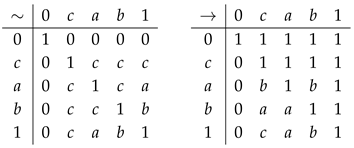
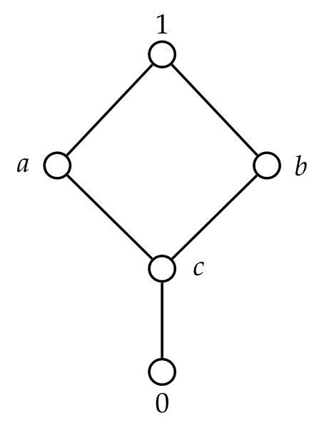
Define the operations ∼ (equality) and → (implication) as follows:

Then $(E,\wedge ,\sim ,1)$ is a pure pre- linear equality algebra. It is easy to check that:

$$F\left(E\right)=\left\{\right\{1\},\{a,1\},\{b,1\},\{a,b,c,1\},E\}.$$

The principal filters are: $\langle 1\rangle =\left\{1\right\}$, $\langle a\rangle =\{a,1\}$, $\langle b\rangle =\{b,1\}$, $\langle c\rangle =\{a,b,c,1\}$, $\langle 0\rangle =E$.

And its type 1, 2, and 3 nodal filters are as follows:

$${\mathrm{NF}}_1\left(E\right)=\{\left\{1\right\},\{a,b,c,1\},E\},$$

$${\mathrm{NF}}_2\left(E\right)=\left\{\left\{1\right\}\right\},$$

$${\mathrm{NF}}_3\left(E\right)=\{\left\{1\right\},\{a,1\},\{b,1\}\}.$$

$F:G$ for all filters, it will be as follows:

$F:G$	$F_1=\left\{1\right\}$	$F_2=\{a,1\}$	$F_3=\{b,1\}$	$F_4=\{a,b,c,1\}$	$F_5=E$
$F_1$	E	$\{b,1\}$	$\{a,1\}$	$\left\{1\right\}$	$\left\{1\right\}$
$F_2$	E	E	$\{a,1\}$	$\{a,1\}$	$\{a,1\}$
$F_3$	E	$\{b,1\}$	E	$\{b,1\}$	$\{b,1\}$
$F_4$	E	E	E	E	$\{a,b,c,1\}$
$F_5$	E	E	E	E	E

It can be seen that the result of $F:G$ is a filter.

Theorem 10.

Let E be a pure bounded pre-linear equality algebra and let $F,G\in F\left(E\right)$. If $F:G$ is a Boolean filter, then $F:G$ is a Stonean filter.

Proof. 

Since $F:G$ is a Boolean filter, by Definition 5, we have

$$x\vee x^{\prime }\in F:G$$

for every $x\in E$. By Definition 13, this implies

$$G\cap \langle x\vee x^{\prime }\rangle \subseteq F.$$

Since

$$x^{\prime }\le x^{\prime }\mathrm{and}x\le x^{″},$$

we have

$$x\vee x^{\prime }\le x^{\prime }\vee x^{″}.$$

Hence,

$$\langle x^{\prime }\vee x^{″}\rangle \subseteq \langle x\vee x^{\prime }\rangle .$$

Therefore,

$$G\cap \langle x^{\prime }\vee x^{″}\rangle \subseteq G\cap \langle x\vee x^{\prime }\rangle \subseteq F.$$

Thus,

$$G\cap \langle x^{\prime }\vee x^{″}\rangle \subseteq F.$$

By Definition 13, we obtain

$$x^{\prime }\vee x^{″}\in F:G$$

for every $x\in E$. Therefore, by Definition 6, $F:G$ is a Stonean filter. □

Note. The converse of Theorem 10 does not necessarily hold in general.

Example 11.

In Example 10, the Boolean filter is

$$\bigcup _{x\in E}\langle x\vee x^{\prime }\rangle =\{a,b,c,1\}.$$

Moreover, for every $x\in E$, we have

$$x^{\prime }\vee x^{″}=1.$$

Hence, every filter containing 1 is a Stonean filter. Thus, in this example, every Boolean filter is Stonean. However, the converse does not hold. For example, the filter

$$\{a,1\}$$

is Stonean, since it contains 1, but it is not Boolean, because

$$\{a,1\}\ne \{a,b,c,1\}.$$

Theorem 11.

Let E be a pure bounded pre-linear equality algebra and let $F,G\in F\left(E\right)$. If $F:G$ is a positive implicative filter, then $F:G$ is a Stonean filter.

Proof. 

Since $F:G$ is a positive implicative filter, by Proposition 7, we have

$$(x\wedge (x\to y\left)\right)\to y\in F:G$$

for all $x,y\in E$. Taking $y=0$, we obtain

$$(x\wedge (x\to 0\left)\right)\to 0\in F:G.$$

Since

$$x\to 0=x^{\prime },$$

it follows that

$$(x\wedge x^{\prime })\to 0\in F:G.$$

Moreover,

$$(x\wedge x^{\prime })\to 0={(x\wedge x^{\prime })}^{\prime }=x^{\prime }\vee x^{″}.$$

Therefore,

$$x^{\prime }\vee x^{″}\in F:G$$

for every $x\in E$.

By Definition 13, this means that

$$G\cap \langle x^{\prime }\vee x^{″}\rangle \subseteq F$$

for every $x\in E$. Hence,

$$x^{\prime }\vee x^{″}\in F:G$$

for all $x\in E$. Therefore, by Definition 6, $F:G$ is a Stonean filter. □

Note. The following example shows that the converse of Theorem 11 does not hold in general.

Example 12.

In Example 10, all filters are Stonean. However, the filter

$$\{b,1\}$$

is not a positive implicative filter.

Theorem 12.

If $F:G$ is an implicative filter, then $F:G$ is a fantastic filter.

Proof. 

Let $F:G$ be an implicative filter of E, and suppose that

$$y\to x\in F:G.$$

By Definition 13, we have

$$G\cap \langle y\to x\rangle \subseteq F.$$

Since

$$x\le \left(\right(x\to y)\to y)\to x,$$

by Proposition 1 (vii) and (xiv), we obtain

$$\left(\right((x\to y)\to y)\to x)\to y\le x\to y.$$

By Proposition 1 (xiv), applied to

$$\left(\right(x\to y)\to y)\to x,$$

we have

$$\begin{array}{cc}& \left(\right(\left(\right(x\to y)\to y)\to x)\to y)\to \left(\right((x\to y)\to y)\to x)\hfill \\ & \ge (x\to y)\to \left(\right((x\to y)\to y)\to x).\hfill \end{array}$$

(1)

By Proposition 1 (xi) and (xviii), together with (1), we obtain

$$\begin{array}{cc}\hfill (x\to y)\to \left(\right((x\to y)\to y)\to x)& =\left(\right(x\to y)\to y)\to \left(\right(x\to y)\to x)\hfill \\ & \ge y\to x.\hfill \end{array}$$

(2)

Combining (1) and (2), and applying Proposition 1 (xvii), we obtain

$$\begin{array}{cc}& \left(\right(\left(\right(x\to y)\to y)\to x)\to y)\to \left(\right((x\to y)\to y)\to x)\hfill \\ & \ge y\to x.\hfill \end{array}$$

Equivalently,

$$y\to x\le \left(\right(x\to y)\to y)\to \left(\right(x\to y)\to x).$$

Therefore,

$$〈\left(\right(x\to y)\to y)\to \left(\right(x\to y)\to x)〉\subseteq \langle y\to x\rangle .$$

Consequently,

$$\begin{array}{cc}\hfill G\cap 〈\left(\right(x\to y)\to y)\to \left(\right(x\to y)\to x)〉& \subseteq G\cap \langle y\to x\rangle \hfill \\ & \subseteq F.\hfill \end{array}$$

Thus, by Definition 13,

$$\left(\right(x\to y)\to y)\to \left(\right(x\to y)\to x)\in F:G.$$

By Proposition 9 (ii), it follows that

$$\left(\right(x\to y)\to y)\to x\in F:G.$$

Hence, by Proposition 10, $F:G$ is a fantastic filter. □

Theorem 13.

Let E be a dense equality algebra. Then every nodal filter of type 1, 2, or 3 is a Stonean filter, and conversely.

Proof. 

Suppose that E is a dense equality algebra and let F be a nodal filter of type 1, 2, or 3. We show that F is a Stonean filter.

For every $x\in E$, we consider two cases.

(1) If $x=0$, then

$$x^{\prime }\vee x^{″}=0^{\prime }\vee 0^{″}=1\vee 0=1\in F.$$

(2) If $x\ne 0$, since E is dense, we have $x^{\prime }=0$. Hence,

$$x^{\prime }\vee x^{″}=0\vee 0^{″}=0\vee 1=1\in F.$$

Thus, in both cases,

$$x^{\prime }\vee x^{″}\in F$$

for every $x\in E$. Therefore, by Definition 6, F is a Stonean filter.

The converse follows immediately from the definition. □

Note. The following example shows that the density assumption in Theorem 13 is essential.

Example 13.

The equality algebra in Example 3 is not dense. Moreover, $\left\{1\right\}$ is a nodal filter of types 1, 2, and 3, but it is not a Stonean filter. Indeed, taking $x=b$, we obtain

$$x^{\prime }\vee x^{″}=b^{\prime }\vee b^{″}=d\vee c=d.$$

Since

$$d\notin \left\{1\right\},$$

we conclude that

$$x^{\prime }\vee x^{″}\notin \left\{1\right\}.$$

Thus, $\left\{1\right\}$ is not a Stonean filter. Therefore, a nodal filter of type 1, 2, or 3 need not be a Stonean filter when the equality algebra is not dense.

Proposition 12.

Let E be an equality algebra. Then the following properties are satisfied, for all $F,G,H\in {\mathrm{NF}}_1\left(E\right)$:

(i) $E:F=E,F:F=E,F:E=E,F:\left\{1\right\}=E$,

(ii) If $F=\left\{1\right\}$, then $F^{\prime }=E,F^{″}=\left\{1\right\}$,

(iii) If $F\ne \left\{1\right\}$, then $F^{\prime }=\left\{1\right\},F^{″}=E$,

(iv) $F^{\prime }:G=G^{\prime }:F$ for $F,G\ne \left\{1\right\}$,

(v) $F\subseteq G$ implies $H:G\subseteq H:F$ and $F:H\subseteq G:H$,

(vi) $F\subseteq G\iff G:F=E$,

(vii) $F\subseteq F:G$,

(viii) $G\subseteq G:(G:F)$,

(ix) $G\subseteq (G:F):G$.

Proof. (i) By Definition 13, we have

$$E:F=\{x\in E\mid F\cap \langle x\rangle \subseteq E\}=E.$$

Moreover,

$$F:F=\{x\in E\mid F\cap \langle x\rangle \subseteq F\}=E,$$

since $F\cap \langle x\rangle \subseteq F$ for every $x\in E$. Thus,

$$E:F=F:F=E.$$

The proofs of the remaining cases are similar.

(ii) By (i) and Definition 13, we have

$$F^{\prime }=\left\{1\right\}:F=\left\{1\right\}:\left\{1\right\}=E.$$

Similarly,

$$F^{″}=\left\{1\right\}:F^{\prime }=\left\{1\right\}:E=\left\{1\right\}.$$

(iii) By Definition 13,

$$F^{\prime }=\left\{1\right\}:F=\{x\in E\mid F\cap \langle x\rangle \subseteq \left\{1\right\}\}.$$

Let $x\in E$ with $x\ne 1$. If $x\in F$, then

$$F\cap \langle x\rangle =\langle x\rangle \subseteq \left\{1\right\},$$

which is impossible.

On the other hand, suppose that $x\notin F$. Since F is a nodal filter of type 1, we have

$$F\subseteq \langle x\rangle .$$

Consequently,

$$F\cap \langle x\rangle =F\ne \left\{1\right\},$$

which is again impossible. Therefore, $x=1$, and hence

$$F^{\prime }=\left\{1\right\}:F=\left\{1\right\}.$$

Moreover, by (i),

$$F^{″}=\left\{1\right\}:F^{\prime }=\left\{1\right\}:\left\{1\right\}=E.$$

(iv) By (iii),

$$F^{\prime }=G^{\prime }=\left\{1\right\}.$$

Therefore,

$$G^{\prime }:F=\left\{1\right\}:F=F^{\prime }=\left\{1\right\}.$$

Similarly,

$$F^{\prime }:G=\left\{1\right\}.$$

Hence,

$$F^{\prime }:G=G^{\prime }:F.$$

(v) Suppose that $F\subseteq G$. If $x\in H:G$, then, by Definition 13,

$$G\cap \langle x\rangle \subseteq H.$$

Since $F\subseteq G$, we have

$$F\cap \langle x\rangle \subseteq G\cap \langle x\rangle \subseteq H.$$

Thus, $x\in H:F$, and therefore

$$H:G\subseteq H:F.$$

Similarly, if $F\subseteq G$ and $x\in F:H$, then

$$H\cap \langle x\rangle \subseteq F\subseteq G.$$

Hence, $x\in G:H$, and consequently

$$F:H\subseteq G:H.$$

(vi) Suppose, to the contrary, that $F\subseteq G$. Then there exists $x\in F$ such that $x\notin G$. Since $x\in F$, we have

$$\langle x\rangle \subseteq F,$$

and hence

$$F\cap \langle x\rangle =\langle x\rangle .$$

Since $x\notin G$, we have

$$\langle x\rangle \subseteq G,$$

which contradicts the definition of $G:F$. Therefore,

$$F\subseteq G.$$

Now, if $F\subseteq G$, then

$$F\cap \langle x\rangle \subseteq G\cap \langle x\rangle$$

for every $x\in E$. Hence, by Definition 13,

$$G:F=\{x\in E\mid G\cap \langle x\rangle \subseteq F\}=E.$$

(vii) This follows immediately from the definition of $F:G$.

(viii) By Definition 13,

$$G:(G:F)=\{x\in E\mid (G:F)\cap \langle x\rangle \subseteq G\}.$$

If $x\in F$, then, by the definition of $G:F$,

$$G\cap \langle x\rangle \subseteq F.$$

Therefore,

$$(G:F)\cap \langle x\rangle \subseteq G,$$

and hence $x\in G:(G:F)$. Thus,

$$F\subseteq G:(G:F).$$

(ix) By Definition 13,

$$(G:F):G=\{x\in E\mid G\cap \langle x\rangle \subseteq G:F\}.$$

If $x\in G$, then

$$\langle x\rangle \subseteq G$$

and, by the definition of $G:F$,

$$G\cap \langle x\rangle =\langle x\rangle \subseteq G:F.$$

Therefore, $x\in (G:F):G$. Hence,

$$G\subseteq (G:F):G.$$

□

Theorem 14.

Let E be an equality algebra and let $F,G\in {\mathrm{NF}}_1\left(E\right)$. Then

$$F:G\in {\mathrm{NF}}_1\left(E\right).$$

Proof. 

We show that $F:G$ is either E or F, both of which are nodal filters of type 1. Since ${\mathrm{NF}}_1\left(E\right)$ is pre-linear, we consider the following cases.

(i) Suppose that $F=G$. Then, by Proposition 12 (i),

$$F:G=F:F=E.$$

Hence,

$$F:G\in {\mathrm{NF}}_1\left(E\right).$$

(ii) Suppose that $F\ne G$.

(a) If $G\subseteq F$, then for every $x\in E$,

$$G\cap \langle x\rangle \subseteq G\subseteq F.$$

Therefore, by Definition 13,

$$F:G=E.$$

Hence,

$$F:G\in {\mathrm{NF}}_1\left(E\right).$$

(b) Suppose that $F\subseteq G$. We first prove that

$$F:G\subseteq F.$$

Let $x\in F:G$. By Definition 13,

$$G\cap \langle x\rangle \subseteq F.$$

If $x\in G$, then

$$G\cap \langle x\rangle =\langle x\rangle ,$$

and hence

$$\langle x\rangle \subseteq F.$$

Since F is a filter, it follows that $x\in F$.

Now suppose that $x\notin G$. Since G is a nodal filter of type 1, we have

$$G\subseteq \langle x\rangle .$$

Consequently,

$$G=G\cap \langle x\rangle \subseteq F.$$

Together with $F\subseteq G$, this gives

$$F=G,$$

which contradicts $F\ne G$. Therefore, $x\in G$, and hence $x\in F$. Thus,

$$F:G\subseteq F.$$

Conversely, let $x\in F$. Since $F\subseteq G$, we have $x\in G$, and because F is a filter,

$$\langle x\rangle \subseteq F.$$

Therefore,

$$G\cap \langle x\rangle =\langle x\rangle \subseteq F.$$

By Definition 13, we obtain

$$x\in F:G.$$

Hence,

$$F\subseteq F:G.$$

Therefore,

$$F:G=F.$$

Thus,

$$F:G\in {\mathrm{NF}}_1\left(E\right).$$

In all cases, $F:G$ is either E or F. Hence,

$$F:G\in {\mathrm{NF}}_1\left(E\right).$$

□

Note. It is clear from the Theorem 14, that if $F,G$ are two nodal filters of type 1, then $F:G$ is a nodal filter of type 1.

Example 14.

According to Example 5, we have:

$$F\left(E\right)=\left\{\right\{1\},\{a,1\},\{b,1\},\{a,b,c,1\},E\},$$

$$F_1=\left\{1\right\}=\langle 1\rangle ,$$

$$F_2=\{a,1\}=\langle a\rangle ,$$

$$F_3=\{b,1\}=\langle b\rangle ,$$

$$F_4=\{a,b,c,1\}=\langle c\rangle ,$$

$$F_5=E=\{0,a,b,c,1\}=\langle 0\rangle ,$$

${\mathrm{NF}}_1\left(E\right)=\{\left\{1\right\},\{a,b,c,1\},E\}$.

$F:G$	$F_1$	$F_2$	$F_3$	$F_4$	$F_5$
$F_1$	E	$\{b,1\}$	$\{a,1\}$	$\left\{1\right\}$	$\left\{1\right\}$
$F_2$	E	E	$\{a,1\}$	$\{a,1\}$	$\{a,1\}$
$F_3$	E	$\{a,b,1\}$	E	$\{a,b,1\}$	$\{b,1\}$
$F_4$	E	E	E	E	E
$F_5$	E	E	E	E	E

It is clear that if $F:G$ are not nodal filters of type 1, then $F:G$ will not be a nodal filter of type 1, as $F_2:F_4$, $F_2:F_3$.

Definition 14.

Let $F,G\in {\mathrm{NF}}_1\left(E\right)$. We define

$$F\wedge G=F\cap G$$

and

$$F\vee G=\langle F\cup G\rangle .$$

Theorem 15.$({\mathrm{NF}}_1\left(E\right),\vee ,\wedge )$ is a lattice.

Proof. (i) Let $H\in \mathcal{F}\left(E\right)$. If $F,G\subseteq H$, then

$$F\vee G=\langle F\cup G\rangle \subseteq H.$$

If $H\subseteq F,G$, then

$$H\subseteq \langle F\cup G\rangle =F\vee G.$$

Finally, if

$$F\subseteq H\subseteq G\mathrm{or}G\subseteq H\subseteq F,$$

then

$$H\subseteq \langle F\cup G\rangle =F\vee G.$$

Thus, in all cases, $F\vee G$ is a nodal filter of type 1. Hence,

$$F\vee G\in {\mathrm{NF}}_1\left(E\right).$$

(ii) Since ${\mathrm{NF}}_1\left(E\right)$ is pre-linear, either $F\subseteq G$ or $G\subseteq F$. If $F\subseteq G$, then

$$F\cap G=F\in {\mathrm{NF}}_1\left(E\right).$$

If $G\subseteq F$, then

$$F\cap G=G\in {\mathrm{NF}}_1\left(E\right).$$

Therefore, in either case,

$$F\wedge G=F\cap G\in {\mathrm{NF}}_1\left(E\right).$$

□

Theorem 16.$({\mathrm{NF}}_1\left(E\right),\vee ,\wedge )$ is a bounded distributive lattice.

Proof. 

By Theorem 15, $({\mathrm{NF}}_1\left(E\right),\vee ,\wedge )$ is a bounded lattice, whose smallest element is $\left\{1\right\}$ and whose largest element is E.

Now for all $F,G,H\in {\mathrm{NF}}_1\left(E\right)$, we prove:

$$F\wedge (G\vee H)=(F\wedge G)\vee (F\wedge H).$$

For this, we consider the following cases:

(1) $F\subseteq G\subseteq H$, then $F\cap \langle G\cup H\rangle =F\cap H=F=\langle F\cup F\rangle =\langle (F\cap G)\cup (F\cap H)\rangle$.

(2) $F\subseteq H\subseteq G$, then $F\cap \langle G\cup H\rangle =F\cap G=F=\langle F\cup F\rangle =\langle (F\cap G)\cup (F\cap H)\rangle$.

(3) $H\subseteq F\subseteq G$, then $F\cap \langle G\cup H\rangle =F\cap G=F=\langle F\cup H\rangle =\langle (F\cap G)\cup (F\cap H)\rangle$.

(4) $H\subseteq G\subseteq F$, then $F\cap \langle G\cup H\rangle =F\cap G=G=\langle G\cup H\rangle =\langle (F\cap G)\cup (F\cap H)\rangle$.

(5) $G\subseteq H\subseteq F$, then $F\cap \langle G\cup H\rangle =F\cap H=H=\langle G\cup H\rangle =\langle (F\cap G)\cup (F\cap H)\rangle$.

(6) $G\subseteq F\subseteq H$, then $F\cap \langle G\cup H\rangle =F\cap H=F=\langle G\cup H\rangle =\langle (F\cap G)\cup (F\cap H)\rangle$.

Therefore $({\mathrm{NF}}_1\left(E\right),\vee ,\wedge )$ is a bounded distributive lattice. □

Theorem 17.  $({\mathrm{NF}}_1\left(E\right),\vee ,\wedge ,\prime ,\left\{1\right\},E)$ is a Kleene algebra.

Proof. 

By Theorem refthm:3.37, $({\mathrm{NF}}_1\left(E\right),\vee ,\wedge )$ is a bounded distributive lattice.

For all $F,G\in {\mathrm{NF}}_1\left(E\right)$:

$$F\wedge F^{\prime }=F\wedge \left\{1\right\}=F\cap \left\{1\right\}=\left\{1\right\}\mathrm{and}G\vee G^{\prime }=G\vee \left\{1\right\}=\langle G\cup \left\{1\right\}\rangle$$

by Proposition 12 (iii).

It is clear that $\left\{1\right\}\subseteq \langle G\cup \left\{1\right\}\rangle$. Therefore, $({\mathrm{NF}}_1\left(E\right),\vee ,\wedge ,\prime ,\left\{1\right\},E)$ is a Kleene algebra, by Definition 7 (i). □

Theorem 18.$({\mathrm{NF}}_1\left(E\right),\vee ,\wedge ,\prime ,\left\{1\right\},E)$ is a semi-Demorgan algebra.

Proof. 

By Theorem 16,

$$({\mathrm{NF}}_1\left(E\right),\vee ,\wedge ,\left\{1\right\},E)$$

is a bounded distributive lattice. Let $F,G\in {\mathrm{NF}}_1\left(E\right)$. We prove that

$${(F\vee G)}^{\prime }=F^{\prime }\wedge G^{\prime },{(F\wedge G)}^{″}=F^{″}\wedge G^{″},F^{\prime }=F^{‴}.$$

We consider three cases.

(1) Suppose that $F=G=\left\{1\right\}$. Since $F^{\prime }=G^{\prime }=E$, we have

$$\begin{array}{cc}\hfill {(F\vee G)}^{\prime }& =\left\{1\right\}:\langle F\cup G\rangle \hfill \\ & =\left\{1\right\}:\left\{1\right\}\hfill \\ & =E\hfill \\ & =E\cap E\hfill \\ & =F^{\prime }\cap G^{\prime }=F^{\prime }\wedge G^{\prime }.\hfill \end{array}$$

Moreover,

$$\begin{array}{cc}\hfill {(F\wedge G)}^{″}& ={\left({(F\wedge G)}^{\prime }\right)}^{\prime }\hfill \\ & =E^{\prime }\hfill \\ & =\left\{1\right\}\hfill \\ & =\left\{1\right\}\cap \left\{1\right\}\hfill \\ & =F^{″}\cap G^{″}=F^{″}\wedge G^{″}.\hfill \end{array}$$

Finally,

$$F^{″}=E=F^{\prime }.$$

(2) Suppose that $F=\left\{1\right\}$ and $G\ne \left\{1\right\}$. By Proposition 12 (ii) and (iii), we have

$$F^{\prime }=E\mathrm{and}{G}^{\prime }=\left\{1\right\}.$$

Therefore,

$$\begin{array}{cc}\hfill {(F\vee G)}^{\prime }& =\left\{1\right\}:\langle F\cup G\rangle \hfill \\ & =\left\{1\right\}:G\hfill \\ & =G^{\prime }\cap E\hfill \\ & =G^{\prime }\cap F^{\prime }\hfill \\ & =G^{\prime }\wedge F^{\prime }.\hfill \end{array}$$

Furthermore,

$$\begin{array}{cc}\hfill {(F\wedge G)}^{″}& =F^{″}\hfill \\ & =\left\{1\right\}\hfill \\ & =\left\{1\right\}\cap G^{″}\hfill \\ & =F^{″}\cap G^{″}=F^{″}\wedge G^{″}.\hfill \end{array}$$

Also,

$$F^{\prime }=E=F^{″\prime }.$$

(3) Finally, suppose that $F\ne \left\{1\right\}$ and $G\ne \left\{1\right\}$. By Proposition 12 (iii),

$$F^{\prime }=G^{\prime }=\left\{1\right\}.$$

Hence,

$$\begin{array}{cc}\hfill {(F\vee G)}^{\prime }& =\left\{1\right\}:\langle F\cup G\rangle \hfill \\ & =\left\{1\right\}\hfill \\ & =\left\{1\right\}\cap \left\{1\right\}\hfill \\ & =F^{\prime }\cap G^{\prime }=F^{\prime }\wedge G^{\prime }.\hfill \end{array}$$

Moreover,

$$\begin{array}{cc}\hfill {(F\wedge G)}^{″}& ={(\left\{1\right\}:\langle F\cup G\rangle )}^{\prime }\hfill \\ & =\left\{1\right\}\hfill \\ & =\left\{1\right\}\cap \left\{1\right\}\hfill \\ & =F^{″}\cap G^{″}=F^{″}\wedge G^{″}.\hfill \end{array}$$

Finally,

$$F^{″}=\left\{1\right\}=F^{\prime }=F^{″\prime }.$$

Therefore,

$$({\mathrm{NF}}_1\left(E\right),\vee ,\wedge ,\prime ,\left\{1\right\},E)$$

is a semi-Demorgan algebra by Definition 7 (ii). □

Definition 15.

For $F,G\in {\mathrm{NF}}_1\left(E\right)$, we define

$$F\diamond G=(F:G)\wedge (G:F).$$

Moreover,

$$F\wedge G=F\cap G.$$

Theorem 19. $({\mathrm{NF}}_1\left(E\right),\wedge ,\diamond ,E)$ is a bounded equality algebra.

Proof. 

By Theorem 14 and Theorem 15, we have

$$F:G\in {\mathrm{NF}}_1\left(E\right)\mathrm{and}F\wedge G\in {\mathrm{NF}}_1\left(E\right).$$

Therefore,

$$F\diamond G=(F:G)\wedge (G:F)\in {\mathrm{NF}}_1\left(E\right).$$

We first verify (E1). Since $F,G$ are nodal filters of type 1, we have

$$F\wedge G=F\subseteq E\mathrm{or}F\wedge G=G\subseteq E.$$

Thus, $({\mathrm{NF}}_1\left(E\right),\wedge ,E)$ is a meet-semilattice with top element E.

Next, we verify (E2). We have

$$F\diamond G=(F:G)\wedge (G:F)=(G:F)\wedge (F:G)=G\diamond F.$$

For (E3), by Proposition 12 (i), we obtain

$$F\diamond F=(F:F)\wedge (F:F)=E\wedge E=E.$$

For (E4), again by Proposition 12 (i), we have

$$F\diamond E=(F:E)\wedge (E:F)=F\wedge E=F.$$

Next, we prove (E5). Suppose that $F,G,H\in {\mathrm{NF}}_1\left(E\right)$ and

$$F\subseteq G\subseteq H.$$

Then

$$F\diamond H=(F:H)\wedge (H:F)=F\wedge E=F$$

and

$$G\diamond H=(G:H)\wedge (H:G)=G\wedge E=G.$$

Therefore,

$$F\diamond H\subseteq G\diamond H.$$

Similarly,

$$F\diamond H\subseteq F\diamond G.$$

Hence, condition (E5) is satisfied.

By (E5), condition (E6) is also satisfied; that is,

$$F\diamond G\subseteq (F\wedge H)\diamond (G\wedge H).$$

Finally, we verify condition (E7) using Definitions 1, 13, and 15.

If

$$F\subseteq G\subseteq H,$$

then, by Proposition 12 (vii) and Theorem 14,

$$F\diamond G=(F:G)=F.$$

Moreover, by Proposition 12 and Theorem 14,

$$(F\diamond H)\diamond (G\diamond H)=F\diamond G=F.$$

If

$$F\subseteq H\subseteq G,$$

then, by Proposition 12 and Theorem 14,

$$F\diamond G=(F:G)=F.$$

Furthermore,

$$(F\diamond H)\diamond (G\diamond H)=F\diamond H=F.$$

If

$$G\subseteq F\subseteq H,$$

then, by Proposition 12 and Theorem 14,

$$F\diamond G=(G:F)=G.$$

Moreover,

$$(F\diamond H)\diamond (G\diamond H)=F\diamond G=G.$$

If

$$G\subseteq H\subseteq F,$$

then, by Proposition 12 and Theorem 14,

$$F\diamond G=(G:F)=G.$$

Also,

$$(F\diamond H)\diamond (G\diamond H)=H\diamond G=G.$$

If

$$H\subseteq F\subseteq G,$$

then, by Proposition 12 and Theorem 14,

$$F\diamond G=(F:G)=F.$$

On the other hand,

$$(F\diamond H)\diamond (G\diamond H)=H\diamond H=E.$$

Finally, if

$$H\subseteq G\subseteq F,$$

then, by Proposition 12 (vi) and Theorem 14,

$$F\diamond G=(F:G)=F.$$

Moreover,

$$(F\diamond H)\diamond (G\diamond H)=H\diamond H=E.$$

In all cases, we have

$$F\diamond G\subseteq (F\diamond H)\diamond (G\diamond H).$$

Thus, condition (E7) is satisfied. Therefore,

$$({\mathrm{NF}}_1\left(E\right),\wedge ,\diamond ,E)$$

is an equality algebra. □

Corollary 1.

If $F,G\in {\mathrm{NF}}_1\left(E\right)$, then

$$F:G=G\diamond (G\wedge F),G:F=F\diamond (F\wedge G),$$

and

$$F\wedge G=F\cap G.$$

Proof. 

The result follows immediately from the definitions and the preceding theorem. □

Proposition 13.

Let $({\mathrm{NF}}_1\left(E\right),\wedge ,\diamond ,E)$ be an equality algebra. Then the following properties hold, for all $F,G,H\in {\mathrm{NF}}_1\left(E\right)$:

(i) $F\wedge G\subseteq F\diamond G\subseteq F:G,G:F$,

(ii) $F\subseteq G\iff G:F=E$,

(iii) $F:F=E:F=E$,

(iv) $F\subseteq G$ implies $F:H\subseteq G:H$,

(v) $G\subseteq H$ implies $F:H\subseteq F:G$,

(vi) $G:F\subseteq (H:F):(H:G)$,

(vii) $G:F=(F\wedge G):F$,

(viii) $G:F\subseteq (G\wedge H):(F\wedge H)$,

(ix) $F\diamond G\subseteq (F:H)\diamond (G:H)$,

(x) $G:F\subseteq (G:H):(F:H)$,

(xi) If $F\diamond G=E$ then $F=G$,

(xii) $F\diamond E\subseteq (F\diamond E)\diamond E$,

(xiii) $G\subseteq F$ then $G:F=G\diamond F$.

Proof. (i) By Proposition 12 (vii), we have

$$F\subseteq F:G\mathrm{and}G\subseteq G:F.$$

Therefore,

$$F\wedge G\subseteq (F:G)\wedge (G:F)=F\diamond G.$$

Moreover,

$$F\diamond G=(F:G)\wedge (G:F)\subseteq F:G\mathrm{and}F\diamond G\subseteq G:F.$$

Hence,

$$F\wedge G\subseteq F\diamond G\subseteq F:G,G:F.$$

(ii) Suppose that $F\subseteq G$. Then

$$G:F=F\diamond (F\wedge G)=F\diamond F=E.$$

Conversely, suppose that $G:F=E$. Since

$$F\subseteq F\wedge G,$$

we have

$$F\diamond (F\wedge G)=E.$$

Therefore, by Theorem 19 (E4),

$$F\subseteq G.$$

(iii) This is immediate.

(iv) Since

$$F\wedge G\wedge H\subseteq G\wedge H\subseteq H,$$

by Theorem 19 (E5), we have

$$(F\wedge G\wedge H)\diamond H\subseteq (G\wedge H)\diamond H.$$

Since $F\subseteq G$, we also have

$$(F\wedge H)\diamond H\subseteq (G\wedge H)\diamond H.$$

Therefore,

$$F:H\subseteq G:H.$$

(v) By Theorem 19 (E6),

$$(F\wedge H)\diamond H\subseteq (F\wedge H\wedge G)\diamond (H\wedge G).$$

Since $G\subseteq H$, we obtain

$$(F\wedge H)\diamond H\subseteq (F\wedge G)\diamond G.$$

Hence, by Corollary 1,

$$F:H\subseteq F:G.$$

(vi) By Theorem 19 (E6),

$$(G\wedge F)\diamond G\subseteq (F\wedge G\wedge H)\diamond (F\wedge G).$$

By (v), we have

$$\begin{array}{cc}& \left(\right(F\wedge G\wedge H)\diamond F):\left(\right(F\wedge G\wedge H)\diamond (F\wedge G\left)\right)\hfill \\ & \subseteq \left(\right(F\wedge G\wedge H)\diamond F):\left(\right(G\wedge H)\diamond G).\hfill \end{array}$$

(1)

Since

$$F\wedge G\wedge H\subseteq F\wedge H\subseteq F,$$

by Theorem 19 (E5), we have

$$(F\wedge G\wedge H)\diamond F\subseteq (F\wedge H)\diamond F.$$

By (iv), we have

$$\begin{array}{cc}& \left(\right(F\wedge G\wedge H)\diamond F):\left(\right(G\wedge H)\diamond G)\hfill \\ & \subseteq \left(\right(F\wedge H)\diamond F):\left(\right(G\wedge H)\diamond G).\hfill \end{array}$$

(2)

Combining (1) and (2), we obtain

$$\begin{array}{cc}& \left(\right(F\wedge G\wedge H)\diamond F):\left(\right(F\wedge G\wedge H)\diamond (F\wedge G\left)\right)\hfill \\ & \subseteq \left(\right(F\wedge H)\diamond F):\left(\right(G\wedge H)\diamond G).\hfill \end{array}$$

By Theorem 19 (E2) and (E7),

$$\begin{array}{cc}\hfill G:F& =F\diamond (F\wedge G)\hfill \\ & \subseteq \left(\right(F\wedge G\wedge H)\diamond (F\wedge G\left)\right)\diamond \left(\right(F\wedge G\wedge H)\diamond F)\hfill \\ & \subseteq \left(\right(F\wedge G\wedge H)\diamond F):\left(\right(F\wedge G\wedge H)\diamond (F\wedge G\left)\right)\mathrm{by}\left(\mathrm{i}\right)\hfill \\ & \subseteq \left(\right(F\wedge H)\diamond F):\left(\right(G\wedge H)\diamond G)\hfill \\ & =(H:F):(H:G).\hfill \end{array}$$

(vii) By Corollary 1, we have

$$\begin{array}{cc}\hfill (F\wedge G):F& =(F\wedge G\wedge F)\diamond F\hfill \\ & =(F\wedge G)\diamond F\hfill \\ & =G:F.\hfill \end{array}$$

(viii) By Theorem 19 (E6),

$$\begin{array}{cc}\hfill G:F& =(F\wedge G)\diamond F\hfill \\ & \subseteq (F\wedge G\wedge H)\diamond (F\wedge H)\hfill \\ & =\left(\right(F\wedge H)\wedge (G\wedge H\left)\right)\diamond (F\wedge H)\hfill \\ & =(G\wedge H):(F\wedge H).\hfill \end{array}$$

(ix) By Theorem 19 (E6), (E7), and Corollary 1,

$$\begin{array}{cc}\hfill F\diamond G& \subseteq (F\wedge H)\diamond (G\wedge H)\hfill \\ & \subseteq \left(\right(F\wedge H)\diamond H)\diamond \left(\right(G\wedge H)\diamond H)\hfill \\ & =(F:H)\diamond (G:H).\hfill \end{array}$$

(x) By (i), (iv), (ix), and Corollary 1,

$$\begin{array}{cc}\hfill G:F& =(F\wedge G)\diamond F\hfill \\ & \subseteq \left(\right(F\wedge G):H)\diamond (F:H)\hfill \\ & \subseteq \left(\right(F\wedge G):H):(F:H)\hfill \\ & \subseteq (G:H):(F:H).\hfill \end{array}$$

(xi) Suppose that

$$F\diamond G=E.$$

Then, by Theorem 19 (E2),

$$G\diamond F=E.$$

By Theorem 19 (E4), we obtain

$$F\subseteq G\subseteq F.$$

Hence,

$$F=G.$$

(xii) By Theorem 19 (E7), we have

$$F\diamond E\subseteq (F\diamond E)\diamond (E\diamond E)=(F\diamond E)\diamond E.$$

(xiii) Suppose that $G\subseteq F$. Then, by Corollary 1,

$$G:F=F\diamond (F\wedge G)=F\diamond G.$$

Since $F:G=E$, it follows that

$$G:F=G\diamond F.$$

□

Theorem 20.

Let $({\mathrm{NF}}_1\left(E\right),\wedge ,\diamond ,E)$ be a pre- linear equality algebra. Then for all $F,G,H\in {\mathrm{NF}}_1\left(E\right)$, the following statement hold:

$$(G\wedge H):F=(G:F)\wedge (H:F).$$

Proof. 

Let $F,G,H\in {\mathrm{NF}}_1\left(E\right)$. Then

$$H:G=(G\wedge H):G\mathrm{by}\mathrm{Proposition}13\left(\mathrm{vii}\right)$$

and hence

$$H:G\subseteq \left(\right(G\wedge H):F):(G:F)\mathrm{by}\mathrm{Proposition}13\left(\mathrm{x}\right)$$

and

$$H:G\subseteq \left(\right(G\wedge H):F):\left(\right(G:F)\wedge (H:F\left)\right)\mathrm{by}\mathrm{Proposition}13\left(\mathrm{v}\right).$$

Similarly,

$$G:H\subseteq \left(\right(G\wedge H):F):\left(\right(G:F)\wedge (H:F\left)\right).$$

Since ${\mathrm{NF}}_1\left(E\right)$ is pre-linear, we have

$$sup\{G:H,H:G\}=E.$$

Therefore,

$$\left(\right(G\wedge H):F):\left(\right(G:F)\wedge (H:F\left)\right)=E.$$

Thus,

$$(G:F)\wedge (H:F)\subseteq (G\wedge H):F.$$

On the other hand, by Proposition 13 (iv), since

$$G\wedge H\subseteq G,$$

we have

$$(G\wedge H):F\subseteq G:F.$$

Similarly, since

$$G\wedge H\subseteq H,$$

we have

$$(G\wedge H):F\subseteq H:F.$$

Consequently,

$$(G\wedge H):F\subseteq (G:F)\wedge (H:F).$$

Hence,

$$(G\wedge H):F=(G:F)\wedge (H:F).$$

□

Theorem 21. $({\mathrm{NF}}_1\left(E\right),\wedge ,\diamond ,E)$ is a Stonean equality algebra.

Proof. 

By Theorem 19, $({\mathrm{NF}}_1\left(E\right),\wedge ,\diamond ,E)$ is a bounded equality algebra. Let $F\in {\mathrm{NF}}_1\left(E\right)$ be arbitrary. By Definition 14 and Proposition 12 (i) and (ii), we have

$$F^{\prime }\vee F^{″}=\langle F^{\prime }\cup F^{″}\rangle =\langle \left\{1\right\}\cup E\rangle =E.$$

Hence, by Definition 2 (6), $({\mathrm{NF}}_1\left(E\right),\wedge ,\diamond ,E)$ is a Stonean equality algebra. □

4. Conclusions

In this paper, we carried out a systematic study of nodal filters of type 1 in equality algebras, situating this notion within the broader theory of filters that underlies algebraic logic. Building on the order-theoretic definition of nodal filters as those comparable with every other filter in the filter poset, we examined how this property interacts with several distinguished classes of equality algebras, namely dense, pure, pre-linear, and bounded equality algebras, and established a number of characterization theorems relating these structures to one another. We showed that positive implicative filters are always nodal of type 1, and, through an explicit counterexample, that the converse does not hold in general, confirming that nodal filters constitute a strictly broader and more flexible class than the implicative-type filters previously studied in the literature. We further demonstrated that this containment becomes an equivalence in the special setting of dense equality algebras, where every implicative filter is necessarily nodal of type 1. This result underscores the extent to which density conditions simplify the comparability structure of the filter lattice. Beyond these characterizations, we introduced several operators on the set of nodal filters of type 1 and showed that, under these operators, this set carries a rich algebraic structure: it forms not only a lattice but also a Kleene algebra, and, in fact, a Stonean equality algebra. This places nodal filters within a hierarchy of increasingly structured algebraic objects and suggests that their study is of interest beyond their original order-theoretic motivation.

Throughout the paper, we supplemented our theoretical results with examples and counterexamples, which served both to illustrate the concepts introduced and to delineate the precise boundaries between them, clarifying, in particular, which implications between filter classes are strict and which admit converses under additional hypotheses. Taken together, these results deepen the understanding of the filter structure of equality algebras and open several directions for future work. Natural continuations include extending the study of nodal filters to type 2 and beyond, investigating their behavior under quotient constructions and homomorphisms, and exploring their role in constructing canonical models or characterizing conservative extensions in the logical systems for which equality algebras serve as algebraic semantics. We also expect that the Kleene- and Stonean-algebra structures uncovered here may have further applications in the broader study of residuated and fuzzy-logic-related structures.

References

- Aaly Kologani, M., Niazian, S., Some different representations of equality algebras, Soft Computing, 28(23) (2024), 13071–13082. [CrossRef]
- Borzooei, R. A., Kologani. M. A., Varasteh Kashani, S. H. R., Logical Algebras, Shahid Beheshti University, (2023 - in Persian).
- Borzooei, R. A., Zebardast, F., Alay Kologani, M., Some types of filters in equality algebras, Categories and General Algebraic Structures with Applications 7 (special) (2017), 33-55.
- Borzooei, R. A., Mohseni Takallo, M., Aaly Kologani, M., & Jun, Y. B., Quotient structures in equality algebras, Journal of Algebraic Systems 11(2) (2024), 65-82.
- Borzooei, R. A., Aaly Kologani, M., Mohseni Takallo, M., & Jun, Y. B. Fuzzy sub-equality algebras based on fuzzy points, Bulletin of the Section of Logic 53(2) (2024), 195-222. [CrossRef]
- Chang, C. C., Algebraic analysis of many-valued logics, Transactions of the American Mathematical Society 88(2) (1958), 467-490. [CrossRef]
- Hadinejad, M., Zahedi, M. M., Borumand Saeid, Some Results on Stonean Filters in equality, Iranian Journal of Fuzzy System 22(3) (2025), 125-138.
- Heyting, A., Die formalen Regeln der intuitionistischen Logik, Sitzungsberichte der Preußischen Akademie der Wissenschaften, (1930), 42-56.
- Jenei, S., Equality Algebra, Studia Logica 100 (2012), 1201-1209. [CrossRef]
- Jenei, S., Korodi, L., On the variety of equality algebras, Fuzzy Logic and Technology, (2011), 153-155. [CrossRef]
- Niazian, S., Aaly Kologani, M., Arya, S. H., & Borzooei, R. A., On co-annihilators in equality algebras, Miskolc Mathematical Notes 24(2) (2023), 933-951. [CrossRef]
- Niazian, S., Prime filters and Zariski topology on equality algebras, International Journal of Industrial Mathematics 15(2) (2023).
- Niazian, S., Aaly Kologani, M., Borzooei, R. A., Relative co-annihilators in lattice equality algebras, Mathematica Bohemica 149(4) (2024), 585-602. [CrossRef]
- Niazian, S., Aaly Kologani, M., Borzooei, R. A., Ordinal sum of equality algebras, Iranian Journal of Fuzzy Systems, 22(2) (2025), 41-57. [CrossRef]
- Novák, V., De Baets, B., EQ-algebras, Fuzzy Sets and Systems 160(20) (2009), 2956-2978. [CrossRef]
- Paad, A., Hybrid structure for fantastic and integral filters in EQ-algebras, New Mathematics and Natural Computation, (2026, in press, doi: 10.1142/S1793005728500287). [CrossRef]
- Rezaei, G. R., Borzooei, R. A., Aaly Kologani, M., Jun, Y. B., Roughness of filters in equality algebras, Bulletin of the Section of Logic, 52(1) (2023), 1-18. [CrossRef]
- Xun, X., Xin, X.L., Nodal filters and seminodes in equality algebras, Journal of Intelligent & Fuzzy Systems, 37 (2019), 1457-1466. [CrossRef]
- Zarean, M., Borzooei, R. A., Zahiri, O., On state equality algebras, Quasigroups and Related Systems, 25 (2017), 307-326.
- Zebardast, F., Borzooei, R. A., Alay Kologani, M., Result on equality algebras, Information Sciences, 381 (2017), 270-282. [CrossRef]
Disclaimer/Publisher’s Note: The statements, opinions and data contained in all publications are solely those of the individual author(s) and contributor(s) and not of MDPI and/or the editor(s). MDPI and/or the editor(s) disclaim responsibility for any injury to people or property resulting from any ideas, methods, instructions or products referred to in the content. |
© 2026 by the authors. Licensee MDPI, Basel, Switzerland. This article is an open access article distributed under the terms and conditions of the Creative Commons Attribution (CC BY) license (http://creativecommons.org/licenses/by/4.0/).
Copyright: This open access article is published under a Creative Commons CC BY 4.0 license, which permit the free download, distribution, and reuse, provided that the author and preprint are cited in any reuse.