

Submitted:
20 August 2026
Posted:
21 August 2026
You are already at the latest version
Abstract
The thermal boundary layer on a flat plate is almost always computed by inserting the steady Blasius velocity field into a time-dependent energy equation, so that the temperature evolves along trajectories that do not. The inconsistency has been unavoidable: no exact solution of the two-dimensional unsteady laminar boundary layer was available until Sun [16] obtained one in terms of Kummer functions, using the diffusion time \(\tau=\nu t/\delta^{2}(x)\) as a similarity variable. We solve the corresponding thermal problem. The similarity transformation applied to the energy equation yields \[ \theta_{\tau}-\alpha f\theta_{\eta}+\gamma\tau(f_{\tau}\theta_{\eta} -f_{\eta}\theta_{\tau})=Pr^{-1}\theta_{\eta\eta}+Ec\,f_{\eta\eta}^{2}, \] the terms in \(\eta f_{\eta}\theta_{\eta}\) cancelling identically; the system closes only for a flat plate. Sun's solution, given through six auxiliary functions, collapses to three Kummer-\(U\) expressions and is invariant under the group generated by \(X=(\eta\tau+2)\partial_{\eta}+2\tau^{2}\partial_{\tau}\), with \(Xf=\tau f-\eta\). On group-invariant temperature fields the convective operator loses all dependence on the velocity field, and the energy equation reduces exactly to \[ \Theta''+2Pr\,\omega\Theta'+Pr\,Ec\,[F'(\omega)]^{2}=0 \] with \(\omega=(3\eta\tau+2)/2\sqrt{3}\tau^{3/2}\). Hence \[ \theta=\operatorname{erfc}(\sqrt{Pr}\,\omega)+Pr\,Ec\,\Phi(\omega), \] together with closed forms for the Nusselt number, a recovery factor \(r=2Pr\,P_{\infty}\), a Reynolds analogy factor \(0.7132Pr^{-1/2}\) and a thickness ratio \(1.0910Pr^{-1/2}\) exact at all $Pr$. Both fields satisfy the governing equations to below \(10^{-17}\). Boundary conditions are met to \(O(\tau^{-1})\), inherited from the parent solution.
Keywords:
thermal boundary layer
; laminar boundary layer
; exact solutions
1. Introduction
The canonical description of laminar forced convection is the pair consisting of the Blasius momentum solution [2] and the Pohlhausen energy solution [7]. With and ,
from which for . Essentially every engineering correlation for laminar forced convection descends from (1).
A difficulty arises whenever the thermal problem is genuinely time dependent: a plate switched on, a wall temperature stepped, a start-up transient in a heat exchanger. The standard procedure retains the time derivative in the energy equation while inserting the steady Blasius velocity field,
Equation (2) is internally inconsistent. A fluid particle cannot convect a time-dependent temperature along a time-independent trajectory; if temporal effects matter for T they matter for u and v as well. The inconsistency has been tolerated for a simple reason: no solution of the two-dimensional unsteady laminar boundary-layer equations was available to replace with.
The history is well documented. Stokes [14] solved the one-dimensional impulsive problem, and Rayleigh [8] recast it. For the two-dimensional semi-infinite plate, Stewartson [11], Stewartson [12], Stewartson [13], Hassan [5], Stuart [15], Takuda [17], Hall [4], Dennis [3], Riley [9] and Ma Hui [6] produced asymptotic and numerical results but no similarity solution. Dennis [3] identified the absence of a complete analytical solution as the central difficulty, and Stewartson’s conjecture of a singularity at the junction between the Rayleigh and Blasius regimes remained unresolved. The surveys of Wang [18], Wang [19], Wang [20] record how few exact solutions of the Navier–Stokes system are known, and how small a fraction of those concern unsteady flow.
The thermal problem inherited that gap of necessity. An exact solution of the unsteady energy equation presupposes an exact velocity field to convect the temperature, so for as long as the momentum problem remained open the thermal problem was closed to exact treatment. The one-dimensional Stokes–Rayleigh problem with a heated wall is elementary in both fields, but it carries no streamwise dependence and hence none of the difficulty.
Sun [16] broke the deadlock. The essential step was dimensional rather than algebraic. With the (as yet undetermined) boundary-layer thickness, the group admits exactly two dimensionless combinations, and the diffusion time
being the time for vorticity generated at the wall to diffuse across the layer [15]. With the three independent variables collapse to two, and for the flat plate the resulting equation admits a solution in Kummer functions.
The present paper takes that velocity field as its starting point and completes the thermal half of the problem. Section 2 sets out the equations; Section 3 transforms the energy equation; Section 4 restates the velocity solution compactly. Section 5 contains the structural result: the velocity solution is invariant under a one-parameter Lie group, and on group-invariant functions the convective operator of the energy equation loses all reference to the velocity field, so that the unsteady thermal problem reduces exactly to a linear second-order ordinary differential equation. Section 6 solves it, Section 7 extracts the engineering quantities, Section 8 quantifies the error committed by (2), and Section 9 sets out, quantitatively, the range in which the results apply.
2. Formulation
A thin plate is immersed at zero incidence in a stream of speed (Figure 1). The fluid has kinematic viscosity , thermal diffusivity and Prandtl number . Within the boundary-layer approximation the governing equations are
The dissipation function is with . In the boundary layer the only non-negligible strain component is , so and
The convention matters, because is sometimes written using , twice the rate of strain, in which case the prefactor in (7) is and the Eckert numbers of the two conventions differ by a factor of two. All results below use (7).
Introducing a stream function , satisfies (4) identically and converts (5) into
We consider the two classical wall conditions, isothermal and adiabatic , together with , and , as . The dimensionless temperature and the Eckert number are
3. Similarity Transformation of the Energy Equation
3.1. The Transformation
The structure of (11) governs everything that follows: y activates alone, t activates alone, and x is the only direction that activates both. Equation (8) becomes [16]
with
Constant require the power-law family , , with .
3.2. Transformation of the Energy Equation
Hence the two convective terms are
The terms marked and are equal and opposite and cancel identically. Their origins are distinct: in (16) the term comes from inside , whereas in (17) it comes from inside , that is, from the requirement that v be evaluated by differentiating with respect to x through rather than treating f as a function of x alone. Omitting the second contribution leaves a spurious in the transformed equation and destroys every reduction obtained below. What survives is
Substituting into (6), multiplying by and using (13), (7) and (9) gives the transformed energy equation
with the same coefficients as (12). The surviving convective contribution is together with a Jacobian .
Two checks confirm (19). First, at unit Prandtl number the streamwise velocity is itself a passive scalar, so setting , , must return (12) with ; it does. With the spurious term retained one obtains instead an extra , which has no counterpart in the momentum equation. Second, an independent verification carried out entirely in physical variables, which uses none of the algebra above, is reported in Section 9.
Remark 1.
in (19) is a genuine constant only if U is constant: for with one has and the energy equation does not close in . The flat plate is therefore the unique member of the family for which thecoupledmomentum–energy system reduces to two variables. For the momentum equation still reduces but the thermal problem does not.
3.3. Specialisation to the Flat Plate
For we have and ; taking without loss of generality gives and
The coupled system is then
Note that is large near the leading edge or at late times and small far downstream; the line , that is , separates the quasi-steady from the purely unsteady region (Figure 1).
4. The Velocity Field in Compact Form
Sun [16] obtained an exact solution of (21) written through six auxiliary functions built from Kummer functions of the first and second kind. Using the contiguous relations of Appendix A these collapse to single terms.
Proposition 1.
Define
and the constants
Then Sun’s solution and its derivatives are
where is the Kummer function of the second kind.
Proof.
Substituting (25)–() into (21) and evaluating in 30-digit arithmetic gives residuals below at every point tested (Table 2). Beyond convenience, the compaction is what exposes the group structure of Section 5: in the original form the invariance is invisible.
Three properties matter below. First, the wall and outer conditions are attained only as : and , a point developed quantitatively in Section 9. Second, the wall shear stress is
independent of x, so that . Third, the layer thickness follows from , that is or in physical variables: the layer is of Rayleigh type, growing in time and uniform in x. These features are shown in Figure 2.
5. Group Invariance and Exact Reduction
Lemma 1.
Let . Then , hence , and Sun’s solution satisfies
Proof.
From and we obtain , so that
and X annihilates every function of p alone. Writing and using , ,
the last two because and . Summing gives , which is (30). □
Differentiating (30) with respect to and using gives , so is a group invariant and must be a function of alone. Comparison with () identifies it:
with , and
Since , Equation () is simply .
Theorem 1.
Let with ω given by (23). Then the unsteady energy Equation () is satisfied for arbitrary and if and only if
Proof.
From (23),
Dividing (30) by gives , so that with ,
The velocity field has cancelled out identically. Since and ,
Remark 2.
Equation (37) is stronger than required here. It states that on functions invariant under X the operator reduces to whateverthe velocity field, provided only that it satisfies . Any passive scalar therefore obeys the same reduced operator, the flow entering only through the source term.
Remark 3.
Equation (35) is the unsteady counterpart of the Pohlhausen equation (1), under the correspondence and . In the steady problem the convection coefficient is the Blasius function itself, known only numerically; in the unsteady problem it degenerates to the linear function , which is why the homogeneous solution here is elementary while its steady analogue is not. The degeneracy is a direct consequence of (37).
6. Exact Solutions
Equation (35) is linear, with integrating factor and general solution
6.1. Isothermal Wall
Imposing and and interchanging the order of integration gives the closed form
with . Equation (42) is a Green’s function representation, the two branches being the decaying and growing homogeneous solutions of (35) matched at ; it follows that , so dissipation reshapes the interior of the layer without disturbing either boundary value. The wall gradient is
6.2. Adiabatic Wall and Recovery Factor
Setting in (40) and requiring gives
Two limits are analytic. As the kernel and
recovering the classical scaling with prefactor in place of unity. As the kernel behaves as , the integral is cut off at and
which reproduces the computed values to within for . The logarithmic growth is a genuinely unsteady effect: dissipation is confined to the Stokes sublayer of thickness while the thermal layer shrinks as , so their overlap saturates rather than following the steady law (Figure 5).
6.3. Two Further Exact Solutions at
Theorem 1 applies to group-invariant temperature fields. At there exist exact solutions of () that are not invariant. Because obeys (21), which is exactly () with , , we have the unsteady Reynolds analogy
and, by direct substitution, the unsteady Crocco integral
for arbitrary constants a and b, the coefficient being forced by the dissipation term. Both have been verified to . Since , neither belongs to the invariant class, so (48) and (44) are distinct solutions satisfying the same asymptotic conditions. The consequences are discussed in Section 9.
7. Heat Transfer Characteristics
With and , and using and ,
valid for so that . Equivalently, in purely temporal form,
which is independent of x: a signature of the Rayleigh-type structure of the unsteady layer, and a qualitative departure from the steady law.
Equation (50) vanishes at the critical Eckert number
above which frictional heating exceeds the imposed wall-to-fluid temperature difference and the heat flux reverses; for air () and for water at (Table 1, Figure 6). The identity states that reversal occurs when , as it must.
Defining thicknesses through and ,
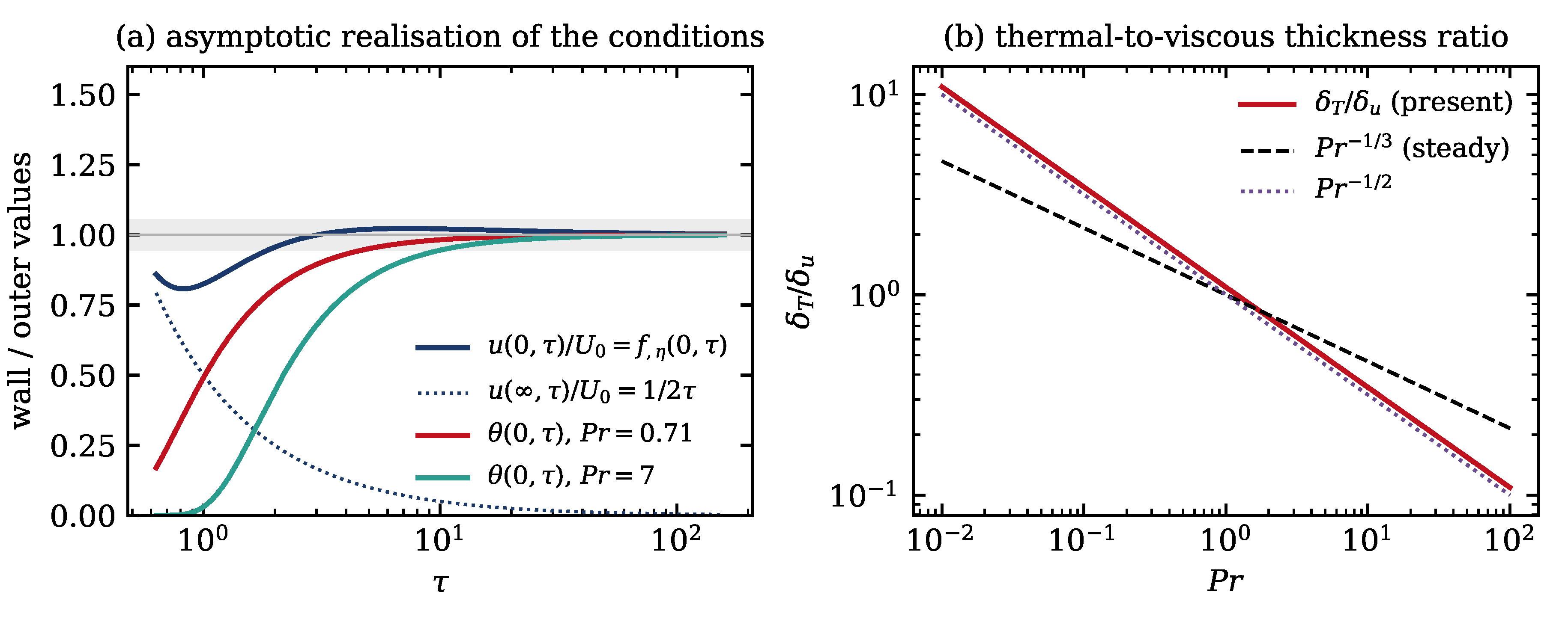
an exact power law at all . This is worth contrasting with the steady Prandtl–Blasius layer, in which the corresponding ratio crosses over from a behaviour at small to at large . No such crossover occurs here: both layers in the unsteady problem are diffusive rather than convective in structure, and the single exponent registers that difference (Figure 10b). The scaling in (53), in place of the of the Colburn analogy, has the same origin.
Because depends on x, y and t through , the isotherms in a fixed-t snapshot are not parallel to the plate. Figure 7(b) shows that the thermal footprint is confined to : information from the impulsively started heated plate has not yet reached stations further downstream, which is the correct physical behaviour and is encoded automatically in the similarity variable.
8. Comparison with the Quasi-Steady Practice
We can now quantify what is lost by using (2). Comparing (50) at with ,
the two agreeing only at , that is for air and for water. Since , at a station x the quasi-steady formula underestimates the wall heat flux for all times , and by a factor of two or more for . For the start-up of an air flow at 1 m s−1 over a m plate this is the whole of the first s, precisely the transient the unsteady energy equation was introduced to capture.
The profiles tell the same story. Figure 8(a) compares from (44) with the Pohlhausen profile at three stations at a fixed instant. The unsteady thermal layer has an x-independent thickness , so it is thicker than the quasi-steady prediction near the leading edge and thinner far downstream; the crossover is again at . A calculation that freezes the velocity field at Blasius therefore misrepresents both the magnitude and the streamwise trend of the transient.
9. Verification and Range of Validity
9.1. Numerical Verification
Table 2 lists the residuals of the momentum Equation (21) evaluated with (25)–(), and of the full unsteady energy Equation () evaluated with (41), in 25-digit arithmetic with derivatives obtained by Richardson-extrapolated central differences.
Because the cancellation of Section 3 is the step in the derivation most easily got wrong, it was also checked in a way that uses none of the transformation algebra. The fields , and were assembled in physical coordinates from (15) and (41), and the original Equations (4)–() evaluated by high-order finite differences in x, y and t. Continuity and momentum are satisfied by construction, so their residuals fix the noise floor of the differentiation. Table 3 reports the outcome, together with the residual obtained when the term is reinstated: the correct energy equation sits on the same noise floor as continuity and momentum, while the alternative is larger by twelve orders of magnitude.

Table 2.
Residuals of (21) and () at selected points, computed with 25 significant digits.
Table 2.
Residuals of (21) and () at selected points, computed with 25 significant digits.
| momentum residual | energy residual | ||||
|---|---|---|---|---|---|
| 0.5 | 1.0 | 0.71 | 0.0 | ||
| 1.0 | 2.0 | 0.71 | 1.0 | ||
| 0.4 | 1.5 | 7.0 | 0.0 | ||
| 2.0 | 3.0 | 7.0 | 2.0 | ||
| 0.2 | 0.9 | 0.1 | 1.0 | ||
| 3.0 | 5.0 | 1.0 | 0.5 |
Table 3.
Residuals of the original Equations (4)–() evaluated in physical variables with , , , step , 30-digit arithmetic. The last column is the energy residual obtained when the spurious term is retained.
Table 3.
Residuals of the original Equations (4)–() evaluated in physical variables with , , , step , 30-digit arithmetic. The last column is the energy residual obtained when the spurious term is retained.
| continuity | momentum | energy | energy, extra term | |
|---|---|---|---|---|
9.2. Sense in Which the Solution Is Exact
Throughout, exact is used in the sense standard for the Navier–Stokes literature [18,19,20]: the velocity and temperature fields satisfy the governing partial differential equations identically, for arbitrary viscosity and diffusivity, with no truncation, series expansion or numerical approximation. The boundary conditions, as in the parent velocity solution, are attained only asymptotically in . These statements are independent and both hold; the second is made quantitative next.
9.3. Attainment of the Boundary Conditions
Sun [16] imposes and at . At finite the compact form (33) makes the defect explicit and shows that a single mechanism is responsible for both. Since ,
a uniform drift superposed on the profile ; and since the same drift is present at the wall, where and ,
Equation (57) agrees with the exact wall value to four decimal places for (Figure 9a). Two consequences follow, and it is important to state them plainly.
First, the approach to no slip is not monotone. The term dominates at small and the term at large , so crosses unity at , reaches a maximum of at , and decays thereafter. Between and the fluid at the wall moves up to faster than the plate. The excess is small but it is a genuine violation of the no-slip condition, and any use of the solution in that range should acknowledge it.
Second, the two defects are of the same order. Both wall and outer conditions are satisfied to , so a single criterion governs both: lies within of unity for and within for (Figure 9b). The temperature inherits the same behaviour through ,
which approaches unity monotonically and from below, reaching accuracy at for air and for water (Table 4). Taken together, the quantitative statements of Section 7Section 8 should be read as carrying an uncertainty: a few per cent for , below for . In terms of the physical variables this is , so the solution describes the region near the leading edge, or equivalently the late-time behaviour at fixed x.
9.4. Further Limitations
The solution grows as and does not saturate at the Blasius thickness ; it is an exact member of a class of unsteady boundary layers rather than a description of the complete Rayleigh-to-Blasius transition. This is why h is independent of x, and why the ratio (55) decays without bound as grows.
The line is a degenerate characteristic of (): the coefficient vanishes as , so no Cauchy data are prescribed there. Consequently more than one exact solution satisfies the same asymptotic conditions; at both and do. Within the group-invariant class the solution (41) is unique, which is the natural similarity-theoretic statement. The practical spread is quantifiable: (48) gives exactly at , against from (53), and the difference may be taken as a measure of the residual indeterminacy.
Figure 10.
(a) Approach of the wall and outer values to their prescribed limits; the shaded band is . (b) The exact thickness ratio , Equation (54), compared with the steady estimate.
Figure 10.
(a) Approach of the wall and outer values to their prescribed limits; the shaded band is . (b) The exact thickness ratio , Equation (54), compared with the steady estimate.
10. Conclusions
The diffusion-time similarity transformation , transforms the unsteady energy equation into (19), with the same coefficients as the momentum equation. The terms in arising from and cancel identically. The coupled system closes only for , so the flat plate is the distinguished member of the family .
Sun’s exact velocity solution collapses to the three expressions (25)–() and is invariant under the one-parameter group generated by , with invariant and . In particular .
On group-invariant temperature fields the convective operator of the energy equation loses all dependence on the velocity field, and the unsteady thermal boundary layer reduces exactly to , the unsteady counterpart of the Pohlhausen equation. Its solutions are elementary: for an isothermal wall, and a recovery factor for an adiabatic wall. The engineering results are , , , , and h independent of x.
The prevailing practice of substituting the steady Blasius field into the unsteady energy equation misestimates the wall heat flux by ; the two agree only near , and over the whole early transient the discrepancy is of order unity. A consistent unsteady treatment of the velocity field is therefore not a refinement but a requirement.
Two extensions suggest themselves. A temperature field of the form would relax the large- restriction of Section 9 systematically, each order inheriting the same linear operator and requiring only a quadrature; the leading correction would in particular address the defect in the boundary conditions. More broadly, the mechanism identified in (37) is not special to this flow: whenever a boundary-layer solution is invariant under a one-parameter group, the convective operator restricted to invariant scalars becomes universal, and any passive scalar reduces to an ordinary differential equation with the velocity field entering only through a source term.
Author Contributions: Bo Hua Sun
: Conceptualization, Methodology, Formulations, Formal analysis, Funding acquisition, Investigation, Writing- Original draft preparation, Writing- Reviewing and Editing and all relevant works.
Data Availability Statement
The data supporting the findings of this study are available from the corresponding author upon reasonable request.
Acknowledgments
My investigations into the boundary layers started from my tenure as a professor at the Cape Peninsula University of Technology (CPUT), South Africa. I am profoundly grateful to CPUT for granting me complete academic autonomy to advance this research agenda. This vital institutional support laid the foundation for the principal conclusions presented in this manuscript. I also extend my deepest gratitude to former Vice-Chancellor (now Chancellor) Prof. Brian Figaji, and former Deputy Vice-Chancellors Prof. J. A. Tromp and Prof. Anthony Staak, for their generous support and endorsement. Further academic support was provided by Xi’an University of Architecture and Technology (XAUAT) and the Beijing Institute of Nanoenergy and Nanosystems (BINN), Chinese Academy of Sciences. I sincerely thank former XAUAT President Prof. Xiao-Jun Liu and current President Prof. Xiang-Mo Zhao, along with BINN Founding Director Prof. Zhong Lin Wang, for their unwavering encouragement and invaluable resource support throughout this study.
Conflicts of Interest
The authors declare that there are no competing financial interests.
Appendix A. Kummer Functions
The Kummer functions and are the two independent solutions of [1]. Only the second kind is needed here, being the solution that decays as , where . For ,
We use the contiguous relations
and, most importantly, the identity obtained by combining () (shifted ) with (),
which closes the successive derivatives ()–() on themselves and supplies the antiderivative used in Proposition 1. Two special values follow from (A1) with : , so the profile is correctly normalised, and .
Appendix B. Numerical Procedures
All symbolic checks were performed in 25–30 digit floating-point arithmetic. Derivatives with respect to , which are not available in closed form for f, were computed by Richardson-extrapolated central differences. Kummer functions were evaluated with standard confluent hypergeometric routines, cross-checked between two independent implementations to over .
The quadratures in (42) and (43) contain the factor , which overflows for large . They are therefore evaluated in the scaled forms
both bounded for , where . The upper limit served as numerical infinity, the integrands decaying as .
The steady reference solutions were obtained by shooting, giving and at and at , in agreement with the classical tabulations [10].
References
- Abramowitz, M. & Stegun, I. A. 1972 Handbook of Mathematical Functions, ch. 13. Dover.
- Blasius, H. 1908 Grenzschichten in Flüssigkeiten mit kleiner Reibung. Z. Math. Phys. 56, 1–37.
- Dennis, S. C. R. 1972 Motion of a viscous fluid past an impulsively started semi-infinite flat plate. IMA J. Appl. Maths 10, 105–117.
- Hall, M. G. 1969 The boundary layer over an impulsively started flat plate. Proc. R. Soc. Lond. A 310, 401–414.
- Hassan, H. A. 1960 On unsteady laminar boundary layers. J. Fluid Mech. 9, 300–304.
- Ma, P. K. H. & Hui, W. H. 1990 Similarity solutions of the two-dimensional unsteady boundary-layer equations. J. Fluid Mech. 216, 537–559.
- Pohlhausen, K. 1921 Zur näherungsweisen Integration der Differentialgleichung der laminaren Grenzschicht. Z. Angew. Math. Mech. 1, 252–268.
- Rayleigh, Lord 1911 On the motion of solid bodies through viscous liquids. Phil. Mag. 21, 697–711.
- Riley, N. 1975 Unsteady laminar boundary layers. SIAM Rev. 17, 274–297.
- Schlichting, H. & Gersten, K. 2017 Boundary Layer Theory, 9th edn. Springer.
- Stewartson, K. 1951 On the impulsive motion of a flat plate in a viscous fluid. Q. J. Mech. Appl. Maths 4, 182–198.
- Stewartson, K. 1960 The theory of unsteady laminar boundary layers. Adv. Appl. Mech. 6, 1–37.
- Stewartson, K. 1973 On the impulsive motion of a flat plate in a viscous fluid, II. Q. J. Mech. Appl. Maths 26, 143–152.
- Stokes, G. G. 1851 On the effect of the internal friction of fluids on the motion of pendulums. Trans. Camb. Phil. Soc. 9, 8–106.
- Stuart, J. T. 1963 Unsteady Boundary Layers, pp. 349–408. Clarendon.
- Sun, B. H. 2024 Similarity solutions of a class of unsteady laminar boundary layer. Phys. Fluids 36, 083616.
- Takuda, K. 1968 On the impulsive motion of a flat plate in a viscous fluid. J. Fluid Mech. 33, 657–675.
- Wang, C. Y. 1989 Exact solutions of the unsteady Navier–Stokes equations. Appl. Mech. Rev. 42, S269–S282.
- Wang, C. Y. 1991 Exact solutions of the steady-state Navier–Stokes equations. Annu. Rev. Fluid Mech. 23, 159–177.
- Wang, C. Y. 2024 Essential Analytic Laminar Flow. Springer Nature.
- Ovsiannikov, L. V. 1962 Group Analysis of Differential Equations (in Russian). Nauka, Moscow, 1962. (English translation: Ames, W.F. (Ed.), 1982. Academic Press, New York.).
- Sun, B. H. 2016 Dimensional Analysis and Lie Group(In Chinese). China Higher Education Press.
Figure 1.
A semi-infinite flat plate held at temperature is set in relative motion with velocity at in a fluid at . For (that is, ) leading-edge information has arrived and the layer is quasi-steady; for () the layer is still purely unsteady and grows as , independently of x.
Figure 1.
A semi-infinite flat plate held at temperature is set in relative motion with velocity at in a fluid at . For (that is, ) leading-edge information has arrived and the layer is quasi-steady; for () the layer is still purely unsteady and grows as , independently of x.
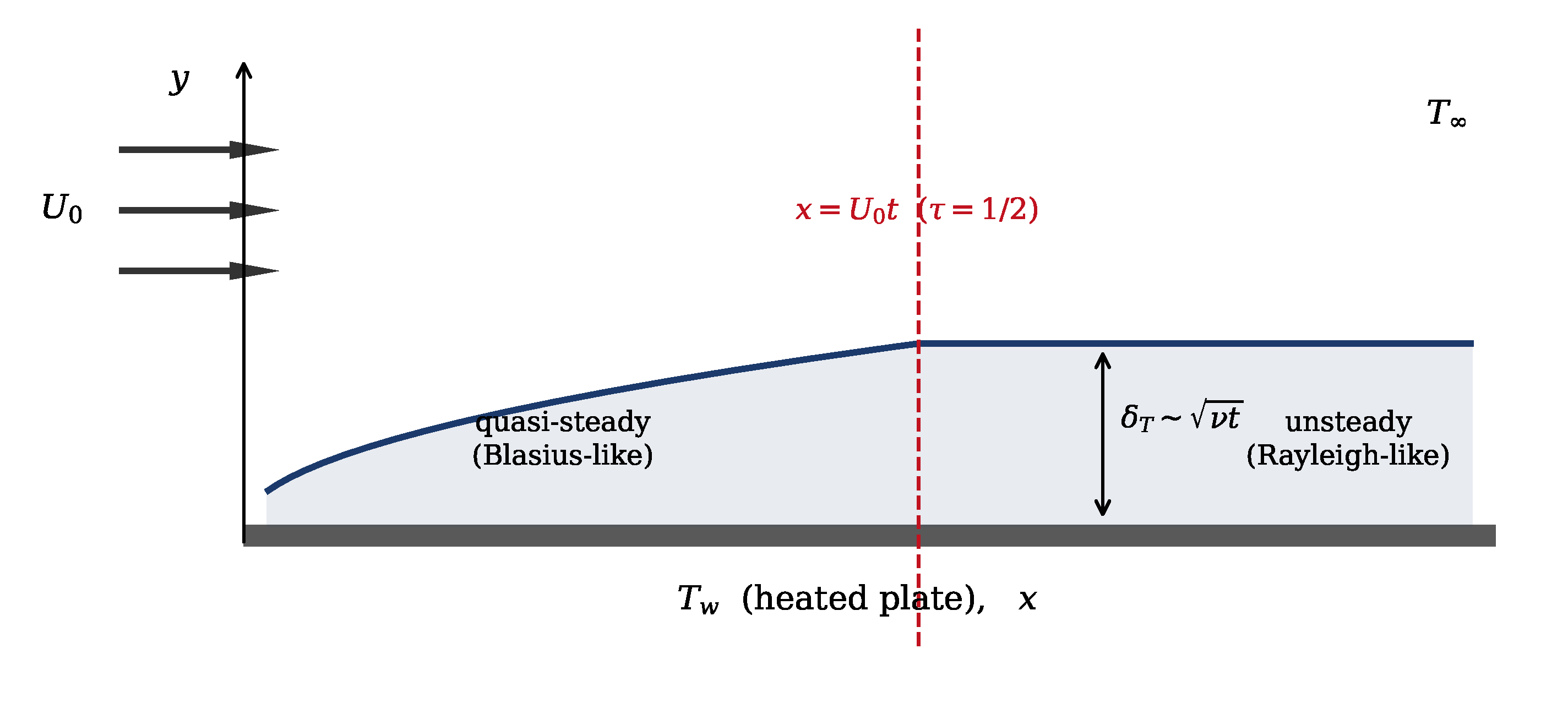
Figure 2.
(a) The universal profile of (33), its derivative and the dissipation kernel . (b) against at fixed ; dotted lines mark the residual outer drift , which vanishes as .
Figure 2.
(a) The universal profile of (33), its derivative and the dissipation kernel . (b) against at fixed ; dotted lines mark the residual outer drift , which vanishes as .
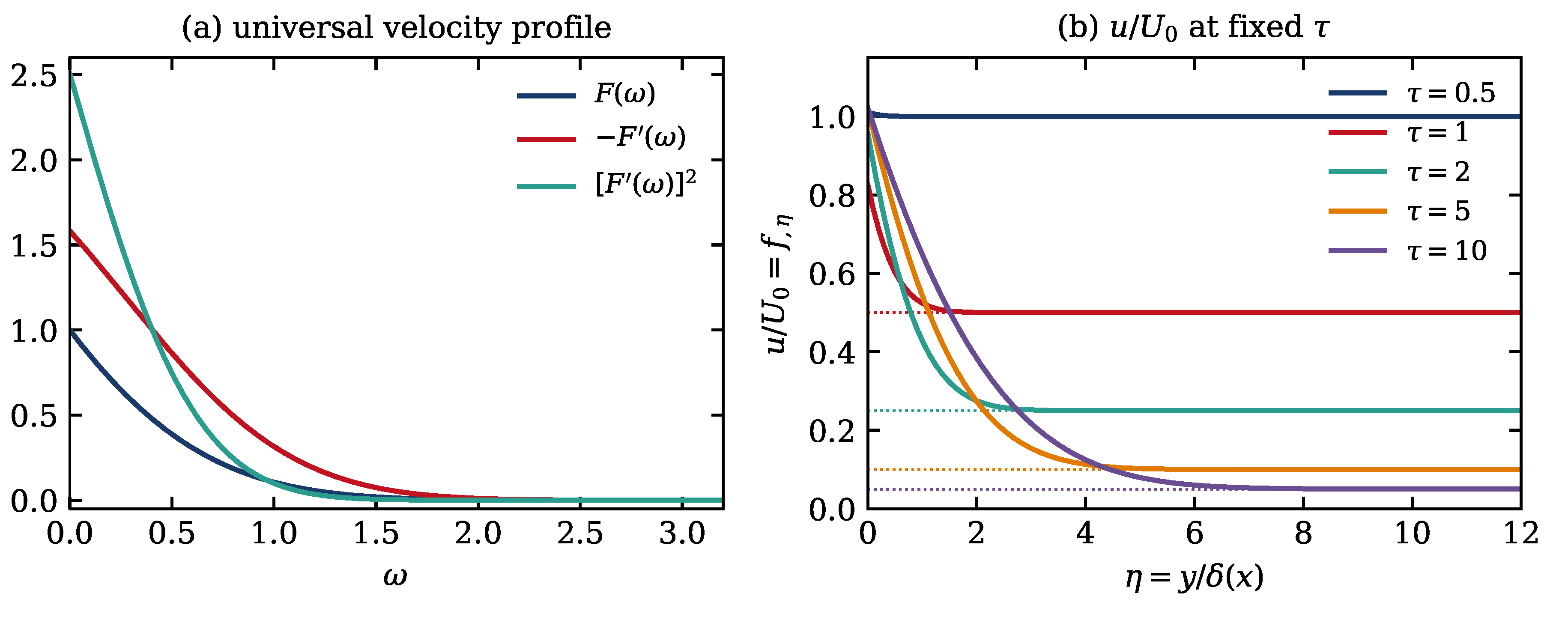
Figure 3.
(a) Temperature profiles (44) for ; the dashed curve is the velocity profile . (b) Wall gradient and recovery factor , with the steady value for reference.
Figure 3.
(a) Temperature profiles (44) for ; the dashed curve is the velocity profile . (b) Wall gradient and recovery factor , with the steady value for reference.
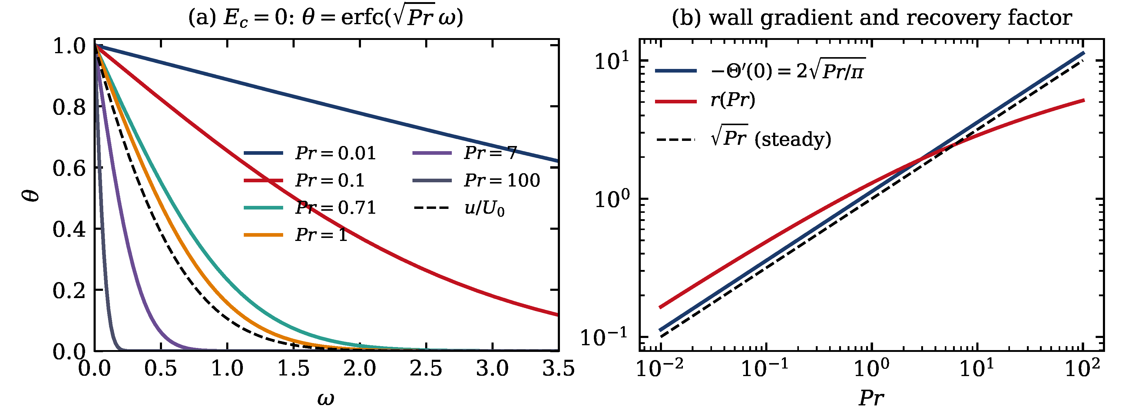
Figure 4.
Effect of viscous dissipation on the isothermal-wall profiles. At the wall gradient vanishes; beyond it the wall is heated by the fluid and overshoots unity.
Figure 4.
Effect of viscous dissipation on the isothermal-wall profiles. At the wall gradient vanishes; beyond it the wall is heated by the fluid and overshoots unity.
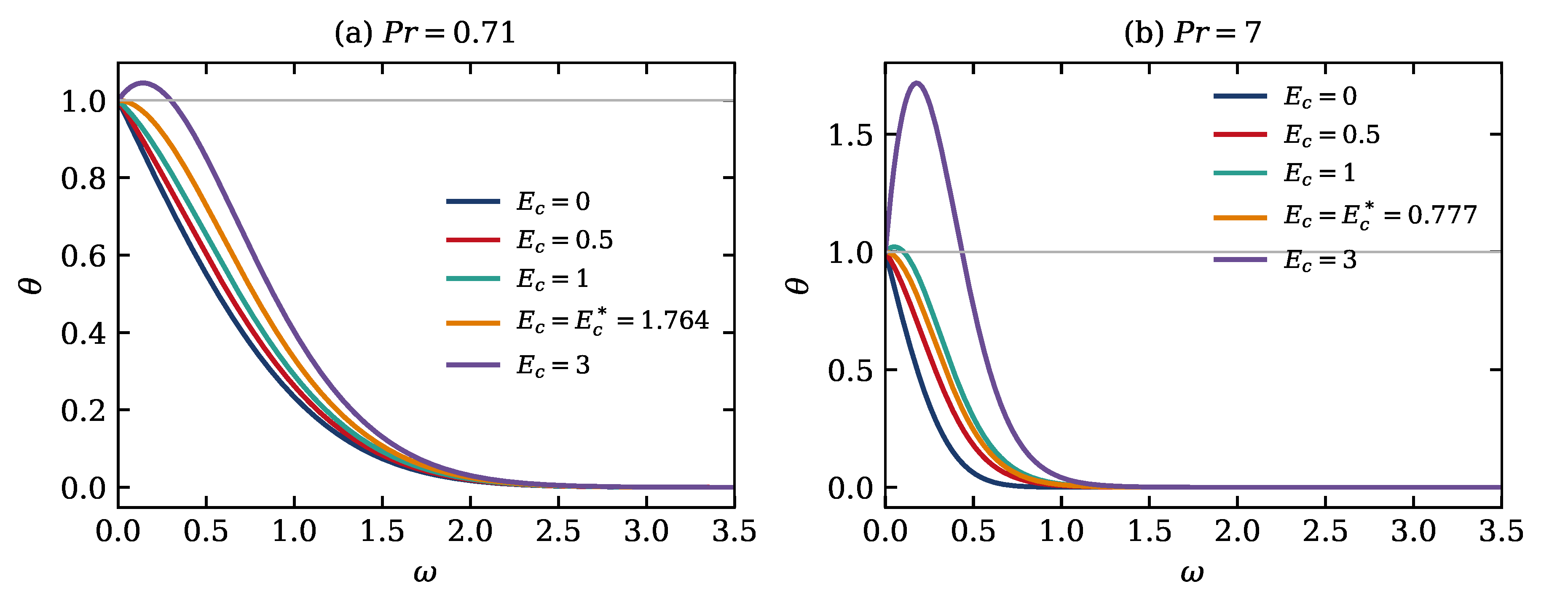
Figure 5.
(a) Adiabatic-wall temperature distributions normalised by . (b) Recovery factor (45) with the limits (46) and (47), and the steady value .
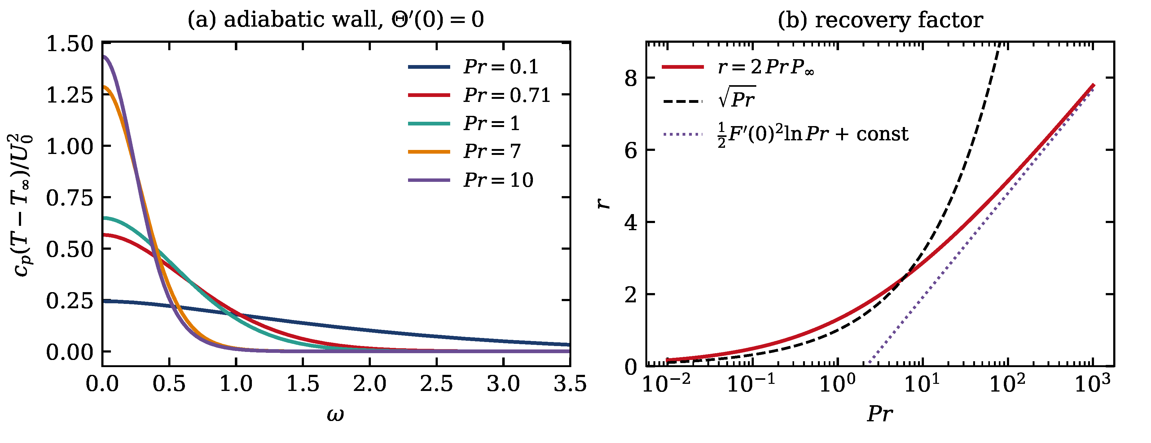
Figure 6.
(a) Reduced Nusselt number against for several Eckert numbers; it changes sign at . (b) Critical Eckert number (52).
Figure 6.
(a) Reduced Nusselt number against for several Eckert numbers; it changes sign at . (b) Critical Eckert number (52).
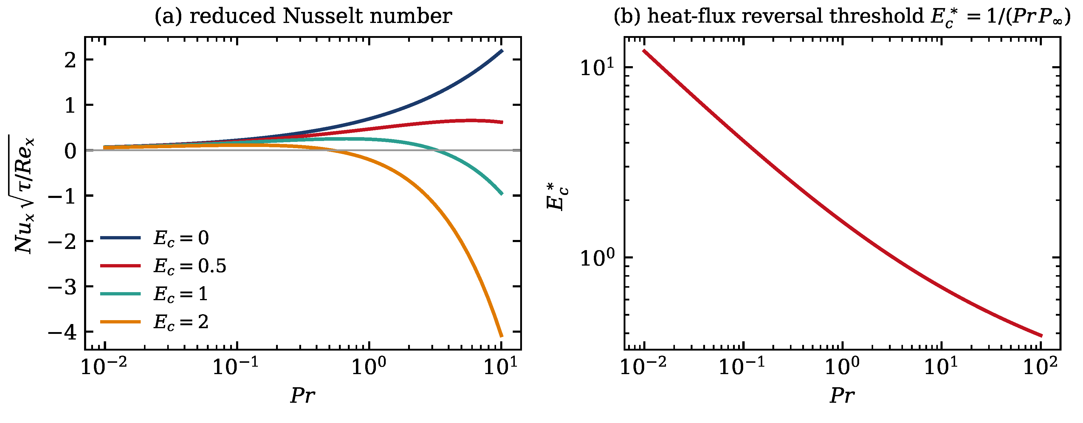
Figure 7.
(a) for air at . (b) The same field in physical coordinates at s for m s−1, m2 s−1. The heated region does not extend beyond .
Figure 7.
(a) for air at . (b) The same field in physical coordinates at s for m s−1, m2 s−1. The heated region does not extend beyond .
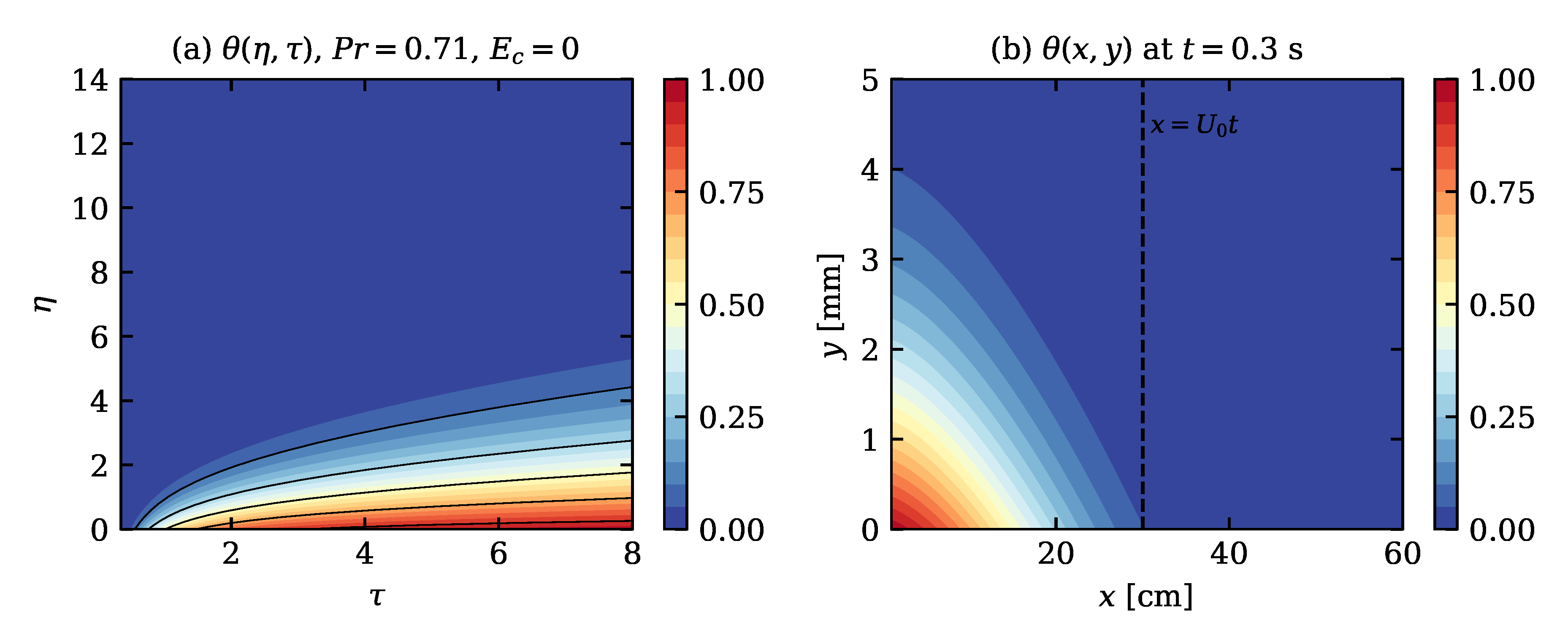
Figure 8.
(a) Temperature profiles at s and three stations (solid, present theory; dashed, Blasius–Pohlhausen at the same x) for air, m s−1. (b) Ratio (55) of exact to quasi-steady Nusselt numbers.
Figure 8.
(a) Temperature profiles at s and three stations (solid, present theory; dashed, Blasius–Pohlhausen at the same x) for air, m s−1. (b) Ratio (55) of exact to quasi-steady Nusselt numbers.
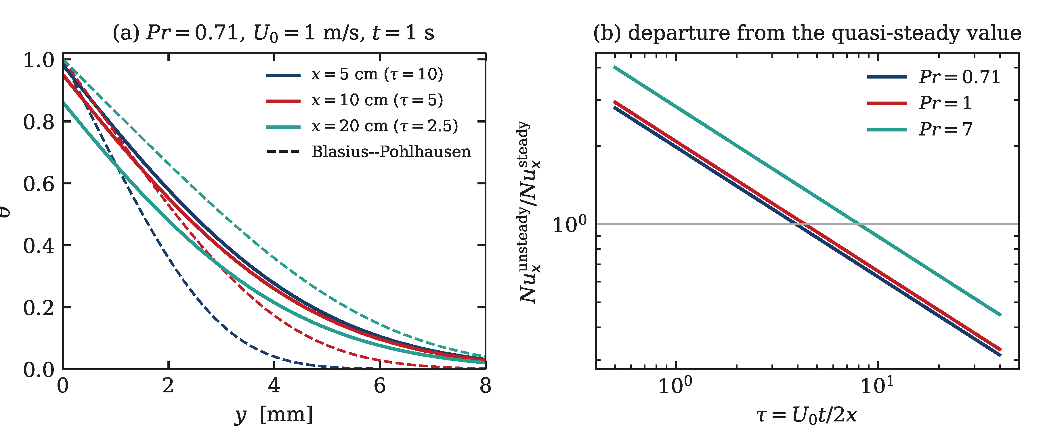
Figure 9.
(a) Wall velocity against , with the asymptotic form (57); the shaded band is . The no-slip condition is under-satisfied for and over-satisfied beyond, with a maximum excess of at . (b) Wall and outer defects compared; both decay as .
Figure 9.
(a) Wall velocity against , with the asymptotic form (57); the shaded band is . The no-slip condition is under-satisfied for and over-satisfied beyond, with a maximum excess of at . (b) Wall and outer defects compared; both decay as .
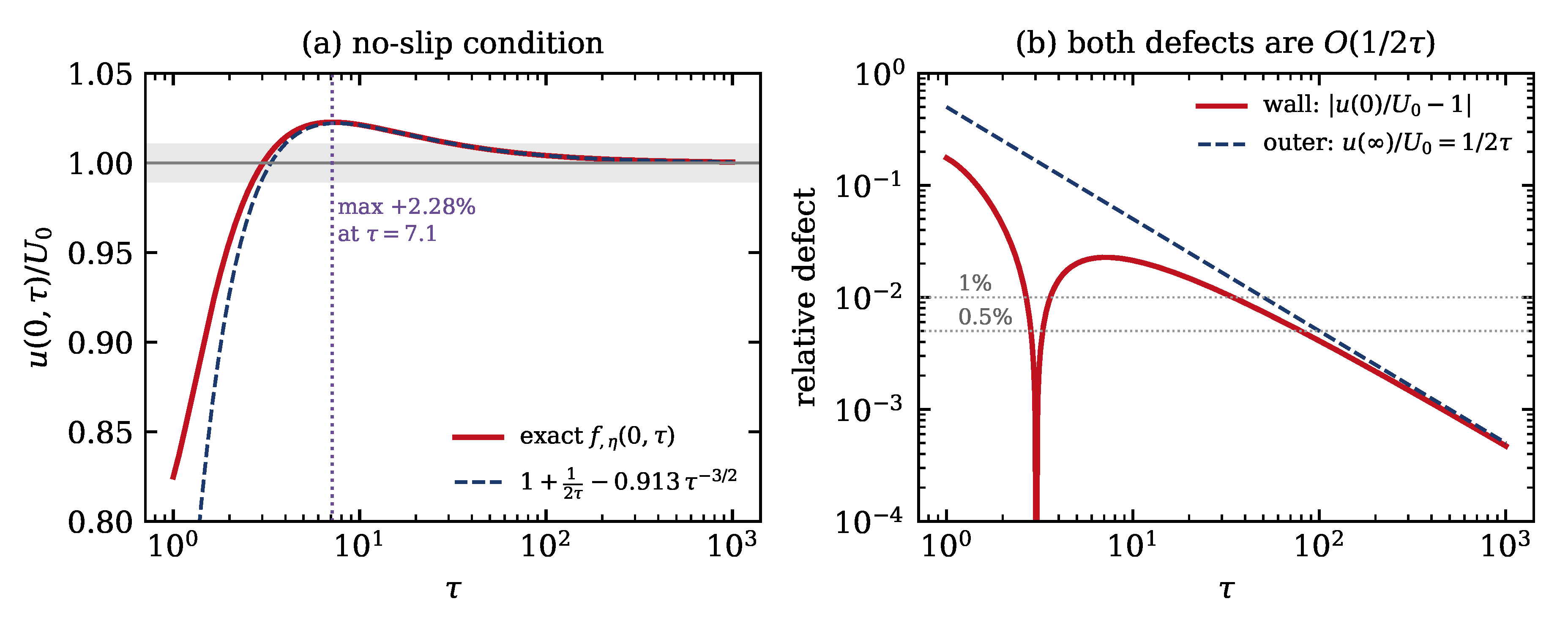
Table 1.
Similarity results as functions of the Prandtl number. Here is the wall gradient at , is defined in (43), r in (45), in (52) and in (54).
| r | |||||
|---|---|---|---|---|---|
| 0.01 | 0.11284 | 8.24313 | 0.16486 | 12.13132 | 10.91020 |
| 0.1 | 0.35682 | 2.43925 | 0.48785 | 4.09962 | 3.45011 |
| 0.5 | 0.79788 | 0.98276 | 0.98276 | 2.03509 | 1.54293 |
| 0.71 | 0.95079 | 0.79838 | 1.13369 | 1.76415 | 1.29480 |
| 1 | 1.12838 | 0.64912 | 1.29824 | 1.54055 | 1.09102 |
| 2 | 1.59577 | 0.42140 | 1.68561 | 1.18652 | 0.77147 |
| 5 | 2.52313 | 0.23119 | 2.31191 | 0.86509 | 0.48792 |
| 7 | 2.98541 | 0.18384 | 2.57381 | 0.77706 | 0.41237 |
| 10 | 3.56825 | 0.14346 | 2.86913 | 0.69708 | 0.34501 |
| 50 | 7.97885 | 0.04398 | 4.39781 | 0.45477 | 0.15429 |
| 100 | 11.28379 | 0.02567 | 5.13480 | 0.38950 | 0.10910 |
Table 4.
Attainment of the boundary conditions with increasing . The wall velocity attains a maximum excess of at .
Table 4.
Attainment of the boundary conditions with increasing . The wall velocity attains a maximum excess of at .
| 1 | 0.82480 | 0.50000 | 0.57735 | 0.49146 | 0.03075 |
| 2 | 0.95604 | 0.25000 | 0.20412 | 0.80782 | 0.44501 |
| 3 | 0.99932 | 0.16667 | 0.11111 | 0.89466 | 0.67760 |
| 5 | 1.02010 | 0.10000 | 0.05164 | 0.95093 | 0.84679 |
| 7.13 | 1.02276 | 0.07013 | 0.03031 | 0.97117 | 0.90862 |
| 10 | 1.02134 | 0.05000 | 0.01826 | 0.98264 | 0.94554 |
| 20 | 1.01481 | 0.02500 | 0.00645 | 0.99386 | 0.98073 |
| 50 | 1.00742 | 0.01000 | 0.00163 | 0.99845 | 0.99512 |
| 100 | 1.00409 | 0.00500 | 0.00058 | 0.99945 | 0.99828 |
Disclaimer/Publisher’s Note: The statements, opinions and data contained in all publications are solely those of the individual author(s) and contributor(s) and not of MDPI and/or the editor(s). MDPI and/or the editor(s) disclaim responsibility for any injury to people or property resulting from any ideas, methods, instructions or products referred to in the content. |
© 2026 by the authors. Licensee MDPI, Basel, Switzerland. This article is an open access article distributed under the terms and conditions of the Creative Commons Attribution (CC BY) license (http://creativecommons.org/licenses/by/4.0/).
Copyright: This open access article is published under a Creative Commons CC BY 4.0 license, which permit the free download, distribution, and reuse, provided that the author and preprint are cited in any reuse.