

Submitted:
19 August 2026
Posted:
20 August 2026
You are already at the latest version
Abstract
Accurate and computationally efficient numerical modelling of shallow-water flows is essential for flood prediction and hydrodynamic risk assessment. This study develops an implicit finite-difference scheme for the numerical solution of the two-dimensional shallow water equations. First, the main numerical approaches used for shallow-water modelling, including finite-difference, finite-volume, finite-element, and discontinuous Galerkin methods, are analysed in terms of accuracy, stability, treatment of discontinuities, and computational requirements. Based on this analysis, an implicit finite-difference formulation is developed that uses central approximations for spatial derivatives and averages flow variables at cell boundaries. The nonlinear terms are treated using Newton linearization, resulting in an iterative scheme that allows larger time steps than explicit formulations constrained by the Courant-Friedrichs-Lewy condition. The proposed method is implemented in MATLAB as a computational module for two-dimensional hydrodynamic simulations. Its performance is demonstrated on a test problem that describes the propagation of an initially localised disturbance in a rectangular computational domain with rigid boundaries. The numerical results demonstrate stable wave propagation, conservation of the modelled flow dynamics, and physically consistent boundary reflections. The developed approach provides a computational basis for further integration of shallow-water hydrodynamic models with spatial data and geographic information systems for flood forecasting and risk assessment.
Keywords:
computational hydrodynamics
; implicit finite-difference scheme
; shallow water equations
; Newton linearization
; geographic information system
1. Introduction
The current stage of development in Earth sciences and engineering hydrology is characterised by a profound transformation in approaches to studying water systems [1,2,3]. Simplified, static assessment methods are being replaced by complex, dynamic models that can reproduce the evolution of natural and anthropogenic processes across space and time. In this context, the shallow water equation system occupies a unique position as a fundamental theoretical basis, ensuring a balance between the physical completeness of the description of the phenomenon and computational feasibility [1,4,5,6]. However, a true revolution in the capabilities of analysis and forecasting is taking place at the intersection of this mathematical theory with geoinformation system technologies. The integration of shallow water equations and geoinformation systems forms a new research paradigm, in which abstract hydrodynamic calculations acquire spatial specificity, transforming them into tools for management decision-making, risk assessment, and engineering design.
The mathematical model of the system in conservative form for modelling the processes investigated in this work takes the form [2,3]:
where H(x,y,t) is the total water depth; u(x,y,t) is the velocity along x; v(x,y,t) is the velocity along y; g is the acceleration due to gravity.
The shallow water equations represent a class of hyperbolic partial differential equations that describe the motion of a fluid with a free surface in a gravitational field. Their derivation from the full three-dimensional Navier–Stokes equations via a depth-averaging procedure is based on the key physical assumption of a hydrostatic pressure distribution, which holds for the vast majority of geophysical flows in which the horizontal scales significantly exceed the vertical ones [3,7]. This simplification is not a shortcoming, but rather a methodological tool that allows secondary vertical accelerations to be filtered out, focusing on the dominant horizontal transport of mass and momentum.
The relevance of these equations in modern research stems from their ability to reproduce a wide spectrum of wave motions critical to understanding the dynamics of the oceans, seas and planetary atmospheres. In particular, they accurately describe high-frequency inertial-gravitational waves (Poincare waves), which are responsible for the rapid redistribution of energy within a basin, and low-frequency Rossby waves, whose dynamics determine synoptic variability and large-scale circulation [7,8,9]. It is precisely this ability to model multi-scale processes that makes shallow-water equations and their modifications indispensable tools in oceanography, limnology, and river hydraulics for the study of inundations, floods, and tsunami surges onto coasts (Figure 1).
Studies aimed at accounting for the medium’s variable density and compressibility are of particular importance [7,10,11]. The development of ‘compressible shallow water equations’ models paves the way for modelling fundamentally new classes of phenomena. This concerns not only dust storms on Mars or two-phase flows under terrestrial conditions (for example, the transport of sediments or snow-dust masses), but also fundamental processes in astrophysical discs, where gravitational interaction and compressibility play a decisive role.
Another revolutionary direction is the synergy of classical hydrodynamic models with machine learning methods [12,13,14]. The current trend lies in the creation of so-called “universal” or “data-driven hydrodynamic models” [13,15]. Applying differential programming to shallow-water equations allows not only for solving equations with pre-defined parameters, but also for “training” the model based on available observations. This makes it possible, for example, to identify the spatial distribution of the Manning roughness coefficient with unprecedented accuracy, adapting the model to the local characteristics of the river channel and floodplain, which is critical for reliable flood zone forecasting [15,16,17].
The greatest practical potential of shallow water equations is realised precisely through their close integration with geographic information systems [18]. Such a system ceases to be merely a tool for visualising final results. It becomes an integral component of the entire modelling cycle – from the preparation of input data to the interpretation of the results obtained.
The foundation of any hydrodynamic calculation is a digital elevation model, which serves as the spatial basis for constructing the computational grid [16,19,20]. It is through the use of geographic information systems that hydrologically correct processing of the digital elevation model is carried out – removal of artefacts, “filling” of closed depressions, and calculation of surface runoff directions. Next, using geoprocessing tools, raster and vector layers containing information on spatially distributed parameters—such as substrate types, vegetation cover and soils—are overlaid onto the study area. Each of these types is assigned numerical values for hydraulic resistance (roughness coefficients), which allows the model to respond appropriately to landscape heterogeneity (Figure 2) [20,21].
The model verification process also takes on a new dimension thanks to modern geoinformation systems. Modelling results (velocity fields, depths, free-surface levels) are imported back into the GIS environment for comparison with Earth remote sensing data, ground-based hydrological stations, or historical flood maps [10,16]. Such spatial analysis allows not only a visual assessment of the model’s adequacy, but also the calculation of quantitative accuracy metrics.
It should be noted that the implementation of the shallow water equation system using explicit schemes, despite their high speed, has significant limitations on the time step due to the Courant–Friedrichs–Lewy condition, which is given by [1]:
The value of the parameter CFL≈0.5 for 2D explicit schemes; CFL ≤ 1 for explicit 1D schemes and for Lax-Friedrichs-type schemes – typically 0.3–0.5.
The synthesis of hydrodynamic models based on shallow-water equations and the analytical capabilities of geographic information systems creates a powerful toolkit for solving a wide range of applied problems in national security, the economy, and ecology [22,23,24]. In the field of natural disaster risk management, a key task is the creation of flood hazard and risk maps. The application of these equations enables the modelling of the dynamics of flood waves, the passage of catastrophic floods with varying return periods, and storm surges. Integrating these scenarios into geographic information systems enables quantification of the population at risk, identification of critical infrastructure at risk (bridges, hospitals, chemical plants), and calculation of expected economic losses. This provides a scientifically sound basis for spatial planning, insurance and the development of evacuation plans.
In environmental terms, this combination of technologies enables the prediction of pollutant migration in water bodies. By modelling currents using such equations and superimposing contaminant movement trajectories onto them, it is possible to predict with high accuracy the zones of pollutant sedimentation, including heavy metals, petroleum products, and radionuclides [8,14]. This approach is indispensable for assessing the impact of accidental discharges, designing water protection zones, and justifying remediation measures for disturbed areas.
2. Analysis of Shallow Water Equation Modelling Methods
The choice of method depends on the specific physics of the process and engineering requirements. Recent comparative studies allow the following generalisations.
For smooth flows, high-order methods and compact finite-difference methods yield the best results. For flows with discontinuities (e.g., hydraulic jumps), the finite volume method (particularly the counter-flow scheme) is the natural choice due to its conservativeness and ability to localise the wave front accurately. For example, the abstract of one of the studies notes that the developed high-precision scheme significantly outperforms other methods in accuracy, reducing error by several orders of magnitude. A comparison of the above methods has shown that both are reliable for quasi-steady states that account for friction, but require different approaches to approximating the source terms. A critical requirement for modern schemes is the property of balance. The finite element and finite volume methods achieve this through a special approximation of the source term, such as the seabed topography. For the finite volume method, this means that the scheme must accurately solve the given problem in the corresponding mathematical formulation [1].
Traditional finite-difference methods on structured grids are the fastest. Finite-volume methods offer a good balance between speed and accuracy. The finite-element method and the Galerkin method are more computationally expensive, but their advantage in accuracy on complex grids may offset this drawback. A study of methods for the local inertia equation showed that implicit methods have the highest stability and the smallest error when modelling the water-land boundary, whereas the exponential method can produce oscillations. A summary comparison of the flood modelling methods considered that use shallow-water equations is given in Table 1.
Traditional finite-difference schemes on regular grids. These are historically the first and most extensively studied approaches. They are based on approximating derivatives with finite-difference analogues on structured grids. This category includes such well-known schemes as the Lax–Friedrichs, Lax–Wendroff, and McCormack schemes, among others, which are described in detail in the classical literature. The high computational speed of these methods is their main advantage. Thanks to the simplicity of the data structures and the regularity of the computations, they lend themselves excellently to vectorisation and parallelisation, making them the fastest of all methods. The basic schemes are relatively easy to programme, making them attractive for rapid prototyping. As a recent comparative study has shown, one of the traditional finite-difference schemes demonstrated the best accuracy in modelling large-scale ocean currents and storm surges on the shelf.
It is also worth noting the shortcomings of such schemes. One such shortcoming is the poor approximation of complex geometries. The use of rectangular grids yields a ‘stepped’ approximation of the coastline, leading to significant errors, particularly in complex coastal areas. Classic high-order schemes (e.g., Lax–Wendroff) generate undesirable oscillations (discontinuities) near hydraulic jumps. First-order schemes (Lax–Friedrichs) are monotonic but have high scheme viscosity, which ‘smears’ sharp wave profiles. Such schemes require special procedures to ensure the exact conservation of the state of rest over an uneven seabed. To overcome the geometry problem, modifications have been developed to better represent curved boundaries on a rectangular grid. For example, the technique of introducing diagonal segments in addition to vertical and horizontal ones to denote the ‘water-land’ boundary. In this case, significantly higher accuracy is achieved in coastal zones than with the traditional stepwise approach, without the need for excessive grid refinement. This approach yields more accurate results without a significant increase in the number of grid nodes, thereby reducing computational time. Of course, it should be noted that programme implementation is more complex – it requires modifying classical algorithms and implementing more complex programme logic. However, this approach still lags behind unstructured grids in terms of flexibility, which are used in the finite element and finite difference methods.
Mesh-free generalised finite difference methods represent a modern direction in the development of classical difference methods, designed to overcome the limitations of structured meshes. These modifications enable the construction of difference approximations with irregularly spaced nodes, significantly increasing the method’s flexibility. It is worth noting the flexibility of such methods, as they can handle complex geometries without requiring a grid, which is their main advantage over classical finite-difference methods. In such methods, high accuracy can be achieved on smooth solutions. There are spatio-temporal versions of generalised difference methods that demonstrate high efficiency and stability, for example, for the Korteweg–de Vries and regularised long-wave equations, which are models of dispersive waves in shallow water. Of course, the selection of neighbouring nodes for approximation and the construction of system matrices for each point are considerably more computationally expensive than simple indices in a structured grid. The method is considerably more complex to programme than the classical finite-difference method. It is not as well-established a standard for shallow-water equations as the finite-volume method.
Finite difference method for dispersive shallow-water equations. A distinct class is formed by difference schemes developed to solve non-classical, dispersive shallow-water models (of the Businescu type) that describe wave propagation while accounting for frequency dispersion. This method and its modifications allow the modelling of phenomena that are inaccessible to classical, non-dispersive shallow-water equations, such as the transformation of a tsunami in deep water. Research shows that the stability conditions for finite-difference schemes approximating dispersive equations are weaker than for schemes approximating classical shallow-water equations. However, in this case, the analysis of the dispersive and dissipative properties of such schemes is considerably more complex. It should also be noted that, for two-dimensional cases, there is the problem of the scheme’s phase error depending on the direction of wave propagation, which requires the development of special, rotation-invariant schemes.
Simplified finite-difference schemes for approximating the kinematic wave. For very simple configurations, the simplified form of the Saint-Venant equations – the kinematic wave equations – is used instead of the full equations. These are the simplest of all methods, very fast and stable under certain conditions. These methods do not work in the presence of a backwater, in the presence of changes in flow direction, or on complex terrain with steep gradients. They are unsuitable for most engineering problems on rivers. A comparative table of the main known difference methods used in oceanography is given below (Table 2).
3. Proposed Method
To construct an implicit difference scheme for (1), we shall first construct an explicit difference scheme, the principle of which will also be used for the implicit difference scheme. Let us assume we have a structured rectangular grid with nodes of the type , where
All subsequent calculations will form a system of equations in discrete form for the internal nodes of the computational domain, i.e., for In this case, the discrete analogue of the first equation of the shallow water equation system for any internal node can be expressed as follows:
It is clear that in (2) nodes of type
have non-integer indices. In this case, it is possible and even recommended to use an approximate representation via average values, i.e., via the expressions:
Let us substitute expressions (3) into (2) for the first equation of the shallow water equation system (1). As a result, we obtain:
The final finite difference scheme for the discrete version of the first equation of the shallow water equation system of the form (1):
In expression (5), the central element (node (i, j, k+1)) is expressed in terms of nodes of the form (*, *, k).
Similarly, the discrete analogue of the second equation of the shallow water equation system, presented in conservative form (1), is formulated. We write it as follows:
In expression (6), the expressions for the central difference derivatives are taken into account:
For expression (7), we finally obtain the expression for :
In (8), just as in (4), the following was taken into account:
Thus, we finally have:
The final step is to formulate a discrete analysis for the third equation of the shallow water equation system (1). We shall use central difference schemes to approximate the derivatives with respect to the spatial coordinates and . In this case, we obtain:
Multiplying both sides of (10) by , and expanding the terms with indices of the form (*, *, k+1), we obtain:
Now we obtain the final expression for . It takes the following form:
Finally, we have three difference equations for the explicit difference scheme:
We now proceed to derive an implicit difference scheme for (1). It will be based on the fundamental idea of the Crank-Nicolson scheme, which has proven to be quite effective in modelling complex systems and processes described by hyperbolic and parabolic equations with respect to time.
For the first equation, we obtain the following expression based on the Crank-Nicholson scheme:
Therefore, the discrete form of the first equation in (1) is
Taking into account expressions of the form (3), the first equation (1) can be rewritten as:
In expression (13), the terms with superscripts (k+1) have been deliberately left without using a formula of the form (3). This was done deliberately, as it is simpler from a mathematical and computational point of view to linearise these terms first and then approximate the elements with non-integer indices, rather than the reverse – approximating the elements using formulas of the form (3) and then linearising them. In the latter case, there are two main drawbacks: the accuracy of the approximation will be lower, and the number of terms requiring linearisation after expanding the brackets will be significantly greater.
Similarly, a discrete analogue of the second equation can be constructed for a system of equations of type (1). It takes the form:
If we substitute the formula of type (3) into the latter expression, we obtain:
The same principle is used to discretise the third equation of system (1). We have:
The final difference equation for the third shallow water equation after the transformations will be:
In expression (15), just as in expression (13), the terms with superscripts (k+1) have been deliberately left without using a formula of type (3).
The next step is to linearise the non-linear terms in the circuit. We have the following non-linear functions of the form: First, we shall implement the non-linear function with one unknown Based on Newton’s linearisation, we obtain:
Therefore:
For the node at time step k+1, we have:
For the node at time step k+1, we have:
For the node at time step k+1, we have:
For the node at time step k+1, we have:
Next, we perform linearisation using Newton’s method for the non-linear function . We obtain:
Therefore:
Using (17) for the node at time step k+1, we have:
Using (17) for the node at time step k+1, we have:
Using (17) for the node at time step k+1, we have:
Using (17) for the node at time step k+1, we have:
Newton’s linearisation of the function takes the following form:
Then using (18) for the node at time step k+1:
for the node at time step k+1:
for the node at time step k+1:
for the node at time step k+1:
Now let us perform linearisation using Newton’s method for the non-linear function . We obtain:
Therefore:
Then using (19) for the node at time step k+1:
for the node at time step k+1:
for the node at time step k+1:
for the node at time step k+1:
Let us perform linearisation using Newton’s method for the non-linear function . We obtain:
Then using (20) for the node at time step k+1:
for the node at time step k+1:
for the node at time step k+1:
for the node at time step k+1:
Finally, we perform linearisation using Newton’s method for the non-linear function . We obtain:
Therefore:
Then using (21) for the node at time step k+1:
for the node at time step k+1:
for the node at time step k+1:
for the node at time step k+1:
Finally, we obtain an iterative implicit scheme for (1), consisting of discrete analogues of equations (13)–(15) and an iterative linearisation procedure (16)–(21).
4. Developed Simulation Software
The developed software module is intended for numerical modelling of two-dimensional hydrodynamic processes in shallow water bodies, based on the nonlinear shallow-water equations. The module is implemented in the MATLAB environment as a single executable file, which provides a full cycle of calculations - from initialization of model parameters to saving and visualization of results. It is based on a fully implicit finite-difference scheme on a uniform rectangular grid, which guarantees unconditional stability of the calculations and allows the use of significant time-integration steps, regardless of Courant restrictions. Spatial discretization is performed with second-order accuracy, and integration over time is performed using the implicit Euler scheme of the first order.
To overcome the nonlinearity of the original system at each time step, Newton’s iterative method is used, which provides quadratic convergence in the vicinity of the solution. In the process of linearization, the partial derivatives of all nonlinear flow terms are analytically calculated, thereby avoiding errors from numerical differentiation. At each iteration, a system of linear algebraic equations with a sparse strip matrix is formed, which is diagonally dominant due to the locality of finite-difference patterns.м The solution of this system is performed by the direct method using the built-in MATLAB tools for working with sparse matrices, which ensures high reliability and accuracy of calculations. The maximum absolute error criterion across all grid nodes controls the convergence of the iterations.
Flexible settings characterise the software module: the user can specify the dimensions of the computational domain, grid spacing, time integration step, relaxation parameters, and initial conditions as a localised perturbation of the free surface. Initial velocities are taken equal to zero, which corresponds to a state of rest until the moment of perturbation. No-flow conditions are applied at the domain boundaries to simulate the reflection of waves from the impermeable walls of a closed reservoir. The modelling results are presented as two-dimensional and three-dimensional colour maps of the free-surface height distribution, as well as an automatically generated animation that allows you to track the evolution of the wave field over time. The data is stored in a MAT file for further analysis.
A feature of the module is its orientation towards application in information and measurement technologies for monitoring water bodies. It can be integrated with additional blocks that implement the impurity transport equation, adaptive mesh thickening, parallel calculations and data assimilation. The use of an implicit scheme in combination with an efficient sparse systems solver allows you to perform calculations on large-dimensional grids with acceptable time costs, which opens up prospects for using the module in real-time systems, in particular for solving inverse problems of identifying pollution sources by jointly using direct hydrodynamic calculations and optimization methods.
Source [25] presents a project containing the program code for a nonlinear numerical process modelling scheme based on the shallow water equations.
5. Numerical Experiments
Let us consider a problem with the following mathematical formulation:
Computational domain: Initial conditions for the model:
The boundary conditions in the model are as follows:
Let us recall the notation in the model (22)–(24):
- – total water depth;
- – velocity along;
- – velocity along the;
- g – acceleration due to gravity (gravitational acceleration).
To find the solution to problem (22)–(24) using an explicit scheme, a step size of (the Courant–Friedrichs–Lewy condition). For the implicit difference scheme, the step size was chosen. The results of modelling the problem using the implicit difference scheme are shown in Figure 3, Figure 4, Figure 5, Figure 6 and Figure 7.
The developed application software as a module easily integrates with real data to detect flooding and other complex hydrodynamic processes.
6. Conclusions
This paper presents a theoretical generalisation and a practical implementation of numerical modelling of hydrodynamic processes based on the two-dimensional shallow-water equations. In the context of the modern paradigm of integrating mathematical models with geographic information systems, this study confirms that the use of shallow-water equations in combination with spatial data (digital elevation models, bed surface parameters) enables the creation of a powerful toolkit for flood forecasting, risk assessment, and water resource management.
Computational experiments on a test problem with an initial local rise in water level (simulating a breach or wave pulse) confirmed the effectiveness of the developed implicit scheme. The resulting graphical dependencies (Figure 3, Figure 4, Figure 5, Figure 6 and Figure 7) illustrate the correct propagation of excitation waves across the domain, accounting for boundary reflections, consistent with the physical meaning of the problem and the specified boundary conditions.
The modified implicit difference scheme proposed in this work is an effective tool for constructing hydrodynamic models intended for further use in a geoinformation environment. Its application enables improved stability and efficiency in calculations when modelling complex water systems, an important step in developing decision-support systems for emergency prevention and the rational use of water resources. Prospects for further research lie in implementing this scheme on grids and directly integrating the software code with existing GIS platforms.
Author Contributions
Conceptualization, A.Z.; methodology, A.Z. and V.K.; software, A.Z. and V.K.; validation, V.K.; formal analysis, V.K.; investigation, V.K.; resources, A.Z. and V.K.; data curation, V.K.; writing—original draft preparation, A.Z. and V.K.; writing—review and editing, A.Z. and V.K.; visualization, V.K.; supervision, A.Z.; project administration, A.Z.; funding acquisition, A.Z.
Funding
This work was supported by project “Intelligent tools of identifying environmental parameters based on geographic information data” (0126U003176, 2026–2028), which is financed by National Research Foundation of Ukraine.
Data Availability Statement
All data and models generated or used during the study appear in the submitted paper. The developed software is available on Github via the link https://github.com/allif-0/NonLinSWEModelSheme/.
Conflicts of Interest
The authors declare no conflicts of interest.
Abbreviations
The following abbreviations are used in this manuscript:
| CFL | Courant–Friedrichs–Levy |
| DEM | Digital Elevation Model |
| GIS | Geographic Information System |
| SWE | Shallow Water Equations |
References
- Chen, Z.; Heller, V.; Briganti, R. Numerical modelling of tsunami propagation in idealised converging water body geometries. Coast. Eng. 2024, 189, 104482. [Google Scholar] [CrossRef]
- Abbate, A.; González Vida, J.M.; Castro Díaz, M.J.; Romano, F.; Bayraktar, H.B.; Babeyko, A.Y.; Lorito, S. Modelling tsunami initial conditions due to rapid coseismic seafloor displacement: efficient numerical integration and a tool to build unit source databases. Nat. Hazards Earth Syst. Sci. 2024, 24, 2773–2791. [Google Scholar] [CrossRef]
- Ha, T.; Cho, Y.-S. Tsunami propagation over varying water depths. Ocean Eng. 2015, 101, 67–77. [Google Scholar] [CrossRef]
- Bonev, B.; Hesthaven, J.S.; Giraldo, F.X.; Kopera, M.A. Discontinuous Galerkin scheme for the spherical shallow water equations with applications to tsunami modeling and prediction. J. Comput. Phys. 2018, 362, 425–448. [Google Scholar] [CrossRef]
- Brecht, R.; Bihlo, A.; MacLachlan, S.; Behrens, J. A well-balanced meshless tsunami propagation and inundation model. Adv. Water Resour. 2018, 115, 273–285. [Google Scholar] [CrossRef]
- Xing, S. Aalysis of shallow water equation based on tsunami simulations: Evidence from the Pacific Ocean. Highlights Sci. Eng. Technol. 2023, 72, 906–911. [Google Scholar] [CrossRef]
- Tinh, N.X.; Tanaka, H.; Yu, X.; Liu, G. Numerical implementation of wave friction factor into the 1D tsunami shallow water equation model. Coast. Eng. J. 2021, 63, 174–186. [Google Scholar] [CrossRef]
- Román-de la Sancha, A.; Silva, R.; Areu-Rangel, O.S.; Verduzco-Zapata, M.G.; Mendoza, E.; López-Acosta, N.P.; Ossa, A.; García, S. Modelling the sequential earthquake–tsunami response of coastal road embankment infrastructure. Nat. Hazards Earth Syst. Sci. 2022, 22, 2589–2609. [Google Scholar] [CrossRef]
- Pan, Y.; Zhou, Z.J.; Chen, Y.P. An analysis of the downward-flushing flow on the crest of a levee under combined wave and surge overtopping. Coast. Eng. 2020, 158, 103701. [Google Scholar] [CrossRef]
- Firdaus, K.; Behrens, J. Non-Hydrostatic Model for Simulating Moving Bottom-Generated Waves: A Shallow Water Extension With Quadratic Vertical Pressure Profile. Int. J. Numer. Methods Fluids 2025, 97, 1093–1103. [Google Scholar] [CrossRef]
- Melkior, T.; Bhat, H.; Amlani, F. Tsunami modeling with dynamic seafloors: A high-order solver validated with shallow water benchmarks. arXiv 2025, arXiv:2508.20596. [Google Scholar] [CrossRef]
- Dai, B.; Luo, W.; Yin, Z.; Zheng, P. The well-posedness and blow up phenomenon for a Tsunamis model with time-fractional derivative. arXiv 2024, arXiv:2405.10823. [Google Scholar] [CrossRef]
- Lu, W.; Zhang, W.; Wang, L.; Zhang, K.; Liu, S. A Novel Fluid-Solid Coupling Model for Landslide-Induced Tsunami Simulation. In Progress in Landslide Research and Technology; Abolmasov, B., et al., Eds.; Springer: Cham, Switzerland, 2025; Volume 4, pp. 95–108. [Google Scholar] [CrossRef]
- Costanzo, F.; Miller, S.T. An arbitrary Lagrangian–Eulerian finite element formulation for a poroelasticity problem stemming from mixture theory. Comput. Methods Appl. Mech. Eng. 2017, 323, 64–97. [Google Scholar] [CrossRef]
- Nielsen, P. 1DV structure of turbulent wave boundary layers. Coast. Eng. 2016, 112, 1–8. [Google Scholar] [CrossRef]
- Zidane, A.; Firoozabadi, A. An implicit numerical model for multicomponent compressible two-phase flow in porous media. Adv. Water Resour. 2015, 85, 64–78. [Google Scholar] [CrossRef]
- Colón-De La Cruz, H.; Rivera-Casillas, P.; Keen, A.; Lynett, P. Numerical modelling of tsunami inundation considering the presence of offshore islands and barrier reefs. Coast. Eng. Proc. 2018, 1(36), currents.72. [Google Scholar] [CrossRef]
- Aljber, M.; Lee, H.S.; Jeong, J.-S.; Cabrera, J.S. Tsunami Inundation Modelling in a Built-In Coastal Environment with Adaptive Mesh Refinement: The Onagawa Benchmark Test. J. Mar. Sci. Eng. 2024, 12, 177. [Google Scholar] [CrossRef]
- Maroney, C.L.; Rehmann, C.R. Stream depletion rate for a radial collector well in an unconfined aquifer near a fully penetrating river. J. Hydrol. 2017, 547, 732–741. [Google Scholar] [CrossRef]
- Achu, A.L.; Reghunath, R.; Thomas, J. Mapping of groundwater recharge potential zones and identification of suitable site-specific recharge mechanisms in a tropical river basin. Earth Syst. Environ. 2020, 4, 131–145. [Google Scholar] [CrossRef]
- Syamsidik; Al’ala, M.; Fritz, H.M.; Fahmi, M.; Hafli, T.M. Numerical simulations of the 2004 Indian Ocean tsunami deposits’ thicknesses and emplacements. Nat. Hazards Earth Syst. Sci. 2019, 19, 1265–1280. [Google Scholar] [CrossRef]
- Zaporozhets, A.; Khaidurov, V. Mathematical models of inverse problems for finding the main characteristics of air pollution sources. Water Air Soil Pollut. 2020, 231, 563. [Google Scholar] [CrossRef]
- Zaporozhets, A.; Khaidurov, V.; Tsiupii, T. Creation of High-Speed Methods for Solving Mathematical Models of Inverse Problems of Heat Power Engineering. In Systems, Decision and Control in Energy III; Springer: Cham, Switzerland, 2022; Volume 399, pp. 41–74. [Google Scholar] [CrossRef]
- Kacprzyk, J.; Zaporozhets, A.; Khaidurov, V. Optimization Approach to Forecasting Satellite Meteorological Data for Ecology and Energy. In Systems, Decision and Control in Energy VII; Springer: Cham, Switzerland, 2025; Volume 595, pp. 559–582. [Google Scholar] [CrossRef]
- Khaidurov, V.; Zaporozhets, A. Applied MATLAB program code NonLinSWEModelSheme with description. GitHub. 2026. Available online: https://github.com/allif-0/NonLinSWEModelSheme/ (accessed on 19 August 2026).
Figure 1.
Visual examples of the study of complex processes using mathematical and computer modelling based on the application of shallow water equations.
Figure 1.
Visual examples of the study of complex processes using mathematical and computer modelling based on the application of shallow water equations.
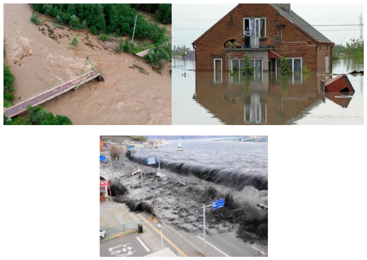
Figure 2.
Example of land cover maps used as input parameters for flood modelling.
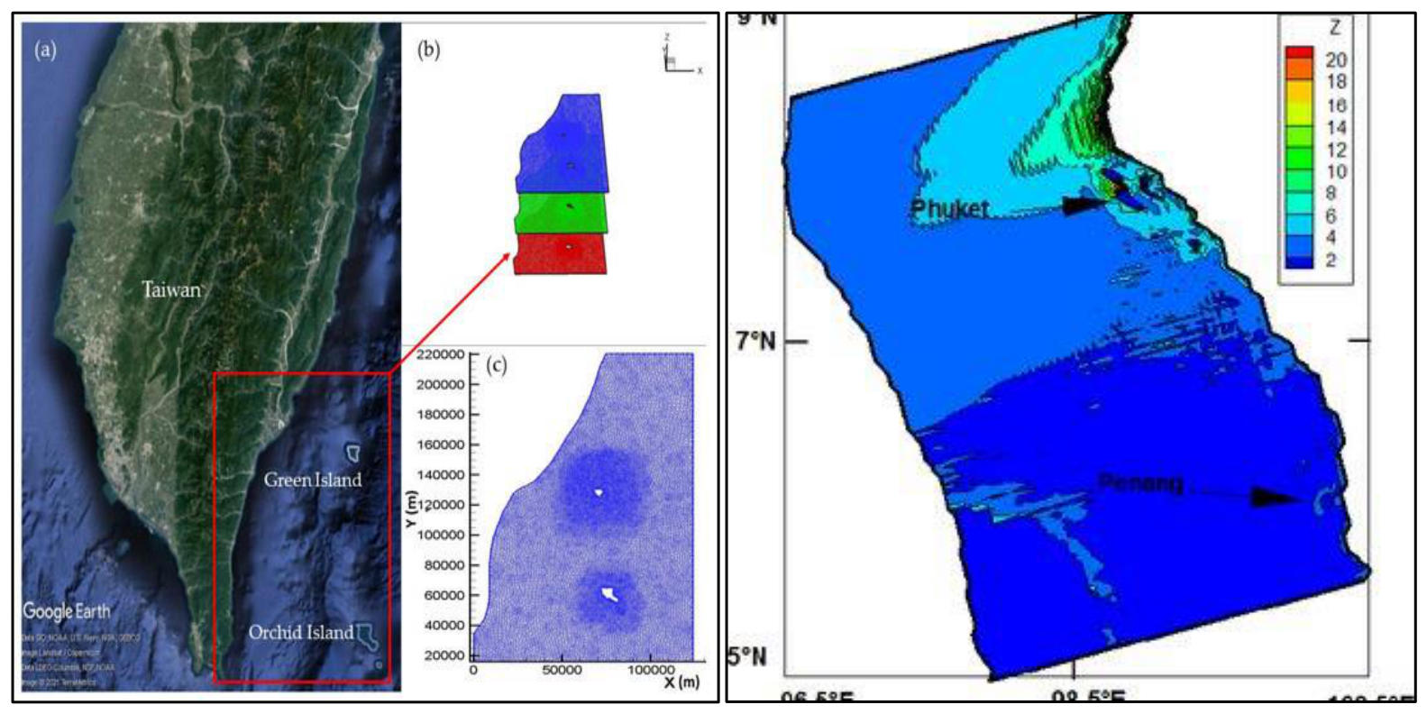
Figure 3.
Initial profile
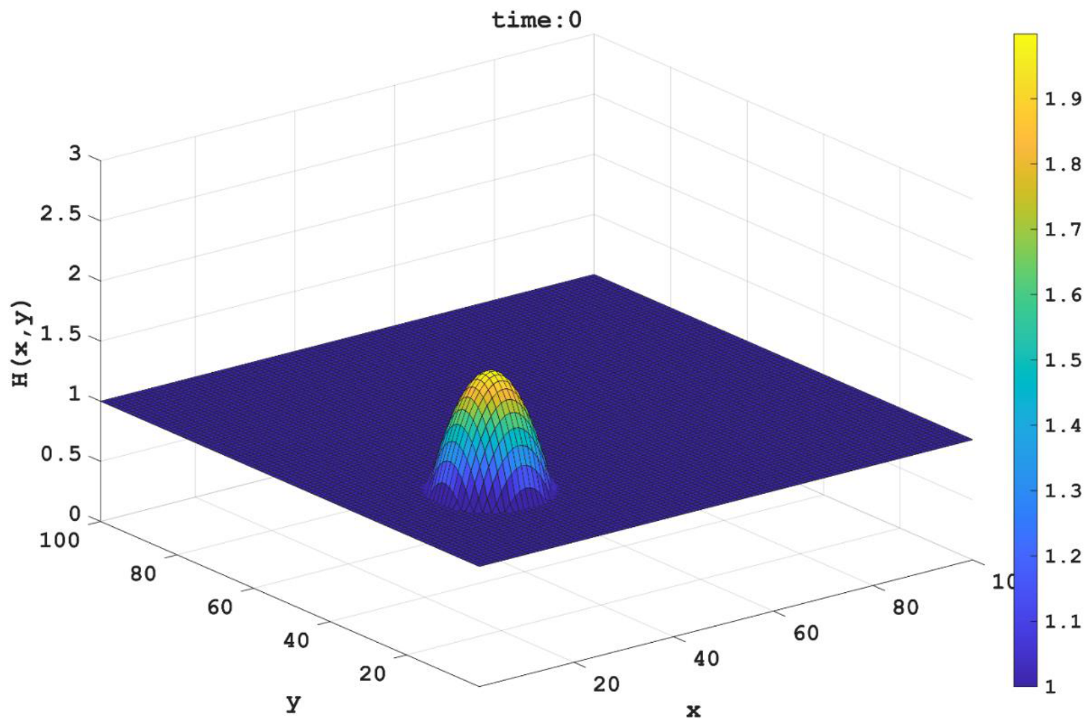
Figure 4.
Water depth profile, time
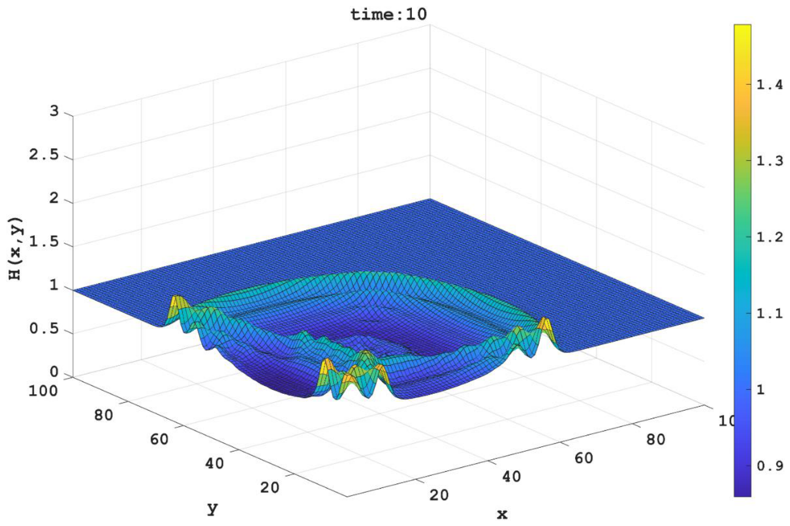
Figure 5.
Water depth profile , at a given time
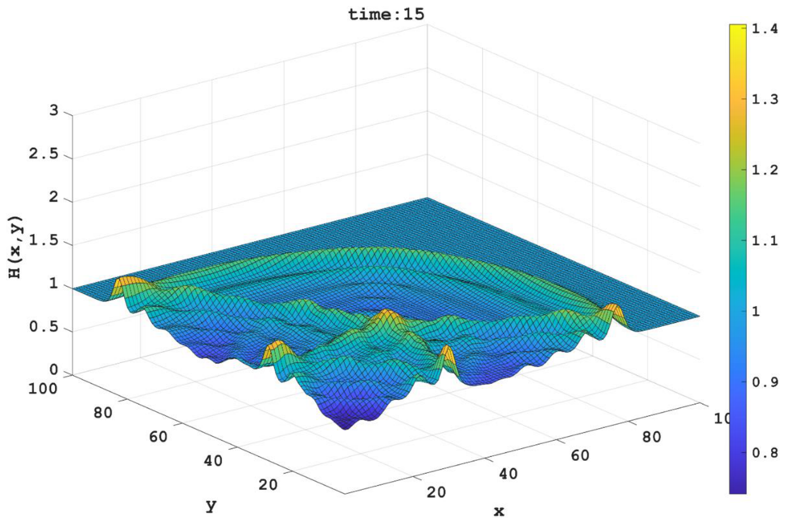
Figure 6.
Water depth profile , time
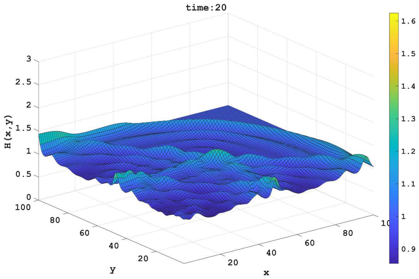
Figure 7.
Water depth profile , at the final time step, when
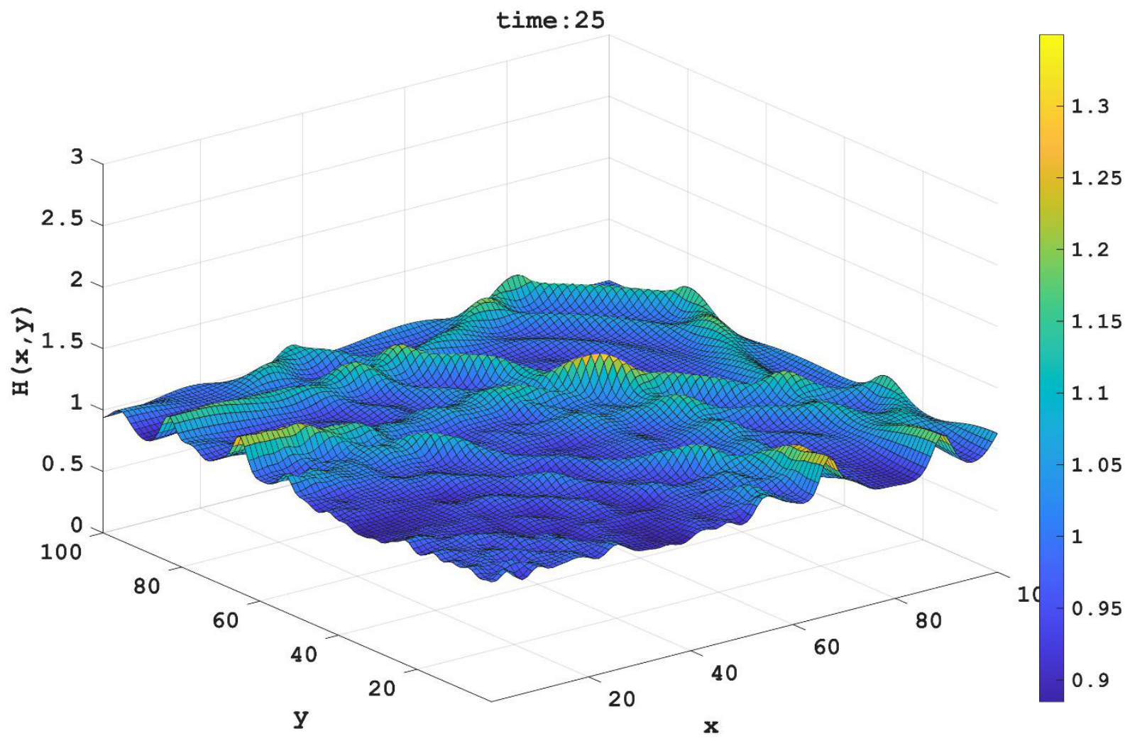

Table 1.
Summary table comparing the main current methods underlying the discretisation of shallow-water equations and used in modern oceanography.
Table 1.
Summary table comparing the main current methods underlying the discretisation of shallow-water equations and used in modern oceanography.
| Method Criterion |
Finite difference method | Finite volume method | Finite element method | Haloquin method and its modifications |
|---|---|---|---|---|
| Typical accuracy | 2nd order and above | 2nd order accuracy | 2nd order accuracy | usually 2nd order accuracy |
| Handling discontinuities | poor, as unnatural oscillations occur; the method requires artificial viscosity | excellent in the case of a conservative form | satisfactory | excellent, as it takes into account the physical naturalness of discontinuities |
| Complex geometries / Unstructured meshes | Poor, as it requires structured or block meshes | good | Best (maximum flexibility) |
best |
| Terrain processing | achieved using special methods | good | good | achievable, but difficult to implement |
| Flooding and drainage | problematic | good | Good – special Euler methods | good |
| Computational complexity | low | medium | medium or high | high |
| Main applications | oceanography, large-scale processes where velocity is critical | universal standard for rivers, floods, tsunamis | detailed modelling with complex geometry, channel processes | acoustics, high-precision problems where waves are important |
| Code example / Implementation | MITgcm, ROMS | ANUGA, LISFLOOD-FP (simplified), Basement | TELEMAC-2D, KratosMultiphysics (FIC-FEM) | Thetis, Secondo |
Table 2.
Analysis of finite difference methods in the study of complex processes in oceanography.
| Method | Main advantages | Main disadvantages | Typical application |
|---|---|---|---|
| Lax–Friedrichs, Lax–Wendroff and similar |
Highest speed, ease of implementation, work well for geostrophic balances | Poor approximation of complex geometry, discontinuity issues due to oscillations or scheme viscosity | Large-scale oceanography, regional models, problems where velocity is more critical than geometric details |
| Finite-difference methods with boundary approximation | Better accuracy on complex boundaries without grid refinement | More complex implementation, lack of full flexibility for unstructured grids | Models of lakes, reservoirs, and coastal zones with a sinuous shoreline |
| Meshless methods, such as the Galerkin method with modifications | High flexibility for complex geometry, high order of accuracy | High computational cost, complex implementation | Specialised problems requiring a combination of accuracy and handling of complex geometry, e.g., flow around obstacles |
| Finite differences for shallow water dispersion equations | Models wave dispersion, such as tsunamis, weaker stability conditions | Complex theoretical analysis, the problem of wave directional dependence in 2D | Modelling the transformation of tsunami waves and storm waves in deep water |
| Finite differences for kinematic waves | Extreme simplicity and speed | Very limited scope of application, do not work on complex terrain | Modelling of slope runoff, small catchments, initial approximations |
Disclaimer/Publisher’s Note: The statements, opinions and data contained in all publications are solely those of the individual author(s) and contributor(s) and not of MDPI and/or the editor(s). MDPI and/or the editor(s) disclaim responsibility for any injury to people or property resulting from any ideas, methods, instructions or products referred to in the content. |
© 2026 by the authors. Licensee MDPI, Basel, Switzerland. This article is an open access article distributed under the terms and conditions of the Creative Commons Attribution (CC BY) license (http://creativecommons.org/licenses/by/4.0/).
Copyright: This open access article is published under a Creative Commons CC BY 4.0 license, which permit the free download, distribution, and reuse, provided that the author and preprint are cited in any reuse.