
Submitted:
21 August 2026
Posted:
21 August 2026
You are already at the latest version
Abstract
Real-time quantum error correction requires a classical decoder to consume syndrome measurements at the rate the quantum hardware produces them, roughly one round per microsecond on supercon-ducting devices. The standard stability requirement is a utilization condition: the mean decode time per round must be less than the round period, ρ < 1. We show that this condition is inadequate for windowed decoders whose per-window cost grows superlinearly in the number of detection events, which is the empirical shape of matching-based decoders under burst-like syndrome content. For this class, stability is not a threshold but a basin. The deterministic backlog dynamics have a stable operating point and an unstable boundary B∗. Noise erodes that boundary downward, and sufficiently superlinear decoders escape spontaneously. In discrete-event simulations paired under common random numbers, a decoder with cost exponent γ = 1.5 and mean utilization ρ0 = 0.6 (forty percent nominal headroom) fails without provocation, with a mean time to failure of 1,344 ± 289 rounds, about 1.3 ms of wall clock at a 1 μs cycle. These Poisson times are upper bounds: modulating the arrival rate at fixed mean load shortens them monotonically with the measured dispersion index of the arrivals, fourfold by D ≈ 3, and a dispersion excess of twelve percent already uncensors the ρ0 = 0.5 ensemble. We measure the cost exponent of a production decoder (PyMatching 2, sparse blossom) and find it anisotropic: near-linear (γ ≈ 1.1–1.2) when a window grows in length at fixed syndrome density, but approximately quadratic (γ ≈ 2) when the same window grows denser. Bursts travel along the dangerous axis, where the basin is 2–4 rounds deep for ρ0 between 0.5 and 0.8. Spatially clustered event content, the syndrome footprint of leakage and cosmic-ray bursts, is worse still: at matched event count, clustered windows cost 7.6× length-grown ones and 4.8× uniformly densified ones, so the quadratic density exponent is a conservative proxy for burst content. The anisotropy is a property of the matching class rather than of one implementation, since a second exact-MWPM decoder reproduces the density exponent, while a BP+OSD decoder is nearly event-independent: no basin, but orders of magnitude more cost per window. The basin is the price of event-adaptive decoding. Greedy catch-up (“decode everything queued”) is precisely the divergent policy. A bounded decoding window restores stability, and the measured stability edge lands on a closed-form line. The rule survives finite memory: under greedy service a queue cap acts as an implicit window, and a cap on the unstable side of the same line pins at the cap and sheds rounds indefinitely, so adding buffer memory makes the greedy policy strictly worse. The simulation model is cross-validated against Stim at the level of individual fault mechanisms.
Keywords:
surface code
; real-time decoding
; minimum-weight perfect matching
; fault-tolerant quantum computing
; state-dependent queues
; stochastic stability
; correlated error bursts
; discrete-event simulation
1. Introduction
A fault-tolerant quantum computation is a race between two processors. The quantum hardware emits syndrome measurements on a fixed cadence, and a classical decoder must convert them into corrections fast enough for the computation to proceed. If decoding falls behind, corrections arrive too late to steer non-Clifford operations, the logical clock stalls, and the backlog compounds. This compounding is the backlog problem [1,2,17]. The condition usually stated for real-time viability is a utilization bound: the mean decode time per syndrome round must be below the round period, . Real-time decoding demonstrations state their stability case in exactly these terms, certifying against the mean per-round latency [17,19].
Our claim is that for an important class of decoding systems the utilization bound is the wrong condition. It is not merely conservative or approximate. It is structurally wrong, in the sense that it cannot distinguish systems that differ by orders of magnitude in reliability. The class is that of windowed decoders with superlinearly event-dependent cost: the decoder periodically takes a batch (window) of accumulated syndrome and pays a decode cost that grows faster than linearly in the number of detection events the window contains. Matching decoders have this shape in practice, and we measure it directly in Section 5.5.
Our contributions:
- 1.
- A basin, not a threshold (Section 2 and Section 5.1). For window-cost exponent , the deterministic backlog dynamics have two fixed points. The upper one, , is an unstable basin boundary that no mean-based analysis can see. At a single mean utilization () we exhibit four decoders spanning unconditional stability to spontaneous failure.
- 2.
- Noise erodes the boundary (Section 5.1). The stochastic system diverges at perturbations the deterministic map survives. The deterministic reference is drift-matched: its batch costs use the same Poisson moments as the stochastic system’s expectations, so the gap is fluctuation physics rather than a Jensen mean-inflation artifact. The analytic is therefore an unsafe provisioning line.
- 3.
- Spontaneous failure at nominal headroom (Section 5.2). At and , escape from the basin is driven by ordinary Poisson fluctuation alone. The measured MTTF is rounds, falling to at . The escape-time coefficient of variation is below one, so the failure is not memoryless, and MTTF alone under-describes it.
- 4.
- Greedy catch-up is the failure mode, and bounded windows are the fix (Section 5.4). With a per-window overhead, the per-round cost is minimized at small windows, and the measured stability cliff lands on the closed-form line . The intuitive recovery policy, taking everything queued, is the divergent one.
- 5.
- The exponent of a real decoder is anisotropic (Section 5.5). Sparse blossom is near-linear when windows grow in length and approximately quadratic when they grow in density. At matched event count, density-packed windows cost length-grown ones, and spatially clustered content, the blob-shaped syndrome footprint that leakage and cosmic-ray events actually produce [28,29], costs . Bursts deliver density, and clustered density is the worst case we measured. The anisotropy is a property of the matching class rather than of one implementation: a second exact-MWPM decoder reproduces the density exponent (), while BP+OSD is nearly event-independent, with no basin but orders of magnitude more cost per window (Section 5.6).
- 6.
- Dispersion sets the clock, and finite memory obeys the same line (Section 5.3 and Section 5.4). At fixed mean load, MTTF collapses monotonically with the measured dispersion index of the arrival process, independent of how the dispersion is produced, so the Poisson escape times are upper bounds. With a finite queue the bounded-window rule carries over unchanged: cap placement is the same closed-form decision, and the failure mode on the wrong side of it is permanent data loss rather than latency.
Methodologically, all simulations run on a verification-first discrete-event engine (Section 4). Its runs are reproducible from content-addressed identities, its state machines carry runtime-checked invariants, and its paired comparisons are audited at the level of random draws. The underlying circuit model is cross-validated against Stim [3] mechanism for mechanism. The cross-validation caught three defects that internal verification could not (Section 4.2).
2. Model: Windowed Decoding as a State-Dependent Queue
Syndrome rounds arrive deterministically, one per period T. All times are in ticks, with throughout, read as s per tick against a s cycle. Round r carries detection events. We use as the model’s reference rate; its physical anchoring is order-of-magnitude. Our cross-validated distance-3 memory at (Section 4.2) yields detection events per three-round shot, which is per round, while the distance-13 benchmark circuits of Section 5.5 carry () to () events per round on their much larger detector set ( at fixed p). Measured hardware brackets the same range: the detection probabilities reported for the Willow surface codes imply roughly to events per round at to 7 [17]. The value sits inside that physical range. Because is calibrated to a target utilization at whatever is chosen (see below), sets the granularity of fluctuations rather than the mean load, and burst sizes quoted in events should be read against the chosen . A 200-event burst, for example, is 125 round-equivalents at . The decoder serves the queue in windows: when free, it removes up to W queued rounds (greedy: ) as one batch and occupies itself for
where E is the total number of detection events in the batch. The one-tick floor matches the simulated machine, and the integer boundary matters for the entries of Table 1. Equation (1) is the declared cost model whose exponent Section 5.5 measures on a production decoder. We calibrate so that the steady-state single-round cost matches a target mean utilization: .
2.0.0.1. The deterministic map.
Under greedy windowing, a backlog of B rounds is served as one batch carrying events, and new rounds arrive during the service. The deterministic (mean-drift) reference evolves the backlog by the drift-matched map
Using the Poisson moment rather than the naive keeps the reference system at the same mean drift as the stochastic one. With the reference would run at a lower effective utilization by Jensen’s inequality, and part of any stochastic-versus-deterministic gap would then be a calibration mismatch rather than fluctuation physics. The correction is a few percent in the boundary region: the integer fixed points of Table 1 move by at most one round relative to the naive map, but the deterministic critical bursts of Figure 2 move by up to 20%.
For , f is affine with a single, globally attracting fixed point whenever . This affine case is the textbook condition, and the queueing-literate reader will recognize it as valid precisely for state-independent service, which is the assumption that superlinear event-dependent cost violates. For , f is convex and has two fixed points: a stable operating point and an unstable boundary . Any excursion beyond , whether a burst or an unlucky run of fluctuations, diverges permanently, in a system whose mean utilization may be far below one. Table 1 shows how shallow the basin becomes as grows.
Figure 1.
(a) The drift-matched backlog map, Equation (2), at . For the single fixed point is globally attracting. For the map is convex, and the open circles mark the unstable boundary , from which the backlog flows away in both directions (arrows); the callout marks the boundary, . (b) Basin depth versus mean utilization. At the same the basin spans two orders of magnitude across exponents that identical mean-throughput measurements cannot distinguish.
Figure 1.
(a) The drift-matched backlog map, Equation (2), at . For the single fixed point is globally attracting. For the map is convex, and the open circles mark the unstable boundary , from which the backlog flows away in both directions (arrows); the callout marks the boundary, . (b) Basin depth versus mean utilization. At the same the basin spans two orders of magnitude across exponents that identical mean-throughput measurements cannot distinguish.
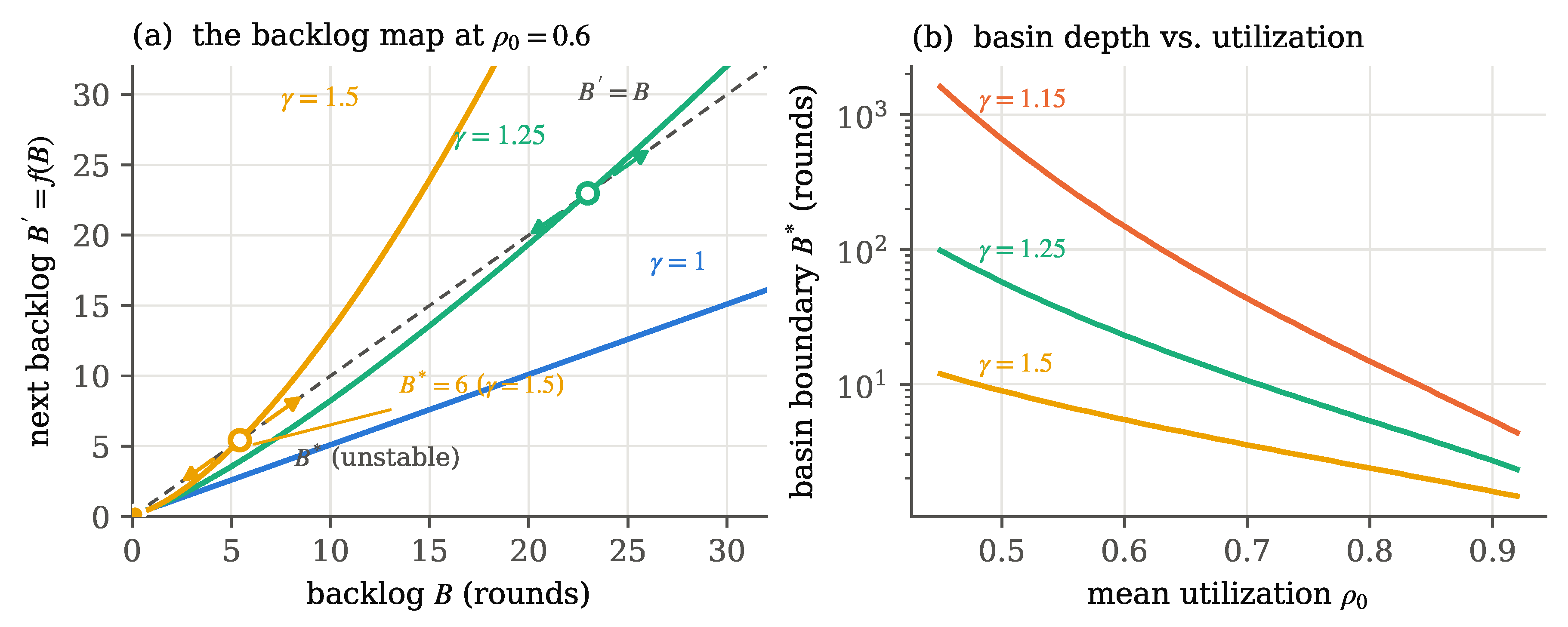
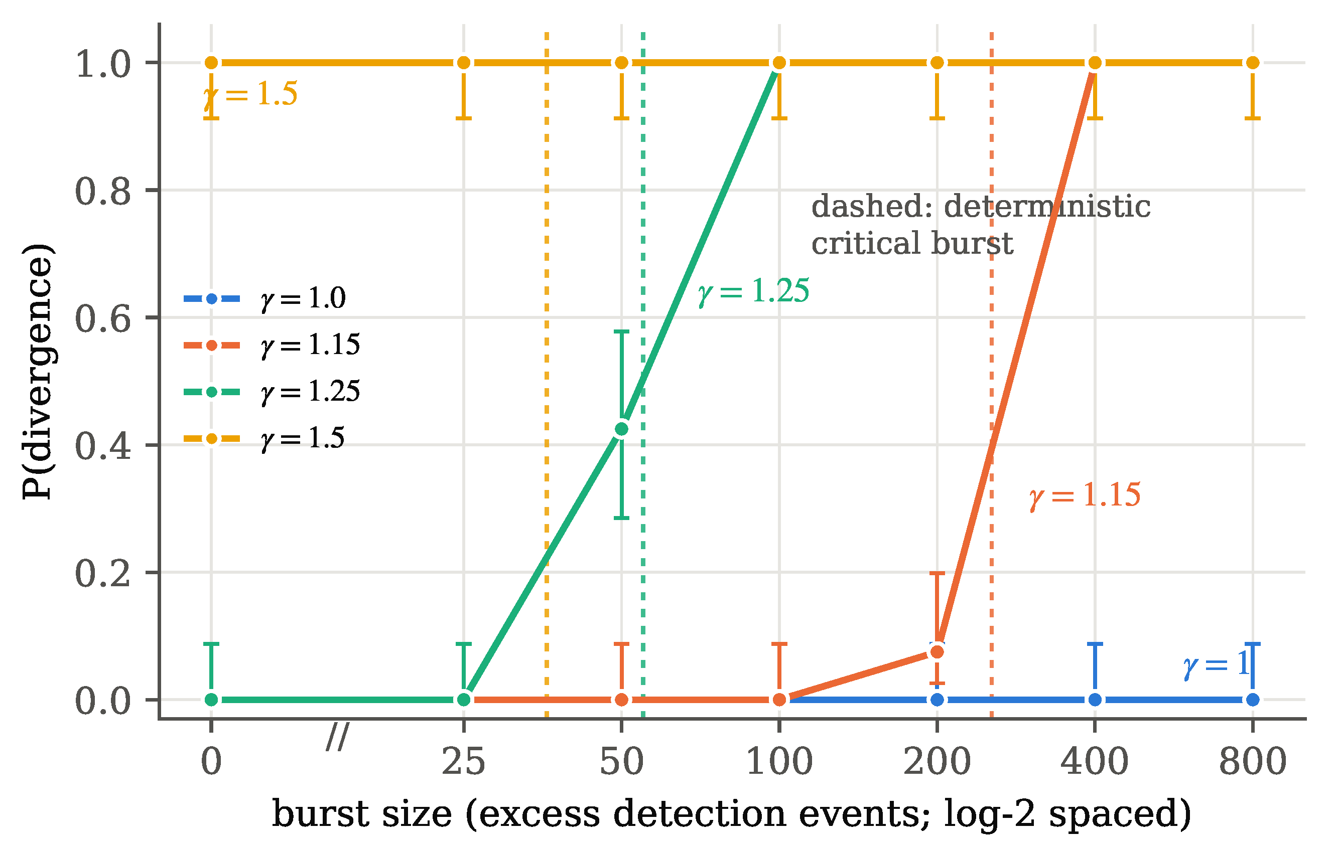
Figure 2.
Measured versus burst size at ( per point; Wilson 95% intervals), with each exponent’s deterministic critical burst as a dashed vertical line (bisection on the drift-matched noise-free dynamics). Every stochastic transition sits at or left of its deterministic line. Fluctuations carry the system over the boundary at perturbations the mean-field analysis survives, and requires no perturbation at all.
Figure 2.
Measured versus burst size at ( per point; Wilson 95% intervals), with each exponent’s deterministic critical burst as a dashed vertical line (bisection on the drift-matched noise-free dynamics). Every stochastic transition sits at or left of its deterministic line. Fluctuations carry the system over the boundary at perturbations the mean-field analysis survives, and requires no perturbation at all.
3. Related Work
Windowed decoding is as old as the surface code itself. Overlapping-window decoding appears already in Dennis et al. [8], and the modern real-time literature develops it into sliding-window and parallel-window architectures: Skoric et al.’s parallel window decoding [9], Tan et al.’s scalable window scheme [10], and Bombín et al.’s modular decoding [11]. Alongside these sit hardware decoders engineered for bounded latency, including LILLIPUT [12], Helios [13], and Barber et al.’s real-time collision-clustering decoder on FPGA [14]. The most complete demonstration to date is the real-time decoder of the Willow below-threshold experiment: streaming sparse blossom over ten-cycle processing blocks, with threads assigned to spacetime regions and fused asynchronously, holding a mean latency of s over cycles at against a s cycle [17]. Caune et al. integrate a sub-microsecond FPGA decoder directly into the control loop and report the backlog problem avoided, certified by mean per-round latency [19]. On the qLDPC side, Relay-BP targets real-time belief-propagation decoding of bivariate-bicycle codes [20], now demonstrated on FPGAs [21]; an iteration-bounded BP decoder caps its cost at an accuracy price, the same exchange Section 5.4 quantifies for windows. All of these architectures bound their windows by construction, historically motivated by latency and locality. Adaptive-window designs grow the window when decoder confidence drops [22]; expansion triggered by dense content is state-dependent service cost by construction, and without a bound equivalent to it reinstates the convex coupling of Section 2 at the moment expansion is most expensive. System-level analyses of the real-time stack identify round time and tail latency, rather than mean throughput, as the binding constraints [25].
Our single-server greedy queue is the base case whose pathology explains, in dynamical-systems terms, why bounding the window is not merely convenient but stabilizing: greedy catch-up is the divergent policy (Section 5.4), and a bounded window with removes the unstable fixed point entirely. The backlog problem itself is stated in Terhal’s review [1] and quantified by Smith et al. [2] at the utilization level. Our contribution is the structure below the utilization level.
The classical control side of the field is moving in a direction that makes this structure more binding, not less. HRL Laboratories has demonstrated a digitally controlled silicon quantum processing unit whose control electronics, including the syndrome-extraction sequencing for a distance-5 repetition code, run on a custom cryogenic CMOS controller inside the cryostat, with no real-time input from room-temperature equipment [16]. Decoding in that demonstration was a simple parity check evaluated offline. Section 6 returns to what the basin picture implies for decoders that must live within a cryogenic power budget.
On the queueing side, bistability and metastable congestion collapse in systems whose service degrades with state are classical subjects. Slotted ALOHA exhibits bistability [26], and loss networks exhibit metastability [27]; both show the two-fixed-point structure of Equation (2), and that community will recognize the convex one-dimensional map on sight. The new content here is the QEC instantiation: the identification of the decoder’s event-dependent cost as the state coupling, the measured anisotropy of that cost in a production decoder, and the resulting provisioning requirement. The excursion spectrum that drives escapes has direct physical referents. Cosmic-ray events produce catastrophic, spatially clustered error bursts in superconducting arrays [28], and leakage accumulates into correlated syndrome content [29]. On gap-engineered devices the measured spectrum has shifted but not vanished: the Willow repetition-code experiments observe correlated bursts about once per hour, localized to roughly 30 qubits, with detection probabilities elevated three- to six-fold and decaying over about s [17]. The residue has a measured mechanism: ionizing radiation transiently raises the quasiparticle density and produces correlated phase-error bursts lasting about a millisecond, which survive gap engineering [23]. All of these deliver exactly the dense, clustered windows that Section 5.5 measures as the most expensive per event. Correlated noise enters the decoding literature as an accuracy problem, because decoders built on independent-error models mismatch the true error distribution. The measurements of Section 5.5 give it a second consequence: clustered syndrome is also the most expensive content per event, so one physical footprint degrades accuracy and stability together.
4. Methods
4.1. Verification-First Simulation
All experiments run on polysim, a discrete-event simulation engine built around four disciplines that this study exercises end to end. First, every run is reproducible from a content-addressed identity (world hash, scenario hash, seed, replication index) and reproduces its journal digest byte for byte. Second, the simulated components are state machines with declared invariants checked on every transition; the decoder queue, for instance, carries machine-checked rules that its published backlog equals its actual queue and that a dropped round is a journaled refusal, never an omission. Third, paired comparisons run under common random numbers with a mechanical audit that the paired scenarios drew identical streams (every comparison below passed). Fourth, statistics that cannot be computed are refusals with named causes, never silently absent numbers. Across all runs reported in this paper the invariant monitors evaluated 21 declared rules per replication with zero violations.
Perturbations (bursts) are scheduled, not drawn, so the background noise realization is byte-identical across every scenario of a sweep. The exponent and calibration sweeps consume no random draws at all.
4.2. Cross-validation of the Circuit Model against Stim
The event rate and the burst semantics are grounded in a concrete code: a distance-3 rotated surface-code memory (9 data + 8 ancilla qubits, 3 rounds, ideal final readout) simulated by exact Pauli-frame propagation, with a generated layout, machine-checked schedules, and an exhaustive circuit-fault-distance proof used as a gate on all sampling experiments. The proof reproduces the known schedule-dependent fault-distance results, hook error witness included [5,6].
The model is cross-validated against Stim [3] at three levels. Structural: the single-fault symptom sets (which detectors fire, and whether the logical observable flips) of our mechanism table and Stim’s detector error model are identical, with 199 distinct symptoms for the good schedule and 213 for the bad one, and with per-symptom probabilities agreeing to 1.9%, the cross terms between channel composition and linear addition. Distance: Stim’s undetectable-logical-error search returns minimum weights 3 and 2, matching our proofs. Statistical: Stim shots decoded by our own lookup decoder give logical error rates 0.0283 / 0.0649 and detection fractions 0.0662 / 0.0657, each inside our engine’s own intervals (, , ).
The cross-validation caught three defects that internal verification (invariants, known-answer tests, reproducibility) could not have caught, and we consider this the methodological finding of the exercise: a physically non-deterministic detector definition invisible to a Pauli-frame simulator by construction, a silent gap in a fault table labeled “proved,” and a probe denominator off by exactly (Appendix A details all three). Internal verification bounds self-consistency; only an external referee bounds truth.
5. Results
5.1. Stability Is a Basin
Table 2 is the central result. Every cell has the same mean utilization (), the same arrival process, and the same scheduled burst profile (40 rounds, beginning at round 400 of 4,000). Only the cost exponent and the burst magnitude vary. Divergence is classified as more than 100 rounds of outstanding work at the horizon. Recovered runs end near zero, diverged runs end in the hundreds to thousands, and the indicator is itself a probe whose ensemble mean carries a confidence interval.
First, mean-based provisioning cannot distinguish these four systems. At identical their behavior spans unconditional stability ( absorbs a burst of the per-round load and recovers fully) to failure without provocation. Second, the stochastic boundary sits below the deterministic one, and because the deterministic reference is drift-matched, the gap is genuinely fluctuation-activated rather than a mean-calibration artifact. The drift-matched critical bursts (bisection on the dynamics of Equation (2); dashed lines in Figure 2) are 254, 55, and 36 events for , , and . Against these, diverges in 43% of runs at a burst of 50, below its deterministic critical burst of 55, and diverges in 8% of runs at 200, which is its deterministic critical burst. Provisioning against the analytic therefore still fails stochastically. Third, the sharpest cell is at zero burst: 100% divergence in a system whose deterministic map survives bursts up to 36 events. This failure is noise-activated escape from a metastable basin, and we quantify it next.
5.2. Spontaneous Escape Is Fluctuation-Driven and Sub-Exponential
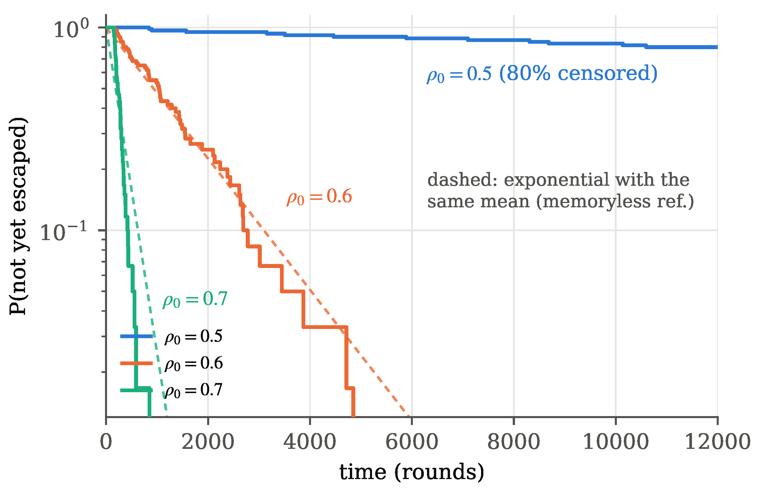
The failure rate is acutely sensitive to utilization, with a five- to forty-fold MTTF collapse per of . The measured step is ; the censored step is at least and, under any reasonable extrapolation of the censored row, plausibly around . The basin depth itself barely moves across the same range (Table 1), so the sensitivity lies in the escape rate, not the barrier position, as in thermal escape over a fixed barrier [7]. The total escape time’s coefficient of variation is consistently below one: escape is not memoryless. A provisioning methodology that quotes MTTF alone therefore under-describes the failure process, because the distribution’s shape matters.
Decomposing each escape path at the analytic boundary shows where the determinism lives. For each replication we record the first crossing of and the time from that crossing to the 100-round threshold. The waiting time to first crossing is memoryless in both ensembles ( at , at ; ), consistent with noise-activated escape. The breakout leg behaves differently at the two utilizations. At it is markedly narrower than exponential ( (sd) rounds, ), which is the wait-then-ramp picture. At , where is only 6 rounds, the first crossing is a weak committor: the backlog brushes the shallow boundary and re-enters many times before a decisive excursion, so the first-crossing decomposition stays memoryless () even though the total escape time is sub-exponential (). For basins this shallow, no single backlog level cleanly separates waiting from breakout. The sub-exponential total is the signature that does not depend on that choice.
Figure 3.
Escape-time survival curves at , no perturbation ( each; the curve is right-censored at the horizon). Dashed: exponential references with the matching means. The measured curves are convex relative to memoryless decay, with few early escapes and then a faster-than-exponential fall. This shape is the CV signature of a waiting time followed by a near-deterministic breakout.
Figure 3.
Escape-time survival curves at , no perturbation ( each; the curve is right-censored at the horizon). Dashed: exponential references with the matching means. The measured curves are convex relative to memoryless decay, with few early escapes and then a faster-than-exponential fall. This shape is the CV signature of a waiting time followed by a near-deterministic breakout.
5.3. Dispersion Sets the Clock
The escape times above assume Poisson arrivals, dispersion index . Measured devices are overdispersed: detection-event rates show unexplained spikes [16] and burst phenomenology at every timescale [28,29]. To measure what dispersion alone does to the clock, we modulate the arrival rate with a scheduled square wave, alternating between with half-period rounds and a per-replication phase offset, and recalibrate against the modulated stationary moment, , so the mean load is held fixed and the experiment varies dispersion without varying drift (the same Jensen discipline as Equation (2)). The achieved dispersion is measured per arm, as the variance-over-mean of event counts in 100-round windows, rather than derived. The baselines are common-random-number re-runs of Table 3 and reproduce it exactly.
Three findings follow (Table 4, Figure 4). First, MTTF collapses monotonically with measured dispersion at fixed mean load: fourfold by at , sevenfold by . The effect is largest where the headroom is largest: a twelve percent dispersion excess () already lifts the escape probability from 20% to 67%, and by the previously censored ensemble escapes every time, at least fourfold below its censored median. Second, dispersion is the right axis: the and series fall on a single MTTF-versus-D curve, so the modulation period matters only through the dispersion it produces. Third, the escape-time CV stays below one throughout but falls with dispersion, to about at high D. Strongly modulated arrivals therefore make failure more deterministic rather than more memoryless: the system dies on the first sufficiently adverse high-rate phase, and the wait for one is narrow. For provisioning, the Poisson row of Table 3 is the best case at its mean load, and the correction for a device’s measured D is a multiplicative MTTF collapse read off Figure 4.
5.4. Greedy Catch-Up Is the Failure Mode
With a realistic per-window overhead ( of the 10-tick budget), the per-round cost of a width-W window, with , is minimized at small W. Overhead dominates tiny windows, and the superlinear term dominates large ones. This section operates at and , a drift-matched single-round steady cost of 7.9 ticks (). This is deliberately hotter than the used elsewhere, in order to place the window sweep across the stability line. For bounded W the map is asymptotically affine in B with slope below one whenever , so bounding the window removes the upper fixed point entirely. There is no basin boundary to fall over, and stability is global. Greedy windowing is what restores the convexity and, with it, the basin.
The condition is necessary for stability but is not a performance guarantee. As the drain rate vanishes and the recovery time after a burst diverges even on the stable side. Table 5 shows both regimes. Windows of 2–8 rounds absorb a 200-event burst with single-digit mean backlogs. The window sits almost exactly on the line ( against ): it is stable in the strict sense, with no upper fixed point, but its post-burst drain is about 0.1 tick per round, and the “90%” entry is the more-than-100-outstanding-at-horizon classifier firing on a slow transient. A re-run at a -round horizon () confirms the distinction. The backlog peaks near 353 rounds and is draining by the horizon (ensemble mean 209, final 176), with 60% of replications still above the 100-round line; this behavior is slow recovery. The window , with , grows without bound (final backlog near 5,400 and rising); this growth is instability. The two regimes call for different remedies: more margin in the first case, a different window in the second. The greedy policy, taking everything queued, which is the intuitive recovery move, diverges always, with a mean backlog three orders of magnitude above the bounded optimum.
The quantity is a throughput criterion, and the optimum it selects ignores accuracy. Short windows harm matching accuracy at window boundaries, which is why practical designs use overlapping or fused windows of order the code distance, and why real-time operation carries a measured accuracy cost ( in real time versus offline in the Willow experiment [17]). It therefore selects among accuracy-admissible windows; it does not license windows below the accuracy floor.
5.4.0.2. Finite memory.
The queue above is unbounded, so escape manifests as latency. A decoder co-located with control hardware has a hard queue bound, and the failure mode becomes data loss: a round arriving at a full queue is dropped (drop-newest here, as a journaled refusal, never an omission). The design question is where the cap C may sit, and the answer is the same closed-form line. Under greedy service a cap is an implicit window bound: with C on the stable side of , every excursion is a bounded loss episode followed by full recovery, and the loss under the standard burst is essentially the burst overshoot above the cap. With C in the unstable range, the queue pins at the cap and sheds rounds indefinitely, a saturated, permanently lossy state, and more memory makes greedy strictly worse: at the greedy policy sheds the rounds it does at (Table 6). A bounded window is immune by construction: never saturates at any cap, and its loss vanishes once the cap clears the excursion peak (4.5 rounds dropped at under the burst, zero without it). A second regime appears under hotter load. In the escape configuration of Section 5.2, where even , a cap of 8 is too small to pin for 1,000 consecutive rounds, and the queue runs instead as a lossy governor, shedding a steady ≈2% of rounds forever, converting instability into chronic data loss rather than latency. For the hardware question of how much memory the decoder queue needs, the rule is: enough for the excursion spectrum’s overshoot above the operating point, and never a cap whose implicit window lands on the unstable side of .
5.5. The Measured Exponent of a Production Decoder Is Anisotropic
The cost model (1) was declared; this section measures it. PyMatching 2 (sparse blossom [4]) decodes Stim-generated rotated-surface-code windows (). Decode time for individual shots, stratified by detection-event count and timed as a minimum over repeated calls, is regressed against events, with fitted by grid search (closed-form least squares in at each candidate , SSE on linear time) and reported with a 5%-SSE band. Because a three-parameter power law trades against at the low-E end, we re-fit with pinned to an extrapolation as a robustness check. The exponents move from 1.14 to 1.16 (window) and from 2.31 to 2.05 (density), so the anisotropy is not a fit degeneracy.
The exponent depends on how the events arrive:
- Window axis (the window grows in rounds at fixed density, which is ordinary catch-up): –, bands across passes, . Near-linear.
- Density axis (fixed 40-round window, syndrome packed denser by raising p): , bands spanning across passes, . Approximately quadratic.
- Cluster axis (fixed window, fixed background , with the k detectors nearest a random space-time center flipped, the syndrome footprint of a localized burst [28]): a global power-law fit is poorly conditioned here, because decode time at fixed E varies severalfold with blob location (boundary versus bulk), so we report the matched-event form below.
- Matched-event check (robust to the thermal drift that moves the absolute fits; all three axes measured adjacently in one process): at 600–900 events, density-packed windows cost length-grown ones (1.52× in an earlier pass), and clustered windows cost length-grown ones, which is the uniformly densified windows at the same event count.
The mechanism is consistent with the algorithm’s structure. In blossom-type matching, growing the window in length adds graph volume while defect interactions stay local, whereas packing defects closer multiplies alternating-tree and blossom interactions per defect. That is a plausible route to near-quadratic scaling, and clustering then concentrates the interactions in one region. In Figure 5, the density series’ larger intercept (about 80 s versus about 20 s at small E) reflects the fixed 40-round graph paying its size at low occupancy, while the window series builds small graphs at small E. At matched E the two sweeps also differ in graph size (a 160-round sparse window versus a 40-round dense one), so the ratio folds together density and graph-size effects. The cluster series, which holds both the graph and the background fixed, isolates content structure, and it is the cleanest evidence that burst-shaped syndrome is intrinsically expensive.
Mapping the measured exponents through Equation (2) gives Table 7, where and are the two independent passes’ point estimates and is the upper edge of the pooled 5%-SSE band. Steady-state catch-up sits in a deep basin, thousands of rounds at . But within the window-axis confidence band alone, at ranges from effectively infinite to 11 rounds: real-time provisioning requires pinning the cost exponent to about , a requirement we have not seen stated anywhere in the literature. Burst content, on the density axis, faces a basin of 2–4 rounds for between 0.5 and 0.8. A sparse-blossom-class decoder provisioned on its steady-state throughput curve therefore meets bursts on a cost curve two exponent classes worse, and the cluster measurement says even that is the optimistic reading.
On this machine, single-core per-round decode time corresponds to (, ) up to () against a s cycle. One core cannot hold real time at all, which is why real systems window and parallelize, and why the windowing policy is the operative lever. This does not contradict the published sparse-blossom throughput of roughly s per round at and [4]. That figure is batched C++ throughput, while ours is per-call invocation through the Python boundary, whose constant lands in and whose per-shot dispatch forgoes batching. Per-call is the operationally relevant mode for real-time windowing: a window must be decoded when its deadline arrives, not when a batch fills.
5.6. The Anisotropy Is a Property of the Matching Class
Everything above measures one decoder. To test whether the anisotropy is a property of PyMatching or of its class, we ran the same three axes over three more decoders (Table 8): fusion-blossom, a second exact-MWPM implementation whose own empirical claim is near-linear scaling; the ldpc package’s union-find decoder; and BP+OSD as an intended superlinear control. Accuracy differences across decoders are out of scope, since this measures cost shape only.
Three conclusions follow. First, the anisotropy generalizes across the matching class. Fusion-blossom reproduces the density exponent with the tightest density band in this paper (, ), though its anisotropy expresses differently: a higher window exponent (1.49) and no matched-E density premium, but a clustered premium of . The density-to-window exponent gap, which is the quantity the basin analysis depends on, survives the implementation change. This pass also re-reproduces PyMatching’s own numbers within the earlier bands, a third consistency check on Section 5.5’s fits. Second, the software union-find decoder is not credibly fit by a power law at all, but its matched-E ratios are decisive: dense content costs and clustered content its own length-grown windows, at absolute times (0.1–6.8 s per window) nowhere near real time. We scope this to the measured implementation (matrix-inversion union-find in software); it says nothing about hardware collision-clustering decoders [14], which would need the same three-axis measurement on their own silicon. Third, the intended positive control refuted its prediction, and the refutation completes the taxonomy. BP+OSD’s cost is set by the graph and not by the events: the window exponent is 0.97 (pure graph growth), and denser windows are cheaper per event ( at matched E). For BP-class decoders the utilization condition is therefore approximately valid, because there is no event-dependent feedback to build a basin, but that validity is bought at a per-window cost of PyMatching’s and fusion-blossom’s at matched event count (≈640 ms for a 160-round window here). The taxonomy is then: matching-class decoders are cheap on average and metastable under bursts, and BP-class decoders are stable by construction and unaffordable per window. The basin is the price of event-adaptive decoding, and a provisioning methodology must know which side of that trade its decoder sits on.
6. Discussion
For windowed decoders with superlinearly event-dependent cost, report the basin, not the utilization. A provisioning claim should state (i) the measured cost exponent on both axes with a confidence band; (ii) the implied at the operating utilization; (iii) the expected excursion spectrum, that is, burst sizes and rates from the device’s leakage and radiation environment, for which measured magnitudes exist [17,23,28,29]; and (iv) the window bound W placing safely below the round period, with margin, since the recovery time diverges as even on the stable side. Items (i) and (iv) are a measurement and a design choice, item (ii) is closed-form, and item (iii) is the one input this paper takes from outside. The newest decoder implementations already report worst-case rather than mean latency [24], the reporting posture that items (i) through (iv) systematize. Parallel-window architectures [9,10,11] satisfy (iv) by construction; this paper supplies the dynamical-systems reason that the construction is load-bearing. Code class moves the exponent as well: noise-biased cat-qubit architectures suppress bit-flips passively and reduce active correction to a repetition code [18], whose quasi-one-dimensional matching graph should sit near on all three axes, placing that architecture, pending measurement at its operating density, in the unconditionally stable row of Table 1. The basin is a property of the code and decoder pair, not of quantum error correction as such.
The Willow below-threshold experiment is the existence proof that the mitigation regime is practical [17]. Its real-time decoder never executes greedy catch-up: syndrome is processed in bounded blocks and fused asynchronously, a working instance of the bounded-window rule, and it holds its mean latency constant over a million cycles at . The same data shows the tail our analysis predicts: infrequent latency spikes above ms, roughly nine hundred cycles of outstanding work, absorbed and drained on the stable side. The spontaneous failures of Section 5.2 are a property of the greedy policy class, not a prediction about deployed systems that already bound their windows. The open question is margin, not existence. Syndrome volume grows quadratically with distance and decoder latency grows with code size, as that experiment’s own outlook notes, and the basin accounting above is the instrument for deciding how much margin the next factor of requires. A burst of the magnitude and duration measured above carries roughly to excess detection events, so real excursions do not probe the edge of any basin in Table 2; they overrun it outright. Surviving them is therefore entirely a question of the drain rate against a once-per-hour recurrence, which is Section 5.4’s regime.
HRL Laboratories has reported a digitally controlled silicon quantum processing unit: a 54-dot array configured as up to 18 exchange-only spin qubits, operated entirely by a custom cryogenic CMOS controller inside the cryostat, executing a distance-5 repetition code over hundreds of autonomous syndrome-extraction rounds with sub-microsecond operations [16]. That demonstration solves, at the chip level, exactly the half of the real-time problem this paper takes as given: syndrome generation and control at rate, with all control signals generated inside the cryostat. Readout in that system is still digitized at room temperature, and decoding was a simple parity check evaluated offline; real-time decoding at error-correction speed remains open on that platform. Wherever the future decoder lands, the constraint is the same. On the room-temperature side it inherits the latency of the link that carries the syndrome out of the refrigerator. Inside the cryostat it inherits a hard power and area budget (the reported controller draws W at K), and a cryogenic decoder cannot buy its way out of a backlog excursion with burst compute, because the compute ceiling is fixed at design time. In that regime the windowing policy is not one lever among several; it is the lever. The provisioning discipline above then becomes a design input, since nothing can be added after the cryostat closes. The demonstration also shows that sub-microsecond operation is no longer specific to superconducting hardware, so the round period in our model should be read as a platform parameter rather than a superconducting constant.
Two features cut against intuition. Greedy catch-up, the natural recovery behavior and the default of any decoder that simply processes what has accumulated, is exactly the policy that converts a transient overload into a permanent one. And the deterministic basin boundary, though closed-form and correct as far as it goes, is not a safe engineering line: fluctuations carry the system over it from below, at rates our escape-time measurements quantify.
What this model deliberately omits marks the next experiment. The feedback studied here is computational: backlog leads to costlier windows. The physical feedback, in which a stalled logical clock idles qubits and raises the syndrome density the decoder then faces, compounds along the measured density axis, which is the quadratic one. The HRL experiment measures this ramp directly: without leakage-reduction units the detector event fraction grows steadily with syndrome round, and only their inclusion holds it stationary [16]. In our terms, leakage mitigation is what keeps constant; its absence hands the decoder a rising under which the operating point and the basin boundary drift toward each other and annihilate.
We measured this open-loop half of the coupled feedback directly, with a scheduled ramp at fixed service calibration (Figure 6). Two closed-form clocks bound the deterministic death: , where the single-round drift reverses, and , the saddle-node round where the map loses its fixed points. The deterministic system dies a fixed ≈143 rounds after across the decade of in which both clocks are defined, which is the intrinsic superlinear runaway time and a constant of the decoder rather than of the ramp. The dynamic saddle-node ghost scaling never engages, because the classification threshold sits two orders of magnitude above the ∼1-round tangency backlog. The stochastic system does not wait for either clock: it dies 303 rounds early at , 6,100 rounds early at , and at , where no extinction exists inside the horizon at all, every replication still fails, which is the moving-boundary form of the unsafe analytic boundary. The control arms carry the sharpest result: a constant rate equal to the ramp’s time-average kills the system sooner at every slope, by factors from to , because the ramp spends its early life benign while the constant arm runs hot from round zero. Neither the time-averaged utilization nor stationarity alone predicts the failure epoch. The load trajectory does, and provisioning against a drifting rate must integrate it. The remaining closed-loop half, in which the stalled clock itself raises , requires connecting the queue back into the circuit-level noise model, which our simulation framework supports but this paper does not yet exercise.
7. Limitations
The cost curve (1) is a declared model. The primary calibration (Section 5.5) measures one decoder (PyMatching 2.4.0), on one machine (a laptop-class x86 core), for one code family, with the Python call boundary contributing a constant to . The class comparison (Section 5.6) adds three software implementations under the same conditions, of which the union-find entry should not be read as representative of hardware union-find decoders, and all four exclude decoding accuracy from scope. The density-axis exponent moves by roughly with thermal state, and the matched-event ratio is the stable form of that claim. The cluster measurement flips detectors in a space-time ball, the syndrome footprint of a localized burst, rather than simulating a microscopic burst mechanism; it isolates what blob-shaped syndrome costs the matcher, not how a specific physical event produces it. The cost model applies to decoders whose batch grows with backlog: per-call windowed invocation, catch-up after stalls, and adaptive-window designs. Streaming architectures that hard-cap the decode problem on a constant-size graph buffer [17] have already applied the mitigation of Section 5.4; for them the state dependence moves into queueing delay rather than service cost, and they inherit the slow-recovery regime rather than the basin. The model’s event rate is an order-of-magnitude anchor between the measured distance-3 rate (0.53/round) and the benchmarked distance-13 rates (2.6–5.2/round), and it is treated as backlog-independent. The arrival process is Poisson with independent rounds except where Section 5.3 deliberately modulates it. Measured devices show correlated fluctuations, including unexplained spikes in detection-event rates on a silicon platform [16] and catastrophic correlated bursts on superconducting ones [28], and Section 5.3 turns the resulting caveat into a measurement: the Poisson MTTFs of Table 3 are upper bounds, and a dispersion index near 3, well inside reported device behavior, costs fourfold at . The square-wave modulation is one dispersion mechanism among many, and a device’s measured D enters through Figure 4 only to the extent that MTTF depends on D alone, which we verified across two modulation periods but not across mechanisms. The finite-buffer study fixes drop-newest semantics; a drop-oldest queue loses different rounds with different logical-error consequences, and the logical cost of a dropped round is outside the queue model’s scope, since we count rounds and not logical errors. The ramp study holds fixed while rises, so the decoder is not re-provisioned mid-drift. Divergence is classified against a declared threshold (100 outstanding rounds) at a declared horizon. This classifier flags slow recovery as well as true instability, and Section 5.4 disambiguates the two by horizon-doubling where it matters. The escape-time probe shares the same threshold by construction. The escape row is right-censored at the simulation horizon. The distance-3 circuit model, not the queue, is what the Stim cross-validation covers; the queue model’s external referent is the decoder benchmark. Sampling grids use –60 replications per cell. Sequential stopping was not applied to the basin grids, and the sharp 0/100 cells are limited by that n accordingly.
8. Conclusions
For windowed decoders whose cost grows superlinearly in syndrome content, real-time stability is a basin, not a threshold. The utilization bound cannot separate systems that differ by orders of magnitude in reliability: at a single mean utilization we exhibit decoders spanning unconditional stability to spontaneous failure, show that fluctuations carry the system over a drift-matched boundary the mean-field analysis survives, and measure the failure clock at ms of wall time with forty percent nominal headroom. The exponent that controls all of this is a measurable property of a real decoder, and it is anisotropic: bursts meet sparse blossom on a cost curve two exponent classes worse than steady-state catch-up, and clustered burst content is more expensive still. The design consequence is to bound the window, place below the round period with margin, and report the basin alongside the utilization.
Four further measurements place the framework against conditions a device actually presents. Arrival dispersion at fixed mean load collapses the escape clock monotonically with the measured dispersion index, sevenfold by , so the Poisson escape times are upper bounds and a device’s measured D enters provisioning directly. A drifting arrival rate kills the system before either closed-form clock, and a constant rate at the ramp’s time-average kills it sooner still, so the load trajectory rather than its mean sets the failure epoch. The anisotropy survives a change of implementation and separates the decoder classes: matching-class decoders are cheap on average and metastable under bursts, while BP-class decoders are stable by construction and unaffordable per window. Finite decode memory converts escape from a latency failure into a data-loss rate, and under greedy service more memory is strictly worse.
Three directions remain open. The exponent taxonomy should widen further still: union-find and clustering decoders on hardware, and the quasi-one-dimensional repetition strips of noise-biased architectures [18] at their operating densities, plausibly occupy the stable row of Table 1 and should be measured there. Neural decoders belong in the same taxonomy and sit at its stable end by construction: a network with fixed input dimension and constant-time inference does bounded work per window, which is the row [15]. Hybrid designs qualify that placement, since a pre-decoder that routes hard instances to a matching fallback [24] inherits the matching exponent on precisely the dense windows that trigger the fallback, and its effective exponent follows the fallback path rather than the fast one. Dispersion enters here too, since the square-wave modulation of Section 5.3 is one mechanism among many and a device’s own excursion spectrum may not reduce to a single index. And the loop this paper left open, a stalled logical clock raising the syndrome density the decoder then faces, closes through the circuit-level noise model along the quadratic axis. The direction of the hardware gives these measurements their urgency: as classical control moves into the cryostat and compute ceilings become design constants, the basin stops being an operational tuning concern and becomes an input to the machine’s blueprint.
Data Availability Statement
The results in this paper occupy three tiers of reproducibility. The deterministic results (Table 1 and Table 7, the and columns of Table 5 and Table 6, the ramp clocks of Figure 6, and the critical bursts of Figure 2) are closed-form consequences of Equation (2) and the constants stated with each table, and can be recomputed from this paper alone. The decoder measurements (Section 5.5 and Section 5.6, Figure 5, Table 8) depend only on open tools (Stim, PyMatching, fusion-blossom, ldpc); the benchmark script and the measured points behind Figure 5 accompany this paper as a standalone artifact. The stochastic simulations (Table 2, Table 3, Table 4 and Table 5 and Table 6, Figure 3, Figure 4 and Figure 6) were produced on polysim, a proprietary discrete-event engine. Within it, every run is addressed by a content-addressed identity (world hash, scenario hash, seed 20260817, replication index) and reproduces its journal digest byte for byte; paired comparisons carry a machine audit that scenarios consumed identical random streams; probes and their thresholds are content-hashed into each experiment’s identity. The per-replication outputs behind those tables and figures (divergence indicators, escape times, breakout decompositions) accompany this paper as data files, and the queue model is specified completely by Equations (1) and (2) together with the parameters listed in each section, so it can be reimplemented in any discrete-event simulator.
Appendix A. The Three Cross-Validation Defects
Each defect below survived the engine’s internal verification (21 machine invariants evaluated per replication, known-answer tests, byte-exact journal reproducibility) and was caught only by the external cross-validation against Stim.
(a) Physically non-deterministic detectors.
A boundary-plaquette mirroring in the layout generator produced a collision-free, invariant-clean circuit whose detectors compare measurements that are not deterministic in the absence of errors. A Pauli-frame simulator is constitutively unable to see this failure class: it tracks deviations from a reference execution it never checks, so a detector that is broken in the reference looks exactly like a working detector with a relabeled baseline. Stim’s structural comparison (which detectors fire for which fault) exposed it immediately.
(b) A silent gap in a table labeled “proved.”
The fault enumeration used one schedule variant’s gate slots when enumerating both variants, leaving mechanisms of the second schedule unenumerated. The gap was invisible to internal consistency checks because the enumeration is itself the reference the checks run against. The cross-validation’s symptom-set equality (199 and 213 distinct symptoms) failed until the enumeration was made schedule-dependent.
(c) A denominator off by exactly 24/20.
A detection-fraction probe divided events over the machine’s 20 detector components rather than the 24 syndrome bits of the readout convention. The defect was found because Stim’s detection fraction refused to match ours by a suspiciously clean ratio. Ratios of small integers in a discrepancy are a fingerprint of denominator disagreement, not physics.
References
- Terhal, B. M. Quantum error correction for quantum memories. Rev. Mod. Phys. 2015, 87, 307. [Google Scholar] [CrossRef]
- Smith, S. C.; et al. Managing classical processing requirements for quantum error correction. arXiv 2024, arXiv:2406.17995. [Google Scholar]
- Gidney, C. Stim: a fast stabilizer circuit simulator. Quantum 2021, arXiv:2103.022025, 497. [Google Scholar] [CrossRef]
- Higgott, O.; Gidney, C. Sparse Blossom: correcting a million errors per core second with minimum-weight matching. arXiv 2023, arXiv:2303.15933. [Google Scholar]
- No more hooks in the surface code: distance-preserving syndrome extraction for arbitrary layouts at minimum depth. arXiv 2026, arXiv:2603.01628.
- Improved methods for determining quantum error correcting code performance and fault tolerance. arXiv 2026, arXiv:2607.27153.
- Kramers, H. A. Brownian motion in a field of force and the diffusion model of chemical reactions. Physica 1940, 7, 284. [Google Scholar] [CrossRef]
- Dennis, E.; Kitaev, A.; Landahl, A.; Preskill, J. Topological quantum memory. J. Math. Phys. 2002, 43, 4452. [Google Scholar] [CrossRef]
- Skoric, L.; Browne, D. E.; Barnes, K. M.; Gillespie, N. I.; Campbell, E. T. Parallel window decoding enables scalable fault tolerant quantum computation. Nat. Commun. 2023, 14, 7040. [Google Scholar] [CrossRef] [PubMed]
- Tan, X.; Zhang, F.; Chao, R.; Shi, Y.; Chen, J. Scalable surface-code decoders with parallelization in time. PRX Quantum 2023, arXiv:2209.092194, 040344. [Google Scholar] [CrossRef]
- Bombín, H.; Dawson, C.; Liu, Y.-H.; Nickerson, N.; Pastawski, F.; Roberts, S. Modular decoding: parallelizable real-time decoding for quantum computers. arXiv 2023, arXiv:2303.04846. [Google Scholar]
- Das, P.; Locharla, A.; Jones, C. LILLIPUT: a lightweight low-latency lookup-table decoder for near-term quantum error correction. ASPLOS 2022, arXiv:2108.06569. [Google Scholar] [CrossRef]
- Liyanage, N.; Wu, Y.; Deters, A.; Zhong, L. Scalable quantum error correction for surface codes using FPGA, QCE 2023. arXiv arXiv:2301.08419.
- Barber, B.; et al. A real-time, scalable, fast and resource-efficient decoder for a quantum computer. Nat. Electron. 8 2025, arXiv:2309.0555884. [Google Scholar]
- Bausch, J.; Senior, A. W.; Heras, F. J. H.; et al. Learning high-accuracy error decoding for quantum processors. Nature 2024, 635, 834. [Google Scholar] [CrossRef] [PubMed]
- Members of the HRL Quantum Team and Collaborators, A digitally controlled silicon quantum processing unit. Nature 2026, arXiv:2604.16216655, 1154. [PubMed]
- Google Quantum AI and Collaborators, Quantum error correction below the surface code threshold. Nature 2025, arXiv:2408.13687638, 920. [PubMed]
- Lescanne, R.; Villiers, M.; Peronnin, T.; Sarlette, A.; Delbecq, M.; Huard, B.; Kontos, T.; Mirrahimi, M.; Leghtas, Z. Exponential suppression of bit-flips in a qubit encoded in an oscillator. Nat. Phys. 2020, arXiv:1907.1172916, 509. [Google Scholar] [CrossRef]
- Caune, L.; Skoric, L.; Blunt, N. S.; et al. Demonstrating real-time and low-latency quantum error correction with superconducting qubits. Nat. Commun. 2026, arXiv:2410.0520217, 7383. [Google Scholar] [CrossRef] [PubMed]
- Müller, T.; Alexander, T.; Beverland, M. E.; Bühler, M.; Johnson, B. R.; Maurer, T.; Vandeth, D. Improved belief propagation is sufficient for real-time decoding of quantum memory. arXiv 2025, arXiv:2506.01779. [Google Scholar]
- Maurer, T.; Bühler, M.; Kröner, M.; et al. Real-time decoding of the gross code memory with FPGAs. arXiv 2025, arXiv:2510.21600. [Google Scholar]
- Oberoi, T.; Viszlai, J.; Chong, F. T. ADaPT: adaptive-window decoding for practical fault-tolerance. arXiv 2026, arXiv:2605.01149. [Google Scholar]
- Kurilovich, V. D.; Roberts, G.; Martin, L. S.; et al. Correlated phase error bursts in a gap-engineered superconducting qubit array. Phys. Rev. X 2026, arXiv:2506.1822816, 021025. [Google Scholar] [CrossRef]
- Wegmann, P.; Augoustis, T.; Świerkowska, A.; Giortamis, E.; Bhatotia, P. Zero-G: a pre-decoder-aware decoder for quantum error correction. arXiv 2026, arXiv:2608.02030. [Google Scholar]
- Chen, Y.; Luan, C.-Y.; Zheng, P.; et al. Real-time quantum error correction system stack: architecture, algorithms, and engineering practice. arXiv 2026, arXiv:2605.30765. [Google Scholar]
- Kleinrock, L.; Lam, S. S. Packet switching in a multiaccess broadcast channel: performance evaluation. IEEE Trans. Commun. 1975, 23, 410. [Google Scholar] [CrossRef]
- Gibbens, R. J.; Hunt, P. J.; Kelly, F. P. Bistability in communication networks. In Disorder in Physical Systems; Oxford Univ. Press, 1990; pp. 113–127. [Google Scholar]
- McEwen, M.; et al. Resolving catastrophic error bursts from cosmic rays in large arrays of superconducting qubits. Nat. Phys. 2022, 18, 107. [Google Scholar] [CrossRef]
- Miao, K. C.; et al. Overcoming leakage in quantum error correction. Nat. Phys. 2023, 19, 1780. [Google Scholar] [CrossRef]
Figure 4.
MTTF versus measured arrival dispersion at fixed mean load (, no burst; /cell, error bars SE). Both modulation periods lie on one curve per utilization. Open markers: right-censored cells (conditional means, biased low); the triangle marks the fully censored Poisson baseline at (median ). The dashed line is the Poisson floor .
Figure 4.
MTTF versus measured arrival dispersion at fixed mean load (, no burst; /cell, error bars SE). Both modulation periods lie on one curve per utilization. Open markers: right-censored cells (conditional means, biased low); the triangle marks the fully censored Poisson baseline at (median ). The dashed line is the Poisson floor .
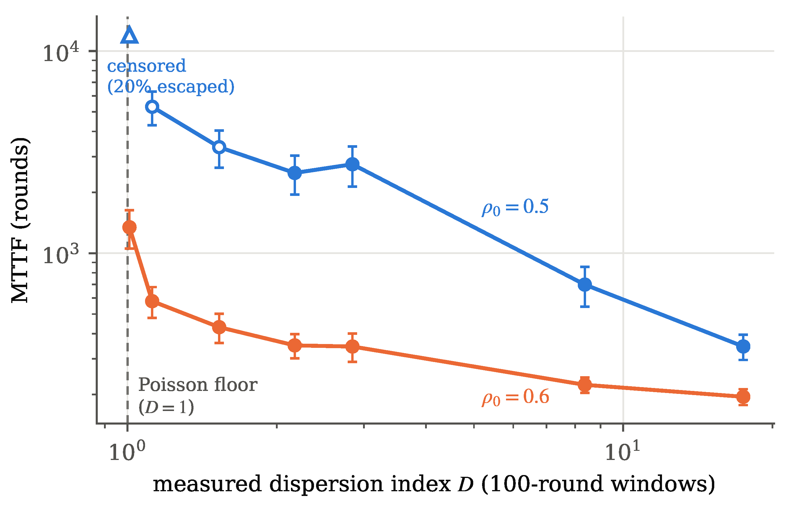
Figure 5.
Measured decode time of PyMatching 2 versus detection events per window (; each point the minimum of repeated calls). Growing the window in length at fixed density (blue) fits in this pass; packing the same window denser (orange) fits . Both are within the multi-pass bands quoted in the text. Green diamonds: the cluster axis, a fixed 40-round window at fixed background with k spatially clustered detector flips added, sitting well above both fits at the same event count. The shaded band marks the matched-event comparison: at identical E, density-packed windows cost and clustered windows length-grown ones.
Figure 5.
Measured decode time of PyMatching 2 versus detection events per window (; each point the minimum of repeated calls). Growing the window in length at fixed density (blue) fits in this pass; packing the same window denser (orange) fits . Both are within the multi-pass bands quoted in the text. Green diamonds: the cluster axis, a fixed 40-round window at fixed background with k spatially clustered detector flips added, sitting well above both fits at the same event count. The shaded band marks the matched-event comparison: at identical E, density-packed windows cost and clustered windows length-grown ones.
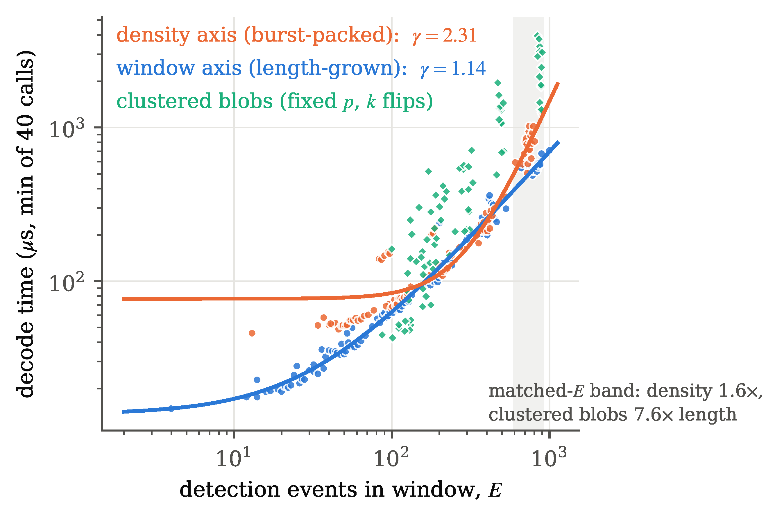
Figure 6.
Death round versus ramp slope under at fixed service calibration (, initial ; /arm, error bars ±sd). The deterministic system (diamonds) dies a constant ≈143 rounds after the drift-reversal clock (dotted), before the saddle-node (dashed). The stochastic ramp dies well before every clock, increasingly so for slow ramps, and at the two shallowest slopes it dies with no deterministic extinction inside the horizon at all. The constant-rate control at the ramp’s time-average dies sooner still: trajectory, not mean load, sets the failure epoch.
Figure 6.
Death round versus ramp slope under at fixed service calibration (, initial ; /arm, error bars ±sd). The deterministic system (diamonds) dies a constant ≈143 rounds after the drift-reversal clock (dotted), before the saddle-node (dashed). The stochastic ramp dies well before every clock, increasingly so for slow ramps, and at the two shallowest slopes it dies with no deterministic extinction inside the horizon at all. The constant-rate control at the ramp’s time-average dies sooner still: trajectory, not mean load, sets the failure epoch.
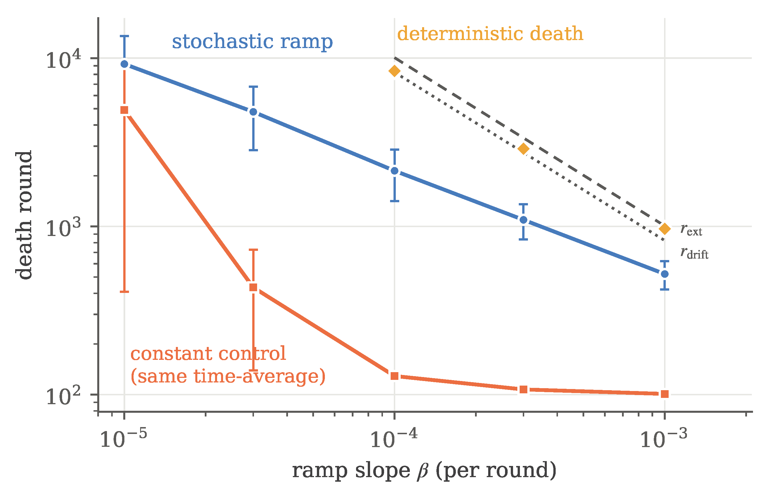

Table 1.
Deterministic basin boundary (first integer backlog outside the basin) from the drift-matched map (2), , , ; “∞” = globally stable.
Table 1.
Deterministic basin boundary (first integer backlog outside the basin) from the drift-matched map (2), , , ; “∞” = globally stable.
| ∞ | ∞ | ∞ | ∞ | ∞ | ∞ | |
| 658 | 148 | 44 | 25 | 15 | 6 | |
| 58 | 23 | 11 | 8 | 6 | 3 | |
| 9 | 6 | 4 | 3 | 3 | 2 | |
| 4 | 3 | 2 | 2 | 2 | 2 |
Table 2.
after a scheduled burst of the given excess detection events ( replications per cell, ). “D” marks cells where the drift-matched deterministic map (2) also diverges. Percentages carry the Wilson 95% intervals drawn in Figure 2; a 0/40 cell has a 95% upper bound of 8.8%.
| burst → | 0 | 25 | 50 | 100 | 200 | 400 | 800 |
|---|---|---|---|---|---|---|---|
| () | 0% | 0% | 0% | 0% | 0% | 0% | 0% |
| () | 0% | 0% | 0% | 0% | 8% | 100% D | 100% D |
| () | 0% | 0% | 43% | 100% D | 100% D | 100% D | 100% D |
| () | 100% | 100% | 100% D | 100% D | 100% D | 100% D | 100% D |
Table 3.
Spontaneous escape at , no perturbation (, horizon 12,000 rounds; threshold 100 outstanding rounds). MTTF ± values here and throughout are (≈95% CIs). The row is right-censored: 20% escaped within the horizon, so the data bound the median escape time, not the mean.
Table 3.
Spontaneous escape at , no perturbation (, horizon 12,000 rounds; threshold 100 outstanding rounds). MTTF ± values here and throughout are (≈95% CIs). The row is right-censored: 20% escaped within the horizon, so the data bound the median escape time, not the mean.
| MTTF (rounds) | ≈ wall clock | CV | ||
|---|---|---|---|---|
| 20% | median | ms | n/a | |
| 100% | ms | 0.83 | ||
| 100% | ms | 0.47 |
Table 4.
MTTF under square-wave modulated arrivals at fixed mean load (, no burst, /cell, horizon 12,000 rounds), sorted by measured dispersion D. Parenthesised entries are right-censored cells (conditional mean of the escaped replications, biased low).
Table 4.
MTTF under square-wave modulated arrivals at fixed mean load (, no burst, /cell, horizon 12,000 rounds), sorted by measured dispersion D. Parenthesised entries are right-censored cells (conditional mean of the escaped replications, biased low).
| arm (a, ) | meas. D | : | MTTF | : MTTF | CV |
|---|---|---|---|---|---|
| base | 1.01 | 20% | median | 0.83 | |
| , 20 | 1.12 | 67% | () | 0.67 | |
| , 20 | 1.53 | 93% | () | 0.64 | |
| , 20 | 2.17 | 100% | 0.53 | ||
| , 80 | 2.84 | 100% | 0.62 | ||
| , 80 | 8.36 | 100% | 0.34 | ||
| , 80 | 17.5 | 100% | 0.35 |
Table 5.
Bounded-window mitigation at under a 200-event burst (, horizon 6,000 rounds). The column is the closed-form drift-matched per-round cost; the budget is 10. The classifier is >100 rounds outstanding at the horizon; for this flags slow recovery, not instability (see text).
Table 5.
Bounded-window mitigation at under a 200-event burst (, horizon 6,000 rounds). The column is the closed-form drift-matched per-round cost; the budget is 10. The classifier is >100 rounds outstanding at the horizon; for this flags slow recovery, not instability (see text).
| window | at horizon) | mean backlog (rounds) | busy | |
|---|---|---|---|---|
| 0% | 4.0 | 87% | 7.9 | |
| 0% | 3.3 | 85% | 6.3 | |
| 0% | 5.3 | 86% | 6.3 | |
| 0% | 13.3 | 87% | 7.5 | |
| 90% | 215 | 98% | 9.9 | |
| 100% | 863 | 98% | 13.7 | |
| greedy | 100% | 2,190 | 98% | (basin) |
Table 6.
Bounded buffers under the 200-event burst (, , drop-newest, ; ± is SE). Saturation = outstanding work pinned at or above C for the final 1,000 arrival rounds. is the drift-matched per-round cost of the cap’s implicit window under greedy; for the policy at every cap.
Table 6.
Bounded buffers under the 200-event burst (, , drop-newest, ; ± is SE). Saturation = outstanding work pinned at or above C for the final 1,000 arrival rounds. is the drift-matched per-round cost of the cap’s implicit window under greedy; for the policy at every cap.
| cap C | greedy: dropped / | : dropped / | |||
|---|---|---|---|---|---|
| 8 | 0% | 0% | 7.5 | ||
| 16 | 0% | 0% | 9.9 | ||
| 32 | 18% | 0% | 13.6 | ||
| 64 | 100% | 0% | 19.1 | ||
| 128 | 100% | 0% | 26.9 | ||
Table 7.
Basin boundary (rounds) at the measured exponents, drift-matched map.
| window axis, (pass 1) | 38,331 | 3,211 | 423 | 75 |
| window axis, (pass 2) | 79 | 30 | 13 | 7 |
| window axis, (band edge) | 20 | 11 | 6 | 4 |
| density axis, | 4 | 3 | 2 | 2 |
Table 8.
The three axes across decoder implementations (; same stratified min-of-reps timing; matched-E ratios at 600–900 events, measured adjacently, relative to each decoder’s own length-grown windows). The union-find exponent fits are quoted for completeness but are not credible (/: decode time at fixed E varies by orders of magnitude); its matched-E ratios are the meaningful entries.
Table 8.
The three axes across decoder implementations (; same stratified min-of-reps timing; matched-E ratios at 600–900 events, measured adjacently, relative to each decoder’s own length-grown windows). The union-find exponent fits are quoted for completeness but are not credible (/: decode time at fixed E varies by orders of magnitude); its matched-E ratios are the meaningful entries.
| decoder | window (5%-SSE band) | density | density | cluster |
|---|---|---|---|---|
| PyMatching 2 (this pass) | 1.15 [0.97, 1.35] | 2.14 [1.76, 2.60] | ||
| fusion-blossom | 1.49 [1.41, 1.58] | 2.20 [1.95, 2.48] | ||
| ldpc union-find | (1.18 [0.5, 2.7]) | (2.33 [1.2, 3.5]) | ||
| BP+OSD | 0.97 [0.89, 1.06] | 0.50 [0.50, 0.66] |
Disclaimer/Publisher’s Note: The statements, opinions and data contained in all publications are solely those of the individual author(s) and contributor(s) and not of MDPI and/or the editor(s). MDPI and/or the editor(s) disclaim responsibility for any injury to people or property resulting from any ideas, methods, instructions or products referred to in the content. |
© 2026 by the authors. Licensee MDPI, Basel, Switzerland. This article is an open access article distributed under the terms and conditions of the Creative Commons Attribution (CC BY) license (http://creativecommons.org/licenses/by/4.0/).
Copyright: This open access article is published under a Creative Commons CC BY 4.0 license, which permit the free download, distribution, and reuse, provided that the author and preprint are cited in any reuse.