

Submitted:
17 August 2026
Posted:
18 August 2026
You are already at the latest version
Abstract
The suspended matter concentration (TSM) and Secchi disk depth (SDD) are key parameters describing seawater quality, directly reflecting the turbidity of seawater and the degree of light absorption and scattering by seawater. In this study, based on GOCI data, three different atmospheric correction (AC) algorithms were employed to retrieve the TSM and SDD of the Yellow Sea and Bohai Sea, and conducted with in-situ data. Leveraging the high observation frequency of GOCI, differences in the hourly variation characteristics of TSM and SDD under different AC algorithms were further analyzed. The results show that at the same pixel, the values of TSM and SDD retrieved using different atmospheric correction algorithms exhibit non-negligible differences. In some sea areas, there are obvious anomalies in the coupled response of TSM and SDD obtained using the same atmospheric correction algorithm. Most critically, the hourly trends of TSM and SDD obtained by different AC algorithms may diverge or even be completely opposite, especially in highly turbidities waters. This suggests that AC algorithmic selection is not just a preprocessing detail, but a factor that can radically alter the interpretation of short-term biogeochemical dynamics. The findings suggest an important methodological warning for high-frequency time-series research in ocean color remote sensing.
Keywords:
suspended matter concentration
; transparency
; GOCI
; Chinese coastal seas
1. Introduction
The total suspended matter (TSM) and Secchi disk depth (SDD) are core parameters revealing the state of aquatic ecosystems and changes in water quality [1]. suspended matters serve as the carrier of photoactive substances, and their concentration directly regulates the light attenuation characteristics, primary productivity levels, and pollutant migration and transformation processes in water bodies, exerting a decisive influence on the estimation of carbon cycle flux and habitat quality of aquatic organisms [2]. Meanwhile, as a comprehensive reflection of the optical properties of water, transparency not only intuitively indicates the cumulative effects of suspended particles and dissolved colored substances, but also serves as a key indicator for assessing eutrophication levels, habitat suitability of benthic vegetation, and the aesthetic value of water [3]. However, driven by both hydro-meteorological conditions and human activities, these parameters exhibit high variability in the temporal and spatial dimensions, posing severe challenges to accurate monitoring. Although traditional ship-based point sampling observation methods can provide high-precision in-situ data, they are not effective for large-scale, high-frequency dynamic monitoring of water quality because of their limited spatial representativeness, low temporal resolution, and uneconomic cost [4,5]. Particularly in optically complex waters such as estuarine and coastal zones and large inland lakes, complete concentration gradients and transport processes often cannot be captured through discrete sampling because of the drastic spatiotemporal variability of suspended matters. Moreover, in conventional monitoring networks, the deployment density is constrained by human and material resources, with insufficient response capabilities for remote waters or emergency events [6]. These inherent limitations highlight the urgency of developing alternative monitoring technologies. Remote sensing technology has emerged as an irreplaceable technical means for TSM and SDD retrieval as it can be used to capture the spectral response characteristics of water color elements, facilitating the transition from local point measurements to regional surface observations [7,8]. After decades of development, this field has seen major progresses through single-band empirical statistical models, semi-analytical algorithms based on radiative transfer theory, and in recent years, deep integration of machine learning and deep learning techniques, which have significantly improved retrieval accuracy and robustness in optically complex waters [9]. In particular, the proliferation of multispectral satellites and UAV hyperspectral platforms, combined with the optimization of atmospheric correction models, has enabled water quality parameter mapping at high spatiotemporal resolution [10,11]. However, existing algorithms still face numerous challenges in terms of regional adaptability, physical interpretability, and atmospheric correction accuracy [12,13].
Regarding the retrieval of suspended matter concentration, empirical statistical models have been widely applied because of their computational simplicity; based on the statistical correlation between remote-sensing reflectance and TSM, these models construct regression equations through single-band, band ratio, or multi-band combinations [5,14]. Semi-analytical algorithms parse the explicit relationship between remote-sensing reflectance and inherent optical properties (IOPs) through radiative transfer equations, and then utilize the bio-optical association between particle backscattering coefficients and TSM to achieve physical inversion [15,16]. Machine learning methods can capture high-dimensional nonlinear relationships between spectral features and TSM through non-parametric modeling, and multiple case studies have demonstrated the superior accuracy and robustness of ensemble learning algorithms such as random forest, support vector machine, and extreme gradient boosting compared to traditional regression [2,6,7,17]. Regarding water transparency, empirical statistical models based on blue-green band ratios, semi-analytical algorithms incorporating bio-optical models, and physical analytical methods have been developed to estimate transparency by retrieving IOPs [18]. After improvement, the quasi-analytical algorithm (QAA) framework proposed by Lee et al. [19], can be used for transparency estimation, in which total absorption and backscattering coefficients are retrieved from remote-sensing reflectance, and inversion is then achieved by combining the theoretical relationship between the Secchi depth and these IOPs. The framework has been validated using 338 globally measured Rrs and Zsd in-situ datasets, and extended to Landsat 8 and other satellite remote sensing observation data. A semi-analytical algorithm was developed for MERIS data, incorporating optical type classification of water and customized model parameters, and it has significantly reduced estimation errors in complex waters [20,21,22]. However, among numerous studies, only few scholars have discussed the impact of different atmospheric correction algorithms on the retrieval accuracy of suspended matter concentration and transparency. The ratio of water-leaving radiance to downward irradiance immediately above the water surface is defined as the remote-sensing reflectance (Rrs) of the water body spectra, which cannot be directly measured. However, high-precision ocean remote sensing studies (e.g., suspended matter concentration and transparency retrieval) require precise Rrs data [23,24]. The water-leaving radiance contributed by the water body accounts for less than 10% of the total signal received by ocean color satellite sensors; therefore, atmospheric correction is required for the received signal, which is also one of the key processes in ocean optical remote sensing. Accurate atmospheric correction is a prerequisite for obtaining high-precision Rrs data and achieving high-precision retrieval of water color information [19]. Currently, atmospheric correction algorithms for optically complex waters in coastal areas include the bright pixel method, dark pixel method, neural network method, spectral matching method, MUMM method, spectral optimization method, etc. Another research topic requiring attention in ocean optical remote sensing is the error analysis of water color information retrieved by applying different atmospheric correction algorithms to the same sensor [24,25,26,27].
Over the past decades, several countries around the world have launched various spaceborne ocean color sensors for daily global ocean observation. The main observation platforms are polar-orbiting satellites, such as the Sea-viewing Wide Field-of-view Sensor (SeaWiFS), Moderate Resolution Imaging Spectroradiometer (MODIS), Medium Resolution Imaging Spectrometer (MERIS), Visible Infrared Imaging Radiometer Suite (VIIRS), and Ocean and Land Colour Instrument (OLCI). The historically significant Geostationary Ocean Color Imager (GOCI) also remains widely used. With its high-frequency observation capability, GOCI enables the analysis of hourly variations in marine biogeochemical information.
This study analyzed differences in the accuracy of different operational atmospheric correction algorithms for retrieving suspended matter concentration and transparency using GOCI data of the Yellow Sea and Bohai Sea. Differences in hourly variation results for suspended matter concentration and transparency among different atmospheric correction algorithms were analyzed. To this end, the Case-2 suspended matter concentration retrieval model and the semi-analytical transparency retrieval model by Lee (2015) were adopted. The results indicate that the selection of atmospheric correction algorithm can affect the analysis results of intra-day hourly variation patterns, and the variation trends obtained using different atmospheric correction algorithms may even reverse. These findings provide important methodological warnings for high-frequency time-series research in ocean color remote sensing
2. Data and Methods
2.1 Data
2.1.1 In-Situ Data
This study utilized in-situ measured data from three cruises in 2014, 2018, and 2019, covering the Yellow Sea and Bohai Sea (Figure 1). The measured parameters included total suspended matter (determined using the gravimetric method) and transparency (measured using the Secchi disk method).
2.1.2 GOCI Data
GOCI is the primary sensor aboard COMS (Communication Ocean and Meteorological Satellite). COMS was launched in 2010 as the world's first geostationary ocean color satellite. It covers the Bohai Sea, Yellow Sea, and parts of the East China Sea, acquiring 8 scenes per day from 8:00 AM to 3:00 PM local time, with one image per hour. The swath width of GOCI is 2500×2500 km, with a spatial resolution of 500 m and spectral bands ranging from 0.412 to 0.865 μm (6 visible bands and 2 near-infrared bands). Unlike traditional polar-orbiting ocean color satellites, GOCI enables the observation of diurnal variations in biogeochemical parameters, thus facilitating the monitoring of hourly changes in coastal water quality, red tides, green tides, and other phenomena. The GOCI L1B data used in this study were temporally consistent with the in-situ experimental data.
2.2 Atmospheric Correction (AC) Algorithms
2.2.1 AC Algorithms of KOSC GDPS
The official website of the Korea Ocean Satellite Center (KOSC) currently provides global users with six versions of the installation program known as the GOCI Data Processing System (GDPS) for free: GDPS1.1, GDPS1.2, GDPS1.3, GDPS1.4, GDPS1.4.1, and GDPS2.0. In GDPS2.0, atmospheric correction is performed using the spectral relationships in the aerosol multiple-scattering reflectance (SRAMS) among different wavelengths to directly calculate the contribution of near-infrared multiple-scattering reflectance [28]. In this study, corrected reflectance spectral (Rrs(λ)) data were obtained from the GOCI L1B data using the default atmospheric correction algorithms of GDPS2.0.
2.2.2 AC Algorithms of SeaDAS
SeaDAS provides a variety of atmospheric correction algorithms. In this study, atmospheric correction of GOCI data was conducted using the default atmospheric correction algorithm of SeaDAS 8.2 [29,30] (i.e., NASA standard atmospheric correction algorithm, denoted as Seadas-Default in this paper) and MUMM atmospheric correction algorithm [31] (denoted as Seadas-MUMM in this paper). In this manner, the corrected remote sensing reflectance spectral (Rrs(λ)) data were obtained.
2.3 Retrieval Algorithm of TSM
Based on GOCI multispectral band ratios, GDPS is equipped with an inversion algorithm suitable for the concentration of suspended solids in Class II water bodies. The method is applicable to highly turbid coastal and inland waters.
where Rrs745, Rrs680, Rrs555, and Rrs490 represent the atmospherically corrected remote-sensing reflectance data at 745 nm, 680 nm, 555 nm, and 490 nm bands, respectively.
2.4 Retrieval Algorithm of SDD
Lee et al. proposed a new theoretical model for retrieving water transparency and validated this model using 338 globally measured Rrs(λ) and Zsd in-situ datasets (covering oceanic, coastal, and inland waters, with approximately 200 matched data over the China Seas) [32]. This model algorithm exhibited high universality for any water type. Later, it was extended and applied to MODIS, Landsat, GOCI, and other satellite data for retrieving seawater transparency values [33,34]. The model formula is as follows.
where , is the remote-sensing reflectance at the wavelength corresponding to the Kd (λ) minimum value.
2.4 Accuracy Evaluation Index
In this study, the comprehensive quantitative evaluation was performed for retrieval accuracy in terms of correlation coefficient (r), mean relative error (ε), root mean square error (RMSE), and mean bias (Bias). Oi represents the measured data, Si represents the retrieved data from GOCI.
3. Results
3.1. Accuracy Comparison of TSM and SDD Retrieval
To quantitatively evaluate the applicability of different atmospheric correction algorithms for the remote sensing retrieval of water color parameters in the Yellow Sea and Bohai Sea, the following three atmospheric correction methods were employed: GDPS2.0, Seadas_Default, and Seadas_MUMM. The retrieved values were then validated with in-situ measured data. Comprehensive quantitative evaluation was performed for retrieval accuracy in terms of correlation coefficient (r), mean relative error (ε), root mean square error (RMSE), and mean bias (Bias), and the results are shown in Figure 2 and Figure 3. Regarding TSM (Figure 2), the GDPS2.0 algorithm showed a correlation coefficient of r = 0.91 with measured data, indicating strong linear correlation, but the retrieval results exhibited significant systematic overestimation, with Bias = 1.308 mg/L, mean relative error ε = 40%, RMSE = 0.48 mg/L, and data points generally distributed above the 1:1 reference line; the Seadas_Default algorithm achieved the same correlation coefficient of r = 0.91, with the optimal comprehensive retrieval accuracy, ε of only 22%, RMSE = 0.26 mg/L, Bias of only 0.08, and scatter points uniformly and symmetrically distributed along the 1:1 reference line without any obvious offset; the Seadas_MUMM algorithm showed the lowest correlation (r = 0.82), with the most prominent overestimation phenomenon, Bias = 1.57 mg/L, ε = 42%, RMSE = 0.57 mg/L, and the largest data dispersion, exhibiting the worst TSM retrieval performance. In contrast, for SDD (Figure 3), the GDPS2.0 algorithm exhibited optimal retrieval performance, with a correlation coefficient as high as r = 0.94, mean relative error as low as 18.9%, RMSE = 0.26 m, Bias approaching 0, and scatter points highly concentrated along the 1:1 reference line with almost no systematic bias; the Seadas_MUMM algorithm ranked second in accuracy, with r = 0.90, ε = 22%, RMSE = 0.30 m, and only a small systematic overestimation (Bias = 0.64 m); the Seadas_Default algorithm maintained high correlation (r=0.93), but the error and overestimation issues were significantly aggravated, with ε rising to 32%, RMSE = 0.39 m, and Bias reaching 1.10 m. Overall, Seadas_Default showed the highest overall retrieval deviation among the three. The comparison of TSM and SDD results shows that there is no optimal atmospheric correction scheme universally applicable to all water color parameters. Therefore, it is necessary to conduct preliminary comparative analyses and targeted optimization of atmospheric correction algorithms according to the target retrieval parameters, rather than directly applying a single default correction product. In this manner, errors and trend deviations introduced by preprocessing can be minimized, thus ensuring the reliability and scientific validity of relevant conclusions.
3.2 Spatial Distribution of TSM and SDD from Different AC Algorithms
Based on GOCI imagery results from 05:16 UTC (13:16 local time) on March 9, 2018, this study compared the spatial distribution characteristics of suspended matter concentration and transparency derived from the three atmospheric correction algorithms (GDPS2.0, NASA standard algorithm, MUMM algorithm). As shown in Figure 4 and Figure 5, the retrieval results from the three atmospheric correction algorithms could effectively characterize the basic spatial gradient from nearshore to offshore, but significant differences appear in quantitative values and detailed representation of the nearshore. Particularly in the areas marked by circles in the figures, the spatial distributions show significant differences in both numerical magnitude and data coverage among the three algorithms.
Using the official GDPS2.0 retrieval results as the baseline reference, the variation rates of results from the NASA standard algorithm and MUMM were further quantitatively calculated, as shown in Figure 6 and Figure 7. For suspended matter concentration (Figure 6), the NASA standard algorithm showed an overall significant underestimation in the coastal waters of the northern Yellow Sea and around the Shandong Peninsula, with relative biases generally ranging from -50% to -100%; a certain degree of overestimation was found over small local areas, with maximum deviations reaching approximately 1-fold. The spatial distribution of TSM from the MUMM algorithm was similar to that from the NASA standard algorithm, but the area of overestimation with deviation magnitude reaching approximately 1-fold was significantly larger, particularly in the Yellow Sea-Bohai Sea confluence region, where TSM retrieval results were overall higher than that from GDPS2.0 by 50% to 100%. For water transparency (Figure 7), the magnitude of parameter deviation associated with different atmospheric correction algorithms was much compared with TSM. The NASA standard correction algorithm showed severe overestimation of water transparency compared to the GDPS2.0 algorithm in most open sea areas, with relative increases exceeding 150% in local regions. Moreover, it showed significant underestimation in the high-turbidity coastal waters of the southern Yellow Sea, with negative deviations reaching -50% to -100%. Relative to GDPS2.0, spatial differences in the bias of SDD from the MUMM algorithm were even more pronounced, with the overestimation of transparency exceeding 100% in large areas of the southern Yellow Sea, but significant underestimation still existed in the coastal areas of the northern Yellow Sea. Overall, different atmospheric correction methods introduced biases with extremely strong spatial variability in the retrieval of color parameters in Case-2 waters.
Statistical analysis was conducted on the spatial distribution and occurrence frequency of times at which extreme values of suspended matter concentration and transparency (retrieved from GOCI data over the Yellow Sea and Bohai Sea on March 9, 2018) were observed (Figure 8, Figure 9 and Figure 10). The results show an inverse coupling pattern between the times of extreme TSM and SDD values. Maximum TSM and minimum SDD values are concentrated at 08:16 (local time) in the early morning, whereas minimum TSM and maximum SDD values are mostly concentrated at 13:16-15:16 (local time) in the afternoon, reflecting the diurnal variation process of water body resuspension in the morning and particle settling in the afternoon. However, the concentration degrees of the frequency of extreme TSM and SDD values under the three different atmospheric correction algorithms significantly differed: GDPS2.0 showed prominent extreme value peaks and optimal temporal aggregation; SeaDas MUMM ranked the second, and SeaDas Default exhibited the most dispersed frequency distribution. These results all indicate that the application of different atmospheric correction algorithms for intra-day variation analysis of different water quality parameters will lead to inconsistent conclusions. Therefore, researchers should carefully consider the choice of atmospheric correction algorithm when conducting hourly variation analysis.
3.3 Coupling Responses of TSM and SDD with Different AC algorithms
The fundamental reason for the differences in the results from different atmospheric correction algorithms lies in the different separation mechanisms of each algorithm for aerosol scattering and water-leaving radiance. Owing to these differences in model principles, the three algorithms feature different correction effects for different turbidity regions and at different times, ultimately affecting the retrieval of water color parameters.
To reveal the impact of different atmospheric correction algorithms on the retrieval of the spatial gradient of water color parameters, this study compared the zonal spatial variation characteristics of water transparency (SDD) and total suspended matter (TSM) retrieved using GDPS2.0, Seadas_Default, and Seadas_MUMM. For this purpose, GOCI satellite observation data at 05:16 (UTC) on March 9, 2018, along the 124°E longitudinal transect (blue line in Figure 11) was employed. The spatial variation of transparency along the longitudinal transect (124°E) is shown in Figure 12 (a). The NASA standard algorithm and MUMM algorithm provided essentially matching results, whereas the GDPS2.0 algorithm provided significantly different results, and this difference was reflected not only in the numerical values but also in the trend changes. The same difference was observed for the variation of suspended matter concentration as well (Figure 12 (b)). Research shows that there is a strong coupling response between suspended solids concentration and transparency. In sea areas with high transparency, the concentration of suspended solids is relatively low, while in sea areas with low transparency, the concentration of suspended solids is relatively high [35]. The change diagram in Figure 12 shows that the transparency data retrieved based on GDPS2.0 (Figure 12 (a) red curve) and the suspended solids concentration data retrieved based on Seadas_Default (Figure 12 (b) blue curve) show this strong coupling effect along the latitude direction. On the contrary, the transparency and suspended matter concentration data obtained based on the same atmospheric correction algorithm do not show this coupling response.
4. Discussion
The divergent retrieval performances among the three atmospheric correction algorithms can be attributed to their distinct theoretical foundations in separating aerosol scattering and water-leaving radiance[28,29,30]. Critically, our results demonstrate that algorithm performance cannot be generalized across parameters: the same atmospheric correction scheme may yield optimal results for one water quality indicator while producing substantial biases for another, implying that different retrieval models propagate band-specific atmospheric residuals differently. And inconsistent coupling responses between TSM and SDD were observed even when using the same atmospheric correction algorithm, challenging the assumption that algorithm choice uniformly affects all water quality parameters.
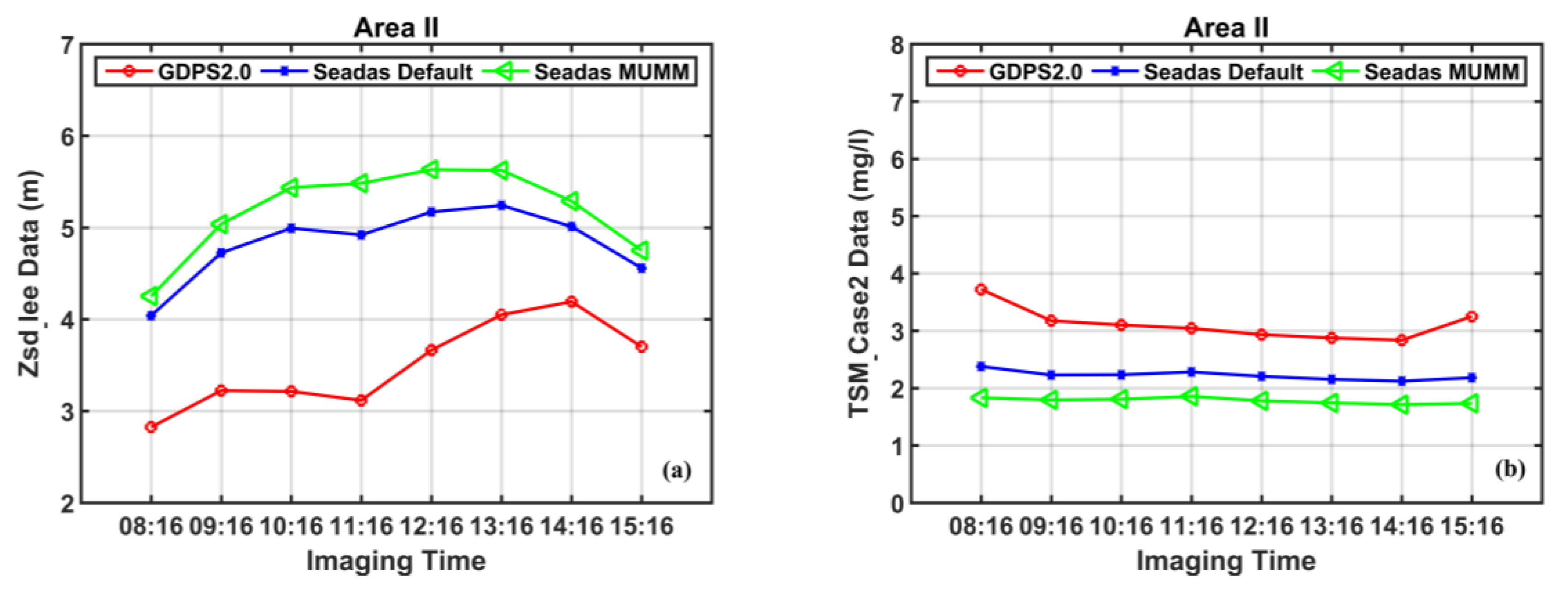
Then, does the choice of different atmospheric correction algorithms produce inconsistent results for the conclusions of SDD and TSM changes in different regions at different times? To investigate this, 8 hours temporal dynamic variation patterns of water transparency and total suspended matter were retrieved using the three atmospheric correction schemes (GDPS2.0, Seadas_Default, and Seadas_MUMM) based on GOCI hourly remote sensing observation data from 08:16 to 15:16 (local time) on March 9, 2018, for Sea Area Ⅰ and Sea Area Ⅱ ( red areas in Figure 11). The results are shown in Figure 13 and Figure 14, respectively. During the early hours of the observation period (08:16-14:16), the overall temporal variation patterns of the retrieval parameters from the three algorithms were essentially consistent, with transparency showing an overall upward trend and suspended matter concentration showing negatively correlated changes in fluctuation. At the same time, stable numerical differences were observed among the algorithms, with GDPS2.0 generally providing lower transparency and higher suspended matter concentration, where as Seadas_Default and Seadas_MUMM provided similar values. However, during later hours (14:16-15:16), the hourly variation trends of retrieved parameters from different algorithms showed distinct differences. For high turbidity Sea Area I, the transparency data has been low, and the concentration of suspended matter retrieved by GDPS2.0 has increased rapidly. In contrast, with the other two algorithms, transparency recovered and suspended matter concentration decreased, showing completely opposite parameter variation trends compared with GDPS2.0. This phenomenon was also observed in Sea Area Ⅱ, with suspended matter concentration from GDPS2.0 showing significant increase during this period; in contrast, suspended matter concentration from the other two algorithms maintained a steady small fluctuations. As observed, different atmospheric correction algorithms not only cause numerical deviations in retrieval results, but also lead to differences in the hourly variation patterns of biogeochemical parameters, even leading to completely opposite evolution characteristics.
Research shows that AC algorithm selection can fundamentally alter the interpretation of hourly variation patterns, with trends becoming completely opposite during intra-day transition periods (14:16–15:16). During these late-afternoon hours, declining solar elevation angles modify atmospheric path length and scattering geometry, and the three algorithms respond to these changing illumination conditions differently: GDPS2.0's spectral extrapolation becomes less reliable, the NASA standard's dark pixel selection is increasingly compromised, and MUMM's multiple scattering corrections may overcompensate for increased path radiance. This geometrically induced bias structure creates a time-dependent artifact that can be mistaken for genuine biogeochemical signals. These findings carry a clear methodological warning: atmospheric correction is not a neutral preprocessing step but a decision that shapes scientific conclusions, and studies attributing diurnal patterns solely to physical or biological processes risk confounding algorithmic artifacts with environmental signals. When we conduct hourly variation analysis studies using GOCI data, we need to be cautious about the results in the late afternoon.
But several limitations should be acknowledged during this study. The in-situ validation dataset, though spanning three years, is limited to the stations with sparse coverage in the central Yellow Sea and eastern Bohai Sea, and the hourly variation analysis is confined to a single date (March 9, 2018), which may not capture seasonal variability in algorithm performance. Nevertheless, the three algorithms evaluated represent the most widely used operational approaches for GOCI data processing, ensuring the direct relevance of our findings to current practice. Looking ahead, as next-generation geostationary ocean color sensors deliver increasingly higher temporal resolution data, we recommend that researchers adopt multi-algorithm ensemble approaches, maintain consistent atmospheric correction schemes throughout time-series analyses.
5. Conclusions
The results of this study suggest that the regional adaptability of atmospheric correction algorithms should be fully considered when conducting research on variations in biogeochemical parameters of water, because non-negligible quantitative discrepancies exist among retrieval results from different atmospheric correction algorithms at the same pixel, with relative biases reaching −100% to +200% in certain coastal regions. Most critically, the hourly trends of TSM and SDD obtained by different AC algorithms may diverge or even be completely opposite, especially in highly turbidities waters. This suggests that algorithmic selection is not just a preprocessing detail, but a factor that can radically alter the interpretation of short-term biogeochemical dynamics. When we conduct hourly variation analysis studies using GOCI data, we need to be cautious about the results in the late afternoon. This study can provide methodological references for high-frequency time-series research in ocean color remote sensing over coastal sea areas, and also provide theoretical support for data preprocessing in studies involving intra-day variation of similar biogeochemical parameters.
Author Contributions
Conceptualization: J.C. and W.Y.; methodology: J.C. and X.L.; software: J.C. and X.L.; validation: C.X. and S.C..; investigation: J.C. and X.L.; data curation: Z.L. and S.C.; writing—original draft preparation: J.C. and X.L.; writing—reviewand editing: W.Y. and X.L.; visualization: L.W. and X.Z.; project administration: W.Y.; fundingacquisition: W.Y., S.C., L.W., C.X., Z.L. and X.Z. All authors have read and agreed to the published version of the manuscript.
Funding
This research is supported by the following research projects: Program of Opening Ceremony to Select the Best Candidates of the Key Laboratory of Marine Ecological Monitoring and Restoration Technologies, MNR (Grant No. MEMRT2024JBGS01); China Three Gorges Investment Management Co., Ltd. (Grant No. CTGIM-2025-ZC001); Huaneng(Shanghai) Clean Energy Development CO., Ltd.; Shanghai Electric Power CO., Ltd.; Shanghai Electric Wind Power Group Co., Ltd.; CRCC Harbour & Channel Engineering Bureau Group CO., Ltd..
Data Availability Statement
Publicly available datasets were analyzed in this study.
Acknowledgments
The authors would like to thank the observation and Research Station of Huaniaoshan East China Sea Ocean-Atmosphere Integrated Ecosystem, Ministry of Natural Resources for providing In-situ data free of charge.
Conflicts of Interest
The authors declare no conflicts of interest.
References
- Wu, Z.; Pang, J.; Li, J.; Wang, Y.; Ruan, J.; Zhang, X.; Yang, L.; Pang, Y.; Gao, Y. A review of remote sensing-based water quality monitoring in turbid coastal waters. Intell. Mar. Technol. Syst. 2025, 3. [Google Scholar] [CrossRef]
- Song, G.; Jiang, Y.; Lei, X.; Zhai, S. Measurement of suspended sediment concentration at the outlet of the yellow river canyon: Using sentinel-2 images and machine learning. Remote Sens. 2025, 17, 2424. [Google Scholar] [CrossRef]
- Bai, S.; Gao, J.; Sun, D.; Tian, M. Monitoring water transparency in shallow and eutrophic lake waters based on GOCI observations. Remote Sens. 2020, 12, 163. [Google Scholar] [CrossRef]
- Cao, Q.; Yu, G.; Qiao, Z. Application and recent progress of inland water monitoring using remote sensing techniques. Environ. Monit. Assess. 2022, 195. [Google Scholar] [CrossRef] [PubMed]
- Topliss, B.J.; Almos, C.L.; Hill, P.R. Algorithms for remote sensing of high concentration, inorganic suspended sediment. Int. J. Remote Sens. 1990, 11, 947–966. [Google Scholar] [CrossRef]
- Ding, C.; Zhang, X.; Ma, S.; Han, W.; Lu, Y.; Yin, J. Estuary water quality classification through deep learning image segmentation, an example of hangzhou bay. In Proceedings of the 2021 9th International Conference on Agro-Geoinformatics (Agro-Geoinformatics), 2021. [Google Scholar] [CrossRef]
- Zaghian, S.; Mohammadzadeh, A.; Ghorbanian, A.; Bovolo, F.; Niroumand-Jadidi, M. Enhancing suspended sediment concentration retrieval by integrating thermal infrared and optical bands of landsat-8 and machine learning algorithms. Int. J. Remote Sens. 2023, 44, 5814–5844. [Google Scholar] [CrossRef]
- Kwon, S.; Shin, J.; Seo, I.W.; Noh, H.; Jung, S.H.; You, H. Measurement of suspended sediment concentration in open channel flows based on hyperspectral imagery from UAVs. Adv. Water Resour. 2022, 159. [Google Scholar] [CrossRef]
- Xie, R.; Zhou, Z.; Kong, J.; Wang, C.; Wang, Y.; Li, L.; Ding, C.; Li, R.; Zhang, X. Multi-algorithm comparison for water quality retrieval: Integrating landsat-8 OLI and machine learning in karst plateau reservoirs. Water 2025, 17, 1781. [Google Scholar] [CrossRef]
- Pan, H.; Lyu, H.; Wang, Y.; Jin, Q.; Wang, Q.; Li, Y.; Fu, Q. An improved approach to retrieve IOPs based on a quasi-analytical algorithm (QAA) for turbid eutrophic inland water. IEEE J. Sel. Top. Appl. Earth Obs. Remote Sens. 2015, 8, 5177–5189. [Google Scholar] [CrossRef]
- Yang, W.; Matsushita, B.; Chen, J.; Yoshimura, K.; Fukushima, T. Retrieval of inherent optical properties for turbid inland waters from remote-sensing reflectance. IEEE Trans. Geosci. Remote Sens. 2013, 51, 3761–3773. [Google Scholar] [CrossRef]
- Bi, S.; Hieronymi, M.; Röttgers, R. Bio-geo-optical modelling of natural waters. Front. Mar. Sci. 2023, 10, 1196352. [Google Scholar] [CrossRef]
- Morel, A.; Maritorena, S. Bio-optical properties of oceanic waters: A reappraisal. J. Geophys. Res. Ocean. 2001, 106, 7163–7180. [Google Scholar] [CrossRef]
- Onderka, M.; Rodný, M. Can suspended sediment concentrations be estimated from multispectral imagery using only image-derived information? J. Indian Soc. Remote Sens. 2010, 38, 85–97. [Google Scholar] [CrossRef]
- Pitarch, J.; Bellacicco, M.; Organelli, E.; Volpe, G.; Colella, S.; Vellucci, V.; Marullo, S. Retrieval of particulate backscattering using field and satellite radiometry: Assessment of the QAA algorithm. Remote Sens. 2020, 12, 77. [Google Scholar] [CrossRef]
- Joshi, I.D.; D'Sa, E.J. An estuarine-tuned quasi-analytical algorithm (QAA-v): Assessment and application to satellite estimates of SPM in galveston bay following hurricane harvey. Biogeosciences 2018, 15, 4065–4086. [Google Scholar] [CrossRef]
- Gupta, N.; Valarmathi, B.; Hiwanj, I. A comparison of deep learning and machine learning methods for water quality prediction. In Proceedings of the 2025 3rd International Conference on Intelligent Data Communication Technologies and Internet of Things (IDCIoT) 2025, 1361–1368. [Google Scholar] [CrossRef]
- Liu, X.; Meng, X.; Wang, X.; Bi, D.; Chen, L.; Lou, Q. Using a semi-analytical model to retrieve secchi depth in coastal and estuarine waters. Acta Oceanol. Sin. 2020, 39, 103–112. [Google Scholar] [CrossRef]
- Lee, Z.; Arnone, R.; Hu, C.; Werdell, P.J.; Lubac, B. Uncertainties of optical parameters and their propagations in an analytical ocean color inversion algorithm. Appl. Opt. 2010, 49, 369. [Google Scholar] [CrossRef] [PubMed]
- Msusa, A.D.; Jiang, D.; Matsushita, B. A semianalytical algorithm for estimating water transparency in different optical water types from MERIS data. Remote Sens. 2022, 14, 868. [Google Scholar] [CrossRef]
- Kulshreshtha, A.; Shanmugam, P. Estimation of underwater visibility in coastal and inland waters using remote sensing data. Environ. Monit. Assess. 2017, 189. [Google Scholar] [CrossRef] [PubMed]
- Alikas, K.; Kratzer, S. Improved retrieval of secchi depth for optically-complex waters using remote sensing data. Ecol. Indic. 2017, 77, 218–227. [Google Scholar] [CrossRef]
- Nguyen, H.C.; Jung, J.; Lee, J.; Choi, S.U.; Hong, S.Y.; Heo, J. Optimal atmospheric correction for above-ground forest biomass estimation with the ETM+ remote sensor. Sensors 2015, 15, 18865. [Google Scholar] [CrossRef] [PubMed]
- Zhang, Y.; Wang, X.; Chen, Y. An improved 6S code for atmospheric correction based on water vapor content. Adv. Remote Sens. 2012, 1, 14–18. [Google Scholar] [CrossRef]
- Yu, W.; Wen, Y.; Wang, R. Water pollution environment information extraction based on landsat images. Proceedings of SPIE, International Conference on Geographic Information and Remote Sensing Technology (GIRST 2022), 2023. [Google Scholar] [CrossRef]
- Cheng, C.; Qin, P. Adjacency effect correction of the GF-1 image in coastal waters of hangzhou bay and taihu lake, china. Opt. Contin. 2023, 2. [Google Scholar] [CrossRef]
- Zhang, H.; Ma, Y.; Zhang, J.; Zhao, X.; Zhang, X.; Leng, Z. Atmospheric correction model for water-land boundary adjacency effects in landsat-8 multispectral images and its impact on bathymetric remote sensing. Remote Sens. 2022, 14, 4769. [Google Scholar] [CrossRef]
- AHN, J.-H.; PARK, Y.-J.; KIM, W.; LEE, B. Simple aerosol correction technique based on the spectral relationships of the aerosol multiple-scattering reflectances for atmospheric correction over the oceans. Opt. Express 2016, 24, 29659–29669. [Google Scholar] [CrossRef] [PubMed]
- Bailey, S.W.; Franz, B.A.; Werdell, P.J. Estimation of near-infrared water-leaving reflectance for satellite ocean color data processing. Opt. Express 2010, 18, 7521–7527. [Google Scholar] [CrossRef] [PubMed]
- Ahmad, Z.; Franz, B.A.; McClain, C.R.; Kwiatkowska, E.J.; Werdell, J.; Shettle, E.P.; Holben, B.N. New aerosol models for the retrieval of aerosol optical thickness and normalized water-leaving radiances from the SeaWiFS and MODIS sensors over coastal regions and open oceans. Appl. Opt. 2010, 49, 5545–5560. [Google Scholar] [CrossRef] [PubMed]
- B, H.S.; R, M.C. The calibration and validation of SeaWIFS data. Prog. Oceanogr. 2000, 45, 427–465. [Google Scholar] [CrossRef]
- Lee, Z.; Shang, S.; Hu, C.; Du, K.; Weidemann, A.; Hou, W.; Lin, J.; Lin, G. Secchi disk depth: a new theory and mechanistic model for underwater visibility. Remote Sens.Environ 2015, 169, 139–149. [Google Scholar] [CrossRef]
- Lee, Z.; Shang, S.; Qi, L.; Yan, J.; Lin, G. A semi-analytical scheme to estimate Secchi-disk depth from Landsat-8 measurements. Remote Sens. Env. 2016, 177, 101–106. [Google Scholar] [CrossRef]
- Shang, S.; Lee, Z.; Shi, L.; Lin, G.; Wei, G.; Li, X. Changes in water clarity of the Bohai Sea: Observations from MODIS. Remote Sens. Environ. 2016, 186, 22–31. [Google Scholar] [CrossRef]
- Zhou, Y.; Yu, D.; Yang, Q.; Pan, S.; Gai, Y.; Cheng, W.; Liu, X.; Tang, S. Variations of Water Transparency and Impact Factors in the Bohai and Yellow Seas from Satellite Observations. Remote Sens. 2021, 13. [Google Scholar] [CrossRef]
Figure 1.
Distribution of sampling stations for suspended matter concentration and transparency.
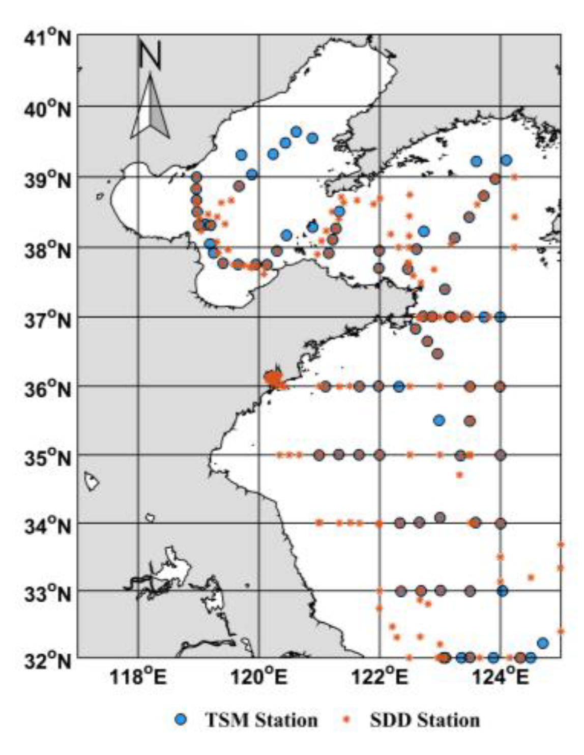
Figure 2.
Scatter plots of suspended matter concentration retrieved using three different atmospheric correction algorithms compared against in-situ measured data. (a) GDPS2.0 atmospheric correction algorithm; (b) NASA standard atmospheric correction algorithm; (c) MUMM atmospheric correction algorithm.
Figure 2.
Scatter plots of suspended matter concentration retrieved using three different atmospheric correction algorithms compared against in-situ measured data. (a) GDPS2.0 atmospheric correction algorithm; (b) NASA standard atmospheric correction algorithm; (c) MUMM atmospheric correction algorithm.
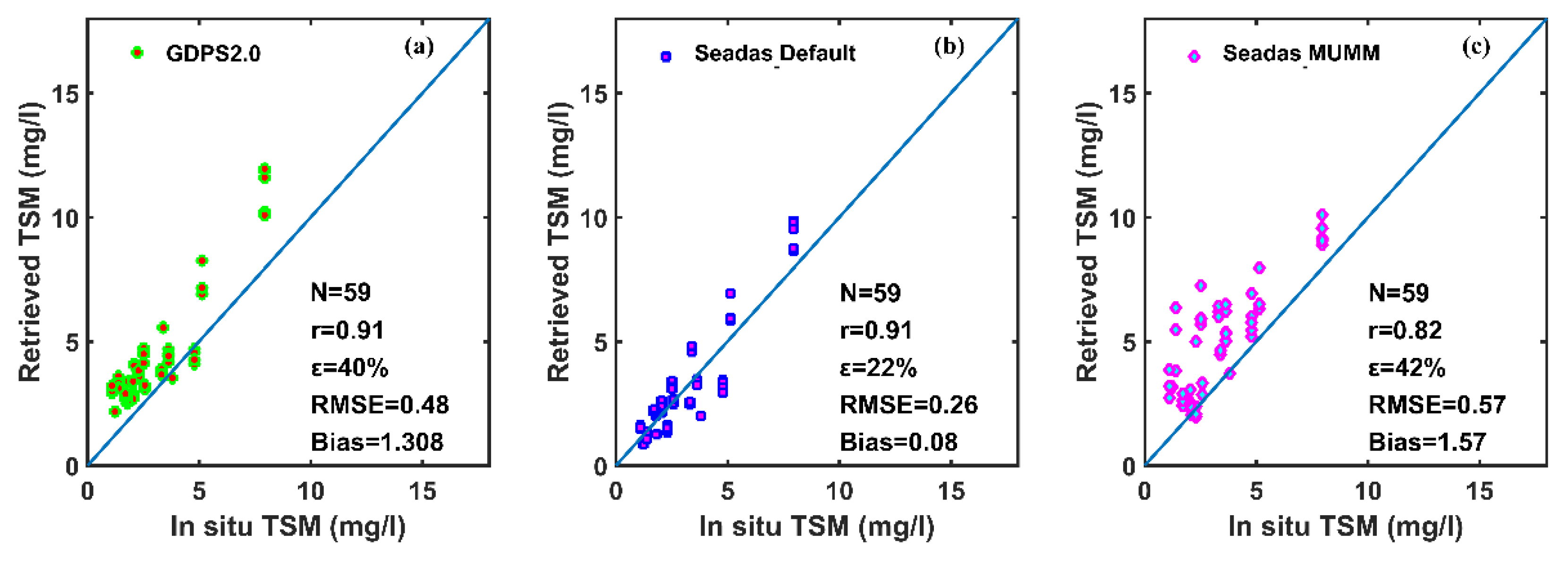
Figure 3.
Scatter plots of transparency data retrieved using three different atmospheric correction algorithms compared against in-situ measured data. (a) GDPS2.0 atmospheric correction algorithm; (b) NASA standard atmospheric correction algorithm; (c) MUMM atmospheric correction algorithm.
Figure 3.
Scatter plots of transparency data retrieved using three different atmospheric correction algorithms compared against in-situ measured data. (a) GDPS2.0 atmospheric correction algorithm; (b) NASA standard atmospheric correction algorithm; (c) MUMM atmospheric correction algorithm.
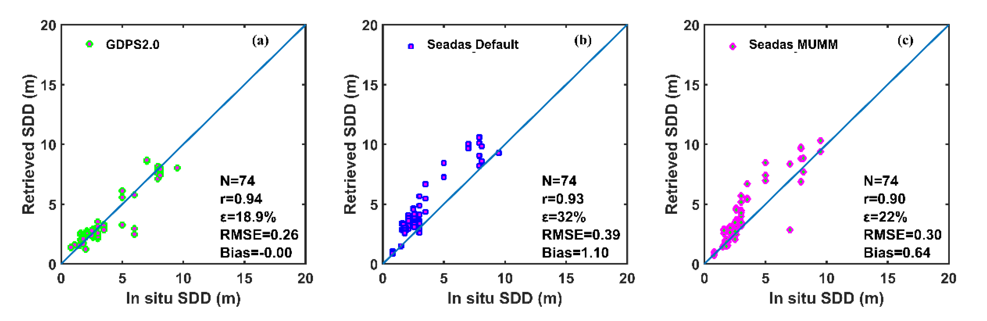
Figure 4.
Spatial distribution results suspended matter concentration retrieved from GOCI data at 05:16 UTC (13:16 local time) on March 9, 2018, using three different atmospheric correction algorithms. (a) GDPS2.0 atmospheric correction algorithm; (b) NASA standard atmospheric correction algorithm; (c) MUMM atmospheric correction algorithm.
Figure 4.
Spatial distribution results suspended matter concentration retrieved from GOCI data at 05:16 UTC (13:16 local time) on March 9, 2018, using three different atmospheric correction algorithms. (a) GDPS2.0 atmospheric correction algorithm; (b) NASA standard atmospheric correction algorithm; (c) MUMM atmospheric correction algorithm.
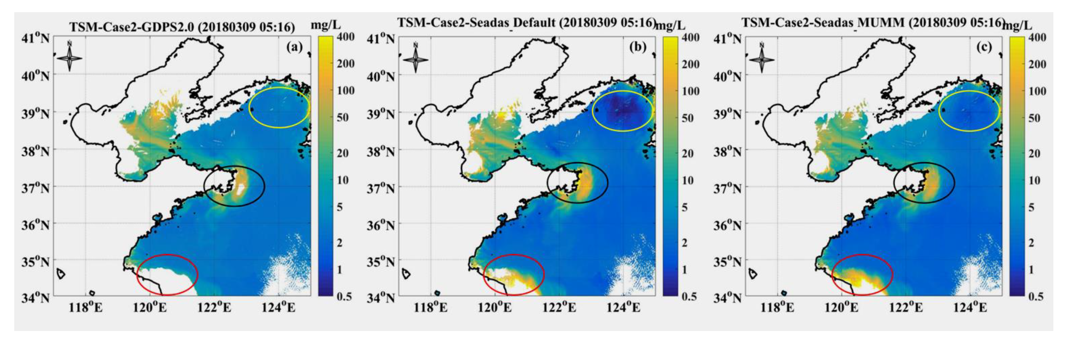
Figure 5.
Spatial distribution of transparency data retrieved from GOCI data at 05:16 UTC (13:16 local time) on March 9, 2018, using three different atmospheric correction algorithms. (a) GDPS2.0 atmospheric correction algorithm; (b) NASA standard atmospheric correction algorithm; (c) MUMM atmospheric correction algorithm.
Figure 5.
Spatial distribution of transparency data retrieved from GOCI data at 05:16 UTC (13:16 local time) on March 9, 2018, using three different atmospheric correction algorithms. (a) GDPS2.0 atmospheric correction algorithm; (b) NASA standard atmospheric correction algorithm; (c) MUMM atmospheric correction algorithm.
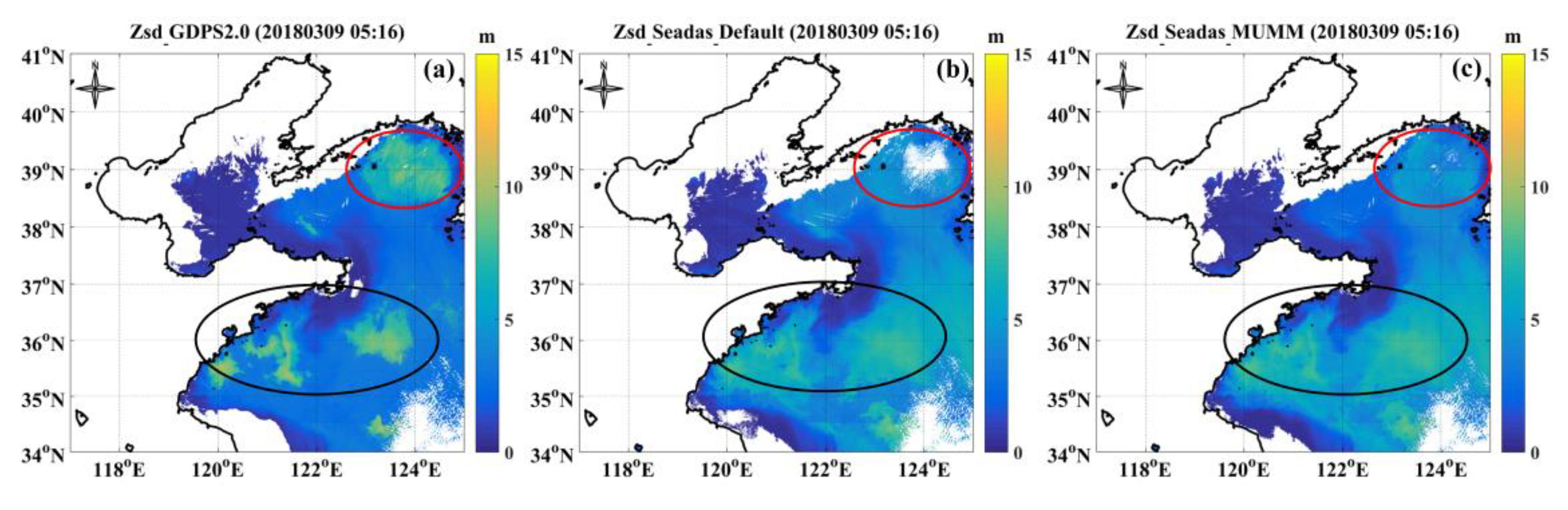
Figure 6.
Variation rates of suspended matter concentration data relative to TSM_GDPS2.0 obtained using the NASA standard atmospheric correction algorithm (a) and MUMM atmospheric correction algorithm (b) at 13:16 (local time) on March 9, 2018.
Figure 6.
Variation rates of suspended matter concentration data relative to TSM_GDPS2.0 obtained using the NASA standard atmospheric correction algorithm (a) and MUMM atmospheric correction algorithm (b) at 13:16 (local time) on March 9, 2018.
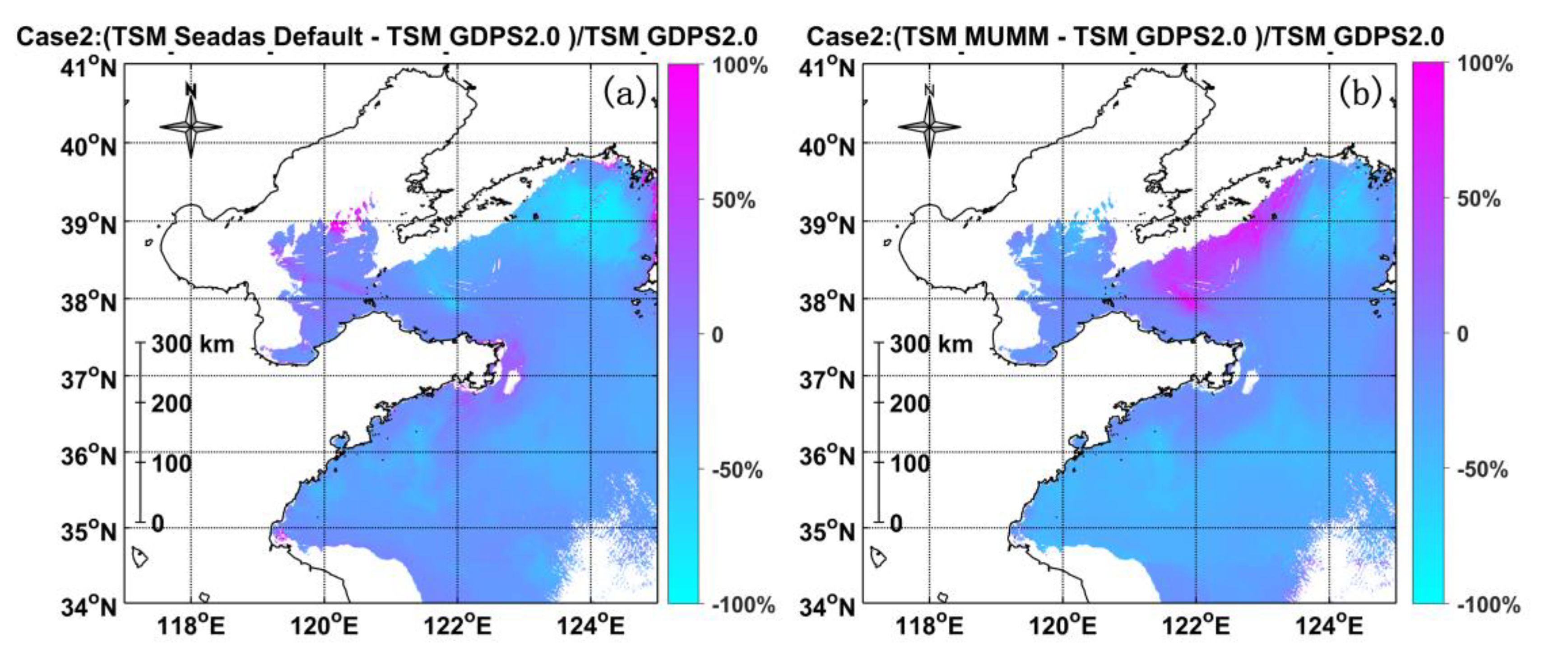
Figure 7.
Variation rates of transparency data relative to Zsd_GDPS2.0 obtained using the NASA standard atmospheric correction algorithm (a) and MUMM atmospheric correction algorithm (b) at 13:16 (local time) on March 9, 2018.
Figure 7.
Variation rates of transparency data relative to Zsd_GDPS2.0 obtained using the NASA standard atmospheric correction algorithm (a) and MUMM atmospheric correction algorithm (b) at 13:16 (local time) on March 9, 2018.
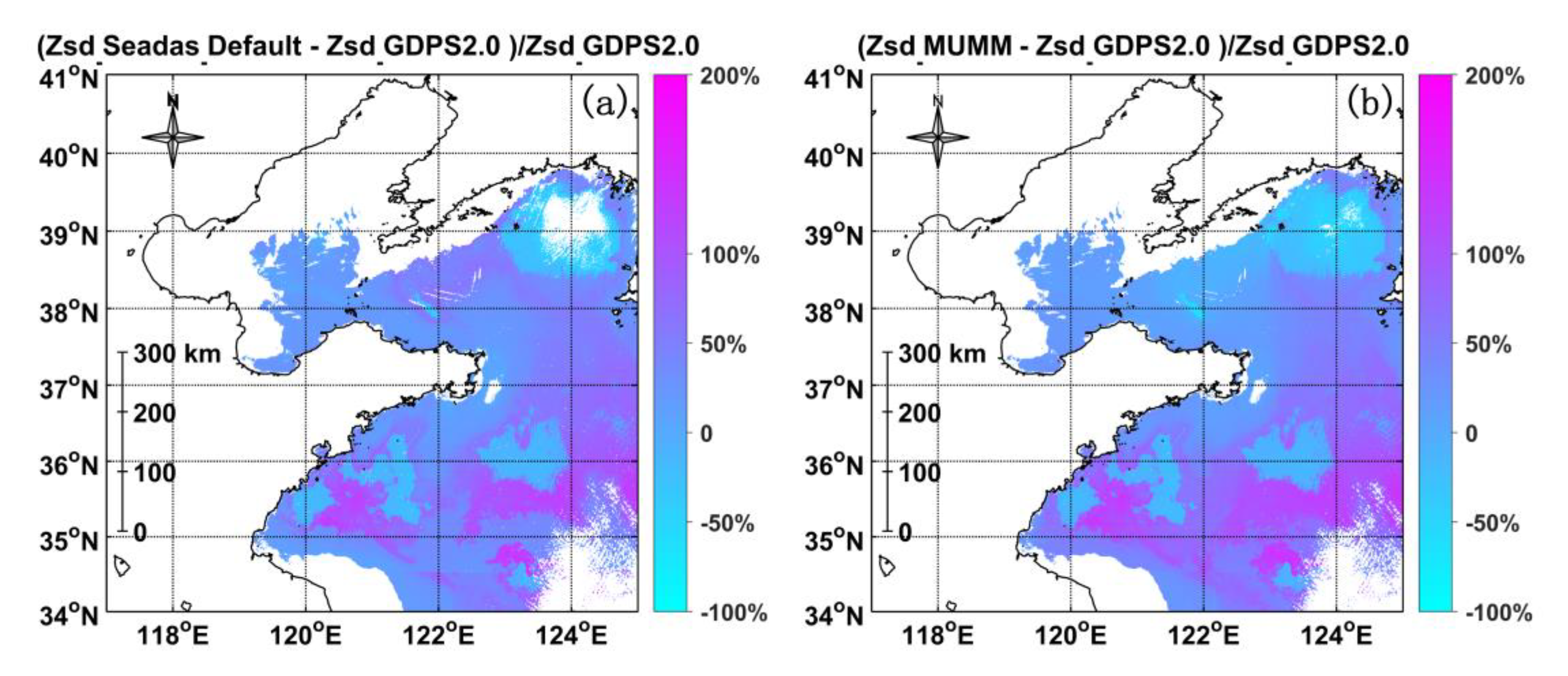
Figure 8.
Spatial distribution of the occurrence times of maximum and minimum suspended matter concentration on March 9, 2018, retrieved using different AC algorithms (local time).
Figure 8.
Spatial distribution of the occurrence times of maximum and minimum suspended matter concentration on March 9, 2018, retrieved using different AC algorithms (local time).
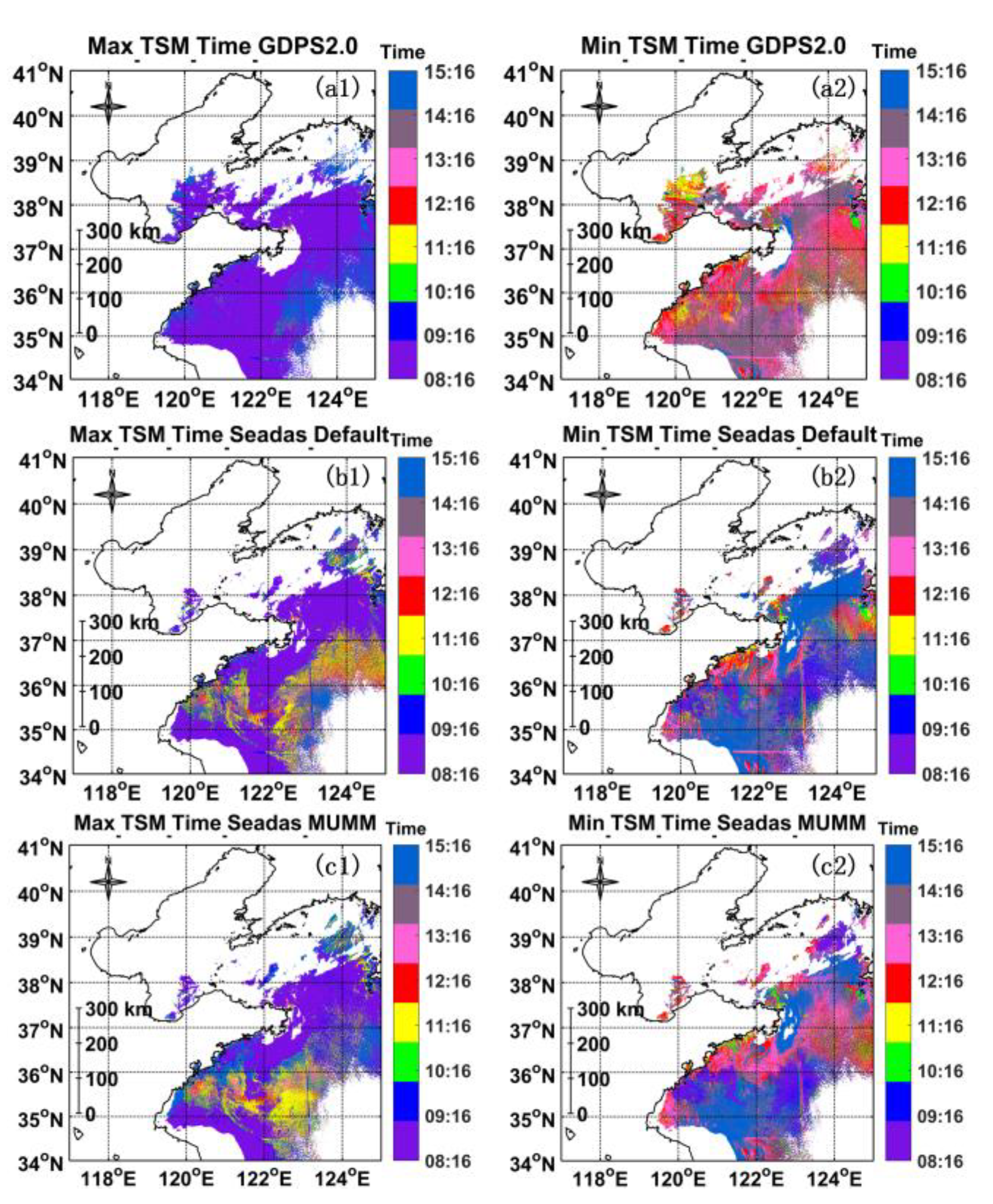
Figure 9.
Spatial distribution of the occurrence times of maximum and minimum transparency on March 9, 2018, retrieved using different AC algorithms (local time).
Figure 9.
Spatial distribution of the occurrence times of maximum and minimum transparency on March 9, 2018, retrieved using different AC algorithms (local time).
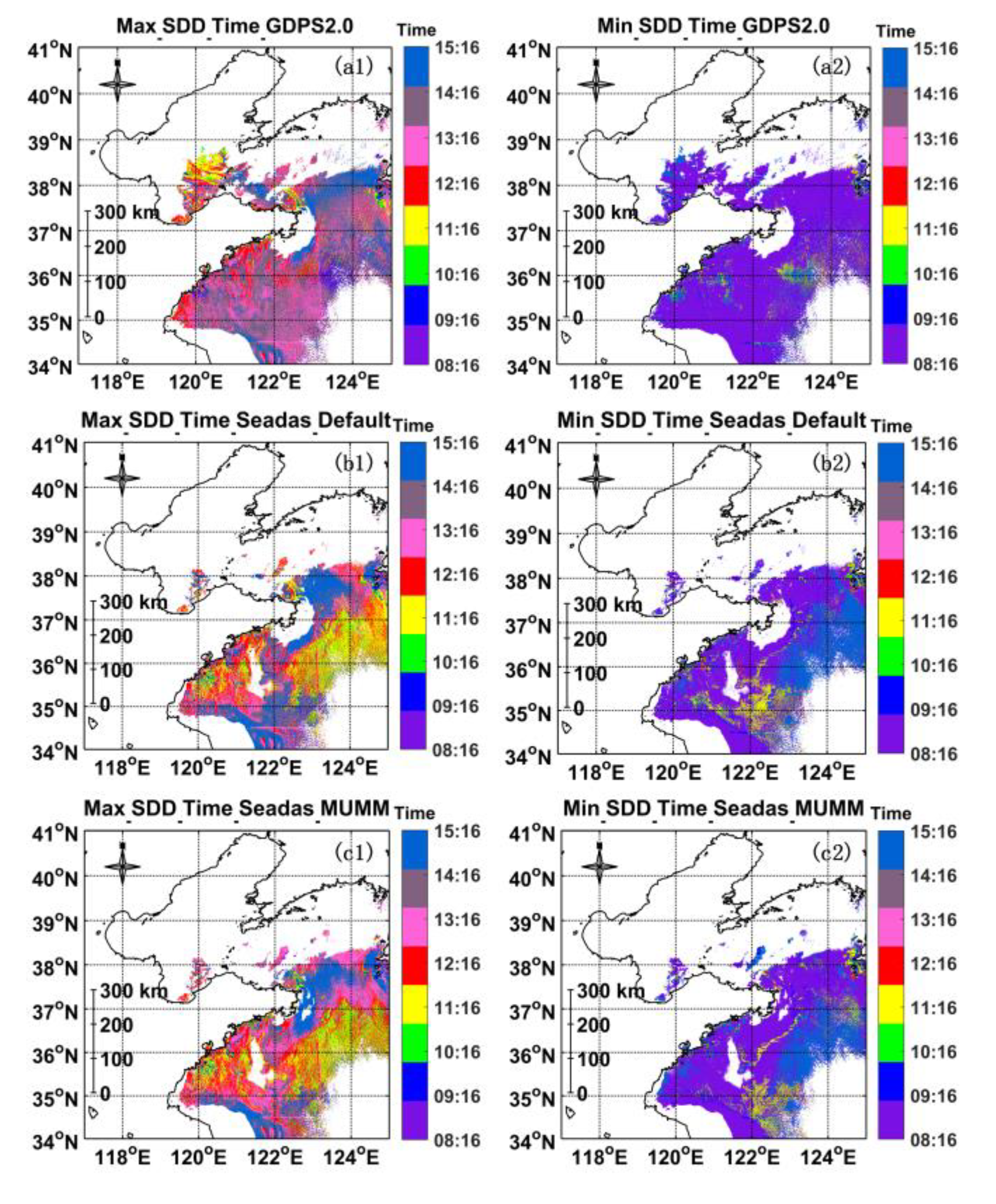
Figure 10.
Frequency statistics of the occurrence times of extreme values of suspended matter concentration and transparency retrieved using different atmospheric correction algorithms on March 9, 2018 (local time).
Figure 10.
Frequency statistics of the occurrence times of extreme values of suspended matter concentration and transparency retrieved using different atmospheric correction algorithms on March 9, 2018 (local time).
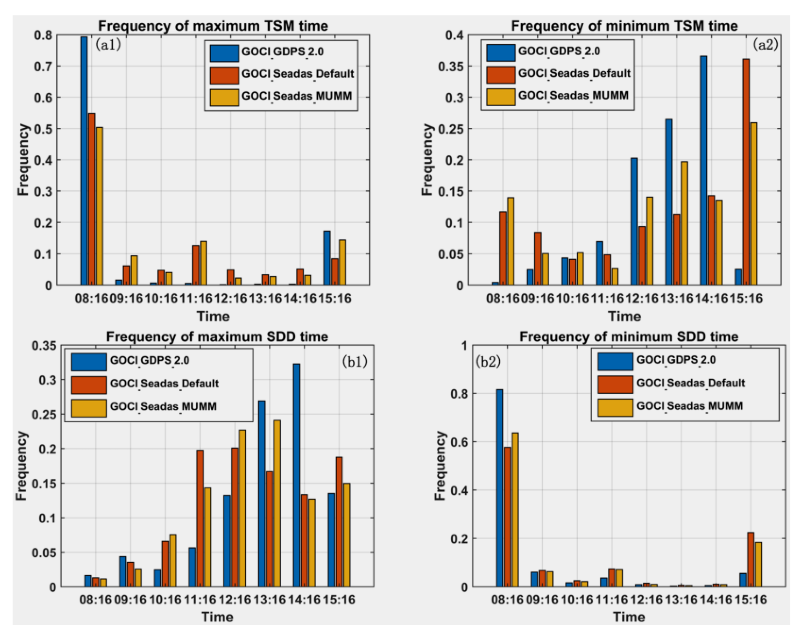
Figure 11.
Schematic diagram of region and transect selection.
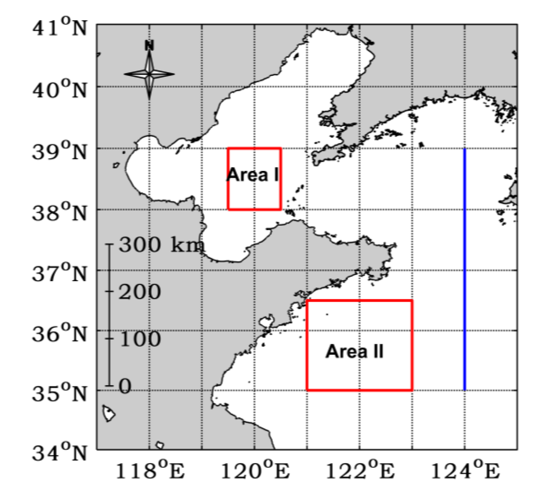
Figure 12.
Comparison of transparency (a) and suspended matter concentration (b) along the longitudinal transect retrieved from GOCI data at 13:16 (local time) on March 9, 2018, using three different atmospheric correction algorithms. Red curve: GDPS2.0 atmospheric correction algorithm; Blue curve: NASA standard atmospheric correction algorithm; Green curve: MUMM atmospheric correction algorithm.
Figure 12.
Comparison of transparency (a) and suspended matter concentration (b) along the longitudinal transect retrieved from GOCI data at 13:16 (local time) on March 9, 2018, using three different atmospheric correction algorithms. Red curve: GDPS2.0 atmospheric correction algorithm; Blue curve: NASA standard atmospheric correction algorithm; Green curve: MUMM atmospheric correction algorithm.
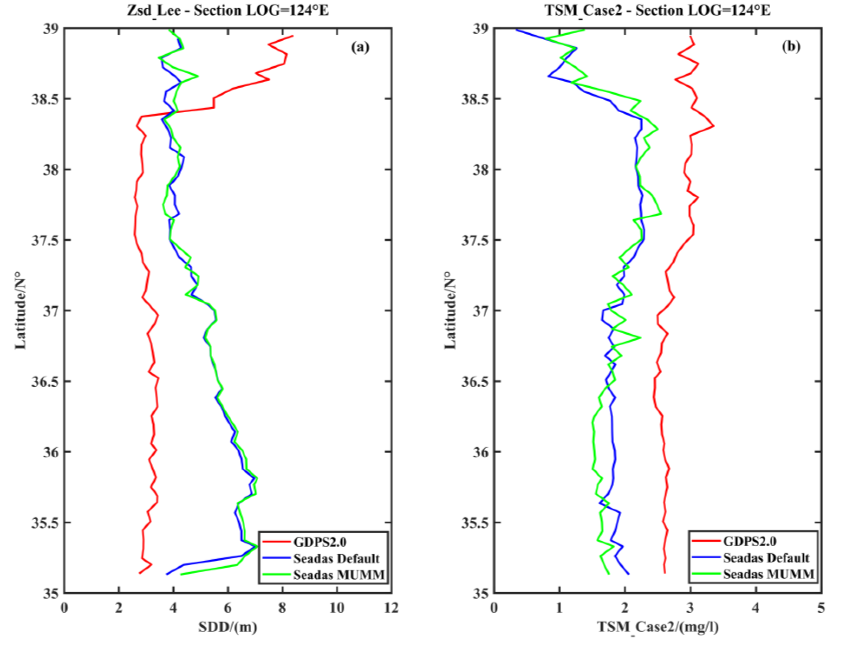
Figure 13.
Hourly variation of transparency (a) and suspended matter concentration (b) retrieved from GOCI data in Sea Area I at 08:16-15:16 (local time) on March 9, 2018, using three different atmospheric correction algorithms. Red curve: GDPS2.0 atmospheric correction algorithm; Blue curve: NASA standard atmospheric correction algorithm; Green curve: MUMM atmospheric correction algorithm.
Figure 13.
Hourly variation of transparency (a) and suspended matter concentration (b) retrieved from GOCI data in Sea Area I at 08:16-15:16 (local time) on March 9, 2018, using three different atmospheric correction algorithms. Red curve: GDPS2.0 atmospheric correction algorithm; Blue curve: NASA standard atmospheric correction algorithm; Green curve: MUMM atmospheric correction algorithm.
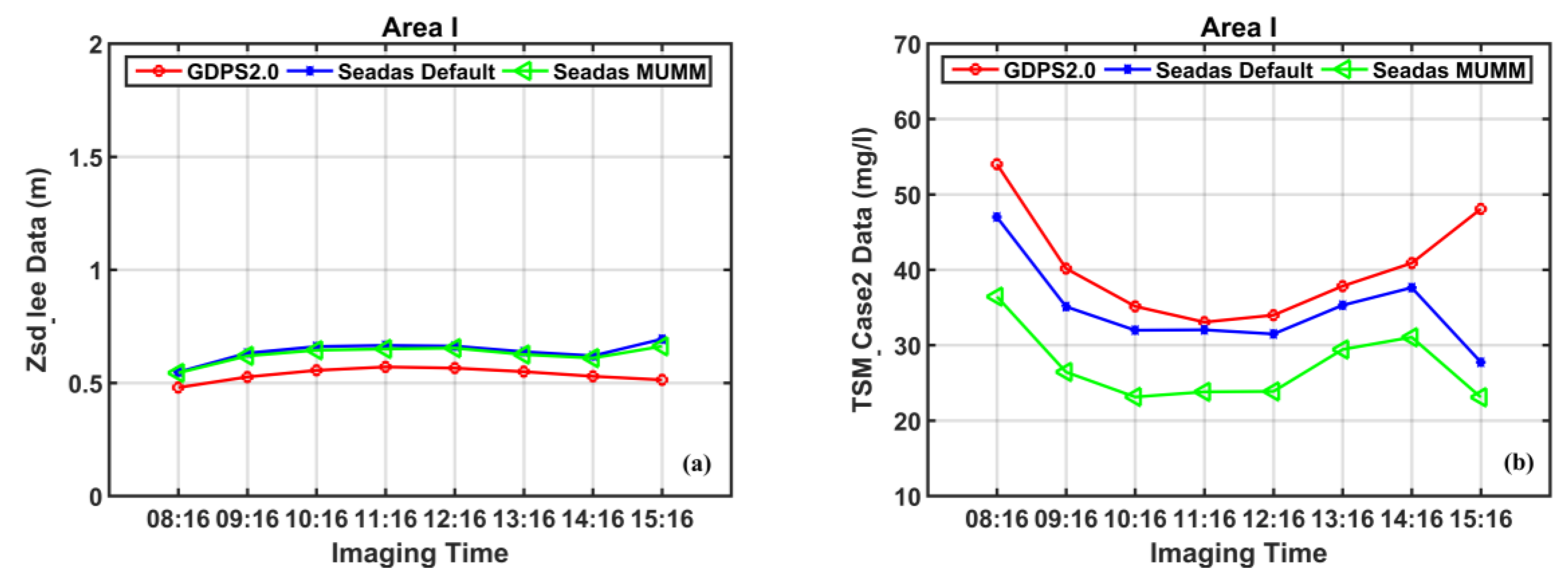
Figure 14.
Hourly variation of transparency (a) and suspended matter concentration (b) retrieved from GOCI data in Sea Area II at 08:16-15:16 (local time) on March 9, 2018, using three different atmospheric correction algorithms. Red curve: GDPS2.0 atmospheric correction algorithm; Blue curve: NASA standard atmospheric correction algorithm; Green curve: MUMM atmospheric correction algorithm.
Figure 14.
Hourly variation of transparency (a) and suspended matter concentration (b) retrieved from GOCI data in Sea Area II at 08:16-15:16 (local time) on March 9, 2018, using three different atmospheric correction algorithms. Red curve: GDPS2.0 atmospheric correction algorithm; Blue curve: NASA standard atmospheric correction algorithm; Green curve: MUMM atmospheric correction algorithm.
Disclaimer/Publisher’s Note: The statements, opinions and data contained in all publications are solely those of the individual author(s) and contributor(s) and not of MDPI and/or the editor(s). MDPI and/or the editor(s) disclaim responsibility for any injury to people or property resulting from any ideas, methods, instructions or products referred to in the content. |
© 2026 by the authors. Licensee MDPI, Basel, Switzerland. This article is an open access article distributed under the terms and conditions of the Creative Commons Attribution (CC BY) license (http://creativecommons.org/licenses/by/4.0/).
Copyright: This open access article is published under a Creative Commons CC BY 4.0 license, which permit the free download, distribution, and reuse, provided that the author and preprint are cited in any reuse.