

Submitted:
17 August 2026
Posted:
18 August 2026
You are already at the latest version
Abstract
The objective of this research is to estimate the impact of fiscal policy (approximated by the ratio of public investment to government consumption and the shares of direct and indirect tax revenues in GDP) on economic growth and income inequality in Por-tugal during 1995–2025. Annual data and autoregressions with distributed lag (ARDLs) accounting for trade openness, corruption control and tourism are employed in the study. The empirical results indicate that Portugal’s growth is affected by cor-ruption control and tourism in the long term and by the ratio of government invest-ment to government consumption in the short term. The results also show that income distribution in Portugal is influenced by corruption control, indirect tax revenues, tourism and trade openness in the long run and by direct tax revenues, tourism and trade openness in the short run. It is interesting that while Portugal’s economic growth is influenced by the structure of government expenditures in the short term, Portugal’s income inequality is impacted by direct taxes in the short run and by indirect taxes in the long run. It may be inferred that foreign trade, corruption control and tourism are essential determinants of economic growth and income distribution in Portugal, which emphasizes the importance of economic freedom and institutional quality for eco-nomic wellbeing and social resilience.
Keywords:
Portugal
; fiscal policy
; economic growth
; income distribution
1. Introduction
Whereas economic growth is the main source of a nation’s wealth, income distribution is a key determinant of social sustainability.
The impact of fiscal policy on economic growth is a central, albeit highly debated, topic in macroeconomics. While there is broad consensus that fiscal policy—comprising government spending, taxation, and debt management—influences economic performance, the nature, direction, and magnitude of these effects remain subjects of extensive empirical and theoretical investigation [1].
The relationship between fiscal policy and income distribution is a central pillar of modern macroeconomic policy. Governments employ fiscal instruments—primarily taxation and government spending—not only to stabilize the economy but also to correct market-driven income disparities.
The goal of this study is to explore the effects of fiscal policy on economic growth and income disparity in Portugal. Yearly data for the period 1995–2025 and autoregressions with distributed lag (ARDLs), which control for trade openness, corruption control and tourism, are utilized in the research. The empirical results imply that whereas Portuguese economic growth is affected by the ratio of government investment to government consumption in the short run, Portuguese income disparity is influenced by direct taxes in the short term and by indirect taxes in the long term.
The aim of the paper is achieved by the fulfillment of the following tasks:
- Systematization of theoretical and empirical studies about the impacts of fiscal policy on economic growth and income disparity (section two);
- Empirical estimation of the effects of fiscal policy on economic growth and income distribution in Portugal (section three);
- Results interpretation and policy recommendations (conclusion section).
2. Theoretical Background
2.1. Impact of Fiscal Policy on Economic Growth
The fiscal policy, together with the monetary policy, is the main instrument of government economic regulation. Traditionally, the government intervention is viewed as an instrument in a closed economy, i.e., economy that does not interact with its physical environment. If we drop this constraint and define the economic system as an open one, then the fiscal and monetary policies become the necessary feed back, guaranteeing the equilibrium convergence [2]. In empirical terms this means that economic growth should be involved in equilibrium interactions with fiscal variables in short and long run.
In the domain of the main stream economics, the impact of fiscal policy on economic growth remains one of the most debated subjects. While early neoclassical models viewed fiscal policy primarily as a tool for short-term stabilization, modern research emphasizes its potential for permanent effects on growth via human capital accumulation, infrastructure development, and institutional quality [3,4].
The literature is divided by the “Keynesian” and “Neoclassical” views. Keynesian theory posits that fiscal expansion, particularly through government spending, can stimulate aggregate demand and economic growth during downturns (Spilimbergo et al., 2009). Conversely, neoclassical theory suggests that excessive government spending and distortionary taxation can crowd out private investment, ultimately hindering long-term growth [3].
Endogenous growth models have further evolved this discussion by suggesting that the composition of fiscal policy—specifically the distinction between productive investment (e.g., infrastructure, R&D) and unproductive consumption—is a primary determinant of growth [5,6].
Early neoclassical growth models, such as those derived from the Solow [7] framework, primarily viewed fiscal policy as having temporary effects on growth by shifting the economy toward different steady-state levels of capital [3]. In contrast, endogenous growth theory suggests that fiscal policy can exert permanent effects on long-term growth rates by influencing the accumulation of human and physical capital, as well as research and development [8].
Empirical research generally suggests that the relationship between fiscal policy and growth is non-linear and context-dependent, relying on several critical factors:

- Institutional Quality: The effectiveness of fiscal policy is often mediated by institutional frameworks. Factors such as fiscal transparency, corruption levels, and regulatory quality determine whether fiscal interventions effectively stimulate growth or result in inefficiencies [4];
- Debt Sustainability: For countries with high levels of public debt, fiscal consolidation (reducing budget deficits) can sometimes be expansionary by improving market confidence and reducing interest rates, a phenomenon frequently discussed in literature regarding industrialized nations [8].
Fiscal multipliers represent the change in output resulting from a unit change in fiscal policy. Research indicates that these multipliers are not static but vary significantly based on:
- Economic Openness: Smaller, more open economies often exhibit smaller multipliers, as stimulus “leaks” out through imports [12];
- Monetary Policy Environment: The effectiveness of fiscal policy is often mediated by the central bank’s reaction function; if monetary policy is accommodative, fiscal multipliers are typically larger [13].
The “non-Keynesian” effects of fiscal consolidation have been a major focus in recent literature. While austerity is often contractionary in the short term, some studies suggest that credible, spending-based consolidation can foster growth by reducing risk premiums and boosting private sector confidence [14,15].
Furthermore, institutional quality acts as a significant moderator. In countries with high fiscal transparency and robust regulatory frameworks, fiscal policy tends to be more effective and predictable. Conversely, in environments of high corruption or fiscal opacity, the link between public spending and growth is often weak or even negative [4].
As of 2026, the global fiscal landscape is defined by high public debt and geopolitical fragmentation. Recent analysis from the International Monetary Fund (2026) highlights that fiscal rules are increasingly essential for maintaining stability in an era of heightened geopolitical risks. Protecting public investment during periods of consolidation is now considered vital for long-term growth, as cutting capital expenditure to meet debt targets often leads to deeper, more persistent output losses [6].
In summary, the literature underscores that there is no “one-size-fits-all” approach to fiscal policy. Its impact on growth is highly heterogeneous, shaped by the mix of fiscal instruments, the prevailing macroeconomic environment, and the institutional quality of the nation in question.
2.2. Impact of Fiscal Policy on Income Distribution
Fiscal policy is a primary mechanism through which governments influence income distribution, acting on household welfare through both direct and indirect channels [7]. The academic literature distinguishes between predistribution—policies that shape market incomes before taxes and transfers—and redistribution, which reallocates resources after market incomes are realized [16,17].
Public expenditure on health and education acts as a long-term investment in human capital. By enhancing the earning potential of low-income households, these policies address inequality at the “pre-production” stage [17,18].
Fiscal policy influences income distribution through two primary channels: direct redistribution and indirect structural effects.
Progressive tax systems and social transfer programs (cash transfers, unemployment benefits, and pensions) directly alter the Gini coefficient by narrowing the gap between market income and disposable income. Direct redistribution involves progressive taxation and cash transfers (e.g., unemployment benefits, social pensions). While effective in many advanced economies, the redistributive impact varies significantly based on administrative capacity and policy design [8,19]. The so-called flat tax systems are not appropriate for dveloped market economies as a result of the law of diminishing marginal utility of income [20].
Public investment in human capital—specifically education and healthcare—is widely recognized as a “pre-distributive” tool. By improving access to quality services, these expenditures enhance the earning potential of low-income households, thereby reducing inequality in market incomes over the long term [21,22].
Research indicates that the effectiveness of fiscal policy in reducing inequality is highly heterogeneous across countries:
- Development Status: In advanced economies, social benefits are often the primary driver of inequality reduction. Conversely, in many developing nations, the tax side (specifically progressive income taxation) often plays a more significant role due to more limited or inefficient social safety nets [19];
- The Role of Composition: Not all spending is equalizing. Research has shown that while basic education and health spending are generally pro-poor, tertiary education subsidies are frequently regressive, as they predominantly benefit households in the upper income quintiles [23];
- Institutional Quality: The relationship between fiscal policy and inequality is moderated by institutional quality. While fiscal intervention can reduce inequality, corruption or weak administrative capacity can undermine the redistributive impact, sometimes leading to outcomes where fiscal systems are net poverty-increasing rather than poverty-reducing [24];
- The Equity-Efficiency Trade-off: Contrary to older neoclassical arguments, contemporary literature suggests that the tension between equity and efficiency is not a zero-sum game. Well-designed fiscal systems can reduce inequality without necessarily hindering growth, particularly when revenue mobilization focuses on broadening the tax base and removing inefficient subsidies [23].
Classical models, such as the median voter theorem [25], suggest that higher pre-tax inequality should lead to greater redistribution. However, empirical evidence often shows the opposite: more egalitarian societies sometimes engage in more aggressive redistribution, while highly unequal societies may experience political capture that limits redistributive efforts [26].
The impact of fiscal policy is not uniform and is heavily mediated by institutional quality. In many developing nations, the lack of efficient tax administration and bureaucratic capacity limits the reach of redistributive policies [27].
Studies suggest that where governance is weak, fiscal policy may fail to achieve distributional goals; in extreme cases, spending might be captured by elites rather than reaching the intended beneficiaries [27].
Indirect taxes, such as VAT, are often regressive and can increase poverty if not offset by targeted direct transfers [28]. Conversely, prioritizing spending on basic education and healthcare is consistently linked to lower inequality [27].
Recent analysis emphasizes that the “predistribution vs. redistribution” debate is crucial for explaining the widening inequality gap, particularly in the United States compared to Europe [29]. As of 2026, governments face the dual pressure of high debt levels and the need for fiscal consolidation. Research warns that poorly designed austerity measures risk exacerbating income inequality, highlighting the importance of protecting social safety nets during fiscal adjustments [30,31].
3. Materials and Methods
3.1. Impact of Fiscal Policy on Economic Growth
3.1.1. Methodology
The influence of fiscal policy on the real economic growth of Portugal is estimated via an autoregressive distributed lag model (ARDL), which contains the following variables:
GDPGRi – percentage rate of change of the real GDP of Portugal in year i on previous year i-1;
GE_RATi – the ratio of government investments to government consumption in Portugal in year i;
TAX_RATIOi – ratio between direct tax revenue and indirect tax revenue of Portugal in year i;
CON_CORi – the score of the Control of Corruption index for Portugal in year i;
TRD_OPNi – trade openness of Portugal in year i. It is calculated as the percentage share of the sum of exports and imports in GDP;
TOURISMi – percentage rate of change of the number of tourist arrivals in Portugal in year i on previous year i-1.
The target (dependent variable) is GDPGR. The independent variables of interest to this study are GE_RAT and TAX_RATIO, which indicate the structure of government expenditure and tax revenue. The other regressors are control variables, which account for the influence of the external sector (TRD_OPN), the quality of governance (CON_COR) and the tourist industry (TOURISM).
3.1.2. Data
Yearly Eurostat and World Bank data for the period 1995-2025 are used in the empirical analysis. The data for CON_COR are obtained from the World Bank website, while the data for the other variables are taken from the Eurostat website.
3.1.3. Results
The unit root tests (see Table 1) show that GDPGR and TOURISM are stationary at level (integrated of order 0), whereas D(GE_RAT), TAX_RATIO, CON_COR and TRD_OPN are stationary at first difference (integrated of order 1). The different order of integration of the variables requires the application of an ARDL.
According to the Akaike information criterion (AIC), the optimum number of lags for each variable in the ARDL is as follows: GDPGR – 1; GE_RAT – 1; TAX_RATIO – 0; CON_COR – 0; TRD_OPN – 0; TOURISM – 0 (see Figure 1). The selected ARDL is expressed by the equation
(1) D(GDPGR) = C(1) + C(2)*GDPGR(-1) + C(3)*GE_RAT(-1) + C(4)*TAX_RATIO + C(5)*CON_COR + C(6)*TRD_OPN + C(7)*TOURISM + C(8)*D(GE_RAT).
The results from the estimation of the selected model - ARDL(1, 1, 0, 0, 0, 0), are shown in Table 2. They indicate that corruption control and tourism affect Portugal’s real economic growth in the long run.
The value of the coefficient of determination (R-squared = 0.86) implies that 86% of the variation of the real economic growth in Portugal can be explained by changes in the independent variables in the ARDL. The probability of the F-statistic (0.00) indicates that the alternative hypothesis of adequacy of the model used is confirmed. It should be made clear that this does not mean that the model is the best possible, but simply that it adequately reflects the relationship between the dependent and the independent variables.
The residuals in the ARDL are normally distributed (see Figure 2), homoscedastic (see Table 3) and serially uncorrelated (see Table 4).
The ARDL is dynamically stable (see Figure 3).
The CUSUM graph illustrates that the cumulative sum of recursive residuals fluctuates within the 5% confidence bands across the entire period under review. This outcome suggests that the estimated ARDL model does not exhibit structural instability or significant parameter shifts.
The results from the F-Bounds Test (see Table 5) suggest that a long-run relationship exists between the variables in the ARDL, which requires the estimation of an error correction model (ECM). The ECM has the form
(2) D(GDPGR) = C(1) + C(2)*D(GE_RAT) + C(3)*ECT(-1).
The results from the estimation of the ECM are shown in Table 6. The regression coefficient before the error correction term (ECT) is statistically significant and negative, which implies the existence of a long-run equilibrium relationship between the dependent variable and the independent variables in the ECM. The value of this coefficient of –0.98 means that each deviation from the long-term equilibrium is eliminated at a rate of 98 percent per annum.
The short-run regression coefficient before D(GE_RAT) is significant (at the 10 percent level) and positive, which suggests that in the short run, the real economic growth in Portugal depends on the ratio between government investment and government consumption. A rise in this ratio will result in an accelerated real output growth rate.
The value of the coefficient of determination (R-sq. = 0.86) implies that 86% of the variation of real economic growth in Portugal can be explained by changes in the independent variables in the ECM. The probability of the F-statistic (0.00) indicates that the alternative hypothesis of adequacy of the model used is confirmed. It should be made clear that this does not mean that the model is the best possible, but simply that it adequately reflects the relationship between the dependent and the independent variables.
3.2. Impact of Fiscal Policy on Income Distribution
3.2.1. Methodology
The influence of tourism on income disparity in Portugal is estimated via an autoregressive distributed lag model (ARDL), which contains the following variables:
INC_RATi – top 10 percent to bottom 50 percent income ratio of Portugal in year i;
DIR_TAXi – direct tax revenue (percentage of GDP) in Portugal in year i;
IND_TAXi – indirect tax revenue (percentage of GDP) in Portugal in year i;
CON_CORi – the score of the Control of Corruption index for Portugal in year i;
TRD_OPNi – trade openness of Portugal in year i. It is calculated as the percentage share of the sum of exports and imports in GDP;
TOURISMi – percentage rate of change of the number of tourist arrivals in Portugal in year i on previous year i-1.
The target (dependent variable) is INC_RAT. The independent variables of interest to this study are DIR_TAX and IND_TAX, which indicate the shares of direct tax and indirect tax revenues in GDP. The other regressors are control variables, which account for the influence of the external sector (TRD_OPN), the quality of governance (CON_COR) and the number of tourists (TOURISM).
3.2.2. Data
Yearly data from the World Inequality Database, the Eurostat and the World Bank for the period 1995-2025 are used in the empirical analysis. The data for INC_RAT and CON_COR are obtained from World Inequality Database and the World Bank website respectively, while the data for the other variables are taken from the Eurostat website.
3.2.3. Results
The unit root tests (see Table 7) show that TOURISM is stationary at level (integrated of order 0), while the other variables are stationary at first difference (integrated of order 1). The different order of integration of the variables requires the application of an ARDL.
According to the Akaike information criterion (AIC), the optimum number of lags for each variable in the ARDL is as follows: INC_RAT – 1; DIR_TAX – 1; IND_TAX – 0; CON_COR – 0; TRD_OPN – 1; TOURISM – 1 (see Figure 4). The selected ARDL is expressed by the equation
(3) D(INC_RAT) = C(1) + C(2)*INC_RAT(-1) + C(3)*DIR_TAX(-1) + C(4)*IND_TAX + C(5)*CON_COR + C(6)*TRD_OPN(-1) + C(7)*TOURISM(-1) + C(8)*D(DIR_TAX) + C(9)*D(TRD_OPN) + C(10)*D(TOURISM).
The results from the estimation of the selected model - ARDL(1, 1, 0, 0, 1, 1), are shown in Table 8. They indicate that income distribution in Portugal is affected by tourism, indirect tax revenue, corruption control and trade openness in the long run and by direct tax revenue and trade openness in the short run.
The value of the coefficient of determination (R-squared = 0.65) implies that 65% of the variation of income distribution in Portugal can be explained by changes in the independent variables in the ARDL. The probability of the F-statistic (0.02) indicates that the alternative hypothesis of adequacy of the model used is confirmed. It should be made clear that this does not mean that the model is the best possible, but simply that it adequately reflects the relationship between the dependent and the independent variables.
The ARDL is dynamically stable (see Figure 5).
The results from the F-Bounds Test (see Table 11) suggest that a long-run relationship exists between the variables in the ARDL, which requires the estimation of an error correction model (ECM). The ECM has the form
(4) D(INC_RAT) = C(1) + C(2)*D(DIR_TAX) + C(3)*D(TRD_OPN) + C(4)*D(TOURISM) + C(5)*ECT(-1).
The results from the estimation of the ECM are shown in Table 12. The regression coefficient before the error correction term (ECT) is statistically significant and negative, which implies the existence of a long-run equilibrium relationship between the dependent variable and the independent variables in the ECM. The value of this coefficient of –0.72 means that each deviation from the long-term equilibrium is eliminated at a rate of 72 percent per annum.
The short-run regression coefficient before D(TOURISM), D(DIR_TAX) and D(TRD_OPN) are also significant, which suggests that in the short run income distribution in Portugal depends on the number of tourist arrivals, direct tax revenues and trade openness. The signs of these coefficients - positive before D(TOURISM) and negative before D(TRD_OPN) and D(DIR_TAX) – suggest that a decrease in the number of tourists as well as a rise in trade openness and direct tax revenue will result in lower income inequality.
The value of the coefficient of determination (R-sq. = 0.65) implies that 65% of the variation of real economic growth in Portugal can be explained by changes in the independent variables in the ECM. The probability of the F-statistic (0.00) indicates that the alternative hypothesis of adequacy of the model used is confirmed. It should be made clear that this does not mean that the model is the best possible, but simply that it adequately reflects the relationship between the dependent and the independent variables.
4. Discussion
The empirical results from this investigation confirm the significance of fiscal policy for encouraging economic growth and mitigating income inequality. While the structure of government expenses affects Portuguese economic growth in the short run, direct taxes influence income distribution in the short term and indirect taxes impact on it in the long term. The results also indicate that foreign trade, tourism and corruption control impact on economic growth and income distribution in Portugal, which emphasizes the importance of economic freedom and institutional quality for the wealth and sustainability of the Portuguese society. There is another interesting point. Fiscal variables not only affect growth, but are involved in equilibrium convergence, error correction interdependencies. This seems to confirm the open system hypothesis.
5. Conclusions
This research has important implications for Portuguese policymakers since it estimates the effects of fiscal policy, trade openness, corruption control and tourism on economic growth and income distribution in Portugal. The empirical results indicate that Portugal’s economic growth can be encouraged by increasing the ratio of government investment to government consumption in the short run and by raising the number of tourist arrivals and corruption control in the long run. In the same time, income inequality can be alleviated by improved corruption control, lower indirect tax revenues, fewer tourist arrivals, and higher trade openness in the long term and by more direct tax revenues, fewer tourists and increased trade openness in the short term.
Funding
This research received no external funding.
Data Availability Statement
No new data is generated. Public Eurostat, WID and ECB macroeconomic data is used in the study.
Conflicts of Interest
The author declares no conflicts of interest.
Abbreviations
The following abbreviations are used in this manuscript:
| ARDL | Autoregression with distributed lag |
| IFS | Institute for Fiscal Studies |
| IMF | International Monetary Fund |
| R&D | Research and development |
References
- Andini, M. (2024). The Influence of Fiscal Policy on Economic Growth. ORGANIZE: Journal of Economics, Management and Finance, 3(1), 1–9. [CrossRef]
- Ganchev, G. (2026). Economics as an Open Physical System. Systems Research and Behavioral Science, 2026; 0:1–12 . [CrossRef]
- Easterly, W., & Rebelo, S. (1993). Fiscal policy and economic growth: An empirical investigation. Journal of Monetary Economics, 32(3), 417–458. [CrossRef]
- Macek, R., & Janků, J. (2015). The impact of fiscal policy on economic growth depending on institutional conditions. Acta Academica Karviniensia, 15(2), 95–107. https://aak.actavia.cz/pdfs/aak/2015/02/08.pdf.
- Kneller, R., Bleaney, M. F., & Gemmell, N. (1999). Fiscal policy and growth: Evidence from OECD countries. Journal of Public Economics, 74(2), 171–190. [CrossRef]
- Ardanaz, M., Cavallo, E. A., Izquierdo, A., & Puig, J. (2021). Output effects of fiscal consolidations: Does spending composition matter? Inter-American Development Bank. https://dx.doi.org/10.18235/0003881.
- Solow, R. M. (1956). A contribution to the theory of economic growth. The Quarterly Journal of Economics, 70(1), 65–94. [CrossRef]
- Clements, B. J., Gupta, S., & Inchauste, G. (Eds.). (2004). Helping countries develop: The role of fiscal policy. International Monetary Fund. https://www.imf.org/external/pubs/nft/2004/hcd/index.htm.
- Kim, J., Wang, M., Park, D., & Petalcorin, C. C. (2021). Fiscal policy and economic growth: Some evidence from China. Review of World Economics, 157(3), 555–582. [CrossRef]
- Baum, A., Poplawski-Ribeiro, M., & Weber, A. (2012). Fiscal multipliers and the state of the economy. IMF Working Papers WP/12/286. https://www.imf.org/external/pubs/ft/wp/2012/wp12286.pdf.
- Abiad, A., Furceri, D., & Topalova, P. (2016). The macroeconomic effects of public investment: Evidence from advanced economies. Journal of Macroeconomics, 50, 224–240. [CrossRef]
- Spilimbergo, A., Symansky, S., & Schindler, M. (2009). Fiscal multipliers. IMF Staff Position Note. https://www.imf.org/external/pubs/ft/spn/2009/spn0911.pdf.
- Uddin, G. S., Le, A. H., Yago, N., Beirne, J., & Park, D. (2026). Global fragmentation, fiscal policy, and economic growth: A cross-country analysis (Working Paper No. 62). The South East Asian Central Banks (SEACEN) Research and Training Centre. https://www.seacen.org/publication-doc/WP03_2026_Final.pdf.
- Alesina, A., & Ardagna, S. (2010). Large changes in fiscal policy: Taxes versus spending. Tax Policy and the Economy, 24(1), 35–68. [CrossRef]
- Kleis, M., & Moessinger, M.-D. (2016). The long-run effect of fiscal consolidation on economic growth: Evidence from quantitative case studies (Discussion Paper No. 16-047). ZEW - Leibniz Centre for European Economic Research. https://www.zew.de/publikationen/the-long-run-effect-of-fiscal-consolidation-on-economic-growth-evidence-from-quantitative-case-studies.
- Hacker, J. S. (2011). The institutional foundations of middle-class democracy. Policy Network 6(5): 33-37. https://assets.website-files.com/64a8727f61fabfaa63b7b770/64aab85cf813ccbee57ce07f_hacker_pn.pdf.
- Blanchard, O., & Rodrik, D. (Eds.). (2021). Combating inequality: Rethinking government’s role. MIT Press. [CrossRef]
- Malhotra, S. and Voegel, S. (2025, December 17). The predistribution solution. Roosevelt Institute. https://rooseveltinstitute.org/publications/the-predistribution-solution/.
- Carranza, R., & Nolan, B. (2024). Assessing income redistribution: What are the key analytic choices? Fiscal Studies, 45(4), 501–519. [CrossRef]
- Ganchev, G. & Tanchev, S. (2019). Why Post-Communist Countries Choose the Flat Tax: A Comparative Welfare Approach, Acta Oeconomica, Vol. 69 (1) pp. 41–62 (2019) https://ideas.repec.org/a/aka/aoecon/v69y2019i1p41-62.html.
- Balseven, H., & Tugcu, C. T. (2017). Analyzing the effects of fiscal policy on income distribution: A comparison between developed and developing countries. International Journal of Economics and Financial Issues, 7(2), 377–383. https://www.econjournals.com/index.php/ijefi/article/view/4235.
- International Monetary Fund. (2014). Fiscal policy and income inequality (IMF Policy Paper). https://www.imf.org/external/np/pp/eng/2014/012314.pdf.
- Institute for Fiscal Studies. (2022). Fiscal policy and income inequality: The role of taxes and social spending. https://ifs.org.uk/publications/fiscal-policy-and-income-inequality-role-taxes-and-social-spending.
- Nguyen, V. B. (2023). From fiscal policy to income inequality in advanced economies: Does institutional quality hinder? Romanian Journal of Economic Forecasting, 26(1), 165–184. https://ipe.ro/new/rjef/rjef1_2023/rjef1_2023p165-184.pdf.
- Meltzer, A. H., & Richard, S. F. (1981). A rational theory of the size of government. Journal of Political Economy, 89(5), 914–927. https://www.jstor.org/stable/1830813.
- Bjorvatn, K., & Cappelen, A. (2003). Redistributive tax policies and inequality: An assessment of recent country comparative studies. CESifo DICE Report, 1(2), 26–31. https://www.ifo.de/DocDL/dicereport1-03-research-reports-3.pdf.
- Malla, M. H., & Pathranarakul, P. (2022). Fiscal Policy and Income Inequality: The Critical Role of Institutional Capacity. Economies, 10(5), 115. [CrossRef]
- Amjad, B., Carrasco Nunez, H., Finn, A. J., & Goldman, M. S. (2024). Fiscal policy, poverty, and inequality in a constrained environment: The case of the West Bank and Gaza (World Bank Policy Research Working Paper No. 10687). World Bank. [CrossRef]
- Blanchet, T., Chancel, L., & Gethin, A. (2022). Why is Europe more equal than the United States? American Economic Journal: Applied Economics, 14(4), 1–43. https://www.aeaweb.org/articles?id=10.1257/app.20200703.
- International Monetary Fund. (2026). Fiscal monitor: Fiscal policy under pressure: High debt, rising risks. https://www.imf.org/-/media/files/publications/fiscal-monitor/2026/april/english/text.pdf.
- Woo, J., Bova, E., Kinda, T., & Zhang, Y. S. (2013). Distributional consequences of fiscal consolidation and the role of fiscal policy: What do the data say? (IMF Working Paper No. 13/195). International Monetary Fund. https://www.imf.org/external/pubs/ft/wp/2013/wp13195.pdf.
Figure 1.
Model selection graph. Source: Own processing.
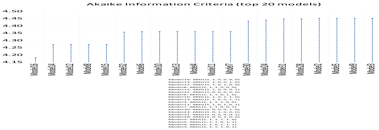
Figure 2.
Normal distribution test on the ARDL residuals. Source: Own processing.
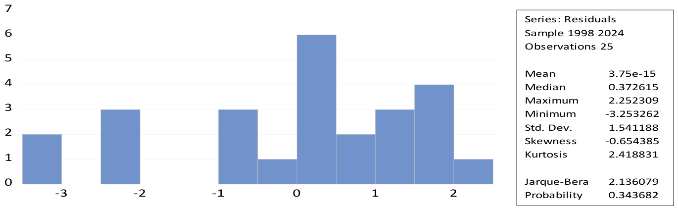
Figure 3.
CUSUM test for dynamic stability of the ARDL. Source: Own processing.
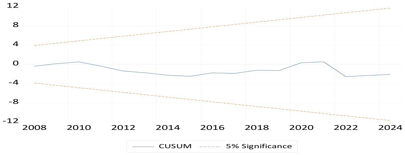
Figure 4.
Model selection graph. Source: Own processing.
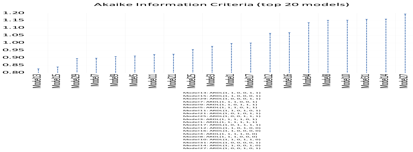
Figure 5.
CUSUM test for dynamic stability of the ARDL. Source: Own processing.
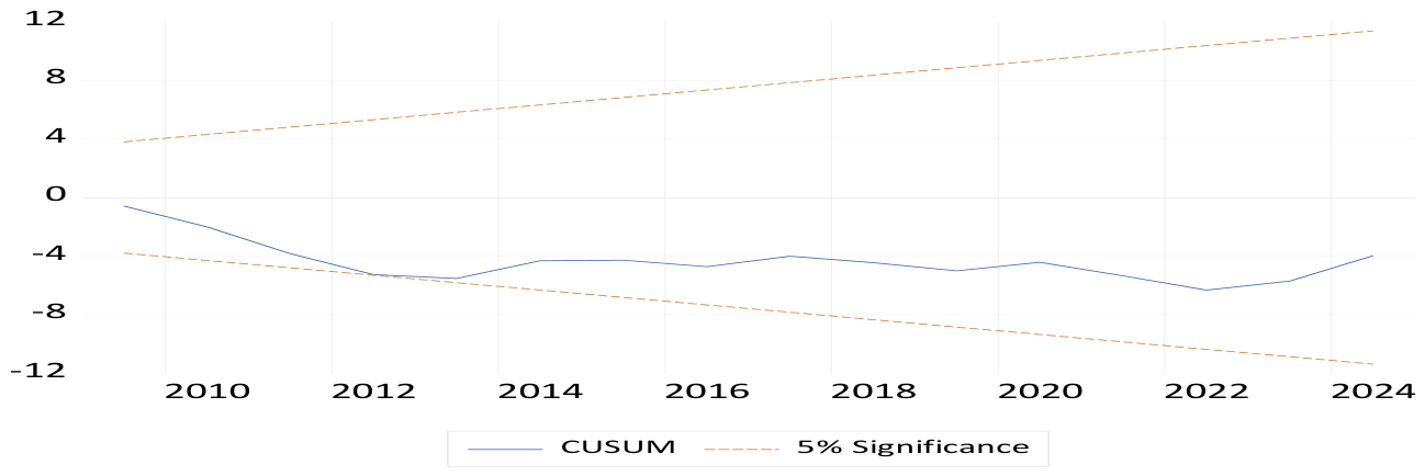

Table 1.
Augmented Dickey-Fuller unit root test on the level values and the first differences of variables in the ARDL.
Table 1.
Augmented Dickey-Fuller unit root test on the level values and the first differences of variables in the ARDL.
| Variable | Probability |
|---|---|
| GDPGR | 0.0023 |
| GE_RAT | 0.5509 |
| D(GE_RAT) | 0.0001 |
| TAX_RATIO | 0.0896 |
| D(TAX_RATIO) | 0.0000 |
| CON_COR | 0.0832 |
| D(CON_COR) | 0.0182 |
| TRD_OPN | 0.6352 |
| D(TRD_OPN) | 0.0001 |
| TOURISM | 0.0002 |
Source: Own processing.
Table 2.
Results from the econometric estimation of the selected ARDL.
| Variable | Coefficient | Standard Error | t-Statistic | Probability |
|---|---|---|---|---|
| C | -24.72446 | 15.09635 | -1.637777 | 0.1198 |
| GDPGR(-1)* | -0.978613 | 0.149404 | -6.550130 | 0.0000 |
| GE_RAT(-1) | 0.228587 | 14.15295 | 0.016151 | 0.9873 |
| TAX_RATIO** | -2.407823 | 7.445106 | -0.323410 | 0.7503 |
| CON_COR** | 0.310451 | 0.175271 | 1.771269 | 0.0944 |
| TRD_OPN** | 0.082259 | 0.080207 | 1.025583 | 0.3195 |
| TOURISM** | 0.104553 | 0.023619 | 4.426655 | 0.0004 |
| D(GE_RAT) | 22.30256 | 15.62250 | 1.427592 | 0.1715 |
Source: Own processing.
Table 3.
Heteroscedasticity test on the ARDL residuals.
| F-statistic | 0.490800 | Probability F (7,17) | 0.8284 |
| Observations R-squared | 4.202959 | Probability Chi-Square (7) | 0.7561 |
Source: Own processing.
Table 4.
Serial correlation test on the ARDL residuals.
| F-statistic | 0.008904 | Probability F (1,16) | 0.9260 |
| Observations R-squared | 0.013905 | Probability Chi-Square (1) | 0.9061 |
Source: Own processing.
Table 5.
F-Bounds Test.
| Test Statistic | Value | Significance | I(0) | I(1) |
|---|---|---|---|---|
| Asymptotic: n=1000 | ||||
| F-statistic | 17.06110 | 10% | 2.26 | 3.35 |
| k | 5 | 5% | 2.62 | 3.79 |
| 2.5% | 2.96 | 4.18 | ||
| 1% | 3.41 | 4.68 |
Source: Own processing.
Table 6.
Results from the econometric estimation of the ECM.
| Variable | Coefficient | Standard Error | t-Statistic | Probability |
|---|---|---|---|---|
| C | -24.72446 | 2.188922 | -11.29527 | 0.0000 |
| D(GE_RAT) | 22.30256 | 11.52330 | 1.935432 | 0.0698 |
| ECT(-1)* | -0.978613 | 0.085025 | -11.50975 | 0.0000 |
Source: Own processing.
Table 7.
Augmented Dickey-Fuller unit root test on the level values and the first differences of variables in the ARDL.
Table 7.
Augmented Dickey-Fuller unit root test on the level values and the first differences of variables in the ARDL.
| Variable | Probability |
|---|---|
| INC_RAT | 0.6506 |
| D(INC_RAT) | 0.0008 |
| DIR_TAX | 0.2281 |
| D(DIR_TAX) | 0.0000 |
| IND_TAX | 0.2121 |
| D(IND_TAX) | 0.0002 |
| CON_COR | 0.0832 |
| D(CON_COR) | 0.0182 |
| TRD_OPN | 0.6352 |
| D(TRD_OPN) | 0.0001 |
Source: Own processing.
Table 8.
Results from the econometric estimation of the selected ARDL.
| Variable | Coefficient | Standard Error | t-Statistic | Probability |
|---|---|---|---|---|
| C | 11.15600 | 3.185058 | 3.502604 | 0.0029 |
| INC_RAT(-1)* | -0.722721 | 0.167798 | -4.307097 | 0.0005 |
| DIR_TAX(-1) | 0.053420 | 0.142961 | 0.373670 | 0.7136 |
| IND_TAX** | 0.531550 | 0.187478 | 2.835262 | 0.0119 |
| CON_COR** | -0.071696 | 0.021514 | -3.332478 | 0.0042 |
| TRD_OPN(-1) | -0.098690 | 0.026633 | -3.705624 | 0.0019 |
| TOURISM(-1) | 0.016264 | 0.006687 | 2.432091 | 0.0271 |
| D(DIR_TAX) | -0.281163 | 0.125699 | 2.236802 | 0.0399 |
| D(TRD_OPN) | -0.078469 | 0.031926 | -2.457850 | 0.0258 |
| D(TOURISM) | 0.006331 | 0.005571 | 1.136532 | 0.2725 |
Source: Own processing.
Table 9.
Heteroscedasticity test on the ARDL residuals.
| F-statistic | 0.355117 | Probability F (7,17) | 0.9405 |
| Observations R-squared | 4.328877 | Probability Chi-Square (7) | 0.8885 |
Source: Own processing.
Table 10.
Serial correlation test on the ARDL residuals.
| F-statistic | 0.870508 | Probability F (1,15) | 0.3656 |
| Observations R-squared | 1.426117 | Probability Chi-Square (1) | 0.2324 |
Source: Own processing.
Table 11.
F-Bounds Test.
| Test Statistic | Value | Significance | I(0) | I(1) |
|---|---|---|---|---|
| Asymptotic: n=1000 | ||||
| F-statistic | 3.532668 | 10% | 2.26 | 3.35 |
| k | 5 | 5% | 2.62 | 3.79 |
| 2.5% | 2.96 | 4.18 | ||
| 1% | 3.41 | 4.68 |
Source: Own processing.
Table 12.
Results from the econometric estimation of the ECM.
| Variable | Coefficient | Standard Error | t-Statistic | Probability |
|---|---|---|---|---|
| C | 11.15600 | 2.146622 | 5.197000 | 0.0001 |
| D(DIR_TAX) | -0.281163 | 0.086398 | 3.254292 | 0.0050 |
| D(TRD_OPN) | -0.078469 | 0.023569 | -3.329348 | 0.0042 |
| D(TOURISM) | 0.006331 | 0.003363 | 1.882455 | 0.0781 |
| ECT(-1)* | -0.722721 | 0.137023 | -5.274444 | 0.0001 |
Source: Own processing.
Disclaimer/Publisher’s Note: The statements, opinions and data contained in all publications are solely those of the individual author(s) and contributor(s) and not of MDPI and/or the editor(s). MDPI and/or the editor(s) disclaim responsibility for any injury to people or property resulting from any ideas, methods, instructions or products referred to in the content. |
© 2026 by the authors. Licensee MDPI, Basel, Switzerland. This article is an open access article distributed under the terms and conditions of the Creative Commons Attribution (CC BY) license (http://creativecommons.org/licenses/by/4.0/).
Copyright: This open access article is published under a Creative Commons CC BY 4.0 license, which permit the free download, distribution, and reuse, provided that the author and preprint are cited in any reuse.