
Submitted:
17 August 2026
Posted:
18 August 2026
You are already at the latest version
Abstract
The closest point on a circular helix to a query point---a primitive of track fitting, computer-aided design, and robotics---reduces exactly to Kepler's equation \( u+e\sin u=M \), whose eccentricity \( e=a\rho/b^{2} \) can be arbitrarily large. We determine the complete solution structure of this problem. The cylinder law states that for \( rho < = b^{2}/a \) the squared distance is convex with a unique minimizer. The count law gives, for \( e>1 \), the exact number of stationary points \( N=2⌈{(M+c)/2\pi⌉ }-2⌊{(M-c)/2\pi}⌋-3 \) with \( c=\arccos(-1/e)+\sqrt{e^{2}-1} \); pairs of stationary points are born and annihilated on explicit spiral surfaces, which we identify with the focal surfaces of the helix, whose cuspidal edge is the evolute helix \( \rho=b^{2}/a \). The count grows like \( 2e/\pi \), so the often-quoted bound of three roots fails beyond \( e^{*}\approx4.6033 \). The principal-branch theorem shows that the global minimizer is always the unique root in the branch \( k_{0}=\mathrm{round}(M/2\pi) \), with the exact exception of two symmetric minimizers when \( M\equiv\pi\ (\mathrm{mod}\ 2\pi) \); the set of ties is the cut locus, terminating on the evolute helix. The minimizer is provably well-conditioned, \( |du^{*}/dM|< 1/(e-1) \), and conditioning degenerates only as \( O(\sqrt\delta) \) on the focal surfaces and as \( O(\delta^{1/3}) \) on the evolute. A hybrid bisection--Newton solver, a two-helix extension, and an exhaustive numerical verification complete the paper.
Keywords:
circular helix
; closest point
; Kepler’s equation
; stationary points
; bifurcation
; focal surface
; evolute
; cut locus
; global minimization
; conditioning
MSC: 53A04; 53A05; 65H05; 65D18; 51N20; 70F15
1. Introduction
The circular helix , , is among the most widely used space curves. Computing the Euclidean distance from a query point P to the helix—equivalently, its closest point on the helix—is a recurring primitive: in particle physics it is the point of closest approach of a charged track to a vertex, a step inside every helix-based track fitter [1,2,3,4]; in computer-aided design and computational geometry it underlies distance queries and path planning [5,6,7], and it is the basic step of helix fitting [8]. Unlike the point-to-circle case, no closed form exists, and the stationary equation of the squared distance is precisely Kepler’s equation.
The reduction is due to Nievergelt [9]: the stationary points of are the roots of
where . The eccentricity e can be arbitrarily large: on the supporting cylinder one has , the squared ratio of curvature to torsion of the helix. For the equation is strictly monotone and there is a unique stationary point. For —the generic regime—multiple stationary points appear, and Newton’s method may converge to a non-minimizing one. In the celestial-mechanics literature, Gooding and Odell [10] analyzed Newton regions for the hyperbolic equation and revisited the elliptic solver for the physical range ; the unphysical regime , in which multiple real roots arise, appears not to have received a closed-form treatment. The solvers for the physical ranges and the hyperbolic case remain an active subject [11,12,13,14,15,16,17,18,19,20] and are surveyed in the monograph of Colwell [21]; the classical astrodynamics treatments are [22,23]. To our knowledge, however, the exact closed-form count, the bifurcation geometry, and the identification of the global minimizer have not appeared.
Our point of view is geometric. For an algebraic variety, the number of critical points of the squared distance to a data point is controlled by the Euclidean distance degree of Draisma–Horobet–Ottaviani–Sturmfels– Thomas [24], and the locus of data points with a degenerate critical point is the classical evolute for plane curves [25,26]; for transcendental curves this algebraic machinery is not available. The helix is the simplest transcendental space curve, and it turns out that its distance geometry is still completely tractable: the degeneracy locus is the focal surface of the helix, and it admits the closed form
where .
Our contributions are as follows.
- (i)
- The cylinder law (Theorem 1): inside the cylinder —the cylinder through the centers of curvature of the helix—the squared distance is convex with a unique minimizer.
- (ii)
- The count law (Theorem 2): for the number of stationary points is exactlywith the complete degenerate refinement (Theorem 3) on the bifurcation surfaces (2), and the asymptotics (Proposition 1); in particular iff , where .
- (iii)
- The focal-surface identification (Theorem 4): the bifurcation surfaces (2) are exactly the focal surfaces of the helix—the envelope of its normal planes—whose cuspidal edge is the evolute helix ; near the edge the fold lines meet with the semicubical tangency . The set of query points with two nearest points, the cut locus, is identified (Theorem 5).
- (iv)
- The principal-branch theorem (Theorem 6): the global minimizer is always the unique root in the branch of (1); the only exception is , where exactly two symmetric minimizers occur. This is a rigorous justification of the nearest-turn initialization of track fitting [1,2], and it corrects a subtle point in the initialization analysis of [9] (Remark 5).
- (v)
- A conditioning trichotomy (Proposition 3): the minimizer satisfies , the root separation near the focal surfaces is , and near the evolute it is ; the squared distance along the helix has Hessian at least at the minimizer.
- (vi)
- A certified hybrid bisection–Newton solver with a convergence theorem (Theorem 7) and a benchmark showing that the two standard Newton initializations converge to a wrong stationary point in and of the trials, respectively, while the principal-branch solver terminates in a median of six iterations.
- (vii)
- A two-helix extension (Theorem 8): the distance between two coaxial helices of equal pitch reduces to the same Kepler equation, so the entire theory transfers.
The paper is organized as follows. Section 2 sets up the Kepler reduction and the monotonicity structure. Section 3 contains the cylinder law, the count law and its refinements. Section 4 develops the focal-surface geometry, the cuspidal edge, the cut locus, and the conditioning trichotomy. The principal-branch theorem is proved in Section 5, the solver in Section 6, and the extensions in Section 7. Section 8 reports the numerical verification, and Section 9 concludes. The reproduction scripts (NumPy) accompany the paper.
2. Preliminaries: The Helix and the Kepler Reduction
Fix the helix and write the query point as with . The squared distance expands to
and differentiation gives
with as in (1). Thus the stationary points of are exactly the real roots of Kepler’s equation , in one-to-one correspondence, and a root with (resp. ) is a local maximum (resp. local minimum) of . Since as , attains its global minimum, and the distance is finite.
The relevant differential-geometric quantities of the helix are the Frenet frame, the curvature and the torsion
and the locus of centers of curvature
where is the principal normal. The curve is again a helix—the evolute helix—of radius , concentric and coaxial with and with the same pitch. Consequently
so that precisely for query points inside the cylinder through the centers of curvature. This geometric meaning of e will be important in Section 3 and Section 4.
For the derivative vanishes at with
The function is strictly increasing, with and . On the intervals
g is strictly increasing and strictly decreasing, respectively, and
Lemma 1.
Let . Then:
- (i)
-
g has exactly one simple root in iff , and exactly one simple root in iff;
- (ii)
- g has no other roots;
- (iii)
-
at the roots of and coalesce into a double root at ; at the roots of andcoalesce into a double root at ; no other degeneracy occurs.
Proof.
On the function g increases from to , so it has a simple root there iff these values have opposite signs, i.e. iff . On it decreases from to , giving the condition . These intervals partition , so all roots are accounted for. The boundary cases follow by continuity: at the corresponding extremal value equals zero, so the two neighboring roots merge at the critical point , where and ; this is a double root. □
3. The Cylinder Law, the Count Law, and Their Refinements
3.1. The Cylinder Law
Theorem 1
(Cylinder law). If , equivalently , then has a unique stationary point , and it is the global minimizer. The root lies in . If , or if and , the minimum is strict. For , —the query point on the evolute helix—the unique stationary point satisfies and is a cubic inflection of g.
Proof.
For , with isolated zeros, so g is strictly increasing and has exactly one root ; the bracket follows from . Since with isolated zeros, is convex and is its global minimizer. If then everywhere and the minimum is strict. If and , then and , again a strict minimum. Finally, for , , the unique root is , where and : a cubic inflection. □
3.2. The Count Law
Theorem 2
(Count law). Let and . The number of stationary points of is
Among these, are local minima of and the rest are local maxima; in particular N is always odd. As P crosses a surface
N changes by exactly : a pair (one minimum, one maximum) is born on and annihilated on .
Proof.
By Lemma 1, with (roots in , local minima) and (roots in , local maxima). Counting integers in open intervals yields and , whose sum is (9). The bifurcation statement follows from Lemma 1 and : crossing upward adds the pair in (birth), and crossing upward removes the pair in (death). □
The degenerate cases on the bifurcation surfaces are described by the following refinement, in which roots are counted with multiplicity.
Theorem 3
(Multiplicity refinement). Let . For every the number of roots of g counted with multiplicity is
where the ceiling and floor in the first two terms are evaluated with their natural values on the fold lines (the arguments are integers there). The double roots lie at , are degenerate stationary points of (inflections, there), and are never minimizers; the distinct-root count equals .
Proof.
Off the fold lines all roots are simple and (11) reduces to (9). On a fold line the two coalescing roots of Lemma 1(iii) merge into one double root: the distinct count drops by one and the multiplicity count equals the one-sided limit of (9) from the side where the pair exists, which is exactly . At a double root one has , hence : the stationary point is an inflection of (a cubic tangency in the u-direction, since ), and in particular is neither a local minimum nor a local maximum. □
Corollary 1
(Maximum number of stationary points). , and this maximum is attained on an open set. In particular iff , where is the unique solution of ; for there are at most three stationary points.
Proof.
Put . For generic M, , and the count law gives and . Since , and , and both upper bounds are attained simultaneously—e.g. whenever , a nonempty condition for every , and trivially when . Hence . As N is odd and iff iff (by strict monotonicity of c), we have iff . For , , hence and . □
The constant is the first eccentricity at which five or more stationary points occur, and for larger e the maximum grows linearly, as quantified next.
Proposition 1
(Asymptotics). As ,
Proof.
Writing and expanding together with gives the first expansion. The second follows from Corollary 1, since . □
Remark 1.
For a plane circle the squared distance has at most two stationary points; the helix, by virtue of its pitch, has up to of them. The count law therefore realizes, for a transcendental curve, the phenomenon that for algebraic curves is governed by the Euclidean distance degree [24]: the number of critical points of the squared distance is stratified, with jumps only across a discriminant-type locus, which here is explicit and spiral-shaped. Figure 1 shows the count landscape in the plane with the bifurcation curves, and Figure 2 shows the universal bifurcation diagram in the plane.
4. Focal Surfaces, the Cuspidal Edge, and the Cut Locus
4.1. A General Principle for Space Curves
For a plane curve, the data points at which the squared distance has a degenerate critical point are exactly the centers of curvature: the evolute. For space curves the degeneracy locus becomes two-dimensional. The following statement is classical (it is the distance-function version of the focal-set construction, see [25,26]); focal surfaces are a classical tool of differential geometry and of computer-aided geometric design, where they are used for surface interrogation [27,28]. We record the statement for completeness.
Proposition 2
(Focal surface as degeneracy locus). Let be a curve with and curvature , and let be its Frenet frame. A point is a degenerate critical point of at t (i.e., has a critical point at t with ) if and only if
for some . The set is thefocal surfaceof γ: the ruled surface swept by the binormal lines through the centers of curvature.
Proof.
We have and . Degeneracy means and . Write with coordinates in the normal plane. Since and , the second condition is , i.e. . □
Remark 2.
By (4), for the helix a degenerate critical point of is exactly a double root of the Kepler equation, i.e. a point of the bifurcation surfaces (10). Proposition 2 therefore predicts that the bifurcation surfaces are the focal surfaces of the helix. We now verify this explicitly and derive the geometry of their edge.
4.2. The Focal Surfaces of the Helix Are the Bifurcation Surfaces
For the helix, with , the binormal is and the center of curvature is given by (5). Hence
Theorem 4
(Focal surfaces). Let and . A query point lies on the focal surface of the helix if and only if
for some . Thus the bifurcation surfaces (10) are exactly the focal surfaces of the helix. The two sheets and meet along the cuspidal edge
which is precisely the evolute helix (5). Near the edge the two sheets are tangent with semicubical tangency: as ,
At a point of (14) the Kepler function has a cubic inflection: , .
Proof.
Since , there is with and , giving and , i.e. . Here with , paired with (and hence with the sign of ). Then
and, using ,
which, for and , yields exactly . Conversely, every point of (13) is obtained this way, so the two sets coincide.
The tangency order at the edge is computed by the envelope (stationary-phase) argument:
Lemma 2
(Semicubical cusp). as .
Proof.
Write with evaluated at the critical point . Differentiating as ; the first derivative vanishes at the edge, so c is tangent to its value there, and the sheets meet with a tangency. For the order, parametrize the edge by and Taylor-expand around . With and ,
and the critical points satisfy , i.e. , so . The value is the local maximum of , attained at ; substituting:
which is (15) (at the local minimum, , one obtains the symmetric value of the lower sheet). □
Remark 3
(Geometry of the picture). Theorem 4 assembles the whole bifurcation structure geometrically. The helix, its evolute helix (the cuspidal edge), and the focal surface ruled by binormal lines are shown in Figure 3. The cylinder law of Theorem 1 says that the squared distance is convex exactly inside the focal cylinder ; at its boundary the fold lines are born at the cusp points and spiral outward as e grows (Figure 1 and Figure 2). Crossing a sheet of the focal surface changes the number of normals through the query point—the number of stationary points of —by two, the standard fold behavior of a distance function at a caustic.
4.3. The Cut Locus
The focal surface is where stationary points are born and die. A second, complementary locus is where the minimizer switches: the set of query points with two distinct nearest points, the cut locus of the helix. It will follow from the principal-branch theorem (Theorem 6) that the cut locus is
i.e., the helicoidal surfaces , . In the plane of Figure 2 these are the vertical (Maxwell) lines , . Note that they emanate from the same cusp points from which the fold lines emanate: the cut locus meets the caustic exactly at its cuspidal edge—the classical endpoint behavior of cut loci, made explicit here for the helix.
Theorem 5
Proof.
The first assertion is Theorem 6(b). For the coalescence, is defined by ; at this forces , and by the implicit function theorem as , so and both tend to , the unique stationary point of the convex case (Theorem 1). □
4.4. Conditioning: A Trichotomy
The sensitivity of the minimizer to the data is not uniform in the query space. At a generic point it is ; on the focal surfaces it degrades to (fold); on the evolute it degrades to (cusp). For the minimizer itself the situation is much better: the principal-branch root is uniformly well-conditioned.
Proposition 3
(Conditioning trichotomy). Let and let be the principal-branch root of Theorem 6.
- (i)
- Generic (minimizer):, where , and
- (ii)
-
Fold (focal surface):at a threshold the two roots coalesce at , where , a quadratic tangency. For on the side where the pair exists the two roots are withso the pair resolves only at resolution .
- (iii)
- Cusp (evolute):at , , the unique root satisfies
Proof. (i) By (4), the implicit function theorem gives , and the proof of Theorem 6 below shows ; hence and . The Hessian statement is from (4). (ii) Write on the side of existence (above a birth, below a death). Expanding g at with and :
hence , which is (18). (iii) For , , the root is with ; since , we get . □
Remark 4.
Item (i) is the quantitative counterpart of the principal-branch theorem: not only is the principal branch the correct one, it is also thewell-conditionedone, with conditioning number improving like and asymptotically like ; all other roots can be arbitrarily ill-conditioned near the focal surfaces, where vanishes. The distance value itself is tame throughout: is the minimum of 1-Lipschitz functions, hence 1-Lipschitz in P, and wherever the minimizer is unique.
5. The Principal-Branch Theorem
For a root u of g write , . Using the root condition to eliminate the vertical term,
we obtain
The angle measures the offset of the root from the turn of the helix facing the query point. The following lemma is the key structure statement.
Lemma 3.
Let and .
- (i)
- ; in particular iff , with equality only at and at .
- (ii)
- for .
- (iii)
- ; h is even and -periodic.
Proof. (i) is a direct expansion of using : the quadratic in changes sign at . (ii) follows since ; then on . (iii): by (i) and (ii), on , and h is strictly increasing from to on ; symmetry gives the rest. □
The strictly increasing function on relates roots to branches: a root satisfies . Note that for all : this is trivial when , and for the elementary inequality (; it follows from with ) with gives , hence , i.e. .
Theorem 6
(Principal branch). Let and let be such that .
- (a)
- If (mod ), then g has a unique root in the interval , and is the unique global minimizer of .
- (b)
- If (mod ), then has exactly two global minimizers, corresponding to the two roots of g with , where is the unique solution of .
Proof.
Existence: by (8) and , ; g is strictly increasing on , so there is a unique root there. Let ; then , and since is odd and strictly increasing on ,
so by Lemma 3(i).
Now let be any other root, . Then , hence (if this is trivial). If , then by Lemma 3(i). If , then by Lemma 3(ii) and , , with strict inequality unless . By (20), with equality only if .
If , then ; as , necessarily , i.e. , and (or ) with . Conversely, when and solves , both and are roots of g with equal h, and no other root ties them. This proves (a) and (b). □
Geometric form. The theorem says that the closest point of the helix lies on the turn indexed by —the turn facing the query point—within the angular window of its midpoint, and that no other turn can win. In the exceptional case the query point lies midway between two turns and the two symmetric minimizers straddle it (Figure 4 for , : seven roots, two symmetric global minimizers).
Remark 5
(On the initialization of Nievergelt). Nievergelt [9] initializes Newton’s method at the closest point on the supporting cylinder of the helix, i.e. at . Theorem 6 shows that the correct branch is : the initializer is provably correct only when it lands in the interval , i.e. essentially when (). In general, Newton’s method started from the cylinder point converges to the root of the branch it lands in, which for is not the global minimizer; in the benchmark of Section 6 this happens in of the trials with . The provably correct initializer is the midpoint of the principal turn, , i.e. the round-to-nearest-turn rule of track fitting [1,2], which Theorem 6 justifies rigorously.
6. A Certified Solver and Its Benchmark
Theorem 6 reduces the closest-point computation to solving on the single monotone interval , where g is strictly increasing with (vanishing only at the endpoints). The natural solver is a bisection guard followed by Newton iteration.
Definition 1
(Principal-branch solver). Given and , set and .
- (i)
-
Bisect on untilthe bracket half-width is below .
- (ii)
- From the bracket midpoint, run Newton’s iteration until .
- (iii)
- Return ; if , solve on both and with and return the two symmetric minimizers (Theorem 6(b)).
Theorem 7
(Convergence). Let and let be the principal-branch root, with . Then:
- (i)
- bisection on has the a-priori bound and reaches half-width η in steps;
- (ii)
-
from any u with , Newton’s iteration converges to withi.e. quadratically with constant ; in particular .
The solver returns to machine precision in iterations, uniformly in the branch index .
Proof. (i) is the standard bisection estimate. For (ii), on we have and ; the classical Newton error recursion
gives the claim; with the first step satisfies . □
Remark 6.
The bracket is valid foreveryM, including the exceptional case: there the two adjacent brackets and , , each contain exactly one of the two minimizers, and in both. The solver is therefore certified: it terminates at a root inside the principal branch, which by Theorem 6 is the global minimizer, and its error bound does not depend on the branch index. The total cost is bisection steps plus a handful of Newton steps, independent of M.
6.1. Benchmark: Root Selection, Not Root Finding, Is the Crux
We benchmarked the principal-branch solver against the two natural Newton initializations on random instances with , (double precision; roots verified against an independent interval-isolation oracle). The results are in Table 1. The naive initialization (projecting the query point onto the axis, then iterating) converged to a wrong stationary point—a local minimum or maximum that is not the global minimizer—in of the trials and failed to converge in ; the erratic behavior of Newton’s iteration on Kepler-type equations is classical [29,30]. What we quantify here, in the helix setting, is the more damaging failure mode: convergence to the wrong minimizer. Newton from the cylinder point [9] did worse: wrong and non-convergent, because for it starts in the wrong turn. The principal-branch solver terminates at the global minimizer in every trial, with a median of 6 and a maximum of 10 iterations. The observed Newton-phase error ratios were bounded by , consistent with the constant of Theorem 7 for . The conclusion is that in this problem the difficult step is not solving Kepler’s equation—it is selecting the branch containing the global minimizer, which is exactly what the principal-branch theorem provides.
7. Extensions: Coaxial Helices and Helix Arcs
7.1. Two Coaxial Helices of Equal Pitch
The same Kepler reduction governs the distance between two coaxial helices of equal pitch—the configuration relevant to comparing helical tracks or -helix axes in structural biology.
Theorem 8
(Two coaxial helices). Let and be two coaxial helices of equal pitch. Set
Then the stationary configurations of are the level families indexed by the roots of the Kepler equation , and
where the minimum over u ranges over the same root set. Consequently the cylinder law, the count law, the multiplicity refinement, the principal-branch theorem, and the conditioning bounds of this paper all transfer verbatim, with replaced by . In particular, the global minimum of D is attained at the principal branch , uniquely unless , when exactly two symmetric minimizers occur.
Proof.
A direct expansion gives , which depends on only through :
The critical equation is , exactly the Kepler equation with . Eliminating at a root gives . The one-variable reduction is coercive in u, so the global minimum is attained at one of the roots, and the one-to-one correspondence transfers all previous statements. □
Remark 7
(Helix arcs). For a helix segment , the closest point is either an interior stationary point (enumerated by the count law, computable branch by branch as in Section 6) or one of the two endpoints. The count law therefore serves as a planning tool: the number of candidates is , and the certification of global optimality requires only function evaluations at these candidates, no dense sampling.
Remark 8
(Beyond the helix). Proposition 2 applies to any space curve, so the focal-surface perspective of Section 4 extends to general transcendental space curves; what is special about the helix is that its focal surfaces, cut locus, and the selection of the global minimizer all admit closed forms through the Kepler equation. Curves whose stationary equation is a finite combination of the form reduce to (1) with a single harmonic only when the frequencies coincide; otherwise new phenomena appear, as in the plane-curve case [25,26].
8. Numerical Verification
All claims were tested in double precision against an exact interval-isolation oracle: for a given the roots of g are isolated by bisection on each of the monotonicity intervals of Lemma 1, which is complete and exact to machine precision. Table 2 summarizes the experiments.
9. Conclusions
We have given a complete description of the point-to-helix closest-point problem. The cylinder law delimits the convex regime by the cylinder through the centers of curvature; the count law gives the exact number of stationary points for every eccentricity, with the multiplicity refinement on the bifurcation surfaces and the linear asymptotics ; the bifurcation surfaces are identified with the focal surfaces of the helix, whose cuspidal edge is the evolute helix, and the cut locus is determined; the principal-branch theorem selects the global minimizer as the unique root in the turn , with the symmetric exception ; the minimizer is provably well-conditioned with conditioning ; and a certified solver terminates in a handful of iterations, where the standard initializations fail to select the global minimizer in 54– of nontrivial instances. All results were verified exhaustively in double precision.
Several directions are natural. For helix segments the endpoint competition of Remark 7 can be analyzed exactly along the same lines, giving a certified arc distance. For general space curves the focal-surface stratification of Proposition 2 governs the stationary-point count, and for curves whose stationary equation is a finite sum of harmonics the count law should generalize to a lattice-point formula in several frequencies. Finally, the conditioning trichotomy should hold, with the appropriate normal forms, for the distance to any curve with nonvanishing curvature: generic points, focal points, and curvature centers are the fold and cusp organizing centers of the distance function.
Author Contributions
Conceptualization, methodology, formal analysis, software, validation, writing—original draft preparation, and writing—review and editing: P.L. The author has read and agreed to the published version of the manuscript.
Funding
This research received no external funding.
Institutional Review Board Statement
Not applicable.
Informed Consent Statement
Not applicable.
Data Availability Statement
The reproduction scripts (NumPy) implementing all experiments of Section 8 are available in a public GitHub repository, https://github.com/lpl8848/helix-kepler, and from the corresponding author upon request.
Conflicts of Interest
The author declares no conflicts of interest.
References
- Belle II Collaboration. Belle II Technical Design Report, 2010, [1011.0352].
- Strandlie, A.; Frühwirth, R. Track and vertex reconstruction: from classical to adaptive methods. Reviews of Modern Physics 2010, 82, 1419–1458.
- Frühwirth, R. Application of Kalman filtering to track and vertex fitting. Nuclear Instruments and Methods in Physics Research Section A 1987, 262, 444–450.
- Ai, X.; et al. A common tracking software project. Computing and Software for Big Science 2022, 6, 8. ACTS Collaboration.
- Hu, S.M.; Wallner, J. A second order algorithm for orthogonal projection onto curves and surfaces. Computer Aided Geometric Design 2005, 22, 251–260.
- Chen, X.D.; Yong, J.H.; Wang, G.; Paul, J.C.; Xu, G. Computing the minimum distance between a point and a NURBS curve. Computer-Aided Design 2008, 40, 1051–1054.
- Schneider, P.J.; Eberly, D.H. Geometric Tools for Computer Graphics; Morgan Kaufmann: San Francisco, CA, USA, 2003.
- Nievergelt, Y. Fitting helices to data by total least squares. Computer Aided Geometric Design 1997, 14, 707–718.
- Nievergelt, Y. Computing the distance from a point to a helix and solving Kepler’s equation. Nuclear Instruments and Methods in Physics Research Section A 2009, 598, 788–794.
- Gooding, R.H.; Odell, A.W. The hyperbolic Kepler equation (and the elliptic equation revisited). Celestial Mechanics 1988, 44, 267–282.
- Mikkola, S. A cubic approximation for Kepler’s equation. Celestial Mechanics 1987, 40, 329–334.
- Markley, F.L. Kepler equation solver. Celestial Mechanics and Dynamical Astronomy 1995, 63, 101–111.
- Odell, A.W.; Gooding, R.H. Procedures for solving Kepler’s equation. Celestial Mechanics 1986, 38, 307–334.
- Raposo-Pulido, V.; Peláez, J. An efficient code to solve the Kepler equation. Astronomy & Astrophysics 2018, 619, A129.
- Tommasini, D.; Olivieri, D.N. Two fast and accurate routines for solving the elliptic Kepler equation for all values of the eccentricity and mean anomaly. Astronomy & Astrophysics 2022, 658, A196.
- Tommasini, D.; Olivieri, D.N. Fast switch and spline function inversion algorithm with multistep optimization and k-vector search for solving Kepler’s equation in celestial mechanics. Mathematics 2020, 8, 2017.
- Philcox, O.H.E.; Goodman, J.; Slepian, Z. Kepler’s goat herd: an exact solution to Kepler’s equation for elliptical orbits. Monthly Notices of the Royal Astronomical Society 2021, 506, 6111–6116.
- Calvo, M.; Elipe, A.; Rández, A. On the integral solution of elliptic Kepler’s equation. Celestial Mechanics and Dynamical Astronomy 2023, 135, 26.
- Calvo, M.; Elipe, A.; Montijano, J.I.; Rández, L. A monotonic starter for solving the hyperbolic Kepler equation by Newton’s method. Celestial Mechanics and Dynamical Astronomy 2019, 131, 18.
- Farnocchia, D.; Bracali Cioci, D.; Milani, A. Robust resolution of Kepler’s equation in all eccentricity regimes. Celestial Mechanics and Dynamical Astronomy 2013, 116, 21–34.
- Colwell, P. Solving Kepler’s Equation over Three Centuries; Willmann-Bell: Richmond, VA, USA, 1993.
- Battin, R.H. An Introduction to the Mathematics and Methods of Astrodynamics, revised ed. ed.; AIAA Education Series: Reston, VA, USA, 1999.
- Montenbruck, O.; Gill, E. Satellite Orbits: Models, Methods and Applications; Springer: Berlin, Germany, 2000.
- Draisma, J.; Horobet, E.; Ottaviani, G.; Sturmfels, B.; Thomas, R.R. The Euclidean distance degree of an algebraic variety. Foundations of Computational Mathematics 2016, 16, 99–149.
- do Carmo, M.P. Differential Geometry of Curves and Surfaces; Prentice-Hall: Englewood Cliffs, NJ, USA, 1976.
- Bruce, J.W.; Giblin, P.J. Curves and Singularities, 2nd ed. ed.; Cambridge University Press: Cambridge, UK, 1992.
- Pottmann, H.; Wallner, J. Computational Line Geometry; Springer: Berlin, Germany, 2001.
- Hagen, H.; Hahmann, S. Generalized focal surfaces: a new method for surface interrogation. In Proceedings of the Proceedings of the IEEE Visualization ’92, Boston, MA, USA, 10 1992; pp. 70–76.
- Charles, E.D.; Tatum, J.B. The convergence of Newton–Raphson iteration with Kepler’s equation. Celestial Mechanics and Dynamical Astronomy 1997, 69, 357–372.
- Stumpf, L. Chaotic behaviour in the Newton iterative function associated with Kepler’s equation. Celestial Mechanics and Dynamical Astronomy 1999, 74, 95–109.
Figure 1.
Count law landscape for , , : the number N of stationary points of in the -plane (color), with the bifurcation curves (10) (black) and the cylinder boundary (dashed). Crossing a curve changes N by .
Figure 1.
Count law landscape for , , : the number N of stationary points of in the -plane (color), with the bifurcation curves (10) (black) and the cylinder boundary (dashed). Crossing a curve changes N by .
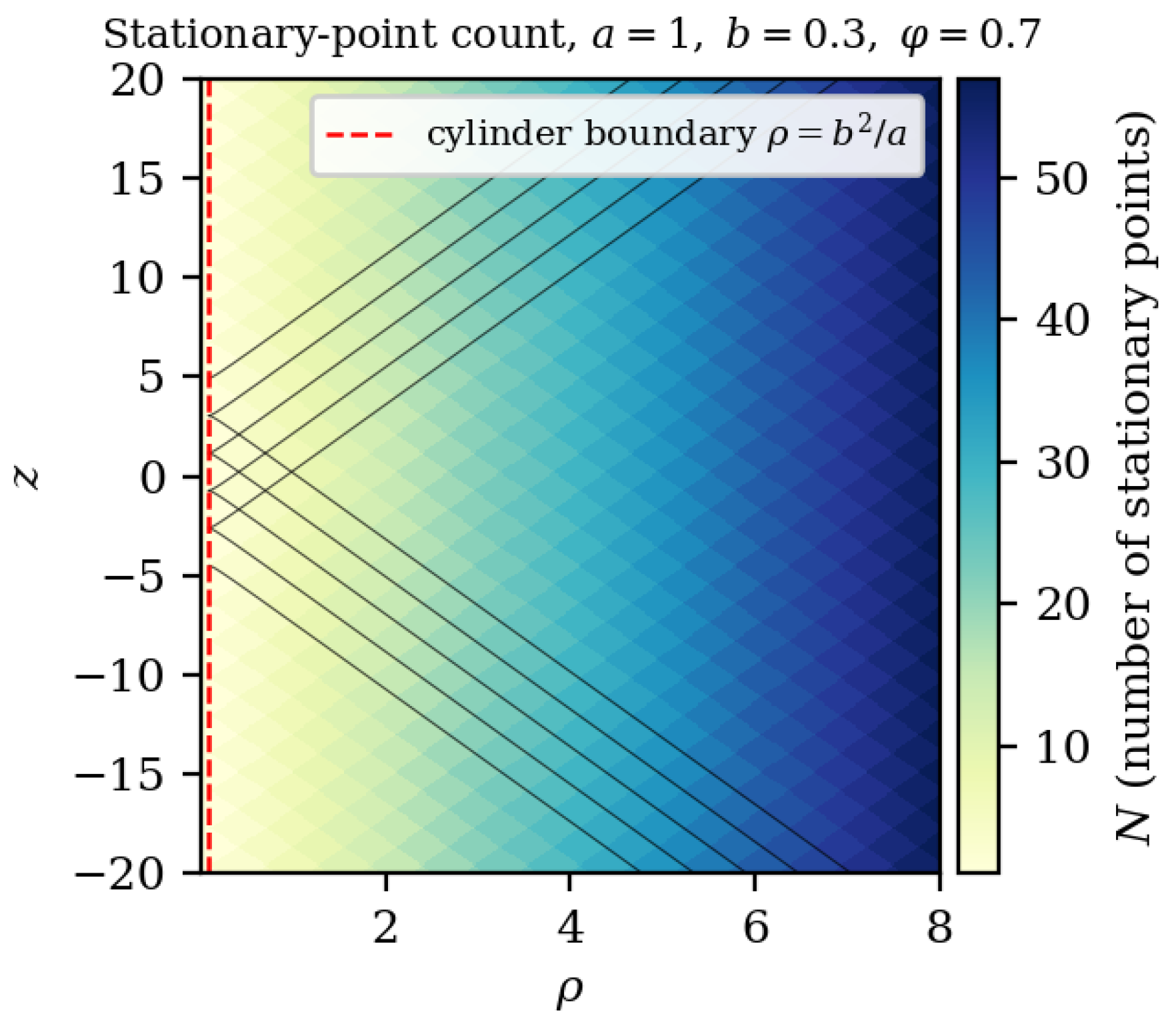
Figure 2.
Universal bifurcation diagram in the plane: the fold lines (black), the Maxwell lines (red dashed), and the cusp points (open circles) on the evolute helix. The color encodes the number N of stationary points; the vertical dotted line is .
Figure 2.
Universal bifurcation diagram in the plane: the fold lines (black), the Maxwell lines (red dashed), and the cusp points (open circles) on the evolute helix. The color encodes the number N of stationary points; the vertical dotted line is .
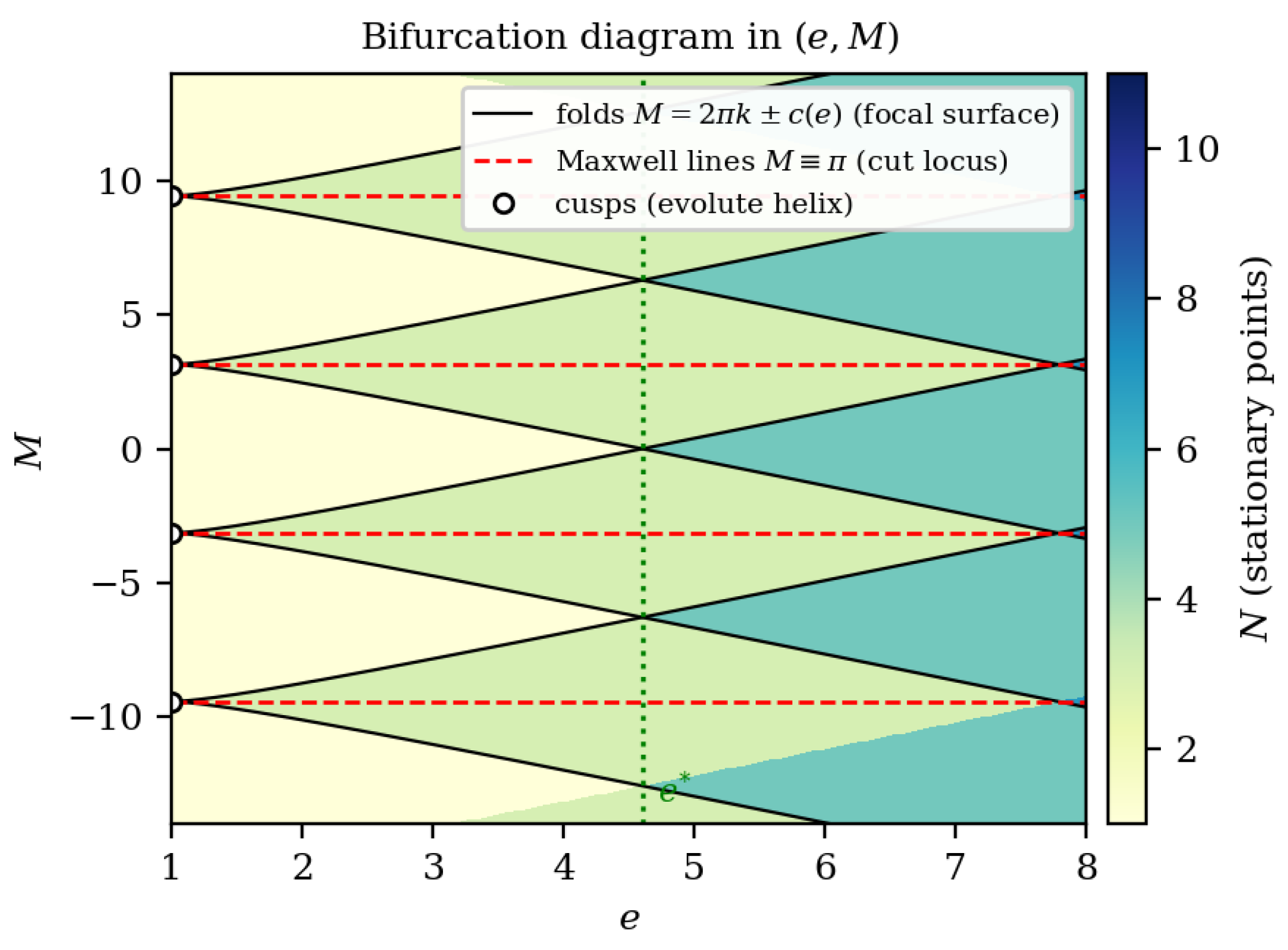
Figure 3.
The helix (blue), its evolute helix (red, the locus of centers of curvature and the cuspidal edge of the focal surface), and the focal surface (orange, the envelope of the normal planes, ruled by the binormal lines through the centers of curvature, two of which are drawn in gray). The focal surface is exactly the set of query points at which the squared distance has a degenerate stationary point.
Figure 3.
The helix (blue), its evolute helix (red, the locus of centers of curvature and the cuspidal edge of the focal surface), and the focal surface (orange, the envelope of the normal planes, ruled by the binormal lines through the centers of curvature, two of which are drawn in gray). The focal surface is exactly the set of query points at which the squared distance has a degenerate stationary point.
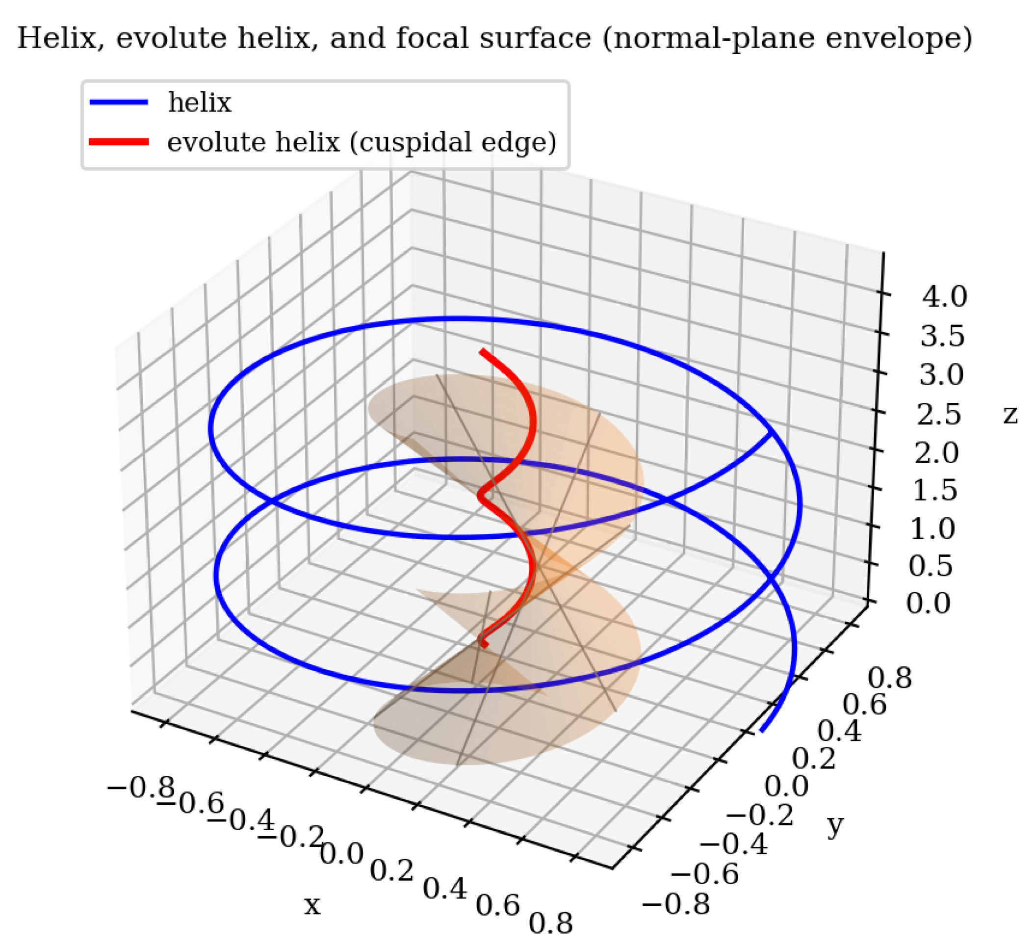
Figure 4.
Solution structure at , . Left: with its seven roots (dots). Right: (using (20)) with the two symmetric global minimizers (green) and the remaining stationary points (red): the exceptional case of Theorem 6(b).
Figure 4.
Solution structure at , . Left: with its seven roots (dots). Right: (using (20)) with the two symmetric global minimizers (green) and the remaining stationary points (red): the exceptional case of Theorem 6(b).
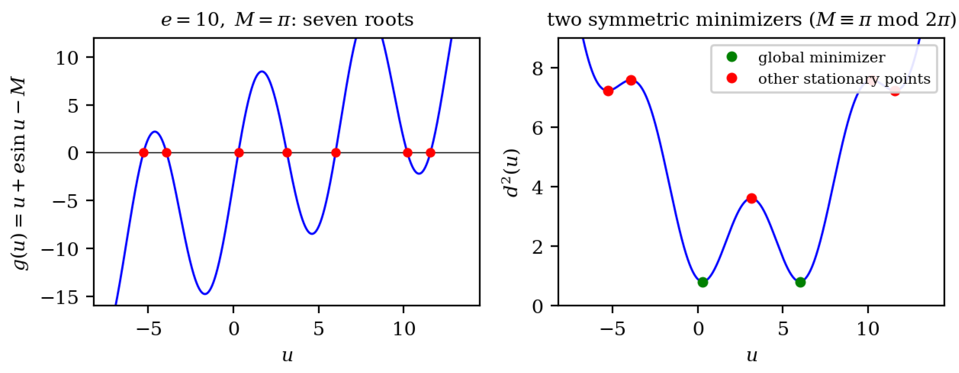
Figure 5.
Quadratic-tangency conditioning at : root separation versus offset from the threshold (dots), with the asymptote , (dashed); vs. .
Figure 5.
Quadratic-tangency conditioning at : root separation versus offset from the threshold (dots), with the asymptote , (dashed); vs. .
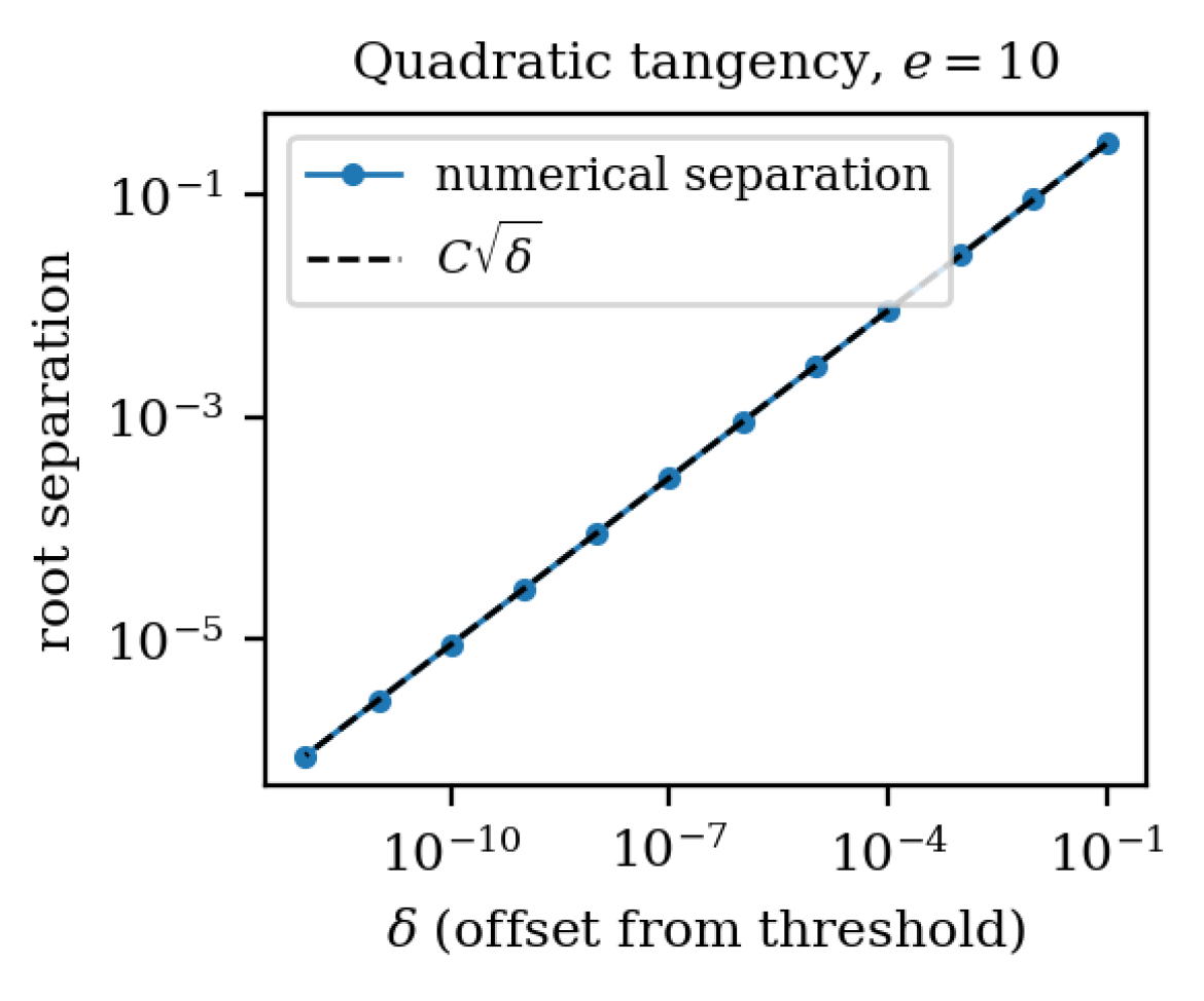
Figure 6.
Conditioning trichotomy: (a) fold, root separation at ; (b) evolute, root shift at , .
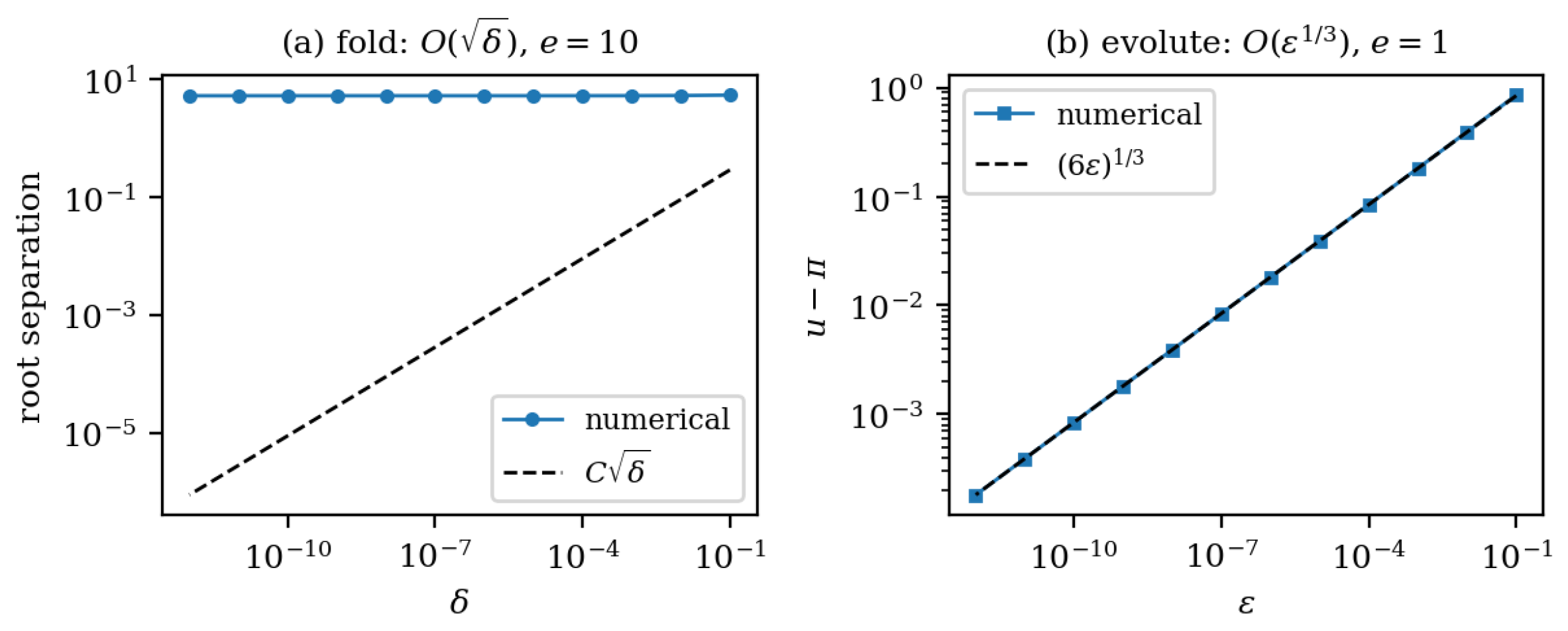

Table 1.
Solver benchmark on random instances, , . “Wrong” means convergence to a stationary point that is not the global minimizer; “failed” means no convergence in 100 iterations. The principal-branch solver returns the global minimizer by construction (Theorem 6).
Table 1.
Solver benchmark on random instances, , . “Wrong” means convergence to a stationary point that is not the global minimizer; “failed” means no convergence in 100 iterations. The principal-branch solver returns the global minimizer by construction (Theorem 6).
| Initialization | wrong (%) | failed (%) | iterations (median/max) |
|---|---|---|---|
| principal branch | 0 | 0 | 6/10 |
| naive (axis projection) | — | ||
| cylinder point [9] | — |
Table 2.
Numerical verification of the theorems (double precision; zero failures throughout). is the closed-form count; is the exact root count by interval isolation.
Table 2.
Numerical verification of the theorems (double precision; zero failures throughout). is the closed-form count; is the exact root count by interval isolation.
| Statement | Specification | Result |
|---|---|---|
| Count law (9) | random , | 0 mismatches |
| Multiplicity law (11) | fold-line + generic | 0 mismatches |
| Cylinder law (Thm. 1) | points, | unique stationary point, all |
| Bifurcation surfaces (Thm. 2) | 600 crossings of (10) | double roots; N jumps |
| Count-region grid | in | 64 crossings; max. loc. err. |
| Focal surface = bifurcation (Thm. 4) | 400 random points of | degenerate root at ; |
| Cuspidal edge (Thm. 4) | 100 points of the evolute helix | , , , |
| Semicubical cusp (15) | ratio | |
| Principal branch (Thm. 6) | random | 0 failures |
| Symmetric case (Thm. 6(b)) | , | exactly two minimizers |
| Cut-locus coalescence (Thm. 5) | ||
| Conditioning bound (17) | random | |
| Hessian bound | random | |
| Fold separation (18) | , | vs. |
| Evolute separation (19) | , | |
| Asymptotics (Prop. 1) | ||
| Two-helix reduction (Thm. 8) | 300 random helix pairs | 0 failures |
| Solver benchmark (Thm. 7) | instances | see Table 1 |
| 1-Lipschitz distance | random pairs | 0 violations |
| (Cor. 1) |
Disclaimer/Publisher’s Note: The statements, opinions and data contained in all publications are solely those of the individual author(s) and contributor(s) and not of MDPI and/or the editor(s). MDPI and/or the editor(s) disclaim responsibility for any injury to people or property resulting from any ideas, methods, instructions or products referred to in the content. |
© 2026 by the authors. Licensee MDPI, Basel, Switzerland. This article is an open access article distributed under the terms and conditions of the Creative Commons Attribution (CC BY) license (http://creativecommons.org/licenses/by/4.0/).
Copyright: This open access article is published under a Creative Commons CC BY 4.0 license, which permit the free download, distribution, and reuse, provided that the author and preprint are cited in any reuse.