Privacy Factor and Relative Fisher Geometry for Parametric Dynamical Systems Under Gaussian Observation Noise

1. Introduction

Imagine a wind farm whose controller continuously adjusts the pitch of each turbine in response to gusts, a fleet of autonomous vehicles exchanging telemetry with a traffic-management server, or a patient wearing a glucose monitor that streams data to a cloud service. In each case a physical system, governed by parameters that may be commercially sensitive, medically private, or operationally confidential, is observed in real time through a noisy channel. The observer—benign or adversarial—accumulates measurements as the system evolves, and may eventually be able to infer not only the current value of those parameters but also the way they change over time. How much can be learned about the parameter trajectory from the observation stream, and how can the system be operated so as to leak as little as possible?

The intuition we will pursue is geometric. Think of the parameter $\theta \left(t\right)$ as drawing a curve in the system’s parameter space; the observations trace a corresponding curve in the data space, smeared by noise. If the two curves nearly coincide with a reference behaviour, the observer learns very little; if they depart from it, every unit of “effort” the parameter spends deviating from the reference shows up, sooner or later, as statistical distinguishability. The natural way to quantify this trade-off is to compare the law of the observations under the true trajectory with their law under a reference: the more divergent the two laws are, the more readily the observer can tell them apart, with a precise asymptotic rate governed by classical results in hypothesis testing [2,11]. Taking the exponential of the negative divergence rate yields a single dimensionless number in $(0,1]$, the privacy factor, which measures the asymptotic probability that the best possible test fails to detect a deviation. Maximising it amounts to operating the system along the parametric trajectory that, for a given budget of variation, is hardest to detect.

This intuitive picture turns out to have a clean mathematical counterpart. The space-time parameter manifold inherits a Fisher metric from the observation channel, and curves in this manifold can be assigned an informational energy whose minimisers, at fixed kinetic budget, solve a variational eigenvalue problem. The first eigenvalue ${\lambda }_1$ of this problem is the intrinsic constant of the system: it sets the optimal leakage rate per unit of variational work, and the associated eigenfunction is the optimal-privacy parametric path. In the linear Gaussian case the problem reduces to a generalised matrix eigenproblem of standard Galerkin type, computable in closed form.

Three lines of work in the privacy literature for dynamical systems are relevant to the present paper. The first is differential privacy for trajectories and control loops, originating in the algorithmic results of Dwork and collaborators [19] and adapted to filtering and time-series releases by Le Ny, Pappas, Cortés and others [20,21]; these guarantees are worst-case and typically achieved by injecting calibrated noise into the released outputs. The second is information-theoretic privacy, where mutual information or KL divergence between sensitive variables and released observations plays the role of leakage measure [22,23]; this strand has focused mainly on memoryless or i.i.d. channels. The third addresses privacy in stochastic processes and stochastic control [24,25,26], often via the Fisher information of the parameter estimator. The framework we propose is closest in spirit to the third strand, in that it works with a Fisher-type metric, but differs from all three in two respects: it treats the noise already present in the observation channel as the privacy resource (no additional noise is injected); and it reduces the problem of finding the optimal parametric path to a single spectral problem whose first eigenvalue plays the role of an intrinsic privacy-efficiency constant.

Section 2 introduces the probabilistic setup, the Kullback–Leibler divergence and the privacy factor. Section 3 develops the relative Fisher metric on the space-time manifold $\widehat{\Theta }=[0,T]\times \Theta$. Section 4 defines the relative informational energy functional, the Rayleigh quotient, and the variational eigenvalue problem that characterises stationary curves. Section 5 specialises to linear Gaussian dynamics, where the bilinear form is explicit, the structural assumptions are verified concretely, and the Galerkin method delivers a finite-dimensional spectral approximation with monotone convergence. Section 6 establishes the asymptotic upper bound on the KL divergence in terms of the energy functional and the resulting lower bound on the privacy factor, together with its connection to the first eigenvalue.

2. Probabilistic Setup, Divergence, and Privacy Factor

Consider a parametric dynamical system

$$\left\{\begin{array}{c}\dot{x}(t,\theta )=f(t,x,\theta )\hfill \\ x\left(0\right)=x_0\hfill \end{array}\right.$$

(1)

where $t\in [0,T]$, $\theta \in \Theta \subset {\mathbb{R}}^q$ is the parameter vector, and f is smooth. An external observer $\mathcal{O}$ who knows (1) and $x_0$ measures the system through the noisy observable

$$y\left(t\right)=h(t,x(t),\theta )+\nu \left(t\right),$$

(2)

where $h:[0,T]\times {\mathbb{R}}^n\times \Theta \to {\mathbb{R}}^m$ is $C^1$ in all arguments and $\nu \left(t\right)$ is a zero-mean Gaussian sensor noise of fixed, time-invariant covariance ${\Sigma }_0\succ 0$, independent across the sampling instants below. Relative to the initial reading,

$$y\left(t\right)-h(0,x_0,\theta )\sim \mathcal{N}\left(\mu (t,x,\theta ),\Sigma \left(t\right)\right),$$

(3)

with

$$\mu (t,x,\theta )=h(t,x\left(t\right),\theta )-h(0,x_0,\theta ),\Sigma \left(t\right)\equiv {\Sigma }_0.$$

(4)

This is the natural model for repeated independent measurements of a fixed-precision instrument.

Suppose that the observer samples (2) uniformly at times

$$t_i=a+i\Delta t,i=1,\dots ,T,\Delta t={\displaystyle \frac{b-a}{T}},$$

(5)

obtaining $Y:=\{y_1,\dots ,y_T\}$ with

$$y_i=\mu (t_i,x(t_i\mid \theta \left(t_i\right)),\theta \left(t_i\right))+w_i,w_i\sim \mathcal{N}(0,{\Sigma }_0),$$

(6)

the noise terms $\left\{w_i\right\}$ are mutually independent. The joint law conditioned on $\theta (·)$ is

$$P_{\theta }^{\left(T\right)}={\displaystyle \underset{i=1}{\overset{T}{⨂}}}\mathcal{N}({\mu }_i,{\Sigma }_i),{\mu }_i:=\mu (t_i,x(t_i\mid \theta \left(t_i\right)),\theta \left(t_i\right)),{\Sigma }_i:=\Sigma \left(t_i\right)={\Sigma }_0.$$

(7)

The object $P_{\theta }^{\left(T\right)}$ represents everything the observer can see: any inference or test is a function of a sample from $P_{\theta }^{\left(T\right)}$.

We now introduce an instrument for comparing different distributions.

Definition 1

([1,2]). Let $P,Q$ be probability laws on $(\mathcal{Y},\mathcal{B})$ with $P\ll Q$. The Kullback–Leibler divergence is

$$D_{KL}(P\parallel Q):={\int }_{\mathcal{Y}}\log {\displaystyle \frac{dP}{dQ}}dP\in [0,+\infty ].$$

(8)

Here we recall some basic properties.

Lemma 1.

If $P^{\left(T\right)}={⨂}_{i=1}^T{P}_i$ and $Q^{\left(T\right)}={⨂}_{i=1}^T{Q}_i$ with $P_i\ll Q_i$, then

$$D_{KL}\left(P^{\left(T\right)}\parallel Q^{\left(T\right)}\right)={\displaystyle \sum _{i=1}^T}{D}_{KL}(P_i\parallel Q_i).$$

(9)

Lemma 2.

Let $P=\mathcal{N}({\mu }_1,\Sigma )$ and $Q=\mathcal{N}({\mu }_2,\Sigma )$ with $\Sigma \succ 0$. Then

$$D_{KL}(P\parallel Q)=\frac{1}{2}{({\mu }_1-{\mu }_2)}^{\top }{\Sigma }^{-1}({\mu }_1-{\mu }_2).$$

(10)

Proof. 

Expanding the Gaussian densities gives $\log (p_1/p_2)={({\mu }_1-{\mu }_2)}^{\top }{\Sigma }^{-1}y-\frac{1}{2}({\mu }_1^{\top }{\Sigma }^{-1}{\mu }_1-{\mu }_2^{\top }{\Sigma }^{-1}{\mu }_2)$. Taking expectation under $P=\mathcal{N}({\mu }_1,\Sigma )$ with ${\mathbb{E}}_P\left[y\right]={\mu }_1$ and simplifying gives (10). □

Corollary 1.

For $P^{\left(T\right)}={⨂}_i\mathcal{N}({\mu }_i^P,{\Sigma }_i)$ and $Q^{\left(T\right)}={⨂}_i\mathcal{N}({\mu }_i^Q,{\Sigma }_i)$ with ${\Sigma }_i\succ 0$,

$$D_{KL}\left(P^{\left(T\right)}\parallel Q^{\left(T\right)}\right)=\frac{1}{2}{\displaystyle \sum _{i=1}^T}{({\mu }_i^P-{\mu }_i^Q)}^{\top }{\Sigma }_i^{-1}({\mu }_i^P-{\mu }_i^Q).$$

(11)

Proof. 

Combine Lemmas 1 and 2. □

The total divergence $D_{KL}(P^{\left(T\right)}\parallel Q^{\left(T\right)})$ grows linearly with T and is thus not a resolution-independent privacy measure [2,8]. We normalize and pass to the limit.

Definition 2.

A reference law for the observation process is a sequence of product Gaussian measures

$$Q^{\left(T\right)}={\displaystyle \underset{i=1}{\overset{T}{⨂}}}\mathcal{N}\left({\mu }^q\left(t_i\right),{\Sigma }_i\right),i=1,\dots ,T,$$

(12)

where ${\mu }^q:[0,T]\to {\mathbb{R}}^m$ is a deterministic function of time alone, sharing the noise covariance ${\Sigma }_i$ of $P_{\theta }^{\left(T\right)}$ in (7).

Definition 3

([6,8,12]). The KL rate of P with respect to a reference law Q is

$$\overline{D}(P\parallel Q):=\underset{T\to \infty }{\mathrm{lim\; sup}}{\displaystyle \frac{1}{T}}{D}_{KL}\left(P^{\left(T\right)}\parallel Q^{\left(T\right)}\right).$$

(13)

Definition 4.

The absolute privacy factor of P with respect to a reference law Q is

$${\overline{\Pi }}_{\mathrm{abs}}(P\parallel Q):=\exp \left(-\overline{D}(P\parallel Q)\right)\in (0,1].$$

(14)

Remark 1.

We adopt the lim sup formulation rather than the ordinary limit for two reasons. First, the lim sup exists for every sequence of laws $P^{\left(T\right)},Q^{\left(T\right)}$, so $\overline{D}$ is well-defined without any additional hypothesis. Second, the lim sup is the conservative choice from the privacy perspective: it controls the worst-case exponential rate of optimal hypothesis tests in Stein’s sense [2]. When the limit ${\lim }_{T\to \infty }\frac{1}{T}{D}_{KL}(P^{\left(T\right)}\parallel Q^{\left(T\right)})$ exists, the lim sup in (13) coincides with this limit. All bounds below remain valid for the lim sup.

The factor ${\overline{\Pi }}_{\mathrm{abs}}$ attains its extreme values as follows: ${\overline{\Pi }}_{\mathrm{abs}}=1$ when the KL rate is zero (maximal privacy: the trajectory is statistically indistinguishable from the reference at every frequency), and ${\overline{\Pi }}_{\mathrm{abs}}\to 0$ when $\overline{D}\to +\infty$ (zero privacy).

The exponential form is motivated by Stein’s lemma [11]: for the test $H_0:Q$ vs $H_1:P$, the optimal type-II error at fixed level decays as $e^{-T\overline{D}(P\parallel Q)}$ [12,13]. Thus ${\overline{\Pi }}_{\mathrm{abs}}$ corresponds, up to normalization, to the Bahadur efficiency of the optimal test [15] — the asymptotic probability that the adversary fails to distinguish P from Q.

3. Relative Fisher Metric

Throughout the paper we use t for physical time (the variable of the original dynamical system and of the sampling times $t_i$) and s for the parameter along curves on $\widehat{\Theta }$. When a curve is in graph form (Definition 8) the two coincide, $s=t$. Where no ambiguity arises we tacitly identify the two; otherwise we make the dependence explicit by writing $\gamma \left(s\right)=\left(t\right(s),\theta (s\left)\right)$.

Now we have to go in the geometric details. The parameter space extended to time,

$$\widehat{\Theta }:=[0,T]\times \Theta ,$$

is a differentiable $(q+1)$-dimensional manifold. A generic local coordinate is $\xi =(s,{\theta }^1,\dots ,{\theta }^q)$, with s the temporal component. We use index 0 for the temporal component, indices $1,\dots ,q$ for the parametric ones, and Latin indices $a,b,c$ running over $\{0,1,\dots ,q\}$.

The manifold $\widehat{\Theta }$ inherits the Fisher metric by pullback from the statistical space $\{p_{\xi }=\mathcal{N}(\mu \left(\xi \right),\Sigma \left(s\right))\}$ [3]:

$$g_{ab}\left(\xi \right):={\mathbb{E}}_p\left[\left({\partial }_a\log p\right)\left({\partial }_b\log p\right)\right]={\left({\partial }_a\mu \right)}^{\top }\Sigma {\left(s\right)}^{-1}\left({\partial }_b\mu \right).$$

(15)

Here ${\partial }_a\log p(y;\xi )$ denotes the scalar partial derivative of $\log p$ with respect to the a-th coordinate of $\xi$, so the expectation above is of a product of two scalar functions of y. This metric measures velocity of $\mu \left(\xi \right)$ in the absolute observation space. To adapt it to a fixed reference, we introduce the following.

Definition 5.

Fix a reference q with mean ${\mu }^q:[0,T]\to {\mathbb{R}}^m$ depending only on s. The relative observable is

$$\tilde{\mu }(s,\theta ):=\mu (s,\theta )-{\mu }^q\left(s\right).$$

(16)

Definition 6.

The Fisher metric relative to qon $\widehat{\Theta }$ is

$${\tilde{g}}_{ab}\left(\xi \right):={\left({\partial }_a\tilde{\mu }\right)}^{\top }\Sigma {\left(s\right)}^{-1}\left({\partial }_b\tilde{\mu }\right),a,b=0,1,\dots ,q.$$

(17)

We now collect the basic properties of $\tilde{g}$.

Proposition 1.

The metric $\tilde{g}$ satisfies:

(i) 

Purely parametric components are reference-independent: ${\tilde{g}}_{ij}=g_{ij}$ for all $i,j\in \{1,\dots ,q\}$.

(ii) 

Temporal and mixed components depend on ${\dot{\mu }}^q$:

$${\tilde{g}}_{0j}\left(\xi \right)={({\partial }_0\mu -{\dot{\mu }}^q)}^{\top }{\Sigma }^{-1}\left({\partial }_j\mu \right),{\tilde{g}}_{00}\left(\xi \right)={\parallel {\partial }_0\mu -{\dot{\mu }}^q\parallel }_{{\Sigma }^{-1}}^2.$$

(iii) 

If ${\mu }^q$ is constant, then $\tilde{g}\equiv g$.

(iv) 

When ${\mu }^q\left(s\right)=\mu (s,{\theta }_0)$ (nominal reference), $\tilde{g}$ depends on θ only through $\eta :=\theta -{\theta }_0$.

Proof. (i) Since ${\mu }^q$ depends only on s, ${\partial }_i\tilde{\mu }={\partial }_i\mu$ for $i\ge 1$. (ii) ${\partial }_0\tilde{\mu }={\partial }_0\mu -{\dot{\mu }}^q$; substitute into (17). (iii) If ${\dot{\mu }}^q=0$, all blocks recover g. (iv) When ${\mu }^q\left(s\right)=\mu (s,{\theta }_0)$, the dependence on $\theta$ in ${\partial }_0\tilde{\mu }$ and ${\partial }_j\tilde{\mu }$ occurs exclusively through $\eta =\theta -{\theta }_0$. □

The metric $\tilde{g}$ is the Fisher metric of the statistical space of deviations from the reference. While g measures absolute velocity in the observation space, $\tilde{g}$ measures the velocity of the deviation curve $s\mapsto \tilde{\mu }(s,\theta \left(s\right))$. When ${\mu }^q\left(s\right)=\mu (s,{\theta }_0)$, the metric $\tilde{g}$ is translation-invariant in parameter space (property (iv)), making it structurally simpler than the absolute metric.

4. Informational Energy Functional and Spectral Problem

We now introduce the core of this paper: the variational approach to the privacy problem in the Fisher-metric context.

Definition 7.

For a curve $\gamma :[a,b]\to \widehat{\Theta }$ with $\gamma \left(s\right)=(s,\theta (s\left)\right)$, the Fisher energy is

$$\tilde{E}\left[\gamma \right]:=\frac{1}{2}{\int }_a^b{\tilde{g}}_{ab}\left(\gamma \left(s\right)\right){\dot{\gamma }}^a\left(s\right){\dot{\gamma }}^b\left(s\right)ds.$$

(18)

Setting $\delta \mu \left(s\right):=\mu (s,\theta \left(s\right))-{\mu }^q\left(s\right)$ and $\delta \dot{\mu }:=\frac{d}{ds}\delta \mu$, and using the previous results for the Gaussian case, this becomes

$$\tilde{E}\left[\gamma \right]=\frac{1}{2}{\int }_a^b\delta \dot{\mu }{\left(s\right)}^{\top }\Sigma {\left(s\right)}^{-1}\delta \dot{\mu }\left(s\right)ds,$$

(19)

the integral of the squared velocity of the deviation curve weighted by the inverse covariance [3]. When ${\dot{\mu }}^q\equiv 0$, the classical Fisher–Rao energy is recovered.

Definition 8.

A curve $\gamma :[a,b]\to \widehat{\Theta }$ is a t-section if $t\left(s\right)={\gamma }^0\left(s\right)$ is strictly monotone. It is in graph form if ${\dot{\gamma }}^0=+1$, equivalently if ${\gamma }^0\left(s\right)=s$.

Remark 2.

Compatibility with the endpoints ${\gamma }^0\left(a\right)=a$, ${\gamma }^0\left(b\right)=b$ and strict monotonicity force, after reparametrisation, the graph form ${\gamma }^0\left(s\right)=s$. We therefore identify every admissible t-section with its graph $\gamma \left(s\right)=(s,\theta (s\left)\right)$, $s\in [a,b]$, and write the deviation as $\eta \left(s\right):=\theta \left(s\right)-{\theta }_0$.

Suppose now that $\gamma \left(t\right)={\theta }_0+\eta \left(t\right)$ where ${\theta }_0\in \Theta$ is fixed. We impose $\eta \left(a\right)=0$ and leave $\eta \left(b\right)$ free. The admissible space is

$$\mathcal{V}:=\left\{\eta \in H^1([a,b];{\mathbb{R}}^q):\eta \left(a\right)=0\right\},$$

(20)

a Hilbert space with inner product [17] ${\langle {\eta }_1,{\eta }_2\rangle }_{H^1}={\int }_a^b({\eta }_1^{\top }{\eta }_2+{\dot{\eta }}_1^{\top }{\dot{\eta }}_2)ds$.

We assume henceforth that $\tilde{E}[·]$ restricts to a continuous quadratic form on $\mathcal{V}$, i.e., there exists a bounded symmetric bilinear form $\mathcal{E}:\mathcal{V}\times \mathcal{V}\to \mathbb{R}$ with $\tilde{E}\left[\eta \right]=\frac{1}{2}\mathcal{E}(\eta ,\eta )$. This holds in the linear Gaussian setting (Section 5); see Proposition 3.

Define the Euclidean kinetic energy and its bilinear form:

$$K\left[\eta \right]:=\mathcal{K}(\eta ,\eta ),\mathcal{K}({\eta }_1,{\eta }_2):={\int }_a^b{\dot{\eta }}_1{\left(s\right)}^{\top }{\dot{\eta }}_2\left(s\right)ds.$$

(21)

For $\eta \in \mathcal{V}$, the Poincaré inequality together with the boundary condition $\eta \left(a\right)=0$ gives $K\left[\eta \right]=0\iff \eta \equiv 0$, so K is non-degenerate.

Definition 9.

For each $\eta \in \mathcal{V}\setminus \left\{0\right\}$,

$$\mathcal{R}\left[\eta \right]:={\displaystyle \frac{\tilde{E}\left[\eta \right]}{K\left[\eta \right]}}={\displaystyle \frac{\mathcal{E}(\eta ,\eta )}{2\mathcal{K}(\eta ,\eta )}}.$$

(22)

The quotient $\mathcal{R}\left[\eta \right]$ is the informational leakage rate per unit of Euclidean work. It is scale-invariant: $\mathcal{R}\left[c\eta \right]=\mathcal{R}\left[\eta \right]$ for all $c\ne 0$, so it characterizes the shape of $\eta$, not its amplitude.

Lemma 3.

For every $\eta ,v\in \mathcal{V}$,

$$\begin{array}{cc}\hfill \langle D\tilde{E}\left[\eta \right],v\rangle & =\mathcal{E}(\eta ,v),\hfill \end{array}$$

(23)

$$\begin{array}{cc}\hfill \langle DK\left[\eta \right],v\rangle & =2\mathcal{K}(\eta ,v)=2{\int }_a^b\dot{\eta }{\left(s\right)}^{\top }\dot{v}\left(s\right)ds.\hfill \end{array}$$

(24)

The two bilinear forms $\mathcal{E}$ and $\mathcal{K}$ are distinct objects on $\mathcal{V}\times \mathcal{V}$: $\mathcal{E}$ is the energy form introduced after Definition 7 (explicitly realised, in the linear Gaussian case, by (41)), while $\mathcal{K}$ is the kinetic form (21), i.e. the $L^2$ inner product of the velocities $\dot{\eta }$ and $\dot{v}$.

Proof. 

By quadraticity of $\tilde{E}$: $\frac{d}{dϵ}{|}_{ϵ=0}\frac{1}{2}\mathcal{E}(\eta +ϵv,\eta +ϵv)=\mathcal{E}(\eta ,v)$. Analogously, $K\left[\eta \right]=\mathcal{K}(\eta ,\eta )$ with $\mathcal{K}$ from (21) gives $\frac{d}{dϵ}{|}_{ϵ=0}K[\eta +ϵv]=2\mathcal{K}(\eta ,v)=2{\int }_a^b{\dot{\eta }}^{\top }\dot{v}ds$. □

Lemma 4.

For every $\eta \in \mathcal{V}$ with $K\left[\eta \right]>0$ and every $v\in \mathcal{V}$,

$$\langle D\mathcal{R}\left[\eta \right],v\rangle ={\displaystyle \frac{1}{K\left[\eta \right]}}\left[\mathcal{E}(\eta ,v)-2\mathcal{R}\left[\eta \right]\mathcal{K}(\eta ,v)\right].$$

(25)

Proof. 

Apply the quotient rule to $\mathcal{R}=\tilde{E}/K$ using Lemma 3. □

Theorem 1.

Let ${\eta }_{*}\in \mathcal{V}$ with $K\left[{\eta }_{*}\right]>0$. The following are equivalent:

(i) 

${\eta }_{*}$ is a stationary point of $\mathcal{R}$;

(ii) 

the pair $({\lambda }_{*},{\eta }_{*})$ with ${\lambda }_{*}:=\mathcal{R}\left[{\eta }_{*}\right]$ satisfies

$$\mathcal{E}({\eta }_{*},v)=2{\lambda }_{*}\mathcal{K}({\eta }_{*},v)\forall v\in \mathcal{V}.$$

(26)

Proof.(i)⇒(ii). Setting $\langle D\mathcal{R}\left[{\eta }_{*}\right],v\rangle =0$ in (25) and dividing by $K\left[{\eta }_{*}\right]>0$ gives (26). (ii)⇒(i). Taking $v={\eta }_{*}$ in (26) and dividing by $2K\left[{\eta }_{*}\right]>0$ shows ${\lambda }_{*}=\mathcal{R}\left[{\eta }_{*}\right]$, then (25) gives zero. □

We have thus found that the perturbation of ${\theta }_0$ which is optimal with respect to the Fisher information metric at fixed kinetic budget is a solution of an eigenvalue problem. This motivates the following definition.

Definition 10.

Find pairs $(\lambda ,\eta )\in \mathbb{R}\times (\mathcal{V}\setminus \{0\left\}\right)$ such that

$$\mathcal{E}(\eta ,v)=2\lambda \mathcal{K}(\eta ,v)\forall v\in \mathcal{V}.$$

(27)

In order to effectively achieve a solution we need some basic assumptions on the involved functionals.

Assumption 1.

The bilinear form $\mathcal{E}$ on $\mathcal{V}$ is:

(A1) 

symmetric and bounded: $|\mathcal{E}({\eta }_1,{\eta }_2)|\le C_E\parallel {\eta }_1{\parallel }_{H^1}{\parallel {\eta }_2\parallel }_{H^1}$;

(A2) 

there exist $\alpha >0$, $\beta \in \mathbb{R}$ with $\mathcal{E}(\eta ,\eta )\ge \alpha K\left[\eta \right]+{\beta \parallel \eta \parallel }_{L^2}^2$.

Under Assumption 1, the compact embedding $H^1\hookrightarrow L^2$ (Rellich–Kondrachov [17]) and the spectral theory of symmetric pencils $(\mathcal{E},2\mathcal{K})$ with $\mathcal{K}$ positive definite [9] imply that problem (26) admits a real, discrete spectrum ${\lambda }_1\le {\lambda }_2\le \dots \to +\infty$, with $\mathcal{K}$-orthonormal eigenfunctions $\left\{{\eta }^{\left(k\right)}\right\}$.

Theorem 2

([9,17]). Under Assumption 1, the first eigenvalue ${\lambda }_1$ admits the variational characterization

$${\lambda }_1=\underset{\eta \in \mathcal{V}\setminus \left\{0\right\}}{\inf }\mathcal{R}\left[\eta \right]=\underset{\eta \in \mathcal{V}\setminus \left\{0\right\}}{\inf }{\displaystyle \frac{\tilde{E}\left[\eta \right]}{K\left[\eta \right]}},$$

(28)

attained by every eigenfunction ${\eta }^{\left(1\right)}$ associated to ${\lambda }_1$. For $k\ge 2$,

$${\lambda }_k=\underset{\begin{array}{c}W\subset \mathcal{V}\\ \dim W=k\end{array}}{\inf }\underset{\eta \in W\setminus \left\{0\right\}}{\sup }\mathcal{R}\left[\eta \right]$$

(29)

5. The Linear Gaussian Case

We now specialize all constructions to the linear Gaussian setting, which admits explicit closed-form expressions for the metric, the energy functional, and the Galerkin matrices, and for which Assumption 1 is verified concretely.

Consider the linear parametric system

$$\dot{x}(t,\theta )=A\left(t\right)x(t,\theta )+B\left(t\right)\theta ,x\left(0\right)=x_0,$$

(30)

with $A\in C^2([0,T];{\mathbb{R}}^{n\times n})$, $B\in C^2([0,T];{\mathbb{R}}^{n\times q})$, and the affine observable

$$h(t,x,\theta )=Cx+D,C\in {\mathbb{R}}^{m\times n},D\in {\mathbb{R}}^m.$$

(31)

We take the sensor covariance time-invariant, $\Sigma \left(t\right)\equiv {\Sigma }_0$ with ${\Sigma }_0\succ 0$ (fixed-precision measurements).

By linearity, $x(t,\theta )=\xi \left(t\right)+\mathcal{B}\left(t\right)\theta$ where

$$\dot{\xi }=A\left(t\right)\xi ,\xi \left(0\right)=x_0;\dot{\mathcal{B}}=A\left(t\right)\mathcal{B}+B\left(t\right),\mathcal{B}\left(0\right)=0,$$

(32)

so the observation mean is

$$\mu (t,\theta )=C(\xi \left(t\right)-x_0)+C\mathcal{B}\left(t\right)\theta .$$

(33)

With nominal reference at ${\theta }_0$, the relative observable (16) becomes

$$\tilde{\mu }(s,\theta )=C\mathcal{B}\left(s\right)\eta ,\eta :=\theta -{\theta }_0.$$

(34)

Define

$$\begin{array}{cc}\hfill M& :=C^{\top }{\Sigma }_0^{-1}C\in {\mathbb{R}}^{n\times n},M=M^{\top },M⪰0,\hfill \end{array}$$

(35)

$$\begin{array}{cc}\hfill \mathcal{M}\left(s\right)& :=\mathcal{B}{\left(s\right)}^{\top }M\mathcal{B}\left(s\right),\mathcal{N}\left(s\right):=\mathcal{B}{\left(s\right)}^{\top }M\dot{\mathcal{B}}\left(s\right),\mathcal{P}\left(s\right):=\dot{\mathcal{B}}{\left(s\right)}^{\top }M\dot{\mathcal{B}}\left(s\right).\hfill \end{array}$$

(36)

Here $\mathcal{M}$ and $\mathcal{P}$ are symmetric, while $\mathcal{N}$ is not symmetric in general. The following elementary identity holds.

Lemma 5.

$\dot{\mathcal{M}}\left(s\right)=\mathcal{N}\left(s\right)+\mathcal{N}{\left(s\right)}^{\top }$.

Proof. 

Differentiate $\mathcal{M}={\mathcal{B}}^{\top }M\mathcal{B}$ using the product rule. □

Definition 11.

The model satisfies observational identifiability on $[a,b]$ if $\mathcal{M}\left(s\right)\succ 0$ for all $s\in [a,b]$.

Remark 3.

If $\mathcal{M}\left(s\right)$ is only positive semidefinite—i.e. observational identifiability fails—there exist directions $\eta \in {\mathbb{R}}^q$ with $\mathcal{M}\left(s\right)\eta =0$ for all $s\in [a,b]$, meaning those parameter directions leave the relative observable $\tilde{\mu }(s,\theta )=C\mathcal{B}\left(s\right)\eta$ unchanged. Such directions are perfectly private : they contribute zero to $\tilde{E}$ and therefore to the KL divergence, so ${\lambda }_1=0$ and the privacy-factor bound (63) reduces to the trivial estimate ${\overline{\Pi }}_{\mathrm{abs}}\ge 1$. Moreover, the optimal trajectory is no longer unique. A complete treatment requires decomposing ${\mathbb{R}}^q$ into an observable subspace (on which $\mathcal{M}\left(s\right)$ is positive definite) and a hidden subspace (the kernel of $\mathcal{M}\left(s\right)$), and restricting the spectral problem to the former. We assume observational identifiability throughout and defer the degenerate case to future work.

The first step in specialising the eigenproblem to this case is to identify the elements involved. We begin with $\tilde{g}$.

Proposition 2.

For the linear Gaussian system, the components of $\tilde{g}$ at $(s,\theta )$ are

$$\begin{array}{cc}\hfill {\tilde{g}}_{ij}(s,\theta )& ={\left[\mathcal{M}\left(s\right)\right]}_{ij},\hfill \end{array}$$

(37)

$$\begin{array}{cc}\hfill {\tilde{g}}_{0j}(s,\theta )& ={\left[\mathcal{N}{\left(s\right)}^{\top }\eta \right]}_j,\hfill \end{array}$$

(38)

$$\begin{array}{cc}\hfill {\tilde{g}}_{00}(s,\theta )& ={\eta }^{\top }\mathcal{P}\left(s\right)\eta .\hfill \end{array}$$

(39)

Proof. 

From (34): ${\partial }_i\tilde{\mu }=C\mathcal{B}{\widehat{e}}_i$ and ${\partial }_0\tilde{\mu }=C\dot{\mathcal{B}}\eta$. Substituting into (17) with $\Sigma {\left(s\right)}^{-1}={\Sigma }_0^{-1}$ and $M=C^{\top }{\Sigma }_0^{-1}C$:

$$\begin{array}{cc}\hfill {\tilde{g}}_{ij}& ={\widehat{e}}_i^{\top }{\mathcal{B}}^{\top }M\mathcal{B}{\widehat{e}}_j={\mathcal{M}}_{ij},\hfill \\ \hfill {\tilde{g}}_{0j}& ={\eta }^{\top }{\dot{\mathcal{B}}}^{\top }M\mathcal{B}{\widehat{e}}_j={\left[{\mathcal{N}}^{\top }\eta \right]}_j,\hfill \\ \hfill {\tilde{g}}_{00}& ={\eta }^{\top }{\dot{\mathcal{B}}}^{\top }M\dot{\mathcal{B}}\eta ={\eta }^{\top }\mathcal{P}\eta .\hfill \end{array}$$

□

From this, the energy $\tilde{E}$ follows.

Proposition 3.

Along a t-section $\gamma \left(s\right)=(s,{\theta }_0+\eta \left(s\right))$,

$$\tilde{E}\left[\gamma \right]=\frac{1}{2}{\int }_a^b\left[{\eta }^{\top }\mathcal{P}\left(s\right)\eta +2{\dot{\eta }}^{\top }\mathcal{N}\left(s\right)\eta +{\dot{\eta }}^{\top }\mathcal{M}\left(s\right)\dot{\eta }\right]ds.$$

(40)

Proof. 

With ${\dot{\gamma }}^0=1$, ${\dot{\gamma }}^j={\dot{\eta }}^j$, the integrand ${\tilde{g}}_{ab}{\dot{\gamma }}^a{\dot{\gamma }}^b={\tilde{g}}_{00}+2{\tilde{g}}_{0j}{\dot{\eta }}^j+{\tilde{g}}_{ij}{\dot{\eta }}^i{\dot{\eta }}^j$ becomes, using Proposition 2,

$${\eta }^{\top }\mathcal{P}\eta +2{\eta }^{\top }{\mathcal{N}}^{\top }\dot{\eta }+{\dot{\eta }}^{\top }\mathcal{M}\dot{\eta }.$$

The mixed term is the scalar ${\eta }^{\top }{\mathcal{N}}^{\top }\dot{\eta }={\dot{\eta }}^{\top }\mathcal{N}\eta$, hence the writing in (40). Integrating over $[a,b]$ gives the claim. □

The formula (40) shows that $\tilde{E}$ is a continuous quadratic form on $\mathcal{V}$; the associated symmetric bilinear form is

$$\mathcal{E}({\eta }_1,{\eta }_2):={\int }_a^b\left[{\eta }_1^{\top }\mathcal{P}{\eta }_2+{\dot{\eta }}_1^{\top }\mathcal{N}{\eta }_2+{\eta }_1^{\top }{\mathcal{N}}^{\top }{\dot{\eta }}_2+{\dot{\eta }}_1^{\top }\mathcal{M}{\dot{\eta }}_2\right]ds.$$

(41)

Symmetry of $\mathcal{E}$ is manifest: $\mathcal{M}$ and $\mathcal{P}$ are symmetric, and the mixed terms ${\dot{\eta }}_1^{\top }\mathcal{N}{\eta }_2$ and ${\eta }_1^{\top }{\mathcal{N}}^{\top }{\dot{\eta }}_2$ exchange under ${\eta }_1\leftrightarrow {\eta }_2$. The specialisation ${\eta }_1={\eta }_2=\eta$ recovers (40) via $\mathcal{E}(\eta ,\eta )=2\tilde{E}\left[\eta \right]$.

Proposition 4.

Assume observational identifiability (Definition 11) and $\mathcal{M},\mathcal{N},\mathcal{P}\in C^0\left([a,b]\right)$. Then Assumption 1 holds with explicit constants. Specifically, set

$$\begin{array}{cccc}\hfill m_{*}& :=\underset{s\in [a,b]}{\inf }{\lambda }_{\min }\left(\mathcal{M}\left(s\right)\right)>0,\hfill & \hfill M_{*}& :=\underset{s\in [a,b]}{\sup }\parallel \mathcal{M}\left(s\right)\parallel ,\hfill \\ \hfill N_{*}& :=\underset{s\in [a,b]}{\sup }\parallel \mathcal{N}\left(s\right)\parallel ,\hfill & \hfill P_{*}& :=\underset{s\in [a,b]}{\sup }\parallel \mathcal{P}\left(s\right)\parallel ,\hfill \end{array}$$

all finite by continuity and compactness of $[a,b]$. Then

(A1) 

$\mathcal{E}$ is bounded:

$$|\mathcal{E}({\eta }_1,{\eta }_2)|\le C_E\parallel {\eta }_1{\parallel }_{H^1}{\parallel {\eta }_2\parallel }_{H^1},C_E:=\max (M_{*},P_{*},2N_{*}).$$

(42)

(A2) 

$\mathcal{E}$ is coercive: for every $\epsilon \in (0,1)$,

$$\mathcal{E}(\eta ,\eta )\ge \alpha K\left[\eta \right]+{\beta \parallel \eta \parallel }_{L^2}^2,$$

(43)

with

$$\alpha :=(1-\epsilon )m_{*},\beta :=P_{*}-{\displaystyle \frac{N_{*}^2}{\epsilon m_{*}}}.$$

(44)

The constant α is strictly positive; β can be made arbitrarily close to $P_{*}$ by choosing $\epsilon \to 1^{-}$, at the price of decreasing the coercivity constant α.

Proof.(A1). Each of the four summands in (41) is controlled by Cauchy–Schwarz in $L^2$: $\left|\int {\eta }_1^{\top }\mathcal{P}{\eta }_{2}ds\right|\le P_{*}\parallel {\eta }_1{\parallel }_{L^2}{\parallel {\eta }_2\parallel }_{L^2}$, and analogously for the other three terms with weights $N_{*},N_{*},M_{*}$ on the appropriate $L^2$-norms of ${\eta }_j$ and ${\dot{\eta }}_j$. Summing and using ${\parallel \eta \parallel }_{L^2}\le {\parallel \eta \parallel }_{H^1}$, $\parallel \dot{\eta }{\parallel }_{L^2}\le {\parallel \eta \parallel }_{H^1}$ yields (42).

(A2). By observational identifiability, $\mathcal{M}\left(s\right)⪰m_{*}{I}_q$ on $[a,b]$. Hence

$${\int }_a^b{\dot{\eta }}^{\top }\mathcal{M}\left(s\right)\dot{\eta }ds\ge m_{*}{\int }_a^b{\parallel \dot{\eta }\parallel }^{2}ds=m_{*}K\left[\eta \right].$$

The cross term is controlled by Young’s inequality with parameter $\epsilon \in (0,1)$:

$$2\left|{\int }_a^b{\dot{\eta }}^{\top }\mathcal{N}\left(s\right)\eta ds\right|\le {\displaystyle \frac{N_{*}^2}{\epsilon m_{*}}}{\parallel \eta \parallel }_{L^2}^2+\epsilon m_{*}{\int }_a^b{\parallel \dot{\eta }\parallel }^{2}ds.$$

(Here we used the elementary identity $2|x^{\top }{y|\le \delta \parallel x\parallel }^2+{\delta }^{-1}{\parallel y\parallel }^2$ with $x={\mathcal{N}}^{\top }\eta$, $y=\dot{\eta }$ and $\delta =1/\left(\epsilon m_{*}\right)$, rearranged.) The diagonal $\mathcal{P}$-term contributes $\int {\eta }^{\top }\mathcal{P}\eta ds\ge -P_{*}{\parallel \eta \parallel }_{L^2}^2$ (if $\mathcal{P}$ is not sign-definite; if $\mathcal{P}⪰0$ the bound becomes $+P_{*}$, which only improves (43)). Collecting,

$$\mathcal{E}(\eta ,\eta )\ge (1-\epsilon )m_{*}K\left[\eta \right]-\left({\displaystyle \frac{N_{*}^2}{\epsilon m_{*}}}-P_{*}\right){\parallel \eta \parallel }_{L^2}^2,$$

which is (43) with $\alpha ,\beta$ as in (44). □

Remark 4.

Even when β in (44) is negative, the bound (A2) of Assumption 1 only requires $\alpha >0$, and the Poincaré-type inequality $K\left[\eta \right]\ge C_P{\parallel \eta \parallel }_{L^2}^2$ for $\eta \in \mathcal{V}$ (with $C_P={\pi }^2/\left[4{(b-a)}^2\right]$, from the boundary condition $\eta \left(a\right)=0$ [17]) allows the $L^2$-term to be absorbed into $K\left[\eta \right]$ at the cost of replacing α by $\alpha -\left|\beta \right|/C_P$, which remains positive provided $\left|\beta \right|<\alpha C_P$. This is automatic for sufficiently small ε or whenever the observation window $b-a$ is short enough. In either case the net coercivity constant $\alpha -\left|\beta \right|/C_P$ is strictly positive, so $\mathcal{E}$ is coercive relative to $K[·]$ on $\mathcal{V}$, and the spectral theory of Section 4 applies without modification.

We now have all the ingredients to solve the problem via the Galerkin method. The Galerkin method [9,10] discretizes (26) in a finite-dimensional subspace ${\mathcal{V}}_N\subset \mathcal{V}$. Choose the adapted sine basis satisfying ${\varphi }_{j,\alpha }\left(a\right)=0$:

$${\varphi }_{j,\alpha }\left(s\right):=\sin \left({\displaystyle \frac{(2j-1)\pi }{2(b-a)}}(s-a)\right){\widehat{e}}_{\alpha },j=1,2,\dots ,\alpha =1,\dots ,q,$$

(45)

Remark 5.

The basis (45) satisfies two boundary conditions consistent with the variational problem. By construction, ${\varphi }_{j,\alpha }\left(a\right)=0$ (Dirichlet condition, required by $\mathcal{V}$). For the natural condition at $s=b$, note that with ${\omega }_j:=(2j-1)\pi /\left[2(b-a)\right]$,

$${\varphi }_{j,\alpha }^{\prime }\left(b\right)={\omega }_j\cos \left({\omega }_j(b-a)\right){\widehat{e}}_{\alpha }={\omega }_j\cos \left({\displaystyle \frac{(2j-1)\pi }{2}}\right){\widehat{e}}_{\alpha }=0,$$

(46)

since $\cos \left(\right(2j-1)\pi /2)=0$ for every integer $j\ge 1$. Consequently ${\dot{\eta }}_N\left(b\right)=0$ for every ${\eta }_N\in {\mathcal{V}}_N$, which is consistent. A basis with ${\varphi }_{j,\alpha }\left(b\right)=0$ (full Dirichlet at b) would not respect this condition and would reduce the convergence rate.

and set ${\mathcal{V}}_N:=\mathrm{span}\{{\varphi }_1,\dots ,{\varphi }_N\}$. The Galerkin ansatz is

$${\eta }_N\left(s\right)={\displaystyle \sum _{j=1}^N}{c}_j{\varphi }_j\left(s\right),\mathbf{c}:={(c_1,\dots ,c_N)}^{\top }.$$

(47)

Define the symmetric matrices

$${\left[{\mathbf{M}}_E\right]}_{ij}:=\mathcal{E}({\varphi }_i,{\varphi }_j),{\left[{\mathbf{M}}_K\right]}_{ij}:=2\mathcal{K}({\varphi }_i,{\varphi }_j).$$

(48)

Proposition 5.

Restricting (26) to ${\mathcal{V}}_N$ is equivalent to

$${\mathbf{M}}_E\mathbf{c}=\lambda {\mathbf{M}}_K\mathbf{c},\mathbf{c}\in {\mathbb{R}}^N\setminus \left\{0\right\}.$$

(49)

This has N real eigenvalues ${\lambda }_1^{\left(N\right)}\le \dots \le {\lambda }_N^{\left(N\right)}$ with $\mathcal{K}$-orthonormal eigenvectors.

Proof. 

Substitute (47) into (26) with $v={\varphi }_i$: ${\sum }_j{c}_j\mathcal{E}({\varphi }_j,{\varphi }_i)=\lambda {\sum }_j{c}_j·2\mathcal{K}({\varphi }_j,{\varphi }_i)$, i.e., ${\mathbf{M}}_E\mathbf{c}=\lambda {\mathbf{M}}_K\mathbf{c}$. Symmetry and positive definiteness of ${\mathbf{M}}_K$ give a real spectrum. □

Setting ${\omega }_j:={\displaystyle \frac{(2j-1)\pi }{2(b-a)}}$ and ${\psi }_j\left(s\right):=\sin \left({\omega }_j(s-a)\right)$:

Proposition 6.

In the sine basis (45),

$${\left[{\mathbf{M}}_K\right]}_{(j,\alpha ),(k,\beta )}=(b-a){\omega }_j^2{\delta }_{jk}{\delta }_{\alpha \beta },$$

(50)

so ${\mathbf{M}}_K$ is diagonal. The stiffness matrix ${\mathbf{M}}_E$ has entries

$$\begin{array}{cc}\hfill {\left[{\mathbf{M}}_E\right]}_{(j,\alpha ),(k,\beta )}& ={\int }_a^b\left[{\psi }_j{\psi }_k{\mathcal{P}}_{\alpha \beta }+{\omega }_j{\psi }_j^{\prime }{\psi }_k{\mathcal{N}}_{\alpha \beta }+{\omega }_k{\psi }_j{\psi }_k^{\prime }{\mathcal{N}}_{\beta \alpha }+{\omega }_j{\omega }_k{\psi }_j^{\prime }{\psi }_k^{\prime }{\mathcal{M}}_{\alpha \beta }\right]ds,\hfill \end{array}$$

(51)

where ${\psi }_j^{\prime }\left(s\right)=\cos \left({\omega }_j(s-a)\right)$.

Proof. 

Diagonality of ${\mathbf{M}}_K$ follows from ${\int }_a^b\cos \left({\omega }_j(s-a)\right)\cos \left({\omega }_k(s-a)\right)ds=\frac{b-a}{2}{\delta }_{jk}$ and the factor 2 in (48). The formula for ${\mathbf{M}}_E$ follows from substituting ${\varphi }_{j,\alpha }$, ${\varphi }_{k,\beta }$ into (41). □

Diagonality of ${\mathbf{M}}_K$ reduces the generalized problem to the standard one

$$\left({\mathbf{M}}_K^{-1/2}{\mathbf{M}}_E{\mathbf{M}}_K^{-1/2}\right)\tilde{\mathbf{c}}=\lambda \tilde{\mathbf{c}}.$$

The integrals in (51) are computed via Gauss–Legendre quadrature; the dominant cost is $O\left(J^2{q}^2{N}_{\mathrm{quad}}\right)$ to assemble ${\mathbf{M}}_E$ and $O\left({\left(Jq\right)}^3\right)$ to diagonalize.

We have thus reduced the functional eigenproblem to a matrix eigenproblem via a Galerkin approximation. This approximation converges in an appropriate sense, so we can truncate the expansion after a certain N in order to achieve a satisfactory approximation.

Theorem 3

([9,10]). Under observational identifiability, for each fixed k and $N\ge k$:

(i) 

${\lambda }_k\le {\lambda }_k^{(N+1)}\le {\lambda }_k^{\left(N\right)}$ (monotone from above);

(ii) 

${\lambda }_k^{\left(N\right)}\to {\lambda }_k$ as $N\to \infty$;

(iii) 

if ${\eta }^{\left(k\right)}$ is simple, then ${\eta }_N^{\left(k\right)}\to {\eta }^{\left(k\right)}$ in $\mathcal{V}$.

For the sine basis (45), the error ${\lambda }_k^{\left(N\right)}-{\lambda }_k$ decays as $O\left(N^{-2r}\right)$ with r the Sobolev regularity of ${\eta }^{\left(k\right)}$ [10]. When $\mathcal{M},\mathcal{N},\mathcal{P}\in C^{\infty }$, the decay is exponential in N.

Corollary 2.

Let ${\eta }^{\left(k\right)}$ be an eigenfunction with $K\left[{\eta }^{\left(k\right)}\right]=1$. For every $c\in \mathbb{R}$,

$$K\left[c{\eta }^{\left(k\right)}\right]=c^2,\tilde{E}\left[c{\eta }^{\left(k\right)}\right]={\lambda }_k{c}^2.$$

(52)

Proof. 

Quadraticity of K and $\tilde{E}$, together with $\tilde{E}\left[{\eta }^{\left(k\right)}\right]={\lambda }_{k}K\left[{\eta }^{\left(k\right)}\right]={\lambda }_k$. □

Corollary 3.

Among all t-sections with $K\left[\gamma \right]=K_0$ and $\theta \left(a\right)={\theta }_0$, the curve $\eta =\sqrt{K_0}{\eta }^{\left(1\right)}$ uniquely minimizes $\tilde{E}$:

$$\underset{\eta \in \mathcal{V}:K\left[\eta \right]=K_0}{\min }\tilde{E}\left[\eta \right]={\lambda }_1{K}_0.$$

(53)

Proof. 

By Theorem 2, $\tilde{E}\left[\eta \right]\ge {\lambda }_{1}K\left[\eta \right]={\lambda }_1{K}_0$ for all admissible $\eta$, with equality iff $\eta \propto {\eta }^{\left(1\right)}$. □

Every $\eta \in \mathcal{V}$ decomposes as $\eta ={\sum }_k{c}_k{\eta }^{\left(k\right)}$ with $\mathcal{K}$-orthonormal eigenfunctions, giving

$$K\left[\eta \right]=\sum _k{c}_k^2,\tilde{E}\left[\eta \right]=\sum _k{\lambda }_k{c}_k^2.$$

(54)

Minimizing $\tilde{E}$ at fixed K concentrates all weight on ${\eta }^{\left(1\right)}$. Modes $k\ge 2$ (with ${\lambda }_k>{\lambda }_1$) become relevant only when additional constraints (waypoints, forbidden parametric regions) prevent using ${\eta }^{\left(1\right)}$ alone.

6. Privacy Factor Bound and Connection with the First Eigenvalue

We establish that the informational energy $\tilde{E}\left[\gamma \right]$ controls ${\overline{\Pi }}_{\mathrm{abs}}$ through an explicit asymptotic bound, and connect this bound to the spectral structure via the Rayleigh principle.

We work under the following regularity hypotheses:

(R1)

$h\in C^1([0,T]\times {\mathbb{R}}^n\times \Theta ;{\mathbb{R}}^m)$;

(R2)

$f\in C^1([0,T]\times {\mathbb{R}}^n\times \Theta ;{\mathbb{R}}^n)$;

(R3)

$\theta \in C^1([a,b];\Theta )$;

(R4)

$\Sigma \left(t\right)\equiv {\Sigma }_0\succ 0$ (constant, time-invariant sensor covariance).

Lemma 6.

Under (R1)–(R3), with $\delta \mu \left(s\right):=\mu (s,\theta \left(s\right))-{\mu }^q\left(s\right)$,

$$\delta \mu \left(t_i\right)=\delta \mu \left(a\right)+{\int }_a^{t_i}\delta \dot{\mu }\left(s\right)ds,i=1,\dots ,T.$$

(55)

Lemma 7.

For continuous $v:[a,t_i]\to {\mathbb{R}}^m$ and $A\succ 0$,

$${\left({\int }_a^{t_i}vds\right)}^{\top }A\left({\int }_a^{t_i}vds\right)\le (t_i-a){\int }_a^{t_i}{v}^{\top }Avds.$$

(56)

Proof. 

Apply Jensen’s inequality [18] to the convex quadratic $\varphi \left(v\right)=v^{\top }Av$ under the uniform measure on $[a,t_i]$, then multiply by ${(t_i-a)}^2$. □

Proposition 7.

Under (R1)–(R4), for every t-section γ and every i,

$$\delta \mu {\left(t_i\right)}^{\top }{\Sigma }_0^{-1}\delta \mu \left(t_i\right)\le 2{\parallel \delta \mu \left(a\right)\parallel }_{{\Sigma }_0^{-1}}^2+2(t_i-a){\int }_a^{t_i}{\tilde{g}}_{ab}\left(\gamma \right){\dot{\gamma }}^a{\dot{\gamma }}^{b}ds.$$

(57)

Proof. 

Apply ${\parallel u+v\parallel }_A^2\le {2\parallel u\parallel }_A^2+2{\parallel v\parallel }_A^2$ to (55) with $A={\Sigma }_0^{-1}$, then Lemma 7 with $A={\Sigma }_0^{-1}$ and $v=\delta \dot{\mu }$. Since $\Sigma \left(s\right)\equiv {\Sigma }_0$, the weight ${\Sigma }_i^{-1}$ coincides with $\Sigma {\left(s\right)}^{-1}$ for every s, so the inequality is exact with no remainder. □

Lemma 8.

For the uniform sampling (5) with $k\left(s\right):=\min \{i:t_i\ge s\}$,

$$\Delta t\sum _{i\ge k\left(s\right)}(t_i-a)=\frac{1}{2}\left[{(b-a)}^2-{(s-a)}^2\right]+O(\Delta t).$$

(58)

Proof. 

Set $j=i-k\left(s\right)+1$ and use ${\sum }_{j=1}^{N}j=N(N+1)/2$ with $k\left(s\right)\Delta t\to s-a$ and $T\Delta t=b-a$. □

Theorem 4.

Under (R1)–(R4) and the boundary condition $\delta \mu \left(a\right)=0$ (equivalently $\theta \left(a\right)={\theta }_0$ when ${\mu }^q\left(s\right)=\mu (s,{\theta }_0)$), for every t-section γ and every sufficiently small $\Delta t=(b-a)/T$,

$$D_{KL}\left(P_{\gamma }^{\left(T\right)}\parallel Q^{\left(T\right)}\right)\le {\displaystyle \frac{{(b-a)}^2}{2\Delta t}}\tilde{E}\left[\gamma \right]+R(\Delta t),$$

(59)

where the remainder $R(\Delta t)$ is uniformly bounded as $\Delta t\to 0$: $\left|R\right(\Delta t\left)\right|\le C(\gamma ,\Sigma ,b-a)$, with C depending only on the trajectory γ, the noise covariance Σ and the window length $b-a$. Consequently, for the KL rate,

$$\overline{D}(P_{\gamma }\parallel Q):=\underset{T\to \infty }{\mathrm{lim\; sup}}{\displaystyle \frac{1}{T}}{D}_{KL}(P_{\gamma }^{\left(T\right)}\parallel Q^{\left(T\right)})\le \frac{1}{2}(b-a)\tilde{E}\left[\gamma \right].$$

(60)

Proof. 

By Corollary 1 and Proposition 7, summing the pointwise bound over $i=1,\dots ,T$,

$$2D_{KL}(P_{\gamma }^{\left(T\right)}\parallel Q^{\left(T\right)})\le 2{\displaystyle \sum _{i=1}^T}{\parallel \delta \mu \left(a\right)\parallel }_{{\Sigma }_0^{-1}}^2+2{\displaystyle \sum _{i=1}^T}(t_i-a){\int }_a^{t_i}{\tilde{g}}_{ab}{\dot{\gamma }}^a{\dot{\gamma }}^{b}ds.$$

(61)

First term. Under the standing boundary condition $\delta \mu \left(a\right)=0$ the first sum vanishes identically. (If dropped, it would contribute ${T\parallel \delta \mu \left(a\right)\parallel }_{{\Sigma }_0^{-1}}^2=O\left(T\right)$, hence a nonzero constant to the rate after division by T; under $\delta \mu \left(a\right)=0$ it disappears.)

Main term. Exchange integration and summation:

$${\displaystyle \sum _{i=1}^T}(t_i-a){\int }_a^{t_i}{\tilde{g}}_{ab}{\dot{\gamma }}^a{\dot{\gamma }}^{b}ds={\int }_a^b{\tilde{g}}_{ab}{\dot{\gamma }}^a{\dot{\gamma }}^b{W}_T\left(s\right)ds,W_T\left(s\right):=\sum _{i\ge k\left(s\right)}(t_i-a).$$

By Lemma 8, $\Delta t{W}_T\left(s\right)=\frac{1}{2}[{(b-a)}^2-{(s-a)}^2]+r_T\left(s\right)$ with $|r_T\left(s\right)|\le c\Delta t$ uniformly in $s\in [a,b]$. Therefore

$$\begin{array}{cc}\hfill \sum _i(t_i-a){\int }_a^{t_i}{\tilde{g}}_{ab}{\dot{\gamma }}^a{\dot{\gamma }}^{b}ds& ={\displaystyle \frac{1}{\Delta t}}{\int }_a^b{\tilde{g}}_{ab}{\dot{\gamma }}^a{\dot{\gamma }}^b·\frac{1}{2}[{(b-a)}^2-{(s-a)}^2]ds+R_1(\Delta t)\hfill \\ \hfill & \le {\displaystyle \frac{{(b-a)}^2}{2\Delta t}}{\int }_a^b{\tilde{g}}_{ab}{\dot{\gamma }}^a{\dot{\gamma }}^{b}ds+R_1(\Delta t),\hfill \end{array}$$

where the inequality uses ${(s-a)}^2\ge 0$, and the absolute value of $R_1$ is bounded by $c{\int }_a^b{\tilde{g}}_{ab}{\dot{\gamma }}^a{\dot{\gamma }}^{b}ds=2c\tilde{E}\left[\gamma \right]$, hence again constant in $\Delta t$.

Dividing the resulting inequality by 2 produces (59) with $R(\Delta t)=R_1(\Delta t)$ uniformly bounded as $\Delta t\to 0$. Dividing instead by $T=(b-a)/\Delta t$ gives, for every finite T,

$$\frac{1}{T}{D}_{KL}\left(P_{\gamma }^{\left(T\right)}\parallel Q^{\left(T\right)}\right)\le \frac{1}{2}(b-a)\tilde{E}\left[\gamma \right]+\frac{1}{T}R(\Delta t)=\frac{1}{2}(b-a)\tilde{E}\left[\gamma \right]+o\left(1\right),T\to \infty ,$$

since $R(\Delta t)$ is bounded and $1/T\to 0$. Taking ${\mathrm{lim\; sup}}_{T\to \infty }$ on both sides yields (60). □

Corollary 4.

Under (R1)–(R4),

$${\overline{\Pi }}_{\mathrm{abs}}(P_{\gamma }\parallel Q)\ge \exp \left(-\frac{1}{2}(b-a)\tilde{E}\left[\gamma \right]\right).$$

(62)

Corollary 5.

For every t-section γ with $\eta =\theta -{\theta }_0\in \mathcal{V}$,

$${\overline{\Pi }}_{\mathrm{abs}}(P_{\gamma }\parallel Q)\ge \exp \left(-\frac{1}{2}(b-a){\lambda }_{1}K\left[\gamma \right]\right),$$

(63)

with equality in the Rayleigh principle achieved by $\eta =\sqrt{K\left[\gamma \right]}{\eta }^{\left(1\right)}$. The eigenvalue ${\lambda }_1$ is approximated from above by ${\lambda }_1^{\left(N\right)}$ of the Galerkin problem (49) (Theorem 3).

Proof. 

Corollary 3 gives $\tilde{E}\left[\gamma \right]\ge {\lambda }_{1}K\left[\gamma \right]$. Substituting into (62) yields (63). □

The bound (63) establishes a fundamental privacy-efficiency trade-off: for any parametric budget $K_0=K\left[\gamma \right]$, the optimal curve $\sqrt{K_0}{\eta }^{\left(1\right)}$ has privacy decaying as $\exp (-\frac{1}{2}(b-a){\lambda }_1{K}_0)$. The first eigenvalue ${\lambda }_1$ is the intrinsic constant of the system governing this trade-off, depending only on $\mathcal{M}$, $\mathcal{N}$, $\mathcal{P}$ (dynamics and observable) and the interval $[a,b]$ [3,16].

Theorem 5.

For the linear Gaussian system with nominal reference $Q^{\left(T\right)}={⨂}_i\mathcal{N}(\mu (t_i,{\theta }_0),{\Sigma }_i)$,

$$D_{KL}(P_{\gamma }^{\left(T\right)}\parallel Q^{\left(T\right)})=\frac{1}{2}{\displaystyle \sum _{i=1}^T}\eta {\left(t_i\right)}^{\top }\mathcal{M}\left(t_i\right)\eta \left(t_i\right),\eta \left(t_i\right)=\theta \left(t_i\right)-{\theta }_0.$$

(64)

Proof. 

By Corollary 1, $\mu (t_i,\theta \left(t_i\right))-\mu (t_i,{\theta }_0)=C\mathcal{B}\left(t_i\right)\eta \left(t_i\right)$ by (33). Using ${\Sigma }_i^{-1}={\Sigma }_0^{-1}$ and $M=C^{\top }{\Sigma }_0^{-1}C$ gives each term as ${\eta }^{\top }\mathcal{M}\eta$, yielding (64). □

The formula (64) is an identity and not a bound. Along the scaled eigenfunction ${\gamma }_k\left(s\right):=(s,{\theta }_0+c{\eta }^{\left(k\right)}\left(s\right))$, the KL sum is a Riemann sum converging, as $\Delta t\to 0$, to

$$\Delta t{\displaystyle \sum _{i=1}^T}\frac{1}{2}{c}^2{\eta }^{\left(k\right)}{\left(t_i\right)}^{\top }\mathcal{M}\left(t_i\right){\eta }^{\left(k\right)}\left(t_i\right)\underset{\Delta t\to 0}{\to }\frac{c^2}{2}{\int }_a^b{\eta }^{\left(k\right)}{\left(s\right)}^{\top }\mathcal{M}\left(s\right){\eta }^{\left(k\right)}\left(s\right)ds=:I_k{c}^2,$$

(65)

so that

$$D_{KL}(P_{{\gamma }_k}^{\left(T\right)}\parallel Q^{\left(T\right)})=\frac{c^2{I}_k}{\Delta t}+o(1/\Delta t),\Delta t\to 0.$$

(66)

The bound of Theorem 4 predicts $D_{KL}\le \frac{{(b-a)}^2}{2\Delta t}{\lambda }_k{c}^2+O\left(1\right)$, so the asymptotic gap ratio between the exact divergence and the bound along the k-th eigenmode is

$${\tau }_k^{\infty }:=\underset{T\to \infty }{\lim }{\displaystyle \frac{D_{KL}(P_{{\gamma }_k}^{\left(T\right)}\parallel Q^{\left(T\right)})}{\frac{{(b-a)}^2}{2\Delta t}{\lambda }_k{c}^2}}={\displaystyle \frac{2I_k}{{(b-a)}^2{\lambda }_k}}\in (0,1].$$

(67)

The upper bound ${\tau }_k^{\infty }\le 1$ follows from the Cauchy–Schwarz and Jensen steps used in Theorem 4; equality holds only when those inequalities are saturated, which in general fails along eigenfunctions. The numerical value of ${\tau }_k^{\infty }$ thus quantifies how tight the privacy-factor bound (63) is on the k-th optimal-privacy trajectory of the system.

7. Numerical Results

We instantiate the linear Gaussian framework of Section 5 with the following very easy choices. The state matrix

$$A=\left(\begin{array}{cc}0& 1\\ -1& 0\end{array}\right)$$

(68)

has purely imaginary eigenvalues $\pm \mathrm{i}$. The remaining parameters are

$$B=\left(\begin{array}{cc}1.0& 0.5\\ 0.3& 1.0\end{array}\right),C=\left(\begin{array}{cc}1.0& 0.5\\ 0.2& 0.8\end{array}\right),\Sigma \left(t\right)\equiv {\Sigma }_0=\mathrm{diag}({\sigma }_1^2,{\sigma }_2^2),$$

(69)

with $n=q=m=2$, ${\sigma }_1=0.5$, ${\sigma }_2=1.2$, $x_0={(1,0)}^{\top }$, ${\theta }_0={(0.3,-0.2)}^{\top }$, and observation window $[a,b]=[0.5,10]$. The bivariate observation ($m=2$) with anisotropic noise (${\sigma }_2>{\sigma }_1$) breaks the symmetry between the two parameter components in the Fisher weight $M=C^{\top }{\Sigma }_0^{-1}C\in {\mathbb{R}}^{2\times 2}$, yielding a richer spectral structure than the scalar case. The five qualitative displays (Figure 1, Figure 2, Figure 3 and Figure 4) use a Galerkin space of dimension $N=Jq=4\times 2=8$, sufficient to resolve the geometric features of the lowest modes. All five displayed modes are scaled to kinetic budget $K_0=K\left[{\eta }^{\left(k\right)}\right]=1$.

Figure 1 collects the state-space picture. The left block shows $x_1\left(t\right)$ and $x_2\left(t\right)$ for the nominal trajectory $\theta \equiv {\theta }_0$ (solid black) together with the five mode-optimal perturbations ${\theta }^{\left(k\right)}\left(t\right)={\theta }_0+{\eta }^{\left(k\right)}\left(t\right)$ (dashed). The framing phase-plane panels confirm the center structure: the nominal orbit is a closed circle, while each mode-optimal path deforms it in a pattern determined by the shape of ${\eta }^{\left(k\right)}$. Lower modes ($k=1,2$) produce wider, smoother deformations; higher modes introduce faster oscillations that keep the trajectory close to the nominal.

Figure 1. State trajectories under mode-optimal parameter paths ${\theta }^{\left(k\right)}\left(t\right)={\theta }_0+{\eta }^{\left(k\right)}\left(t\right)$, all scaled to $K_0=1$. Left block: time series $x_1\left(t\right)$ (top) and $x_2\left(t\right)$ (bottom); nominal in solid black, modes $k=1,\dots ,5$ in dashed colour. Framing panels: phase plane $(x_1,x_2)$ per mode vs. nominal; circles mark $t=a$, triangles $t=b$.

Figure 1. State trajectories under mode-optimal parameter paths ${\theta }^{\left(k\right)}\left(t\right)={\theta }_0+{\eta }^{\left(k\right)}\left(t\right)$, all scaled to $K_0=1$. Left block: time series $x_1\left(t\right)$ (top) and $x_2\left(t\right)$ (bottom); nominal in solid black, modes $k=1,\dots ,5$ in dashed colour. Framing panels: phase plane $(x_1,x_2)$ per mode vs. nominal; circles mark $t=a$, triangles $t=b$.

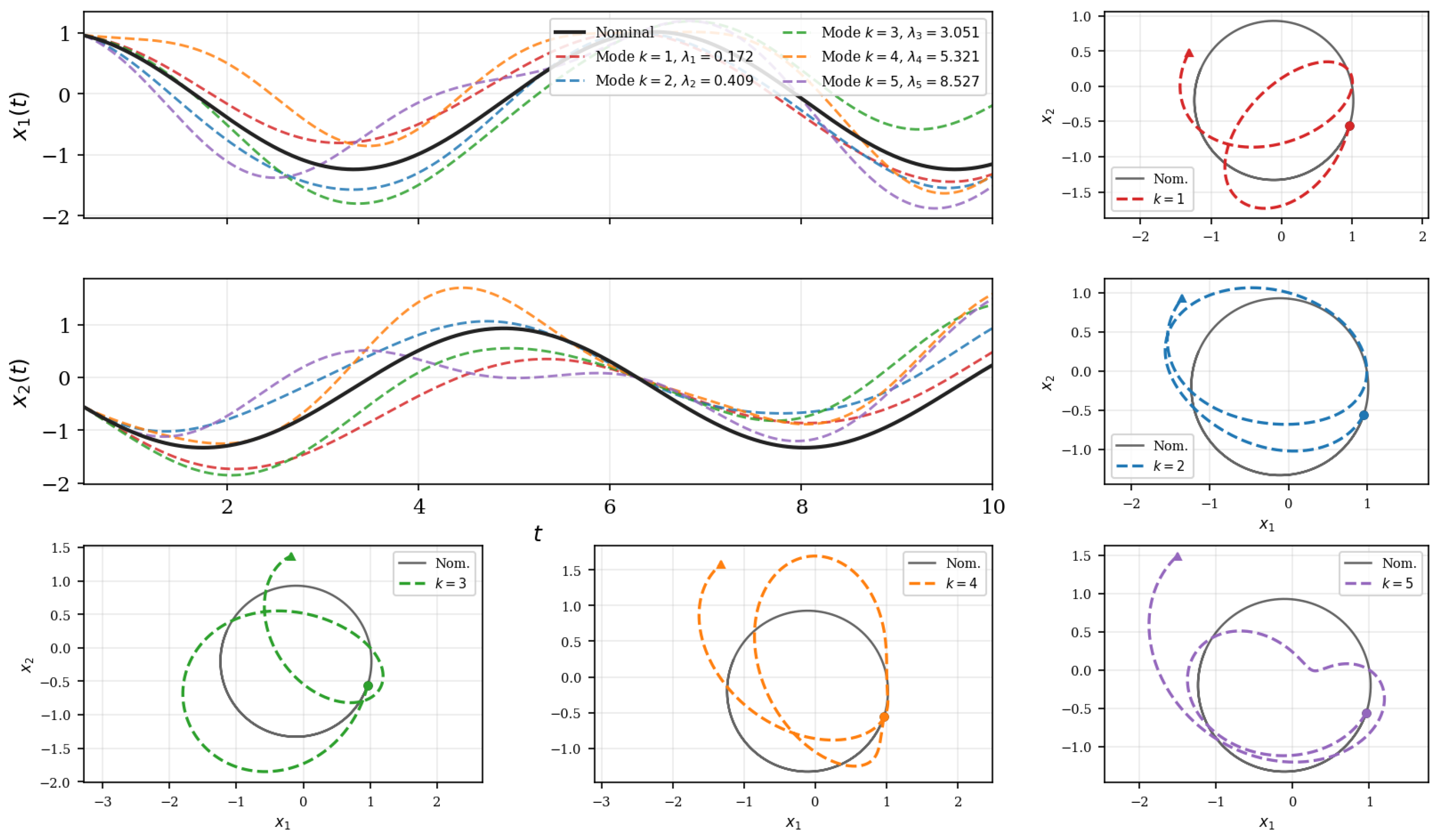
Figure 2 shows the mode-optimal paths directly in the two-dimensional parameter space $({\theta }_1,{\theta }_2)$. All curves originate and terminate near the nominal ${\theta }_0$, forming loops whose shape reflects the basis structure of the eigenfunction ${\eta }^{\left(k\right)}\left(t\right)=({\eta }_1^{\left(k\right)}\left(t\right),{\eta }_2^{\left(k\right)}\left(t\right))$. Mode 1 executes the widest, smoothest excursion — consistent with it having the smallest Rayleigh quotient $\mathcal{R}\left[{\eta }^{\left(1\right)}\right]={\lambda }_1$ and therefore the lowest informational leakage per unit of kinetic work. Higher modes wind more tightly, reflecting the increasing oscillatory frequency ${\omega }_j=(2j-1)\pi /\left[2(b-a)\right]$ of the corresponding basis functions.

Figure 2. Mode-optimal trajectories $({\theta }_1\left(t\right),{\theta }_2\left(t\right))$ in the two-dimensional parameter space for $k=1,\dots ,5$, $K_0=1$. Filled circle: nominal ${\theta }_0$; open circles: $t=a$; triangles: $t=b$.

Figure 2. Mode-optimal trajectories $({\theta }_1\left(t\right),{\theta }_2\left(t\right))$ in the two-dimensional parameter space for $k=1,\dots ,5$, $K_0=1$. Filled circle: nominal ${\theta }_0$; open circles: $t=a$; triangles: $t=b$.

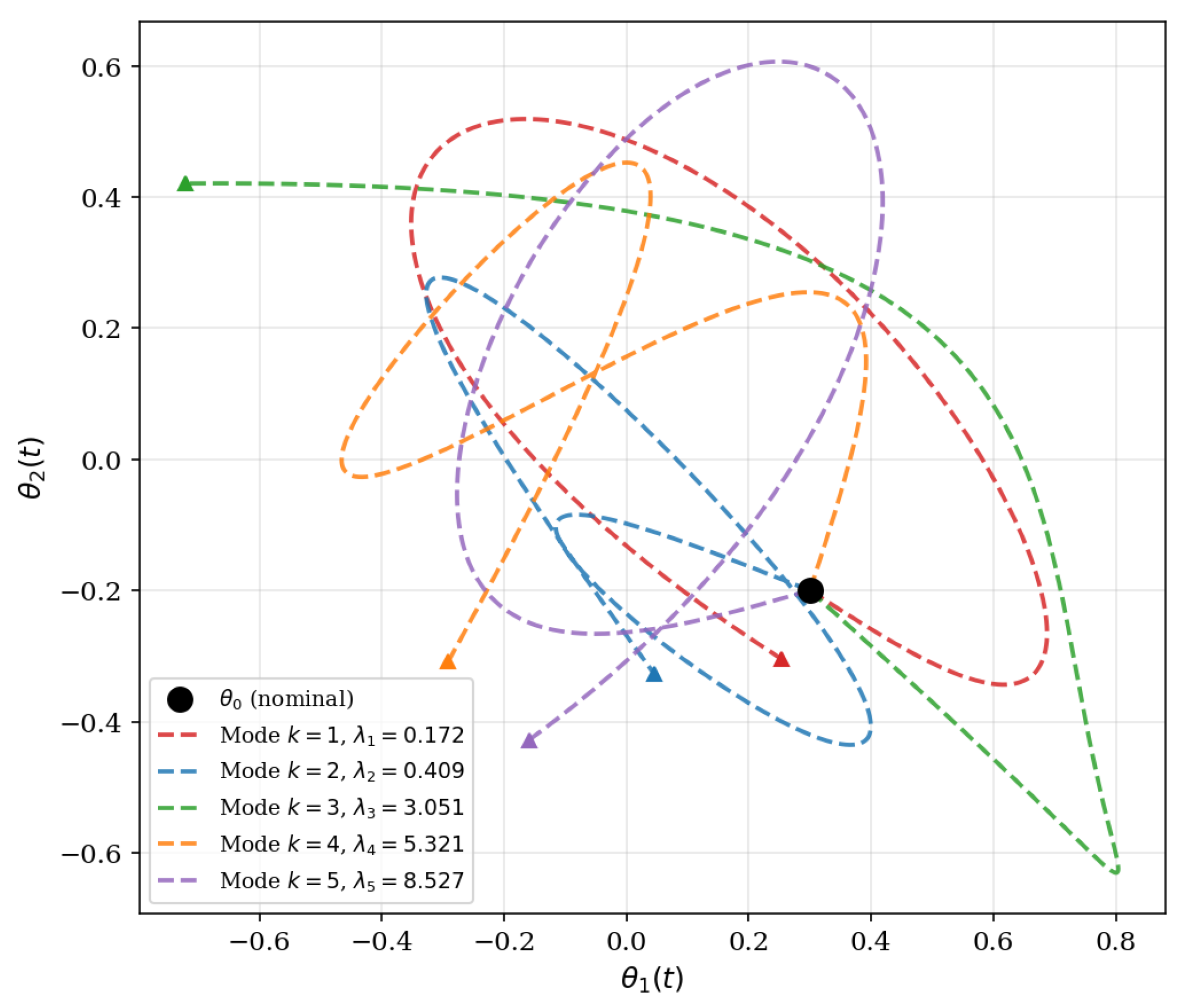
Figure 3 plots the cumulative privacy factor ${\Pi }_{\mathrm{abs}}\left(t\right)=\exp (-D_{KL}\left(t\right))$, where $D_{KL}\left(t\right)$ is evaluated via the closed-form expression (64). All curves start at $\Pi =1$ at $t=a$ (no information yet) and decrease monotonically as the observer accumulates measurements. The ordering

$${\Pi }_{\mathrm{abs}}^{\left(1\right)}\left(t\right)\ge {\Pi }_{\mathrm{abs}}^{\left(2\right)}\left(t\right)\ge \dots \ge {\Pi }_{\mathrm{abs}}^{\left(5\right)}\left(t\right)\forall t\in [a,b]$$

(70)

holds throughout, in agreement with the eigenvalue ordering ${\lambda }_1\le {\lambda }_2\le \dots$ and Corollary 5: among all trajectories with the same kinetic budget $K_0$, the first eigenfunction ${\eta }^{\left(1\right)}$ minimises the KL divergence and therefore maximises the privacy factor at every time instant.

Figure 3. Privacy factor ${\Pi }_{\mathrm{abs}}\left(t\right)=\exp (-D_{KL}\left(t\right))$ along each mode-optimal trajectory ($K_0=1$). Mode $k=1$ (lowest ${\lambda }_1$) decays most slowly, confirming that it is the least detectable path at any fixed kinetic budget.

Figure 3. Privacy factor ${\Pi }_{\mathrm{abs}}\left(t\right)=\exp (-D_{KL}\left(t\right))$ along each mode-optimal trajectory ($K_0=1$). Mode $k=1$ (lowest ${\lambda }_1$) decays most slowly, confirming that it is the least detectable path at any fixed kinetic budget.

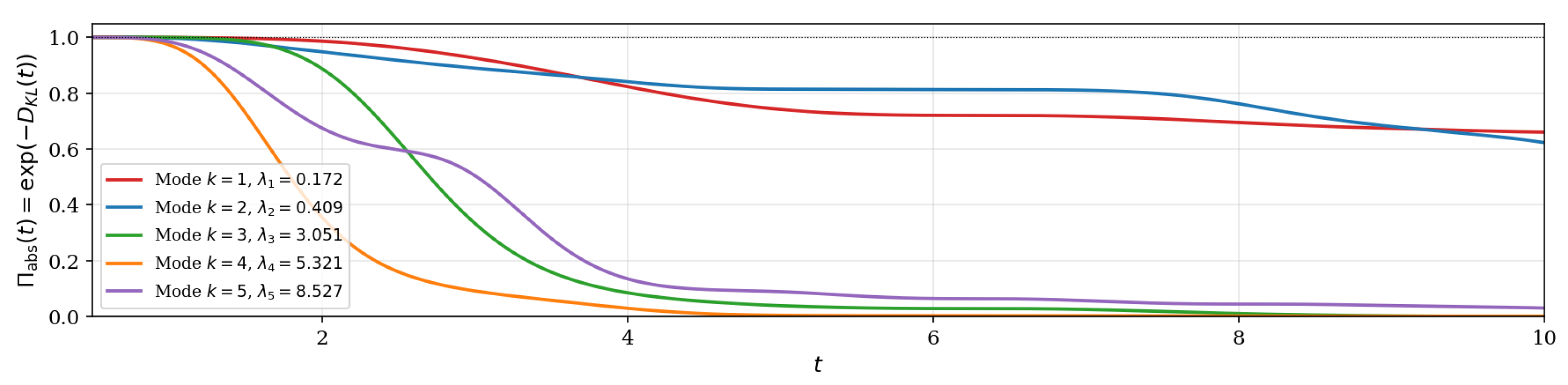
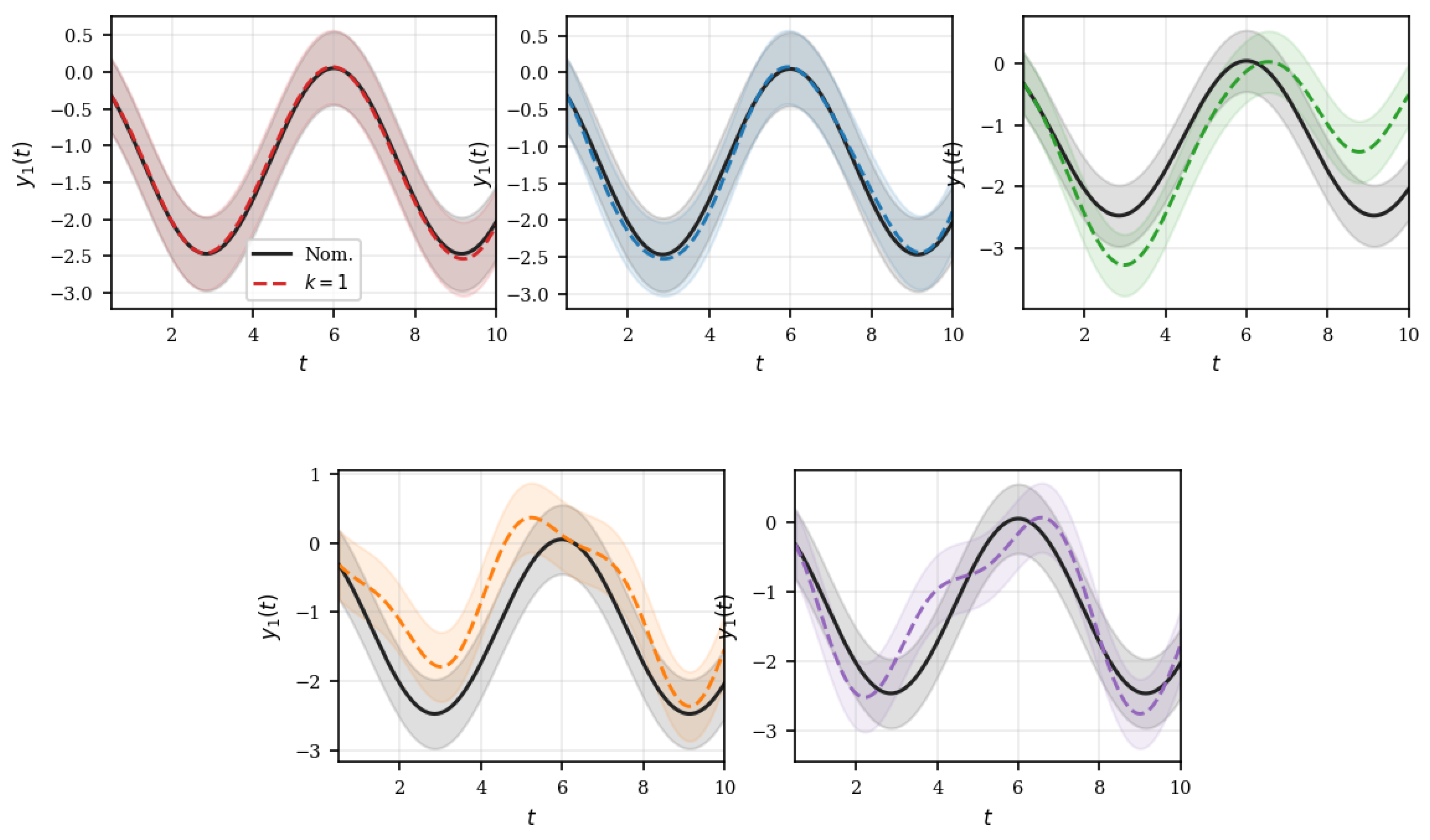
Figure 4 isolates the first observation channel $y_1\left(t\right)$, the quantity directly accessible to the adversary. Each panel compares the nominal mean ${\mu }_1^{\mathrm{nom}}\left(t\right)$ (black) with the mode-optimal mean ${\mu }_1^{\left(k\right)}\left(t\right)$ (colour), both surrounded by the constant $\pm {\sigma }_1$ noise band arising from $\mathrm{Var}\left(y_1\left(t\right)\right)={\sigma }_1^2$. At every instant t, the adversary observes a single draw from $\mathcal{N}({\mu }_1(t,\theta \left(t\right)),{\sigma }_1^2)$ and must decide whether the underlying path is nominal or mode-optimal. The noise band has fixed width, so distinguishability depends on the ratio of the mean displacement $|{\mu }_1^{\left(k\right)}-{\mu }_1^{\mathrm{nom}}|$ to the standard deviation ${\sigma }_1$. Modes with smaller ${\lambda }_k$ keep this ratio small, quantifying the privacy gain identified by Corollary 5.

Figure 4. First observation channel $y_1\left(t\right)$ for modes $k=1,\dots ,5$ vs. nominal. Solid lines: conditional means ${\mu }_1(t,{\theta }^{\left(k\right)}\left(t\right))$. Shaded bands: $\pm {\sigma }_1$ constant noise envelope (${\sigma }_1=0.5$). Panels are arranged in two rows of three and two (centred) respectively.

Figure 4. First observation channel $y_1\left(t\right)$ for modes $k=1,\dots ,5$ vs. nominal. Solid lines: conditional means ${\mu }_1(t,{\theta }^{\left(k\right)}\left(t\right))$. Shaded bands: $\pm {\sigma }_1$ constant noise envelope (${\sigma }_1=0.5$). Panels are arranged in two rows of three and two (centred) respectively.

Theorem 3 guarantees that ${\lambda }_k^{\left(N\right)}\downarrow {\lambda }_k$ as $N\to \infty$, monotonically and from above. We document this convergence numerically by computing the generalized eigenvalues (49) for the system introduced above on a sequence of Galerkin spaces of increasing dimension $N=Jq$, $J=2,4,8,16,32$. Table 1 reports the first five eigenvalues ${\lambda }_1^{\left(N\right)},\dots ,{\lambda }_5^{\left(N\right)}$ together with the relative error ${\mathrm{err}}_k^{\left(N\right)}:=({\lambda }_k^{\left(N\right)}-{\lambda }_k^{★})/{\lambda }_k^{★}$, where ${\lambda }_k^{★}:={\lambda }_k^{\left(N_{\max }\right)}$ is the reference value computed at $N_{\max }=256$.

Two qualitative features of Table 1 are predicted by the theory and are visible in the data: (i) monotone decay of ${\lambda }_k^{\left(N\right)}$ in N at fixed k, in agreement with Theorem 3(i); (ii) approximate algebraic decay ${\lambda }_k^{\left(N\right)}-{\lambda }_k\sim N^{-r}$ with $r\approx 2$ empirically. The exponential decay rate guaranteed by Theorem 3 for $C^{\infty }$ data is therefore not yet reached at $N=256$: the sequence ${\lambda }_1^{\left(N\right)}$ is approaching a limit close to 0, which reflects the near-degeneracy of the spectrum for the undamped oscillator on the relatively long window $[a,b]=[0.5,10]$. This near-degeneracy is consistent with Proposition 4 and Remark 4: for the present system the Poincaré-absorbed coercivity constant $\alpha -\left|\beta \right|/C_P$ is small but positive, so ${\lambda }_1>0$, yet the spectral gap to 0 is itself small. Note that the privacy-factor bound of Corollary 5 remains valid for any value of ${\lambda }_1$ and is therefore not affected by the slow convergence; what the table quantifies is how much resolution is required to obtain a tight numerical estimate of the bound, not its validity.

The bound (63), ${\overline{\Pi }}_{\mathrm{abs}}(P_{\gamma }\parallel Q)\ge \exp (-\frac{1}{2}(b-a){\lambda }_1{K}_0)$, is obtained through one Cauchy–Schwarz and one Jensen step in the proof of Theorem 4.

The bound of Theorem 4 reads $D_{KL}(P_{\gamma }^{\left(T\right)}\parallel Q^{\left(T\right)})\le {\displaystyle \frac{{(b-a)}^2}{2\Delta t}}\tilde{E}\left[\gamma \right]+R(\Delta t)$, where the leading term grows as $1/\Delta t$ and $R(\Delta t)$ is bounded as $\Delta t\to 0$. Similarly, the exact expression (64) for the linear Gaussian case satisfies $D_{KL}\sim I_k{c}^2/\Delta t$ along the k-th eigenmode (Equation (66)). Both the exact divergence and the bound therefore scale as $1/\Delta t$: finer sampling accumulates more information, and the bound tracks this growth proportionally.

Table 2 demonstrates this by reporting, along the first eigenmode ${\gamma }^{\left(1\right)}$ with $K_0=1$ and ${\lambda }_1\approx 0.000274$, the exact KL divergence (64), the leading bound ${\displaystyle \frac{{(b-a)}^2}{2\Delta t}}{\lambda }_1$, and their ratio ${\tau }_1\left(T\right)$, for four values of T (equivalently, four values of $\Delta t=(b-a)/T$).

Three observations follow from Table 2. First, as T increases ($\Delta t$ decreases), both the exact divergence and the bound grow proportionally to $1/\Delta t$, confirming the asymptotic scaling predicted by (66) and Theorem 4. Second, the ratio ${\tau }_1\left(T\right)$ converges rapidly (already within $4\%$ of its limit at $T=50$), so the $O(\Delta t)$ correction term $R(\Delta t)$ is negligible even at coarse sampling. Third, the bound overestimates the exact divergence by a factor $1/{\tau }_1^{\infty }\approx 5000\times$ at all resolutions; this factor is a property of the system (the shape of ${\eta }^{\left(1\right)}$ relative to $\delta \dot{\mu }$), not of the discretisation. Consequently, the qualitative ordering ${\overline{\Pi }}_{\mathrm{abs}}^{\left(1\right)}\ge {\overline{\Pi }}_{\mathrm{abs}}^{\left(2\right)}\ge \dots$ and the privacy bound of Corollary 5 are robust with respect to the choice of $\Delta t$.

References

- Kullback, S. Information Theory and Statistics; John Wiley & Sons: New York, NY, USA, 1959.
- Cover, T.M.; Thomas, J.A. Elements of Information Theory, 2nd ed.; Wiley-Interscience: Hoboken, NJ, USA, 2006.
- Amari, S.; Nagaoka, H. Methods of Information Geometry; Translations of Mathematical Monographs, Vol. 191; American Mathematical Society: Providence, RI, USA, 2000.
- Karatzas, I.; Shreve, S.E. Brownian Motion and Stochastic Calculus, 2nd ed.; Graduate Texts in Mathematics, Vol. 113; Springer: New York, NY, USA, 1991.
- ksendal, B. Stochastic Differential Equations: An Introduction with Applications, 6th ed.; Universitext; Springer: Berlin, Germany, 2003. [CrossRef]
- Barron, A.R. The strong ergodic theorem for densities: Generalized Shannon–McMillan–Breiman theorem. Ann. Probab. 1985, 13, 1292–1303. [CrossRef]
- Pinsker, M.S. Information and Information Stability of Random Variables and Processes; Holden-Day: San Francisco, CA, USA, 1964.
- Gray, R.M. Entropy and Information Theory, 2nd ed.; Springer: New York, NY, USA, 2011.
- Babuška, I.; Osborn, J. Eigenvalue problems. In Handbook of Numerical Analysis; Ciarlet, P.G., Lions, J.L., Eds.; North-Holland: Amsterdam, The Netherlands, 1991; Volume II, pp. 641–787.
- Boffi, D. Finite element approximation of eigenvalue problems. Acta Numer. 2010, 19, 1–120. [CrossRef]
- Chernoff, H. A measure of asymptotic efficiency for tests of a hypothesis based on the sum of observations. Ann. Math. Stat. 1952, 23, 493–507. [CrossRef]
- Csiszár, I.; Shields, P.C. Information theory and statistics: A tutorial. Found. Trends Commun. Inf. Theory 2004, 1, 417–528. [CrossRef]
- van der Vaart, A.W. Asymptotic Statistics; Cambridge Series in Statistical and Probabilistic Mathematics; Cambridge University Press: Cambridge, UK, 1998.
- Tsybakov, A.B. Introduction to Nonparametric Estimation; Springer Series in Statistics; Springer: New York, NY, USA, 2009.
- Le Cam, L. Asymptotic Methods in Statistical Decision Theory; Springer Series in Statistics; Springer: New York, NY, USA, 1986.
- Duchi, J.C. Lecture Notes for Statistics 311 / Electrical Engineering 377: Information Theory and Statistics; Stanford University: Stanford, CA, USA, 2019.
- Brezis, H. Functional Analysis, Sobolev Spaces and Partial Differential Equations; Universitext; Springer: New York, NY, USA, 2011.
- Rudin, W. Principles of Mathematical Analysis, 3rd ed.; McGraw-Hill: New York, NY, USA, 1976.
- Dwork, C.; Roth, A. The algorithmic foundations of differential privacy. Found. Trends Theor. Comput. Sci. 2014, 9, 211–407.
- Le Ny, J.; Pappas, G.J. Differentially private filtering. IEEE Trans. Autom. Control 2014, 59, 341–354.
- Cortés, J.; Dullerud, G.E.; Han, S.; Le Ny, J.; Mitra, S.; Pappas, G.J. Differential privacy in control and network systems. In Proceedings of the 55th IEEE Conference on Decision and Control (CDC), Las Vegas, NV, USA, 12–14 December 2016; pp. 4252–4272.
- Sankar, L.; Rajagopalan, S.R.; Poor, H.V. Utility–privacy tradeoffs in databases: An information-theoretic approach. IEEE Trans. Inf. Forensics Secur. 2013, 8, 838–852. [CrossRef]
- Issa, I.; Wagner, A.B.; Kamath, S. An operational approach to information leakage. IEEE Trans. Inf. Theory 2020, 66, 1625–1657. [CrossRef]
- Mohajerin Esfahani, P.; Sutter, T.; Kuhn, D.; Lygeros, J. From infinite to finite programs: Explicit error bounds with applications to approximate dynamic programming. SIAM J. Optim. 2018, 28, 1968–1998. [CrossRef]
- Nekouei, E.; Tanaka, T.; Skoglund, M.; Johansson, K.H. Information-theoretic approaches to privacy in estimation and control. Annu. Rev. Control 2019, 47, 412–422. [CrossRef]
- Farokhi, F.; Sandberg, H. Fisher information as a measure of privacy: Preserving privacy of households with smart meters using batteries. IEEE Trans. Smart Grid 2017, 9, 4726–4734. [CrossRef]