

Submitted:
16 August 2026
Posted:
18 August 2026
You are already at the latest version
Abstract
Calculation of nonbonded interactions has been a bottleneck for molecular simulations (for molecular dynamics (MD) and Monte Carlo (MC) simulations) that are limiting the system size and the time scale in MD up to nanoseconds. To reduce the computation time/load in calculating nonbonded interactions, an efficient sampling techniques were introduced in this study, for calculating total potential acting on individual atoms. Conventional way of calculating nonbonded interaction for a particular atom is by calculating pairwise van Der Waal and Coulomb interactions for all neighboring atoms with in cutoff radius and adding tail correction beyond the cutoff. Here, we introduce Theory of Local Sampling (TLS), where nonbonded interactions will be calculated by using selective local region around the atom (instead of considering all region within cutoff). Basic principle in TLS is that, any effect/change in global region will reflect in selective local region and can be integrated into molecular simulations. This local sampling technique, instead of global sampling, helps in reducing total computation time/load in calculating nonbonded interactions for the system at each step in MD and in MC simulations. Applying TLS in MD simulation for Argon atoms gives reduction in computation time up to 60%. For MC simulation, up to 37% of reduction in computation time was acheived. Energies and radial distribution function (RDF) comparison for Argon liquid system gives good agreement with conventional MC and MD simulations. Another approach presented in reducing computation time in MD simulations is using "Curve Fitting" techniques in predicting force/acceleration acting on individual atoms using previous time steps, giving 24% reduction in computation time. Combining "TLS & Curve Fitting" techniques further reduces computation time up to 67% in MD simulations.
Keywords:
molecular dynamics
; monte carlo
; theory of local sampling
; reduced computation time
; acceleration prediction
; curve fitting techniques
1. Introduction
Molecular simulations provide valuable insights at atomic/molecular level of phenomenon like multiphase systems, dissolutions, mixing systems [1]. These insights help in modeling systems with understanding from atomic/molecular level. Both MD and MC simulations collect atomic configurations that can lead to evaluate thermodynamic properties where MD simulations collect configurations over time steps and in MC simulations collect configurations by making random moves which can accept/reject the move based on acceptance rule.
Monte Carlo (MC) [2] and molecular dynamics (MD) [3] simulations were first developed in 1950s. Liquid Argon MD simulation was first developed by Rahman [4] in 1964, using Lennard-Jones potentials for Argon atoms. Many studies [5,6,7] leads to the development of MD simulation studies followed with algorithmic improvements. NVT and NPT ensembles in MD simulations were developed later by Andersen [8], Parrinello and Rahman [9,10] followed by development of Nosé-Hoover thermostat [11,12,13]. In MC simulations, collecting configurations by making random moves with accepted/rejected moves with acceptance rule technique was first introduced in the early 1950s at Los Alamos [14]. The Metropolis algorithm introduced random moves with accepted/rejected with probability so that low-energy states are sampled with probability [14]. Hastings [15] in 1970 later developed the algorithm called as Metropolis-Hastings method that was widely used today. Later developments in MC algorithms like Gibbs ensemble Monte Carlo method [16] and configurational-bias Monte Carlo method [17] together with modern high performance computing power have made MC simulations used for studying vapor/liquid systems and biological systems [18].
Calculation of nonbonded interactions has been a bottleneck for conventional molecular simulations (for MD and for MC simulations) that are limiting the system size and collecting the volume of atomic configurations. For all atom model, MD simulations last up to several nanoseconds (ns) with maximum number of atoms in the order of [1]. To perform molecular simulations at higher time scales from nanoseconds to microseconds, development of new theories in molecular simulations are required. With increasing demand for energy supplies, new developments in MC and in MD simulations are needed, that reduce computation cost for each MD or MC step that further reduce cost for maintaining high performance computing facilities.
In this study, Theory of Local Sampling (TLS) was introduced and applied to molecular simulations to reduce computation time in MC and in MD simulations. Theory of Local Sampling (TLS) was first introduced in 2019, in my previous studies (as future work) [19], with noticed reduction in computation time in MC and in MD simulations. TLS can also be applied to other fields where properties are calculated using global regions, like Computational Fluid Dynamics, Stock Market, ab initio molecular simulations, and quantum calculations. Another technique introduced in this study was using curve fitting methods to predict force/acceleration acting on atoms in MD simulations using previous time steps instead of calculating force/acceleration from conventional methods, which reduces computational load. Higher-order function approximations and curve fitting techniques [20] can be implemented to reduce significant computation time.
In the remainder of this paper, working principle of Theory of Local Sampling (TLS) will be introduced in the next section followed by "Simulation Details" of simulations performed in this study. Detailed analysis were presented in "Results and Discussion" section regarding implementation of TLS in MC and in MD simulations, followed by Conclusion section.
2. Introduction to Theory of Local Sampling (TLS)
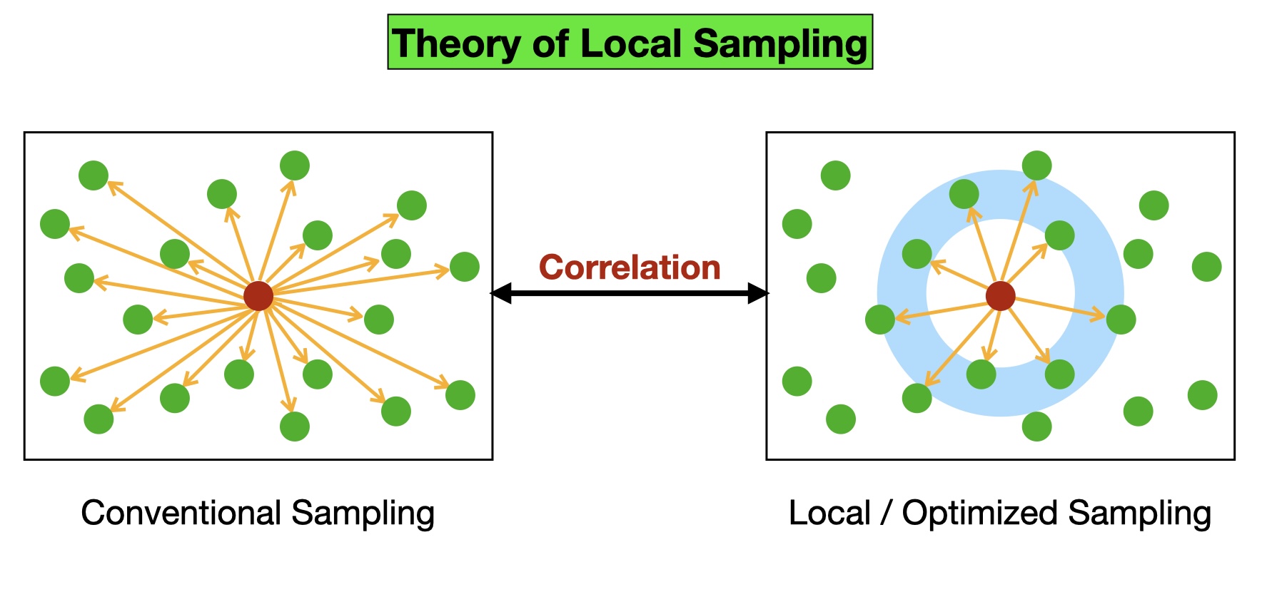
Theory of Local Sampling (TLS) is an efficient sampling technique in calculating nonbonded interactions that reduces total computation time in MC and in MD simulations. Conventional way of calculating nonbonded interaction for a particular atom includes calculating pairwise van Der Waals and Coulomb interactions for all neighboring atoms with in cutoff radius and adding tail correction beyond cutoff radius. In Theory of Local Sampling where, nonbonded interactions will be calculated by using selective local region around the atom, that carries and contains information of global region. Instead of considering global/all region around an atom, considering local regions was more optimized way for calculating nonbonded interactions, in MC and in MD simulations, as shown in Figure 1. Local region in TLS can be a sphere around an atom, with inner radius (x1) and outer radius (x2) (called as "Bin Width" in this study). In MC simulation, considering local region, that carries information of global region that will reflect in calculating "acceptance rule". Similarly, in MD simulations, calculating force/acceleration acting on an atom based on local region gives good agreement with conventional MD simulations, as reported in this study. TLS technique helps in reducing total computation time in calculating nonbonded interactions for the systems at each simulation step. The number of arrows in Figure 1 which represents pairwise potential calculations required in MC and MD simulations, decreased significantly between conventional/global sampling and local/optimized sampling.
Main principle involved in TLS is any small change in global region of a system will reflect in the considered local region and can model the whole system by correlating between global and local region, as shown in Figure 1. TLS is considered to be efficient sampling technique where properties can be modeled by using local sample than sampled globally in a conventional way. Other types of local regions can be considered like a cube or cylindrical ring around the atom, or wavy surface of cos/sin function around the atom, depending on the system, that can give more optimized local sampling in TLS.
Theory of Local Sampling in molecular simulations can be implemented as follows:
- Bin width around an atom (with friction in RDF plots, at the end of bin width).
- Bin width around an atom with varying bin size randomly at each time step (without friction in RDF plots).
- Randomly chosen samples around atom with or without bin width around an atom.
- Considering multiple local regions instead on one local region.
Correlation between local sampling and global sampling can be a captured by modeling the amount of error estimated between global and local region property values. Neural networks and artificial intelligence (AI) are some of the tools that can be integrated in TLS in molecular simulation that will take simulation to higher time scale from nanoseconds to microseconds in MD simulations. With depleting fossil fuel reserves and increase in global warming effects in the past few decades, efficient methods in saving energy is very much needed for power requirements of high performance computing facilities to run molecular simulations for bigger systems.
In this study, results of Theory of Local Sampling (TLS) were reported for MC simulations, MD Simulations, "Curve Fitting in MD simulations" and "TLS & Curve Fitting MD simulations" with significant reduction in computation time. By applying TLS in MC simulations, reduction in computation time was achieved up to 37% and in MD simulations, up to 67% reduction was achieved, as shown in the following sections.
Another approach in molecular simulations to reduce computation time is using "Local Function" instead of conventional potential functions for calculating potential acting on an atom. Idea behind this approach is local function for potential calculation requires less computational load, where conventional potential functions demands higher computational load. Later exact force/potential acting on atom can be deduced by extrapolating/correlating the local function with conventional potential functions. TLS sampling techniques can be applied to systems where properties of single atom/point were estimated by global sampling around the atom/point considered. Systems like ab initio molecular simulations, quantum simulations, Computational Fluid Dynamics (CFD), and dynamics of stock market, where global properties can be estimated by considered local population/local sampling and scaling/correlating back to global values.
3. Simulation Details
Argon system of 500 atoms was used to study the implentation of Theory of Local Sampling (TLS) in Monte Carlo and in Molecular Dynamics simulations. MC and MD simulation codes for Argon atoms were developed using fortran language. 500 Argon atoms were considered in a simulation box with density of 1400 kg/m3. Lennard Jones parameters for argon atoms for as 3.4 Åand as 1.65*10−21 Joules were considered in this study [21]. For nonbonded interactions, cutoff radius of 14 Åwas used and tail correction was applied to atoms beyond the cutoff. Periodic boundary conditions were applied in all directions in a simulation box using Minimum Image Convention algorithm. For MD simulations, Velocity Verlet integrator [22] was used with initial velocities given to argon atoms using Gaussian distribution at 86 K. Velocity rescaling algorithm [23] was implemented at temperature of 86 K. Dimensionless time step of 0.01 was used in MD simulations. Bin width (x1* - x2*) for TLS is defined as a local region around an atom with inner radius of x1* and outer radius of x2*, making it a sphere region around an atom, as shown in Figure 1. Radial distribution function (RDF) plots and all other variables reported in this study are dimensionless variables (x* = r/) with dimensionless bin widths (x1* - x2*) that are considered for local regions in TLS. For MC simulations, dimensionless distance (dx* = dr/) of 0.1 was used to move the atoms randomly at each MC cycle (trail move). Both MC and MD simulations were performed for 100,000 steps to calculate the required computation time. Computation time for both MC and for MD simulations were reported in this study using single processor. Average properties like potential energy, kinetic energy, and temperature of the argon system were calculated for the last 2000 steps for MC and MD simulations with dimensionless values reported in this study. For "Curve Fitting Algorithm in MD simulation", computational load for calculating potential energies at fourth step is excluded.
4. Results and Discussions
4.1. Theory of Local Sampling in Monte Carlo Simulations
TLS was applied to MC simulations (known as "TLS MC") for Argon atoms, for calculating potential acting on an atom by considering local region instead of global region (all region around the atom) with various bin width, as shown in Table 1. Bin width (x1* - x2*) were considered with minimum bin width of (0.5 - 1.5) to maximum bin width of (0.5 - 2.0). For calculating "acceptance rule", to accept or reject a random move of an atom, potential energies of new trail move (E2) and potential energy before trail move (E1) were calculated in the local region. The differences of conventional potential energies values, in acceptance rule, will be reflected (in lower magnitude) in the considered local region, which is the basic principle of Theory of Local Sampling. Maximum of 37% of reduction in computation time was achieved for bin width of (0.5 - 1.5) for "TLS MC" simulation when compared with conventional MC simulation, as shown in Table 1. Conventional MC simulation takes 579.6 seconds to complete 100,000 MC cycles, where as "TLS MC" simulation takes a minimum of 363.8 seconds for the same Argon system, with reduction in computation time 37%. Percentage of reduction in computation time decreases with increase in bin width of local region from (0.5 - 1.5) to (0.5 - 2.0) for "TLS MC" simulation.
Potential energies calculated for conventional MC, "TLS MC" simulation with bin width of (0.5 - 1.5) and (0.5 - 2.0) was shown in Figure 2. It was observed that atomic configurations of "TLS MC" were different from conventional MC simulation as potential energies having unique atomic configurations over MC cycles. Observation of Figure 2 shows that "TLS MC" simulation with bin width of (0.5 - 2.0) and conventional MC simulation have merged potential values after 1300 MC cycles. Average PE* for bin (0.5 - 1.5) is lower than conventional MC simulation as shown in Figure 2 and Table 1.
Radial distribution function plots were considered for comparing atomic configuration distribution at equilibrium stage for conventional MC and "TLS MC" simulation, as shown in Figure 3. For "TLS MC" simulation, RDF plots shows a friction or discontinuity in atom distribution at the end of bin width, as shown in Figure 3 for bin widths of (0.5 - 1.5) and (0.5 - 2.0). "TLS MC" simulation follows maximum and minimum peaks of first, second, and third solvation shells, when compares to conventional MC simulations. One of the reason for having friction in atoms distribution around local region bin width is "Acceptance rule" is considered only for the local region and atoms in remaining regions have to adjust itself, creating a shock wave or friction at the end of outer radius of bin width (x2*). To reduce the shock or friction in atom distribution at the end of bin width, outer radius bin width size (x2*) was varied randomly at the magnitude of 0.4 units at each trail move of atoms in each MC cycle. Variation of outer radius bin width size at each trail move reduces shock in atom distribution and atoms will adjust itself at all regions instead of only at local region bin width. Table 2 shows "TLS MC" simulation with varying bin width randomly from (0.5 to 1.3-1.7) to (0.5 to 2.0-2.4), with maximum reduction in computation time of 36%. Figure 4 show RDF plots comparison for conventional MC simulation to "TLS MC" simulation with varying bin width size, with no friction in RDF curves unlike in Figure 3. It is clear that, varying bin width at each trail move of an atom, reduces shock/friction in equilibrium atomic configurations as shown in Figure 3 and Figure 4.
4.2. Theory of Local Sampling in Molecular Dynamics Simulations
Theory of local sampling (TLS) was applied to MD simulation (TLS MD) of Argon atoms for calculating force acting on an atom that further used in calculating acceleration of an atom that was used in Velocity Verlet Algorithm at each time step. For "TLS MD" simulations, local regions were selected with inner and outer radius (x1* - x2*) (bin width) for each atom, for calculating force acting using Lennard-Jones potential. Conventional MD simulations for 500 Argon atoms were performed and compared with "TLS MD" as shown in Table 3. Maximum of 60% reduction in computation time was achieved for "TLS MD" with bin width of (0.75 - 1.25) when compared with conventional MD simulation. Conventional MD simulation takes 324.1 seconds to complete for 100,000 steps using single processor, while "TLS MD" simulation takes minimum of 130.6 seconds (60% reduction in total computation time) for the same system. For bin width (0.75 - 1.25), average potential energy slightly differs between conventional MD and "TLS MD" with values -2996.5 and -2936.3 (dimensionless potential energies, PE*), respectively. As bin width increases from (0.75 - 1.25) to (0.75 - 2.2), average potential energy decreases and came closer to conventional MD simulation energies, as shown in Table 3. Temperature of "TLS MD" and conventional MD maintain same consistency irrespective of bin width chosen for "TLS MD", as velocity rescale thermostat was used in both cases. Reduction in computation time decreases with increase in bin width size, from (0.75 - 1.25) to (0.75 - 2.2), with minimum values achieved for 50% reduction. Minimum potential energy of the Argon system was achieved in "TLS MD" of -3009.8 when compared to conventional MD simulation (-2996.5), indicating more optimized phase space configurations were achieved in "TLS MD" than in conventional MD simulation.
Comparison of potential energy (PE) for "TLS MD" with conventional MD was shown in Figure 5, with bin width of (0.75 - 1.25) and (0.75 - 1.8). "TLS MD" phase space has its unique movement over MD time steps when compared to conventional MD simulation. It was observed that bin width of (0.75 - 1.8) have closer potential energies with conventional MD simulation. Average PE for bin width (0.75 - 1.25) is higher than conventional MD simulation, as shown in Figure 5 and Table 3.
Radial distribution function (RDF) for conventional MD and "TLS MD" were considered to study the atomic distributions after reaching equilibrium. Figure 6 shows RDF plots for conventional MD and "TLS MD" with bin width of (0.75 - 1.25) and (0.75 - 1.8). It was observed that "TLS MD" shows good agreement with conventional MD in first, second, and third solvation shells. For "TLS MD" with bin width of (0.75 - 1.25) have higher peak in first solvation shell which reflects in average potential energy and in PE plot, in Table 3 and Figure 5, respectively. Same happens at the minimum of first solvation shell for "TLS MD" with bin width of (0.75 - 1.25) when compared with conventional MD simulation, as shown in Figure 6. Minimum deviations were found for second, third, and fourth solvation shells between "TLS MD" and conventional MD simulations. Bin width less than (0.75 - 1.25) gives RDF that deviate from RDF of conventional MD simulations, giving different atomic configurations and analysis of such configurations is beyond the scope of this study.
By comparing average energies, average temperature (Table 3), PE plot (Figure 5), and RDF plot (Figure 6), "TLS MD" shows good agreement with conventional MD simulations with reduction in computation time from 50% - 60%. Correlation and extrapolation of force/potential values of local region to global region was not considered in this study.
4.3. Curve Fitting Algorithm for Acceleration Prediction in MD Simulations
Another approach in reducing computation time in MD simulations is predicting/extrapolating properties of future time steps, from previous time steps using function approximations like curve fitting techniques [20], as shown in Figure 7. It was observed that force/acceleration time profiles on a particular atom in MD simulations shows smooth curves with joining splines with quadratic/cubic in nature as shown in Figure 8. Figure 8 shows acceleration time profile in x-axis (ax) for an individual Argon atom in conventional MD simulation for Argon system. It shows that force/acceleration at intermediate steps can be predicted using previous time steps using quadratic/cubic equations. This technique of apply curve fitting techniques show reduction in overall computation time, as intermediate steps are predicted with free of cost in terms of computational load. In this study, acceleration for each Argon atom was predicted at every 4th time step from the previous 3 time steps using quadratic function approximation. For every 4th MD time steps, one MD step is predicting instead of calculating force/acceleration in conventional way which reduces computational load in MD simulation. It was expected to reduce computation time of 25%, since for every 4 time steps, one time step is free of cost. Higher order function approximation [20] for force/acceleration time profiles can be considered to predict two or more time steps ahead using previous time steps, that reduces computation time more than 25% and this approach is beyond the scope of this study.
In this study, acceleration was calculated at every 4th time step by assuming quadratic equation (Equation 1) for acceleration over time. To find the constant of a, b, and c, previous three time steps are considered as -1, 0, 1, time values (Equations 2, 3, and 4), for simplicity. Fourth time step will be calculated as per Equation 5. Constants of a, b, and c were calculated from Equations 6, 7, and 8, using previous acceleration values (ac1, ac2, and ac3). Equation 9 shows acceleration value at every 4th time step (ac4) in terms of acceleration values from previous time steps.
from equations (2), (3), and (4), constants a, b, c were obtained as follows:
Substituting the constants (a, b, and c) in Equation (5) gives acceleration for the present time step (ac4,now) as follows:
Table 4 shows reduction in computation time in apply curve fitting algorithm in MD simulation (called as "Curve Fitting MD") with conventional MD simulation. As predicted, 24% reduction in computation time was achieved with potential energies, kinetic energies and temperature average values shows similar to conventional MD simulations (Table 4).
Figure 9 compares potential energy (PE*) profile for "Curve Fitting MD" and conventional MD for the first 2000 time steps of Argon atoms. During initial time steps, "Curve Fitting MD" follows same as conventional MD profile and later departs by have its own phase space configurations over time. Both MD simulations have average potential values as same with slight variations having their own phase space configurations over time.
RDF plots comparison shows similar atomic distribution for first, second, and third solvation shells for "Curve fitting MD" and conventional MD simulations, as shown in Figure 10.
4.4. Combining TLS & Curve Fitting Algorithm in MD Simulations
Further reduction in computation time in MD simulations can be achieved by combining "TLS MD" and "Curve Fitting MD", where force/potential can be calculated for the first 3 time steps using "TLS MD" and the 4th time step will be predicted using "Curve Fitting MD" technique. Another 10% of overall reduction in computation time will be expected, as 25% reduction in computation time of "TLS MD" will be achieved due to "Curve Fitting MD". Every 4th time step of acceleration value is predicted using previous 3 time steps whose acceleration was calculated using local sampling. Table 5 shows reduction in computation time for "TLS & Curve Fitting MD" when compared with conventional MD simulations along with calculated potential energy, kinetic energy, and temperature average values. Maximum percentage of reduction in achieved by 67% for bin width of (0.75 - 1.25) with minimum value of 61% for bin width of (0.75 - 2.2). Potential energies and kinetic energies shows good agreement with conventional MD simulations as shown in Table 5.
RDF plots comparison for "TLS & Curve Fitting MD" and conventional MD simulation were analyzed for bin widths of (0.75 - 1.25) and (0.75 - 1.8), as shown in Figure 11. RDF plot shows similar behavior as "TLS MD" (Figure 6) and inclusion of "Curve Fitting MD" in "TLS MD" has lesser impact in distribution of atomic configurations after reaching equilibrium.
5. Conclusion
Theory of local sampling (TLS) in molecular simulations was introduced in this study with reported reduction in computation time in MC and in MD simulations. Reduction in computation time up to 60% was achieved in Theory of Local Sampling Molecular Dynamics (TLS MD) and in "TLS MC" simulations up to 37% reduction was achieved. "Curve fitting" techniques was implemented in MD simulations ("Curve Fitting MD") for predicting force/acceleration acting on atom at every 4th step using previous 3 time steps, with achieved reduction in computation time of 24%. Further, combining "TLS MD" and "Curve Fitting MD" reduces more computational time with maximum reduction of 67% was achieved when compared to conventional MD simulation. TLS can be applied to other systems with principle of calculating local sample and scaling back to global sampling values for systems like ab initio molecular simulations, quantum calculations, Computational Fluid Dynamics (CFD), and dynamics of stock/equity market. "TLS MD" using random local sampling, modeling of error estimation with conventional sampling for MD simulations will be another approach to reduce computational load in MD simulations. Neural networks and artificial intelligence (AI) are some of the tools that can be integrated in TLS in molecular simulation that will reduce computation time to many folds.
Acknowledgments
I thank Mississippi State University (MSU) as previous work and previous simulations on Theory of Local Sampling (TLS) were carried out in MSU computers and High performance computing facility as part of my Ph.D. Thesis work. I thank Dr. Neeraj Rai for his valuable discussions on "Nonbonded Interactions" on molecular simulations.
References
- Allen, M. P.; Tildesley, D. J. Computer simulation of liquids; Oxford university press, 2017. [Google Scholar]
- Metropolis, N.; Rosenbluth, A. W.; Rosenbluth, M. N.; Teller, A. H.; Teller, E. Equation of state calculations by fast computing machines. J. Chem. Phys. 1953, 21, 1087–1092. [Google Scholar] [CrossRef]
- Alder, B. J.; Wainwright, T. E.; et al. Phase transition for a hard sphere system. J. Chem. Phys. 1957, 27, 1208. [Google Scholar] [CrossRef]
- Rahman, A. Correlations in the motion of atoms in liquid argon. Phys. Rev. 1964, 136, A405. [Google Scholar] [CrossRef]
- Verlet, L. Computer" experiments" on classical fluids. I. Thermodynamical properties of Lennard-Jones molecules. Phys. Rev. 1967, 159, 98. [Google Scholar] [CrossRef]
- Rahman, A.; Stillinger, F. H. Molecular dynamics study of liquid water. J. Chem. Phys. 1971, 55, 3336–3359. [Google Scholar] [CrossRef]
- McCammon, J. A.; Gelin, B. R.; Karplus, M. Dynamics of folded proteins. nature 1977, 267, 585–590. [Google Scholar] [CrossRef] [PubMed]
- Andersen, H. C. Molecular dynamics simulations at constant pressure and/or temperature. J. Chem. Phys. 1980, 72, 2384–2393. [Google Scholar] [CrossRef]
- Parrinello, M.; Rahman, A. Crystal structure and pair potentials: A molecular-dynamics study. Phys. Rev. Lett. 1980, 45, 1196. [Google Scholar] [CrossRef]
- Parrinello, M.; Rahman, A. Polymorphic transitions in single crystals: A new molecular dynamics method. J. Appl. Phys. 1981, 52, 7182–7190. [Google Scholar] [CrossRef]
- Neusy, E.; Nosé, S.; Klein, M. L. Molecular dynamics calculations for solid bicyclo (2.2. 2) octane. Mol. Phys. 1984, 52, 269–279. [Google Scholar] [CrossRef]
- Nosé, S. A unified formulation of the constant temperature molecular dynamics methods. J. Chem. Phys. 1984, 81, 511–519. [Google Scholar] [CrossRef]
- Hoover, W. G. Canonical dynamics: Equilibrium phase-space distributions. Phys. Rev. A 1985, 31, 1695. [Google Scholar] [CrossRef] [PubMed]
- Metropolis, N.; Rosenbluth, A. W.; Rosenbluth, M. N.; Teller, A. H.; Teller, E. Equation of State Calculations by Fast Computing Machines. J. Chem. Phys. 1953, 21, 1087–1092. [Google Scholar] [CrossRef]
- Hastings, W. K. Monte Carlo Sampling Methods Using Markov Chains and Their Applications. Biometrika 1970, 57, 97–109. [Google Scholar] [CrossRef]
- Panagiotopoulos, A. Z. Direct Determination of Phase Coexistence Properties of Fluids by Monte Carlo Simulation in a New Ensemble. Mol. Phys. 1987, 61, 813–826. [Google Scholar] [CrossRef]
- Siepmann, J. I.; Frenkel, D. Configurational bias Monte Carlo: a new sampling scheme for flexible chains. Mol. Phys. 1992, 75, 59–70. [Google Scholar] [CrossRef]
- Frenkel, D.; Smit, B. Understanding Molecular Simulation: From Algorithms to Applications, 2nd ed.; Academic Press: San Diego, 2002. [Google Scholar]
- Venkatesan, S. S. Algorithmic improvements and applications of molecular dynamics simulations to probe condensed phase systems. Theses and Dissertations, 2019. Available online: https://scholarsjunction.msstate.edu/td/431.
- Gupta, S. K. Numerical methods for engineers; New Age International, 1995. [Google Scholar]
- Rahman, A. Correlations in the Motion of Atoms in Liquid Argon. Phys. Rev. 1964, 136, A405–A411. [Google Scholar] [CrossRef]
- Swope, W. C.; Andersen, H. C.; Berens, P. H.; Wilson, K. R. A computer simulation method for the calculation of equilibrium constants for the formation of physical clusters of molecules: Application to small water clusters. J. Chem. Phys. 1982, 76, 637–649. [Google Scholar] [CrossRef]
- Bussi, G.; Donadio, D.; Parrinello, M. Canonical sampling through velocity rescaling. J. Chem. Phys. 2007, 126, 014101. [Google Scholar] [CrossRef] [PubMed]
Figure 1.
Application of Theory of Local Sampling (TLS) in molecular simulations showing conventional sampling that correlates with local sampling for calculating potential acting on an atom (red circle) from its neighboring atoms.
Figure 1.
Application of Theory of Local Sampling (TLS) in molecular simulations showing conventional sampling that correlates with local sampling for calculating potential acting on an atom (red circle) from its neighboring atoms.
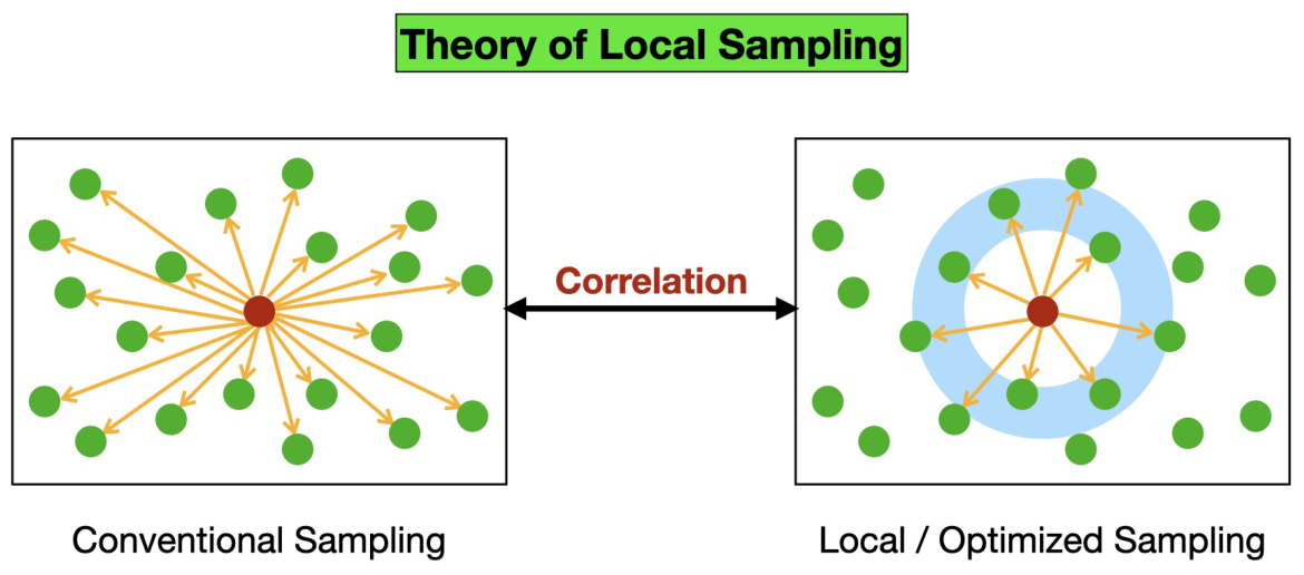
Figure 2.
Comparison of potential energy (PE*) of Argon atoms for conventional MC simulations with Theory of Local Sampling MC simulations (TLS MC) for bin width of (0.5 - 1.5) and (0.5 - 2.0).
Figure 2.
Comparison of potential energy (PE*) of Argon atoms for conventional MC simulations with Theory of Local Sampling MC simulations (TLS MC) for bin width of (0.5 - 1.5) and (0.5 - 2.0).
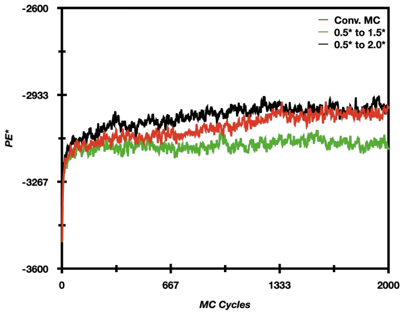
Figure 3.
Comparison of radial distribution function (RDF) of Argon atoms of conventional Monte Carlo with Theory of Local Sampling Monte Carlo (TLS MC) simulations for various bin width.
Figure 3.
Comparison of radial distribution function (RDF) of Argon atoms of conventional Monte Carlo with Theory of Local Sampling Monte Carlo (TLS MC) simulations for various bin width.
Figure 4.
Comparison of radial distribution function (RDF) of Argon atoms of conventional Monte Carlo with Theory of Local Sampling Monte Carlo (TLS MC) simulations for varying bin width size.
Figure 4.
Comparison of radial distribution function (RDF) of Argon atoms of conventional Monte Carlo with Theory of Local Sampling Monte Carlo (TLS MC) simulations for varying bin width size.
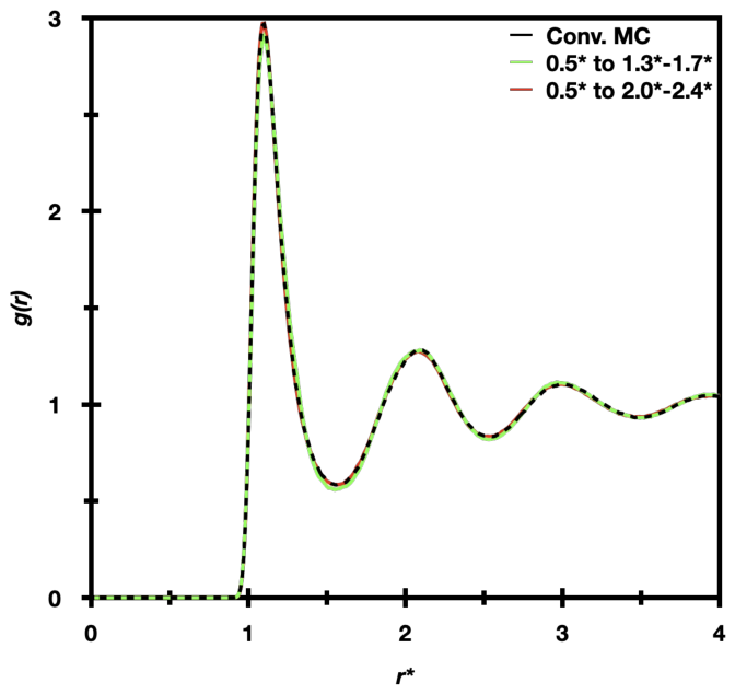
Figure 5.
Comparison of potential energy of Argon atoms for conventional MD simulations (red line) with Theory of Local Sampling MD (TLS MD) simulations for bin width of (0.75 - 1.25) (green line) and (0.75 - 1.8) (black line).
Figure 5.
Comparison of potential energy of Argon atoms for conventional MD simulations (red line) with Theory of Local Sampling MD (TLS MD) simulations for bin width of (0.75 - 1.25) (green line) and (0.75 - 1.8) (black line).
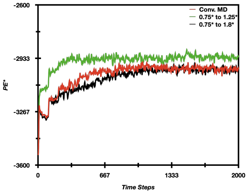
Figure 6.
Comparison of radial distribution function (RDF) of Argon atoms of conventional MD (dashed black line) with Theory of Local Sampling MD (TLS MD) simulations for bin widths of (0.75 - 1.25) (green line) and (0.75 - 1.8) (red line).
Figure 6.
Comparison of radial distribution function (RDF) of Argon atoms of conventional MD (dashed black line) with Theory of Local Sampling MD (TLS MD) simulations for bin widths of (0.75 - 1.25) (green line) and (0.75 - 1.8) (red line).
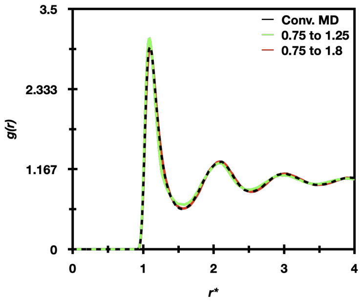
Figure 7.
Applying curve fitting techniques for acceleration curve predicting fourth time step (t2,now) from previous three time steps.
Figure 7.
Applying curve fitting techniques for acceleration curve predicting fourth time step (t2,now) from previous three time steps.
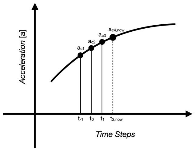
Figure 8.
Acceleration (ax*) curve of first 500 time steps, for a single Argon atom, showing smooth cubic/parabolic splines joined together.
Figure 8.
Acceleration (ax*) curve of first 500 time steps, for a single Argon atom, showing smooth cubic/parabolic splines joined together.
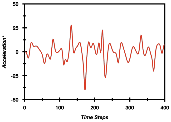
Figure 9.
Comparison of potential energy of Argon atoms for conventional MD simulations with "Curve Fitting MD" simulations.
Figure 9.
Comparison of potential energy of Argon atoms for conventional MD simulations with "Curve Fitting MD" simulations.
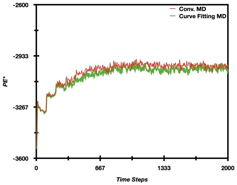
Figure 10.
Comparison of radial distribution function (RDF) of Argon atoms for conventional Molecular Dynamics and "Curve Fitting MD" simulations.
Figure 10.
Comparison of radial distribution function (RDF) of Argon atoms for conventional Molecular Dynamics and "Curve Fitting MD" simulations.
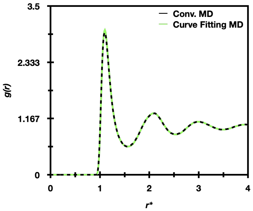
Figure 11.
Comparison of radial distribution function (RDF) of Argon atoms of conventional MD (dashed black line) with "TLS & Curve Fitting Algorithm" MD simulations for bin widths of (0.75 - 1.25) (green line) and (0.75 - 1.8) (red line).
Figure 11.
Comparison of radial distribution function (RDF) of Argon atoms of conventional MD (dashed black line) with "TLS & Curve Fitting Algorithm" MD simulations for bin widths of (0.75 - 1.25) (green line) and (0.75 - 1.8) (red line).
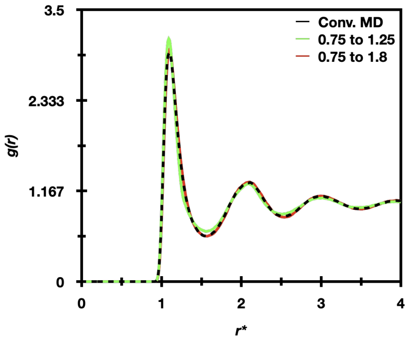

Table 1.
Reduction in Computation Time by applying Theory of Local Sample in Monte Carlo Simulations (TLS MC) for Argon Atoms, showing friction in RDF plot at end of local region.
Table 1.
Reduction in Computation Time by applying Theory of Local Sample in Monte Carlo Simulations (TLS MC) for Argon Atoms, showing friction in RDF plot at end of local region.
| Bin Width Size ( to ) | Average Potential Energy (PE*) | Computation Time (Seconds) | Reduction in Computation Time |
|---|---|---|---|
| Conventional MC | -3002.7 (±16.0) | 579.6 | - |
| 0.5 to 1.5 | -3032.3 (±15.7) | 363.8 | 37% |
| 0.5 to 1.6 | -3010.2 (±16.3) | 376.0 | 35% |
| 0.5 to 1.8 | -2983.6 (±16.8) | 386.4 | 33% |
| 0.5 to 2.0 | -2993.0 (±16.0) | 397.7 | 31% |
| 0.6 to 1.5 | -3035.3 (±15.8) | 367.4 | 37% |
| 0.6 to 1.8 | -2984.2 (±16.2) | 386.1 | 33% |
| 0.7 to 1.5 | -3036.3 (±16.1) | 372.8 | 36% |
| 0.7 to 1.6 | -3009.4 (±18.1) | 376.6 | 35% |
| 0.7 to 1.8 | -2986.3 (±15.5) | 384.0 | 34% |
Table 2.
Reduction in Computation Time by applying Theory of Local Sample in Monte Carlo Simulations for Argon Atoms, for varying bin width and without friction across bin width sampling in RDF plots
Table 2.
Reduction in Computation Time by applying Theory of Local Sample in Monte Carlo Simulations for Argon Atoms, for varying bin width and without friction across bin width sampling in RDF plots
| Varying Bin Width Size ( to Δ) | Average Potential Energy (PE*) | Computation Time (Seconds) | Reduction in Computation Time |
|---|---|---|---|
| Conventional MC | -3002.7 (±16.0) | 579.6 | - |
| 0.5 to 1.3-1.7 | -3010.1 (±15.6) | 373.3 | 36% |
| 0.5 to 1.4-1.8 | -3003.3 (±16.8) | 378.3 | 35% |
| 0.5 to 1.6-2.0 | -2992.4 (±16.7) | 388.2 | 33% |
| 0.5 to 1.8-2.2 | -2988.0 (±16.0) | 397.3 | 32% |
| 0.5 to 2.0-2.4 | -3000.7 (±18.8) | 412.1 | 29% |
Table 3.
Table showing comparison of conventional MD with "TLS MD" with reduction in computation time and comparing properties of average potential energy, kinetic energy, and, temperature
Table 3.
Table showing comparison of conventional MD with "TLS MD" with reduction in computation time and comparing properties of average potential energy, kinetic energy, and, temperature
| Bin Width Size ( to ) | Average Potential Energy (PE*) | Average Kinetic Energy (KE*) | Average Temperature (T*) | Computation Time (Seconds) | Reduction in Computation Time |
|---|---|---|---|---|---|
| Conv. MD | -2996.5 (± 15.8) | 536.5 (± 16.2) | 0.72 (± 0.02) | 324.1 | - |
| 0.75 to 1.25 | -2936.3 (± 13.5) | 538.1 (± 12.7) | 0.72 (± 0.02) | 130.6 | 60% |
| 0.75 to 1.35 | -2971.8 (± 14.9) | 542.3 (± 13.4) | 0.72 (± 0.02) | 132.3 | 59% |
| 0.75 to 1.5 | -3001.9 (± 15.0) | 546.3 (± 15.5) | 0.73 (± 0.02) | 132.8 | 59% |
| 0.75 to 1.65 | -3009.8 (± 13.0) | 542.4 (± 13.8) | 0.72 (± 0.02) | 136.4 | 58% |
| 0.75 to 1.8 | -2996.7 (± 14.8) | 545.0 (± 14.7) | 0.73 (± 0.02) | 141.9 | 56% |
| 0.75 to 2.0 | -2994.5 (± 14.9) | 539.7 (± 14.5) | 0.72 (± 0.02) | 147.6 | 54% |
| 0.75 to 2.2 | -2997.6 (± 12.8) | 536.1 (± 14.4) | 0.71 (± 0.02) | 163.0 | 50% |
Table 4.
Table comparing conventional MD with "Curve Fitting MD" with reduction in computation time and comparing properties of average potential energy, kinetic energy, total energy and temperature
Table 4.
Table comparing conventional MD with "Curve Fitting MD" with reduction in computation time and comparing properties of average potential energy, kinetic energy, total energy and temperature
| Average Potential Energy (PE*) | Average Kinetic Energy (KE*) | Average Temperature (T*) | Computation Time (Seconds) | Reduction in Computation Time | |
|---|---|---|---|---|---|
| Conv. MD | -2996.5 (± 15.8) | 536.5 (± 16.2) | 0.72 (± 0.02) | 324.1 | - |
| Curve Fitting MD | -3015.5 (± 13.6 ) | 514.9 (± 15.3 ) | 0.69 (± 0.02) | 245.5 | 24% |
Table 5.
Table showing comparison of conventional MD with "TLS & Curve Fitting MD" with reduction in computation time and comparing properties of average potential energy, kinetic energy, and temperature
Table 5.
Table showing comparison of conventional MD with "TLS & Curve Fitting MD" with reduction in computation time and comparing properties of average potential energy, kinetic energy, and temperature
| Bin Width Size ( to ) | Average Potential Energy (PE*) | Average Kinetic Energy (KE*) | Average Temperature (T*) | Computation Time (Seconds) | Reduction in Computation Time |
|---|---|---|---|---|---|
| Conv. MD | -2996.5 (± 15.8) | 536.5 (± 16.2) | 0.72 (± 0.02) | 324.1 | - |
| 0.75 to 1.25 | -2957.0 (± 15.7) | 508.4 (± 15.7) | 0.68 (± 0.02) | 106.5 | 67% |
| 0.75 to 1.35 | -2997.3 (± 14.4) | 511.5 (± 16.2) | 0.68 (± 0.02) | 108.1 | 67% |
| 0.75 to 1.5 | -3025.5 (± 14.1) | 512.0 (± 17.4) | 0.68 (± 0.02) | 108.1 | 67% |
| 0.75 to 1.65 | -3031.1 (± 13.2) | 509.2 (± 14.9) | 0.68 (± 0.02) | 110.9 | 66% |
| 0.75 to 1.8 | -3017.1 (± 14.2) | 516.2 (± 15.6) | 0.69 (± 0.02) | 114.6 | 65% |
| 0.75 to 2.0 | -3013.2 (± 13.9) | 512.6 (± 15.4) | 0.68 (± 0.02) | 119.2 | 63% |
| 0.75 to 2.2 | -3013.0 (± 14.3) | 514.3 (± 16.4) | 0.68 (± 0.02) | 127.9 | 61% |
Disclaimer/Publisher’s Note: The statements, opinions and data contained in all publications are solely those of the individual author(s) and contributor(s) and not of MDPI and/or the editor(s). MDPI and/or the editor(s) disclaim responsibility for any injury to people or property resulting from any ideas, methods, instructions or products referred to in the content. |
© 2026 by the author. Licensee MDPI, Basel, Switzerland. This article is an open access article distributed under the terms and conditions of the Creative Commons Attribution (CC BY) license (http://creativecommons.org/licenses/by/4.0/).
Copyright: This open access article is published under a Creative Commons CC BY 4.0 license, which permit the free download, distribution, and reuse, provided that the author and preprint are cited in any reuse.