
Submitted:
16 August 2026
Posted:
18 August 2026
You are already at the latest version
Abstract
A new method is proposed to predict time series by defining interval patterns. Based on the input and output patterns resulting from a time series with disorganized behavior, interval patterns are defined and used to model and learn a complicated mapping as a sequence of simpler quasi-identity mappings. A multilayer perceptron (MLP) neural network is used to learn these patterns. Using interval patterns, a new architecture is introduced in which each hidden layer learns the mapping between two successive interval patterns, while all layers collectively learn the entire mapping. This architecture provides a simple and efficient way to design and train the model. The method is evaluated for multi-step prediction of a solar-activity time series and compared with several established predictors. The reported results indicate that the interval-pattern formulation can reduce prediction error and provide an effective approach for modelling nonlinear time-series behavior.
Keywords:
time series
; interval patterns
; MLP neural networks
; solar activity
; forecasting
1. Introduction
Due to the negative impact of some physical and natural phenomena in man-made systems, it has always been challenging to predict the behavior of such phenomena to deal with these impacts. In this regard, it is highly important to predict the time series pertaining to such phenomena, and many methods have been proposed by researchers so far. A common model used to predict time series is (1):
In this model, the signal of time series is a function of n previous observations, and it is also a vector of external factors. Different methods have been proposed to estimate the mapping function f which can be used to predict the future time values. The difference of these methods is in determining the number and type of factors in the argument in Relation (1) and also in determining a model by which the mapping function f can be related to the factors of argument. A group of initial methods such as Auto Regression (AR), Auto Regression Moving Average (ARMA), and Auto Regressive Moving Average Exogenous Inputs (ARMAX) are based linear regression modeling. The regression vector can be obtained from some nonlinear transformations of the initial information [1,2,3]. However, the majority of such methods have not resulted in a satisfactory answer due to the nonlinear nature of model in time series. A large group of nonlinear methods are based on using neural networks to find mapping f. Many architectures have been introduced for these networks to predict time series so far. In [4], a Finite Impulse Response (FIR) network, benefiting from a feed-forward neural network for learning, was proposed for prediction. In fact, FIR linear filters were used in this method for the weights of an MLP network. Similarly, a two-layered neural network was used in [5] where the network weights were considered dynamic functions. In [6], it has been proposed to use MLP neural networks of quaternionic type because this mathematical technique would facilitate learning in cases in which network connections become excessive due to high input and output dimensions.
In [7] a Recurrent Neural Network (RNN) with missing values, was used in learning a time series based on novel deep learning model. Like [4], a set of FIR filters was used in [8].
The only difference was that these filters were used in the first layer to preprocess information before the neural network. In [9], the Radial Basis Function (RBF) neural network was used to predict time series. Neural Fuzzy neural networks named Dynamic Evolving Neural-Fuzzy Inference System (DENFIS) were used in [10] to predict time series. Moreover, it was proposed in [10] to use neural networks, fuzzy logic and fractal theory at the same time. In many of these methods, different architectures were introduced to design neural networks; however, one method was used in preprocessing information in some other common neural networks.
1.1. Related Developments in Neural Time-Series Forecasting
Since the original interval-pattern formulation, neural time-series forecasting has developed substantially. Recurrent architectures remain important because long short-term memory (LSTM) networks address long-range gradient propagation [11], while gated recurrent units provide a compact recurrent alternative [12]. Convolutional sequence models have also shown that temporal convolutional networks can provide long effective memory without recurrent connections [13]. Probabilistic deep forecasting has been advanced by DeepAR [14] and deep state-space models [15], whereas N-BEATS introduced a strong basis-expansion architecture for univariate forecasting [16]. Attention-based multi-horizon prediction was further developed through the Temporal Fusion Transformer [17].
Transformer-based forecasting subsequently produced several architectures designed for long sequences, including Informer [18], Autoformer [19], FEDformer [20], Pyraformer [21], and PatchTST [22]. TimesNet generalized temporal modelling by transforming one-dimensional series into two-dimensional representations [23]. At the same time, the strong performance of simple linear baselines such as DLinear demonstrated the importance of careful benchmarking in long-term forecasting [24]. Broader surveys and empirical studies have documented the rapid expansion of deep-learning methods for forecasting and time-series analysis [25,26]. Other influential directions include scalable additive forecasting [27], deep belief networks for nonlinear forecasting [28], sample-convolution and interaction networks [29], transformer approaches for influenza-like illness forecasting [30], and neural forecasting methods that explicitly quantify predictive uncertainty [31]. These developments provide a contemporary context for the interval-pattern approach: rather than increasing model complexity directly, the proposed method seeks to simplify the mapping learned by each neural-network layer.
More broadly, neural networks and computational-intelligence methods have been applied to nonlinear modelling, prediction, recognition, and control across diverse domains. Of particular relevance to forecasting, multilayer perceptron and fuzzy-inference models have been investigated for short-term load forecasting [32], while learning-based approaches have also been used for longitudinal and clinical prediction problems [33,34,35,36]. These applications illustrate the ability of data-driven models to represent complex nonlinear relationships.
Related machine-learning and pattern-recognition research includes face detection and recognition [37,38,39,40], palmprint and signature recognition [41,42], deformable texture matching [43], and broader developments in computer vision [44]. More recent applications include multiclass machine-learning software [45], retinal-vessel analysis [46], and transformer-based Alzheimer’s disease detection from retinal imaging [47].
Computational modelling and optimization methods have additionally been investigated in wireless computing and communication systems [48,49], model-predictive mobile-robot control [50], and scalable load balancing in distributed computing [51]. Computational approaches have also been employed in studies outside engineering, including investigations of relationships between thinking styles and self-efficacy [52]. Although these applications address different problem domains, they collectively demonstrate the broad use of computational modelling, learning, and optimization techniques for representing complex relationships in data and dynamic systems.
In this paper, it was intended to estimate a mapping for modeling with the help of MLP networks after preprocessing the information of time series and without using external factors. This preprocess includes generating interval patterns based on the input and output patterns. These patterns are defined in enough numbers between the information of input and output patterns, and learning the mapping between them turns into learning the mapping of successive interval patterns. These patterns can weaken the nonlinear and non-identity factors of the general mapping to replace it with some quasi-identity mappings. Using a number of neural networks having one hidden layer which will finally reconstruct an MLP network, these mappings were successively learned. Therefore, a simple and efficient architecture of this neural network was used for modeling. In the second part, the inference of model structure is discussed with respect to the state space, and the theorem of possible minimum dimension of time series values is presented and proven for a nonlinear mapping of relation (1). In Part 3, the way interval patterns are generated and used to design an MLP network is discussed. Finally, the capability of this method is compared with some methods in predicting time series pertaining to the number of activities of solar storms, and then the results are presented.
2. Inferring the Model for Time Series Based on the State Space
The state space is a comprehensive and appropriate tool used to investigate physical phenomena. Many of the dynamic behaviors of the system can be displayed and analyzed in the state space which is widely used in dynamic and control problems. On the other hand, a time series represents a part of the physical reality of a natural phenomenon which can be considered a result of observing a part of the main fuzzy path in a natural system in the state problem. All the quantities of the reference device do not necessarily influence a time series. However, it is certain that the information of time series is enough to observe all the quantities of state influencing it; therefore, a second device of state space can be assumed. It is actually a time series resulting from the direct observation of fuzzy path of this subsystem. The type of signal behavior in time series can be both influenced by the linearity or nonlinearity of the observed tool and the type of fuzzy path behavior according to dynamic equations. The state equations resulting from the second state device and the time series equation, assuming the invalidity of these equations to time, are indicated in discrete time in (2) and (3), respectively.
It is assumed that the vector of mapping function G(0) is continuous and even to create a peer-to-peer mapping among all the state vectors. It is also assumed that the mapping function h(0), which is the generator of time series on the state vector, is continuous and even to create one and only one output for each state input vector. The dimension of subsystem cannot be specified by only observing the output observation signal.
Theorem: Assuming that the path phase of the system does not alternate during the observation time and does not reach a balance point, it can be stated that this path never crosses itself, and one state vector is not placed on one state path two times. Therefore, two different time signal sets like will not be equal for the observed time sets of the time series which is. To prove this theorem, Equations (2) and (3) can be used as follows:
Therefore, n successive and independent external observations result in:
On the other hand, it was assumed that; therefore, according to Equation (5) and given the peer-to-peer characteristics of G function and G, we have:
Having only one time series or system (2), the dimension n is unknown; however, it can be stated that if Equation (6) is true for, n1 has the necessary condition to be a dimension of system. Moreover, given equations (4) and (5), it can be stated that:
Equation (7) indicates that there was a nonlinear and autonomous relationship for the observed output values for prediction, and the time series was predicted from the previous n values at each moment only if mapping g(0) could be predicted. There are three states in dimension selection:
3. Interval Patterns and MLP Network
Interval patterns can be defined from input and output patterns. The dimensions of input and output patterns were assumed to be equal in order to for the interval patterns to be defined simpler. Figure 1 indicates a visual sample of defining interval patterns.
According to this figure, both successive patterns became more similar after entering interval patterns. For more investigation, it is assumed that Np is the pair input and output pattern of available and, then a simple and useful definition of interval patterns can be obtained on the patterns existing in Equation (7).
where and .
As it is obvious, K refers to the number of interval patterns between two input and output patterns. In a theorem based on definition (8), it is indicated here how it is possible to learn successive mappings quicker and more easily.
Theorem: The search space of an output pattern of to reduce the learning error through the input pattern of is which is equal to the corresponding value in the two interval and successive patterns in Definition (8) in which there are n dimensions of patterns and k interval patterns.
It is assumed that each group of input and output patterns of and in which is placed in a state space of n dimensions, and the following mapping is true for these two groups of patterns.
On the other hand, the Euclidean distance between the two corresponding input and output patterns is defined as follows:
The value of indicates the distance between two input and output patterns in the state space, and the subspace of Mj can be defined in the form of a circular cloud as the center of input pattern with the diameter of :
The size of this subspace is the searchable space for each of the output patterns so that the learning error can be minimized. This volume is equal to:
In which is a constant. In a similar way, the following equation can be true for the two interval patterns of the distance between two successive patterns with respect to definition (8):
The maximum searchable space for the interval pattern is also as follows:
Therefore, relations (12) and (14) result in:
The theorem has now been proven. Just as a secondary result, it can be stated that:
- The total search space used for each output patterns to reduce the estimation error and optimize learning parameters with the help of interval patterns method, benefiting from K interval patterns, is times its corresponding value without using interval patterns.
This theorem obviously indicates that the search domain will be smaller even in the presence of interval patterns, and learning is quicker. Therefore, if the right number of input patterns is defined, a neural network having one hidden layer and a small number of neurons can be used to learn each of successive mappings.
Moreover, in the Taylor expansion pertaining to the mapping between two input and output patterns, we have:
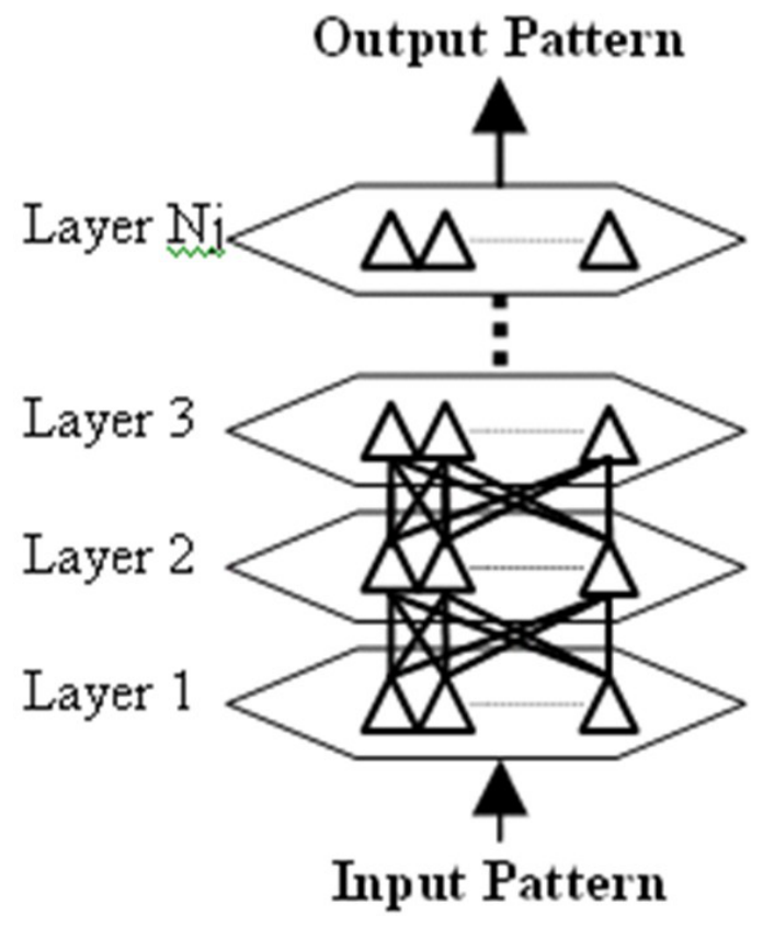
Considering (8) and (16), it is clear that the summation of nonlinear expressions and also the subtraction of linear expression from identity expression in the mapping relation of both two successive patterns were decreased K+1 times its corresponding value in the total mapping. On the other hand, neural networks having a smaller number of neurons with simpler structures can be found to operate as an almost identity operator. Therefore, with the similar number of sample neural networks for both successive patterns, a mapping can be found between the set of input and output patterns. The diagrams indicated in Figure 2 and Figure 3 show the architecture used in the MLP network.
After obtaining the coefficient matrices for each training neural network between two successive patterns, the coefficient matrix of output layer in each neural network is merged into the coefficient matrix of the input layer of the next neural network to create an MLP network.
However, it is difficult to use interval patterns according to definition (8) regarding time series because an output signal like is preferred to be modeled and finally predicted for the previous multi-signal set like (relation (1)). Nevertheless, some techniques can be used to equalize the dimension of the output pattern with the dimension of the input pattern. It should only be considered that signal is to be obtained from the output pattern at each time in this dimension increase, and the patterns should be defined in a way that the mapping between two patterns will not be more complicated than the mapping presented in (1). The method which was taken into account here was very simple. It was assumed that the output pattern was defined like for each input pattern like . The only difference is that the first member of the output pattern was signal which replaced yt-1 in the input pattern. Using the input and output patterns, the interval patterns can be defined according to (8).
4. Simulation
One of the applications of predicting time series is to predict solar storms. This phenomenon has a tangible impact on the weather. On the one hand, the radiation of cosmic ray resulting from solar storms influences the operations of satellites and telecommunications. For instance, the prediction of time series pertaining to this phenomenon was stimulated using the proposed method. The results were compared with some known methods. One of the common criteria used to determine the quality of predicting solar storms was to predict it in the method of a few steps forward between 1871 and 1881. In this study, the information pertaining to the annual solar storms between 1770 and 1870 was used to form patterns and train the network. The prediction results can be seen in Table 1 [53].
This table clearly indicates that prediction done in the interval patterns method resulted in fewer errors. Figure 3 indicates the results of prediction. In this method, 4 interval patterns (IP(4)) were used, and each neural network had 4 neurons in the hidden layer. IP(4) was finally used in a 5-layer MLP network. Using back propagation method, each layer was learnt. Symmetric sigmoid functions were used as the activating functions in each hidden layer. In the second layer, the linear activating functions were used. All the specifications of the above network were obtained by trial and error for the optimized state. The appropriate dimension was also detected for the regression vector in trial and error while considering . However, using result (7) in determining the minimum dimension also resulted in .
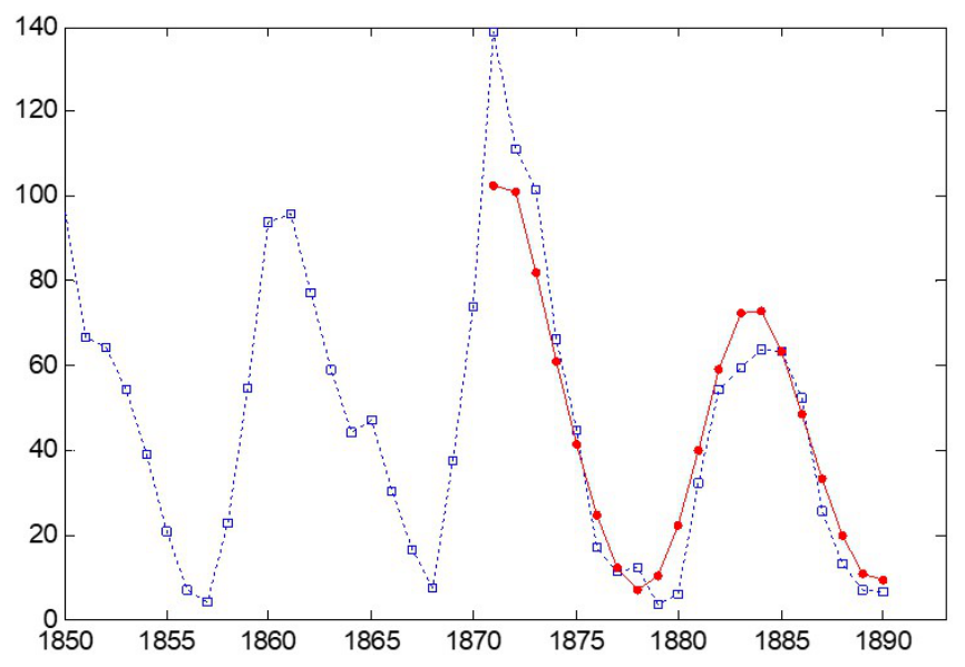
In the second part, simulation was done for the prediction of solar storms for 2 years forward between 1970 and 1889, in which several known methods of prediction were used. Table 2 indicates the results [54].

Table 1.
Comparing the Prediction Results of Some Known Methods in 11 Steps forward with the Interval Patterns Method.
Table 1.
Comparing the Prediction Results of Some Known Methods in 11 Steps forward with the Interval Patterns Method.
| Maximum Absolute Error | Root Mean Square Error | Prediction Horizon | Explain | Predictor |
|---|---|---|---|---|
| 81 | 32.6 | 11 | Autoregressive | AR[1] |
| 81 | 32.6 | 11 | Bilinear Predictor | BL[55] |
| 76 | 35 | 11 | - | SETAR[56] |
| 47 | 21.4 | 11 | Optimal Error Predictor | OEP[57,58] |
| 81 | 29.4 | 11 | - | GMDH[58,59] |
| 45 | 19.9 | 11 | Nonlinear Set Membership | NSM11[53] |
| 63 | 23.4 | 11 | Neural Network | NN11[53] |
| 31 | 12.7 | 11 | Interval Patterns | I P(4) |
As observed, the proposed method indicated better results. The criterion normalized mean square error, used as the comparison criteria in Table 2, is defined as follows:
Table 2.
Comparing the Results of Predicting Some Known Methods in 20 Steps forward in the Method of Interval Patterns.
Table 2.
Comparing the Results of Predicting Some Known Methods in 20 Steps forward in the Method of Interval Patterns.
| Normalized Mean Square Error | Prediction Horizon | Explain | Predictor |
|---|---|---|---|
| 0.252 | 20 | Autoregressive Moving Average | ARMA[1] |
| 0.348 | 20 | Specified Network Recurrent | Elman[54] |
| 0.115 | 20 | Finite Impulse Response | FIR[54] |
| 0.162 | 20 | Elman & FIR | Extended Elman[54] |
| 0.0957 | 20 | Interval Patterns | IP(4) |
In this criterion,, and refer to the observed information, their mean, and information resulting from prediction, respectively. The MLP network used to predict 20 steps forward is the same as the specifications of neural network used to predict 11 steps forward. The only difference was that the information pertaining solar storms between 1700 and 1869 was used here to create patterns and train the network. The result of this prediction can be seen in Figure 4.
Figure 4.
Prediction of 11 steps forward using the interval-pattern method.
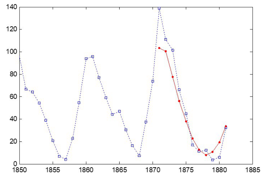
Figure 5.
Prediction of 20 steps forward using the interval-pattern method.
5. Conclusion
Pointing out the fact that many methods have been proposed to predict time series so far, a new architecture of the MPL neural network was introduced in this paper. In this architecture, layers were trained independently based on interval patterns which were defined with respect to the input and output patterns resulting from the information of time series. Therefore, a complicated and volatile mapping between two inputs and output patterns would turn into simple and identity mappings between successive patterns of the interval patterns, and the neural network would be trained simply and more efficiently. The minimum dimension which would be possible for a time series was also discussed. The prediction of some steps forward of solar storms was considered and compared with other known methods. The results clearly indicated the superiority of the proposed method.
References
- Box, G.E.P.; Jenkins, G.M.; Reinsel, G.C.; Ljung, G.M. Time Series Analysis: Forecasting and Control, 5 ed.; Wiley, 2015.
- Montgomery, D.C.; Jennings, C.L.; Kulahci, M. Introduction to Time Series Analysis and Forecasting, 2 ed.; Wiley, 2015.
- Makhoul, J. Linear Prediction: A Tutorial Review. Proceedings of the IEEE 1975, 63, 561–580. [CrossRef]
- Kim, H.J.; Lee, W.D.; Yang, H.S. A Modified FIR Network for Time Series Prediction. In Proceedings of the Proceedings of the 9th International Conference on Neural Information Processing, 2002, Vol. 5, pp. 2597–2600. [CrossRef]
- Eltoft, T.; de Figueiredo, R.J.P. Dynamical-Functional Neural Networks for Time Series Prediction. In Proceedings of the Proceedings of the International Joint Conference on Neural Networks, 1999, Vol. 4, pp. 2576–2579.
- Parcollet, T.; Morchid, M.; Linares, G.; De Mori, R. Quaternion Neural Networks for Spoken Language Understanding. In Proceedings of the 2016 IEEE Spoken Language Technology Workshop (SLT), 2016.
- Che, Z.; Purushotham, S.; Cho, K.; Sontag, D.; Liu, Y. Recurrent Neural Networks for Multivariate Time Series with Missing Values. Scientific Reports 2018, 8, 6085. [CrossRef]
- Rezaee, A. Using Genetic Algorithms for Designing of FIR Digital Filters. ICTACT Journal on Soft Computing 2010, 1, 18–22. [CrossRef]
- Tatar, A.; Barati-Harooni, A.; Najafi-Marghmaleki, A.; Norouzi-Firouz, H. Prediction of Reservoir Brine Properties Using Radial Basis Function (RBF) Neural Network. Petroleum 2015, 1, 349–357. [CrossRef]
- Kwin, C.T.; Yang, J.H.; Lee, E.W.; Choi, S.H. Rainfall-Runoff Modeling Using Dynamic Evolving Neural Fuzzy Inference System with Online Learning. Procedia Engineering 2016, 154, 1103–1109. [CrossRef]
- Hochreiter, S.; Schmidhuber, J. Long Short-Term Memory. Neural Computation 1997, 9, 1735–1780. [CrossRef]
- Cho, K.; van Merriënboer, B.; Gulcehre, C.; Bahdanau, D.; Bougares, F.; Schwenk, H.; Bengio, Y. Learning Phrase Representations using RNN Encoder–Decoder for Statistical Machine Translation. In Proceedings of the Proceedings of EMNLP, 2014, pp. 1724–1734.
- Bai, S.; Kolter, J.Z.; Koltun, V. An Empirical Evaluation of Generic Convolutional and Recurrent Networks for Sequence Modeling. arXiv preprint arXiv:1803.01271 2018.
- Salinas, D.; Flunkert, V.; Gasthaus, J.; Januschowski, T. DeepAR: Probabilistic Forecasting with Autoregressive Recurrent Networks. International Journal of Forecasting 2020, 36, 1181–1191. [CrossRef]
- Rangapuram, S.S.; Seeger, M.W.; Gasthaus, J.; Stella, L.; Wang, Y.; Januschowski, T. Deep State Space Models for Time Series Forecasting. In Proceedings of the Advances in Neural Information Processing Systems, 2018, Vol. 31.
- Oreshkin, B.N.; Carpov, D.; Chapados, N.; Bengio, Y. N-BEATS: Neural Basis Expansion Analysis for Interpretable Time Series Forecasting. In Proceedings of the International Conference on Learning Representations, 2020.
- Lim, B.; Arik, S.O.; Loeff, N.; Pfister, T. Temporal Fusion Transformers for Interpretable Multi-Horizon Time Series Forecasting. International Journal of Forecasting 2021, 37, 1748–1764. [CrossRef]
- Zhou, H.; Zhang, S.; Peng, J.; Zhang, S.; Li, J.; Xiong, H.; Zhang, W. Informer: Beyond Efficient Transformer for Long Sequence Time-Series Forecasting. In Proceedings of the Proceedings of the AAAI Conference on Artificial Intelligence, 2021, Vol. 35, pp. 11106–11115. [CrossRef]
- Wu, H.; Xu, J.; Wang, J.; Long, M. Autoformer: Decomposition Transformers with Auto-Correlation for Long-Term Series Forecasting. In Proceedings of the Advances in Neural Information Processing Systems, 2021, Vol. 34.
- Zhou, T.; Ma, Z.; Wen, Q.; Wang, X.; Sun, L.; Jin, R. FEDformer: Frequency Enhanced Decomposed Transformer for Long-Term Series Forecasting. In Proceedings of the Proceedings of the 39th International Conference on Machine Learning, 2022, Vol. 162, pp. 27268–27286.
- Liu, S.; Yu, H.; Liao, C.; Li, J.; Lin, W.; Liu, A.X.; Dustdar, S. Pyraformer: Low-Complexity Pyramidal Attention for Long-Range Time Series Modeling and Forecasting. In Proceedings of the International Conference on Learning Representations, 2022.
- Nie, Y.; Nguyen, N.H.; Sinthong, P.; Kalagnanam, J. A Time Series is Worth 64 Words: Long-Term Forecasting with Transformers. In Proceedings of the International Conference on Learning Representations, 2023.
- Wu, H.; Hu, T.; Liu, Y.; Zhou, H.; Wang, J.; Long, M. TimesNet: Temporal 2D-Variation Modeling for General Time Series Analysis. In Proceedings of the International Conference on Learning Representations, 2023.
- Zeng, A.; Chen, M.; Zhang, L.; Xu, Q. Are Transformers Effective for Time Series Forecasting? In Proceedings of the Proceedings of the AAAI Conference on Artificial Intelligence, 2023, Vol. 37, pp. 11121–11128. [CrossRef]
- Lim, B.; Zohren, S. Time-Series Forecasting with Deep Learning: A Survey. Philosophical Transactions of the Royal Society A 2021, 379, 20200209. [CrossRef]
- Ismail Fawaz, H.; Forestier, G.; Weber, J.; Idoumghar, L.; Muller, P.A. Deep Learning for Time Series Classification: A Review. Data Mining and Knowledge Discovery 2019, 33, 917–963. [CrossRef]
- Taylor, S.J.; Letham, B. Forecasting at Scale. The American Statistician 2018, 72, 37–45. [CrossRef]
- Kuremoto, T.; Kimura, S.; Kobayashi, K.; Obayashi, M. Time Series Forecasting Using a Deep Belief Network with Restricted Boltzmann Machines. Neurocomputing 2014, 137, 47–56. [CrossRef]
- Liu, M.; Zeng, A.; Chen, M.; Xu, Z.; Lai, Q.; Ma, L.; Xu, Q. SCINet: Time Series Modeling and Forecasting with Sample Convolution and Interaction. In Proceedings of the Advances in Neural Information Processing Systems, 2022, Vol. 35.
- Wu, N.; Green, B.; Ben, X.; O’Banion, S. Deep Transformer Models for Time Series Forecasting: The Influenza Prevalence Case. arXiv preprint arXiv:2001.08317 2020.
- Wen, R.; Torkkola, K.; Narayanaswamy, B.; Madeka, D. A Multi-Horizon Quantile Recurrent Forecaster. arXiv preprint arXiv:1711.11053 2017.
- Barzamini, R.; Hajati, F.; Gheisari, S.; Motamadinejad, M. Short term load forecasting using multi-layer perception and fuzzy inference systems. Journal of Applied Sciences 2012, 12, 40–47. [CrossRef]
- Fiorini, S.; Hajati, F.; Barla, A.; Girosi, F. Predicting diabetes second-line therapy initiation in the Australian population via timespan-guided neural attention network. PLOS ONE 2019, 10, e0211844.
- Tavakolian, A.; Hajati, F.; Rezaee, A.; Fasakhodi, A.O.; Uddin, S. Fast COVID-19 versus H1N1 screening using optimized parallel inception. Expert Systems with Applications 2022, 204, 117551. [CrossRef]
- Tavakolian, A.; Rezaee, A.; Hajati, F.; Uddin, S. Hospital readmission and length-of-stay prediction using an optimized hybrid deep model. Future Internet 2023, 15, 304. [CrossRef]
- Zobeiri, A.; Rezaee, A.; Hajati, F.; Argha, A.; Alinejad-Rokny, H. Post-cardiac arrest outcome prediction using machine learning: a systematic review and meta-analysis. International Journal of Medical Informatics 2025, 193, 105659. [CrossRef]
- Hajati, F.; Faez, K.; Pakazad, S.K. An Efficient Method for Face Localization and Recognition in Color Images. In Proceedings of the Systems, Man and Cybernetics, 2006. SMC’06. IEEE International Conference on. IEEE, 2006, Vol. 5, pp. 4214–4219. [CrossRef]
- Pakazad, S.K.; Faez, K.; Hajati, F. Face Detection Based on Central Geometrical Moments of Face Components. In Proceedings of the Systems, Man and Cybernetics, 2006. SMC’06. IEEE International Conference on, 2006, pp. 4225–4230.
- Hajati, F.; Raie, A.A.; Gao, Y. Pose-invariant 2.5 D face recognition using geodesic texture warping. In Proceedings of the 2010 11th International Conference on Control Automation Robotics & Vision. IEEE, 2010, pp. 1837–1841.
- Ayatollahi, F.; Raie, A.A.; Hajati, F. Expression-invariant face recognition using depth and intensity dual-tree complex wavelet transform features. Journal of Electronic Imaging 2015, 24, 023031–023031. [CrossRef]
- Shojaiee, F.; Hajati, F. Local composition derivative pattern for palmprint recognition. In Proceedings of the 2014 22nd Iranian Conference on Electrical Engineering (ICEE). IEEE, 2014, pp. 965–970.
- Abdoli, S.; Hajati, F. Offline signature verification using geodesic derivative pattern. In Proceedings of the 2014 22nd Iranian Conference on Electrical Engineering (ICEE). IEEE, 2014, pp. 1018–1023.
- Hajati, F.; Cheraghian, A.; Gheisari, S.; Gao, Y.; Mian, A.S. Surface geodesic pattern for 3D deformable texture matching. Pattern Recognition 2017, 62, 21–32. [CrossRef]
- Cremers, D.; Reid, I.; Saito, H.; Yang, M.H. Computer Vision–ACCV 2014: 12th Asian Conference on Computer Vision, Singapore, Singapore, November 1-5, 2014, Revised Selected Papers, Part V; Springer, 2015.
- Wang, S.; Lu, H.; Khan, A.; Hajati, F.; Khushi, M.; Uddin, S. A machine learning software tool for multiclass classification. Software Impacts 2022, 13, 100383. [CrossRef]
- Khan, M.W.; Sheng, H.; Zhang, H.; Du, H.; Wang, S.; Coroneo, M.; Hajati, F.; Shariflou, S.; Kalloniatis, M.; Phu, J.; et al. RVD: a handheld device-based fundus video dataset for retinal vessel segmentation. In Proceedings of the NeurIPS, 2024.
- Jamshidiha, S.; Rezaee, A.; Hajati, F.; Golzan, M.; Chiong, R. An explainable transformer model for Alzheimer’s disease detection using retinal imaging. Scientific Reports 2025, 15, 26773. [CrossRef]
- Barolli, L.; Takizawa, M.; Enokido, T.; Chen, H.C.; Matsuo, K. Advances on Broad-Band Wireless Computing, Communication and Applications: Proceedings of the 15th International Conference on Broad-Band and Wireless Computing, Communication and Applications (BWCCA-2020); Springer Nature, 2020.
- Mohamadzade, B.; Rezaee, A. Compact and broadband dual sleeve monopole antenna for GSM, WiMAX and WLAN application. Microwave and Optical Technology Letters 2017, 59, 1271–1277. [CrossRef]
- Rezaee, A. Model predictive for Mobile robot control. Transactions on environment and electrical engineering 2017, 2, 17–22. [CrossRef]
- Gavagsaz, E.; Rezaee, A.; Haj Seyyed Javadi, H. Load balancing in reducers for skewed data in MapReduce systems by using scalable simple random sampling. The Journal of Supercomputing 2018, 74, 3415–3440. [CrossRef]
- Sarvghad, S.; Rezaee, A.; Masomi, F. On the Relationship between Thinking Styles and Self-Efficacy of Pre-University Students in Shiraz 2011.
- Novara, C.; Milanese, M. Set Membership Prediction of Nonlinear Time Series. In Proceedings of the Proceedings of the 40th IEEE Conference on Decision and Control, 2001, pp. 1655–1660.
- Cholewo, T.J.; Zurada, J.M. Sequential Network Construction for Time Series Prediction. In Proceedings of the Proceedings of the International Conference on Neural Networks, 1997, Vol. 4, pp. 2034–2038.
- Granger, C.W.J.; Andersen, A.P. An Introduction to Bilinear Time Series Models; Vandenhoeck and Ruprecht: Göttingen, 1978.
- Tong, H.; Lim, K.S. Threshold Autoregression, Limit Cycles and Cyclical Data. Journal of the Royal Statistical Society: Series B 1980, 42, 245–292. [CrossRef]
- Milanese, M.; Tempo, R. Optimal Algorithms Theory for Estimation and Prediction. IEEE Transactions on Automatic Control 1985, 30, 730–738. [CrossRef]
- Vicino, A.; Tempo, R.; Genesio, R.; Milanese, M. Optimal Error and GMDH Predictors. International Journal of Forecasting 1987, 3, 313–328. [CrossRef]
- Ivakhnenko, A.G. Heuristic Self-Organization in Problems of Engineering Cybernetics. Automatica 1970, 6, 207–219. [CrossRef]
Figure 1.
Displaying interval patterns on 5D input and output patterns.
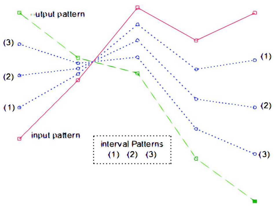
Figure 2.
Training diagram of each layer for training two successive patterns.
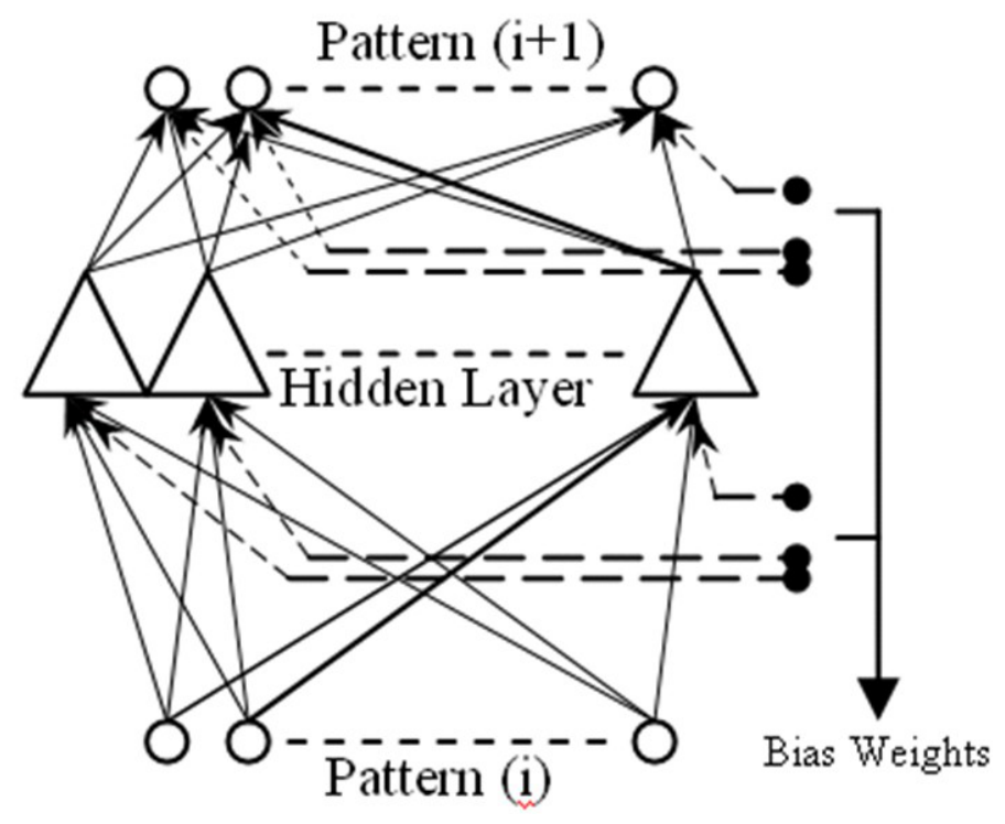
Figure 3.
The final diagram of the MLP network.
Disclaimer/Publisher’s Note: The statements, opinions and data contained in all publications are solely those of the individual author(s) and contributor(s) and not of MDPI and/or the editor(s). MDPI and/or the editor(s) disclaim responsibility for any injury to people or property resulting from any ideas, methods, instructions or products referred to in the content. |
© 2026 by the authors. Licensee MDPI, Basel, Switzerland. This article is an open access article distributed under the terms and conditions of the Creative Commons Attribution (CC BY) license (http://creativecommons.org/licenses/by/4.0/).
Copyright: This open access article is published under a Creative Commons CC BY 4.0 license, which permit the free download, distribution, and reuse, provided that the author and preprint are cited in any reuse.