

Submitted:
15 August 2026
Posted:
18 August 2026
You are already at the latest version
Abstract
Background: Implant-prosthetic rehabilitation of single-tooth edentulism often requires orthodontic reshaping of the potential implant-prosthetic space because its dimensions change due to the migration of adjacent teeth. In this context, it is very important to understand the force system generated by orthodontic arches in order to control tooth movement and to achieve, at the end of orthodontic treatment, the correct dimensions of the potential implant-prosthetic space for dental implant placement. Materials and Methods: The study was based on a set of 658 CBCT images from a 25-year-old female patient with maxillary and mandibular lateral edentulism. The images were processed using InVesalius and Geomagic software for the three-dimensional reconstruction of bone, dental, and periodontal ligament structures. Orthodontic components, including brackets, adhesive, and round-section nickel-titanium wires with a diameter of 0.012 inches, were modeled in SolidWorks. Based on virtual measurements of the wire geometry and using the relationships from the Theory of Elasticity and Strength of Materials, the elastic forces and reactions at the bracket components were calculated. Results: The study revealed an uneven distribution of forces along the orthodontic arches. For the upper arch, the elastic force values ranged from 0.044 to 0.383 N, and for the lower arch, from 0.050 to 0.308 N. The calculated reactions at the bracket components also varied depending on the orthodontic archwire geometry and the position of the support points. Conclusions: Three-dimensional modeling based on CBCT data, combined with classical methods of mechanics, allows for a personalized assessment of the force system in an orthodontic appliance. The results confirm the major influence of archwire geometry and bracket positioning on mechanical stresses and provide a basis for the biomechanical optimization of pre-implant orthodontic treatment.
Keywords:
pre-prosthetic orthodontics
; three-dimensional modeling
; CBCT
; orthodontic biomechanics
; elastic forces
; bracket
; nickel-titanium archwire
1. Introduction
Implant-prosthetic rehabilitation of single-tooth edentulism is a functionally and aesthetically predictable solution, but its success depends essentially on a well-designed interdisciplinary (prosthetic and orthodontic) treatment plan. One of the determining factors for correct implant placement is the availability of adequate dimensions of the potential implant-prosthetic space—mesiodistally, vertically, and buccal-orally—so that the final restoration complies with the biomechanical, aesthetic, and biological principles of implant-supported prosthetic restoration [1,2].
In many clinical situations, early tooth loss is followed by migration of adjacent teeth, tooth tilting, changes in occlusal contacts, and a reduction in the space required for implant placement. In these cases, orthodontic treatment plays a fundamental role by realigning dental axes, converging or parallelizing the roots, and restoring the size of the edentulous space to a position favorable for prosthetic restoration [2,4]. Thus, orthodontics serves not only to “create space” but also to optimize the three-dimensional conditions for the implant, contributing to the correct positioning of the future prosthetic abutment and the final crown.
The importance of this stage is particularly heightened in the anterior regions, where aesthetic demands are high, and any discrepancy in position or volume can compromise the final result. The literature indicates that implants placed without adequate orthodontic preparation may be associated with difficulties in prosthetic emergence, gingival margin asymmetries, or compromises in the aesthetic contour of the restoration [1,2]. Conversely, through proper treatment sequencing, orthodontics facilitates implant placement in an area with sufficient space and favorable root relationships, reducing the risk of prosthetic and surgical complications.
Furthermore, in growing patients, the timing of implant placement must be carefully considered, as implants behave like ankylosed structures and do not follow the physiological growth of the jawbones. For this reason, in certain situations, orthodontic treatment also serves to maintain or reopen the space until skeletal maturity is reached, at which point implantation can be performed under conditions of long-term stability [3]. This stage is essential for preventing vertical discrepancies and for maintaining dentoalveolar harmony over time.
Consequently, the role of orthodontics in creating space for implants goes beyond simple dental alignment, integrating biological, functional, and aesthetic principles into an interdisciplinary treatment plan [4,5]. However, to successfully achieve these objectives, it is necessary to understand and precisely adhere to the system of orthodontic forces capable of moving the teeth to align and reshape the implant-prosthetic space in accordance with bone biology, without causing excessive bone resorption. Only in this way can the primary and secondary stability of the dental implant be guaranteed [6,7].
In this context, the aim of the present study is to evaluate the entire system of forces acting on metal bracket-type components in an orthodontic setup designed to reshape the potential implant-prosthetic space.
2. Materials and Methods
2.1. CBCT Imaging Data
This study was based on a set of CBCT images acquired at a specialized dental clinic on January 25, 2024, for a 25-year-old female patient presenting with maxillary and mandibular lateral edentulism. This study was approved by Decision No. 156/August 30, 2023, of the Ethics Committee and was conducted with the patient’s consent.
As part of the study, a geometric model of the tissues was created based on the set of CBCT (Cone Beam Computed Tomography) images. The data was processed using software that converts CBCT images into primary geometries for the constituent tissues using specific filters based on different shades of gray. The initial geometry, which consisted of a “point cloud,” was processed using techniques and methods specific to reverse engineering. Initially, this “point cloud” was transformed into a multitude of spatial triangular surfaces, which subsequently formed perfectly closed surfaces for the bone components (maxilla and mandible) and for the specific dentition. Using techniques specific to both Reverse Engineering and Direct Engineering, based on “offset” surfaces, models of the periodontal ligaments for each tooth were obtained.
The models were loaded, one by one, into a CAD (Computer-Aided Design) program, where they were aligned based on a common coordinate system and converted into virtual solids. Within the same software, the metal components for the orthodontic wires and bracket-type elements were modeled using techniques specific to Direct Engineering. These models were added to the models of the bone, tooth, and periodontal ligament components. Elastic deformations were measured on the orthodontic archwire models in the virtual environment. Based on specific equations from the field of Strength of Materials, the elastic forces were determined, followed by the reactions; finally, the entire system of forces acting on the bracket-type components was evaluated.
Figure 1 shows a screenshot from the CS 3D Imaging program for the set of tomographic images containing 658 CBCT images for the patient under study.
2.2. Orthodontic Materials
For the orthodontic assembly, we analyzed, from a dimensional perspective, Orthofocus-type orthodontic wires for the maxilla and mandible with a circular cross-section and a diameter of 0.012 inches (approx. 0.3 mm), as shown in Figure 2.
Similarly, the bracket-type elements shown in Figure 3 were studied.
2.3. Software Used
2.3.1. InVesalius
InVesalius is open-source research software used for the three-dimensional reconstruction of medical images obtained through computed tomography (CT) or magnetic resonance imaging (MRI). The software converts tomographic images into 3D models of the body’s anatomical tissues to better understand internal biological structures. The resulting 3D models are available in standard formats (such as STL, OBJ, or PLY) and can be used for virtual prototyping and 3D printing. The software is used for medical diagnosis, surgical planning, dentistry, research, education, veterinary medicine, and even in engineering for the virtual prototyping of medical devices. It was developed by the Renato Archer Information Technology Center (CTI) in Brazil (CTI, Campinas, Brazil) [i4].
2.3.2. Geomagic
Geomagic is a professional software program for reverse engineering, 3D scanning, and dimensional inspection, used in the medical, automotive, and aerospace industries. Geomagic enables the conversion of 3D scans—which initially consist of “point clouds”—into CAD models. The software enables the conversion of 3D scans into CAD models consisting of surfaces or solids, the reconstruction of a digital model from a physical part, the comparison of manufactured parts with the original CAD model, and the “cleaning and repair” of meshes such as STL, OBJ, etc. (3D Systems, Rock Hill, SC, USA) [i4], [t1].
2.3.3. SolidWorks
SolidWorks is a professional computer-aided design (CAD) program used to generate 3D models of components, assemblies, and technical documentation specific to mechanical engineering and industrial design. It also allows for virtual testing and simulations for strength analysis (Simulation module), kinematic analysis (Motion module), thermal analysis, vibration analysis, and fluid flow analysis (Flow module), as well as fatigue testing (Fatigue module) [i4], [t1].
This software uses methods specific to Direct Engineering and may contain specialized modules (Dassault Systèmes, Velizy-Villacoublay, France).
2.3.4. Microsoft Office Software Components
Microsoft Office is a suite of software modules developed by Microsoft, used for working with data, documents, presentations, and diagrams and charts.
The Microsoft Office suite was used to draft documents, organize, manage, and analyze data, as well as to implement formulas and perform repetitive calculations (Microsoft Corporation, Redmond, One Microsoft Way, 1, 98052, USA).
2.3.5. Artificial Intelligence (AI) Modules
These were used to explain terms, techniques, concepts, and methods, or to detail the advantages and disadvantages of certain software modules.
2.4. Hardware Systems
A Hewlett Packard Z2 workstation with the following technical specifications was used for 3D modeling:
- 13th-generation Intel® Core™ i9 processor;
- 64 GB DDR5-4800 RAM (4 x 16 GB);
- Graphics: NVIDIA RTX™ A4500 (20 GB dedicated GDDR6 memory), memory slots: 4 DIMM, internal storage: 1 TB HP Z Turbo Drive PCIe® NVMe™ TLC SSD;
- Graphics: Intel® UHD Graphics, memory and storage: 64 GB memory / 1 TB SSD storage;
- Processor: Intel® Core™ i9-13900K (up to 5.8 GHz, with Intel® Turbo Boost technology);
- 36 MB L3 cache, 24 cores, processor L3 cache: 36 MB, processor family:
- Operating system: Windows 11 Pro.
To generate charts and graphs and for computational data analysis, several desktop computers with the following technical specifications were used:
- Intel Core i3 processor with a clock speed of 3.7 GHz;
- 8 GB of RAM;
- 466 GB hard drive;
- 64-bit Windows 10 operating system.
For similar purposes, a Lenovo laptop was also used with the following technical specifications:
- Intel Core i5 processor with a clock speed of 2.9 GHz;
- 476 GB SSD;
- 930 GB hard drive;
- 16 GB RAM;
- 64-bit Windows 10 operating system.
2.5. Methods
2.5.1. Methods Specific to Medical Imaging
Medical imaging methods are investigative techniques that allow for the visualization of the body’s structures, tissues, and functions without (or with minimal) surgical intervention. They are very important for medical diagnosis, treatment guidance, and patient monitoring [8] [i4].
The main medical imaging methods are based on radiography (X-ray), computed tomography (CT or CBCT), magnetic resonance imaging (MRI), ultrasound, nuclear medicine, fluoroscopy, or angiography.
2.5.2. Methods of Elasticity Theory
The methods of Elasticity Theory constitute a set of mechanical and mathematical procedures used to analyze the behavior of bodies considered elastic (deformable solids) when subjected to a system of forces or other external actions [9,10,11].
2.5.3. Methods of Strength of Materials
The methods of strength of materials consist of a set of computational procedures, principles, and assumptions used to analyze the behavior of deformable solid bodies (plates, beams, bars, shafts) when they are subjected to a system of forces and moments [18,19].
2.5.4. Reverse Engineering Methods
Reverse engineering methods consist of a set of processes and techniques used to study an existing product, system, or software in order to understand its structure, operation, and design principles without access to the original documentation.
This study will utilize methods specific to mechanical engineering, which may be based on 3D scanning, manual measurements, CAD reconstruction, materials analysis, and physical disassembly. Analytical and functional methods may also be used, such as functional analysis, mathematical modeling, numerical simulation, benchmarking, or AI-based reverse engineering.
2.5.5. Direct Engineering Methods
Direct Engineering Methods (also known as Forward Engineering) refer to the set of techniques and methods used to design and build a system, starting from requirements or design briefs and gradually moving toward actual implementation. In practice, the process begins with an idea, leads to a model, and then to a final product.
Forward engineering is a system development process that begins with requirements and specifications, proceeds to the creation of conceptual and design models, and culminates in implementation, testing, and operation. It is the opposite of reverse engineering, which starts with an existing system.
In this study, these methods were used to model orthodontic wires and bracket-type elements.
2.6. Three-Dimensional Model of an Orthodontic System
2.6.1. Three-Dimensional Models of the Bony Components (Maxilla and Mandible)
The patient’s CBCT scans were imported into the InVesalius program. Figure 4 shows the program interface after importing the set of scans.
To obtain a primary “point cloud” geometry, the dental enamel (adult) filter was used, as shown in Figure 5.
Because the shades of gray in enamel-type dental tissues are similar to those of bone components, the model was imported into the Geomagic software for editing and processing. Figure 6 shows the Geomagic interface after importing the model from InVesalius as a “point cloud.” In the first phase, this software automatically transforms the “point cloud” into spatial triangular surfaces. Initially, this model contained 5,093,918 primary triangular surfaces.
This model also contains elements that are part of the dentition due to the similar densities of the tooth enamel. These components were manually removed using specific techniques. Figure 7 shows the steps involved in these removal operations for the anterior region.
Next, the left lateral dentition was removed; some of these steps are shown in Figure 8.
Next, various reverse engineering techniques were used to process the model; certain gaps were filled; non-conforming surfaces were identified and removed; finishing techniques were applied; and, finally, the number of elementary triangular surfaces was reduced to 24,198. Figure 9 illustrates some of these operations.
Finally, the models were imported into SolidWorks, where they were converted into virtual solids, as shown in Figure 10.
2.6.2. Three-Dimensional Models of the Dentition
To create the tooth models, the dental enamel filter in the InVesalius program was used, and the initial model shown in Figure 11 was generated.
Initially, the model contained 2,795,770 triangular element surfaces in Geomagic, as shown in Figure 12.
In the first step, the areas corresponding to the bone components were removed, as shown in Figure 13.
The steps for removing bone components continued, and Figure 14 shows some of them.
After applying several techniques for finishing, filling gaps, reducing the number of triangular faces, and eliminating non-conforming faces, the model shown in Figure 15 was obtained, which had 100,110 element faces.
Finally, the dental model was imported into SolidWorks, where it was automatically converted into virtual solids, as shown in Figure 16.
2.6.3. Three-Dimensional Models of Dental Ligaments
To generate the models of the dental ligaments, we started with the dentition model and used Offset surfaces applied to the entire model in Geomagic. Subsequently, the surfaces corresponding to the dental crown areas were removed, then filled using Fill techniques to obtain perfectly closed surfaces; finally, the models were imported into SolidWorks, where they were converted into virtual solids, as shown in Figure 17. The cavities corresponding to the contact surfaces with the dentition were subsequently created using CAD techniques.
2.6.4. Three-Dimensional Model of the Dento-Maxillary Apparatus of the Patient Under Study
Next, the models of the dentition and the dental ligaments were loaded into the Assembly module of SolidWorks, as shown in Figure 18.
The models are derived from the same set of CBCT images and, for this reason, have identical coordinate systems. Figure 19 shows the models and the six reference planes, three for each model.
To ensure that the models are in the correct position, the corresponding reference planes were aligned. Figure 20 shows the three alignment operations based on the coincidence of the planes.
The result of the plane alignment operation is shown in Figure 21.
In the context of the assembly, a volume subtraction operation was performed between the ligament and the teeth, resulting in the dental ligament cavities, as shown in Figure 22.
Next, in the SolidWorks Assembly module, the model of the two bone components was loaded. Similar operations were performed to align the reference planes for the models, as shown in Figure 23.
Next, two volume subtractions were performed between the bone components and the dentition and dental ligaments, resulting in the dental alveoli within the bone components, as shown in Figure 24.
2.6.5. Three-Dimensional Models of the Bracket-Type Components and the Orthodontic Adhesive
Next, the bracket-type components were modeled using CAD and direct engineering techniques. The following section details the steps involved in generating a model of a bracket for the mandibular incisors. The sketch shown in Figure 25 was drawn on one of the initial reference planes.
Since this is a symmetrical component, we chose to model an extruded solid with a midplane, as shown in Figure 26.
The sketch shown in Figure 27 was drawn in a reference plane perpendicular to the original one.
Using this sketch, the basic shape was cut out from the outside (Flip side to cut – enabled), as shown in Figure 28.
In the initial planes sketch from Figure 29 was drawn.
This sketch was used to add an extrusive plane using Mid Plane, as shown in Figure 30.
In the same plane sketch from Figure 31 was drawn.
Using the sketch, a cut was created using the Mid Plane option, as shown in Figure 32.
Next, a reference plane parallel to the initial one was defined, as shown in Figure 33.
In this plane sketches from Figure 34 were drawn.
With this sketches cutouts from Figure 35 were obtained.
Next, additional fillet shape were generated, as shown in Figure 36.
Next, a new reference plane was defined at a distance from the base of the bracket – type component, as shown in Figure 37.
Next, the sketch shown in Figure 38 was defined in this plane.
This sketch was used to create a new extruded shape, as shown in Figure 39.
This extruded shape was duplicated using a Linear Pattern command, and the resulting model is shown in Figure 40.
This shape was cut out using a surface located at a distance from the base of the bracket-type component, and the result is shown in Figure 41.
Using an outline taken from the sole of the pattern, the pattern was cut out from the outside, as shown in Figure 42.
To generate the orthodontic wire model, three points were drawn on the bracket component model (Figure 43).
Models of all bracket-type components were created using similar techniques (Figure 44). Mirroring techniques were also used for the symmetrical components.
To model the orthodontic adhesive, the contour of the bracket-type component’s base was copied and then extruded, as shown in Figure 45.
The bracket-type components were positioned on the corresponding teeth; Figure 46 shows, for example, their placement on a canine.
All bracket-type components were positioned in a similar manner with the adhesive, resulting in the model shown in Figure 47.
By applying a volume reduction between the adhesive models and each individual tooth, the final adhesive models were obtained.
2.6.6. Three-Dimensional Models of Orthodontic Wires
Next, using the points corresponding to the bracket-type components, a spline curve was drawn for the maxilla, as shown in Figure 48.
A circle with a diameter of 0.012 inches (approx. 0.3 mm) was drawn in a plane perpendicular to this curve, as shown in Figure 49.
Next, using a Sweep feature, the virtual solid modeling the orthodontic wire for the maxilla was defined (Figure 50).
Figure 51 shows the model of the orthodontic wire for the maxilla.
Similarly, the orthodontic wire for the mandible was also modelled (Figure 52).
2.7. Application of Techniques and Methods Specific to the Theory of Elasticity and Strength of Materials in Evaluating the Force System in the Orthodontic System Under Study
Introductory Theoretical Concepts
From the Strength of Materials and the Theory of Elasticity, it is known that a bar with a constant cross-section, supported at both ends and subjected to a force F, undergoes an elastic deformation s. This deformation is called deflection (Figure 53-a). Figure 53-b shows the equivalent model based on reactions.
An orthodontic archwire can be considered a bar with a constant cross-section. Furthermore, points A, B, and C can correspond to bracket-type components. We can thus map the model in Figure 2.52 onto the bracket-type elements on the orthodontic archwire. Now, the problem is to determine the elastic forces F and the reactions VA and VB.
It is also known that:
there is a functional relationship between the force F and the deflection s. This is:
(1)
where
F – elastic force;
k – elastic constant;
s – elastic deformation (deflection).
From the Principles of Strength of Materials and the Theory of Elasticity, the elastic force F can be calculated as follows:
where: s is the deflection of the bar;
F is the elastic force;
L is the length of the bar;
E is Young’s modulus (the modulus of elasticity of the orthodontic archwire);
I is the axial moment of inertia, and, in the case of a bar with a circular cross-section, it is:
where d is the diameter of the bar (in this case, the diameter of the orthodontic archwire).
From equations (1) and (2), the elastic constant k can be determined as follows:
If the elastic force F is known, the reactions VA and VB can be estimated as follows:
Table 1 shows how mathematical models are applied to the jaw.
Similarly, the mathematical models were adapted for the mandibular dentition, as shown in Table 2.
where: M1dr – right primary molar; M2dr – right secondary molar; P1dr – right primary premolar; P2dr – right secondary premolar; Cdr – right canine; I2dr – right secondary incisor; I1dr – right primary incisor; M1st – left primary molar; M2st – left second molar; P1st – left first premolar; P2st – left second premolar; Cst – left canine; I2st – left second incisor; I1st – left first incisor.
To determine the lengths L, a, b, and s, points of type A and B were connected by line segments; then, from points of type C, perpendiculars were drawn to the lines of type AB to highlight the arrows of type s, as illustrated for the orthodontic wire on the maxilla in Figure 54. Point A corresponds to M1dr, B corresponds to Cdr, and point C corresponds to I2dr.
For the maxillary orthodontic wire the lines are shown in Figure 55.
For the mandibular orthodontic wire these lines are shown in Figure 56.
Figure 57 illustrates how to measure the L-type length, that is, segment AB (M1dr - I2dr).
Figure 58 illustrates how to measure a length of type a, that is, the distance from point A (M1dr) to the foot of the perpendicular drawn from point C (Cdr).
To determine distances of type s, the length of the perpendicular drawn from point C (Cdr) to line AB (M1dr - I2dr) was measured, as shown in Figure 59.
b-type distances are calculated using the formula:
b=La
3. Results
3.1. Determination of the L, a, and S Distances by Measurement in the Virtual Environment on the Orthodontic Wire Curve
3.2. Determination of the Elastic and Reaction Forces Acting on Bracket-Type Components
To apply the mathematical formulas (2) through (6), it was necessary to also consider the values of d and E.
The diameter of the spring is 0.012 inches, or 0.3048 mm, so:
d = 0.0003048 m
The spring is made of a nickel-titanium alloy, known as nitinol. For this material, the modulus of elasticity is:
E = 34,500,000,000 Pa
4. Discussion
This study aimed to evaluate the system of forces acting within an orthodontic appliance through an integrated engineering and medical approach, based on three-dimensional modeling, virtual measurements, and the application of classical methods from the Theory of Elasticity and Strength of Materials. The results obtained are consistent with the general direction described in the specialized literature, according to which orthodontic biomechanics must be analyzed by correlating the geometry of the appliance, the material properties, and the biological response of the dento-periodontal structures [26,27].
An essential element of the study is the construction of the three-dimensional geometric model, derived from CBCT images of a real patient.
In this regard, the results are consistent with the studies by Kapila et al., as well as those by Scarfe and Farman, which show that CBCT offers major advantages in orthodontics by providing precise three-dimensional information about dento-skeletal relationships [28,29]. However, unlike these studies, which focus primarily on diagnosis and planning, the present study extends the use of CBCT to a personalized mechanical analysis, in which imaging data are transformed into a numerical model capable of estimating force distribution.
The integration of bone, dental, and periodontal ligament models into a common coordinate system ensured the spatial consistency of the assembly and enabled the precise positioning of orthodontic components modeled using direct engineering. This step is critical from an engineering standpoint, as any misalignment would lead to erroneous values for the deformations and, consequently, for the calculated forces. Compared to the idealized models used in classical analysis of orthodontic systems, the present approach has the advantage of preserving the anatomical specificity of the case, which increases the clinical relevance of the results [30,31].
Modeling orthodontic wires using spline-type trajectories, defined based on the actual position of the brackets, represents a significant advantage of this study. This choice is consistent with the ideas formulated by Burstone, who demonstrated the importance of geometric control of the wire and the positioning of force application points in achieving predictable biomechanical systems [32]. The main difference from classical approaches lies in the fact that here the wire curves are not merely theoretically assumed but reconstructed from the actual position of the brackets, which reduces reliance on idealized assumptions and makes the analysis more closely aligned with the clinical situation.
From a mechanical standpoint, orthodontic wires have been considered elastic elements with a constant cross-section, and the material’s behavior has been approximated as linearly elastic. This assumption is useful for comparisons and for basic mechanical interpretation; however, the literature shows that modern Ni-Ti wires exhibit superelastic behavior and a significant dependence on activation and stress history [33]. Miura et al.[34] demonstrated as early as in classical studies that the Ni-Ti alloy possesses clinically relevant superelastic properties, and Kusy showed that the properties of orthodontic wires vary significantly depending on composition, diameter, and conditions of use [35].
Therefore, the current model should be interpreted as a valid engineering approximation for comparative analysis, not as a complete description of the material’s actual behavior. Analysis of the results reveals a non-uniform distribution of forces along the orthodontic wires, in both the maxilla and the mandible. This result is consistent with the principles described by Burstone [32], according to which even small geometric changes can significantly alter the distribution of moments and forces. Furthermore, studies in orthodontic biomechanics emphasize that the efficiency of tooth movement depends not only on the magnitude of the force but also on its direction, duration, and point of application [36,37]. From this perspective, the non-uniform distribution observed in the present model confirms the sensitivity of the orthodontic system to the geometric configuration of the assembly.
It is important to note that the developed model does not include effects such as spring–bracket friction, nonlinear contact, the influence of the viscoelastic properties of periodontal ligaments, or biological adaptation over time. In the literature, these elements are recognized as important factors that can significantly alter the system’s actual response [38,39]. However, their simplification in the present study is justified by the need to obtain a clear, controllable, and interpretable model capable of highlighting the direct influence of geometry on the forces developed.
From a clinical perspective, the results are consistent with the classic observations of Reitan and Storey, who demonstrated that effective tooth movement is achieved through moderate, well-controlled forces, and that overloading can have undesirable biological effects [40,41]. In this regard, the present study provides a useful framework for understanding how appliance geometry influences mechanical loading and, consequently, for optimizing therapeutic design.
Through the complexity of the geometric model and the integration of classical engineering methods into a three-dimensional CAD environment, the study demonstrates the feasibility of a rigorous interdisciplinary approach capable of providing a solid foundation for further numerical or experimental developments. Compared to existing studies, the main contribution lies in the shift from a general description of orthodontic biomechanics to a customized analysis based on the patient’s actual geometry and direct virtual measurements.
5. Conclusions
Based on the research conducted in this study, the following main conclusions can be drawn.
A detailed three-dimensional model of the dento-maxillary system and the orthodontic appliance was developed, based on real CBCT imaging data and advanced methods of inverse and direct engineering.
The proposed methodology allows for a direct correlation between the actual geometry of orthodontic wires and the distribution of elastic forces, eliminating some of the geometric simplifications used in traditional approaches.
The application of methods from the Theory of Elasticity and Strength of Materials led to the quantitative determination of the forces and reactions acting on bracket-type components, highlighting the non-uniform nature of the mechanical stresses.
The results confirm that the distribution of forces in an orthodontic system is strongly dependent on the geometry of the archwire and the positioning of the components, an aspect of major engineering significance.
The study demonstrates the feasibility of using a rigorously engineered framework for the mechanical analysis of orthodontic systems, providing a solid theoretical foundation for extending the analysis to advanced numerical models.
Future research directions may include incorporating the nonlinear behavior of materials, analysis using other virtual methods, consideration of friction and archwire–bracket contact, as well as experimental validation of the obtained results.
In conclusion, this study contributes to strengthening engineering approaches in the field of orthodontics, demonstrating that the integration of three-dimensional modeling with classical mechanics methods is an effective tool for the analysis and optimization of orthodontic systems.
The study demonstrates that the integration of CBCT data with three-dimensional modeling and classical methods from the Theory of Elasticity and Strength of Materials allows for a rigorous evaluation of the force system developed within an orthodontic setup. The geometric model obtained through reverse engineering provided an accurate representation of the dento-maxillary structures and orthodontic components, ensuring the necessary conditions for a relevant mechanical analysis.
The results revealed an uneven distribution of forces along the orthodontic wires, determined by the geometric characteristics of the assembly and the positioning of the support points. Despite the simplifications made, the proposed methodology provides a solid foundation for understanding the relationship between the appliance’s geometry and the resulting mechanical stresses.
Therefore, the interdisciplinary approach used confirms the usefulness of three-dimensional CAD modeling in orthodontic biomechanical analysis and supports the development of further methods for numerical and experimental evaluation, with potential applications in optimizing individualized treatment.
Author Contributions
Conceptualization, A.S.R, D.L.P, G.B, and S.M.S.P; methodology D.L.P and S.M.S.P; software ,D.L.P.; validation, D.L.P, G.B. and S.M.S.P..; formal analysis, D.L.P. and S.M.S.P; investigation, A.S.R., S.M.S.P and G.B.; resources, A.S.R. and S.M.S.P.; data curation, D.L.P. and G.B.; writing—original draft preparation, A.S.R., D.L.P., G.B. and S.M.S.P; writing—review and editing, A,S,R, D.L.P., G.B. and S.M.S.P.; visualization, A,S,R, D.L.P., G.B. and S.M.S.P; supervision, D.L.P..; project administration, S.M.S.P..; funding acquisition, A.S.R.. All authors have read and agreed to the published version of the manuscript.
Funding
This research was supported by The Ministry of Investments and European Projects, through the Health Program, project DOCMED+, MySMIS code350696, funded by the European Social Fund Plus (ESF+).”).
Institutional Review Board Statement
The study was conducted in accordance with the Declaration of Helsinki, and approved by the Institutional Review Board (or Ethics Committee) of The University of Medicine and Pharmacy of Craiova (protocol code 156 from 30.08.2023).
Informed Consent Statement
Informed consent was obtained from all subjects involved in the study. Written informed consent has been obtained from the patient(s) to publish this paper.
Data Availability Statement
The original contributions presented in this study are included in the article. Further inquiries can be directed to the corresponding author.
Acknowledgments
During the preparation of this study, the author(s) used ChatGPT for the purposes generating some text. The authors have reviewed and edited the output and take full responsibility for the content of this publication.”.
Conflicts of Interest
The authors declare no conflicts of interest. The funders had no role in the design of the study; in the collection, analyses, or interpretation of data; in the writing of the manuscript; or in the decision to publish the results.
References
- Oesterle LJ, Cronin RJ Jr, Ranly DM. Maxillary implants and the growing patient. Int J Oral Maxillofac Implants. 1993;8(4):377-387.
- Brugnolo E, Mazzocco C, Cordioli G, Majzoub Z. Clinical and radiographic findings following placement of single-tooth implants in young patients: case reports. Int J Periodontics Restorative Dent. 1996;16(5):421-433.
- Thilander B, Odman J, Lekholm U. Orthodontic aspects of the use of oral implants in adolescents: a 10-year follow-up study. Eur J Orthod. 2001. [CrossRef]
- Proffit WR, Fields HW Jr, Larson B, Sarver DM. Contemporary Orthodontics. 6th ed. St. Louis: Elsevier; 2019.
- Misch CE. Contemporary Implant Dentistry. 3rd ed. St. Louis: Mosby Elsevier; 2008.
- Alfallaj H. (2020). Pre-prosthetic orthodontics. The Saudi Dental Journal, 32(1), 7–14. [CrossRef]
- Small B. W. (2011). Pre-prosthetic orthodontics for aesthetics and function in restorative dentistry. General Dentistry, 59(2), 91–94.
- Bennett, J. C., & McLaughlin, R. P. Fundamentals of Orthodontic Treatment Mechanics. Le Grande Publishing. pp. 43–50, 2019.
- Buciu, G., Tarnita, D.N., Popa, D.L., Lungu, M.A., Miritoiu, C., Ungureanu, A., Virtual and experimental studies on human walking. Virtual lower leg environment. Innovative design of a tibial nail, Applied Mechanics and Materials 657, pp. 770–774, 2014. [CrossRef]
- Calin, D., Tarniţă, D., Popa, D., Rosca, A., Tarnita, D. The 3D Virtual Model of a Classical Hip Joint Prosthesis, *Applied Mechanics and Materials*, vol. 826, pp. 161–166, 2013. [CrossRef]
- Calin, D.C., Tarniţă, D., Popa, D.L., Calafeteanu, D., Tarnita, D., Virtual Model and Simulation of the Normal and Affected Human Hip Joint, *Applied Mechanics and Materials*, vol. 823, pp. 167–172, 2016 . [CrossRef]
- Duta A., Popa D.L., Vintila D.D., Buciu G., Dina N.A., Ionescu A., Berceanu M.C., Calin D.C., An Experimental and Virtual Approach to Hip Revision Prostheses. Diagnostics, vol. 12, pp. 1952, 2022. [CrossRef]
- Duta, A., Buciu G., Tarnita, D., Vintila, D., A Personalized Three-Dimensional Model of a Patient Using CT Images, Proceedings of the International Conference on Mechanical Engineering (ICOME 2022), vol. 15, pp. 62, 2023.
- Duta, A., Popa, D.L., Vintila, D.D., Buciu, G., Dina, N.A., Ionescu, A., Berceanu, M.C., Calin, D.C., “An Experimental and Virtual Approach to Hip Revision Prostheses,” *Diagnostics*, vol. 12, no. 8, pp. 1952, 2022.
- Katta, M., Petrescu, S.-M.-S., Dragomir, L.P., Popescu, M.R., Voinea Georgescu, R., Țuculină, M.J., Popa, D.L., Duță, A., Diaconu, O.A., Dascălu, I.T., “Using the Finite Element Method to Determine the Odonto-Periodontal Stress for a Patient with Angle Class II Division 1 Malocclusion,” Diagnostics, vol. 13, no. 9, pp. 1567, 2023. [CrossRef]
- Petrescu S.-M.-S., Rauten A.-M., Popescu M., Popescu M. R., Popa D. L., Buciu G., Ciucă E.-M., Dudan T.-C., Bătăiosu M., Analysis of Extreme Thermal Variations in the Oral Cavity of a Patient with a Fixed Metallic Orthodontic Appliance Using the Finite Element Method, Bioengineering, vol. 12, no. 9, MDPI, pp. 901, 2025. [CrossRef]
- Petrescu S.-M-S., Rauten A.-M., Popescu M., Popescu M. R., Popa D. L., Ilie D., Duță A., Racilă L. D., Vintilă D. D., Buciu G., Assessment of Thermal Influence on an Orthodontic System Using the Finite Element Method, Bioengineering, vol. 11, no. 10, pp. 1002, MDPI, 2024. [CrossRef]
- Petrescu, S.-M.-S., Tuculina, M.J., Popa, D.L., Duta, A., Salan, A.I., Voinea Georgescu, R., Diaconu, O.A., Turcu, A.A., Mocanu, H., Nicola, A.G. et al., Modeling and Simulating an Orthodontic System Using Virtual Methods. Diagnostics, 12, pp. 1296. [CrossRef]
- Popa D. L., Dascalu I. T., Petrescu S. M. S., Duta A., Vintila D. D., Buciu G., The use of virtual direct and reverse engineering techniques for the reconstruction of an orthodontic system, Acta Technica Napocensis—Series: Applied Mathematics, Mechanics, and Engineering, vol. 68, no. 1 & 2, pp. 471–476, 2025.
- Popa, A.G., Botez, M.D., Buru, M.Ș., Besoiu, T.S., Marchiș, A.G., Bredean, L., Guide to Assignments in Strength of Materials (I), 2nd Edition, Revised and Expanded, UTPRESS, Cluj-Napoca, pp. 7–171, 2020.
- Popa, D.L., Buciu, G., Calin, D.C., Popkonstantinović, B., Poenaru, F., “CAD, CAE, and Rapid Prototyping Methods Applied in Orthopedics for Long Bones,” FME Transactions, Vol. 47, No. 2, pp. 279–286, 2019.
- Popa, D.L., Calin, D.C., Buciu, G., Virtual and experimental device for testing hip revision prostheses, IOP Conference Series: Materials Science and Engineering 997(1), 012086, 2020.
- Popa, D.L., Iliuta, D., Petrovici, I.L., A virtual approach to orthopedic systems based on implants and prostheses, IOP Conference Series: Materials Science and Engineering 997(1), 012087, 2020.
- Vătu, M., Vintila, D., Popa, D.L., “3D Virtual Skull Model Based on CT or MRI Images Used for Dental Simulations,” *Applied Mechanics and Materials*, Vol. 880, pp. 101–110, 2018.
- Vătu, M., Crăițoiu, M.M., Vintilă, D., Mercuț, V., Popescu, M.S., Scrieciu, M., Popa, D.. L., Determination of Resistance Forces from Mandibular Movements through Dynamic Simulation Using Kinematic Analysis and the Finite Element Method,Romanian Journal of Oral Rehabilitation, Vol. 10, Issue 1, pp. 20–28, 2018.
- Liao, Z., Chen, J., Li, W., Darendeliler, M. A., Swain, M., & Li, Q. (2016). Biomechanical investigation into the role of the periodontal ligament in optimizing orthodontic force: a finite element case study. Archives of Oral Biology, 66, 98–107. [CrossRef]
- Machado A. W. (2026). Orthodontic creative mechanics. Dental Press Journal of Orthodontics, 31(1), e26spe1, . [CrossRef]
- Kapila S, Conley RS, Harrell WE Jr. The current status of cone-beam computed tomography imaging in orthodontics. Dentomaxillofac Radiol. 2011;40(1):24-34.
- Scarfe WC, Farman AG. What is cone-beam CT and how does it work? Dent Clin North Am. 2008;52(4):707-730. [CrossRef]
- Abuabara A. (2007). Biomechanical aspects of external root resorption in orthodontic therapy. Medicina oral, patologia oral y cirugia bucal, 12(8),.
- Lindauer, S. J., & Rebellato, J. (1996). Biomechanical considerations for orthodontic treatment of adults. Dental Clinics of North America, 40(4), 811–836. 32. Burstone CJ. The mechanics of the segmented arch techniques. Angle Orthod. 1966;36(2):99–120. [CrossRef]
- Frias Cortez, M. A., Bourauel, C., Reichert, C., Jäger, A., & Reimann, S. (2022). Numerical and biomechanical analysis of orthodontic treatment of patients with recovered periodontal disease. 83(4), 255–268. [CrossRef]
- Miura F, Mogi M, Ohura Y, Hamanaka H. The super-elastic properties of Japanese NiTi alloy wire for use in orthodontics. Am J Orthod. 1986;90(1):1-10. [CrossRef]
- Kusy RP. A review of contemporary archwires: their properties and characteristics. Angle Orthod. 1997;67(3):197-208.
- Wu, J., Liu, Y., Zhang, J., Peng, W., & Jiang, X. (2018). Biomechanical investigation of orthodontic treatment planning based on orthodontic force measurement and the finite element method prior to implementation: A case study. Technology and Health Care: Official Journal of the European Society for Engineering and Medicine, 26(S1), 347–359. [CrossRef]
- Iwasaki, L. R., Covell, D. A., Jr, Frazier-Bowers, S. A., Kapila, S., Huja, S. S., & Nickel, J. C. (2015). Personalized and precision orthodontic therapy. Orthodontics & Craniofacial Research, 18 Suppl 1, 1–7. [CrossRef]
- Redlich, M., Shoshan, S., & Palmon, A. (1999). Gingival response to orthodontic force. American Journal of Orthodontics and Dentofacial Orthopedics: Official Publication of the American Association of Orthodontists, Its Constituent Societies, and the American Board of Orthodontics, 116(2), 152–158. [CrossRef]
- Ahmad, W., Liang, K., Xiong, J., Dai, J., Cao, J., & Xia, Z. (2024). Precision Orthodontic Force Simulation Using a Nodal Displacement-Based Archwire Loading Approach. International Journal for Numerical Methods in Biomedical Engineering, 40(12), e3889. [CrossRef]
- Reitan K. Clinical and histologic observations on tooth movement during and after orthodontic treatment. Am J Orthod. 1967;53(12):927-952.
- Storey E. The nature of tooth movement. Am J Orthod. 1973;63(3):292-314.
- [i1] https://invesalius.github.io/, accessed: May 4, 2025.
- [i2] http://www.geomagic.com/en, accessed: November 12, 2025.
- [i3] http://www3.agora.ro/index.php?qs_sect_id=936, SolidWorks, the complete 3D solution, Claudiu Bîrlogeanu, accessed July 2025;
- [i4] https://www.omniadental.ro/numerotarea-dintilor-in-stomatologie/, accessed May 2025.
- [t1] Geomagic, Tutorials, 2013–2026.
- [t2] SolidWorks, Tutorials, 1997–2026.
Figure 1.
CBCT images of the patient under study.
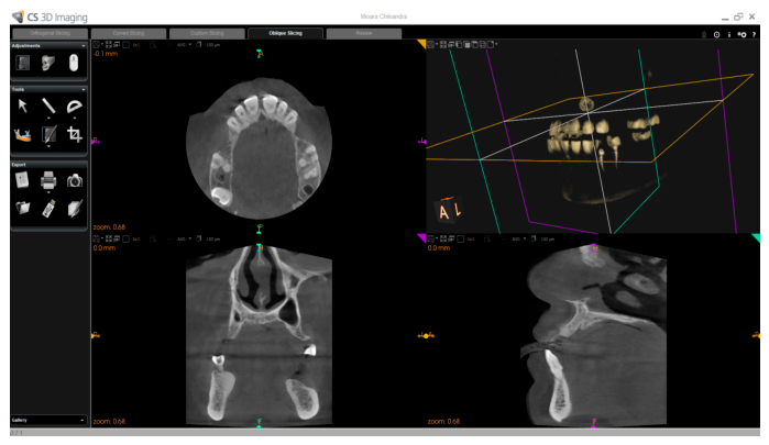
Figure 2.
Orthofocus Orthodontic Archwire Type.
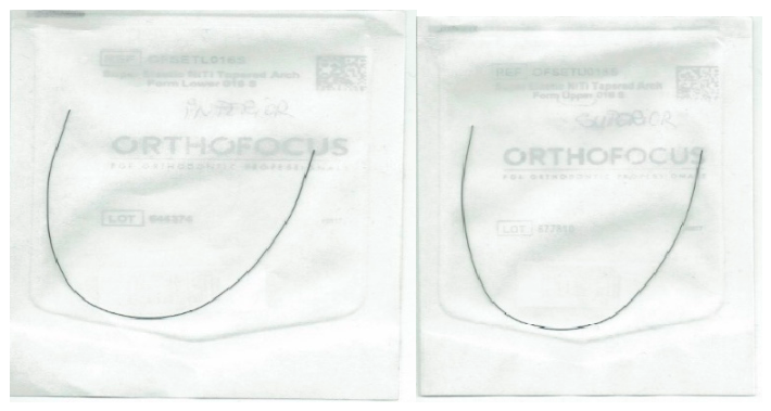
Figure 3.
Bracket-type elements.
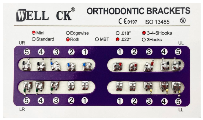
Figure 4.
Interface of the InVesalius Software.
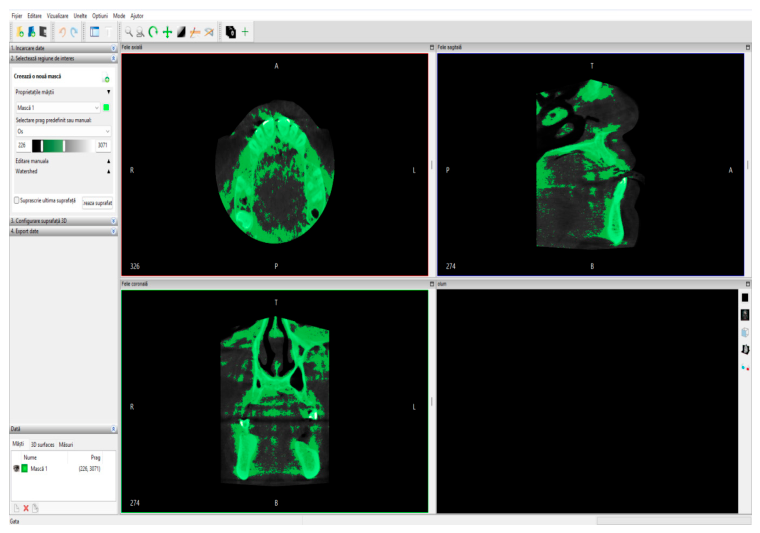
Figure 5.
Use of the dental enamel filter.
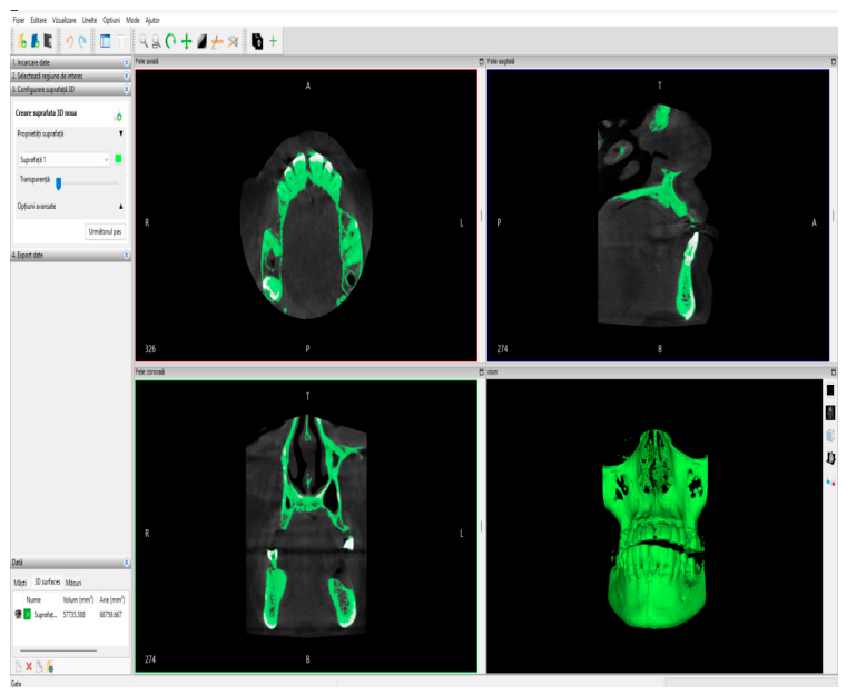
Figure 6.
The initial geometry of the model in the Geomagic Software.
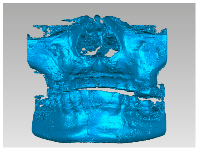
Figure 7.
Extraction of front teeth.
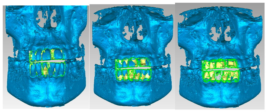
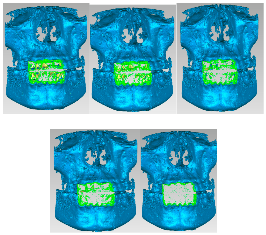
Figure 8.
Extraction of the lateral left dentition.
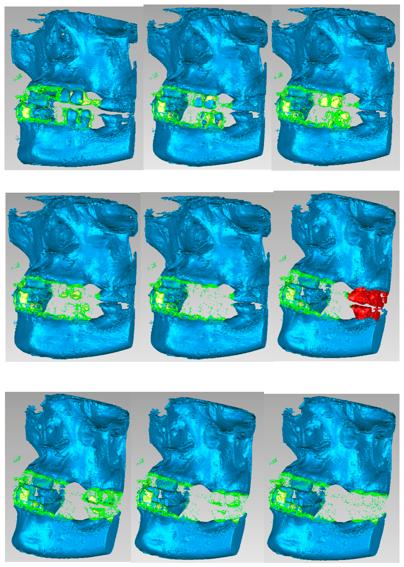
Figure 9.
Finalizing the models for the bone components.
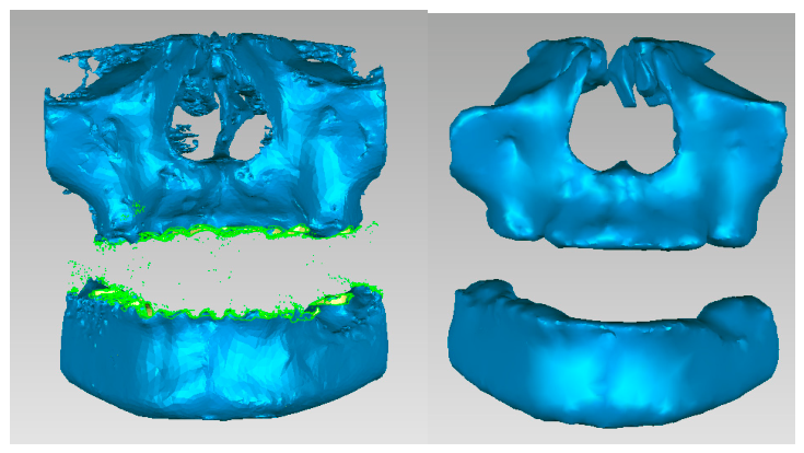
Figure 10.
Models imported in SolidWorks.
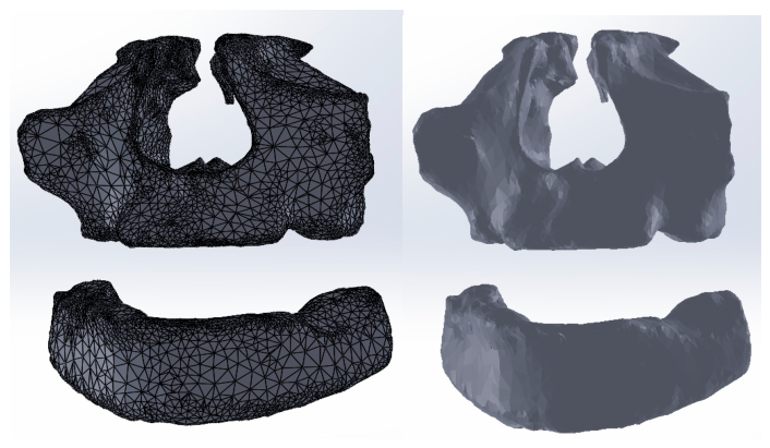
Figure 11.
Primary Model of the dentition in InVesalius.
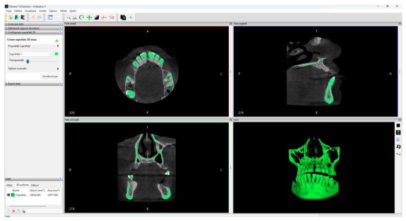
Figure 12.
Primary Model of the dentition in Geomagic.
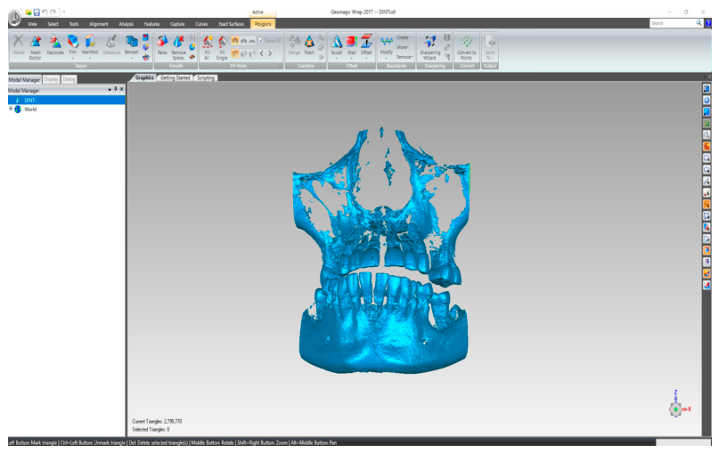
Figure 13.
Removal steps in Geomagic.
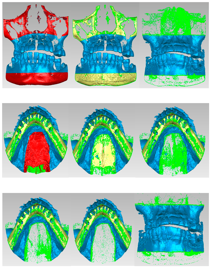
Figure 14.
Removal bone components in GeoMagic.
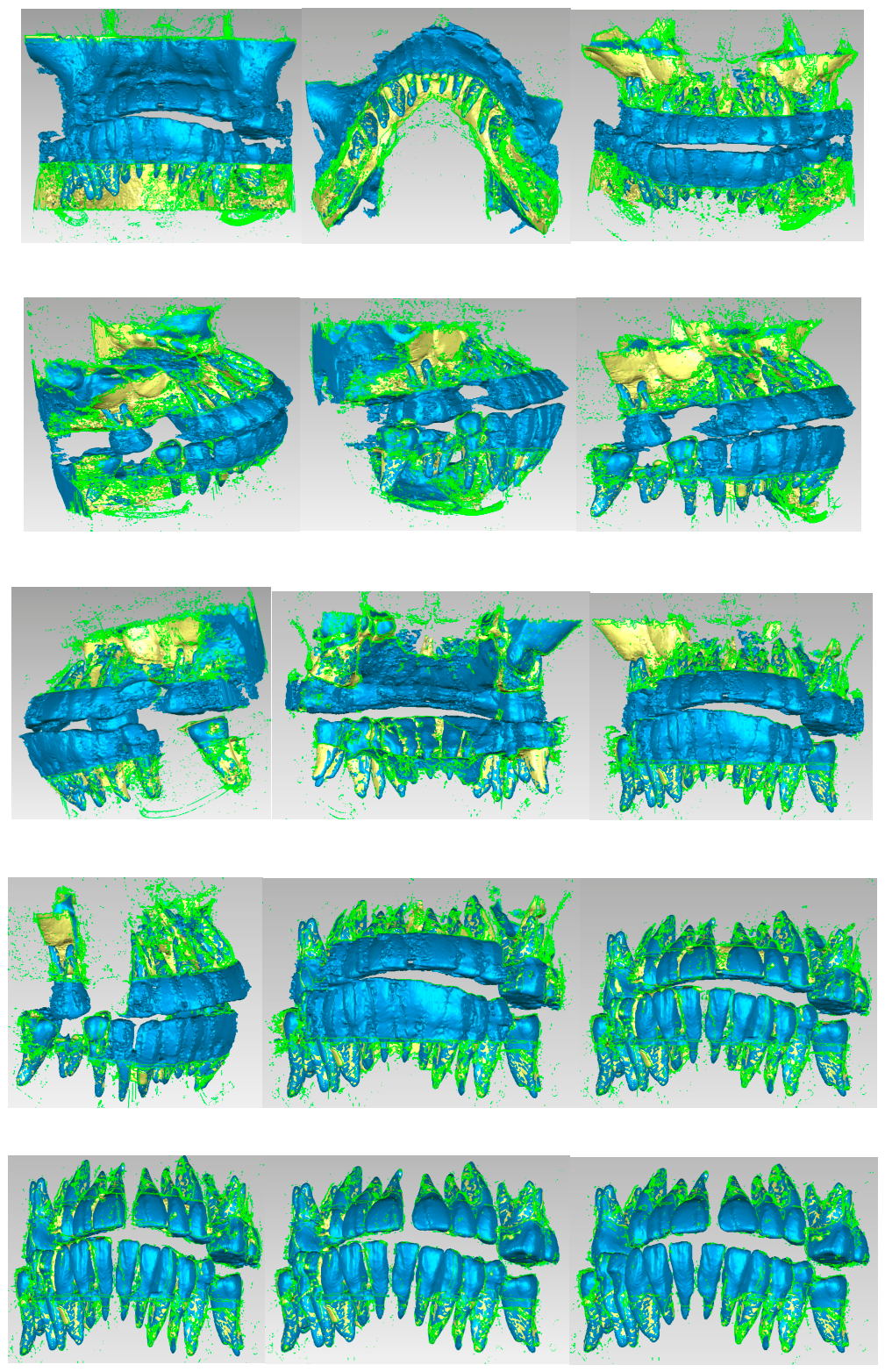
Figure 15.
Final Model of the dentition in GeoMagic.
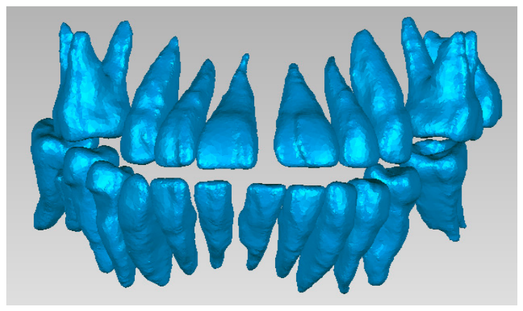
Figure 16.
Dental Model in SolidWorks.
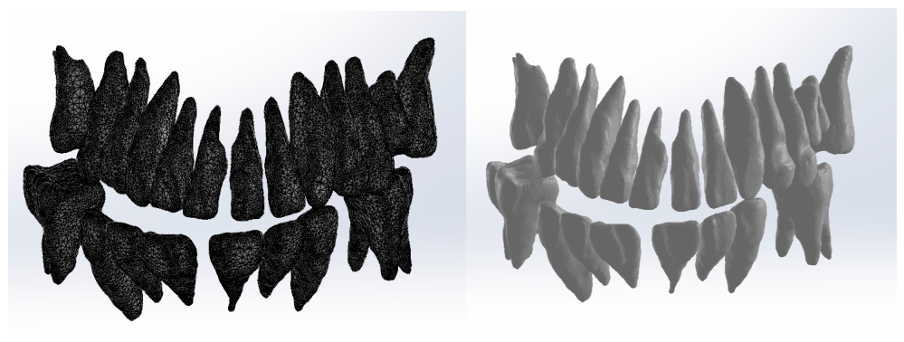
Figure 17.
The Initial Model of the Ligaments Imported in SolidWorks.
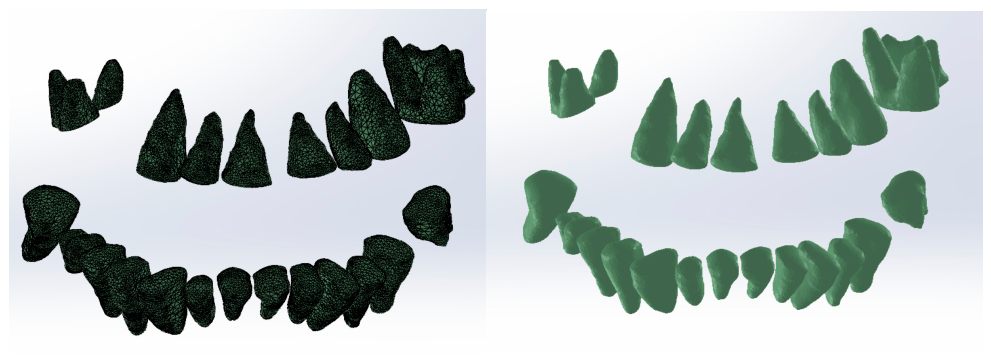
Figure 18.
Dental and ligaments models in the Assembly module.
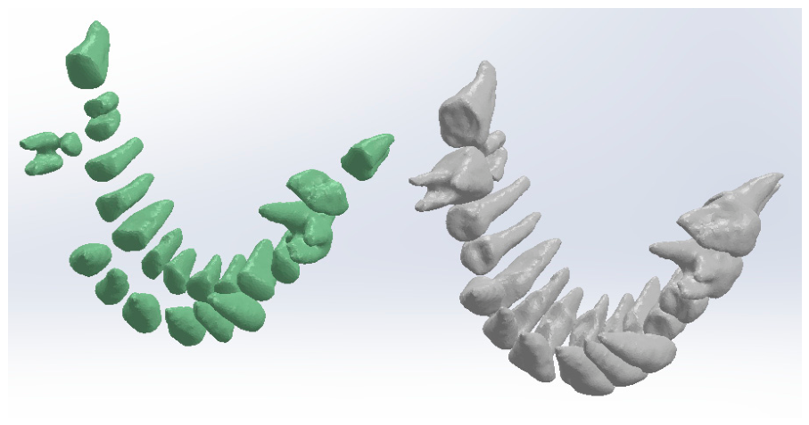
Figure 19.
Three-dimensional models in the six references plans.
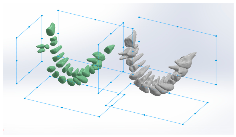
Figure 20.
Alignment of reference planes.
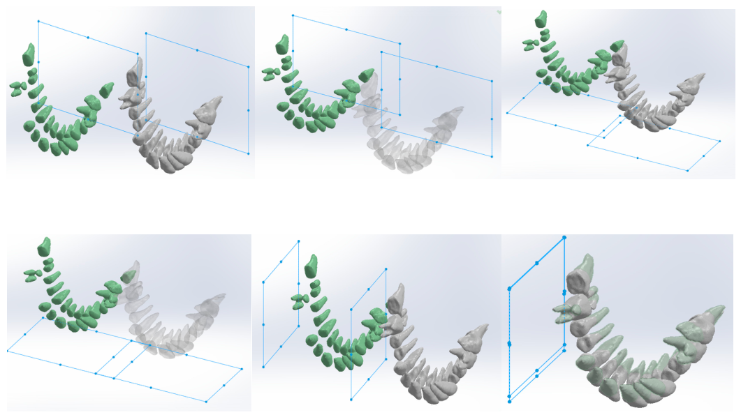
Figure 21.
The result of aligning in the reference planes.
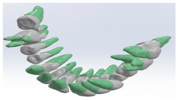
Figure 22.
The result of applying the volume subtraction.
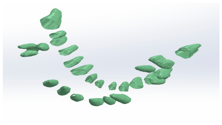
Figure 23.
Alignment of the reference planes for the bone components.

Figure 24.
Generating dental alveola in the two bone components.
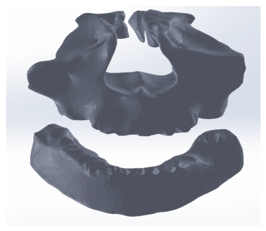
Figure 25.
Initial reference planes.
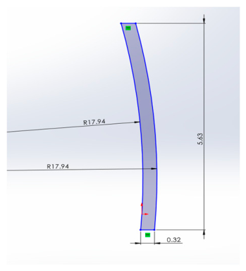
Figure 26.
Base form of the model.
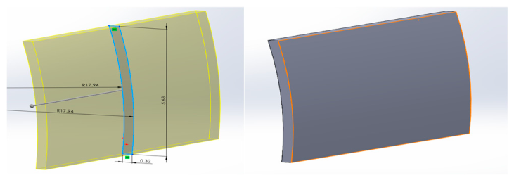
Figure 27.
Sketch drawn in a reference plane perpendicular to the original.
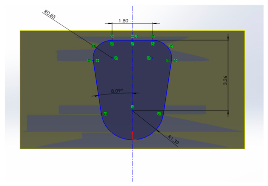
Figure 28.
Cut-off in the base form.
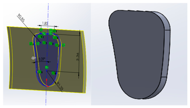
Figure 29.
Sketch of the initial plane.
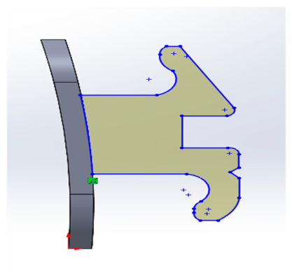
Figure 30.
Extruded shape.
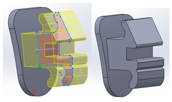
Figure 31.
Sketch drawn in the same plane.
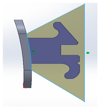
Figure 32.
Median cut.
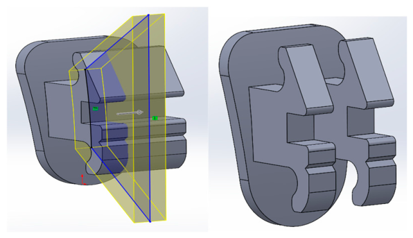
Figure 33.
Defining a reference plane.
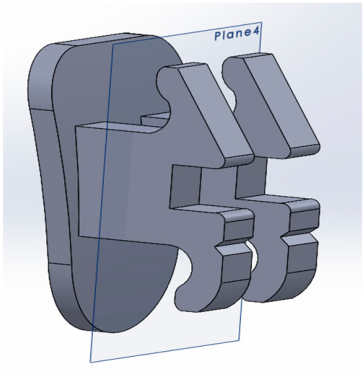
Figure 34.
Sketches in the defined plane.
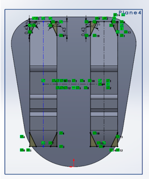
Figure 35.
Cutouts generated using the Cut-Extrude command.
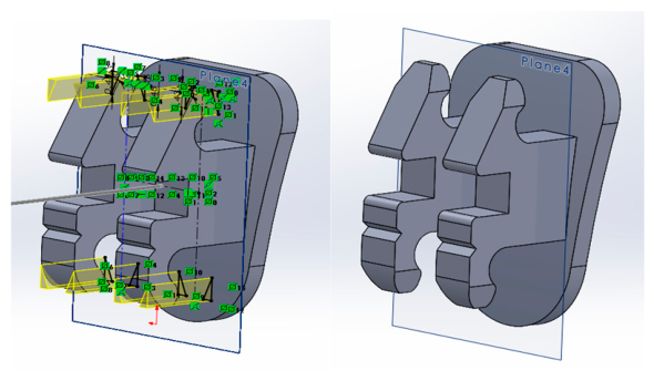
Figure 36.
Fillet shapes.
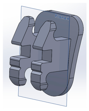
Figure 37.
Defining a reference plane.
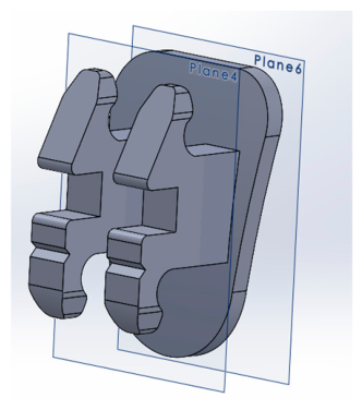
Figure 38.
Sketch in the new defined plane.
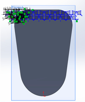
Figure 39.
Extruded shape.
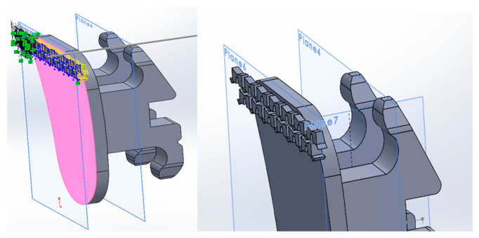
Figure 40.
Linear Pattern Multiplication.
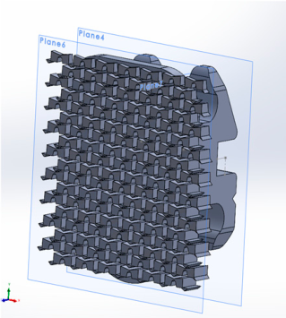
Figure 41.
Cutting – out the pattern type shape.
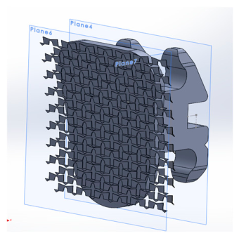
Figure 42.
Outline cutting.
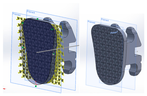
Figure 43.
Defining the three points along the orthodontic archwire path.
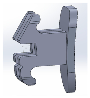
Figure 44.
Models of the bracket – type components used in the study.
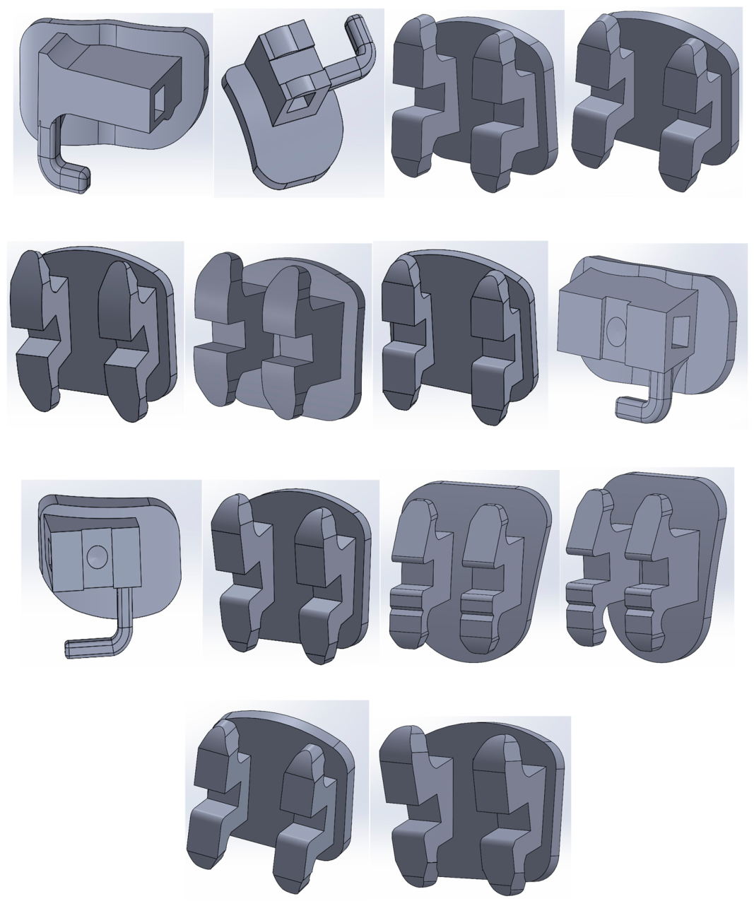
Figure 45.
The initial adhesive model.
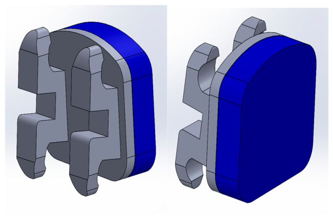
Figure 46.
Placement of the adhesive and bracket – type component on a canine tooth.
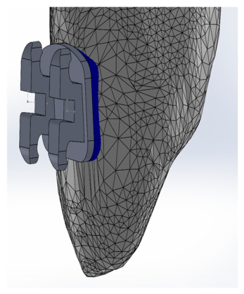
Figure 47.
Positioning of bracket – type components.
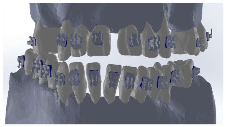
Figure 48.
Spline Curve for the jaw.
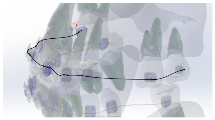
Figure 49.
A circle drawn in a plane perpendicular to the Spline Curve.
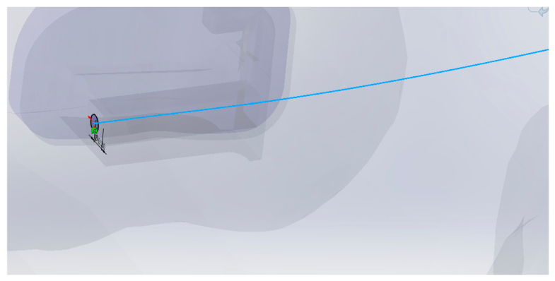
Figure 50.
The virtual solid modelling of the orthodontic maxillary wire.
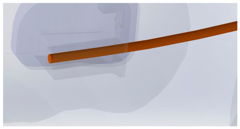
Figure 51.
Model of the upper orthodontic wire.
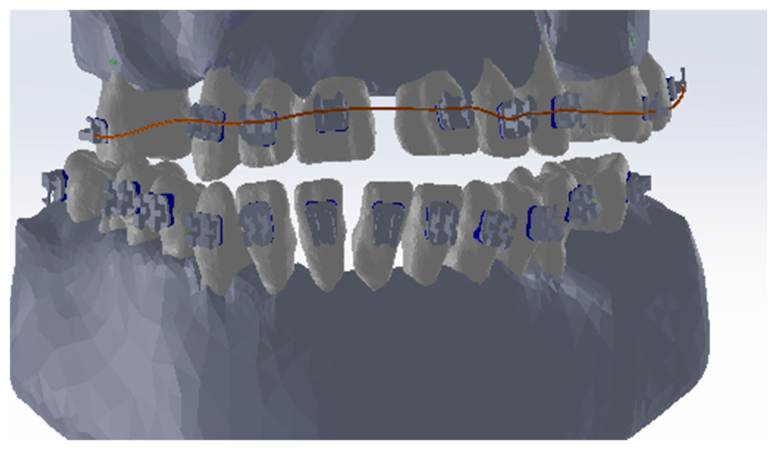
Figure 52.
Model of the orthodontic archwires.
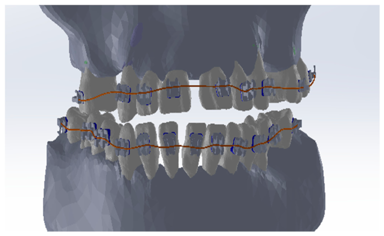
Figure 53.
The elastic force F that produces the deflection s (a—model with action forces; b—equivalent model with reaction forces).
Figure 53.
The elastic force F that produces the deflection s (a—model with action forces; b—equivalent model with reaction forces).
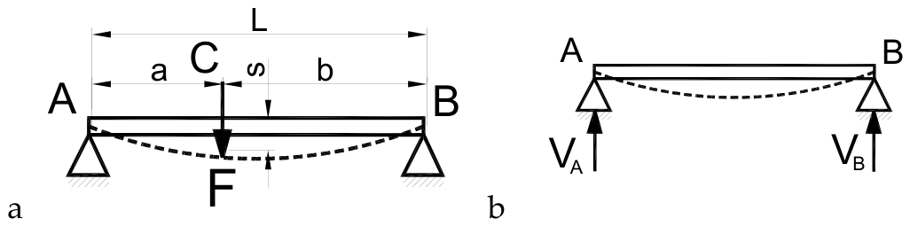
Figure 54.
Drawing the lines AB and the perpendiculars from C.
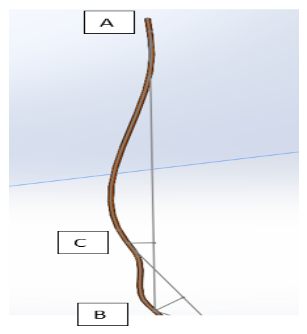
Figure 55.
Drawing the lines AB and the perpendicular from C for the upper orthodontic wire.
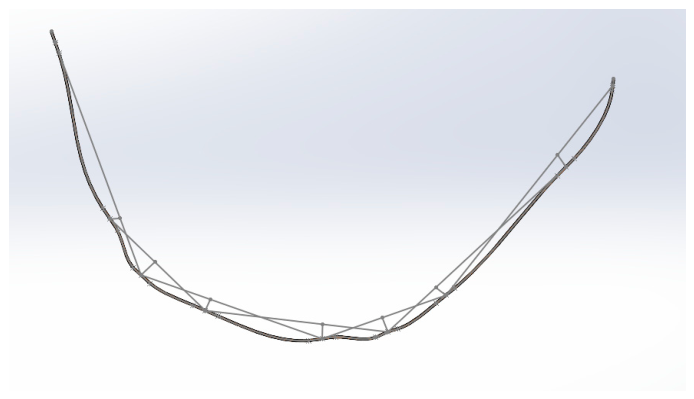
Figure 56.
Drawing the lines AB and the perpendicular from C for the lower orthodontic wire.
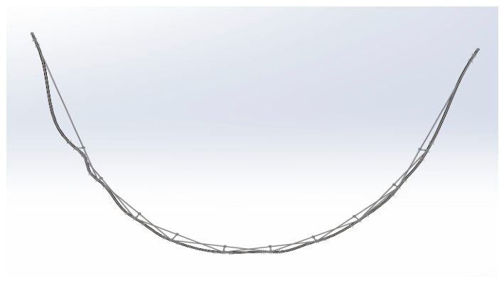
Figure 57.
Measuring the distance AB.
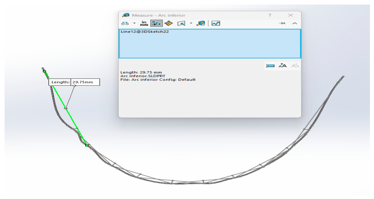
Figure 58.
Measurement of distance type a.
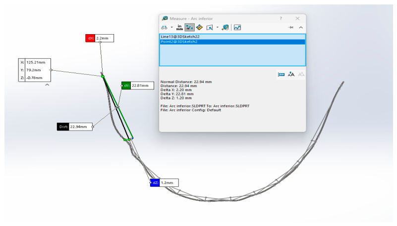
Figure 59.
Measurement of the s-type distance.
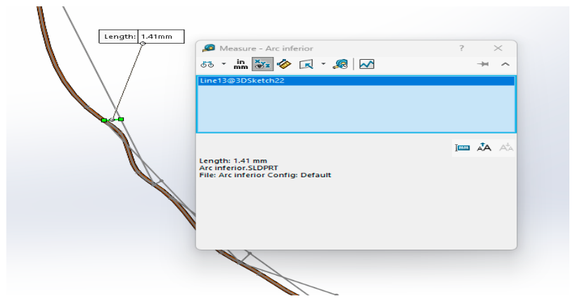
Figure 60.
Forces acting on the upper wire.
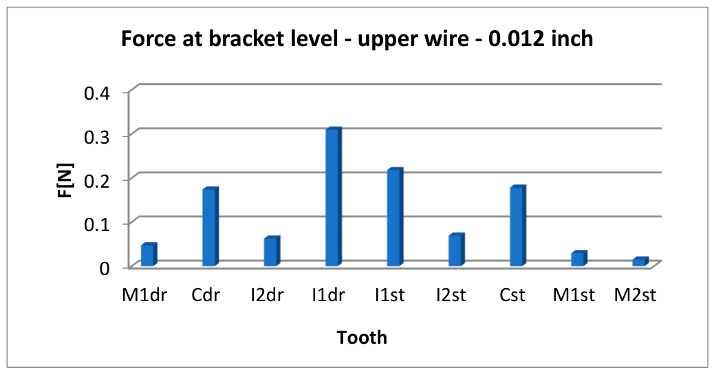
Figure 61.
Forces acting on the lower wire.
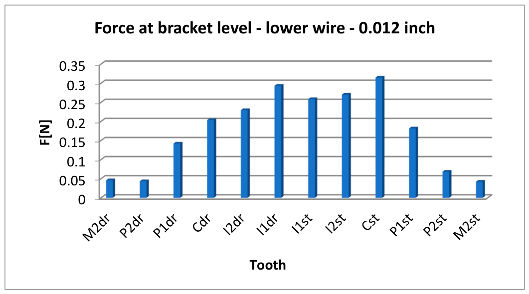

Table 1.
Mathematical models applied to the jaw.
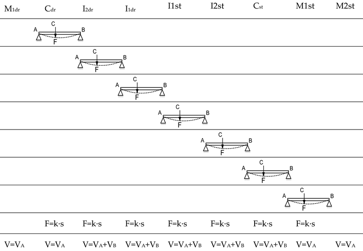 |
Table 2.
Mathematical models applied to the mandible.
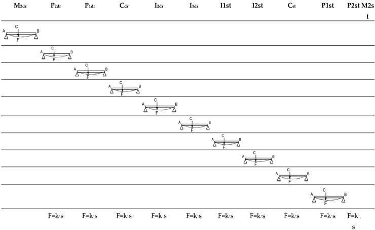 |
Table 3.
The distances L, a, and s measured along the curve of the orthodontic archwire.
| M1dr | Cdr | I2dr | I1dr | I1st | I2st | Cst | M1st | M2st | |
| L [mm] | 29.75 | 16.23 | 23.17 | 22.34 | 16.61 | 31.8 | 34.93 | ||
| a [mm] | 22.94 | 7.36 | 8.87 | 14.3 | 8.04 | 8.57 | 23.23 | 11.7 | |
| s [mm] | 1.41 | 2.31 | 2.09 | 2.22 | 1.88 | 1.65 | 2.29 |
Table 4.
The distances L, a, and s measured along the curve of the orthodontic archwire—mandible.
| M2dr | P2dr | P1dr | Cdr | I2dr | I1dr | I1st | I2st | Cst | P1st | P2st | M2st | |
| L [mm] | 29.8 | 16.21 | 16.45 | 15.21 | 15.1 | 14.02 | 14.53 | 16.34 | 16.9 | 28.38 | ||
| a [mm] | 22.96 | 6.93 | 9.28 | 7.17 | 8.04 | 7.1 | 6.92 | 7.61 | 8.73 | 8.17 | 20.21 | |
| s [mm] | 1.41 | 0.6 | 1.41 | 1.54 | 1.21 | 1.01 | 1.31 | 1.05 | 0.97 | 1.5 |
Table 5.
Values of the forces F and the reactions V exerted on the maxillary orthodontic archwire.
| M1dr | Cdr | I2dr | I1dr | I1st | I2st | Cst | M1st | M2st | |
| F [N] | 0.0612 | 0.3833 | 0.12681 | 0.15626 | 0.28816 | 0.04856 | 0.04419 | ||
| V [N] | 0.04725 | 0.1738 | 0.0625 | 0.30955 | 0.21775 | 0.06932 | 0.17807 | 0.02938 | 0.014 |
Table 6.
Values of the forces F and the reactions V developed along the curve of the orthodontic archwire in the mandible.
Table 6.
Values of the forces F and the reactions V developed along the curve of the orthodontic archwire in the mandible.
| M2dr | P2dr | P1dr | Cdr | I2dr | I1dr | I1st | I2st | Cst | P1st | P2st | M2st | |
| F [N] | 0.0596 | 0.1016 | 0.2272 | 0.3083 | 0.24 | 0.2571 | 0.3004 | 0.1698 | 0.14 | 0.05 | ||
| V [N] | 0.04 | 0.0434 | 0.1420 | 0.2035 | 0.2295 | 0.29 | 0.2583 | 0.2700 | 0.3147 | 0.18 | 0.06 | 0.04 |
Disclaimer/Publisher’s Note: The statements, opinions and data contained in all publications are solely those of the individual author(s) and contributor(s) and not of MDPI and/or the editor(s). MDPI and/or the editor(s) disclaim responsibility for any injury to people or property resulting from any ideas, methods, instructions or products referred to in the content. |
© 2026 by the authors. Licensee MDPI, Basel, Switzerland. This article is an open access article distributed under the terms and conditions of the Creative Commons Attribution (CC BY) license (http://creativecommons.org/licenses/by/4.0/).
Copyright: This open access article is published under a Creative Commons CC BY 4.0 license, which permit the free download, distribution, and reuse, provided that the author and preprint are cited in any reuse.