

Submitted:
17 August 2026
Posted:
17 August 2026
You are already at the latest version
Abstract
Environmental taxation is an important instrument in the transition to a low-carbon economy, yet empirical findings on its relationship with economic growth remain inconclusive. This study examines whether public debt moderates the relationship between environmental tax revenue and real GDP growth in the EU-27. It uses a balanced panel of 297 observations covering 2014–2024. The baseline specification is a two-way fixed-effects model with Driscoll–Kraay standard errors, supplemented by marginal-effects analysis and robustness checks. At the mean level of the other interacting variable, neither environmental tax revenue nor public debt exhibits a statistically significant conditional association with economic growth. However, the interaction coefficient is negative and statistically significant, indicating that the estimated relationship between environmental tax revenue and growth becomes less favourable as public debt increases. The marginal effect is positive and statistically significant at low debt levels, statistically insignificant at the mean debt level, and negative but statistically insignificant at high debt levels. Robustness checks preserve the negative sign of the interaction, although its statistical significance depends on the covariance estimator used. The findings indicate that fiscal conditions matter for the environmental taxation–growth relationship, but they do not establish a causal effect or a universal debt threshold.
Keywords:
environmental taxation
; economic growth
; public debt
; moderating effect
; fiscal sustainability
; panel data
; European Union
1. Introduction
The transition to a low-carbon and resource-efficient economy has made environmental taxation a key instrument in contemporary tax policy for addressing activities that adversely affect the environment. Its primary purpose is to internalise externalities by correcting and compensating for environmental costs that are not reflected in market prices. Alongside this environmental function, environmental taxes generate public revenue that may be used to finance green investment, technological upgrading, social compensation, or reductions in other, more distortionary taxes. This feature, associated with the so-called double dividend (Metcalf, 2003), distinguishes environmental taxes from other forms of taxation.
The relationship between environmental taxation and economic growth is nevertheless not unambiguous. In the short term, a higher tax burden on environmentally harmful activities may raise firms’ costs, constrain investment, and weaken the price competitiveness of energy-intensive industries. Over a longer horizon, however, the same taxes may stimulate technological innovation and energy efficiency, alter the structure of production, and redirect resources towards more productive and environmentally sustainable activities. The eventual outcome also depends on how the revenue is used, the country’s institutional quality and economic structure, and the broader fiscal environment.
Public debt occupies a particularly important position in this context. Its level reflects not only the accumulated fiscal burden but also the government’s capacity to finance investment, implement compensatory policies, and respond to economic shocks. Countries with lower debt generally have greater fiscal space to direct environmental tax revenue towards green infrastructure, energy efficiency, and technological upgrading. At high levels of public debt, by contrast, budgetary resources may be constrained by debt-servicing costs and the need for fiscal consolidation.
The existing literature reports mixed findings on the relationship between environmental taxation and economic growth (Fullerton & Metcalf, 1997; Porter & van der Linde, 1995). Some studies identify positive associations related to innovation (Bovenberg & Goulder, 2001), resource efficiency, and the recycling of tax revenue. Others report negative or statistically insignificant relationships attributable to higher production costs, reduced competitiveness, and cross-country differences in tax and institutional systems. These divergent findings suggest that examining only an average relationship between environmental taxes and economic growth may be insufficient. It is also necessary to identify the conditions under which environmental taxation is associated with stronger or weaker economic performance (de Bruin et al., 2019; Gueret et al., 2024).
This study contributes to this debate by treating public debt not merely as an independent macroeconomic factor but as a moderator of the relationship between environmental tax revenue and economic growth. Its central research question is whether the estimated relationship between environmental taxation and growth varies with the level of public debt across EU Member States. This approach moves beyond the search for a single universal effect and instead evaluates a conditional relationship in which the same tax instruments may be associated with different outcomes under different levels of public indebtedness.
Accordingly, the study aims to evaluate the conditional relationship among environmental tax revenue, public debt, and economic growth, and to determine whether this relationship varies with the level of public debt. The analysis uses balanced panel data from Eurostat for the 27 EU Member States over the period 2014–2024. The empirical strategy comprises pooled ordinary least squares (Pooled OLS), fixed-effects and random-effects models, and a two-way fixed-effects specification. The preferred specification controls for both time-invariant unobserved country characteristics and common time shocks. Because the diagnostic tests indicate dependence in the residuals, statistical inference is based on Driscoll–Kraay standard errors. Marginal effects of environmental tax revenue are also estimated at different levels of public debt to provide a substantively meaningful interpretation of the moderating relationship.
The remainder of the article is organised as follows. The next section presents the theoretical framework, reviews the relevant literature, identifies the research gap, and develops the hypotheses. Section 3 describes the data, variables, and econometric methodology. Section 4 reports the descriptive statistics, correlation analysis, diagnostic tests, model-selection results, baseline estimates, marginal effects, and robustness checks. Section 5 discusses the findings, while the final section presents the main conclusions, policy implications, limitations, and directions for future research.
2. Literature Review and Hypothesis Development
2.1. Theoretical Framework
In recent years, environmental taxes have become a key market-based instrument for promoting sustainable development and supporting the transition to a low-carbon economy. This is partly because they differ from other forms of taxation through the so-called double dividend they may generate. Unlike traditional fiscal instruments, environmental taxes pursue two objectives. First, they seek to internalise the external costs associated with environmental degradation. At the same time, they generate public revenue that can subsequently be used to finance green investment, reduce other distortionary taxes, or support fiscal consolidation. The theoretical foundations of environmental taxation derive from the Pigouvian taxation concept (Pigou, 1920), according to which taxes imposed on environmentally harmful activities correct market failures by incorporating the social costs of pollution into market prices. This approach can improve allocative efficiency by encouraging producers and consumers to reduce environmentally harmful behaviour and adopt cleaner technologies (Goulder, 1994; Bovenberg & de Mooij, 1994).
Alongside the development of the double-dividend theory, research has also examined the potentially divergent economic consequences of environmental taxes. The relevant studies and their findings can broadly be divided into two groups. The first group suggests that environmental taxation may be positively associated with economic growth. According to the Porter hypothesis, appropriately designed environmental standards can encourage firms to use resources more efficiently (Porter, 1991). This may reduce waste and energy intensity, improve production processes, and stimulate the development of new products. Consequently, part of the cost of regulatory compliance may be offset by so-called innovation offsets arising in response to regulatory pressure (Porter & van der Linde, 1995). Based on 139 simulations reported in 56 studies evaluating the effects of environmental tax reform on CO₂ emissions, employment, economic activity, investment, and consumer prices, Bosquet (2000) concludes that environmental taxes produce positive or neutral outcomes in a substantial proportion of the studies examined. Such outcomes are particularly likely when the revenue is used effectively, for example, to reduce other highly distortionary taxes or support employment. Bosquet does not, however, argue that environmental taxes automatically generate economic growth. Rather, the outcomes are conditional on the design of the reform, the use of the revenue generated, labour-market characteristics, and the broader macroeconomic environment (Andersen, 2010; Metcalf & Stock, 2023).
Similar findings are reported in other empirical studies (Gurtu et al., 2022; He et al., 2019; Mirović et al., 2021; Radulescu et al., 2017). These studies support the proposition that environmental taxation may improve energy efficiency, stimulate technological innovation, and enhance productivity, particularly when environmental tax revenue is used to reduce taxes on labour or corporate activity or is redirected towards green public investment.
The second group of studies suggests that environmental taxation may increase production costs, reduce firms’ international competitiveness, and discourage investment, particularly in energy-intensive industries. Such adverse effects may arise when environmental tax revenue is used primarily to improve fiscal balances rather than to finance productive investment or compensate affected households and firms (Bovenberg and Goulder 2001; Freire-González 2018; Fullerton and Metcalf 1997).
More recent empirical research increasingly indicates that the economic consequences of environmental taxation are highly context-dependent and are influenced by how the revenue generated is used (Saramas et al., 2026). Environmental taxes do not produce identical outcomes across countries. Their effectiveness depends on institutional quality, economic structure, the design of environmental tax reforms, revenue-recycling mechanisms, and broader fiscal conditions. Existing studies indicate that differences in national fiscal capacity and policy implementation contribute substantially to the heterogeneous macroeconomic outcomes observed across countries (de Bruin et al., 2019; Guéret et al., 2024; Halidu et al., 2025).
A growing body of research links environmental taxation to fiscal sustainability and public debt. Fodha et al. (2018) examine environmental policies financed through taxation or public borrowing and argue that reducing public debt may support both capital accumulation and environmental quality.
Using a dynamic game-theoretic framework, Halkos and Papageorgiou (2018) establish a direct theoretical link between pollution, environmental taxation, and public debt. Their analysis highlights the strategic tension faced by governments that must simultaneously reduce pollution and maintain debt sustainability. Similarly, Rausch (2013) examines the use of carbon tax revenue to consolidate public debt and shows that such a policy may generate long-term welfare gains by reducing future interest obligations. Davin et al. (2025) theoretically investigate whether an economy can simultaneously sustain economic growth, finance anti-pollution measures through public debt, and avoid unsustainable debt and environmental dynamics. Their central argument is that public debt does not necessarily constitute only a constraint on economic growth. When debt is used to finance effective pollution-control measures and adaptation to environmental damage, it may indirectly support productivity and growth.
2.2. Scientific Gap and Hypothesis Development
Most of the existing literature examines the relationship between environmental taxation and economic growth separately from the relationship between environmental policy and fiscal sustainability. Empirical studies integrating environmental tax revenue, public debt, and economic growth within a unified analytical framework remain limited. More specifically, public debt is generally treated as an independent determinant of growth, an indicator of fiscal sustainability, or an outcome of fiscal policy. It is rarely examined as a factor that may alter the strength and direction of the relationship between environmental taxation and economic growth. Consequently, it remains insufficiently understood whether the same environmental tax policy is associated with different growth outcomes at low and high levels of public indebtedness.
This study addresses this gap by treating public debt not only as an independent explanatory variable but also as a moderator of the relationship between environmental tax revenue and economic growth. The analysis, therefore, moves beyond estimating a universal average effect and examines the conditions under which environmental taxation may be associated with stronger or weaker economic performance. In this way, the study empirically integrates three strands of research that have largely been examined separately: environmental taxation, fiscal sustainability, and economic growth. These dimensions are incorporated into a common panel-data framework for the EU Member States, together with a set of relevant control variables.
Based on the theoretical framework, the identified research gap, and the findings of previous empirical studies, three research hypotheses are formulated. Because the econometric model includes an interaction term between environmental tax revenue and public debt, the estimated relationship of each variable with economic growth is conditional on the level of the other variable. To facilitate the interpretation of the main coefficients, environmental tax revenue and public debt are mean-centred. Accordingly, coefficient (\beta_1) represents the conditional association between environmental tax revenue and economic growth at the sample mean level of public debt, whereas (\beta_2) represents the conditional association between public debt and economic growth at the sample mean level of environmental tax revenue.
Hypothesis 1 (H₁):
At the sample mean level of public debt, environmental tax revenue is positively associated with economic growth in the EU Member States:
H1: β1 > 0
where β1 is the coefficient on the environmental tax revenue variable and represents its conditional association with economic growth when the mean-centred value of public debt equals zero.
The expected positive sign is based on the capacity of environmental taxation to promote resource and energy efficiency, stimulate technological innovation, and support the productive use of the revenue generated.
Hypothesis 2 (H2):
At the sample mean level of environmental tax revenue, public debt is negatively associated with economic growth in the EU Member States:
H2: β2 < 0
where β2 is the coefficient on the public debt variable and represents its conditional association with economic growth when the mean-centred value of environmental tax revenue equals zero.
The expected negative sign is based on the proposition that higher public debt may increase debt-servicing costs, constrain fiscal space, and reduce governments’ capacity to undertake productive public investment.
Hypothesis 3 (H3):
Public debt negatively moderates the relationship between environmental tax revenue and economic growth, such that the marginal effect of environmental tax revenue decreases as public debt increases:
H3: β3 < 0
where β3 is the coefficient on the interaction term between the mean-centred values of environmental tax revenue and public debt, a negative coefficient indicates that, as public debt increases, the estimated relationship between environmental tax revenue and economic growth becomes less favourable. This hypothesis represents the central proposition of the study because it tests whether the relationship between environmental taxation and growth varies with a country’s fiscal position.
3. Materials and Methods
3.1. Research Design
This study employs a quantitative research design using balanced panel data to examine the relationship between environmental tax revenue and economic growth in EU Member States, with particular emphasis on the moderating role of public debt. Panel-data analysis is especially appropriate for this type of research because it combines the cross-sectional and time dimensions of the data. It therefore permits the analysis of both within-country changes over time and cross-country differences (Baltagi, 2005; Hsiao, 2014; Wooldridge, 2010). Compared with purely cross-sectional or time-series approaches, panel models provide more observations, may improve estimation efficiency, and reduce the risk of bias from unobserved time-invariant country characteristics.
The empirical analysis is based on a balanced panel comprising the EU-27 countries over the period 2014–2024, yielding a total of 297 observations. The selected period covers several major economic and policy developments, including the implementation of the European Green Deal, the COVID-19 pandemic, the subsequent energy crisis, and the inflationary shock. It therefore provides an appropriate setting for examining whether the estimated relationship between environmental tax revenue and economic growth remains consistent across different macroeconomic conditions.
The empirical analysis follows a sequential research strategy. First, descriptive statistics and correlation analysis are used to examine the main characteristics of the variables and their preliminary relationships. Multicollinearity is then assessed using variance inflation factors (VIFs), which indicate whether the explanatory variables can be included simultaneously in the regression model without substantial problems arising from linear dependence among them (O’Brien, 2007).
The econometric analysis subsequently proceeds from simpler to more complex panel-data specifications. Pooled ordinary least squares (Pooled OLS) is estimated as the baseline model, followed by fixed-effects and random-effects models that account for unobserved country heterogeneity. The selection of the most appropriate specification is based on standard panel-data tests, including the F-test for individual effects, the Breusch–Pagan Lagrange multiplier test (Breusch & Pagan, 1980), and the Hausman test (Hausman, 1978).
Given the presence of common economic shocks affecting all countries during the period examined, the preferred specification is a two-way fixed-effects model that simultaneously controls for country-specific characteristics and common time effects. Following model selection, diagnostic tests are conducted for heteroskedasticity, serial correlation, and cross-sectional dependence among the panel units (Breusch & Pagan, 1979; Drukker, 2003; Wooldridge, 2010). The detected violations of the classical assumptions motivate the use of Driscoll–Kraay standard errors (Driscoll & Kraay, 1998), which provide inference robust to heteroskedasticity, serial correlation, and cross-sectional dependence.
In the final stage of the analysis, the marginal effects of environmental tax revenue are estimated at different levels of public debt to facilitate an accurate interpretation of the moderating relationship. The robustness of the results is also examined using alternative covariance estimators and different lag specifications for the standard errors.
The methodological framework is designed to progress systematically from identifying simple statistical relationships to estimating conditional associations. This makes it possible to examine not only whether environmental tax revenue is associated with economic growth, but also how this association changes under different fiscal conditions. The overall methodological framework, research strategy, and analytical sequence are presented in Figure 1.
3.2. Data and Variables
The main characteristics of the variables used in the study are summarised in Table 1.
The dependent variable is the annual real GDP growth rate at market prices, measured as the percentage change in chain-linked volumes relative to the previous year. This measure captures changes in the real volume of economic activity, excluding the effects of inflation, and is widely used as an indicator of economic growth in cross-country analyses.
Environmental tax revenue is selected as the main explanatory variable because environmental taxes are an important market-based instrument whose principal purpose is to internalise the negative externalities generated by environmentally harmful activities. By increasing the cost of pollution, environmental taxes may alter the behaviour of economic agents, encouraging them to adopt cleaner technologies and improve resource efficiency. At the same time, they generate public revenue that can finance investments in support of the green transition. This combination of environmental and fiscal functions underlies the concept of the double dividend.
The environmental taxation indicator used in the analysis is total environmental tax revenue as a percentage of GDP. It measures the relative fiscal significance, or revenue intensity, of environmental taxation in the national economy and facilitates comparisons among countries of different economic sizes. However, the indicator should not be interpreted directly as a measure of tax rates or of the stringency or effectiveness of environmental policy. Tax rates, the size and composition of the taxable base, the behaviour of economic agents, and GDP dynamics jointly determine its value.
Expressing environmental tax revenue as a percentage of GDP captures its significance relative to the economy as a whole rather than as a nominal amount. This reduces the influence of differences in the size of European economies and facilitates comparisons among countries with different economic structures and levels of development. The indicator reflects the importance of environmental taxation in each national economy’s revenue. It also ensures methodological consistency with other variables in the model, such as public debt and investment, which are likewise expressed relative to GDP.
Unlike the other variables, the expected sign of environmental tax revenue is theoretically ambiguous and may be either positive or negative. This ambiguity is partly related to the time horizon over which the relationship is evaluated. In the short term, environmental taxes may be associated with weaker economic growth due to higher production costs and energy prices, reduced investment, and constrained consumption. Over the longer term, however, they may stimulate innovation, resource and energy efficiency, and green investment (Blagoeva & Georgieva, 2023; Krastev & Krasteva-Hristova, 2024). They also generate revenue that may be used to reduce other taxes or finance green investment, thereby potentially supporting economic growth (Blagoeva & Georgieva, 2021).
Previous empirical studies likewise report mixed findings concerning the sign of this relationship. Some identify a negative association attributable to higher production costs and reduced competitiveness (Hassan et al., 2020). Others report a strong positive association operating through improvements in energy efficiency and innovation (Kalaš et al., 2025). Abdullah and Morley (2014) find evidence of causality between environmental taxation and economic growth, but do not confirm a clear growth-enhancing effect.
The next variable included in the model is public debt. Public debt is a key indicator of fiscal sustainability and a government’s financial capacity. Its level may be associated with economic growth through several channels. High public indebtedness increases debt-servicing costs, constrains the fiscal space available for productive public investment, raises sovereign risk, and may discourage private investment by increasing uncertainty and expectations of future taxation. Excessive public debt may therefore constrain long-term economic growth, particularly in highly indebted economies. Accordingly, its expected coefficient is negative.
In addition to its inclusion as an explanatory variable, public debt is specified as a moderating variable. The underlying argument is that public debt may not only be directly associated with economic growth but also alter the relationship between environmental tax revenue and growth. Countries with low public indebtedness generally have greater fiscal capacity to invest and to support firms and households. Under these conditions, environmental tax revenue may be channelled towards green investment, innovation, and productivity improvements. The opposite may apply in highly indebted countries, where substantial debt-servicing costs and budgetary constraints reduce the resources available for green programmes, technological modernisation, compensation for households and firms, or reductions in other taxes. Consequently, the relationship between environmental taxation and growth may become less favourable and may potentially turn negative. The estimated association, therefore, depends on the fiscal environment in which environmental taxation is implemented.
This reasoning motivates the moderating role assigned to public debt: rather than merely being associated with economic growth, debt may modify the relationship between environmental tax revenue and growth. To capture this moderating relationship, an interaction term between environmental tax revenue and public debt is introduced into the regression model (Aiken & West, 1991). The interaction coefficient is expected to be negative because higher public debt may weaken the potentially favourable association between environmental taxation and economic growth by limiting governments’ fiscal capacity to direct revenue towards productive investment or other compensatory measures.
Gross fixed capital formation is included as a measure of investment activity in the economy. It captures acquisitions of fixed assets, including machinery, equipment, infrastructure, buildings, and intellectual property products, that expand the economy’s productive capacity. Because investment is one of the principal drivers of long-term economic growth, gross fixed capital formation is widely used in empirical growth models. In the present study, the indicator is expressed as a percentage of GDP. This measures the relative importance of investment activity within the national economy while ensuring comparability among countries at different levels of economic development.
Gross fixed capital formation is also included as a control variable to account for investment activity when estimating the conditional relationship between environmental tax revenue and economic growth. Inflation and unemployment are included as additional controls. Collectively, these variables account for other macroeconomic factors related to economic growth, thereby reducing the risk of omitted-variable bias and improving the precision of the estimated conditional association between the main explanatory variable and the outcome.
Inflation is measured using the Harmonised Index of Consumer Prices (HICP). The HICP is the standard measure used within the EU framework and is compiled according to a common methodology across all EU Member States, ensuring a high degree of comparability. This characteristic is particularly important in multi-country panel-data analysis, where methodological consistency is essential for obtaining comparable estimates. The selected unit of measurement is the annual average rate of change because it reflects the general inflationary environment over the year rather than short-term price fluctuations. Annual averages reduce the influence of temporary shocks and seasonal variation, making the indicator more appropriate for panel analyses based on annual macroeconomic data. Moreover, the annual inflation rate matches the frequency of the other variables included in the model, ensuring consistency across the dataset.
Inflation is included as a control variable because macroeconomic price stability is an important factor associated with economic growth. Inflation affects the purchasing power of households and firms, their investment decisions, and overall macroeconomic stability. Environmental taxation may also be indirectly associated with inflation through higher prices for energy and other environmentally intensive goods and services. Controlling for inflation, therefore, allows the model to distinguish the conditional relationship between environmental tax revenue and economic growth from relationships transmitted through changes in the general price level.
The expected coefficient on inflation is negative because high inflation is associated with declining purchasing power, greater economic-policy uncertainty, and weaker incentives to invest. However, the nature of this relationship also depends on the inflation rate itself. Low and stable inflation is often regarded as compatible with, and potentially supportive of, economic growth.
The final variable included in the model is unemployment among the economically active population aged 15–74. The indicator is measured in accordance with the International Labour Organisation (ILO, 2013) definition and harmonised by Eurostat through the EU Labour Force Survey (Eurostat, 2024), ensuring methodological consistency and comparability across EU Member States. The unemployment rate reflects the degree of labour-market utilisation and is a key indicator of macroeconomic stability and growth. It is measured as the percentage of the labour force aged 15–74 that is willing and able to work but unable to find employment. Measuring unemployment relative to the labour force rather than the total population provides a more accurate indication of labour-market conditions and facilitates meaningful comparisons among countries with different demographic structures. It also excludes the influence of economically inactive groups, such as pensioners and students.
Unemployment is included as a control variable because labour-market conditions are closely related to economic growth. High unemployment indicates underutilisation of labour resources, which is associated with lower household income, weaker aggregate demand, and reduced economic activity. Environmental taxes may also be associated with labour-market outcomes through their implications for firms’ production costs, employment decisions, and sectoral restructuring. Including unemployment as a control variable, therefore, helps distinguish the conditional relationship between environmental tax revenue and economic growth from the relationships operating through labour-market conditions.
The expected coefficient on unemployment is negative because higher unemployment implies weaker utilisation of labour resources, lower household consumption, reduced investment incentives, and lower aggregate demand, all of which are associated with slower economic growth.
Environmental taxes may increase production costs, particularly in carbon-intensive industries, and may therefore be associated with short-term employment adjustments. At the same time, they may stimulate job creation in environmentally sustainable sectors through green investment and technological innovation. Labour-market conditions thus represent an important transmission channel through which environmental taxation may be indirectly related to economic growth.
3.3. Baseline Empirical Specification
The empirical analysis is based on a balanced panel dataset covering the EU-27 Member States over the period 2014–2024. The dependent variable is real GDP growth, while environmental tax revenue is the main explanatory variable. Public debt is included both as an explanatory variable and as a moderator of the relationship between environmental tax revenue and economic growth. To facilitate interpretation of the interaction term and reduce nonessential multicollinearity, environmental tax revenue and public debt are mean-centred before constructing the interaction term.
The baseline empirical specification is defined as follows:
where: i=1,...,27 denotes the country;
GDPGrowthit = β0 + β1EnvTaxesc,it + β2Debtc,it + β3(EnvTaxesc,it х Debtc,it)+β4Investit + β5Inflit +β6UnEmplit + εit
t = 2014,..., 2024 denotes the year;
β0 - interceipt;
β1, β2, β3, β4, β5, β6 the regression coefficients;
EnvTaxesc, it , Debtc,it , EnvTaxesc,it х Debtc,it is the mean-centred value of environmental tax revenue for country (i) in year (t);
Debt c,it is the mean-centred value of public debt for country (i) in year (t);
EnvTaxesc, it x Debtc, it is the interaction term between the two mean-centred variables;
Investit, Inflit, UnEmplit are the control variables for investment, inflation, and unemployment, respectively; and
εit – idiosyncratic error.
4. Results
4.1. Descriptive Statistics
Descriptive statistics summarise the main characteristics of the variables and provide information on their variation, skewness, and potential extreme observations. The results for the balanced panel of 297 observations are presented in Table 2.
The average annual real GDP growth rate is 2.62%. with a standard deviation of 3.72 percentage points and a range from −10.90% to 24.60%. The wide range and positive excess kurtosis reflect the influence of exceptional macroeconomic events during the period examined. Environmental tax revenue averages 2.60% of GDP and exhibits limited variation. ranging from 0.85% to 5.62% of GDP.
The greatest heterogeneity is observed in public debt, which averages 68.81% of GDP and ranges from 8.50% to 209.40% of GDP. Its positive skewness reflects the presence of a limited number of highly indebted countries. This substantial variation provides an appropriate empirical basis for examining the moderating role of public debt in the relationship between environmental tax revenue and economic growth.
The mean value of gross fixed capital formation is 21.44% of GDP. The high skewness and excess kurtosis of investment are primarily attributable to extreme observations, most notably that for Ireland in 2019. Inflation and unemployment also exhibit positive skewness and substantial variation. Inflation mainly reflects the price and energy shocks of 2022–2023, whereas differences in unemployment reflect the heterogeneous conditions prevailing in national labour markets.
Overall, the variables exhibit considerable heterogeneity both across countries and over time. Environmental tax revenue has a comparatively more stable distribution, whereas public debt, investment, inflation and unemployment display more pronounced extreme values. These characteristics should be considered when interpreting the subsequent panel estimates and robustness checks.
4.2. Correlation Analysis
Descriptive statistics alone do not provide information on the direction and strength of the relationships among the selected variables. Therefore, the next stage of the analysis employs Pearson correlation coefficients (Rodgers & Nicewander, 1988). The correlation analysis evaluates the direction and strength of the linear relationships among the variables and provides a preliminary assessment of potential multicollinearity before the panel model is estimated. The results are presented in Table 3.
As shown in the table, the Pearson correlation coefficients indicate relatively weak to moderate linear relationships among the explanatory variables. The strongest correlation is observed between public debt and unemployment (r = 0.614). followed by a negative correlation between gross fixed capital formation and unemployment (r = - 0.425). None of the pairwise correlation coefficients exceeds the commonly used diagnostic threshold of 0.70. These results suggest that severe multicollinearity is unlikely to affect the regression estimates materially. Nevertheless, multicollinearity is examined further using variance inflation factors (VIFs) in the subsequent analysis.
The correlations between GDP growth and the explanatory variables are generally weak. However, weak bivariate correlations do not imply the absence of a relationship among the variables. Rather, they suggest that the relationships may be more complex, may depend on other macroeconomic factors, and may vary across different levels of public debt. Consequently, the relationship between economic growth and the selected indicators is unlikely to be adequately captured by simple bivariate associations. A multivariate panel regression model is therefore appropriate because it permits the simultaneous estimation of the conditional associations of environmental tax revenue, public debt, their interaction, and the selected control variables, while controlling for unobserved country-specific heterogeneity.
Although Pearson correlation coefficients provide preliminary information on the direction and strength of linear relationships among variables, they are insufficient for assessing multicollinearity in a multivariate regression model. An additional diagnostic assessment is therefore performed using the variance inflation factor (VIF) and tolerance statistics. Because the final model specification includes an interaction term between environmental tax revenue and public debt, the two variables are mean-centred before constructing the interaction term. Mean-centring is widely recommended in moderation models because it facilitates the interpretation of the main coefficients and may reduce nonessential multicollinearity between the interaction term and its constituent variables (Aiken & West, 1991; Shieh, 2011). The results are presented in Table 4.
As shown in Table 4, the VIF values range from 1.158 to 1.932. whereas the tolerance values range from 0.518 to 0.863. All VIF values are well below both the conservative threshold of 3 and the commonly used threshold of 5. At the same time, all tolerance values exceed the recommended minimum of 0.20. These results indicate that the explanatory variables do not exhibit problematic multicollinearity and that the inclusion of the interaction term does not create substantial collinearity with its constituent variables. The selected variables can therefore be retained in the subsequent panel regression analysis.
4.3. Panel Model Specifications
To determine the most appropriate empirical specification, four alternative panel models are estimated and compared: pooled OLS, one-way fixed effects, random effects and two-way fixed effects. These models differ primarily in their treatment of unobserved country-specific heterogeneity and common time-specific shocks.
The pooled OLS model is used as the baseline specification. combining all country-year observations into a single regression. It does not control for unobserved country-specific characteristics and assumes that the intercept β0 is identical across all countries in the sample. The intercept represents the expected value of economic growth when all explanatory variables equal zero. Because pooled OLS disregards cross-country heterogeneity, its estimates are used primarily as a benchmark for comparison with panel estimators that account for country-specific characteristics.
The analysis. therefore. proceeds with the one-way fixed-effects model. specified as follows:
where:
GDPGrowthit = αi + β1EnvTaxesc.it + β2Debtc.it + β3(EnvTaxesc.it х Debtc.it)+β4Investit + β5Inflit +β6UnEmplit + εit
αi - denotes the country fixed effect
αi=β0+ui - represents the country-specific component.
The one-way fixed-effects model controls for unobserved time-invariant heterogeneity across countries.
The random-effects model also accounts for country-specific heterogeneity but treats it as a random component:
GDPGrowthit = β0 + β1EnvTaxesc.it + β2Debtc.it + β3(EnvTaxesc.it х Debtc.it)+β4Investit + β5Inflit +β6UnEmplit + ui + εit
The key assumption underlying the random-effects estimator is that the unobserved country-specific effect is uncorrelated with the explanatory variables:
Cov(ui,Xit)=0
If this assumption holds, the random-effects estimator is more efficient than the fixed-effects estimator. If the assumption is violated, however, the random-effects estimates may be inconsistent.
Finally, the two-way fixed-effects model extends the one-way specification by including both country and year effects:
where λt denotes year fixed effects.
GDPGrowthit = αi + λt + β1EnvTaxesc.it + β2Debtc.it + β3(EnvTaxesc.it х Debtc.it)+β4Investit + β5Inflit +β6UnEmplit + εit
Country fixed effects control for unobserved time-invariant differences among the EU Member States, whereas year fixed effects capture common shocks affecting all countries in a given year. This is particularly important for the 2014–2024 period, which includes major common shocks such as the COVID-19 pandemic, the energy crisis, inflationary pressures, and coordinated policy responses.
Driscoll–Kraay standard errors do not change the model specification or the estimated coefficients. Instead, they adjust the standard errors, (t)-statistics and (p)-values to provide inference that is robust to heteroskedasticity, serial correlation, and cross-sectional dependence.
After the alternative panel specifications are estimated, formal model-selection tests are applied. First, the F-test for individual effects is used to compare the pooled OLS with the fixed-effects model. Second, the Breusch–Pagan Lagrange multiplier test is used to compare pooled OLS with the random-effects model. Third, the Hausman test is used to distinguish between the fixed-effects and random-effects estimators.
F-Test: Pooled OLS versus Fixed Effects
An F-test for individual effects is conducted to determine whether the fixed-effects model provides a more appropriate representation of the data than the pooled OLS model. The null hypothesis assumes the absence of country-specific individual effects; at the same time, the alternative hypothesis allows for country-specific characteristics. Rejection of the null hypothesis indicates that pooled OLS is inappropriate and that a fixed-effects specification should be preferred.
H0 : αi = α for all countries
H1 : αi ≠ α for at least some countries
The test results (F=2.930). (p<0.001) lead to rejection of the null hypothesis. This indicates the presence of statistically significant country-specific effects and shows that a pooled OLS specification is not appropriate.
Breusch–Pagan LM Test: Pooled OLS versus Random Effects
The Breusch–Pagan Lagrange multiplier test evaluates whether random effects are present. Rejection of the null hypothesis indicates that a random-effects specification is preferable to a pooled OLS specification.
H0 : Var( ui ) = 0.
Under the null hypothesis, there are no statistically significant cross-country differences in the unobserved effects, and pooled OLS may therefore be sufficient.
H1 : Var( ui ) > 0 .
Under the alternative hypothesis, statistically significant differences exist across countries. implying that pooled OLS is inappropriate and that a panel-data model, such as fixed-effects or random-effects, should be used.
The Breusch–Pagan LM test results (χ² = 14.425; p < 0.001) lead to rejection of the null hypothesis. The results, therefore, confirm the presence of statistically significant panel effects and indicate that pooled OLS is not appropriate.
Hausman Test: Fixed Effects versus Random Effects
H0 : Cov (ui, Xit) = 0.
H1 : Cov (ui, Xit) ≠ 0
H1 : Cov (ui, Xit) ≠ 0
The Hausman test examines whether the unobserved country-specific effects are correlated with the explanatory variables:
The null hypothesis implies that the random-effects estimator is consistent and efficient; at the same time, the alternative hypothesis indicates that the fixed-effects estimator is more appropriate. The test results (χ² = 12.192; p = 0.058) do not permit rejection of the null hypothesis at the conventional 5% significance level. However, the null hypothesis is rejected at the 10% level, providing marginal evidence in favour of the fixed-effects estimator. Given the theoretical likelihood that unobserved country-specific characteristics are correlated with fiscal and macroeconomic variables, the fixed-effects framework remains the methodologically preferred specification.
4.4. Diagnostic Tests
In addition to the model-selection tests, a series of diagnostic tests is conducted to assess whether statistical inference from the selected panel model can be interpreted reliably. Whereas the model-selection tests determine whether pooled OLS, fixed effects, or random effects provide the more appropriate specification, the diagnostic tests evaluate whether the assumptions concerning the structure of the error term are satisfied.
This assessment is important because it addresses violations such as heteroskedasticity, serial correlation, and cross-sectional dependence, which can render conventional standard errors unreliable and lead to misleading conclusions about statistical significance, even when the estimated coefficients remain unchanged. The diagnostic analysis. therefore. examines three potential problems:
First, the Breusch–Pagan test is used to assess heteroskedasticity. The test result (BP = 11.027, p = 0.0876 > 0.05) does not permit rejection of the null hypothesis of homoskedasticity, which holds that the residuals have constant variance. Therefore, the test provides no statistically significant evidence of heteroskedasticity (see Table 5).
Second, the Breusch–Godfrey/Wooldridge and Wooldridge fixed-effects tests are applied to detect serial correlation within countries over time and in the idiosyncratic errors of the fixed-effects and random-effects specifications. The null hypothesis of no serial correlation is strongly rejected for both the fixed-effects model (χ² = 124.35, p < 0.0001) and the random-effects model (χ² = 108.83, p < 0.0001). This finding is further confirmed by the Wooldridge fixed-effects test (F = 7.011, p = 0.0086). These results indicate that conventional standard errors may be unreliable. thereby justifying the use of robust statistical inference.
Third, the Pesaran CD test is used to assess cross-sectional dependence among the EU Member States (Pesaran, 2004). The results reveal strong cross-sectional dependence in both the one-way fixed-effects model (z = 43.191, p < 0.0001) and the random-effects model (z = 44.939, p < 0.0001). These findings indicate that the residuals are correlated across countries. suggesting that the EU Member States were exposed to common shocks not captured by the one-way specifications.
To address this problem, the model is extended to include year fixed effects. Following their inclusion, the Pesaran CD test no longer rejects the null hypothesis of cross-sectional independence (z = - 0.821, p = 0.412). This suggests that the two-way fixed-effects specification adequately captures the common time-specific shocks. The evidence from the Pesaran CD tests, therefore, supports the use of a two-way fixed-effects model.
Taken together, the diagnostic tests identify serial correlation, initially strong cross-sectional dependence, and a weak indication of heteroskedasticity at the 10% significance level. These findings imply that conventional standard errors from the standard fixed-effects and random-effects models may produce unreliable statistical inference. The statistical significance of the estimated coefficients is therefore evaluated using Driscoll–Kraay standard errors, which are robust to heteroskedasticity. serial correlation. and cross-sectional dependence. The final specification thus combines two-way fixed effects with Driscoll–Kraay standard errors to control for unobserved country-specific heterogeneity and common annual shocks while providing robust inference under non-classical error dependence.
Based on the model-selection procedure and the diagnostic tests, the preferred specification is therefore the two-way fixed-effects model with Driscoll–Kraay standard errors. The main estimation results are presented in Table 6:
Table 6 presents the results from the alternative panel-data specifications. Pooled OLS is reported as the baseline specification, whereas the one-way fixed-effects and random-effects models account for unobserved country-level heterogeneity. The final column presents the preferred specification: a two-way fixed-effects model with Driscoll–Kraay standard errors. This specification controls for both time-invariant country-specific heterogeneity and common year-specific shocks, while providing inference robust to heteroskedasticity. serial correlation. and potential cross-sectional dependence.
Comparison across the models indicates that the estimated coefficients are sensitive to the treatment of unobserved heterogeneity and common time shocks. The preferred two-way fixed-effects specification controls for both country-specific unobserved heterogeneity and common annual shocks, while providing robust statistical inference.
In the preferred specification, the coefficient on environmental tax revenue is positive, however, the initial theoretical expectations allowed for either a positive or a negative sign. However. the coefficient is not statistically significant (p> 0.05, β = 0.037, p = 0.866). Because the variables entering the interaction are mean-centred, this coefficient represents the conditional association between environmental tax revenue and economic growth at the sample mean level of public debt.
The coefficient on public debt is negative. consistent with the initial expectation. but statistically insignificant (β = -0.024, p = 0.549). This coefficient represents the conditional association between public debt and economic growth at the sample mean level of environmental tax revenue.
The central finding concerns the interaction term between environmental tax revenue and public debt. Its coefficient is negative, as hypothesized, and statistically significant at the 5% level (β = - 0.020, p = 0.020). This indicates that, although public debt does not exhibit a statistically significant conditional association with GDP growth at the mean level of environmental tax revenue, it significantly moderates the relationship between environmental tax revenue and economic growth. More specifically, a one-percentage-point increase in public debt as a share of GDP reduces the estimated marginal association between a one-percentage-point increase in environmental tax revenue as a share of GDP and real GDP growth by approximately 0.020 percentage points.
The estimated relationship between environmental tax revenue and economic growth is therefore not uniform across countries but varies with their fiscal position. In lower-debt economies, environmental tax revenue may be associated with stronger economic growth, whereas this positive association weakens and may become negative as public debt increases. This result provides evidence that public debt moderates the relationship between environmental taxation and economic growth.
Among the control variables, inflation has a negative and statistically significant coefficient at the 1% level (β = - 0.134, p = 0.000000265). A one-percentage-point increase in inflation is associated with an approximately 0.134-percentage-point decrease in real GDP growth, holding the other modelled factors constant. The negative sign is consistent with the initial expectation that higher inflation may constrain economic activity by reducing purchasing power, increasing production costs and uncertainty, weakening consumption, and discouraging investment.
Unemployment also has a negative coefficient, as expected, but is only marginally significant at the 10% level (β = - 0.195, p = 0.0666). A one-percentage-point increase in unemployment is associated with an approximately 0.195-percentage-point reduction in real GDP growth, holding the other modelled factors constant. The negative sign is economically plausible because higher unemployment is associated with lower household income and consumption and with weaker utilisation of labour resources. Nevertheless, the statistical evidence for this relationship is weaker than that for inflation.
Gross fixed capital formation has a positive coefficient. consistent with the initial expectation, but it is not statistically significant in the preferred specification (β = 0.005, p = 0.956).
The preferred model has an (R2) of 0.072. indicating that the included explanatory variables account for approximately 7.2% of the within-panel variation in GDP growth after controlling for country and year fixed effects. Although the model’s explanatory power is relatively limited, this result is not unexpected given the highly volatile nature of annual real GDP growth and the influence of numerous external, cyclical, institutional and policy-related factors that are not fully captured by the specification.
More importantly, the explanatory variables are jointly statistically significant at the 1% level (F = 3.292, p = 0.0039). Thus, despite its relatively limited (R2), the model provides statistically significant evidence concerning the conditional relationship between environmental tax revenue, public debt and economic growth and is appropriate for testing the interaction between environmental taxation and public debt.
4.5. Marginal Effect of Environmental Tax Revenue at Different Levels of Public Debt
Because the interaction term between environmental tax revenue and public debt is statistically significant, the marginal effect of environmental tax revenue is estimated at different levels of public debt (Brambor et al., 2006). The results are presented in Table 7.
The values reported in Table 7 are calculated from the preferred two-way fixed-effects model with Driscoll–Kraay standard errors. The marginal effect is calculated as:
where β1 is the coefficient on environmental tax revenue
Marginal Effect = β1+β3 x Debtc.it
Marginal Effect = 0.0368268 − 0.0199784 × Debtc.it
β3 is the coefficient on the interaction term.
The marginal effects are evaluated at three levels of public debt: one standard deviation below the sample mean, at the sample mean, and one standard deviation above the sample mean. The corresponding standard errors and (p)-values are calculated using the delta method (Oehlert, 1992).
The results indicate that the marginal effect of environmental tax revenue is positive and statistically significant only at a relatively low level of public debt. At one standard deviation below the sample mean. corresponding to public debt of approximately 30.39% of GDP, the estimated marginal effect is positive and statistically significant (β = 0.804, p = 0.015). This suggests that, in economies facing fewer fiscal constraints, higher environmental tax revenue may be associated with stronger economic growth.
At the sample mean level of public debt. approximately 68.81% of GDP, the marginal effect is close to zero and statistically insignificant (β = 0.037, p = 0.866). Thus, at the sample’s average level of indebtedness, the estimated conditional association between environmental tax revenue and economic growth is not statistically distinguishable from zero.
At one standard deviation above the mean. corresponding to public debt of approximately 107.23% of GDP, the estimated marginal effect becomes negative but remains statistically insignificant (β = − 0.731, p = 0.107). The results. therefore. do not provide sufficient evidence that environmental tax revenue is associated with lower growth across highly indebted economies. They do. however. show that the positive association identified under low-debt conditions is no longer statistically supported at high debt levels. Overall, the estimated marginal association weakens and becomes non-statistically significant as public indebtedness increases. This finding provides empirical support for H₃ and suggests that the relationship between environmental taxation and economic growth is conditional on a country’s fiscal position.
The model-implied point at which the estimated marginal effect changes sign can be calculated by setting the marginal-effect expression equal to zero:
β1 + β3Debt_c = 0
0.037 − 0.020 × Debt_c = 0
0.037 − 0.020 × Debt_c = 0
Solving this expression shows that the estimated marginal effect changes sign at a mean-centred public debt value of approximately 1.84 percentage points above the sample mean Debt_c ≈ 1.84.
Given that the mean public debt in the sample is 68.81% of GDP, this corresponds to an indicative debt level of approximately 70.65% of GDP. This value should not be interpreted as a formal fiscal threshold. It is a model-implied sign-change point at which the estimated marginal association changes from positive to negative within the observed sample.
Figure 2 illustrates the conditional marginal effect of environmental tax revenue on GDP growth at different levels of public debt. The black line represents the estimated marginal effect. Its downward slope illustrates the negative moderating role of public debt. The grey area represents the 95% confidence interval calculated using Driscoll–Kraay standard errors, while the horizontal dashed line at β=0 separates positive from negative estimates.
At relatively low levels of public debt, the marginal effect is positive, indicating that environmental tax revenue may be associated with stronger GDP growth in economies facing fewer fiscal constraints. At a public debt of approximately 30% of GDP, the confidence interval does not include zero, and the estimated marginal effect is statistically significant (Debt ≈ 30%, β ≈ 0.80, p ≈ 0.015).
As public debt increases, the positive marginal effect gradually weakens and approaches zero. Around the sample mean debt level, the confidence interval includes zero, indicating that the marginal effect is no longer statistically distinguishable from zero (Debt ≈ 68%, β ≈ 0.04, p ≈ 0.866). This pattern is consistent with the negative interaction coefficient and supports H₃ in the preferred specification.
At very high levels of public debt, the estimated marginal effect becomes negative. At a debt of approximately 107% of GDP, for example, the estimate (Debt ≈ 107%, β ≈ - 0.731, p ≈ 0.107). The widening confidence interval indicates greater uncertainty at high debt levels. Consequently, although the point estimate is negative, the analysis does not provide sufficient evidence to conclude that the marginal effect is statistically negative at this debt level.
Overall, Figure 2 shows that an increase in public debt weakens the estimated favourable association between environmental tax revenue and economic growth. A positive and statistically significant conditional association is identified at relatively low levels of public debt. whereas at average and high debt levels, the estimated marginal effect is not statistically distinguishable from zero. Thus, as public indebtedness increases, the positive conditional association gradually weakens and ceases to be statistically significant.
Taken together, the results do not support statistically significant conditional associations of either environmental tax revenue or public debt with economic growth at the sample mean of the other interacting variable in the preferred two-way fixed-effects specification. However, the negative and statistically significant interaction coefficient indicates that the conditional relationship between environmental tax revenue and economic growth becomes less favourable as public debt increases. H₃ therefore receives empirical support in the preferred specification, whereas H₁ and H₂ do not.
4.6. Robustness Checks
To assess the robustness of the main empirical finding, additional specifications are estimated to examine the sensitivity of the results to the choice of standard-error estimator, the model’s time structure, and the composition of the sample. The results of these robustness checks are presented in Table 8:
For maximum temporal lags ranging from one to four years, the interaction coefficient retains its negative sign and remains statistically significant at the 5% level, with (p)-values ranging from 0.014 to 0.029. When standard errors are clustered by country, the estimated coefficient remains unchanged (β = − 0.020) but is not statistically significant (p = 0.318), indicating that the statistical inference is sensitive to the choice of covariance estimator.
In the model in which all regressors are lagged by one year, the interaction term remains negative and statistically significant when Driscoll–Kraay standard errors are used (β = −0.013; p = 0.037). Excluding 2020 and 2021 also produces an estimate close to the baseline coefficient (β = −0.020; p = 0.034). In the leave-one-country-out analysis, the interaction coefficient remains negative in all 27 specifications and is statistically significant at the 5% level in 25 of them.
Taken together, the robustness checks confirm that the negative direction of the interaction is preserved across alternative temporal specifications and changes in sample composition. However, the loss of statistical significance when country-clustered standard errors are used requires that the result be interpreted with caution.
5. Discussion
The first research hypothesis, H₁, posits a positive conditional relationship between environmental tax revenue and economic growth at the sample-mean level of public debt. In the preferred two-way fixed-effects model with Driscoll–Kraay standard errors, the coefficient is positive but statistically insignificant (β = 0.037; p = 0.866). H₁ therefore does not receive empirical support. This finding does not demonstrate the absence of an economic relationship. Rather, it indicates that at the sample-mean level of public debt, the conditional association is not statistically distinguishable from zero.
The finding suggests that the relationship between environmental taxation and economic growth is conditional on the broader macroeconomic and institutional environment in which the policy is implemented. By including country fixed effects, the model controls for persistent structural differences among the EU Member States, including differences in economic structure, energy mix, institutional quality, and fiscal frameworks. Year fixed effects account for common shocks affecting all countries, such as the COVID-19 pandemic and the subsequent energy crisis. the inflationary surge. and the accelerated implementation of the European Green Deal. These factors may explain part of the variation that simpler model specifications might otherwise attribute to environmental taxation.
The absence of a statistically significant conditional coefficient is also consistent with the growing empirical literature indicating that the economic consequences of environmental taxation are highly context-dependent (Halidu et al., 2025; Stameski et al., 2024). Previous studies suggest that the performance of environmental taxes depends on several complementary factors, including tax system design and the use of tax revenue. institutional quality. energy dependence. and the broader fiscal environment (Abdullah & Morley, 2014; de Bruin et al., 2019). Environmental taxes should therefore not be expected to be associated with identical growth outcomes across countries characterised by different structural and fiscal conditions.
The second research hypothesis, H₂, posits a negative conditional relationship between public debt and economic growth at the sample-mean level of environmental tax revenue. The coefficient on public debt is negative but statistically insignificant (β = −0.024; p = 0.549). H₂ therefore does not receive empirical support. This result does not imply that public debt is economically irrelevant; rather, within the specification employed, its conditional association with economic growth is not statistically distinguishable from zero at the sample mean level of environmental tax revenue.
The absence of a statistically significant conditional coefficient may reflect the heterogeneous economic consequences of public indebtedness across the EU Member States. High public debt may constrain growth through higher debt-servicing costs. restricted fiscal capacity, increased sovereign risk, and the displacement of productive public expenditure. At the same time, debt financing may support economic activity when it is productively directed towards infrastructure, human capital, technological upgrading, or countercyclical measures. The net relationship, therefore, depends not only on the level of debt but also on its structure, financing conditions, and the use of borrowed resources. In addition, country and year fixed effects account for persistent differences in fiscal institutions and for common periods of rising indebtedness, including the fiscal response to the COVID-19 pandemic.
Although the conditional coefficient on public debt is not statistically significant, public debt also enters the statistically significant interaction term with environmental tax revenue. This indicates that public indebtedness matters by changing the conditions under which environmental taxation is associated with economic growth. The lack of empirical support for H₂ therefore does not negate the economic relevance of public debt but directs attention towards its moderating role, as examined under H₃.
The third research hypothesis. H₃. proposes that public debt negatively moderates the relationship between environmental tax revenue and economic growth. The interaction coefficient is negative and statistically significant in the preferred two-way fixed-effects specification with Driscoll–Kraay standard errors (β = −0.020; p = 0.020). This indicates that the estimated marginal effect of environmental tax revenue decreases as public debt increases and provides empirical support for H₃ in the preferred model.
The marginal-effects analysis further clarifies this relationship. At a public debt of approximately 30.4% of GDP, the estimated marginal effect is positive and statistically significant (β = 0.804; p = 0.015). At the sample mean debt level of 68.8% of GDP, it is close to zero and statistically insignificant. At a debt level of approximately 107.2% of GDP, the estimate is negative but not statistically significant. The findings. therefore. reveal a gradual weakening of the conditional association, but do not establish a universal negative effect across all highly indebted countries.
From an economic perspective, this pattern may be explained by differences in fiscal space. Lower-debt countries have greater capacity to use environmental tax revenue for green investment, technological upgrading, energy efficiency, reductions in other more distortionary taxes or compensation for affected households and firms. Under high indebtedness, a substantial share of public resources may instead be directed towards debt servicing and fiscal consolidation. restricting the capacity to transform environmental tax revenue into productive investment. Under such conditions, higher environmental taxation may increase energy, transport and production costs without sufficient compensatory or investment mechanisms.
In summary, H₃ receives empirical support in the preferred specification. The results indicate that the relationship between environmental tax revenue and economic growth depends on a country’s fiscal position. They are consistent with the theoretical explanation that restricted fiscal space may reduce the capacity to transform environmental tax revenue into productive investment. However, the proposed revenue-use mechanism is not directly observed in the dataset and therefore cannot be empirically verified by the present model.
To further examine the moderating role of public debt, conditional marginal effects of environmental tax revenue on GDP growth are evaluated at each country’s average public debt level. These values are model-implied conditional marginal effects derived from the panel model’s common coefficients, rather than separately estimated country-specific effects. The results are presented in Figure 3. The figure allows countries to be classified into four groups based on their model-implied conditional marginal effects.
The first group comprises countries with positive and statistically significant conditional marginal effects: Estonia, Luxembourg, Bulgaria, Czechia, Sweden, Lithuania, Denmark, Latvia and Romania. These countries are characterised by low to moderate public debt, ranging from 14% to 43% of GDP. For each country in this group, the confidence interval lies entirely to the right of the zero line, indicating a positive and statistically significant model-implied marginal effect. At these countries’ average debt levels, higher environmental tax revenue is associated with stronger economic growth.
The second group comprises countries with positive but statistically insignificant conditional marginal effects: Malta, Poland, the Netherlands, Slovakia, Ireland, and Germany. Public debt in these countries is generally at an intermediate level. ranging from approximately 50% to 65% of GDP. The estimated marginal effect weakens, and the corresponding confidence intervals cross the zero line. Therefore, the analysis does not provide evidence of a statistically significant relationship between environmental tax revenue and economic growth at the average debt levels of these countries.
The third group comprises countries with negative but statistically insignificant conditional marginal effects: Finland, Hungary, Croatia, Slovenia, Austria, Cyprus, France, Belgium, and Spain. In these countries, public debt ranges from approximately 70% to 105% of GDP.
The fourth group comprises Greece, Italy, and Portugal, the countries with the highest public debt levels. For Greece, the model-implied conditional marginal effect is statistically significant at the 5% level, and the confidence interval lies entirely below zero. For Portugal and Italy, the estimates are close to conventional levels of statistical significance. The results for this group, particularly Greece, suggest that very high public indebtedness may substantially weaken and potentially reverse the estimated growth association of environmental tax revenue.
In highly indebted economies, limited fiscal space and debt-servicing pressures may constrain governments’ capacity to use environmental tax revenue for productive purposes. Environmental taxes may consequently impose additional costs on firms and households without generating sufficient growth-supporting fiscal benefits. These findings are consistent with the theoretical explanation based on restricted fiscal space. However, neither the use of environmental tax revenue nor debt-servicing expenditure is directly observed in the model; therefore, the proposed mechanism cannot be empirically verified in the present analysis.
The model-implied conditional relationship between environmental tax revenue and economic growth is thus heterogeneous across the EU Member States and varies with each country’s fiscal position. Environmental tax revenue appears to be associated with stronger growth at lower levels of public debt. whereas this positive association weakens and may become negative at high levels of indebtedness.
The control variables exhibit different relationships with economic growth. The coefficient on gross fixed capital formation is positive but statistically insignificant (β=0.005; p=0.956). After controlling for country and year fixed effects, the analysis therefore does not identify a statistically significant short-term association between the investment share and annual economic growth. One possible explanation is that the relationship between investment and growth operates with a time lag and depends on the structure, quality, and productivity of investment, which the aggregate indicator does not distinguish.
Unlike investment, inflation has a negative and statistically significant coefficient (β = −0.134; p < 0.001). A one-percentage-point increase in inflation is associated with an approximately 0.134-percentage-point reduction in real GDP growth, holding the other modelled factors constant. This result should be interpreted as a conditional statistical association because the model does not fully exclude reverse causality or the simultaneous determination of the macroeconomic variables.
The coefficient on unemployment is also negative (β = − 0.195) but is statistically significant only at the 10% level (p = 0.067). This provides limited evidence that higher unemployment is associated with weaker economic growth through the underutilisation of labour resources, lower income and weaker domestic demand. Given its marginal statistical significance, this result should be interpreted cautiously.
6. Conclusions
This study examines the relationship between environmental tax revenue and economic growth in the EU Member States, with particular emphasis on the moderating role of public debt. The analysis uses a balanced panel of 27 countries over the period 2014–2024. The preferred specification is a two-way fixed-effects model with Driscoll–Kraay standard errors. This approach controls for both time-invariant unobserved differences across countries and common time shocks affecting all countries during the period examined. The main findings can be summarised as follows:
- The results do not identify a statistically significant conditional relationship between environmental tax revenue and economic growth at the sample mean level of public debt. H₁ therefore does not receive empirical support. The finding indicates that no universal and statistically distinguishable association can be established independently of the fiscal context;
- The coefficient on public debt at the sample mean level of environmental tax revenue is negative but statistically insignificant. H₂ therefore does not receive empirical support. This does not imply that public indebtedness is economically irrelevant; rather, the specification does not identify a statistically distinguishable conditional association at the sample mean level of environmental tax revenue;
- The principal finding is the negative and statistically significant interaction coefficient between environmental tax revenue and public debt. It indicates that the estimated conditional relationship between environmental tax revenue and economic growth becomes less favourable as public debt increases. At a low level of debt, the marginal effect is positive and statistically significant. At the sample mean debt level, the estimate is not statistically distinguishable from zero, whereas at a high debt level, the estimate is negative but statistically insignificant. The results therefore support H₃ without establishing a universal negative effect in all highly indebted economies;
- The robustness checks show that the negative sign of the interaction coefficient is preserved across alternative temporal specifications and changes in sample composition. Its statistical significance is nevertheless sensitive to the method used to estimate the standard errors. The results, therefore, provide evidence of a robust negative direction of the conditional relationship, but they should not be interpreted as establishing a causal effect;
- The findings indicate that assessments of the relationship between environmental tax revenue and economic growth should account for a country’s fiscal position. Countries with lower public debt have greater fiscal space to direct revenue towards green investment, energy efficiency, technological upgrading, or reductions in other, more distortionary taxes. Under high indebtedness, public resources may be constrained by debt-servicing costs and the need for fiscal consolidation, reducing the capacity to use environmental tax revenue to support economic growth.
The scientific contribution of the study lies in extending the existing literature beyond the average relationship between environmental tax revenue and economic growth. By introducing public debt as a moderating factor, the analysis shows that differences in countries’ fiscal positions may be among the factors associated with heterogeneous economic outcomes across the EU Member States.
From a policy perspective, the findings suggest that environmental taxes should be part of a broader, coordinated fiscal strategy. Increasing environmental taxation alone does not guarantee a favourable relationship with economic growth. More favourable outcomes may be expected when environmental taxation is accompanied by a sustainable debt position, transparent revenue use, productive green investment, and appropriate compensatory mechanisms for households and firms.
The study is subject to several limitations. The environmental taxation indicator measures total environmental tax revenue as a percentage of GDP and does not distinguish among individual categories of environmental taxes. It captures their revenue significance rather than tax rates or the stringency or effectiveness of environmental policy. Moreover, using GDP as a common denominator for both environmental tax revenue and public debt may yield a mechanical relationship when economic activity changes substantially.
The analysis does not directly observe how environmental tax revenue is used, institutional quality, or the composition of public expenditure. Although the two-way fixed-effects model controls for time-invariant unobserved country differences and common time shocks, reverse causality, simultaneous determination of the variables and the influence of omitted factors cannot be fully excluded. The findings should therefore be interpreted as conditional statistical relationships rather than as established causal effects.
Future research could extend the analysis by considering separate categories of environmental taxes, indicators of revenue use, institutional quality, and green public investment. Dynamic panel models, threshold regressions, and other nonlinear specifications could also be applied to determine whether there is a specific level of public debt beyond which the relationship between environmental tax revenue and economic growth changes significantly.
Overall, environmental tax revenue does not exhibit a universal relationship with economic growth. The estimates indicate that this relationship is conditional on the fiscal context, with public debt emerging as an important moderating factor within the sample and econometric specification examined.
Author Contributions
Conceptualization, N.B. and V.G.; methodology, N.B. and V.G..; software, N.B.; validation, N.B.; formal analysis, N.B. and V.G.; investigation, N.B. and V.G.; resources, N.B. and V.G.; data curation, N.B. and V.G.; writing—original draft preparation N.B. and V.G.; writing—review and editing, N.B. and V.G.; visualization, N.B. and V.G.; supervision, N.B. and V.G.; project administration, N.B. and V.G.; funding acquisition, N.B. and V.G. All authors have read and agreed to the published version of the manuscript.
Funding
This research was funded by AGRICULTURAL UNIVERSITY, PLOVDIV grant number 21-25 “Economic Instruments for Promoting the Circular Economy in Rural Areas: Synergies between Agriculture, Tourism, and Green Tax Policies”. The APC was partly funded by a grant number 21-25.
Institutional Review Board Statement
Not applicable.
Informed Consent Statement
Not applicable.
Data Availability Statement
The data presented in this study are openly available from Eurostat at https://ec.europa.eu/eurostat (all data were extracted in July 2026).
Conflicts of Interest
The authors declare no conflicts of interest.
References
- Abdullah; Morley; Abdullah, S.; Morley, B. Environmental taxes and economic growth: Evidence from panel causality tests. Energy Economics 2014, 42, 27–33. [Google Scholar] [CrossRef]
- Aiken & Wеst; Aiken, L. S.; Wеst, S. G. Multiple Regression: Testing and Interpreting Interactions; Sage Publication. Inc, 1991. [Google Scholar]
- Andersen; Andersen, M. S. Europe’s experience with carbon-energy taxation. S.A.P.I.EN.S. Surveys and Perspectives Integrating Environment and Society 2010, 3(2). [Google Scholar]
- Baltagi; Baltagi, B. Econometric Analysis of Panel Data; John Wiley & Sons, 2005. [Google Scholar]
- Blagoeva; Georgieva; Blagoeva, N; Georgieva, V. Tax expenditures as an incentive for the agriculture in Bulgaria. Scientific Papers Series “Management, Economic Engineering in Agriculture and Rural Development” 2021, 21(1), 85–93. [Google Scholar]
- Blagoeva; Georgieva; Blagoeva, N.; Georgieva, V. Pesticide tax – the new challenge in Europe’s green tax policy. Bulgarian Journal of Agricultural Science 2023, 29(1), 3–13. [Google Scholar]
- Bosquet; Bosquet, B. Environmental tax reform: does it work? A survey of the empirical evidence. Ecological Economics 2000, 34(1), 19–32. [Google Scholar] [CrossRef]
- Bovenberg; Goulder; Bovenberg, A. L.; Goulder, L. H. Environmental Taxation and Regulation; NBER Working Papers 8458; National Bureau of Economic Research. Inc, 2001. [Google Scholar]
- Brambor; Brambor, T.; Clark, R. W.; Golder, M.; et al. Understanding Interaction Models: Improving Empirical Analyses. Political Analysis 2006, 14(1), 63–82. [Google Scholar] [CrossRef]
- Breusch; Pagan; Breusch, T. S.; Pagan, A. R. A Simple Test for Heteroscedasticity and Random Coefficient Variation. Econometrica 1979, 47(5), 1287–1294. [Google Scholar] [CrossRef]
- Breusch; Pagan; Breusch, T. S.; Pagan, A. R. The Lagrange Multiplier Test and its Applications to Model Specification in Econometrics. Review of Economic Studies 1980, 47(1), 239–253. [Google Scholar] [CrossRef]
- Davin; Davin, M.; Fodha, M.; Seegmuller, T.; et al. Pollution, public debt and growth: The question of sustainability. Macroeconomic Dynamics 2025, 29, e84. [Google Scholar] [CrossRef]
- De Bruin; De Bruin, K.; Monaghan, E.; Yakut, A. M.; et al. The economic and distributional impacts of an increased carbon tax with different revenue recycling schemes. In Research Series, Economic and Social Research Institute (ESRI); 2019; p. RS95. [Google Scholar] [CrossRef]
- Driscoll; Kraay; Driscoll, J. C.; Kraay, A. C. Consistent Covariance Matrix Estimation with Spatially Dependent Panel Data. Review of Economics and Statistics 1998, 80(4), 549–560. [Google Scholar] [CrossRef]
- Drukker; Drukker, D. M. Testing for Serial Correlation in Linear Panel-Data Models. The Stata Journal 2003, 3(2), 168–177. [Google Scholar] [CrossRef]
- Eurostat. Unemployment by sex and age – metadata. In Eurostat; Eurostat, 2024. [Google Scholar]
- Fodha; Fodha, M.; Seegmuller, T.; Yamagami, H.; et al. Environmental Tax Reform under Debt Constraint. Annals of Economics and Statistics, GENES 2018, issue 129, 33–52. [Google Scholar]
- Freire-González; Freire-González, J. Environmental taxation and the double dividend hypothesis in CGE modelling literature: A critical review. Journal of Policy Modelling 2018, 40(1), 194–223. [Google Scholar] [CrossRef]
- Fullerton; Metcalf; Fullerton, D.; Metcalf, G. E. 1997. Environmental taxes and the double-dividend hypothesis: Did you really expect something for nothing? NBER working paper series 6199. [Google Scholar] [CrossRef]
- Goulder; Goulder, L. H. Environmental taxation and the “double dividend”: A reader’s guide. In NBER Working Paper; 1994; p. 4896. [Google Scholar] [CrossRef]
- Gueret; Gueret, A.; Reynes, F.; Landa, G.; Malliet, P.; Hamdi-Cherif, M.; Saussay, A.; Callonnec, G.; et al. Investigating the economic and environmental effects of a carbon tax in a quantitative macroeconomic framework. hal-04719618. 2024. Available online: https://sciencespo.hal.science/hal-04719618v1.
- Gurtu; Gurtu, A.; Vya, V.; Gurtu, A.; et al. Emissions Reduction Policies and Their Effects on Economy. Journal of Risk and Financial Management 2022, 15(9), 404. [Google Scholar] [CrossRef]
- Halidu; Halidu, O. B.; Iddrisu, A. A.; Djan, G. O.; Soku, M. G.; Appiah, K. P.; et al. Revisiting the Economic Growth Effects of Environmental Taxes: Empirical Evidence from Global Level. Journal of Tax Reform 2025, 11(3), 548–575. [Google Scholar] [CrossRef]
- Halkos; Papageorgiou; Halkos, G. E.; Papageorgiou, G. J. Pollution. environmental taxes and public debt: A game theory setup. Economic Analysis and Policy 2018, 58, 111–120. [Google Scholar] [CrossRef]
- Hassan; Hassan, M.; Oueslati, W.; Rousselière, D.; et al. Environmental taxes. reforms and economic growth: an empirical analysis of panel data. Economic Systems 2020, 44(3). [Google Scholar] [CrossRef]
- Hausman; Hausman, J. A. Specification tests in econometrics. In Econometrica, Econometric Society; 1978; Volume 46, 6, pp. 1251–1271. [Google Scholar]
- He; He, P.; Chen, L.; Zou, X.; Li, S.; Shen, H.; Jian, J.; et al. Energy taxes, carbon dioxide emissions, energy consumption and economic consequences: A comparative study of Nordic and G7 countries. Sustainability 2019, 11(21), 6100. [Google Scholar] [CrossRef]
- Hsiao; Hsiao, C. Analysis of Panel Data. Third Edition; Cambridge University Press: New York, 2014. [Google Scholar]
- ILO; International Labour Organisation. Resolution concerning statistics of work. employment and labour underutilization 2013. [Google Scholar] [CrossRef]
- Kalaš; Kalaš, B.; Mirovi’c, V.; Bolesnikov, D.; Akadiri, S.; Radulescu, M.; et al. Environmental Taxes and Sustainable Development in the EU: A Decade of Data-Driven Insights. Systems 2025, 13(7), 503. [Google Scholar] [CrossRef]
- Krastev; Krasteva-Hristova; Krastev, B.; Krasteva-Hristova, R. Challenges and Trends in Green Finance in the Context of Sustainable Development—A Bibliometric Analysis. Journal of Risk and Financial Management 2024, 17(7). [Google Scholar] [CrossRef]
- Lans Bovenberg; de Mooij; Lans Bovenberg, A.; de Mooij, R. A. Environmental taxes and labor-market distortions. European Journal of Political Economy 1994, 10(4), 655–683. [Google Scholar] [CrossRef]
- Metcalf; Metcalf, G. E. Environmental levies and distortionary taxation: Pigou, taxation and pollution. Journal of Public Economics 2003, 87(2), 313–322. [Google Scholar] [CrossRef]
- Metcalf; Stock; Metcalf, G. E.; Stock, J. H. The Macroeconomic Impact of Europe’s Carbon Taxes. American Economic Journal: Macroeconomics 2023, 15(3), 265–286. [Google Scholar] [CrossRef]
- Mirović; Mirović, V.; Kalaš, B.; Milenković, N.; et al. Panel Cointegration Analysis of Total Environmental Taxes and Economic Growth in EU Countries. Economic Analysis 2021, 54(1), 92–103. [Google Scholar] [CrossRef]
- O’Brien; O’Brien, R. M. A Caution Regarding Rules of Thumb for Variance Inflation Factors. Quality & Quantity 2007, 41(5), 673–690. [Google Scholar] [CrossRef]
- Oehlert; Oehlert, G. W. A Note on the Delta Method. The American Statistician 1992, 46(1), 2–29. [Google Scholar] [CrossRef]
- Pesaran; Pesaran, M. H. General Diagnostic Tests for Cross Section Dependence in Panels. In Cambridge Working Papers in Economics; 2004; p. 0435. [Google Scholar]
- Pigou; Pigou, A. The economics of welfare; Macmillan, 1920. [Google Scholar]
- Porter.; Porter, M. E. America’s Green Strategy. Scientific American 1991, 264(4), 168. [Google Scholar]
- Porter; Van Der Linde; Porter, M. E.; Van Der Linde, C. Toward a New Conception of the Environment-Competitiveness Relationship. Journal of Economic Perspectives 1995, 9(4), 97–118. [Google Scholar] [CrossRef]
- Radulescu; Radulescu, M.; Sinisi, C. I; Popescu, C.; Iacob, S. E.; Popescu, L.; et al. Environmental tax policy in Romania in the context of the EU: Double dividend theory. Sustainability 2017, 9(11). [Google Scholar] [CrossRef]
- Rausch; Rausch, S. Fiscal consolidation and climate policy: An overlapping generations perspective. Energy Economics 2013, 40, S134–S148. [Google Scholar] [CrossRef]
- Rodgers; Nicewander; Rodgers, J. L.; Nicewander, W. A. Thirteen Ways to Look at the Correlation Coefficient. The American Statistician 1988, 42(1), 59–66. [Google Scholar] [CrossRef]
- Saramas; Saramas, N.; Tuncharo, S.; Tunpanit, A.; et al. Carbon Tax. Macroeconomic Stability and the Growth Rate of GDP per Capita: Panel Evidence from Carbon-Pricing Economies. Journal of Risk and Financial Management 2026, 19(7), 530. [Google Scholar] [CrossRef]
- Shieh; Shieh, G. Clarifying the role of mean centring in multicollinearity of interaction effects. Journal of Mathematical and Statistical Psychology 2011, 64(3), 462–477. [Google Scholar] [CrossRef] [PubMed]
- Stameski; Stameski, N.; Radulescu, M.; Zelenović, V.; Mirović, V.; Kalaš, B.; Pavlović, N.; et al. Investigating the Effects of Environmental Tax Revenues on Economic Development: The Case of Nordic Countries. Sustainability 2024, 16(18), 7957. [Google Scholar] [CrossRef]
- Wooldridge; Wooldridge, J. M. Econometric Analysis of Cross Section and Panel Data, 2nd ed.; The MIT Press: Cambridge, 2010. [Google Scholar]
Figure 1.
Research Framework and Empirical Strategy.
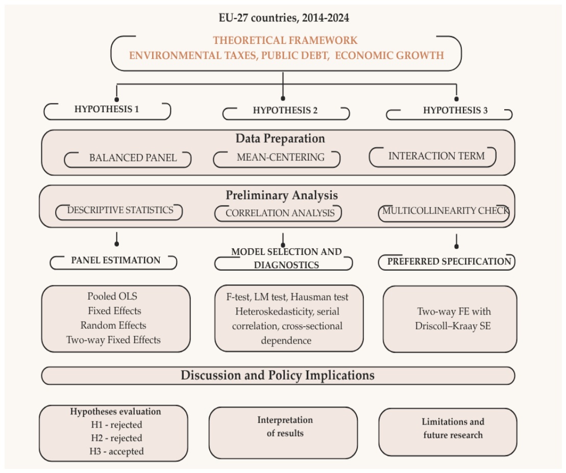
Figure 2.
Marginal Effect of Environmental Taxes on GDP Growth Conditional on Public Debt.
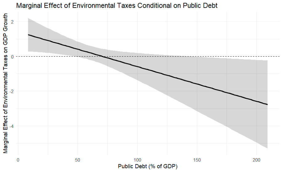
Figure 3.
Conditional Marginal Effects of Environmental Tax Revenue on GDP Growth Evaluated at Country-Average Public Debt Levels.
Figure 3.
Conditional Marginal Effects of Environmental Tax Revenue on GDP Growth Evaluated at Country-Average Public Debt Levels.
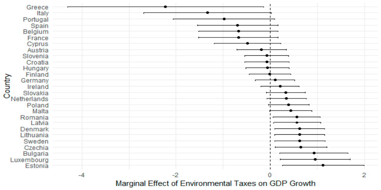

Table 1.
Variables Used in the Empirical Analysis.
| Variable | Abreviation | Description | Unit of measurement | Expected sign | Eurostat dataset | |||
|---|---|---|---|---|---|---|---|---|
| dependent variable | ||||||||
| 1 | Real GDP growth rate at market prices | GDP_Growth | Annual percentage change in real GDP at market prices measured in chain-linked volumes | Chain-linked volumes, percentage change on previous period | tec00115 | |||
| Main independent variable | ||||||||
| 2 | Environmental taxes | Env_Taxes | Environmental tax revenues levied on energy, transport, pollution and resources | Percentage of gross domestic product | ( +/- ) | env_ac_tax | ||
| Moderator independent variable | ||||||||
| 3 | General government gross debt | Debt | General government consolidated gross debt at nominal value | Percentage of gross domestic product | ( - ) | gov_10dd_edpt1 | ||
| Interaction Term | ||||||||
| 4 | Environmental taxes × Public debt | Env_Taxes × Debt | Interaction between environmental taxes and public debt used to test the moderating effect of fiscal conditions | ( - ) | env_ac_tax х gov_10dd_edpt1 | |||
| Control variables | ||||||||
| 5 | Gross fixed capital formation | Invest | Resident producers’ acquisitions less disposals of fixed assets | Percentage of gross domestic product | ( + ) | tec00011 | ||
| 6 | Inflation - Harmonised index of consumer prices | Infl | Annual average rate of change in the Harmonised Index of Consumer Prices (HICP) | Annual average rate of change | ( - ) | prc_hicp_ainr | ||
| 7 | Unemployment | Un_Empl | Persons aged 15–74 who were unemployed, actively seeking work and available to start work | Percentage of population in the labour force 15-74 | ( - ) | une_rt_a | ||
Source: Author’s interpretation.
Table 2.
Descriptive statistics.
| Variable | Mean | Median | Std. dev. | Minimum | Q1 | Q3 | Maximum | Skewness | Excess kurtosis |
|---|---|---|---|---|---|---|---|---|---|
| GDP growth (%) | 2.62 | 2.50 | 3.72 | -10.90 | 1.10 | 4.10 | 24.60 | 0.48 | 5.63 |
| Environmental taxes (% GDP) | 2.60 | 2.50 | 0.80 | 0.85 | 2.03 | 3.01 | 5.62 | 0.62 | 0.19 |
| Government debt (% GDP) | 68.81 | 60.80 | 38.42 | 8.50 | 41.40 | 92.30 | 209.40 | 1.10 | 1.20 |
| Gross fixed capital formation (% GDP) | 21.44 | 21.20 | 4.09 | 11.00 | 19.10 | 23.70 | 53.20 | 1.80 | 13.61 |
| Inflation (HICP. %) | 2.68 | 1.60 | 3.59 | -1.60 | 0.50 | 3.20 | 19.40 | 2.10 | 4.97 |
| Unemployment rate (%) | 7.43 | 6.50 | 3.98 | 2.00 | 5.00 | 8.40 | 26.60 | 2.06 | 5.52 |
Source: Author’s calculation.
Table 3.
Correlation matrix.
| GDP | Environmental taxes | Gross debt | GFCF | HICP | Unemployment | |
|---|---|---|---|---|---|---|
| GDP | 1 | |||||
| Envir.taxes | -0.0820 | 1 | ||||
| Gross debt | -0.1262 | 0.3078 | 1 | |||
| GFCF | 0.0646 | -0.3722 | -0.3751 | 1 | ||
| HICP | 0.0501 | -0.1750 | -0.1631 | 0.1780 | 1 | |
| Unemployment | -0.0929 | 0.3068 | 0.6142 | -0.4253 | -0.3455 | 1 |
Source: Author’s calculation.
Table 4.
VIF values.
| Variable | VIF | Tolerance |
|---|---|---|
| Environmental taxes (centered) | 1.227 | 0.815 |
| Public debt (centered) | 1.801 | 0.555 |
| Environmental taxes × Public debt | 1.389 | 0.720 |
| Gross fixed capital formation | 1.401 | 0.714 |
| Inflation | 1.158 | 0.863 |
| Unemployment | 1.932 | 0.518 |
Source: Author’s calculation.
Table 5.
Diagnostic Tests.
| Test | Model | Null hypothesis | Statistic | p-value | Conclusion |
|---|---|---|---|---|---|
| Breusch–Pagan heteroskedasticity test | FE | Homoskedasticity | BP = 11.027 | 0.088 | Weak evidence of heteroskedasticity |
| Breusch–Pagan heteroskedasticity test | RE | Homoskedasticity | BP = 11.027 | 0.088 | Weak evidence of heteroskedasticity |
| Breusch–Godfrey/Wooldridge serial correlation test | FE | No serial correlation | χ² = 124.350 | < 0.0001 | Serial correlation detected |
| Breusch–Godfrey/Wooldridge serial correlation test | RE | No serial correlation | χ² = 108.830 | < 0.0001 | Serial correlation detected |
| Wooldridge FE serial correlation test | FE | No serial correlation | F = 7.011 | 0.0086 | Serial correlation detected |
| Pesaran CD test | One-way FE | Cross-sectional independence | z = 43.191 | < 0.0001 | Cross-sectional dependence detected |
| Pesaran CD test | RE | Cross-sectional independence | z = 44.939 | < 0.0001 | Cross-sectional dependence detected |
| Pesaran CD test | Two-way FE | Cross-sectional independence | z = −0.821 | 0.412 | No evidence of cross-sectional dependence |
Source: Author’s calculation.
Table 6.
Panel Regression Results and Final Specification.
| Variables | Pooled OLS | Fixed Effects | Random Effects | Two-way FE DK | ||||
|---|---|---|---|---|---|---|---|---|
| β | SE | β | SE | β | SE | β | SE | |
| Environmental Taxes | −0.203 | 0.374 | 1.089* | 0.577 | 0.124 | 0.336 | 0.037 | 0.219 |
| Public Debt | −0.010* | 0.006 | −0.086** | 0.035 | −0.015** | 0.006 | −0.024 | 0.040 |
| Environmental Taxes × Public Debt | 0.001 | 0.005 | −0.022 | 0.023 | −0.005 | 0.007 | −0.020** | 0.009 |
| Investment | 0.005 | 0.085 | −0.066 | 0.045 | −0.028 | 0.046 | 0.005 | 0.094 |
| Inflation | 0.023 | 0.070 | 0.091 | 0.057 | 0.054 | 0.060 | −0.134*** | 0.025 |
| Unemployment | −0.008 | 0.077 | 0.057 | 0.094 | 0.004 | 0.075 | −0.195* | 0.106 |
| Country fixed effects | No | Yes | Random | Yes | ||||
| Year fixed effects | No | No | No | Yes | ||||
| R-squared | 0.019 | 0.057 | 0.016 | 0.072 | ||||
| Model p-value | 0.480 | 0.017 | 0.581 | 0.004 | ||||
| Preferred model | No | No | No | Yes | ||||
Notes: * p < 0.10. ** p < 0.05. *** p < 0.01. Source: Author’s calculation.
Table 7.
Interpretation of Marginal Effects.
| Public debt level | Debt. original scale | Marginal effect of envir. taxes | p-value | Interpretation |
|---|---|---|---|---|
| Low debt −1 SD | 30.39 | 0.804 | 0.015 | Positive and statistically significant |
| Mean debt | 68.81 | 0.037 | 0.866 | Not statistically significant |
| High debt +1 SD | 107.23 | −0.731 | 0.107 | Negative but not statistically significant |
Source: Author’s calculation.
Table 8.
Robustness Checks.
| Specification | Interaction coefficient | Robust SE | p-value |
|---|---|---|---|
| Baseline TWFE–DK | −0.020 | 0.009 | 0.020 |
| Country-clustered SE | −0.020 | 0.020 | 0.318 |
| All regressors lagged one year | −0.013 | 0.006 | 0.037 |
| Excluding 2020–2021 | −0.020 | 0.010 | 0.034 |
Source: Author’s calculation.
Disclaimer/Publisher’s Note: The statements, opinions and data contained in all publications are solely those of the individual author(s) and contributor(s) and not of MDPI and/or the editor(s). MDPI and/or the editor(s) disclaim responsibility for any injury to people or property resulting from any ideas, methods, instructions or products referred to in the content. |
© 2026 by the authors. Licensee MDPI, Basel, Switzerland. This article is an open access article distributed under the terms and conditions of the Creative Commons Attribution (CC BY) license (http://creativecommons.org/licenses/by/4.0/).
Copyright: This open access article is published under a Creative Commons CC BY 4.0 license, which permit the free download, distribution, and reuse, provided that the author and preprint are cited in any reuse.