
Submitted:
14 August 2026
Posted:
17 August 2026
You are already at the latest version
Abstract
Unattended ground sensors (UGS) are passive systems used to detect and classify nearby activity such as the movement of military vehicles or personnel. However, UGS performance is limited in complex environments. This work explores the application of deep learning to classify vehicles as either ‘heavy’ or ‘light’ using seismic, acoustic, and magnetic sensor data collected at varying distances from a road. Two approaches were evaluated: one using manually extracted features from short-time Fourier transforms (STFT), and another using convolutional neural networks trained on time series data. Models were also tested under data partitioning strategies involving either spatial or temporal variation. Data fusion was examined by comparing models that utilized all sensor modalities to those using a single modality. Layer-wise Relevance Propagation was applied to identify informative modalities and frequency components. Models utilizing manually extracted frequency features outperformed time series-based models, with a 3% accuracy difference between the top performers. Spatial-only data partitioning overestimated performance, highlighting the need to incorporate temporally distinct data. The STFT-based fusion model achieved the highest accuracy. Acoustic data, particularly in the frequency range below 100 Hz, was most relevant. Overall, the results demonstrate the effectiveness of manual feature extraction and the importance of careful data partitioning for reliable performance assessment. Future work should explore alternative, finer-tuned neural networks.
Keywords:
vehicle detection
; classification
; compact sensors
; convolutional neural networks
-
What are the main findings?
- Fusion of seismic, acoustic, and magnetic modalities improves model performance
- Acoustic frequencies below 100 Hz are most relevant for vehicle classification
- Tests of generalizability require spatially and temporally independent data splits
- Spectral feature-based models outperform time-series-based models.
1. Introduction
Unattended ground sensing employs passive, covert, battery-powered sensors to detect and identify local activities. The use of unattended ground sensors enables the detection of military vehicles and personnel, offering advantages in tactical intelligence. These systems have been leveraged in the past to provide insight into traffic patterns for strategic planning and early warning systems [1,2,3,4]. However, these systems were often constrained by limited lifetimes and vulnerability to environmental noise. Advances in low Size, Weight, Power, and Cost (SWaP-C) designs have mitigated many of these constraints [1]. Identifying targets in complex environments remains a challenge, motivating the use of artificial intelligence (AI) and machine learning (ML). Compared to traditional rule-based algorithms, ML approaches are more flexible and benefit from open-source frameworks. Deep learning, in particular, has emerged as a powerful subset of ML, and neural networks have demonstrated state-of-the-art performance in vehicle classification across sensor modalities, including acoustic, magnetic, and seismic [5].
1.1. Related Work
Limited research has explored how multimodal sensing can be effectively combined with deep learning to improve vehicle classification. Most prior studies have relied on single-modality inputs, including acoustic [6,7,8], seismic [9,10], or magnetic signals [11,12,13], with sensors typically placed close to the road. Many approaches also depend on static feature representations extracted from short signal segments and classified with multilayer perceptrons [14,15,16,17,18,19,20,21]. Recent work has introduced other deep learning methods capable of capturing temporal dependencies in signals. For example, Thu et al. used CNNs with mel-frequency cepstral coefficients from acoustic frames to achieve 86.3% accuracy in classifying between buses, cars, motorcycles and trucks [6], while Jin et al. proposed log-scaled frequency cepstral coefficients for seismic signals, reaching 91.9% accuracy in classifying between an Assault Amphibious Vehicle and a dragon wagon [9]. Beyond handcrafted features, Wang et al. demonstrated that CNNs trained directly on raw seismic recordings could surpass feature-engineered methods, achieving 95.5% accuracy distinguishing between pedestrians, wheeled, and tracked vehicles with their VibCNN architecture [10].
Hybrid models have also been explored. Kurowski et al. showed that incorporating temporal context through variable-length acoustic frames improved CNN performance for distinguishing cars from heavy vehicles [22], while Luo et al. and Mohine et al. employed CNN–LSTM hybrids for acoustic vehicle classification of cars, buses, and trucks [7,8]. For magnetic sensing, Sarcevic et al. relied on hand-engineered features with limited performance in a classification task for cars, motorcycles, trucks, and buses, whereas Kolukisa et al. applied LSTMs to raw magnetic sequences, achieving similar accuracies classifying between light, medium, and heavy-weight vehicles [12,13]. Overall, prior research demonstrates the growing use of deep learning for vehicle classification but remains constrained by single-modality designs, near-road sensor placements, and reliance on feature engineering.
1.2. Current Research
The primary objective of this research is to accurately distinguish between heavy and light vehicles using data collected from a multimodal unattended ground sensing system that recorded seismic, acoustic, and magnetic signals. Convolutional neural networks were evaluated with both time series and frequency-domain feature inputs. A fusion model was developed to integrate information across the three sensor modalities. To assess generalizability, model classification performance was examined under two partitioning strategies: separation by transverse sensor placement and separation by temporally distinct vehicle passes. Finally, Layer-wise Relevance Propagation was applied to frequency feature-based networks to provide insight into which frequencies and signal modalities were most relevant for vehicle classification.
Vehicle passes were segmented from background activity using a triggering algorithm designed to approximate real-time detection. The resulting segments were preprocessed using two approaches: feature extraction via Short-Time Fourier Transform (STFT) and downsampling to reduce noise and input size. The processed data were partitioned into training, validation, and testing sets using both temporal and spatial strategies. Convolutional neural networks were then trained using either single-modality inputs or fused multimodal inputs.
The remainder of this document is organized as follows: Section II details the data and methodology, Section III presents the results and their implications, and Section IV concludes with key findings, study limitations, and directions for future work.
2. Methodology
This section outlines the methodology used in this study. It begins with an overview of the dataset, which includes the collection of acoustic, seismic, and magnetic signals from both heavy and light vehicles. Next, the triggering and segmentation process used to isolate vehicle passes is described, followed by preprocessing steps and the training and evaluation of convolutional neural networks. The overall workflow is shown in Figure 1.
2.1. Data Details
The data used in this study were collected in 2020 as part of an exercise sponsored by the Defense Threat Reduction Agency (DTRA). During the exercise, vehicles of two specific classes were driven along a pre-planned route in a controlled manner following an experiment plan. The vehicle classes were defined as heavy and light. The heavy class comprised two test articles, while the light class consisted of two military trucks (M923 and M934). Representative vehicles are shown in Figure 2 and Figure 3. The military trucks weighed approximately 5 tons, while the heavy test articles were equivalent to a 500-ton mobile crane. Data collection was conducted over two days, yielding 40 labeled vehicle passes on Day 1 and 38 on Day 2. With four sensor systems operating on Day 1 and five on Day 2, the combined total number of recordings was 350.
Each vehicle pass involved moving from a designated start point along an approximately straight 3-mile road segment to an end point. Upon reaching the end, the vehicle was driven back to the start, constituting a separate return pass. Summarized in Table 1 are the details of the number of passes of each vehicle type and the speed of the vehicles. It can be seen that there are passes conducted at a variety of speeds and vehicle types on each day of the exercise.
The sensor systems deployed during data collection were equipped with a three-axis geophone (seismic), an array of three pre-polarized, omnidirectional condenser microphones spaced 120° apart (acoustic), and a three-axis fluxgate magnetometer (magnetic). When combined into a single sensor package, these Seismic, Acoustic, and Magnetic sensor systems are referred to as SAMs. All channels were sampled at 8533.33 Hz and resampled to an integer rate of 8533 Hz for analysis. The microphones exhibited an approximately flat free-field response at 0° incidence between 10 Hz and 8 kHz, with variations within ±1 dB. The seismic sensors were three-vector geophones with a flat response up to 1 kHz and attenuation below 4.5 Hz. The magnetic sensors were three-vector fluxgate magnetometers with a flat response from 0 Hz to 1 kHz and deviations within ±5% at a 1 kHz peak.
The number and placement of SAMs varied between the two days of data collection. On Day 1, four SAMs were deployed as shown in Figure 4, and on Day 2, five SAMs were deployed as shown in Figure 5. In addition to sensor data, GPS coordinates for both sensors and vehicles were recorded. The vehicle’s GPS tracks, initially provided as latitude, longitude, and elevation, were converted into relative distances from each sensor as a function of time allowing the times of closest approach to be identified.
2.2. Vehicle Pass Segmentation
A vehicle detection algorithm was developed to simulate real-time data processing and enable vehicle pass segmentation. Because vehicle classification is the primary focus of this work, the detection algorithm was designed with two objectives: all vehicle-associated intervals must be included in the machine learning dataset, and these intervals must be segmented appropriately for labeling. These objectives limit the algorithm’s applicability to clearly distinguished vehicles as opposed to closely spaced convoys where signals from multiple vehicles overlap.
The algorithm leveraged the seismic signal magnitude, as shown in Equation 1, to simulate the activation of the other sensors in a system.
Within this equation, , , and correspond to the raw data recorded by each directional channel of the geophone. Seismic phenomenology was selected because it is less susceptible to environmental noise. Seismic signals also propagate farther, and their intensity decays more slowly than acoustic and magnetic signals [23]. In contrast, the acoustic signals generally exhibit higher noise levels and are prone to false positives.
The seismic magnitude data is aggregated along the time axis using one-second non-overlapping block averages; each block contains 8,533 samples. Following block averaging, two exponential moving averages (EMA) are calculated: a short-term average (STA) and a long-term average (LTA). These EMA are calculated according to
where is the smoothing factor, is the value at the current timestep, and and are the exponential moving average values at the current and previous timesteps.
At each one-second timestep, the block average from each second updates the STA. The LTA is updated only when the STA/LTA ratio falls below a user-defined threshold. A trigger is declared when the STA/LTA ratio exceeds this threshold and remains in effect until the ratio returns to below the threshold. This method is widely used for earthquake detection and has also been adapted for vehicle detection with other phenomenologies [24,25,26,27].
Parameter values were selected based on the algorithm’s ability to detect and segment all vehicle passes. The EMAs are characterized by their smoothing factors, which are derived from specified window sizes. The relationship between the smoothing factor and window size is
An EMA with the calculated smoothing factor approximates a simple moving average (SMA) of length N, where N is the number of data points within a specified window size.
The triggering algorithm can be summarized as follows for each non-overlapping one-second block of data:
- 1.
- Compute the seismic magnitude and calculate its mean value (feature extraction).
- 2.
- 3.
- Calculate the ratio between the short-term EMA and the long-term EMA.
- 4.
- If this ratio is equal or below a user-defined threshold, update the long-term EMA with the current mean.
- 5.
- If the ratio exceeds the threshold, do not update the long-term EMA and flag this time block as potentially containing a vehicle.
- 6.
- Repeat Steps 1–5 until the end of the data stream.
The STA and LTA window durations were set to 20 seconds and 200 seconds, respectively. Trigger thresholds from 1.0 to 2.0 in increments of 0.1 were tested for each sensor system. A vehicle pass was considered captured if visual inspection confirmed that the majority of the signal, including its peak, was within a trigger window. The final trigger threshold selected was 1.4. The parameter settings were chosen to segment and capture all the vehicle passes.
Each triggering window, illustrated in Figure 6, was labeled for supervised machine learning using the time of closest approach (TCA). The TCA is the timestamp at which the distance between the vehicle’s GPS track and the sensor’s GPS location is at its minimum. Windows containing a vehicle’s TCA were one-hot encoded into three categories: heavy, light, or vehicle absent. Following this, data associated with vehicle absence was removed entirely. After triggering and labeling, the resulting dataset contained only intervals where either a heavy or light vehicle was near the sensor. Additional details related to the application of the triggering algorithm specific to this dataset are provided in Appendix A.1.
2.3. Pre-Processing
The number of data streams was reduced before model training to eliminate redundancies and compress the data. For the acoustic signal, only the second microphone was retained as the signal-to-noise ratio for the other microphones was lower for some systems. The X and Y outputs of the geophone and magnetometer were combined per modality using a magnitude calculation. This preprocessing resulted in five data streams: acoustic microphone 2, seismic Z, seismic XY magnitude, magnetic z, magnetic XY magnitude. These data streams were further processed using two approaches to compare manual and automatic feature extraction. Data preprocessing for manual extraction involved transforming the time series data into frequency features, whereas preprocessing for automatic extraction consisted solely of downsampling, allowing the model to learn directly from the time series data.
2.3.1. Short Time Fourier Transform
Feature extraction was performed on each of the five data streams using a Short Time Fourier Transform (STFT) via SciPy’s stft function. Scipy’s stft parameter settings are detailed in Table 2.
The magnitude of the complex STFT coefficients was computed, normalized with the sum of the coefficients, and log-transformed. The purpose of this normalization is to mitigate the impact of individual sensor gains on the power spectra. The feature vector for each one-second data segment was reduced by discarding the DC component and frequency components above 609 Hz for each of the five data streams. The DC component was discarded to make the analysis more generalizable to sensor distance from the road. The 1 Hz seismic components were also discarded because the geophones exhibited significant attenuation of the signal at low frequencies. The 609 Hz upper bound matches the Nyquist rate of the downsampled data described in the next section and is above the key frequencies that literature suggests are relevant for vehicle classification [28,29,30]. This approach enables better comparison between methods.
2.3.2. Signal Downsampling
The raw time series data were downsampled before being input into the convolutional neural networks. Downsampling reduces high-frequency noise and the volume of data to be processed. Downsampling involves two main steps: applying an anti-aliasing filter and decimation to reduce the sampling rate. An anti-aliasing filter attenuates high frequencies to prevent aliasing during downsampling. The filter’s cutoff frequency must be at or below the new Nyquist frequency. A decimation factor of 7 was used, yielding a new sample rate of 1219 Hz and a Nyquist frequency of 609 Hz. Each 1-second segment (1219 timesteps) is treated as an independent observation or instance. The decimation factor of 7 was chosen as it is a convenient factor of the original sampling rate, resulting in a new integer sample rate.
A Bessel filter was selected to avoid signal distortion in the time domain. Bessel filters provide a maximally linear phase response and preserve waveform integrity better than other filter types (Butterworth, Chebyshev, Elliptic) [31]. Filter parameter values are listed in Table 3.
The Bessel function provides the necessary filter coefficients, which are then applied using SciPy’s lfilter. lfilter preserves causality, simulating real-time filtering behavior. Its inputs are the Bessel coefficients and a data array. After filtering, decimation is performed by retaining every 7th data point. This filtering and decimation procedure resulted in downsampled time series data.
2.4. Data Partitioning
In two independent approaches designed to evaluate both spatial and temporal generalizability of the machine learning models, the data were partitioned into training, validation, and test sets using two strategies, summarized in Table 4. The first approach involves spatially separating the data. The training set comprises data from sensors placed 25, 50, and 125 meters from the road (i.e., Day 1: SAM 2, 4, and 6; and Day 2: SAM 1, 2, 5, and 6). The validation set comprises data from a sensor placed 75 meters away from the road (Day 1, SAM 3), and the test set from a sensor at 100 meters from the road (Day 2, SAM 4). The reader is referred to the sensor layouts for both days shown in Figure 4 and Figure 5. The second approach involves temporal separation of data, i.e., the training and testing set does not include data from sensors recording the same vehicle pass. The training data contains data only from Day 2. The validation and test sets were formed by splitting the vehicle passes from Day 1 based on longitudinal sensor placement. The validation set contains the vehicle passes as observed by SAM 2 and 3, while the test set contains the vehicle passes as observed by SAM 4. This data split utilizes the longitudinal spacing between these three sensors, ensuring no temporal overlap in the recordings of a vehicle pass obtained from multiple sensors as discussed further in Section 3. SAM 6 was not used for the temporal split due to signal overlap with SAM 3, 4, and 6. The quantity of data observations assigned to the training, validation and test sets for each partitioning strategy is provided in Appendix A.2.
2.5. Model Architectures and Evaluation
Convolutional neural networks were trained based on the data split strategies described above. In total, 10 models were developed: two using the spatial separation approach and eight using the temporal separation approach. The two models trained using the spatially separated data utilized either manually extracted acoustic STFT features or the downsampled acoustic time series. A comparison between a fusion of phenomenologies and individual phenomenologies was not explored; only the acoustic phenomenology was utilized. This portion of the study, employing the spatial partitioning strategy, indicated that the training, validation, and test sets were highly similar, leading to an overestimation of model performance. In contrast, the second data partitioning approach (temporal partitioning) was explored in greater detail, including a comparison between manual and automatic feature extraction methods, as well as between single phenomenology and fusion approaches.
Each model is similar in architecture. The output layers consist of a single neuron with a ‘sigmoid’ activation function. The preceding layers were modified based on the input and the model’s capacity. The capacity of each model was initially increased to overfit the training set, and then regularization, in the form of dropout and L2 regularization, was introduced to prevent overfitting. Each model’s architecture was manually tuned using the validation set, and the model with the lowest validation loss was retained for evaluation with the test set. The hyperparameter values considered for the CNN are summarized in Table 5.
The models with individual phenomenological inputs (e.g., those that utilize only acoustic, seismic, or magnetic data) share a similar structure. The general model architecture consists of an input layer, followed by several stacks of convolutional layers, a global max pooling layer, a dense layer, and an output neuron.
For models using a fusion of phenomenologies, separate feature extraction branches were constructed. These branches are similarly composed of stacks of convolutional layers and a global max pooling layer with identical hyperparameters as those of the single phenomenology models. The outputs from these branches were concatenated and passed to a penultimate dense layer before the output neuron. Architecture diagrams for each model can be found in Appendix A.3.
Training and validation losses were calculated using the binary cross-entropy loss function. The performance measures reported include balanced accuracy, recall, precision, and Matthews correlation coefficient (MCC).
2.6. Model Explainability
Layer-wise Relevance Propagation (LRP) was used to provide model interpretability, implemented via the iNNvestigate toolbox [32]. LRP offers several propagation rules, including the Basic (LRP-0), Epsilon (LRP-), and Gamma (LRP-) rules [33]. The Basic rule assigns relevance in direct proportion to each input’s contribution to a neuron’s activation. The Epsilon rule introduces a small stabilizing parameter, , to suppress noisy or contradictory contributions. The Gamma rule modifies the redistribution to emphasize positive contributions by incorporating a tunable parameter . To avoid introducing additional parameters, the “Basic rule" (LRP-0) was used. The test set was analyzed based on vehicle class, and relevance maps were averaged within each class to generate class-specific heatmaps. LRP was applied to the networks using frequency-transformed data to identify frequency bands that are important for the heavy and light classification task. LRP was not applied directly to the networks using raw time series inputs, as they represent sequential timesteps rather than spectrally meaningful input features.
3. Results and Discussion
This section presents the results obtained for each model. As outlined in the Methodology, the dataset was partitioned to evaluate the impact of sensor distance from the road and the effect of temporal separation between training and test data. In addition, two data preparation approaches were tested: manual feature extraction using the STFT and automatic feature extraction using downsampled data. Each model and its predictions are analyzed to assess the importance of specific frequencies and phenomenologies. A summary of the results is shown in Table 6.
3.1. Comparing Partitioning Strategies
As shown in Table 6, the model’s performance under the spatial partitioning strategy was exceptionally high, with the model utilizing acoustic STFT features achieving a balanced accuracy of 99%. In contrast, the best-performing model under the temporal partitioning scheme achieved only 93% balanced accuracy, a 6% decrease.
There is a limitation to the generalizability of these results for the spatial partitioning method. Although the spatial partitioning strategy involved data from distinct sensors at different distances from the road, each of those sensors recorded each vehicle pass event which means they were recording the same event from different perspectives. Because of spatial partitioning, this same event recorded at two different sensors could be split between the the training data and the test data. For example, data from SAM 2 was included in the training set, while simultaneously recorded data of the same vehicle pass event recorded by SAM 4 was used for testing since it was located at a different spatial position further away from the road. This partitioning method may result in the model performing better on test-set sensor-recorded patterns of the same event used for training - which could lead to an overestimate in model performance in future data. Since the testing procedure does not prevent the same event from being learned during training and evaluated during test, it is methodologically unsound to interpret strong performance under this partitioning method as evidence of generalizability to new data.
3.2. Comparing Preprocessing Approaches
In general, feature extraction using the STFT outperformed models trained directly on raw time series data across all evaluation metrics. Under the temporal partitioning scheme, the model using STFT features from all three phenomenologies achieved the highest balanced accuracy, 93%. Performance was closely followed by the models trained with acoustic and seismic STFT features. In comparison, the best-performing time series model, which incorporated all three modalities, achieved only 90% balanced accuracy. Nevertheless, time-series neural networks may still be advantageous in scenarios where the combined computational cost of spectral feature extraction and a convolutional neural network is greater than that of a model capable of directly learning from minimally processed signals.
3.3. Individual Modality and Fusion Models
Fusion models outperformed individual modality models. The STFT fusion model, which incorporates all three phenomenologies, achieved the highest balanced accuracy, followed closely by the acoustic and seismic STFT models. The magnetic modality based models performed the worst, achieving results on par with random guessing. The time series fusion model also outperformed individual time series models, but still lagged behind the STFT fusion models.
The residuals of the best-performing STFT fusion model were analyzed to investigate error patterns. Figure 7 shows the residuals plotted as a function of scaled time for each vehicle pass in the test set. The model made more errors on light vehicle passes. Errors tended to cluster within individual passes, suggesting temporal correlation typical of time series data. Many occurred near the beginning or end of the vehicle’s pass windows.
An alternating error pattern was observed between the M934 and M923 passes, corresponding to the vehicles completing forward and reverse passes. When traveling in the forward direction (from start to endpoint), errors were more frequent at the beginning of the pass. Conversely, in the reverse direction, errors tended to occur near the end. This effect was especially prominent for the M923, as shown in Figure 8.
Vehicle speed did not significantly affect classification accuracy. Light vehicle passes conducted at 24 km/h (passes 1–12) and 40 km/h (passes 13–24) exhibited similar misclassification rates. Heavy vehicle passes at both speeds also showed no substantial difference in performance. For heavy vehicles, the alternating forward–reverse error pattern was less pronounced, suggesting that the model detected the presence of heavy vehicles regardless of travel direction or speed.
3.4. Relevant Features and Modalities
Layer-wise relevance propagation (LRP) was employed to interpret the best-performing model, specifically the STFT fusion model that incorporates all three phenomenologies. Class-specific feature importance heatmaps (Figure 9 and Figure 10) visualize the relevance of input features. The most relevant features were acoustic frequencies below 100 Hz, in the 40–46 Hz and 64–70 Hz ranges. Seismic channels contributed little, with sparse relevance distributed across broadband frequencies up to 400 Hz. Magnetic channels appeared largely irrelevant, consistent with the poor performance of the magnetic-only model reported earlier.
4. Conclusions and Future Work
4.1. Conclusions
This study evaluated deep learning approaches for the binary classification of heavy and light vehicles using seismic, acoustic, and magnetic sensor data. Manual feature extraction using the STFT consistently outperformed models that relied on learned feature representations from downsampled time series. While fusion-based time series models achieved on-par performance when incorporating all three phenomenologies, their balanced accuracy (90%) remained below that of the best-performing STFT-based model (93%), and their recall and Matthews correlation coefficient were also lower.
The choice of data partitioning strategy also affected the evaluation of model generalizability. Splitting data solely by spatial sensor placement produced overestimations of performance due to the similarity of signals recorded during concurrently recorded vehicle passes. A model trained on acoustic STFT features achieved a balanced accuracy of 99.1% under the spatial partitioning strategy. However, when evaluated under a temporally distinct split, its accuracy decreased to 93.0%, a drop of approximately 6%. Multimodal data fusion offered only marginal gains.
The fusion of acoustic, seismic, and magnetic features produced performance comparable to acoustic-only models, with accuracy improving by only 1%. The precision, recall, and Matthews correlation coefficient improved only by up to 0.02. Layer-wise Relevance Propagation confirmed that acoustic features dominated the decision-making process, with seismic features and magnetic features contributing negligibly. While seismic data was useful for triggering vehicle detection, their value for classification was limited.
Finally, explainability analysis revealed which frequency components were most relevant for classification. For acoustic inputs, the dominant features lie in the 40–46 Hz and 64–70 Hz ranges for heavy and light vehicles, respectively.
In summary, the findings indicate that acoustic features, particularly in the low-frequency range, are most relevant for vehicle classification. STFT-based preprocessing yields better model performance compared to automatic feature learning, and temporally distinct data partitioning is crucial to obtain accurate estimates of generalization.
4.2. Future Work
There are several potential pathways for future work, which can be broadly categorized as either data collection or data analysis (post-collection). The following sections detail suggestions for future work in both categories.
4.2.1. Data Collection
Future data collection efforts could enhance model generalizability by increasing diversity in both environmental conditions and sensor configurations. In particular, conducting recordings across multiple days would allow each day’s data to serve as an independent training, validation, or testing set. Increasing the number of vehicle passes, deploying additional sensor systems, and varying sensor placements would further contribute to a dataset that better captures variability in vehicles and background noise conditions. When resources are limited, as in the present study (two days of recording, a three-mile road, and six sensors available per day), sensor placement can be optimized to reduce temporal overlap. The longitudinal spacing between sensors should be determined by vehicle speed. Slower vehicles allow closer sensor placement, while faster vehicles require greater separation to ensure that recordings remain distinct. For example, the 1,800-meter spacing between SAM 4 and SAM 2 on Day 1 was sufficient to prevent overlap at a speed of 25 mph. Additionally, the placement of transverse sensors should be varied to introduce diversity in the signal-to-noise present in the data. Using the present study as an example, three sensors could be positioned at 25, 75, and 125 meters from the road at one end of the route, while another three could be placed at 50, 100, and 150 meters from the road at the other end of the route. Ultimately, conducting data collection over multiple days, with each day dedicated to a distinct sensor configuration, would most effectively eliminate overlap and yield independent datasets.
4.2.2. Data Analysis
Future analysis could benefit from approaches tailored to the characteristics of each sensor phenomenology. For acoustic, seismic, and magnetic signals, applying different frequency cutoffs or temporal downsampling settings may better leverage their physical propagation properties. In particular, greater attention should be given to the seismic and magnetic modalities. For multichannel seismic signals, adaptive polarization filtering may be more effective in enhancing the signal-to-noise ratio than conventional frequency-based filtering [34]. For magnetic signals, which are dominated by low-frequency and temporally diffuse components, models that incorporate temporal context may outperform smaller frame-based approaches. Leveraging longer time windows would enable the model to capture evolving magnetic signatures as vehicles pass by the sensors. Beyond preprocessing, improvements may also be achieved through expanded hyperparameter searches and alternative neural architectures.
Conflicts of Interest
The authors declare that they have no known competing financial interests or personal relationships that could have appeared to influence the work reported in this paper.
Appendix A
Appendix A.1. Triggering Algorithm and Segmentation
The following section contains additional information about the triggering algorithm. The seismic magnitude data is aggregated along the time axis using one-second non-overlapping block averages; each block contains 8,533 samples. Alternative feature extraction methods, such as energy within specific frequency bands, power, variance, or autocorrelation, could be used instead. Figure A1 shows an example of the data before and after aggregation.
Figure A1.
Signal Feature Extraction. The seismic magnitude data (a) is aggregated via block averaging. The aggregated signal (b) is processed to determine whether a vehicle is present or not.
Figure A1.
Signal Feature Extraction. The seismic magnitude data (a) is aggregated via block averaging. The aggregated signal (b) is processed to determine whether a vehicle is present or not.
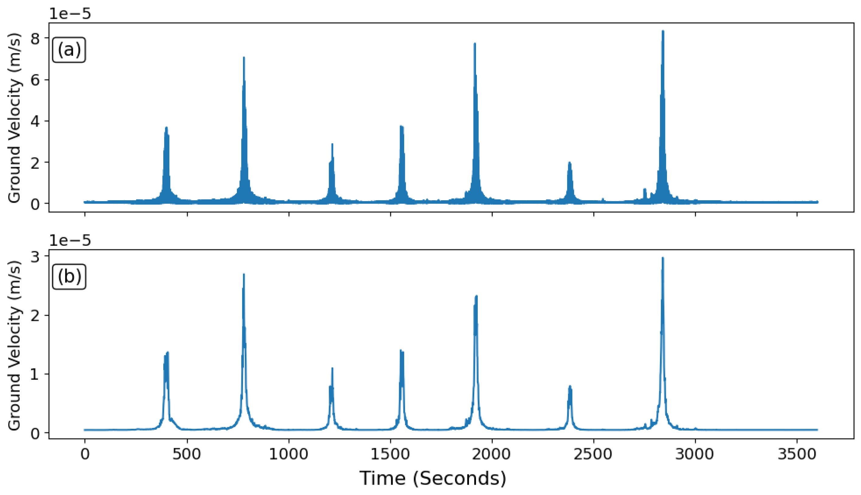
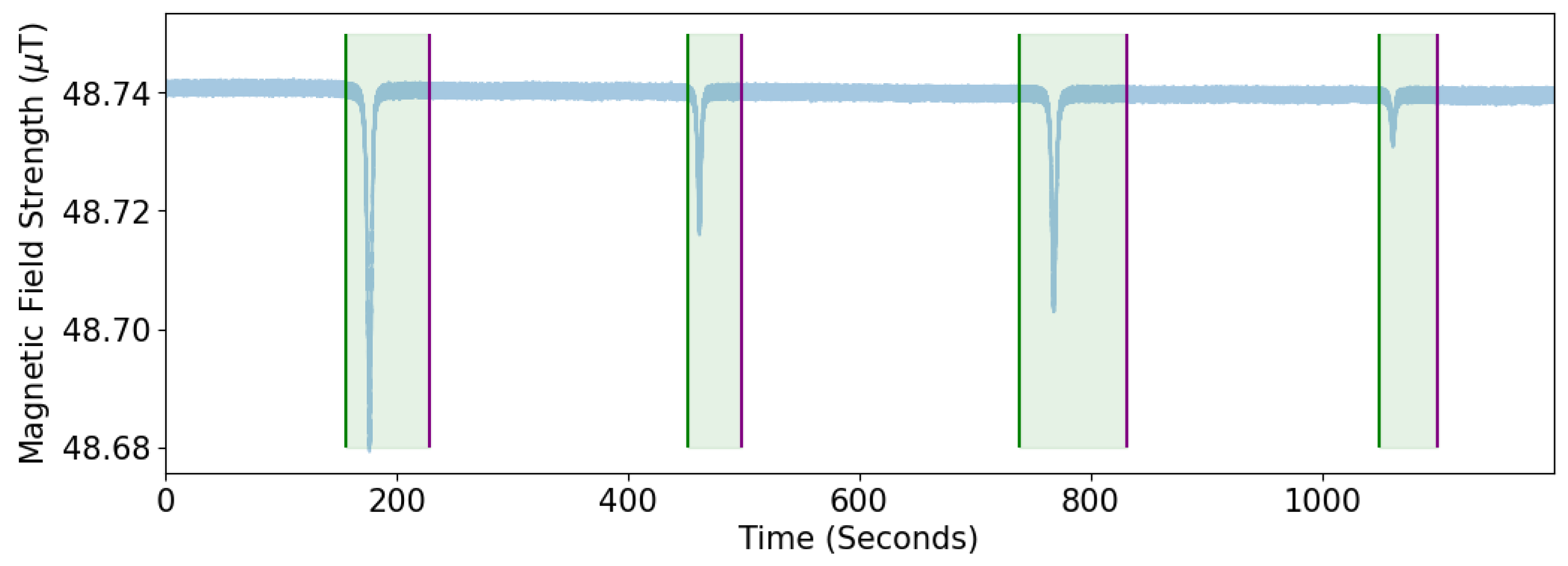
Following feature extraction (block averaging), two exponential moving averages are calculated: a short-term average (STA) and a long-term average (LTA). At each one-second timestep, the feature from each block updates the STA. The LTA is updated only when the STA/LTA ratio falls below a user-defined threshold. A trigger is declared when the STA/LTA ratio exceeds this threshold and persists until the ratio drops back below the threshold. The windows produced by the triggering algorithm were applied to the other phenomenologies, as shown by Figure A2, Figure A3, and Figure A4.
Figure A2.
Trigger Windows Applied for Seismic Phenomenology. The order of the passes shown here consists of a heavy vehicle, followed by a light vehicle, another heavy vehicle, and finally a light vehicle. While the windows capture the majority of each pass, they are not centered.
Figure A2.
Trigger Windows Applied for Seismic Phenomenology. The order of the passes shown here consists of a heavy vehicle, followed by a light vehicle, another heavy vehicle, and finally a light vehicle. While the windows capture the majority of each pass, they are not centered.
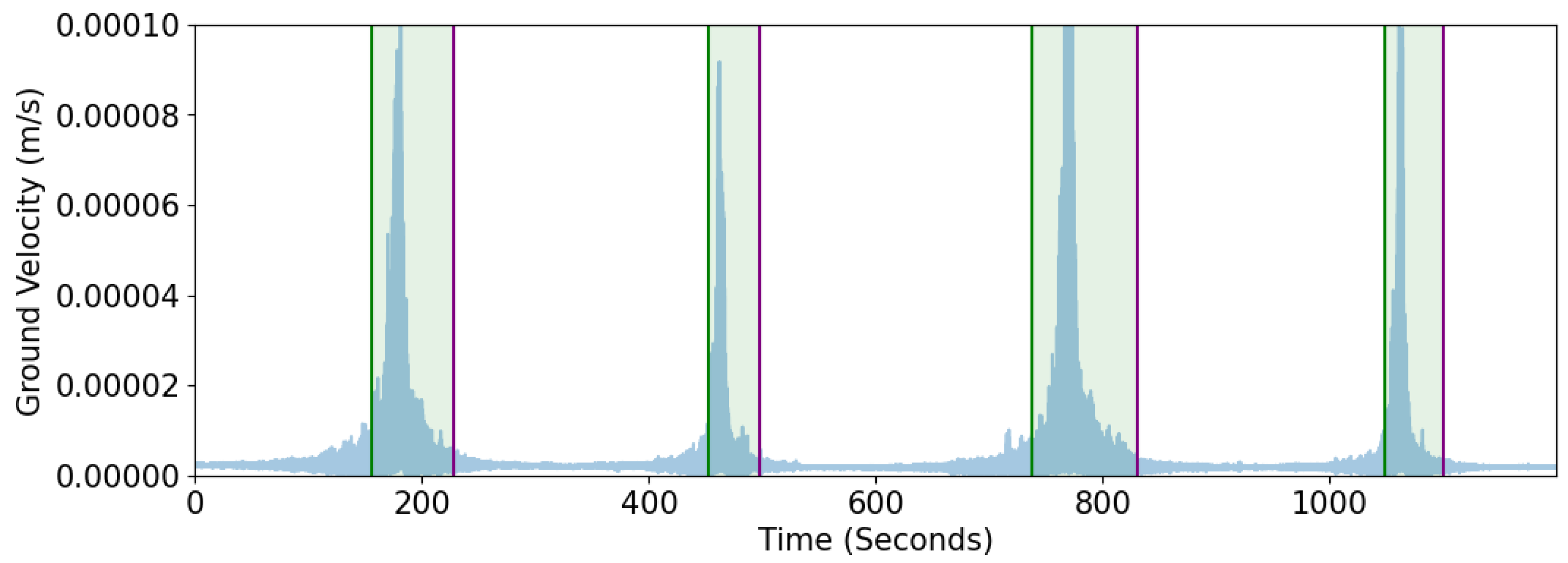
Figure A3.
Trigger Windows Applied for Acoustic Phenomenology. The order of the passes shown here consists of a heavy vehicle, followed by a light vehicle, another heavy vehicle, and finally a light vehicle. While the windows capture the majority of each pass, they are not centered.
Figure A3.
Trigger Windows Applied for Acoustic Phenomenology. The order of the passes shown here consists of a heavy vehicle, followed by a light vehicle, another heavy vehicle, and finally a light vehicle. While the windows capture the majority of each pass, they are not centered.
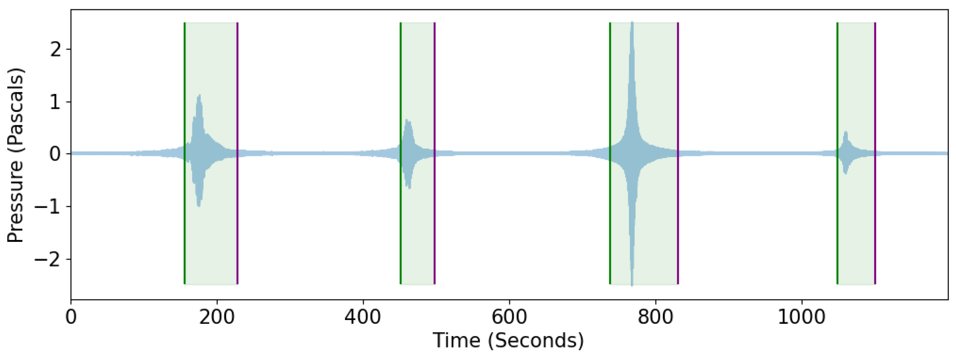
Figure A4.
Trigger Windows Applied for Magnetic Phenomenology. The order of the passes shown here consists of a heavy vehicle, followed by a light vehicle, another heavy vehicle, and finally a light vehicle. While the windows capture the majority of each pass, they are not centered.
Figure A4.
Trigger Windows Applied for Magnetic Phenomenology. The order of the passes shown here consists of a heavy vehicle, followed by a light vehicle, another heavy vehicle, and finally a light vehicle. While the windows capture the majority of each pass, they are not centered.
Appendix A.2. Data Partitioning: Class Breakdowns

Table A1.
Spatial Separation: Training, Validation, and Testing Class Breakdown.
| Data Set | Heavy Class Observation Count | Light Class Observation Count | Total |
|---|---|---|---|
| Training | 14775 (55 %) | 12332 (45 %) | 27107 |
| Validation | 1438 (53 %) | 1255 (47 %) | 2693 |
| Testing | 1631 (57 %) | 1208 (43 %) | 2839 |
Table A2.
Temporal Separation: Training, Validation, and Testing Class Breakdown.
| Data Set | Heavy Class Observation Count | Light Class Observation Count | Total |
|---|---|---|---|
| Training | 8927 (56 %) | 7095 (44 %) | 16022 |
| Validation | 4329 (54 %) | 3717 (46 %) | 8046 |
| Testing | 2465 (53 %) | 2180 (47 %) | 4645 |
Appendix A.3. CNN Architectures
The architecture designs for the acoustic-only and fusion models, which utilize either STFT features or time series inputs, are shown in Table A3, Table A4, Table A5 and Table A6.
Table A3.
Architecture of the Acoustic Time-Series CNN Model.
| Layer (type) | Input Shape | Output Shape |
|---|---|---|
| InputLayer | (1219, 1) | (1219, 1) |
| Conv1D | (1219, 1) | (610, 8) |
| Conv1D | (610, 8) | (204, 8) |
| Conv1D | (204, 8) | (68, 16) |
| Conv1D | (68, 16) | (23, 16) |
| SpatialDropout1D | (23, 16) | (23, 16) |
| Conv1D | (23, 16) | (8, 32) |
| Conv1D | (8, 32) | (3, 32) |
| SpatialDropout1D | (3, 32) | (3, 32) |
| GlobalMaxPooling1D | (3, 32) | (32) |
| Dense | (32) | (16) |
| Dense | (16) | (1) |
Table A4.
Architecture of the Acoustic STFT CNN Model.
| Layer (type) | Input Shape | Output Shape |
|---|---|---|
| InputLayer | (609, 1) | (609, 1) |
| Conv1D | (609, 1) | (305, 8) |
| Conv1D | (305, 8) | (153, 8) |
| SpatialDropout1D | (153, 8) | (153, 8) |
| Conv1D | (153, 8) | (51, 16) |
| Conv1D | (51, 16) | (17, 16) |
| SpatialDropout1D | (17, 16) | (17, 16) |
| Conv1D | (17, 16) | (6, 32) |
| Conv1D | (6, 32) | (2, 32) |
| SpatialDropout1D | (2, 32) | (2, 32) |
| GlobalMaxPooling1D | (2, 32) | (32) |
| Dense | (32) | (4) |
| Dense | (4) | (1) |
Table A5.
Architecture of the Fusion Time-Series CNN Model.
| Layer (type) | Input Shape | Output Shape |
|---|---|---|
| Acoustic InputLayer | (1219, 1) | (1219, 1) |
| Conv1D | (1219, 1) | (610, 8) |
| Conv1D | (610, 8) | (305, 8) |
| Conv1D | (305, 8) | (153, 16) |
| Conv1D | (153, 16) | (77, 16) |
| SpatialDropout1D | (77, 16) | (77, 16) |
| Conv1D | (77, 16) | (39, 32) |
| Conv1D | (39, 32) | (20, 32) |
| SpatialDropout1D | (20, 32) | (20, 32) |
| GlobalMaxPooling1D | (20, 32) | (32) |
| Seismic InputLayer | (1219, 2) | (1219, 2) |
| Conv1D | (1219, 2) | (610, 8) |
| Conv1D | (610, 8) | (305, 8) |
| Conv1D | (305, 8) | (153, 16) |
| Conv1D | (153, 16) | (77, 16) |
| SpatialDropout1D | (77, 16) | (77, 16) |
| Conv1D | (77, 16) | (39, 32) |
| Conv1D | (39, 32) | (20, 32) |
| SpatialDropout1D | (20, 32) | (20, 32) |
| GlobalMaxPooling1D | (20, 32) | (32) |
| Magnetic InputLayer | (1219, 2) | (1219, 2) |
| Conv1D | (1219, 2) | (610, 8) |
| Conv1D | (610, 8) | (305, 8) |
| Conv1D | (305, 8) | (153, 16) |
| Conv1D | (153, 16) | (77, 16) |
| SpatialDropout1D | (77, 16) | (77, 16) |
| Conv1D | (77, 16) | (39, 32) |
| Conv1D | (39, 32) | (20, 32) |
| SpatialDropout1D | (20, 32) | (20, 32) |
| GlobalMaxPooling1D | (20, 32) | (32) |
| Concatenate | (32, 32, 32) | (96) |
| Dense | (96) | (8) |
| Dense | (8) | (1) |
Table A6.
Architecture of the Fusion STFT CNN Model.
| Layer (type) | Input Shape | Output Shape |
|---|---|---|
| Acoustic InputLayer | (609, 1) | (609, 1) |
| Conv1D | (609, 1) | (305, 16) |
| Conv1D | (305, 16) | (153, 16) |
| Conv1D | (153, 16) | (51, 32) |
| Conv1D | (51, 32) | (17, 32) |
| SpatialDropout1D | (17, 32) | (17, 32) |
| Conv1D | (17, 32) | (6, 64) |
| Conv1D | (6, 64) | (2, 64) |
| SpatialDropout1D | (2, 64) | (2, 64) |
| GlobalMaxPooling1D | (2, 64) | (64) |
| Seismic InputLayer | (608, 2) | (608, 2) |
| Conv1D | (608, 2) | (304, 16) |
| Conv1D | (304, 16) | (152, 16) |
| Conv1D | (152, 16) | (51, 32) |
| Conv1D | (51, 32) | (17, 32) |
| SpatialDropout1D | (17, 32) | (17, 32) |
| Conv1D | (17, 32) | (6, 64) |
| Conv1D | (6, 64) | (2, 64) |
| SpatialDropout1D | (2, 64) | (2, 64) |
| GlobalMaxPooling1D | (2, 64) | (64) |
| Magnetic InputLayer | (609, 2) | (609, 2) |
| Conv1D | (609, 2) | (305, 16) |
| Conv1D | (305, 16) | (153, 16) |
| Conv1D | (153, 16) | (51, 32) |
| Conv1D | (51, 32) | (17, 32) |
| SpatialDropout1D | (17, 32) | (17, 32) |
| Conv1D | (17, 32) | (6, 64) |
| Conv1D | (6, 64) | (2, 64) |
| SpatialDropout1D | (2, 64) | (2, 64) |
| GlobalMaxPooling1D | (2, 64) | (64) |
| Concatenate | (64, 64, 64) | (192) |
| Dense | (192) | (16) |
| Dense | (16) | (1) |
References
- Haider, E.D. Unattended Ground Sensors and Precision Engagement. PhD thesis, Naval Postgraduate School, 1998. [Google Scholar]
- Vietnam War 50th Commemoration. U.S. Sensor Technology in the Vietnam War. Technical report, United States of America Vietnam War Commemoration, 2019. Available online: https://www.vietnamwar50th.com/assets/1/7/VW50th_SensorTech_12-3-19.pdf (accessed on 4 September 2025).
- Correll, J. Igloo White | Air & Space Forces Magazine. 2004.
- Hoppe, J. The Dropping of the TURDSID in Vietnam | Naval History Magazine – October 2021 Volume 35, Number 5. 2021.
- Tan, S.H.; Chuah, J.H.; Chow, C.O.; Kanesan, J.; Leong, H.Y. Artificial intelligent systems for vehicle classification: A survey. Eng. Appl. Artif. Intell. 2024, 129, 107497. [Google Scholar] [CrossRef]
- Thu, L.N.; Win, A.; Oo, H.N. Vehicle Type Classification Based on Acoustic Signals Using Denoised MFCC. In 2018 IEEE International Conference on Information Communication and Signal Processing, ICICSP 2018; 2018; pp. 113–117. [Google Scholar] [CrossRef]
- Luo, Y.; Chen, L.; Wu, Q.; Zhang, X. Sound-Convolutional Recurrent Neural Networks for Vehicle Classification Based on Vehicle Acoustic Signals. In 2021 International Conference on Smart City and Green Energy, ICSCGE 2021; 2021; pp. 98–102. [Google Scholar] [CrossRef]
- Mohine, S.; Bansod, B.S.; Bhalla, R.; Basra, A. Acoustic Modality Based Hybrid Deep 1D CNN-BiLSTM Algorithm for Moving Vehicle Classification. IEEE Trans. Intell. Transp. Syst. 2022, 23, 16206–16216. [Google Scholar] [CrossRef]
- Jin, G.; Ye, B.; Wu, Y.; Qu, F. Vehicle Classification Based on Seismic Signatures Using Convolutional Neural Network. IEEE Geosci. Remote Sens. Lett. 2019, 16, 628–632. [Google Scholar] [CrossRef]
- Wang, Y.; Cheng, X.; Zhou, P.; Li, B.; Yuan, X. Convolutional neural network-based moving ground target classification using raw seismic waveforms as input. IEEE Sens. J. 2019, 19, 5751–5759. [Google Scholar] [CrossRef]
- Yang, B.; Lei, Y. Vehicle detection and classification for low-speed congested traffic with anisotropic magnetoresistive sensor. IEEE Sens. J. 2015, 15, 1132–1138. [Google Scholar] [CrossRef]
- Kolukisa, B.; Yildirim, V.C.; Elmas, B.; Ayyildiz, C.; Gungor, V.C. Deep learning approaches for vehicle type classification with 3-D magnetic sensor. Comput. Netw. 2022, 217, 109326. [Google Scholar] [CrossRef]
- Sarcevic, P.; Pletl, S.; Odry, A. Real-Time Vehicle Classification System Using a Single Magnetometer. Sensors 2022, 22, 9299. [Google Scholar] [CrossRef] [PubMed]
- Lan, J.; Nahavandi, S.; Lan, T.; Yin, Y. Recognition of moving ground targets by measuring and processing seismic signal. Meas. J. Int. Meas. Confed. 2005, 37, 189–199. [Google Scholar] [CrossRef]
- Mazarakis, G.; Avaritsiotis, J. Lightweight time encoded signal processing for vehicle recognition in sensor networks. In PRIME 2006: 2nd Conference on Ph.D. Research in MicroElectronics and Electronics - Proceedings; 2006; pp. 497–500. [Google Scholar] [CrossRef]
- Starzacher, A.; Rinner, B. Single sensor acoustic feature extraction for embedded realtime vehicle classification. In Parallel and Distributed Computing, Applications and Technologies, PDCAT Proceedings; 2009; pp. 378–383. [Google Scholar] [CrossRef]
- Padmavathi, G.; Shanmugapriya, D.; Kalaivani, M. Neural network approaches and MSPCA in vehicle acoustic signal classification using wireless sensor networks. In 2010 IEEE International Conference on Communication Control and Computing Technologies, ICCCCT 2010; 2010; pp. 372–376. [Google Scholar] [CrossRef]
- Lan, J.; Xiang, Y.; Wang, L.; Shi, Y. Vehicle detection and classification by measuring and processing magnetic signal. Measurement 2011, 44, 174–180. [Google Scholar] [CrossRef]
- William, P.E.; Hoffman, M.W. Classification of military ground vehicles using time domain harmonics’amplitudes. IEEE Trans. Instrum. Meas. 2011, 60, 3720–3731. [Google Scholar] [CrossRef]
- Hite, J.; Dayman, K.; Rao, N.; Greulich, C.; Sen, S.; Chichester, D.; Nicholson, A.; Archer, D.; Willis, M.; Garishvili, I.; et al. Automated vehicle detection in a nuclear facility using low-frequency acoustic sensors. In Proceedings of 2020 23rd International Conference on Information Fusion, FUSION 2020; 2020. [Google Scholar] [CrossRef]
- Balamutas, J.; Navikas, D.; Markevicius, V.; Cepenas, M.; Valinevicius, A.; Zilys, M.; Frivaldsky, M.; Li, Z.; Andriukaitis, D. Passing Vehicle Road Occupancy Detection Using the Magnetic Sensor Array. IEEE Access 2023, 11, 50984–50993. [Google Scholar] [CrossRef]
- Kurowski, A.; Zaporowski, S.; Czyzewski, A. 1D convolutional context-aware architectures for acoustic sensing and recognition of passing vehicle type. Signal Processing - Algorithms, Architectures, Arrangements, and Applications Conference Proceedings, SPA 2020, 2020-September, 142–145. [CrossRef]
- Telford, W.M.; Geldart, L.P.; Sheriff, R.E.; Keys, D.A. Applied Geophysics; Cambridge University Press, 1976. [Google Scholar]
- Hostettler, R.; Birk, W. Analysis of the Adaptive Threshold Vehicle Detection Algorithm Applied to Traffic Vibrations. IFAC Proc. Vol. 2011, 44, 2150–2155. [Google Scholar] [CrossRef]
- Li, W.; Liu, Z.; Hui, Y.; Yang, L.; Chen, R.; Xiao, X. Vehicle Classification and Speed Estimation Based on a Single Magnetic Sensor. IEEE Access 2020, 8, 126814–126824. [Google Scholar] [CrossRef]
- Trnkoczy, A. Understanding & Setting STA/LTA Trigger Algorithm Parameters for the K2. Technical report, Kinemetrics, 1998.
- Chueng, S.Y.; Varaiya, P. Traffic Surveillance by Wireless Sensor Networks: Final Report. Technical Report UCB-ITS-PRR-2007-10, Institute of Transportation Studies, University of California, Berkeley, 2007. Available online: https://escholarship.org/uc/item/4pn0m283 (accessed on 4 September 2025).
- Altmann, J. Acoustic and seismic signals of heavy military vehicles for co-operative verification. J. Sound. Vib. 2004, 273, 713–740. [Google Scholar] [CrossRef]
- Succi, G.P.; Prado, G.; Gampert, R.; Pedersen, T.K.; Dhaliwal, H. Problems in seismic detection and tracking. Unattended Ground Sens. Technol. Appl. II 2000, 4040, 165–173. [Google Scholar] [CrossRef]
- Wynn, W.M. Detection, Localization, and Characterization of Static Magnetic-Dipole Sources. Detect. Identif. Vis. Obscured Targets 2019, 337–374. [Google Scholar] [CrossRef]
- Smith, S.W. The Scientist and Engineer’s Guide to Digital Signal Processing; California Technical Publishing: San Diego, CA, 1997; Available online: https://www.dspguide.com/ (accessed on 4 September 2025).
- Alber, M.; Lapuschkin, S.; Seegerer, P.; Hägele, M.; Schütt, K.T.; Montavon, G.; Samek, W.; Müller, K.R.; Dähne, S.; Kindermans, P.J. iNNvestigate Neural Networks! J. Mach. Learn. Res. 2019, 20, 1–8. [Google Scholar]
- Samek, W.; Montavon, G.; Lapuschkin, S.; Anders, C.; Müller, K.R. Layer-Wise Relevance Propagation: An Overview. In Proceedings of the MonXAI Workshop on eXplainable AI; 2019; Available online: https://iphome.hhi.de/samek/pdf/MonXAI19.pdf (accessed on 4 September 2025).
- Nguyen, D.T.; Brown, R.J.; Lawton, D.C. Polarization filter for multi-component seismic data. CREWES Research Report 1989–07, Consortium for Research in Elastic Wave Exploration Seismology (CREWES), 1989. Ch. 7, pp. 93–101.
Figure 1.
Workflow of the methodology. Sensor data were segmented, labeled, and processed before being used to train convolutional neural networks.
Figure 1.
Workflow of the methodology. Sensor data were segmented, labeled, and processed before being used to train convolutional neural networks.
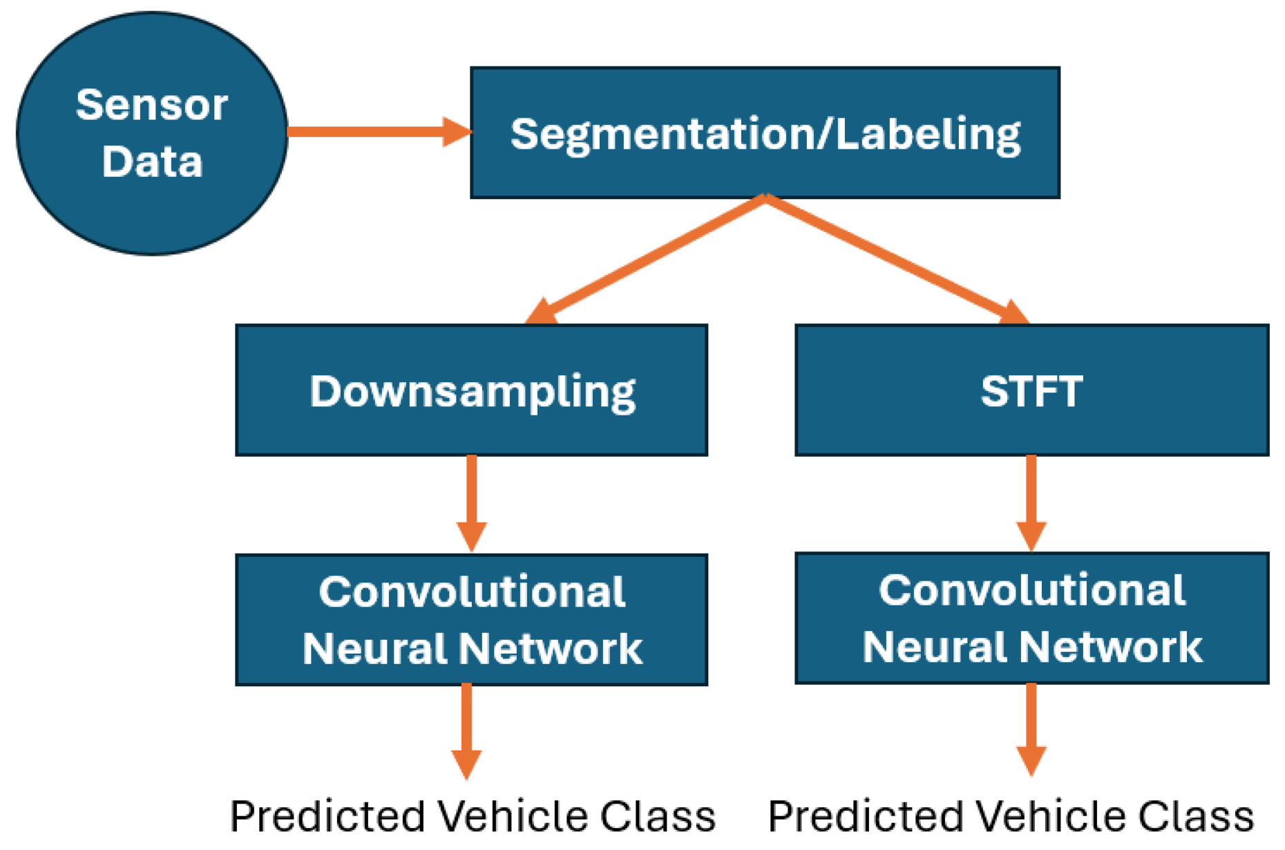
Figure 2.
Representative light vehicles used during the data collection exercise: a M923 and M934 truck.
Figure 2.
Representative light vehicles used during the data collection exercise: a M923 and M934 truck.
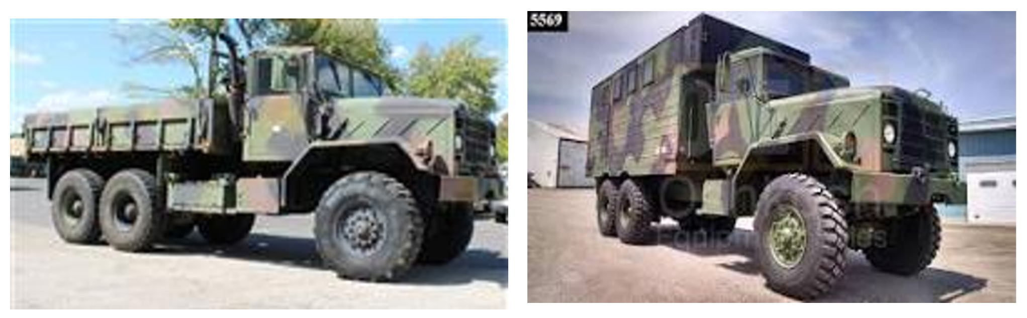
Figure 3.
Representative heavy vehicles used during the data collection exercise. These vehicles are comparable to 500-ton mobile cranes.
Figure 3.
Representative heavy vehicles used during the data collection exercise. These vehicles are comparable to 500-ton mobile cranes.
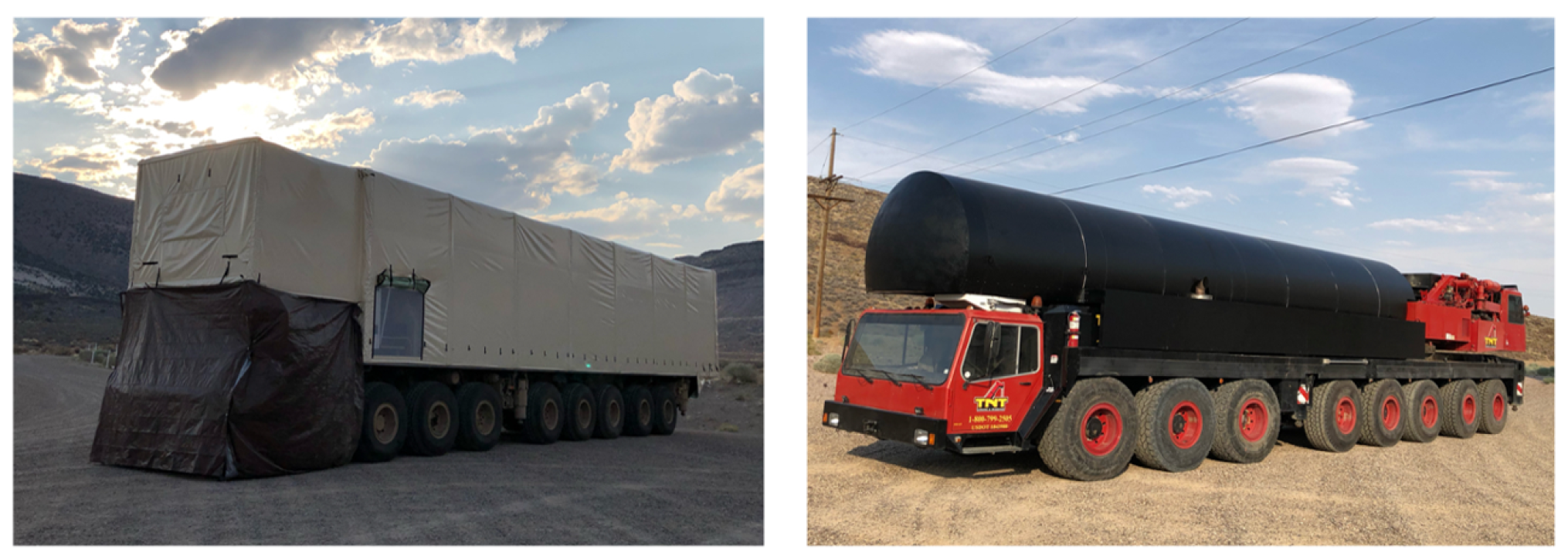
Figure 4.
Day One Sensor Layout. Four sensor units were deployed at varying distances from the road (50 and 75 meters). Diagram not to scale.
Figure 4.
Day One Sensor Layout. Four sensor units were deployed at varying distances from the road (50 and 75 meters). Diagram not to scale.
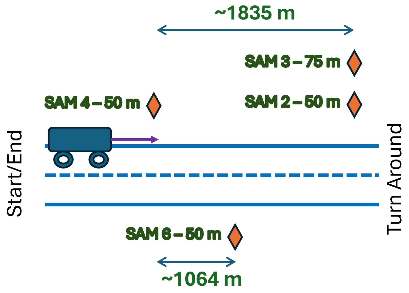
Figure 5.
Day Two Sensor Layout. Five sensor units were deployed at varying distances from the road (25, 50, 100, and 125 meters). Diagram not to scale.
Figure 5.
Day Two Sensor Layout. Five sensor units were deployed at varying distances from the road (25, 50, 100, and 125 meters). Diagram not to scale.
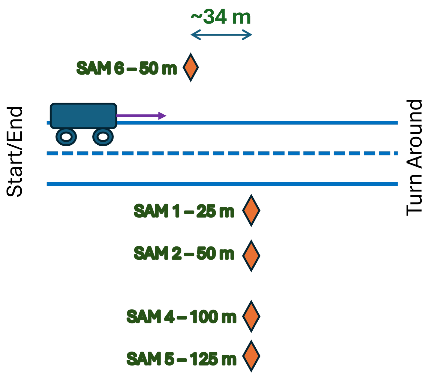
Figure 6.
Windows produced by the triggering algorithm. The black outline is the 1s average aggregated result. Each window begins with a green line and terminates with a purple line. The red lines correspond to intervals that were not associated with vehicle passes in the available GPS data and are considered false positives.
Figure 6.
Windows produced by the triggering algorithm. The black outline is the 1s average aggregated result. Each window begins with a green line and terminates with a purple line. The red lines correspond to intervals that were not associated with vehicle passes in the available GPS data and are considered false positives.
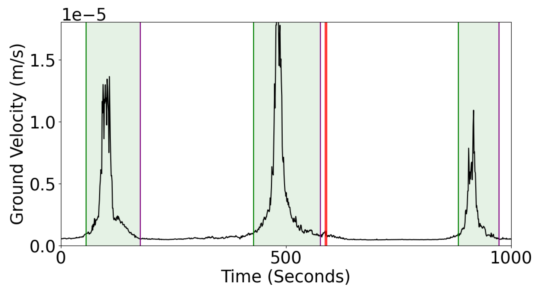
Figure 7.
Residuals for Fusion STFT-based Model and Temporally Separated Data. Residuals are provided based on vehicle class. Blue markers indicate correct classifications, while red markers denote incorrect ones. Light vehicles (a) can be further categorized into M923 and M934 models shown in Figure 2. Similarly, heavy vehicles (b) can be divided into “Test Article 1 (TA1)" and “Test Article 2 (TA2)” types, as illustrated in Figure 3. Each row in the figure represents an individual vehicle pass. The density of data points is a result of scaling the length of each pass based on the triggering algorithm.
Figure 7.
Residuals for Fusion STFT-based Model and Temporally Separated Data. Residuals are provided based on vehicle class. Blue markers indicate correct classifications, while red markers denote incorrect ones. Light vehicles (a) can be further categorized into M923 and M934 models shown in Figure 2. Similarly, heavy vehicles (b) can be divided into “Test Article 1 (TA1)" and “Test Article 2 (TA2)” types, as illustrated in Figure 3. Each row in the figure represents an individual vehicle pass. The density of data points is a result of scaling the length of each pass based on the triggering algorithm.
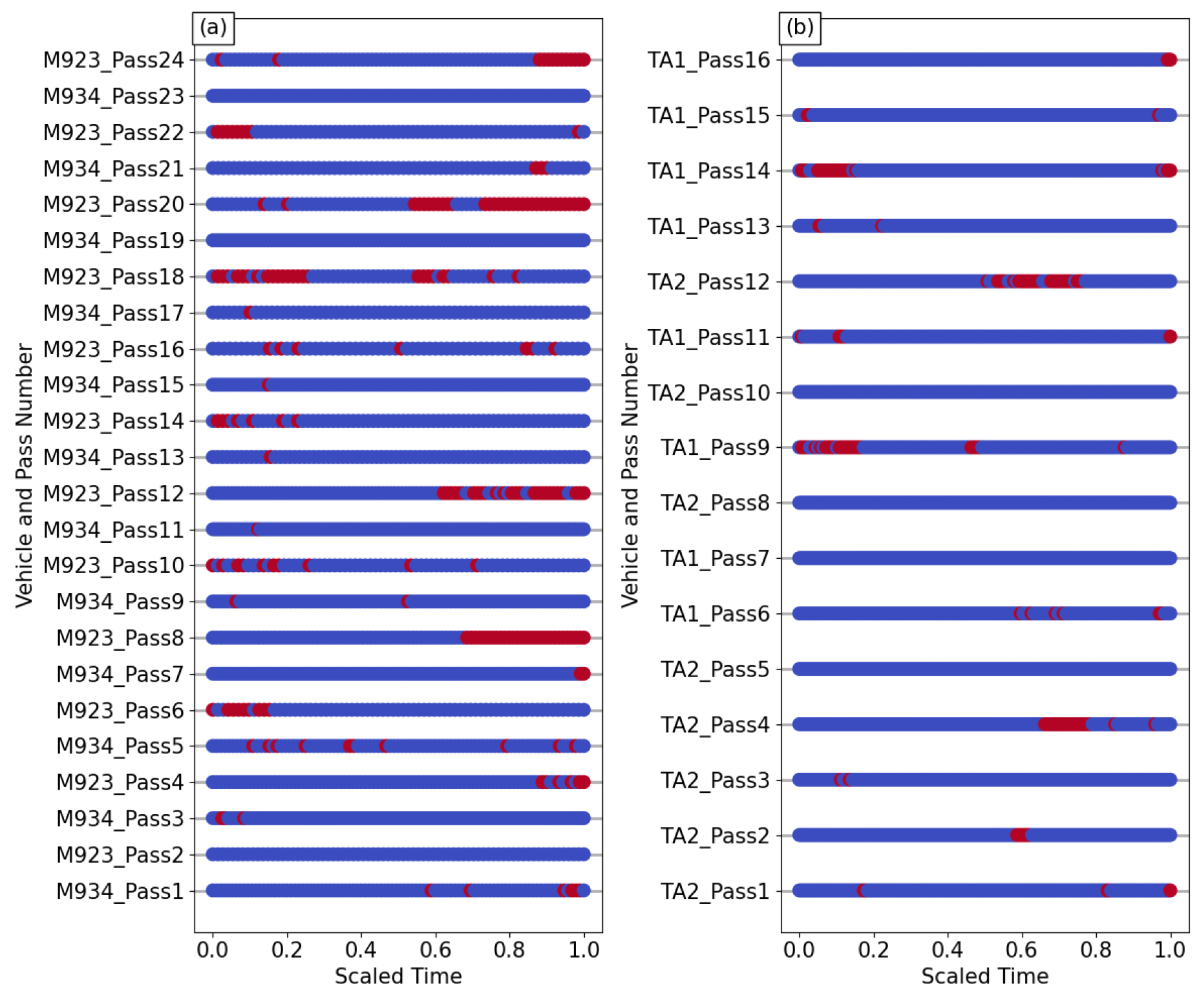
Figure 8.
Forward and Reverse Pass Residuals for Fusion STFT-based Model and Temporally Separated Data. Blue markers indicate correct classifications, while red markers denote incorrect ones. Residuals are provided for the light vehicle passes, emphasizing the direction of travel. Forward passes (a) and reverse passes (b) illustrate the error patterns as the vehicle approaches and leaves the sensor, respectively.
Figure 8.
Forward and Reverse Pass Residuals for Fusion STFT-based Model and Temporally Separated Data. Blue markers indicate correct classifications, while red markers denote incorrect ones. Residuals are provided for the light vehicle passes, emphasizing the direction of travel. Forward passes (a) and reverse passes (b) illustrate the error patterns as the vehicle approaches and leaves the sensor, respectively.
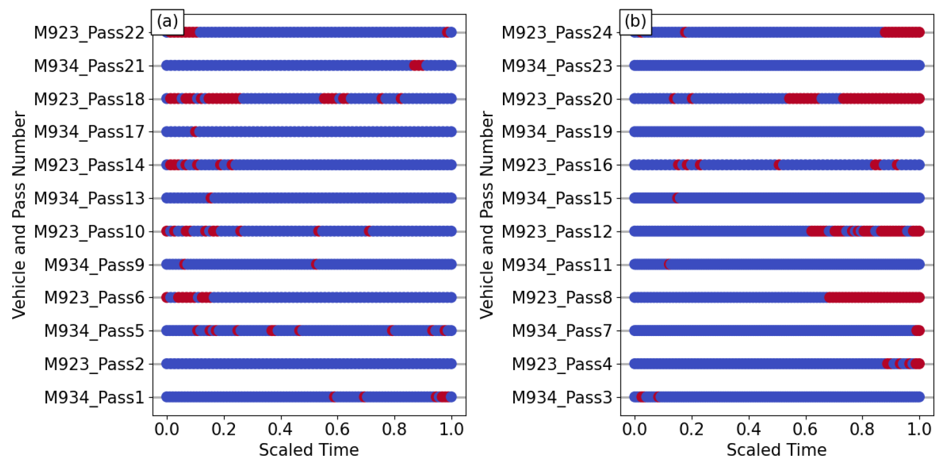
Figure 9.
Relevance Heatmap for Fusion STFT Model - Heavy Class. The top heatmap (a) corresponds to the acoustic modality. The middle heatmap (b) corresponds to the seismic modality, and bottom heatmap (c) corresponds to the magnetic modality.
Figure 9.
Relevance Heatmap for Fusion STFT Model - Heavy Class. The top heatmap (a) corresponds to the acoustic modality. The middle heatmap (b) corresponds to the seismic modality, and bottom heatmap (c) corresponds to the magnetic modality.
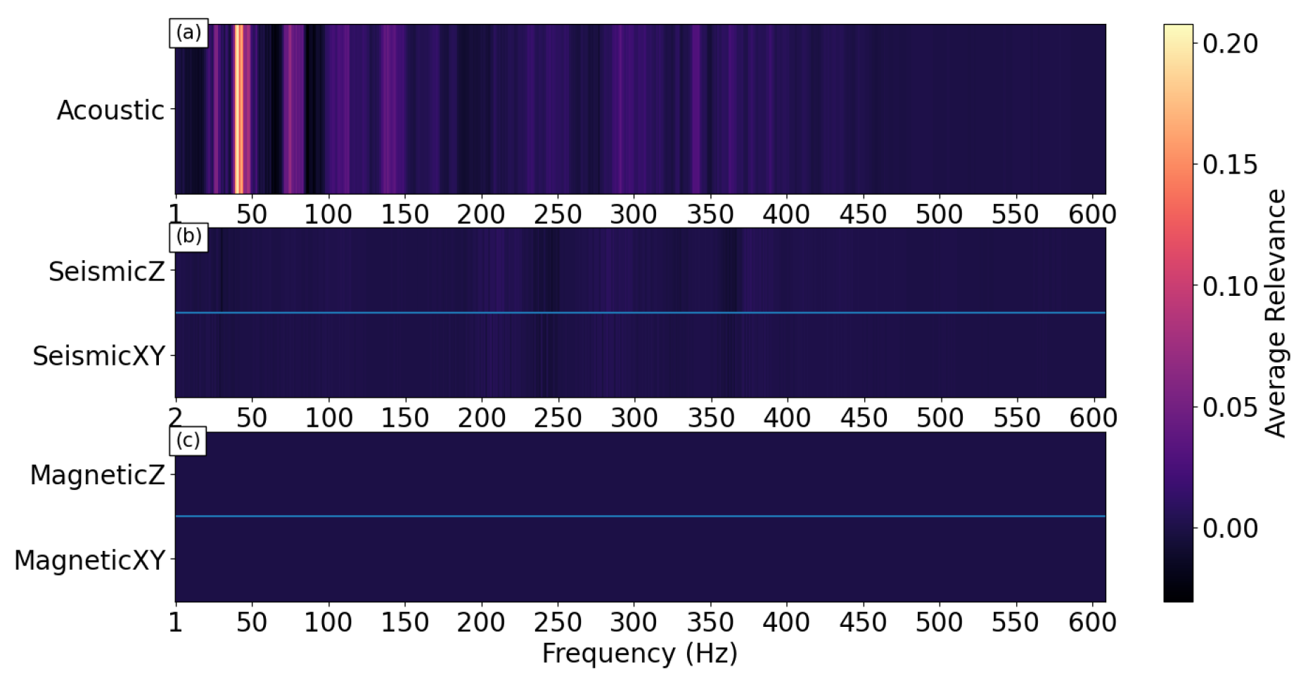
Figure 10.
Relevance Heatmap for Fusion STFT Model - Light Class. The top heatmap (a) corresponds to the acoustic modality. The middle heatmap (b) corresponds to the seismic modality, and bottom heatmap (c) corresponds to the magnetic modality.
Figure 10.
Relevance Heatmap for Fusion STFT Model - Light Class. The top heatmap (a) corresponds to the acoustic modality. The middle heatmap (b) corresponds to the seismic modality, and bottom heatmap (c) corresponds to the magnetic modality.
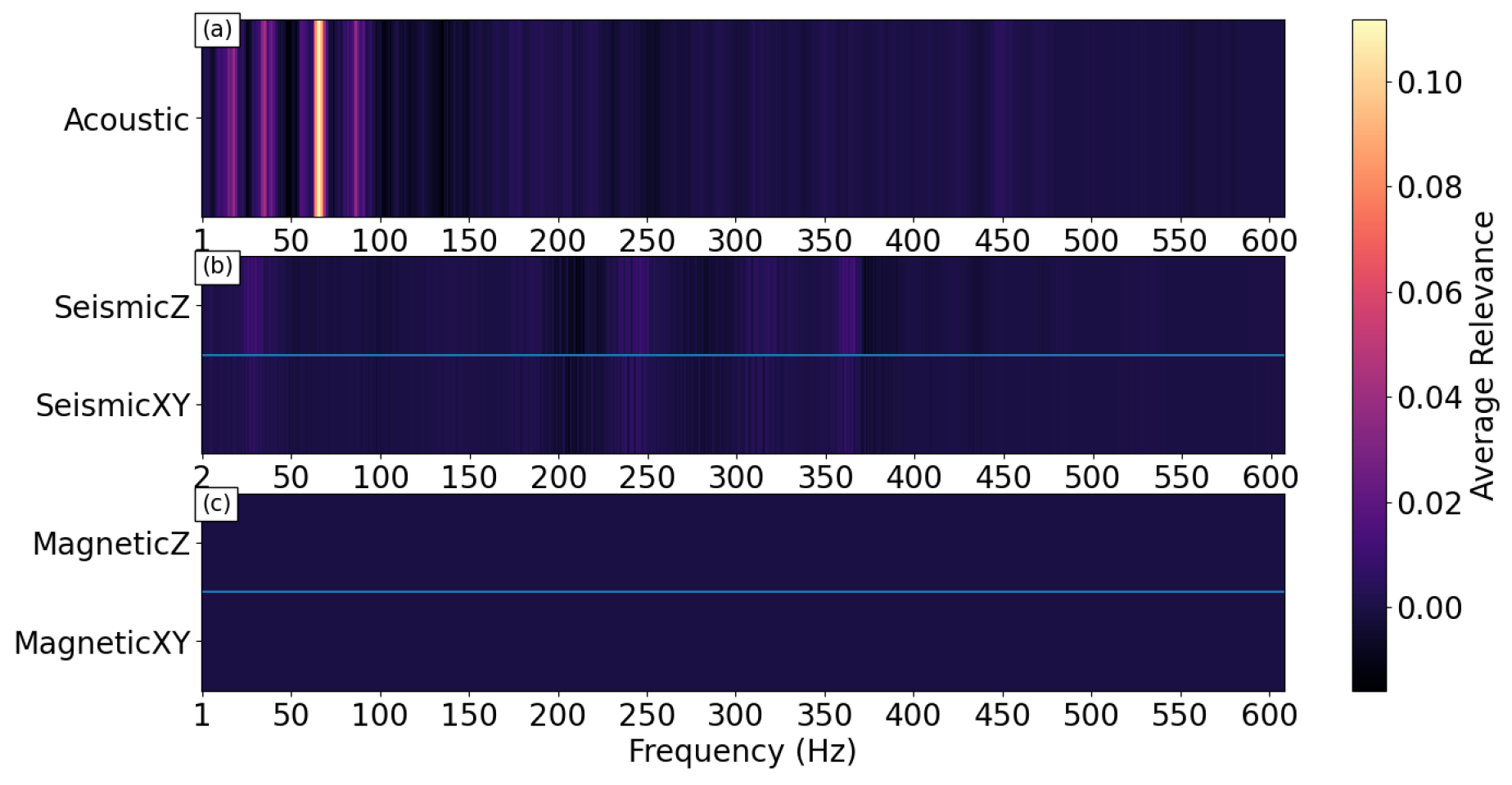
Table 1.
Number of Vehicle Passes by Day, Class, and Speed.
| Day | Vehicle Class | 24 km/h | 40 km/h | 72 km/h |
|---|---|---|---|---|
| Day 1 | Light | 12 | 12 | – |
| Heavy | 8 | 8 | – | |
| Day 2 | Light | 12 | 4 | 8 |
| Heavy | 10 | 4 | – |
Table 2.
STFT Parameter Settings.
| Parameter | Value |
|---|---|
| fs (Hz) | 8533 |
| window | “hann" |
| nperseg (samples) | 8533 |
| noverlap (samples) | 0 |
| nfft (samples) | default (nperseg) |
| detrend | “linear" |
| boundary | “None" |
| padded | “None" |
| scaling | “spectrum" |
Table 3.
Bessel Filter Parameter Settings.
| Parameter | Value |
|---|---|
| order (N) | 8 |
| (Hz) | 609 |
| btype | “lowpass" |
| norm | “mag" |
| fs (Hz) | 8533 |
Table 4.
Sensor assignments for Spatial and Temporal Partitioning approaches.
| Dataset | Spatial Partitioning (Day and Distance) | Temporal Partitioning (Day and Sensor) |
|---|---|---|
| Training | Day 1: SAM 2 (50 m), SAM 4 (50 m), SAM 6 (50 m); Day 2: SAM 1 (25 m), SAM 2 (50 m), SAM 5 (125 m), SAM 6 (50 m) | Day 2: SAM 1, SAM 2, SAM 4, SAM 5, SAM 6 |
| Validation | Day 1: SAM 3 (75 m) | Day 1: SAM 2, SAM 3 |
| Test | Day 2: SAM 4 (100 m) | Day 1: SAM 4 |
Table 5.
Considered Hyperparameter Values for CNNs.
| Hyperparameter | Possible Values |
|---|---|
| Initial weights | he_normal |
| Regularization | L2, |
| Kernel size (per layer) | |
| Stride (per layer) | |
| Number of filters | |
| Dropout rate | |
| Epochs | 500 |
| Early stopping patience | 50 |
| Optimizer | Adam (learning rate ) |
| Batch size | 128 |
Table 6.
Classification Performance under Spatially and Temporally Partitioned Test Sets.
| Partitioning | Preprocessing / Features | Balanced Accuracy (%) | Precision | Recall | MCC |
|---|---|---|---|---|---|
| Spatial | STFT - Acoustic | 0.99 | 0.99 | 0.99 | 0.98 |
| Time Series - Acoustic | 0.96 | 0.96 | 0.98 | 0.93 | |
| Temporal | STFT - Acoustic | 0.92 | 0.91 | 0.94 | 0.84 |
| STFT - Seismic | 0.91 | 0.90 | 0.95 | 0.83 | |
| STFT - Magnetic | 0.49 | 0.52 | 0.84 | -0.04 | |
| STFT - All/Fusion | 0.93 | 0.92 | 0.95 | 0.86 | |
| Time Series - Acoustic | 0.83 | 0.85 | 0.83 | 0.66 | |
| Time Series - Seismic | 0.87 | 0.92 | 0.82 | 0.74 | |
| Time Series - Magnetic | 0.50 | 0.53 | 1.00 | 0.00 | |
| Time Series - All/Fusion | 0.90 | 0.95 | 0.85 | 0.79 |
Disclaimer/Publisher’s Note: The statements, opinions and data contained in all publications are solely those of the individual author(s) and contributor(s) and not of MDPI and/or the editor(s). MDPI and/or the editor(s) disclaim responsibility for any injury to people or property resulting from any ideas, methods, instructions or products referred to in the content. |
© 2026 by the authors. Licensee MDPI, Basel, Switzerland. This article is an open access article distributed under the terms and conditions of the Creative Commons Attribution (CC BY) license.
Copyright: This open access article is published under a Creative Commons CC BY 4.0 license, which permit the free download, distribution, and reuse, provided that the author and preprint are cited in any reuse.