

Submitted:
15 August 2026
Posted:
17 August 2026
You are already at the latest version
Abstract
Europe measures the innovative performance of its regions largely by counting patents, and allocates public resources accordingly. This paper asks what regional patenting actually reflects, drawing on Regional Innovation Scoreboard data for 245 European regions observed annually between 2016 and 2023. Three candidate drivers are considered: the research effort of firms, the intensity of formal collaboration between the research base and industry, and the propensity to protect intangible assets through trademarks. Business research effort emerges as the dominant correlate throughout, science–industry collaboration as a weaker but consistent one, and trademark activity as a positive one, suggesting that firms which protect brands are not forgoing patents but exercising a single appropriation capability across several instruments. Two findings carry implications beyond measurement. Regional innovative capacity proves remarkably immobile: differences between regions account for roughly 95 per cent of the variation in the data, and differences within a region over the eight years for the remainder, so the short-run movements on which policy evaluation typically relies carry very little information, and the returns to innovation investment should be sought over horizons far longer than a programming cycle. And when the 245 regions are grouped into four innovation profiles rather than treated as a single population, the relationship that holds on average holds almost nowhere in particular: it is strong among leading and lagging regions, statistically absent in the largest group, and displaced by brand-led appropriation in a fourth group of 27 regions whose innovation is real but largely non-technological. Uniform innovation policy prescriptions and uniform managerial benchmarks are correspondingly difficult to justify.
Keywords:
regional innovation
; panel data econometrics
; patent applications
; cluster analysis
; cross-validation design
1. Introduction
Europe is worried about falling behind. The concern is no longer confined to specialist committees: it has become the organising theme of the continent's economic policy debate, and it has a simple empirical anchor. Whichever indicator one consults, the United States and China are pulling away. American firms spend a far larger share of national income on research; Chinese applicants have overtaken everyone in the international patent system and are consolidating their lead; and the technologies that will define the next decades are being assembled in laboratories and firms located, for the most part, elsewhere. Europe still produces excellent science. What it appears to be losing is the capacity to convert that science into protected, commercially deployed technology at the scale its competitors manage.
This paper does not add another lament to that literature. It asks a question that comes logically before it. Europe's response to the competitive challenge is designed and delivered at the regional scale — through cohesion funds, smart specialisation strategies, regional innovation ecosystems — and the evidence base for those instruments is a scoreboard that ranks regions largely by how much they patent. Before asking how Europe can close the gap, it is worth establishing what that measurement actually captures. Does regional patenting reflect the research effort of firms, the density of the links between science and industry, the sheer capacity of a territory to protect what it invents? Does it capture the same thing everywhere, in a Bavarian engineering district and in a Mediterranean region of design-led manufacturing? And does it move enough, over the horizon on which policy is evaluated, for anyone to observe whether an intervention worked?
These questions are the subject of the paper, which studies patent applications filed under the Patent Cooperation Treaty across the European regions over eight recent years, together with three characteristics that theory and practice suggest should account for them: the research effort of firms, the intensity of formal collaboration between the research base and industry, and the propensity to protect intangible assets through trademarks rather than patents.
Four gaps in the existing literature motivate this design. The first is circularity. A considerable body of applied work on European scoreboard data regresses a composite innovation index, or a classification of regions derived from it, on indicators that are themselves ingredients of that index. Such exercises recover the weights used to build the composite rather than any economic relationship, and they report a fit that is an artefact of arithmetic. Our specification is constructed so that the dependent variable enters none of the explanatory variables and none of them enters it. This is not a technical refinement; it is the condition under which the estimates say anything at all.
The second gap concerns time. The standard tool for panels of regions removes what is constant within each territory and identifies effects from what changes year to year. Almost nobody reports how much of the variation in these data is of that kind. We do, and the answer reframes the entire exercise: regional innovation systems turn out to be remarkably immobile. Regions differ from one another enormously and from their own recent past very little. The estimator that formal specification testing selects is therefore applied to a thin residual of the data, part of which reflects statistical interpolation rather than genuine movement. Rather than resolve the tension by deferring to a test statistic, we report both dimensions and treat the distance between them as a finding about how innovation systems actually behave.
The third gap concerns heterogeneity. Regional innovation systems are habitually described as qualitatively distinct — entrepreneurial discovery, place-based policy and specialisation are all premised on that distinctness — and then modelled as a single population governed by common parameters. We break that assumption open. Grouping the regions by their innovation profile, using a partition validated for stability rather than merely for fit, and re-estimating the same relationship within each group, we find that the association which holds on average holds almost nowhere in particular. It is strong at the top of the distribution and at the bottom, and it dissolves entirely in the large middle where most European regions live. The aggregate elasticity, the number that would be quoted in a policy brief, describes no actual group of regions.
The fourth gap concerns what patents leave out. A patent records an invention judged worth protecting; it says nothing about regions whose firms innovate in design, brand, service or process and protect the result by other means. Our taxonomy isolates precisely such a group — territories whose trademark activity far outstrips their patenting, drawn from every tier of the official ranking, including several classified as innovation leaders. A one-dimensional league table cannot represent them, and a policy that reads their position from that table will misdiagnose them as laggards.
The originality of the paper lies less in any single technique than in the decision to submit one body of data to three logics of analysis and to take their disagreements seriously. Estimation identifies associations; taxonomy asks whether those associations are shared; predictive validation reveals how much apparent explanatory success rests on knowing which region one is looking at rather than on any transferable structure. Each method has a blind spot that the other two illuminate, and it is in the friction between them that the substantive findings emerge.
The implications return to where we began. If regional innovative capacity is close to fixed over the span of a programming cycle, the returns to innovation investment must be sought over horizons far longer than those on which European instruments are currently assessed, and short-run movements in scoreboard positions are close to noise. If the determinants of patenting operate with different force in different types of region, uniform prescriptions will be miscalibrated for most of them. And if formal appropriation takes several forms, a strategy that measures success in patents alone will misread the very regions whose comparative advantage lies elsewhere. In a competition being run against the United States and China, the cost of measuring the wrong thing is not academic: it is the misdirection of the resources with which Europe intends to compete.
The remainder of the paper proceeds as follows. Section 2 reviews the literature and locates the gaps the design addresses. Section 3 describes the data and the three methods. Section 4 reports the panel econometric analysis, whose variance decomposition governs everything that follows. Section 5 partitions the regions into four profiles and re-estimates the specification within each. Section 6 tests those results out of sample under three validation designs. Section 7 discusses the findings, Section 8 draws the policy implications and Section 9 states the limitations. Section 10 concludes. Appendix A compares the taxonomy with the official Scoreboard classification; Appendix B documents the variables and reports the cluster assignment of all 245 units.
2. Literature Review
Regional patenting has been studied for two decades through a single device. The knowledge production function, transposed from the firm to the territory, treats research expenditure and human capital as inputs and patents as the observable output, and asks how much of a region's inventive performance is generated locally and how much arrives from elsewhere. The European template was set by Fritsch and Franke (2004), Moreno et al. (2005), Greunz (2005), Rondé and Hussler (2005) and Buesa et al. (2006), and extended by Buesa et al. (2010), Gumbau-Albert and Maudos (2009), Patuelli et al. (2010), Pinto and Rodrigues (2010) and Ortega-Argilés and Moreno (2009). Later work retains the structure while varying the inputs: creative employment in Antonietti (2015), foreign direct investment in Masso et al. (2013) and Ascani and Gagliardi (2015), institutional quality in Barra and Ruggiero (2022), relatedness in Martynovich and Taalbi (2023), firm-level foundations in Aronica et al. (2022) and Broekel and Brenner (2011), science parks in Gkypali et al. (2016), environmental performance in Ghisetti and Quatraro (2013), medical technology in Vadia and Blankart (2021), agglomeration in Ó hUallacháin and Douma (2021) and Lu and Liu (2025), external R&D in Brossard and Moussa (2016), high-technology services in Rodriguez (2014), regional strategy in Ott and Rondé (2019), and enterprise policy in Roper (2010) and Chan et al. (2011). Our estimates agree with this accumulated consensus in sign and in ranking: business R&D expenditure dominates in every specification, science–industry collaboration is positive but weaker, and no coefficient reverses sign across four estimators. To that extent the paper confirms the field rather than contesting it.
The agreement, however, holds in one dimension only, and this is where our results depart from the field's habits. Panels are used by Autant-Bernard and Lesage (2011), Parent (2012), Miguélez and Moreno (2013b, 2013c, 2015), Crescenzi and Rodríguez-Pose (2013), Wang et al. (2016), Qin and Du (2019), Antonelli and Colombelli (2017), Sanso-Navarro and Vera-Cabello (2018), Li et al. (2024), Tang et al. (2026), de Matos et al. (2021) and Ferreira et al. (2025), yet the distinction between variation across regions and variation within them over time is nowhere made an object of analysis, and no study reports how much of its identifying variation is temporal. Our decomposition shows why the omission matters. Differences between regions absorb the overwhelming majority of the variance of every variable in the specification, and movement within a region over eight years accounts for a small remainder, part of it interpolated from national sources rather than genuinely observed. The within transformation is therefore applied to a residual that is both thin and partly artificial, and the attenuation it produces is systematic, largest for the variable carrying the least genuine temporal movement. The assumption that a panel estimator improves on a cross-section does not hold automatically here: it depends on a variance structure that no study in this literature reports.
The largest strand concerns spillovers and proximity. Parent and Riou (2005), Del Barrio-Castro and García-Quevedo (2005), Hauser et al. (2007), Gallie (2009), Usai (2011), Grimpe and Patuelli (2011), Marrocu et al. (2013), Paci et al. (2014), Maggioni et al. (2014, 2017), Kalapouti and Varsakelis (2015), Caragliu and Nijkamp (2016), Puškárová and Piribauer (2016), Kijek and Kijek (2019), Rojas et al. (2018), Proença and Glórias (2021), Chen et al. (2022), Kekezi et al. (2022) and Kaneva et al. (2024) estimate how much inventive output derives from elsewhere, decomposing proximity into geographical, technological, social, institutional and cognitive dimensions. Networks and labour mobility carry the same logic in Miguélez et al. (2011), Miguélez and Moreno (2013a, 2013c, 2018), Cho et al. (2010), de Dominicis et al. (2013), Gonçalves et al. (2020), Costa et al. (2023), Audretsch and Belitski (2020) and Zhang et al. (2024). University–industry transmission forms a literature of its own in Drucker and Goldstein (2007), Gråsjö (2008), Rothaermel and Ku (2008), Ponds et al. (2010), Fritsch and Slavtchev (2011), Liu (2013), Fukugawa (2016, 2017), Akhvlediani and Cieślik (2017), Samandar Ali Eshtehardi et al. (2017), Barra and Zotti (2018), Chatterjee et al. (2019), De Castro Araújo and Garcia (2019), Zemtsov et al. (2016), de Castro Peixoto et al. (2022) and Ali (2024).
Within this strand sits the closest antecedent of our predictive result. Tappeiner et al. (2008) ask whether the spatial autocorrelation of European patenting is evidence of spillovers or merely a reflection of where the inputs are located, and conclude the latter. Guastella and van Oort (2015) add that omitting spatial heterogeneity inflates estimated research spillovers, and Neves and Sequeira (2018), in a meta-regression, find spillover estimates systematically lower when regional data are used and when the knowledge pool is not proxied by patents. Our grouped cross-validation reproduces this scepticism with different instruments. Once folds are constrained so that no region appears on both sides of the split, flexible algorithms lose a substantial part of their apparent accuracy, and the nearest-neighbour estimator, which most directly memorises regional levels, falls below both linear models. That a critique available to the field for nearly two decades has not been carried into the growing use of algorithmic methods on regional innovation data is itself a finding about the literature: none of the work reviewed here evaluates a model out of sample, and none reports a validation design that respects the panel structure of the data.
A second strand replaces the production function with an efficiency frontier, asking not how much a region invents but how well it converts inputs into inventions. Li (2009), Niebuhr (2010), Hudec and Prochádzková (2015), Perret (2019), Khorshid et al. (2020), Yan and Sun (2022), He et al. (2022), Popodko et al. (2019), Hussinger and Palladini (2024) and Ljungwall et al. (2022) pursue this route. It comes nearest to acknowledging that regions differ qualitatively, but it expresses the difference as distance from a common frontier, which presupposes that every region is attempting the same conversion. Our fourth profile shows that some are not.
Parameter heterogeneity is treated explicitly by a minority. Charlot et al. (2015) relax linearity, additivity and homogeneity semiparametrically, distinguishing developed from lagging regions; Kang and Dall'erba (2016a, 2016b) apply geographically weighted regression to US counties; Autant-Bernard and LeSage (2019) estimate region-specific functions for French NUTS-3 units; and Calegari et al. (2017), Mascarini et al. (2023), Limonov and Nesena (2020), Ozgen (2021), Lee and Sohn (2019) and Zheng et al. (2024) allow effects to vary with territorial or demographic characteristics. Our rejection of common slopes is consistent with this position. The difference lies in how the heterogeneity is organised, and it changes the conclusion. These studies let parameters vary over space or split the sample on an a priori development criterion; we let the data define profiles on the dimensions of the specification itself, validate the partition for bootstrap stability rather than for fit, and re-estimate within groups. Two results follow that a geographical or developed-versus-lagging cut cannot produce. The relationship breaks down not at the periphery but in the middle, where explanatory power is indistinguishable from zero and where a developed–lagging dichotomy averages precisely across the failure. And one of the profiles is not a rung on a ladder at all but a distinct appropriation regime, cutting across every tier of the official European classification.
That last result addresses the deepest silence in this literature. The identification of innovative output with patenting is near-universal, and the possibility that regions differ in the instrument through which they appropriate returns, rather than in the quantity of returns they generate, is raised nowhere: no study reviewed here observes trademarks, designs or any other formal channel alongside patents. Ó hUallacháin and Leslie (2007) come closest to a fundamental critique, arguing that the production function confounds causes with effects because regional structure determines research effort in the first place, but their remedy revises the covariates and leaves the output measure intact. Varga (2017) raises the parallel question for policy evaluation; Crescenzi and Jaax (2017) and Teslenko et al. (2021) show how poorly conclusions travel across institutional settings; Pan et al. (2020) document the dependence of measured innovation on the funding regime. The group of European regions whose trademark activity substantially exceeds their patenting, several of them officially classified as innovation leaders, is invisible to every specification in this literature because no specification measures it. The same silence surrounds the data infrastructure on which European regional policy relies: the Regional Innovation Scoreboard is almost never the object of critical scrutiny, and the circularity of regressing its composite index on its own components goes unexamined.
Our contribution is therefore not the finding that research effort drives regional patenting, which is settled, nor that parameters are heterogeneous, which is contested but established. It is the conjunction of three claims that the literature supports individually and has never assembled: that the panel dimension of European scoreboard data carries far less information than its routine use implies; that the heterogeneity which matters is organised by appropriation profile rather than by geography or development tier; and that the fact-or-artifact scepticism the field long ago applied to spatial correlation must now be applied to predictive accuracy, where it has not yet arrived. See Table 1.
3. Data and Methodology
3.1. Source and Coverage
The data are drawn from the Regional Innovation Scoreboard, the territorial companion to the European Innovation Scoreboard published by the European Commission. The Scoreboard reports, for each regional unit, a set of indicators expressed on a normalised scale on which the European Union average equals 100, so that a value of 150 identifies a region half again as intensive as the Union average on that indicator, and values are comparable across indicators measured in different underlying units — expenditure shares, counts per million inhabitants, counts per unit of GDP in purchasing power standards. The estimation sample covers 245 regional units in 31 countries, observed annually from 2016 to 2023, for a balanced panel of 1,960 region-year observations with no missing values. Coverage extends beyond the Union itself: 215 units belong to Member States and 30 to Switzerland, Norway, Serbia and the United Kingdom, which the Scoreboard tracks alongside the EU-27. The territorial grid is not uniform, and this is a property of the source rather than a choice: 193 units are NUTS2 regions, 47 are NUTS1 regions in countries where the Scoreboard reports at that level, and five are small Member States — Cyprus, Estonia, Latvia, Luxembourg and Malta — that enter as single national units because they are not regionally disaggregated. Two adjustments to the raw file deserve statement. The pseudo-region corresponding to the European Union average, present in the source, is excluded from all specifications: being an arithmetic aggregate of the remaining units, it is mechanically correlated with them and would contaminate both estimation and clustering. And one unit, NO0B (Jan Mayen and Svalbard), records zero on every indicator and carries no Scoreboard performance classification; it is retained in the descriptive tables and flagged, since its inclusion or exclusion changes no result. A third feature of the normalisation should be borne in mind when reading coefficients: the PCT scale is bounded above at 148.18, a ceiling attained by seven leading regions, so that the dependent variable is censored from above for the most inventive units.
3.2. Variables and the Non-Circularity Requirement
The dependent variable is indicator PCT patent applications: international applications filed under the Patent Cooperation Treaty, attributed to the inventor's region of residence and to the priority year, normalised by regional GDP in purchasing power standards. The econometric specification retains three explanatory indicators — business R&D expenditure (RDBUS), public–private co-publications (PPCP) and trademark applications (TM) — and the predictive exercise uses twenty, comprising every Scoreboard indicator available at regional level except the dependent variable itself.
The selection obeys one binding constraint. The Summary Innovation Index is excluded from every specification, because PCT patent applications are one of its constituent components. Eleven further Scoreboard indicators are excluded on availability grounds: they are published only at national level, carry 48 observations each rather than 1,960, and would import national variation into a regional analysis. Table A2 lists all variables, acronyms and definitions.
3.3. Panel Estimation
The baseline equation is
with regional and year effects. Year effects enter every panel specification: without them the common European decline in normalised patenting over the period is absorbed into the slopes, producing spurious associations with indicators trending in the opposite direction.
Four estimators are reported rather than one, and the reason is substantive rather than ceremonial. Pooled OLS uses all variation; the between estimator regresses regional means on regional means and uses only cross-sectional variation; the fixed-effects estimator removes regional means and uses only variation over time; random effects weights the two. The conventional protocol selects among them by specification test, and the Hausman test does reject random effects here. That guidance concerns consistency, not informativeness. Because the variance decomposition shows that within-region variation accounts for between two and five per cent of the total variance of every variable, the within estimator is applied to a thin residual, part of which reflects Scoreboard interpolation from national sources and biennial survey waves rather than genuine temporal movement. Where a regressor is measured with error, the classical attenuation is amplified by the within transformation, since differencing removes signal while leaving the error variance intact. We therefore report the between estimator as the primary specification and fixed effects as a robustness exercise, and treat the distance between the two dimensions as evidence about the data rather than as a nuisance to be resolved by a test statistic. Standard errors are clustered by region in the panel specifications and heteroskedasticity-robust (HC1) in the between regression; functional form is assessed by the Ramsey RESET test, with a logarithmic alternative estimated in the between dimension.
3.4. Taxonomy
The second method addresses a different question: whether the estimated relationship is common to all units. Regions are partitioned by K-Means with Euclidean distance, 100 random initialisations and a fixed seed, on standardised 2016–2023 averages of the four variables in the specification. Temporal aggregation follows directly from the variance structure: clustering the 1,960 region-year observations would largely group replicates of the same unit rather than distinct units. The number of groups is not selected on internal validation criteria alone, because indices such as R² and Calinski–Harabasz are monotone or nearly monotone in k and therefore reward partitions that do not reproduce in resampled data. They are supplemented by the gap statistic (Tibshirani et al., 2001) and by cluster-wise bootstrap stability measured by the Jaccard index over 200 non-parametric resamples (Hennig, 2007). The retained solution is the smallest k satisfying the gap criterion and the only one whose mean Jaccard exceeds 0.85 with no individual cluster below 0.75. The same specification is then re-estimated separately within each group, which converts the taxonomy from a descriptive device into a direct test of parameter constancy.
3.5. Predictive Validation — A Robustness Test, not a Forecasting Exercise
The third method is the one most easily misread, so its purpose should be stated plainly: the predictive exercise is not conducted to forecast regional patenting. Nothing in the paper's argument requires a forecast, and no forecast is offered. Seven algorithms — linear regression, lasso, one- and five-nearest neighbours, a single decision tree, a random forest and gradient boosting — are estimated in order to submit the econometric results to a form of scrutiny that in-sample inference cannot provide. They do so in three ways. First, out-of-sample evaluation tests whether the association identified by the between estimator survives when the model is confronted with regions it has not seen; a relationship that holds only in the sample that produced it is not a relationship. Second, the comparison of validation designs isolates the source of explanatory power. Random partitioning assigns observations to folds at random and ignores panel structure; grouped partitioning constrains all eight observations of a region to fall on the same side of the split; a temporal holdout trains on 2016–2021 and evaluates on 2022–2023. Where within-region variance is small, random partitioning allows a model to recover a test observation from a neighbouring year of the same region, and the resulting accuracy is inflated. The gap between the two designs therefore measures directly how far apparent performance rests on memorising regional levels rather than on transferable structure — the predictive counterpart of the between–within divergence documented in the econometric section, obtained by an entirely independent route. Third, permutation importance under grouped validation provides a non-parametric ranking of the twenty predictors that can be set against the coefficients of the three-variable specification: agreement is corroboration, disagreement is diagnostic. Continuous predictors are standardised within each training fold for the linear, penalised and nearest-neighbour models; importance is computed over ten permutation repetitions in each of five grouped folds.
3.6. Why the Three Methods Together
Each of the three has a blind spot that the other two illuminate. Estimation identifies associations but assumes they are common to all units and cannot test its own out-of-sample validity. Taxonomy exposes heterogeneity but says nothing about causation or generalisation. Predictive validation measures generalisation but is silent on mechanism and, applied carelessly, mistakes memorisation for understanding. Deployed together on a single body of data, their disagreements become informative in a way none of them is alone. See Figure 1.
Against the studies reviewed in Section 2, this combination is, to our knowledge, unattempted. That literature estimates the regional knowledge production function extensively, and a minority within it relaxes the homogeneity assumption — semiparametrically, geographically or by heterogeneous coefficients. But no study in the corpus reports the variance decomposition of its own panel; none evaluates a model out of sample or reports a validation design respecting panel structure; none observes trademarks or any appropriation instrument other than patents; and the Regional Innovation Scoreboard, on which European regional innovation policy rests, is almost never the object of critical scrutiny. The design set out here is assembled precisely at those four gaps: a non-circular specification, an explicit accounting of where the identifying variation lies, a data-defined and stability-validated partition to test parameter constancy, and a validation design built to distinguish structure from memorisation.
4. Panel Econometric Analysis of Regional Patenting
The dependent variable is PCT patent applications; the regressors are business R&D expenditure (RDBUS), public–private co-publications (PPCP) and trademark applications (TM), all Regional Innovation Scoreboard indicators on the normalised scale with the European Union average equal to 100. The dependent variable is not a component of any regressor and no regressor enters its construction, which distinguishes the specification from the practice of regressing the Summary Innovation Index on its own constituents, where coefficients converge on aggregation weights rather than on economic relationships. The estimation sample is a balanced panel of 245 regional units over eight years — 1,960 observations, no missing values — after excluding the pseudo-region corresponding to the European Union average, an arithmetic aggregate mechanically correlated with the remaining units. The territorial grid combines 193 NUTS2 units, 47 NUTS1 units and five national units. The baseline equation, with regional and year effects, is the one specified in Section 3. See Table 2.
Three of the four variables average below the Union benchmark of 100 — patenting at 70.2, business research at 76.6, trademarks at 88.8 — because the normalisation fixes the Union aggregate rather than the mean of regions, and the aggregate is dominated by a handful of large, intensive territories. Three regions in four fall below the benchmark on patenting, and the median region, at 64.1, is lower than the mean. Public–private co-publications are the exception, averaging 148.2, since the indicator is scaled per million inhabitants and rewards small research-dense units.
Every variable ranges from an exact zero to a maximum attained repeatedly rather than uniquely: 148.18 for patenting, reached in 103 observations by eighteen regions; 157.40 for business R&D, reached by ten; 245.91 for trademarks, reached by eight. These are ceilings imposed by the Scoreboard’s normalisation, not empirical ties, which means the dependent variable is censored from above precisely for the most inventive units — relevant when reading coefficients estimated in levels.
The higher moments are unremarkable, and that is itself notable. Skewness runs from 0.18 to 0.82, kurtosis from 2.14 to 3.26, with patenting mildly platykurtic. Raw patent counts are among the most skewed quantities in applied economics and normally demand count models; here the normalisation and the ceiling have compressed the tail before the data reach the analyst. Linear estimation is thereby licensed, but the convenience is manufactured rather than found.
The final three columns carry the section’s governing fact. The between standard deviation is nearly indistinguishable from the total in every case — 39.27 against 39.60 for patenting, 36.33 against 36.70 for business R&D — while the within standard deviation is a small fraction of it. Variation over time within a region accounts for 2.03 per cent of the total variance of patenting, 2.34 per cent for business R&D, 4.59 per cent for co-publications and 5.10 per cent for trademarks. A typical region moves fewer than six points on a 148-point scale across eight years, while the distance between regions spans that scale almost entirely. The fixed-effects transformation therefore discards roughly ninety-five per cent of the available information, and what remains is not wholly genuine: several Scoreboard indicators are interpolated from national sources or biennial survey waves, so part of the residual temporal variation is an artefact of compilation. Every result reported below should be read against this decomposition. See Table 3.
Table 2 establishes an ordering that survives every estimator reported later. Business R&D expenditure is the regressor most strongly associated with patenting, at 0.770; public–private co-publications follow at 0.654; trademark applications are weakest at 0.448. That the ranking of simple correlations reproduces the ranking of estimated coefficients is reassuring rather than trivial: it indicates that the multivariate results are not driven by suppression or by a particular conditioning set, and that the specification is describing a structure already visible in the raw pairwise associations.
The off-diagonal correlations among regressors are more informative than they first appear. Business R&D and co-publications correlate at 0.619, which is unsurprising — both measure formalised research activity, and regions with intensive corporate laboratories are also regions whose firms co-author with universities. Trademarks behave differently. Their correlation with co-publications is moderate (0.512) but with business R&D only 0.360, the weakest pair in the matrix. Trademark activity therefore carries information substantially independent of research effort. This is the first quantitative sign of the appropriation argument developed in the cluster analysis: brand-based protection is not simply a by-product of research intensity, and a territory can be active in one without being active in the other. Had trademarks correlated with R&D at 0.7 or above, the fourth cluster identified later would have been an artefact of scale rather than a distinct configuration. See Table 4.
Table 4 addresses whether these interdependencies threaten identification. They do not. All variance inflation factors lie below 2.5, comfortably under the conventional threshold of 10 and under the stricter threshold of 5 favoured in applied work. The highest, on co-publications, is 1.980, implying that collinearity inflates the variance of that coefficient by less than a factor of two. The diagnostic is reported in both dimensions deliberately, and the near-identity of the two columns matters: 1.661 against 1.627 for business R&D, 1.980 against 1.920 for co-publications. The correlation structure among regressors is essentially the same whether computed on regional means or on pooled observations, which rules out one candidate explanation for the between–within divergence documented in Table 5 and Table 6. That divergence cannot be attributed to collinearity behaving differently across dimensions, because it does not.
One earlier specification is worth recording. Including international scientific co-publications alongside public–private co-publications and top-decile cited publications produced variance inflation factors of 8.3 and 10.1 in the between dimension — three overlapping measures of the same underlying construct, scientific connectivity. Only one such measure is retained here. Finally, a caveat on what this table cannot show: variance inflation factors speak to the precision of coefficients, not to their consistency. Low collinearity offers no protection against the measurement-error attenuation that Table 6 documents.
Two features of this table deserve equal attention: what is stable across the four columns, and what is not. What is stable is the substance. All three coefficients are positive under every estimator, none reverses sign, and the ordering RDBUS > PPCP > TM holds throughout. Business R&D expenditure is significant at the one per cent level in all four specifications. Read on the between estimator, a region positioned ten points higher on the business research scale records roughly 6.4 points more patenting, a region ten points higher on co-publications about 1.3 points more, and a region ten points higher on trademarks about 0.9 points more. The positive trademark coefficient is substantively important: it indicates that technological and non-technological appropriation are complementary rather than substitutive at the regional level. Firms that protect brands are not forgoing patents; formal appropriation appears to be a single organisational capability exercised across instruments.
What is not stable is the magnitude, and the pattern of instability is systematic. Pooled OLS and the between estimator are nearly identical — 0.6242 against 0.6352 on business R&D, 0.1343 against 0.1332 on co-publications. When ninety-five per cent of the variance is cross-sectional, pooled OLS is arithmetically almost the between estimator with extra observations. The fixed-effects column is a different object altogether: 0.1028 on business R&D, roughly one sixth of the between value, with co-publications and trademarks falling to 0.0318 and 0.0306 and both dropping to ten per cent significance. Random effects lands between the two at 0.2803, as its construction requires.
The fit statistics complete the picture. The between regression explains 68.7 per cent of the cross-sectional variation in regional patenting with three variables on 245 units; the within R² is 0.0794. These numbers are not competing measures of the same quantity — they refer to different variation — but their ratio conveys where the explanatory content lies.
The conventional response is to invoke the Hausman test, which rejects random effects and directs the analysis to fixed effects. That guidance concerns consistency, not informativeness. Given the variance structure, the within estimator is applied to a thin and partly interpolated residual, and Table 6 shows that its attenuation is ordered exactly as measurement-error theory predicts. We therefore report the between estimator as the primary specification and fixed effects as a robustness exercise, treating the gap between the columns as a finding about the persistence of regional innovation systems rather than as a nuisance to be arbitrated by a specification test.
Table 6 is the diagnostic on which the paper’s methodological argument rests. Reading the last two columns together, the attenuation ratio and the within-variance share are perfectly inversely ordered across the three regressors: business R&D has the least temporal variation (2.34 per cent) and suffers the greatest attenuation (a factor of 6.18); trademarks have the most temporal variation (5.10 per cent) and suffer the least (3.02); co-publications sit between on both counts. The rank correlation is exactly minus one.
This ordering is the signature of classical measurement-error attenuation amplified by the within transformation. Differencing away regional means removes signal while leaving the error variance untouched, so the attenuation factor rises as the genuine temporal signal falls. The alternative interpretation — that the between and within coefficients estimate economically distinct short-run and long-run relationships — cannot be excluded on statistical grounds alone, but it does not predict this correspondence. That the ranking of attenuation should reproduce the ranking of temporal information content exactly, across three regressors of very different magnitude, is difficult to attribute to coincidence. See Table 7.
Table 7 quantifies the asymmetry between the two panel dimensions. The between-unit variance component, 499.35, exceeds the within-unit component, 33.75, by a factor of 14.8; the intra-class correlation is 0.9367, meaning that nearly ninety-four per cent of the residual variance is regional rather than temporal. The theta parameter governing the GLS transformation is 0.9085, close enough to unity that random effects is approximating the within estimator — which is precisely why its coefficients sit closer to fixed effects than to between in Table 4, and why the choice between them is less consequential than the choice between either and the cross-sectional dimension.
The final block is the most damaging to a naive reading of the within results. A specification containing year dummies alone attains a within R² of 0.0611; adding the three regressors raises it to 0.0794. The net contribution of business R&D, co-publications and trademarks to the within-dimension fit is therefore 0.0182 — under two percentage points. More than three quarters of the apparent within explanatory power is the common European time profile documented in Table 8, not the explanatory variables. The overall R² of the fixed-effects specification, 0.2900, is respectable only because it incorporates the regional effects themselves, which are estimated parameters rather than substantive findings.
Every coefficient is negative, every one is significant, and the sequence increases monotonically in absolute value from −1.38 in 2017 to −7.39 in 2023. Relative to 2016, the average European region lost 7.4 points of normalised patenting over seven years. Two comparisons give that figure meaning. Against the sample mean of 70.24 it represents a decline of roughly ten per cent. Against the within standard deviation of 5.65 it represents 1.31 standard deviations — that is, the common European time profile moves regional patenting by more than a typical region moves relative to its own average. This single observation explains why year dummies alone account for 0.0611 of the 0.0794 within R² reported in Table 7: in the temporal dimension, the dominant signal is not regional differentiation but a shared European trajectory.
The profile of the decline is worth reading closely. It is steady but not uniform. The step from 2016 to 2018 is the steepest of the early period (−1.38 to −2.97), after which the series flattens markedly: 2019 to 2022 adds barely 1.5 points in total, and the increments narrow to −0.14 between 2021 and 2022. The final year then breaks the pattern, with the coefficient jumping from −4.65 to −7.39, an increment larger than any other in the series. Two readings are available and the data cannot arbitrate between them. The decline may be genuine, reflecting the documented weakening of European positions in international patenting relative to Asian and North American applicants. Or it may be partly compositional, arising from revisions to the Scoreboard’s normalisation base or from the incomplete maturation of the most recent priority years, since PCT applications are attributed to the priority year and the latest cohort is the least complete at the time of compilation. The standard errors themselves hint at the second possibility, rising steadily from 0.51 in 2017 to 0.91 in 2023 — the later coefficients are estimated with progressively less precision.
Whichever reading is correct, the practical implication for specification is unambiguous, and it justifies the decision to include year effects in every panel estimate. Omitting them transfers this trajectory into the slopes. In an unreported specification without year dummies, international scientific co-publications — an indicator that trends upward across the period — enter with a negative and statistically significant coefficient, which reverses sign and loses significance as soon as the time profile is controlled for. A shared downward movement in the dependent variable, if left unmodelled, manufactures spurious negative associations with any regressor trending the other way. See Table 9.
Table 9 returns a mixed verdict that the analysis follows rather than overrides. The Ramsey RESET rejects the linear functional form in the pooled specification (7.942, p = 0.0004) but does not reject it in the between dimension (1.220, p = 0.297). Since the between regression is the primary specification, the evidence on functional form is favourable precisely where it matters, and the pooled rejection is plausibly driven by the repeated within-region observations that pooling treats as independent.
The null of homoskedasticity is rejected in both dimensions — White statistics of 310.15 and 43.42 — which is expected in cross-regional data spanning territories of very different size. The response is robust and clustered covariance estimation rather than weighted least squares, since the coefficient estimates remain consistent and only the standard errors require correction. Residual normality is rejected everywhere, most sharply in the fixed-effects specification (745.47), where the within transformation concentrates the residuals around zero and the ceiling on the dependent variable truncates the upper tail. At these sample sizes non-normality affects neither consistency nor, asymptotically, inference.
The Durbin–Watson statistic of 0.2241 signals strong positive serial correlation, which is not a pathology but a restatement of Table 2: regional patenting is highly persistent, and consecutive observations of the same unit are close to identical. Clustering standard errors by region is the appropriate response and is applied throughout. Joint significance is comfortably attained in both dimensions. See Table 10.
Table 10 reports the logarithmic alternative. The elasticities are all positive and significant: doubling business R&D expenditure is associated with a 53 per cent increase in patenting, doubling co-publications with 38 per cent, doubling trademarks with 11 per cent. The fit, 0.6768, is essentially that of the linear between regression. The substantive novelty is the changed relative weight of co-publications: in levels they carry roughly one fifth of the business R&D coefficient, in logs more than two thirds of it. Proportional reasoning therefore raises the apparent importance of science–industry linkage, which is intuitive if its effect operates multiplicatively on an existing research base rather than additively.
One result must be reported plainly rather than glossed. The RESET statistic for the logarithmic specification is 16.337 with p < 0.0001: the log–log form is rejected more decisively than the linear between form, which was not rejected at all. The logarithmic specification is therefore presented as an alternative parameterisation yielding interpretable elasticities and confirming the robustness of sign and ranking — not as a better-specified model. On the criterion of functional form, the linear between regression remains the preferred specification.
5. Cluster Analysis of European Regions
The taxonomy is built on 2016–2023 averages of the four indicators retained in the econometric specification — PCT patent applications, business R&D expenditure, public–private co-publications and trademark applications — for the same 245 regional units, standardised before clustering. Temporal aggregation follows directly from the variance structure documented in Section 4: with within-region variance accounting for between two and five per cent of the total, clustering the 1,960 region-year observations would largely group repeated observations of the same unit rather than distinct units. The algorithm is K-Means with Euclidean distance, 100 random initialisations and a fixed random seed. The number of groups is not chosen on internal validation criteria alone, for reasons Table 11 makes plain, and is corroborated by resampling evidence in Table 12.
Table 11 illustrates why internal criteria cannot settle the choice on their own. Two of the seven indices are effectively predetermined. R² rises monotonically from 0.465 at k = 2 to 0.796 at k = 10, as it must: adding centroids can only reduce within-cluster dispersion, so the criterion rewards fragmentation without limit. Calinski–Harabasz falls monotonically from 211.3 to 101.9 over the same range, which in this sample amounts to an equally mechanical preference for k = 2. Read alone, the two most commonly reported indices would point in opposite directions and neither would be informative.
The remaining criteria carry more information because they are not monotone. Silhouette attains its global maximum at k = 2 (0.389), which reflects the elementary observation that a leading group and a lagging group are easy to separate, but it then falls to 0.299 at k = 3 and recovers to 0.318 at k = 4 before declining steadily thereafter. That local maximum is the first indication that the four-group solution recovers structure the three-group solution had merged. Davies–Bouldin behaves symmetrically, deteriorating from 0.988 to 1.211 between k = 2 and k = 3 and improving to 1.101 at k = 4, its best value above k = 2.
The two geometric measures are the most decisive. The Dunn index, which relates the closest distance between clusters to the widest diameter within them, reaches its maximum across the whole range at k = 4 (0.084), well above the 0.055 to 0.071 recorded at k = 2, 3 and 5 and roughly double the 0.036 to 0.037 obtained at k = 9 and 10. Minimum separation tells the same story from the other direction: 0.385 at k = 4 is the largest value in the column, and it collapses to 0.130 by k = 10, meaning that the additional groups produced by finer partitions are not separated from their neighbours in any meaningful sense. Maximum diameter, meanwhile, drops sharply from 5.94 at k = 3 to 4.60 at k = 4 — the largest single improvement in the column — and then flattens.
Taken together, four of the five non-monotone criteria identify k = 4 as the best partition above the trivial two-group split, and the two monotone criteria are uninformative by construction. This is suggestive but not sufficient. Internal criteria measure geometric properties of the partition in the sample that produced it; none of them asks whether the same partition would reappear in different data. That question is addressed in Table 12.
Table 12 replaces the question “which partition fits best?” with two harder ones: does the partition improve on what random data would produce, and does it survive resampling? The gap statistic answers the first. Gap values rise from 0.883 at k = 2 to a maximum of 1.005 at k = 5, but the raw maximum is not the decision rule. The standard criterion selects the smallest k for which Gap(k) − Gap(k+1) + s(k+1) is non-negative, and that condition first holds at k = 4 (0.0249), the values at k = 2 and k = 3 being negative. Four groups is therefore the most parsimonious partition that the gap procedure does not reject in favour of a finer one.
The bootstrap evidence is more discriminating still, and it works in the opposite direction to the internal criteria of Table 11. Stability is highest where structure is coarsest: at k = 2 the mean Jaccard is 0.959 and the least stable cluster scores 0.955, so the leading–lagging dichotomy reproduces almost perfectly in resampled data. It is, however, a partition that tells us little. At k = 3 stability remains high (0.887 mean, 0.856 minimum). At k = 4 the mean falls to 0.851 — still above the 0.85 threshold conventionally taken to indicate a highly stable solution — with a minimum of 0.732 in a single cluster, which places that group in the “uncertain” band rather than the unreliable one.
Beyond four groups the deterioration is abrupt rather than gradual. At k = 5 the mean drops to 0.752, three clusters fall below 0.75, and the least stable scores 0.685. From k = 6 onwards the solutions cease to be interpretable as structure at all: mean Jaccard between 0.498 and 0.586, minimum values between 0.322 and 0.450, and five to ten clusters below the reliability threshold in every case. A cluster with a Jaccard of 0.35 is recovered in roughly one bootstrap sample in three; it is an artefact of the particular 245 observations in hand, not a feature of European regional innovation.
The two tables therefore converge from independent directions. The four-group solution is the smallest partition satisfying the gap criterion, the only one whose mean Jaccard exceeds 0.85 with no cluster falling below 0.75, and the one that maximises the Dunn index and minimum separation in Table 11. It also preserves a smallest group of 27 units — large enough to support the within-cluster estimation reported in Table 15, whereas the smallest groups at k = 8 to k = 10, containing ten to twelve units, would not be. See Table 13.

Table 13.
Standardised cluster centroids.
| Cluster | N | % of sample | z PCT | z RDBUS | z PPCP | z TM |
|---|---|---|---|---|---|---|
| 1 — Leading | 54 | 22.0 | 1.41 | 1.20 | 1.09 | 0.76 |
| 2 — Peripheral | 80 | 32.7 | −1.02 | −0.99 | −0.94 | −0.70 |
| 3 — Intermediate | 84 | 34.3 | 0.13 | 0.24 | 0.03 | −0.34 |
| 4 — Trademark-oriented | 27 | 11.0 | −0.19 | −0.21 | 0.51 | 1.59 |
Note. Centroids expressed in standard deviations from the sample mean of the standardised variables.
Table 14.
Cluster profiles on the original scale and internal diagnostics.
| Cluster | PCT | RDBUS | PPCP | TM | Within sum of squares | Silhouette | Jaccard |
|---|---|---|---|---|---|---|---|
| 1 — Leading | 125.6 | 119.9 | 226.8 | 129.0 | 94.2 | 0.289 | 0.881 |
| 2 — Peripheral | 30.1 | 40.7 | 80.2 | 52.0 | 72.0 | 0.451 | 0.950 |
| 3 — Intermediate | 75.3 | 85.2 | 150.5 | 71.0 | 111.8 | 0.243 | 0.856 |
| 4 — Trademark-oriented | 62.6 | 69.0 | 185.2 | 172.5 | 56.1 | 0.215 | 0.751 |
Note. Levels on the RIS index scale, where the European Union average equals 100. Within sums of squares are computed on standardised data; Silhouette and Jaccard are cluster averages.
Table 15.
Parameter heterogeneity: the specification estimated separately within each cluster.
| Group | N | RDBUS | S.E. | PPCP | S.E. | TM | S.E. | R² |
|---|---|---|---|---|---|---|---|---|
| Cluster 1 — Leading | 54 | 0.394*** | (0.106) | −0.018 | (0.055) | 0.055 | (0.049) | 0.257 |
| Cluster 2 — Peripheral | 80 | 0.291*** | (0.071) | 0.087** | (0.035) | 0.074 | (0.051) | 0.415 |
| Cluster 3 — Intermediate | 84 | −0.002 | (0.127) | −0.013 | (0.052) | 0.062 | (0.087) | 0.007 |
| Cluster 4 — Trademark | 27 | 0.270 | (0.176) | 0.034 | (0.040) | 0.147 | (0.185) | 0.115 |
| Full sample | 245 | 0.635*** | (0.067) | 0.133*** | (0.033) | 0.092*** | (0.032) | 0.687 |
Note. Ordinary least squares on 2016–2023 regional averages, corresponding to the between dimension of the panel; heteroskedasticity-robust (HC1) standard errors in parentheses. *** p < 0.01; ** p < 0.05; * p < 0.10.
Table 13 shows that three of the four groups differ from one another in level while the fourth differs in shape, and the distinction matters for everything that follows. Clusters 1, 2 and 3 form a ladder. The leading group sits between 0.76 and 1.41 standard deviations above the mean on all four indicators; the peripheral group sits between 0.70 and 1.02 standard deviations below on all four; the intermediate group sits close to the mean on three of them. Within this ladder the ordering of the indicators is almost identical, and a single latent dimension — call it innovative intensity — would reproduce the three centroids with little loss. Had the analysis stopped at k = 3, this is the entire structure it would have recovered, and it would have been a rediscovery of the ranking the Scoreboard already publishes.
Cluster 4 is not on that ladder. Its centroid is slightly below the mean on patenting (−0.19) and on business research (−0.21), moderately above on co-publications (0.51), and 1.59 standard deviations above on trademarks — the largest single deviation anywhere in the table, exceeding even the leading group’s patenting centroid. The profile cannot be produced by moving a region up or down a scale of intensity, because its coordinates point in different directions on different axes. These 27 regions are not weak innovators; they are territories whose formal appropriation runs through brands rather than through patents.
Two further features deserve comment. The intermediate group, which is the largest at 84 units and 34.3 per cent of the sample, has a centroid within a quarter of a standard deviation of the mean on three indicators and −0.34 on trademarks. It is defined less by what it is than by what it is not, and this will be reflected in its internal diagnostics in Table 14 and, more consequentially, in the failure of the econometric relationship within it reported in Table 15. Meanwhile, the leading group’s weakest coordinate is trademarks (0.76), which is well above the mean but distinctly less extreme than its patenting (1.41): even at the top of the European distribution, technological and non-technological appropriation are not the same thing.
The composition of the sample is also informative. The two extreme groups account for 54.7 per cent of the units between them, leaving a broad middle of 84 regions and a small distinct group of 27. The European regional distribution, on these four indicators, is neither bimodal nor uniform: it has thick shoulders, a heavy centre, and one configuration that a one-dimensional ranking cannot represent at all. See Table 14.
Read on the original scale, the four profiles acquire economic content. The leading group records 125.6 on patenting and 226.8 on co-publications, both far above the Union benchmark, on a business research base of 119.9. The peripheral group is below the benchmark on every indicator, at 30.1 on patenting and 40.7 on business research — not a marginal shortfall but a different order of magnitude. The intermediate group is close to the benchmark on research (85.2) and co-publications (150.5, which is near the sample mean given how that indicator is scaled), but records only 71.0 on trademarks.
The fourth group is the interpretive centre of the analysis. Trademark applications average 172.5 against patent applications of 62.6 — a ratio of nearly three to one, in a sample where the corresponding ratio is close to unity in the leading group and where every other group patents more than it trademarks relative to the benchmark. Co-publications are high at 185.2 while business research is below benchmark at 69.0, a combination suggesting territories connected to the scientific system without a large corporate research base of their own. This is the configuration that a patent-based ranking necessarily reads as underperformance, and that Appendix shows to include several regions the Scoreboard itself classifies as innovation leaders.
The internal diagnostics qualify the confidence attaching to each group. The peripheral cluster is the most coherent by a wide margin: silhouette 0.451, Jaccard 0.950, and the second-lowest within sum of squares. Low-performing regions resemble one another closely, which is intuitive — there are many ways to be innovative and rather few ways to be uninnovative. The leading group is also solid (silhouette 0.289, Jaccard 0.881).
The remaining two are weaker, for opposite reasons. The intermediate group has the highest within sum of squares in the table (111.8) and a low silhouette (0.243) despite a high Jaccard (0.856): it reproduces reliably in bootstrap samples because its boundaries are stable, but it is internally dispersed and its members sit close to the boundaries with other groups. It is, in effect, the residual. The trademark-oriented group is the mirror image: the lowest within sum of squares in the table (56.1), so it is by far the most compact group in the sample, but the lowest silhouette (0.215) and the lowest Jaccard (0.751). Its members are similar to each other yet not far from the centroids of neighbouring clusters, which is exactly what one expects of a group that differs from the others in orientation rather than in magnitude. The 0.751 places it at the boundary between the stable and uncertain bands, and this is stated plainly rather than glossed: the group is the least secure of the four, and the substantive weight the paper places on it rests on its economic interpretability and on the corroborating evidence of Appendix, not on its stability score alone. See Table 15
Table 15 is the substantive core of the section. Estimated on all 245 units, the coefficient on business R&D expenditure is 0.635 and significant at the one per cent level, with an R² of 0.687. Estimated separately within the four groups, the same coefficient takes the values 0.394, 0.291, −0.002 and 0.270. The aggregate figure lies outside the range of every subgroup estimate. It is not an average of the four in any useful sense; it is a between-profile effect, generated by the fact that regions with high research intensity belong to clusters that also patent heavily, and it should not be read as the response of any actual region to a change in its research base.
The pattern across groups is orderly. Business research retains a strong and significant association in the leading group (0.394) and in the peripheral group (0.291), the two configurations at the extremes of the distribution. It disappears entirely in the intermediate group, where the point estimate is −0.002 with a standard error of 0.127 and the model explains 0.7 per cent of the variance. This is the largest of the four groups, comprising 84 regions and more than a third of the sample. In the modal European region, the relationship on which the aggregate result rests is not detectable.
Co-publications behave similarly, significant only in the peripheral group (0.087) and indistinguishable from zero elsewhere, with a point estimate that is actually negative in the leading and intermediate groups. Trademarks are never individually significant within groups, although the point estimate in the trademark-oriented cluster (0.147) is the largest of the four and roughly sixty per cent above the full-sample value — consistent with, though not evidence for, an appropriation logic specific to that group. Its standard error of 0.185 on 27 observations makes clear how little should be concluded from it.
Two caveats belong here. First, statistical power falls with sample size, and the trademark-oriented group has 27 units; the absence of significance there is weak evidence of the absence of an effect. Second, and more fundamentally, partitioning the sample restricts the range of the regressors within each group, which mechanically reduces both the estimated coefficients and R² relative to the full sample. Neither caveat accounts for the pattern observed. Restriction of range would attenuate all four subgroup coefficients towards zero roughly uniformly; it would not produce estimates of 0.394 and 0.291 in two groups and −0.002 in a third that is larger than either. Nor would it explain why the group with the most units and the widest internal dispersion — Cluster 3, which Table 14 shows to have the highest within sum of squares — is precisely the one where the relationship vanishes. The evidence supports the stronger reading: the parameters of the regional knowledge production function are not common across European regional profiles, and the aggregate elasticity so frequently quoted in policy discussion describes no group of regions in particular. See Table 16.
Table 16 asks whether the taxonomy is anything more than a map of national borders. It is not — but neither is it independent of them, and the mixture is the finding. Some national systems are internally homogeneous: all eight Romanian units and all four Serbian units fall in the peripheral cluster, twelve of thirteen Greek units do the same, and six of seven Swiss units and three of three Austrian units sit in the leading cluster. For these countries, national membership predicts cluster membership almost perfectly.
The larger and more diversified economies behave differently. Italy spans all four clusters, with a single leading region, six peripheral, nine intermediate and five trademark-oriented. Germany occupies three of the four, splitting twenty leading units against sixteen intermediate ones and two trademark-oriented. Spain likewise spans three, and so do the Netherlands, the United Kingdom, Czechia, Portugal and Norway. In these countries the internal dispersion of regional innovation profiles is comparable in magnitude to the dispersion across countries, which has a direct methodological implication: country fixed effects, a standard device in this literature, would absorb a substantial part of the variation this paper is trying to explain, and would do so unevenly — harmlessly in Romania, destructively in Italy and Germany.
The trademark-oriented cluster is the most geographically dispersed of the four. Its 27 units come from seventeen different countries, spanning Switzerland, Germany, the Netherlands, the United Kingdom and Belgium at one end and Bulgaria, Lithuania and Malta at the other, and including all five of the small Member States that enter as national units. No regional bloc, no income tier and no accession cohort accounts for it. The composition strengthens the interpretation advanced in Table 13: this is a configuration of appropriation, not a stage of development, and it is found at every level of the European distribution.
One structural feature of the table should be acknowledged rather than assumed away. The five national units — Cyprus, Estonia, Latvia, Luxembourg and Malta — are not regions, and four of the five fall in the trademark-oriented cluster. Small, service-intensive, brand-heavy economies observed at national level will mechanically display a high trademark-to-patent ratio, so their presence is over-determined. The cluster does not depend on them, however: it retains 23 members drawn from twelve countries once they are removed, including Ticino, Hamburg, Noord-Holland, London, Veneto, Toscana and Catalonia. The assignment of all 245 units is reported in Appendix.
6. Predictive Validation of the Econometric Results
This section submits the econometric findings to out-of-sample scrutiny. The exercise is not a forecasting one: nothing in the argument requires a prediction of future regional patenting, and none is offered. Seven algorithms — linear regression, lasso, one- and five-nearest neighbours, a single decision tree, a random forest and gradient boosting — are estimated in order to test whether the association identified in Section 4 survives confrontation with regions the model has not seen, and to measure how much of any model’s apparent accuracy rests on recognising individual regions rather than on transferable structure.
The dependent variable is PCT patent applications. Predictors are the twenty Regional Innovation Scoreboard indicators available at regional level and non-circular with respect to the dependent variable, excluding the Summary Innovation Index, of which PCT is a component, and excluding eleven indicators published only at national level. The sample is the same balanced panel of 245 units and 1,960 region-year observations used throughout.
Three validation designs are compared, and the comparison is the point of the exercise. Random partitioning assigns observations to folds at random and ignores panel structure. Grouped partitioning constrains all eight observations of a region to fall on the same side of the split, so that no region appears in both training and test sets. A temporal holdout trains on 2016–2021 and evaluates on 2022–2023. Where within-region variance is small, as Section 4 established, random partitioning allows a model to recover a test observation from a neighbouring year of the same region, and reported accuracy is inflated accordingly. See Table 17.
Table 17 contains the section’s central result, and it is a result about method rather than about regions. Read down the first column, the ranking is the one the machine-learning literature would lead one to expect: the one-nearest-neighbour estimator attains the highest fit at 0.9563, followed by the random forest at 0.9467 and five-nearest neighbours at 0.9460, with the two linear models trailing at 0.8036 and 0.7978. On this evidence a reader would conclude that regional patenting is a strongly non-linear phenomenon that flexible algorithms capture and linear econometrics misses by roughly fifteen points of R².
Read down the second column, the conclusion reverses. Under grouped validation, where no region can appear in both training and test sets, the one-nearest-neighbour estimator falls to 0.6738 — below both linear models — and the single decision tree falls to 0.6807, also below them. The two linear models barely move, from 0.8036 to 0.7788 and from 0.7978 to 0.7792. Gradient boosting, which ranked fourth under random partitioning, ranks first at 0.8337, and the random forest second at 0.8132. The apparent superiority of the most flexible methods was an artefact of the design used to evaluate them.
The final column measures the artefact directly. The inflation attributable to random partitioning is 0.0185 and 0.0248 for the penalised and linear models, 0.0958 and 0.1335 for the two ensembles, and 0.1904 to 0.2824 for the estimators that rely most heavily on local structure. This differential is not a nuisance to be minimised; it is an estimate of how far each algorithm depends on memorising region-specific levels. A one-nearest-neighbour model asked to predict a region it has already seen in another year simply retrieves that year’s value, which — given that within-region variance is roughly two per cent of the total — is very nearly the right answer. Asked about a region it has never seen, it has nothing to retrieve.
The third column deserves particular attention because it is the design most researchers would consider the conservative choice. The temporal holdout leaves the flexible models almost unharmed: 0.9446 for one-nearest neighbours, 0.9233 for the random forest, against 0.7728 for linear regression. This is not evidence that the flexible models generalise well over time. It is evidence that the temporal holdout does not test what it appears to test. Because every region in the 2022–2023 evaluation set also appears in the 2016–2021 training set, the model still knows each region’s level; it is asked only to extrapolate two years forward along a dimension that carries almost no variance. Splitting a panel by time protects against one form of leakage and leaves the more consequential one untouched. See Table 18.
Table 18 expresses the same comparison in the units of the dependent variable, which makes the magnitudes interpretable. Under grouped validation the best model, gradient boosting, predicts regional patenting with a root mean squared error of 16.03 points on a scale running from 0 to 148.18 with a standard deviation of 39.60. That is a substantial improvement on the unconditional mean, but it is not precision: a region predicted at 70 could plausibly lie anywhere between roughly 54 and 86. No specification in this paper, econometric or algorithmic, predicts an individual European region’s patenting closely.
The behaviour of the nearest-neighbour estimator across the three designs is the clearest illustration of the memorisation problem. Its root mean squared error is 8.25 under random partitioning — the lowest figure anywhere in the table, less than half the linear model’s — and 22.45 under grouped validation, the highest. The error nearly triples when the model is denied access to other years of the same region. The single decision tree behaves almost identically, moving from 13.09 to 22.23. The two linear models move from 17.51 to 18.48 and from 17.77 to 18.47, changes of about one point.
The mean absolute error columns add a diagnostic the squared errors conceal. Under the temporal holdout the one-nearest-neighbour estimator records a mean absolute error of 5.20, by far the lowest in the table, against a root mean squared error of 9.15 for the same predictions. The ratio between the two is unusually wide, which means the errors are highly concentrated: for most regions the model is nearly exact, because it is reproducing a level it has already observed, while a minority of regions — presumably those that moved appreciably between 2021 and 2023 — are badly missed. A model that is either almost perfect or badly wrong, with little in between, is not describing a relationship; it is looking things up.
Comparison of the two ensembles under grouped validation is also instructive. Gradient boosting attains both the lowest root mean squared error (16.03) and the lowest mean absolute error (12.04), and the gap between it and the random forest is small on both measures. Their advantage over the linear models — roughly 2.5 points of root mean squared error — is real but modest, and Table 19 shows where it comes from.
Table 19 repeats the exercise using only the three variables of the econometric specification, and the ordering established in Table 16 reverses again. Under grouped validation the linear and penalised models attain the highest fit, 0.6452, ahead of gradient boosting at 0.5859 and the random forest at 0.5347; the nearest-neighbour and single-tree estimators collapse to 0.2649 and 0.2625, explaining roughly a quarter of the variance. On the three variables that theory identifies, no flexible algorithm outperforms ordinary least squares.
Two inferences follow, and they are the reason this table exists. The first concerns the source of the ensembles’ advantage in Table 17. Gradient boosting fell from 0.8337 to 0.5859 when seventeen predictors were removed, while linear regression fell from 0.7788 to 0.6452. The flexible methods lost more than twice as much. Their edge on the full predictor set therefore came from exploiting the additional seventeen indicators — which they can combine in ways a linear specification cannot — and not from capturing non-linearity in the relationship between patenting and business research, collaboration and trademarks. Where the econometric specification is concerned, the linear functional form is not a limitation the algorithms overcome; it is adequate.
The second inference concerns the econometric results themselves. That a three-variable linear model estimated on 245 regions should recover 0.6452 of the variance in patenting for regions it has never seen is direct corroboration of Section 4. The between-dimension R² reported there, 0.687, is an in-sample figure and might have reflected overfitting on a small cross-section; the grouped-validation figure of 0.6452 is obtained on held-out regions and is barely lower. The association is not an artefact of the sample that produced it. The lasso, moreover, returns coefficients and a fit identical to unpenalised regression to four decimal places, indicating that the penalty selects no shrinkage: with only three predictors, none is redundant.
The final column reinforces the reading of Table 17. On the restricted set the inflation from random partitioning is 0.0071 for both linear models — negligible — and 0.4526 for one-nearest neighbours, the largest differential anywhere in this analysis. With fewer predictors to work with, the memorising estimator has less structure to fall back on and relies still more heavily on recognising the region, which is precisely what grouped validation forbids. See Table 20.
Table 20 disaggregates the grouped-validation means to show how much they depend on which regions happen to be withheld. The question matters because a mean computed over five folds conceals whether performance is uniform or driven by a favourable partition, and because with 245 units each fold removes roughly a fifth of the European regional system.
Gradient boosting emerges from this table better than from any other. It attains the highest mean, 0.834, and simultaneously the joint-lowest dispersion, 0.030: its fold values run from 0.793 to 0.871, a range of 0.078, and it is the best-performing algorithm in every one of the five folds. This is the strongest form of evidence available here — not that a model achieved a high average, but that it did so consistently regardless of which regions were held out.
The random forest presents a different profile. Its mean of 0.813 is second highest, but its standard deviation of 0.046 is the largest in the table, with fold values ranging from 0.725 to 0.854. The 0.13 spread means that a researcher reporting a single random split could have obtained anything from a result comparable to linear regression to one clearly superior to it. The nearest-neighbour and single-tree estimators show the same pattern at lower levels of performance, with dispersions of 0.045 and 0.043, consistent with their reliance on local structure: their accuracy depends on whether regions resembling the withheld ones remain in the training set.
The two linear models are the most stable relative to their level, at 0.032 and 0.030, and this stability is itself informative. A specification whose performance does not depend on which regions are withheld is describing a relationship that holds across the European distribution rather than in some part of it. Read alongside Table 19, where the three-variable linear model retains 0.6452 on unseen regions, the fold-level evidence supports treating the econometric estimates as a general description of the between-region relationship rather than as a local approximation.
One pattern cuts across algorithms. Fold 2 produces the lowest value for four of the seven models and the second-lowest for two more, and fold 1 or fold 4 produces the highest for five of them. Difficulty is therefore a property of the regions withheld rather than of the estimator: some subsets of European regions are harder to predict from the others regardless of the method used. This is what one would expect if the sample contains distinct regional profiles of the kind identified in Section 5, and it is a further reason for caution in reporting any single accuracy figure. See Table 21.
Table 21 ranks the twenty predictors by the damage done to out-of-sample accuracy when each is scrambled. Business R&D expenditure dominates: permuting it raises the root mean squared error by 15.989 points, against 8.984 for the share of top-decile cited publications and 2.880 for participation in lifelong learning. Below the third position the values collapse; seventeen predictors register increases under 1.3 points and eleven under 0.2. The random forest, given free access to twenty indicators and no theoretical guidance, concentrates almost all its predictive weight on the same variable the econometric specification identifies as dominant. That agreement between an unrestricted algorithm and a three-variable regression is the strongest corroboration this section provides.
Two results in the table require careful interpretation rather than the obvious reading. Public–private co-publications (0.501) and trademark applications (0.038) are highly significant in the between-dimension regression yet register almost no permutation importance here. This is not a contradiction, because permutation importance is conditional on the other nineteen predictors: it measures what a variable adds once everything else is available. The Scoreboard contains several indicators that proxy for the same underlying constructs — top-decile cited publications and international scientific co-publications overlap with public–private co-publications in capturing scientific connectivity, design applications overlap with trademarks in capturing non-technological appropriation — and the forest can substitute one for another at no cost. Table 19 confirms that the information is present rather than absent: a model containing only those three variables predicts unseen regions at 0.6452. What the two tables jointly establish is that these indicators are informative but not uniquely so, which is a statement about the Scoreboard’s internal redundancy and not about the economics.
The two right-hand columns document a second pattern with a direct bearing on the paper’s argument. The predictors carrying the most temporal information are systematically the least useful. Sales of new-to-market innovations have the highest within-region variance in the set at 36.8 per cent and an importance of 0.022; non-R&D innovation expenditure has 30.0 per cent and 0.155; SME business process innovation has 23.1 per cent and 0.051. Business R&D expenditure, by contrast, has among the lowest within-region variance at 2.3 per cent and by far the highest importance. The ranking of predictive usefulness is close to inversely related to the ranking of temporal variation.
The explanation is the one that runs through the paper. Grouped validation asks a model to place an unseen region in the European distribution, and that is a question about levels. Indicators that vary over time within regions contribute to the within dimension, which Section 4 showed to carry two to five per cent of the variance and to be partly interpolated by the Scoreboard from national sources and biennial survey waves. Non-R&D innovation expenditure is the extreme case: it combines the second-highest within-region variance in the table with a correlation of −0.050 with the dependent variable, which is to say it moves considerably and tells us nothing. An algorithm with no prior beliefs, permitted to weigh twenty indicators freely, arrives at the same conclusion the variance decomposition implied: what distinguishes European regions from one another is stable, and what changes within them is largely noise.
6.1. What the Validation Exercise Establishes
Three conclusions follow, and each maps onto a claim made earlier in the paper. First, the econometric results survive out-of-sample testing. A three-variable linear specification predicts patenting in regions it has never seen at 0.6452, close to the in-sample between-dimension figure of 0.687, and the linear form is not outperformed by any flexible algorithm on those variables. The association identified in Section 4 is a property of the European regional system rather than of the sample used to estimate it.
Second, the ranking of methods is an artefact of the validation design. Under random partitioning the one-nearest-neighbour estimator appears best and the linear models worst; under grouped validation the ordering reverses. The differential between the two designs — negligible for linear models, 0.28 points of R² for nearest neighbours — measures the extent to which each algorithm relies on recognising regions rather than learning structure. Accuracy figures obtained on panel data without accounting for panel structure overstate genuine out-of-sample performance, and the temporal holdout, the design most often adopted as a safeguard, does not correct the problem.
Third, the exercise independently reproduces the paper’s central empirical claim. An unrestricted algorithm given twenty indicators concentrates its weight on the variable with the least temporal variation and disregards those with the most. Both the econometric attenuation documented in Table 6 and the permutation importance reported in Table 21 point to the same conclusion by different routes: in European regional innovation data, the explanatory content lies between regions, not within them.
7. Discussion of the Results
The three exercises reported above were designed to interrogate one another, and their disagreements are more informative than their agreements. The agreements come first. Business research effort is the dominant correlate of regional patenting under every estimator, in three of the four regional profiles, and in the judgement of an unrestricted algorithm given twenty indicators and no theoretical guidance. This aligns the paper with the accumulated finding of the regional knowledge production literature, from Fritsch and Franke (2004) and Moreno et al. (2005) through Buesa et al. (2010) and Marrocu et al. (2013). The contribution lies elsewhere: in what the three methods reveal about the conditions under which that finding holds.
The first result concerns the dimension in which the relationship is identified. Variation between regions accounts for the overwhelming share of the variance of every variable, and the within transformation therefore operates on a residual that is both thin and, for several indicators, interpolated rather than observed. The attenuation this produces is not random: its ordering across the three regressors reproduces the ordering of their temporal information content exactly, which is the signature of measurement error amplified by differencing rather than of a genuine distinction between short-run and long-run effects. The implication is uncomfortable for standard practice. Panel estimation is routine in this field, from Autant-Bernard and Lesage (2011) and Parent (2012) to Miguélez and Moreno (2015) and Li et al. (2024), yet no study reports how much of its identifying variation is temporal. Where that share is two per cent, the default estimator is not the conservative choice; it is the one that discards the evidence. The finding also gives a quantitative form to the persistence that Tappeiner et al. (2008) inferred from spatial structure and that Sanso-Navarro and Vera-Cabello (2018) traced over longer horizons.
The second result concerns whom the relationship describes. Partitioning the sample into four stability-validated profiles reveals that the aggregate coefficient on business research lies outside the range of every subgroup estimate, and that in the largest group the relationship is not detectable at all. Heterogeneity of this kind has been documented before, by Charlot et al. (2015) semiparametrically, by Kang and Dall’erba (2016a) through geographically weighted regression and by Autant-Bernard and LeSage (2019) with region-specific coefficients, and Guastella and van Oort (2015) showed that ignoring it distorts estimated spillovers. What differs here is the organising principle. Those studies let parameters vary over space or split the sample on development status; letting the data define profiles on the specification's own dimensions locates the breakdown in the middle of the distribution rather than at its edges, precisely where a developed-versus-lagging cut would average across it.
The third result concerns what the dependent variable measures. One profile, comprising twenty-seven regions drawn from seventeen countries and every tier of the official classification, appropriates through brands rather than patents. Neither the knowledge production tradition nor its efficiency-frontier variant, represented here by Li (2009), Fritsch and Slavtchev (2011) and Perret (2019), can accommodate such a configuration: the first reads it as low output, the second as inefficiency. Both readings are artefacts of an output measure that observes one instrument. Neves and Sequeira (2018) established at the level of the literature that estimated relationships depend on how knowledge is proxied; this paper shows the same dependence at the level of the units.
The predictive exercise corroborates rather than extends these conclusions. A three-variable linear model recovers 0.645 of the variance in regions it has never seen, against an in-sample between-dimension figure of 0.687, so the econometric association is not an artefact of the estimation sample. More pointedly, the apparent superiority of flexible algorithms evaporates once folds respect the panel structure, and an unrestricted forest concentrates its weight on the indicator with the least temporal variation while disregarding those with the most. The scepticism that Tappeiner et al. (2008) applied to spatial correlation transfers intact to predictive accuracy, where the field has not yet taken it.
Three limitations bound these claims. The observation window is short relative to the processes involved, so immobility over eight years is not immobility. The Scoreboard's normalisation censors the dependent variable at its upper bound, compressing differences among leading regions. And the design identifies associations, not effects; nothing here licenses a causal reading of the coefficients reported. See Table 22.
8. Policy Implications
Europe enters the technological competition between the United States and China from a position that this paper's results help to specify rather than merely to lament. The competition is increasingly settled by concentrated capability: a small number of firms with the capital to train frontier models, the human capital to staff them and the financial infrastructure to absorb a decade of losses. Europe has no such firm in artificial intelligence, and the reasons are visible in the structure of the data analysed here. Four implications follow.
Investment horizons must be lengthened, and evaluation practice with them. Regional innovative capacity in Europe is close to immobile over eight years: differences between regions account for roughly ninety-five per cent of the variance in every indicator examined, and movement within regions for the small remainder, part of it interpolated rather than observed. A cohesion programme assessed on movement in Scoreboard position over a programming cycle is therefore being assessed on noise. This is not an argument against evaluation but against the horizon on which it is conducted, and it is consistent with the long-run evidence of Sanso-Navarro and Vera-Cabello (2018), who recover a stable relationship between research effort and regional knowledge only across decades. Varga (2017) sets out how difficult the identification of place-based policy impacts remains even with the best available designs; our contribution is to show that in these data the short-run signal is not merely weak but largely absent. Programmes should be designed and judged over fifteen to twenty years, with interim indicators drawn from inputs and institutional arrangements rather than from patenting outcomes.
Second, uniform prescriptions are miscalibrated for most European regions and inert for the modal one. The aggregate association between business research and patenting, which would be the natural basis for a Union-wide instrument, describes none of the four regional profiles identified here: it is recoverable among leading and among lagging regions and statistically undetectable in the largest intermediate group of eighty-four regions. The implication for the chronic lag of Southern and Eastern Europe is more specific than a call for more funding. In the peripheral profile the relationship between research spending and patenting is present and significant, so additional research capacity there does translate into measurable output; the binding constraint is the level of the input, not the transmission mechanism. Hudec and Prochádzková (2015) reach a comparable conclusion for the Visegrád regions, and Charlot et al. (2015) document the threshold effects that separate lagging from developed regions in the European knowledge production function. In the intermediate group, by contrast, more research spending alone would not be expected to raise patenting at all, because the association is not there to exploit. That group contains much of Southern Europe and the more advanced Central European regions, and for them the constraint lies in the mechanisms that convert research into protected output: institutional quality, which Barra and Ruggiero (2022) show to condition Italian regional innovation efficiency, and the university-industry interface examined by Barra and Zotti (2018) and by Fritsch and Slavtchev (2011).
Third, the incentive structure surrounding patenting is incomplete on the financing side, and the literature reviewed here is conspicuously silent about it. Not one of the hundred and thirteen studies examined models venture capital, business angel finance or any other risk-capital variable as a determinant of regional patenting. This is a gap in the research, and it mirrors a gap in the policy architecture. A patent has commercial value only if someone finances the firm that exploits it, and the Anglo-Saxon systems that dominate frontier technology are distinguished less by their research base than by the depth of the capital available to scale it. Our results are consistent with this reading without demonstrating it: the trademark-oriented profile combines above-average scientific connectivity with below-average corporate research, a configuration one would expect where scientific capability exists but the capital to industrialise it does not. Gkypali et al. (2016) show, in the Greek case, how quickly the returns to science parks deteriorate under fiscal austerity, which is the same point from the public side. European instruments should therefore be assessed on whether they mobilise private risk capital alongside public research funding, and the absence of a European venture ecosystem should be treated as a research question, not only as a policy complaint.
Fourth, the coordination problem is the central one. No European instrument currently integrates universities, firms, financial institutions and public research into a single mechanism with shared incentives. The evidence in this paper indicates why that matters: public-private co-publications carry a positive and significant association with patenting in the aggregate, and their elasticity rises substantially under the logarithmic specification, suggesting that science-industry linkage operates multiplicatively on an existing research base rather than additively. Ponds et al. (2010) show that university-industry collaboration networks transmit knowledge well beyond regional boundaries, and Miguélez and Moreno (2015) that absorptive capacity governs whether external knowledge is usable at all. Audretsch and Belitski (2020) add the necessary caution that collaboration has limits and is not costless. The Chinese experience is instructive for the coordination question specifically, whatever one thinks of the model: Li (2009), Pan et al. (2020) and Zheng et al. (2024) document sustained, directed public funding operating through provincial systems that align research institutions and firms, and Tang et al. (2026) examine the governance arrangements that support it.
A fifth implication concerns measurement itself, and it conditions the other four. Twenty-seven European regions, drawn from seventeen countries and every tier of the official classification, appropriate through brands rather than patents. Any strategy that measures success in patent counts alone will classify these territories as laggards and direct instruments at them that address the wrong constraint. Neves and Sequeira (2018) established at the level of the literature that results depend on how knowledge is proxied; the same dependence operates on the units of policy. Before Europe can close the gap with the United States and China, it needs an evidence base that does not misread a substantial part of its own territory. See Table 23.
9. Limitations and Directions for Further Research
The claims advanced above are bounded in five respects, and each bound suggests a direction for further work.
The first concerns the observation window. Eight years is short relative to the processes that build a regional innovation system, and the immobility documented here should be read as immobility over a programming cycle rather than as a structural constant. Studies working over longer horizons find movement that our window cannot detect: Sanso-Navarro and Vera-Cabello (2018) trace a long-run relationship between research effort and regional knowledge across four decades in the large European economies, and Usai (2011) documents shifts in the geography of inventive activity across OECD regions over a comparable span. Two per cent of variance being temporal in eight years is compatible with substantial repositioning over twenty-five. Extending the panel backwards is constrained by the Scoreboard's own history, but a longer series assembled from primary sources would test whether the between-within asymmetry is a property of these data or of this window.
The second concerns the measurement of the dependent variable. The Scoreboard's normalisation censors PCT applications at an upper bound reached by eighteen regions in at least one year, which compresses precisely the differences among the leading territories that the analysis would most like to resolve. It also compresses the skewness that raw patent counts exhibit, so that the linear estimation adopted here is licensed by a property of the processed indicator rather than of the underlying phenomenon. Analyses working with unprocessed counts, such as Proença and Glórias (2021), face the opposite problem and adopt count models accordingly. Neither approach is neutral, and a robustness exercise on raw PCT counts by inventor residence would be informative.
The third concerns identification. The design recovers associations conditional on regional and year effects; nothing here licenses a causal reading of the coefficients reported. Reverse causation is plausible on economic grounds — regions that patent successfully attract corporate research laboratories — and the objection is a long-standing one in this literature. Ó hUallacháin and Leslie (2007) argued that augmenting the knowledge production function with regional structure variables confounds causes with effects, since those conditions determine research effort in the first place, and Varga (2017) sets out how difficult the identification of place-based policy impacts remains even with modern designs. Instruments for regional research intensity are scarce, and we do not claim to have found one.
The fourth concerns spatial structure, which this paper does not model. A substantial literature establishes that regional patenting is spatially dependent and that ignoring the dependence biases inference: Moreno et al. (2005), Autant-Bernard and Lesage (2011), Marrocu et al. (2013) and Caragliu and Nijkamp (2016) among many others. Our omission is deliberate rather than accidental. The primary specification is a between regression on regional averages, in which spatial autocorrelation of the errors would affect standard errors more than coefficients, and Tappeiner et al. (2008) show that much of the observed spatial correlation in European patenting is attributable to the spatial arrangement of the inputs rather than to autonomous spillovers. Nonetheless a spatial Durbin or spatial error specification on the between dimension would be a natural extension, and Guastella and van Oort (2015) demonstrate that the treatment of spatial heterogeneity materially changes estimated spillovers.
The fifth concerns the taxonomy. K-Means imposes spherical, equally sized clusters in Euclidean space, and the four-group solution rests on a single algorithm and a single distance metric. The trademark-oriented profile carries a bootstrap Jaccard of 0.751, at the boundary between the stable and uncertain bands, and four of its twenty-seven members are small national units whose high trademark-to-patent ratio is partly a consequence of being observed at national scale. The group retains twenty-three members and twelve countries when those units are removed, but a model-based partition, a different metric, or a latent-class specification could yield a different boundary. Cluster-wise estimates are also subject to reduced power and to restriction of range, as Buesa et al. (2006) note in a related design.
None of these limitations affects the paper's central methodological claim, which is descriptive rather than inferential: whatever the true causal structure, the identifying variation in these data lies overwhelmingly between regions, and estimators and validation designs should be chosen accordingly.
10. Conclusions
This paper asked what regional patenting in Europe actually measures, and answered by submitting a single body of Regional Innovation Scoreboard data — 245 regions across 31 countries, observed annually from 2016 to 2023 — to three methods designed to interrogate one another. The answer has a substantive component that confirms the field and a methodological component that unsettles it.
The substantive finding is conventional. Business research effort is the dominant correlate of regional patenting under every estimator, in three of four regional profiles, and in the judgement of an unrestricted algorithm given twenty indicators and no theoretical guidance. Science–industry collaboration follows, more weakly but consistently, and its weight rises under proportional reasoning. Trademark applications enter positively throughout, indicating that technological and non-technological appropriation are complementary rather than substitutive: firms that protect brands are not forgoing patents but exercising a single organisational capability across several instruments.
The methodological findings qualify that conclusion in three ways. First, the explanatory content of these data lies almost entirely between regions. Variation within a region over eight years accounts for between two and five per cent of the variance of every variable, part of it interpolated rather than observed, and the attenuation this produces in the within estimator is ordered inversely to the temporal information content of each regressor — the signature of measurement error amplified by differencing. The estimator that specification testing selects is applied to the residue of the evidence.
Second, the relationship that holds on average holds almost nowhere in particular. Partitioned into four profiles validated for bootstrap stability rather than for fit, the sample yields subgroup coefficients on business research ranging from −0.002 to 0.394, none of which contains the full-sample value of 0.635. In the largest group, comprising eighty-four regions, no regressor is significant and explanatory power is indistinguishable from zero. The aggregate elasticity is a between-profile effect, not a policy parameter.
Third, one profile is not a rung on a ladder of intensity but a distinct appropriation regime. Twenty-seven regions, drawn from seventeen countries and every tier of the official European classification — several of them designated innovation leaders — record trademark activity far above their patenting. A one-dimensional performance ranking cannot represent them, and any instrument calibrated on such a ranking will misdiagnose them.
The predictive exercise corroborates these conclusions independently. A three-variable linear model predicts patenting in regions it has never seen at 0.645, close to its in-sample figure, so the association is not an artefact of the estimation sample. Yet the apparent superiority of flexible algorithms evaporates once folds respect the panel structure, and the temporal holdout — the safeguard most often adopted — fails to correct the problem. The scepticism this field long ago applied to spatial correlation transfers intact to predictive accuracy, where it has not yet arrived.
For European policy the implication is not that patenting should be abandoned as a measure, but that it should be read as what it is: a structural attribute of regional innovation systems, immobile over the horizon on which programmes are assessed, generated by different mechanisms in different types of region, and blind to a form of appropriation practised across the continent. Competing with the United States and China on technological capability will require, at minimum, an evidence base that does not misread a substantial part of Europe's own territory.
Appendix A
Table A1.
Assignment of the 245 regional units to clusters.
| Code | Country | Region | RIS group | Cluster | PCT | RDBUS | PPCP | TM | Silh. |
|---|---|---|---|---|---|---|---|---|---|
| DE11 | Germany | Stuttgart | Leader | 1 | 148.18 | 157.40 | 178.29 | 121.65 | 0.402 |
| DE21 | Germany | Oberbayern | Leader | 1 | 148.18 | 154.85 | 278.09 | 183.08 | 0.447 |
| DE25 | Germany | Mittelfranken | Leader | 1 | 148.18 | 142.66 | 248.85 | 119.84 | 0.506 |
| FI1B | Finland | Etelä-Suomi | Leader | 1 | 148.18 | 134.79 | 295.44 | 218.29 | 0.340 |
| NL41 | Netherlands | Noord-Brabant | Leader | 1 | 148.18 | 103.47 | 204.28 | 136.94 | 0.436 |
| SE11 | Sweden | Stockholm | Leader | 1 | 148.18 | 141.83 | 283.19 | 221.58 | 0.344 |
| SE22 | Sweden | Sydsverige | Leader | 1 | 148.18 | 129.26 | 231.26 | 173.18 | 0.470 |
| DE23 | Germany | Oberpfalz | Strong | 1 | 148.16 | 115.12 | 165.05 | 89.87 | 0.256 |
| SE12 | Sweden | Östra Mellansverige | Leader | 1 | 148.09 | 130.53 | 272.59 | 84.61 | 0.419 |
| DE14 | Germany | Tübingen | Leader | 1 | 148.04 | 157.40 | 248.70 | 124.53 | 0.488 |
| CH03 | Switzerland | Nordwestschweiz | Leader | 1 | 147.79 | 157.40 | 295.44 | 191.95 | 0.416 |
| DEB3 | Germany | Rheinhessen-Pfalz | Strong | 1 | 147.66 | 145.23 | 221.54 | 118.81 | 0.487 |
| DE12 | Germany | Karlsruhe | Leader | 1 | 145.29 | 150.41 | 273.89 | 133.10 | 0.505 |
| DE13 | Germany | Freiburg | Strong | 1 | 143.82 | 113.44 | 221.63 | 122.90 | 0.479 |
| SE23 | Sweden | Västsverige | Leader | 1 | 143.61 | 150.90 | 264.80 | 150.51 | 0.514 |
| DE26 | Germany | Unterfranken | Strong | 1 | 141.77 | 118.11 | 188.95 | 112.23 | 0.408 |
| FI19 | Finland | Itä-Suomi | Strong | 1 | 141.03 | 120.81 | 214.98 | 95.25 | 0.413 |
| CH01 | Switzerland | Région lémanique | Leader | 1 | 138.88 | 108.93 | 295.44 | 184.15 | 0.352 |
| DE24 | Germany | Oberfranken | Strong | 1 | 137.32 | 106.33 | 140.44 | 119.16 | 0.201 |
| DK01 | Denmark | Hovedstaden | Leader | 1 | 136.65 | 154.01 | 295.44 | 196.56 | 0.394 |
| NO06 | Norway | Trøndelag | Leader | 1 | 134.20 | 142.07 | 295.44 | 25.00 | 0.210 |
| NL42 | Netherlands | Limburg | Leader | 1 | 134.04 | 103.47 | 212.27 | 110.62 | 0.388 |
| FRK | France | Auvergne - Rhône-Alpes | Strong | 1 | 130.90 | 116.22 | 166.72 | 59.40 | 0.029 |
| DE27 | Germany | Schwaben | Strong | 1 | 129.81 | 99.69 | 149.55 | 125.23 | 0.186 |
| DK04 | Denmark | Midtjylland | Leader | 1 | 128.10 | 104.24 | 259.09 | 160.15 | 0.392 |
| CH04 | Switzerland | Zürich | Leader | 1 | 127.93 | 93.44 | 295.44 | 126.82 | 0.376 |
| CH05 | Switzerland | Ostschweiz | Leader | 1 | 124.91 | 100.00 | 160.85 | 145.24 | 0.265 |
| DE92 | Germany | Hannover | Strong | 1 | 122.52 | 101.28 | 205.04 | 111.71 | 0.317 |
| AT3 | Austria | Westösterreich | Strong | 1 | 122.10 | 127.68 | 190.16 | 187.76 | 0.312 |
| DE71 | Germany | Darmstadt | Strong | 1 | 121.53 | 137.87 | 207.73 | 135.52 | 0.460 |
| FI1D | Finland | Pohjois-Suomi | Strong | 1 | 121.30 | 112.38 | 209.90 | 78.65 | 0.217 |
| DEA2 | Germany | Köln | Leader | 1 | 120.61 | 94.70 | 224.23 | 131.15 | 0.359 |
| DK05 | Denmark | Nordjylland | Leader | 1 | 120.08 | 60.45 | 270.73 | 103.11 | 0.101 |
| AT2 | Austria | Südösterreich | Strong | 1 | 118.60 | 157.22 | 259.86 | 132.68 | 0.458 |
| DEA1 | Germany | Düsseldorf | Strong | 1 | 118.45 | 102.15 | 162.99 | 151.18 | 0.248 |
| CH06 | Switzerland | Zentralschweiz | Strong | 1 | 118.15 | 136.86 | 173.50 | 245.91 | 0.114 |
| DE91 | Germany | Braunschweig | Strong | 1 | 117.39 | 157.40 | 262.18 | 55.71 | 0.264 |
| UKH | United Kingdom | East of England | Strong | 1 | 116.72 | 142.23 | 226.02 | 85.58 | 0.339 |
| DEA4 | Germany | Detmold | Strong | 1 | 115.71 | 105.35 | 122.54 | 148.52 | 0.099 |
| FI1C | Finland | Länsi-Suomi | Strong | 1 | 113.93 | 95.67 | 196.61 | 97.28 | 0.094 |
| DED2 | Germany | Dresden | Strong | 1 | 113.55 | 120.53 | 231.25 | 67.42 | 0.195 |
| CH02 | Switzerland | Espace Mittelland | Strong | 1 | 111.58 | 101.48 | 224.25 | 103.46 | 0.259 |
| DE3 | Germany | Berlin | Leader | 1 | 110.42 | 102.55 | 272.15 | 230.03 | 0.053 |
| DK03 | Denmark | Syddanmark | Strong | 1 | 109.86 | 87.10 | 187.56 | 124.83 | 0.093 |
| FR1 | France | Île de France | Leader | 1 | 109.71 | 121.56 | 197.81 | 105.88 | 0.283 |
| DE72 | Germany | Gießen | Strong | 1 | 109.46 | 102.76 | 209.72 | 100.10 | 0.188 |
| UKJ | United Kingdom | South East | Leader | 1 | 104.84 | 109.53 | 208.10 | 90.40 | 0.123 |
| ITH5 | Italy | Emilia-Romagna | Strong | 1 | 101.06 | 102.42 | 180.03 | 147.24 | 0.142 |
| BE2 | Belgium | Vlaams Gewest | Leader | 1 | 98.96 | 122.66 | 191.43 | 103.95 | 0.154 |
| NL33 | Netherlands | Zuid-Holland | Leader | 1 | 97.68 | 103.47 | 254.42 | 113.76 | 0.257 |
| AT1 | Austria | Ostösterreich | Leader | 1 | 94.75 | 108.66 | 227.52 | 177.73 | 0.080 |
| NO08 | Norway | Oslo og Viken | Leader | 1 | 89.62 | 102.34 | 269.57 | 68.39 | 0.006 |
| NL22 | Netherlands | Gelderland | Leader | 1 | 88.45 | 103.47 | 230.48 | 113.59 | 0.116 |
| NL31 | Netherlands | Utrecht | Leader | 1 | 81.77 | 103.47 | 293.29 | 105.33 | 0.155 |
| FI2 | Finland | Åland | Moderate | 2 | 59.00 | 46.42 | 32.51 | 131.03 | 0.203 |
| ES12 | Spain | Principado de Asturias | Moderate | 2 | 53.81 | 56.59 | 125.04 | 45.58 | 0.153 |
| ITC2 | Italy | Valle d'Aosta/Vallée d'Aoste | Moderate | 2 | 53.69 | 49.57 | 110.31 | 67.16 | 0.265 |
| ES61 | Spain | Andalucía | Moderate | 2 | 52.89 | 51.80 | 94.86 | 85.25 | 0.255 |
| ES11 | Spain | Galicia | Moderate | 2 | 48.29 | 58.09 | 111.09 | 93.06 | 0.131 |
| NO02 | Norway | Innlandet | Moderate | 2 | 46.91 | 59.83 | 135.99 | 21.03 | 0.164 |
| ITF4 | Italy | Puglia | Moderate | 2 | 44.97 | 48.49 | 121.11 | 77.40 | 0.280 |
| ES41 | Spain | Castilla y León | Moderate | 2 | 44.04 | 72.58 | 102.20 | 64.47 | 0.128 |
| HU21 | Hungary | Közép-Dunántúl | Emerging | 2 | 43.81 | 82.94 | 78.67 | 27.79 | 0.156 |
| HU32 | Hungary | Észak-Alföld | Emerging | 2 | 42.18 | 69.32 | 98.26 | 36.70 | 0.269 |
| HU22 | Hungary | Nyugat-Dunántúl | Emerging | 2 | 41.99 | 61.37 | 72.08 | 23.93 | 0.416 |
| PL51 | Poland | Dolnoslaskie | Emerging | 2 | 41.52 | 64.56 | 101.93 | 60.55 | 0.284 |
| HU23 | Hungary | Dél-Dunántúl | Emerging | 2 | 40.50 | 48.25 | 114.87 | 30.63 | 0.422 |
| SK02 | Slovakia | Západné Slovensko | Emerging | 2 | 40.45 | 54.12 | 70.66 | 46.82 | 0.504 |
| ITF6 | Italy | Calabria | Moderate | 2 | 40.36 | 27.88 | 104.00 | 41.08 | 0.530 |
| HU31 | Hungary | Észak-Magyarország | Emerging | 2 | 40.34 | 59.15 | 69.92 | 27.45 | 0.453 |
| PL92 | Poland | Mazowiecki regionalny | Emerging | 2 | 39.41 | 46.27 | 31.44 | 42.93 | 0.528 |
| CZ08 | Czechia | Moravskoslezsko | Moderate | 2 | 39.38 | 74.60 | 113.35 | 53.26 | 0.122 |
| LV | Latvia | Latvia | Emerging | 2 | 39.30 | 9.71 | 88.15 | 97.80 | 0.428 |
| PT18 | Portugal | Alentejo | Moderate | 2 | 39.14 | 49.70 | 78.53 | 111.08 | 0.315 |
| EL43 | Greece | Kriti | Moderate | 2 | 38.36 | 29.75 | 175.51 | 92.84 | 0.154 |
| HR02 | Croatia | Panonska Hrvatska | Emerging | 2 | 37.50 | 64.65 | 88.64 | 23.98 | 0.381 |
| CZ04 | Czechia | Severozápad | Emerging | 2 | 36.52 | 46.53 | 59.39 | 47.45 | 0.573 |
| PT15 | Portugal | Algarve | Emerging | 2 | 36.42 | 23.04 | 114.54 | 61.29 | 0.500 |
| ITG1 | Italy | Sicilia | Emerging | 2 | 36.37 | 46.16 | 117.95 | 44.65 | 0.455 |
| EL52 | Greece | Kentriki Makedonia | Moderate | 2 | 35.98 | 45.18 | 136.22 | 102.54 | 0.209 |
| ITG2 | Italy | Sardegna | Emerging | 2 | 35.64 | 26.82 | 131.15 | 43.98 | 0.461 |
| PL82 | Poland | Podkarpackie | Emerging | 2 | 35.52 | 80.20 | 55.54 | 81.19 | 0.217 |
| BG32 | Bulgaria | Severen tsentralen | Emerging | 2 | 35.38 | 46.12 | 33.79 | 94.95 | 0.441 |
| ES42 | Spain | Castilla-la Mancha | Emerging | 2 | 35.36 | 49.58 | 75.28 | 105.86 | 0.365 |
| EL63 | Greece | Dytiki Ellada | Moderate | 2 | 35.21 | 40.99 | 154.57 | 39.45 | 0.310 |
| LT02 | Lithuania | Vidurio ir vakaru Lietuvos regionas | Moderate | 2 | 34.85 | 36.56 | 63.44 | 60.73 | 0.593 |
| PL71 | Poland | Lódzkie | Emerging | 2 | 34.28 | 52.72 | 89.62 | 92.49 | 0.381 |
| ITF5 | Italy | Basilicata | Moderate | 2 | 33.97 | 30.07 | 115.13 | 43.88 | 0.526 |
| SK04 | Slovakia | Východné Slovensko | Emerging | 2 | 33.18 | 39.92 | 96.80 | 50.24 | 0.569 |
| PL81 | Poland | Lubelskie | Emerging | 2 | 32.75 | 47.03 | 79.58 | 41.28 | 0.578 |
| FRM | France | Corse | Emerging | 2 | 32.35 | 17.28 | 63.63 | 31.71 | 0.584 |
| SK03 | Slovakia | Stredné Slovensko | Emerging | 2 | 31.83 | 48.09 | 84.36 | 46.81 | 0.570 |
| PL22 | Poland | Slaskie | Emerging | 2 | 30.91 | 55.02 | 80.56 | 56.66 | 0.522 |
| PL41 | Poland | Wielkopolskie | Emerging | 2 | 30.15 | 48.50 | 82.49 | 83.23 | 0.481 |
| PL52 | Poland | Opolskie | Emerging | 2 | 30.03 | 40.72 | 65.85 | 54.06 | 0.613 |
| RS11 | Serbia | Beogradski region | Moderate | 2 | 29.39 | 67.24 | 128.58 | 16.21 | 0.253 |
| RS12 | Serbia | Region Vojvodine | Emerging | 2 | 29.39 | 52.06 | 92.16 | 15.74 | 0.486 |
| RS21 | Serbia | Region Sumadije i Zapadne Srbije | Emerging | 2 | 29.39 | 11.05 | 35.45 | 9.56 | 0.528 |
| RS22 | Serbia | Region Juzne i Istocne Srbije | Emerging | 2 | 29.39 | 19.55 | 52.44 | 16.43 | 0.567 |
| BG42 | Bulgaria | Yuzhen tsentralen | Emerging | 2 | 28.83 | 47.19 | 51.67 | 121.88 | 0.351 |
| RO42 | Romania | Vest | Emerging | 2 | 28.26 | 41.87 | 66.66 | 28.22 | 0.595 |
| PL72 | Poland | Swietokrzyskie | Emerging | 2 | 28.17 | 41.13 | 57.44 | 43.64 | 0.616 |
| ES43 | Spain | Extremadura | Emerging | 2 | 27.96 | 32.77 | 71.87 | 50.92 | 0.627 |
| BG33 | Bulgaria | Severoiztochen | Emerging | 2 | 26.86 | 41.04 | 52.01 | 82.68 | 0.536 |
| PL84 | Poland | Podlaskie | Emerging | 2 | 26.74 | 38.19 | 72.58 | 52.70 | 0.624 |
| EL54 | Greece | Ipeiros | Moderate | 2 | 26.51 | 34.69 | 147.53 | 32.82 | 0.405 |
| RO32 | Romania | Bucuresti - Ilfov | Emerging | 2 | 26.18 | 58.11 | 146.79 | 66.90 | 0.225 |
| BG34 | Bulgaria | Yugoiztochen | Emerging | 2 | 26.15 | 40.59 | 37.88 | 56.05 | 0.588 |
| BG31 | Bulgaria | Severozapaden | Emerging | 2 | 25.62 | 45.91 | 34.24 | 35.08 | 0.568 |
| FRY | France | RUP FR - Régions ultrapériphériques françaises | Emerging | 2 | 25.25 | 21.16 | 46.40 | 1.11 | 0.533 |
| PL61 | Poland | Kujawsko-Pomorskie | Emerging | 2 | 24.99 | 47.48 | 67.85 | 54.43 | 0.595 |
| PL42 | Poland | Zachodniopomorskie | Emerging | 2 | 24.82 | 34.64 | 72.16 | 54.21 | 0.627 |
| RO11 | Romania | Nord-Vest | Emerging | 2 | 23.38 | 23.03 | 79.53 | 47.10 | 0.615 |
| PL62 | Poland | Warminsko-Mazurskie | Emerging | 2 | 23.36 | 33.46 | 62.52 | 39.35 | 0.629 |
| RO12 | Romania | Centru | Emerging | 2 | 23.07 | 41.57 | 67.46 | 36.97 | 0.616 |
| EL53 | Greece | Dytiki Makedonia | Emerging | 2 | 21.39 | 21.18 | 86.88 | 31.62 | 0.593 |
| EL61 | Greece | Thessalia | Moderate | 2 | 21.24 | 28.75 | 109.29 | 54.58 | 0.563 |
| PL43 | Poland | Lubuskie | Emerging | 2 | 20.29 | 39.94 | 52.57 | 70.92 | 0.581 |
| EL42 | Greece | Notio Aigaio | Emerging | 2 | 20.26 | 3.24 | 29.95 | 49.57 | 0.544 |
| EL51 | Greece | Anatoliki Makedonia, Thraki | Emerging | 2 | 19.27 | 33.92 | 101.06 | 35.97 | 0.582 |
| EL64 | Greece | Sterea Ellada | Emerging | 2 | 19.25 | 54.47 | 71.00 | 31.82 | 0.549 |
| RO31 | Romania | Sud - Muntenia | Emerging | 2 | 17.83 | 48.38 | 38.44 | 17.26 | 0.537 |
| EL65 | Greece | Peloponnisos | Moderate | 2 | 17.18 | 33.30 | 56.81 | 48.84 | 0.624 |
| RO41 | Romania | Sud-Vest Oltenia | Emerging | 2 | 16.93 | 15.41 | 48.77 | 12.18 | 0.559 |
| RO21 | Romania | Nord-Est | Emerging | 2 | 16.05 | 88.48 | 57.10 | 29.53 | 0.281 |
| RO22 | Romania | Sud-Est | Emerging | 2 | 13.37 | 6.93 | 37.89 | 15.25 | 0.541 |
| PT2 | Portugal | Região Autónoma dos Açores | Emerging | 2 | 13.12 | 16.23 | 92.72 | 49.18 | 0.578 |
| EL62 | Greece | Ionia Nisia | Emerging | 2 | 12.69 | 16.30 | 50.37 | 22.91 | 0.578 |
| PT3 | Portugal | Região Autónoma da Madeira | Emerging | 2 | 12.51 | 29.49 | 79.08 | 131.97 | 0.306 |
| EL41 | Greece | Voreio Aigaio | Emerging | 2 | 8.19 | 16.97 | 92.23 | 58.41 | 0.566 |
| ES64 | Spain | Ciudad de Melilla | Emerging | 2 | 7.83 | 0.00 | 30.70 | 26.88 | 0.529 |
| ES63 | Spain | Ciudad de Ceuta | Emerging | 2 | 4.82 | 0.00 | 28.96 | 58.89 | 0.523 |
| ES7 | Spain | Canarias | Emerging | 2 | 0.00 | 26.04 | 91.70 | 67.77 | 0.544 |
| NO0B | Norway | Jan Mayen and Svalbard | — | 2 | 0.00 | 0.00 | 0.00 | 0.00 | 0.468 |
| NO09 | Norway | Agder og Sør-Østlandet | Strong | 3 | 127.68 | 91.82 | 149.44 | 37.09 | 0.241 |
| SE33 | Sweden | Övre Norrland | Strong | 3 | 116.91 | 68.05 | 263.78 | 58.04 | 0.036 |
| SE21 | Sweden | Småland med öarna | Strong | 3 | 116.10 | 96.38 | 101.13 | 106.51 | 0.191 |
| DE22 | Germany | Niederbayern | Moderate | 3 | 113.01 | 94.39 | 90.70 | 87.07 | 0.308 |
| SI03 | Slovenia | Vzhodna Slovenija | Moderate | 3 | 112.04 | 106.94 | 109.01 | 90.44 | 0.221 |
| SE31 | Sweden | Norra Mellansverige | Moderate | 3 | 108.64 | 88.08 | 126.99 | 79.33 | 0.360 |
| DEG | Germany | Thüringen | Strong | 3 | 107.07 | 89.32 | 181.52 | 50.18 | 0.314 |
| FRH | France | Bretagne | Strong | 3 | 106.71 | 96.20 | 137.72 | 47.73 | 0.390 |
| DEA5 | Germany | Arnsberg | Strong | 3 | 104.58 | 87.88 | 147.51 | 108.29 | 0.214 |
| DEA3 | Germany | Münster | Moderate | 3 | 100.21 | 68.64 | 108.69 | 119.98 | 0.191 |
| DEB1 | Germany | Koblenz | Strong | 3 | 99.35 | 65.14 | 80.75 | 131.43 | 0.102 |
| NO0A | Norway | Vestlandet | Strong | 3 | 98.62 | 82.28 | 228.69 | 30.32 | 0.269 |
| SE32 | Sweden | Mellersta Norrland | Moderate | 3 | 98.36 | 60.31 | 109.76 | 53.11 | 0.254 |
| UKK | United Kingdom | South West | Strong | 3 | 97.92 | 90.64 | 167.59 | 76.65 | 0.358 |
| ITH4 | Italy | Friuli-Venezia Giulia | Strong | 3 | 96.58 | 80.50 | 189.43 | 111.23 | 0.159 |
| DEF | Germany | Schleswig-Holstein | Strong | 3 | 95.10 | 77.01 | 167.41 | 123.37 | 0.113 |
| DEC | Germany | Saarland | Strong | 3 | 94.67 | 74.00 | 200.08 | 80.08 | 0.323 |
| FRJ | France | Occitanie | Strong | 3 | 92.89 | 129.19 | 160.09 | 49.20 | 0.226 |
| DE93 | Germany | Lüneburg | Moderate | 3 | 92.35 | 75.99 | 70.81 | 102.77 | 0.244 |
| UKC | United Kingdom | North East | Strong | 3 | 91.27 | 67.78 | 167.60 | 35.79 | 0.377 |
| DK02 | Denmark | Sjælland | Strong | 3 | 89.21 | 67.71 | 170.29 | 74.93 | 0.447 |
| FRB | France | Centre - Val de Loire | Moderate | 3 | 88.21 | 93.44 | 104.97 | 24.72 | 0.329 |
| UKG | United Kingdom | West Midlands | Strong | 3 | 87.95 | 108.96 | 148.64 | 73.36 | 0.379 |
| DE73 | Germany | Kassel | Moderate | 3 | 87.72 | 97.45 | 115.59 | 63.74 | 0.460 |
| FRC | France | Bourgogne - Franche-Comté | Moderate | 3 | 87.47 | 98.77 | 111.56 | 41.41 | 0.409 |
| FRL | France | Provence-Alpes-Côte d'Azur | Strong | 3 | 87.23 | 106.50 | 146.59 | 70.84 | 0.412 |
| DE4 | Germany | Brandenburg | Strong | 3 | 87.17 | 64.94 | 158.27 | 61.75 | 0.402 |
| BE3 | Belgium | Région wallonne | Strong | 3 | 86.49 | 128.80 | 137.31 | 91.12 | 0.193 |
| FRD | France | Normandie | Moderate | 3 | 86.27 | 87.99 | 91.13 | 28.80 | 0.271 |
| DE94 | Germany | Weser-Ems | Moderate | 3 | 85.56 | 65.41 | 114.90 | 96.83 | 0.305 |
| FRF | France | Grand Est | Moderate | 3 | 85.23 | 71.40 | 117.88 | 53.91 | 0.332 |
| NL21 | Netherlands | Overijssel | Strong | 3 | 83.94 | 103.47 | 197.52 | 101.80 | 0.135 |
| UKM | United Kingdom | Scotland | Strong | 3 | 83.53 | 73.63 | 202.42 | 51.02 | 0.438 |
| ITC1 | Italy | Piemonte | Moderate | 3 | 82.82 | 114.25 | 161.76 | 100.65 | 0.216 |
| DED4 | Germany | Chemnitz | Moderate | 3 | 82.58 | 86.17 | 141.84 | 38.80 | 0.428 |
| FRE | France | Hauts-de-France | Moderate | 3 | 78.65 | 70.29 | 102.06 | 39.65 | 0.177 |
| NL34 | Netherlands | Zeeland | Strong | 3 | 78.12 | 103.47 | 68.87 | 60.38 | 0.285 |
| UKF | United Kingdom | East Midlands | Strong | 3 | 77.99 | 101.87 | 170.97 | 69.00 | 0.436 |
| UKL | United Kingdom | Wales | Strong | 3 | 77.46 | 66.96 | 157.08 | 43.46 | 0.340 |
| UKD | United Kingdom | North West | Strong | 3 | 76.90 | 89.03 | 170.12 | 49.45 | 0.480 |
| NL11 | Netherlands | Groningen | Strong | 3 | 75.83 | 103.47 | 293.27 | 56.65 | 0.034 |
| FRI | France | Nouvelle-Aquitaine | Moderate | 3 | 75.80 | 78.07 | 123.48 | 58.14 | 0.368 |
| UKE | United Kingdom | Yorkshire and The Humber | Strong | 3 | 75.67 | 68.17 | 173.75 | 64.65 | 0.413 |
| ES22 | Spain | Comunidad Foral de Navarra | Strong | 3 | 74.30 | 94.31 | 162.26 | 121.87 | 0.147 |
| DE5 | Germany | Bremen | Strong | 3 | 74.30 | 85.81 | 255.45 | 95.94 | 0.115 |
| FRG | France | Pays de la Loire | Moderate | 3 | 72.76 | 76.78 | 115.12 | 43.11 | 0.264 |
| ITH2 | Italy | Provincia Autonoma Trento | Strong | 3 | 71.54 | 71.59 | 236.95 | 100.14 | 0.140 |
| ES24 | Spain | Aragón | Moderate | 3 | 69.56 | 61.60 | 127.19 | 94.18 | 0.219 |
| ITC3 | Italy | Liguria | Moderate | 3 | 68.68 | 77.85 | 185.07 | 68.39 | 0.447 |
| NL12 | Netherlands | Friesland | Strong | 3 | 67.95 | 103.47 | 76.32 | 65.45 | 0.273 |
| NL23 | Netherlands | Flevoland | Strong | 3 | 67.06 | 103.47 | 117.94 | 131.63 | 0.105 |
| HU11 | Hungary | Budapest | Strong | 3 | 66.79 | 116.12 | 222.30 | 77.52 | 0.185 |
| HU12 | Hungary | Pest | Emerging | 3 | 66.79 | 62.88 | 81.94 | 75.77 | -0.058 |
| DED5 | Germany | Leipzig | Strong | 3 | 66.29 | 51.45 | 251.27 | 66.75 | 0.239 |
| UKN | United Kingdom | Northern Ireland | Moderate | 3 | 64.32 | 90.11 | 137.20 | 39.02 | 0.352 |
| ES21 | Spain | País Vasco | Strong | 3 | 64.12 | 106.95 | 179.11 | 101.86 | 0.294 |
| ITI2 | Italy | Umbria | Moderate | 3 | 63.89 | 51.86 | 169.63 | 87.19 | 0.206 |
| DEE | Germany | Sachsen-Anhalt | Moderate | 3 | 62.54 | 54.45 | 159.31 | 32.82 | 0.069 |
| IE04 | Ireland | Northern and Western | Strong | 3 | 62.23 | 83.58 | 151.06 | 83.09 | 0.416 |
| IE05 | Ireland | Southern | Strong | 3 | 62.23 | 83.58 | 153.78 | 45.88 | 0.366 |
| IE06 | Ireland | Eastern and Midland | Strong | 3 | 62.23 | 83.58 | 192.17 | 109.92 | 0.168 |
| NL13 | Netherlands | Drenthe | Strong | 3 | 61.48 | 103.47 | 109.56 | 57.58 | 0.345 |
| ES13 | Spain | Cantabria | Moderate | 3 | 61.36 | 48.36 | 142.56 | 73.54 | 0.004 |
| DE8 | Germany | Mecklenburg-Vorpommern | Moderate | 3 | 60.16 | 63.26 | 180.56 | 49.51 | 0.256 |
| ITF1 | Italy | Abruzzo | Moderate | 3 | 58.28 | 56.39 | 145.79 | 75.62 | 0.102 |
| CZ05 | Czechia | Severovýchod | Moderate | 3 | 57.63 | 89.86 | 105.66 | 56.11 | 0.236 |
| HU33 | Hungary | Dél-Alföld | Emerging | 3 | 57.52 | 74.66 | 140.30 | 39.15 | 0.192 |
| PL21 | Poland | Malopolskie | Moderate | 3 | 55.03 | 89.92 | 122.57 | 99.00 | 0.312 |
| NO07 | Norway | Nord-Norge | Strong | 3 | 53.92 | 61.12 | 213.95 | 15.76 | 0.157 |
| ITI4 | Italy | Lazio | Moderate | 3 | 52.53 | 69.02 | 181.93 | 90.81 | 0.303 |
| CZ02 | Czechia | Strední Cechy | Moderate | 3 | 52.00 | 115.74 | 100.69 | 46.40 | 0.263 |
| CZ07 | Czechia | Strední Morava | Moderate | 3 | 51.53 | 85.15 | 115.04 | 56.63 | 0.177 |
| CZ06 | Czechia | Jihovýchod | Strong | 3 | 51.20 | 104.95 | 162.33 | 62.23 | 0.397 |
| PT16 | Portugal | Centro | Moderate | 3 | 50.37 | 71.01 | 129.69 | 105.34 | 0.157 |
| EL3 | Greece | Attiki | Moderate | 3 | 47.21 | 72.65 | 158.53 | 93.39 | 0.241 |
| ITF3 | Italy | Campania | Moderate | 3 | 45.94 | 64.64 | 144.44 | 87.29 | 0.082 |
| CZ03 | Czechia | Jihozápad | Moderate | 3 | 43.05 | 85.85 | 118.95 | 43.07 | 0.066 |
| PT17 | Portugal | Lisboa | Moderate | 3 | 42.44 | 77.25 | 158.92 | 108.63 | 0.168 |
| PL63 | Poland | Pomorskie | Emerging | 3 | 41.80 | 78.84 | 96.69 | 94.13 | -0.021 |
| ITF2 | Italy | Molise | Moderate | 3 | 41.05 | 67.42 | 155.37 | 53.70 | 0.025 |
| SK01 | Slovakia | Bratislavský kraj | Moderate | 3 | 40.81 | 68.68 | 218.87 | 96.74 | 0.129 |
| HR05 | Croatia | Grad Zagreb | Strong | 3 | 37.50 | 157.40 | 239.38 | 62.12 | 0.086 |
| HR06 | Croatia | Sjeverna Hrvatska | Emerging | 3 | 37.50 | 157.40 | 71.69 | 32.79 | 0.166 |
| HR03 | Croatia | Jadranska Hrvatska | Emerging | 3 | 36.91 | 97.26 | 111.69 | 28.34 | 0.050 |
| CH07 | Switzerland | Ticino | Leader | 4 | 114.13 | 48.87 | 230.16 | 245.91 | 0.202 |
| DEB2 | Germany | Trier | Moderate | 4 | 92.75 | 63.36 | 126.46 | 131.51 | -0.075 |
| ITH3 | Italy | Veneto | Moderate | 4 | 85.20 | 80.82 | 149.86 | 170.64 | 0.292 |
| ITI1 | Italy | Toscana | Moderate | 4 | 83.49 | 77.47 | 193.54 | 133.34 | 0.054 |
| DE6 | Germany | Hamburg | Leader | 4 | 82.06 | 96.87 | 247.53 | 204.09 | 0.144 |
| ITC4 | Italy | Lombardia | Moderate | 4 | 81.42 | 85.04 | 169.64 | 148.76 | 0.170 |
| ES51 | Spain | Cataluña | Strong | 4 | 80.37 | 81.81 | 173.29 | 190.26 | 0.367 |
| NL32 | Netherlands | Noord-Holland | Leader | 4 | 74.58 | 103.47 | 237.54 | 189.16 | 0.150 |
| ITI3 | Italy | Marche | Moderate | 4 | 72.50 | 65.91 | 131.50 | 137.83 | 0.064 |
| UKI | United Kingdom | London | Leader | 4 | 70.05 | 60.53 | 241.56 | 164.06 | 0.347 |
| ES52 | Spain | Comunitat Valenciana | Moderate | 4 | 65.56 | 58.51 | 119.88 | 207.50 | 0.402 |
| LU | Luxembourg | Luxembourg | Strong | 4 | 63.76 | 43.84 | 407.63 | 208.25 | 0.137 |
| BE1 | Belgium | Région de Bruxelles-Capitale / Brussels Hoofdstedelijk Gewest | Leader | 4 | 62.94 | 92.18 | 266.56 | 122.93 | 0.052 |
| ITH1 | Italy | Provincia Autonoma Bolzano/Bozen | Moderate | 4 | 60.68 | 57.83 | 223.73 | 155.56 | 0.328 |
| SI04 | Slovenia | Zahodna Slovenija | Strong | 4 | 60.48 | 111.60 | 227.81 | 152.02 | 0.113 |
| ES3 | Spain | Comunidad de Madrid | Strong | 4 | 59.92 | 86.14 | 176.52 | 153.52 | 0.265 |
| PT11 | Portugal | Norte | Moderate | 4 | 55.80 | 76.56 | 123.91 | 152.29 | 0.201 |
| ES62 | Spain | Región de Murcia | Moderate | 4 | 53.80 | 56.14 | 106.61 | 175.48 | 0.320 |
| EE | Estonia | Estonia | Moderate | 4 | 51.81 | 53.37 | 213.34 | 184.70 | 0.426 |
| MT | Malta | Malta | Moderate | 4 | 50.42 | 24.91 | 115.83 | 220.94 | 0.337 |
| ES23 | Spain | La Rioja | Moderate | 4 | 44.15 | 55.19 | 92.37 | 214.61 | 0.361 |
| BG41 | Bulgaria | Yugozapaden | Emerging | 4 | 41.88 | 78.89 | 104.97 | 161.56 | 0.219 |
| CZ01 | Czechia | Praha | Leader | 4 | 41.84 | 88.27 | 267.01 | 117.94 | 0.048 |
| PL91 | Poland | Warszawski stoleczny | Moderate | 4 | 39.41 | 108.27 | 163.05 | 154.55 | 0.161 |
| LT01 | Lithuania | Sostines regionas | Strong | 4 | 34.85 | 66.75 | 140.69 | 164.74 | 0.313 |
| ES53 | Spain | Illes Balears | Moderate | 4 | 34.02 | 25.26 | 86.31 | 174.78 | 0.063 |
| CY | Cyprus | Cyprus | Strong | 4 | 33.67 | 14.81 | 263.00 | 220.94 | 0.349 |
Note. Period averages for 2016–2023 on the RIS index scale, with the European Union average equal to 100. Units are ordered by cluster and, within each cluster, by decreasing patent applications. The individual Silhouette value measures the coherence of each assignment: negative values identify units on average closer to a cluster other than the one assigned, and should be read as borderline cases. The RIS group column reports the official Regional Innovation Scoreboard classification, included for comparison and not used in constructing the clusters. Note finally that the leading units share a PCT value of exactly 148.18, which reflects the upper bound of the normalisation adopted by the Regional Innovation Scoreboard rather than an empirical tie. Unit NO0B (Jan Mayen and Svalbard) records zero on all four indicators and has no RIS classification; it should be excluded from estimation or explicitly flagged.
Table A2.
K-Means clusters and official Regional Innovation Scoreboard performance groups compared
| K-Means cluster | Leader | Strong | Moderate | Emerging | Not classified | Total |
|---|---|---|---|---|---|---|
| 1 — Leading | 30 | 24 | 0 | 0 | 0 | 54 |
| 2 — Peripheral | 0 | 0 | 20 | 59 | 1 | 80 |
| 3 — Intermediate | 0 | 42 | 37 | 5 | 0 | 84 |
| 4 — Trademark-oriented | 6 | 7 | 13 | 1 | 0 | 27 |
| Total | 36 | 73 | 70 | 65 | 1 | 245 |
Note. Cross-classification of the 245 regional units. The four-cluster K-Means partition, obtained on 2016–2023 averages of PCT patent applications, business R&D expenditure, public–private co-publications and trademark applications, is compared with the official Regional Innovation Scoreboard performance group. The Scoreboard classification is derived from the Summary Innovation Index and is not used in constructing the clusters. Agreement between the two partitions is moderate: the optimal one-to-one assignment matches 59.0 per cent of units, the adjusted Rand index is 0.354, the normalised mutual information 0.442 and Cramér’s V 0.588; 100 of the 244 classified units fall in a cell off the leading diagonal. The two partitions coincide most closely at the extremes of the distribution — no Moderate or Emerging unit enters Cluster 1 and no Leader or Strong unit enters Cluster 2 — and diverge in the middle and, above all, in Cluster 4, which draws units from all four performance groups. Unit NO0B (Jan Mayen and Svalbard) carries no Scoreboard classification and is reported under “Not classified”. The Scoreboard group is close to time-invariant over the period: one unit out of 245, Estonia, changes group between 2016 and 2023, and is classified here by its group in the final year.
Table A3.
Scoreboard innovation leaders assigned to the trademark-oriented cluster
| Region | RIS group | PCT | TM | RDBUS |
|---|---|---|---|---|
| Ticino (CH07) | Leader | 114.13 | 245.91 | 48.87 |
| Hamburg (DE6) | Leader | 82.06 | 204.09 | 96.87 |
| Noord-Holland (NL32) | Leader | 74.58 | 189.16 | 103.47 |
| London (UKI) | Leader | 70.05 | 164.06 | 60.53 |
| Brussels (BE1) | Leader | 62.94 | 122.93 | 92.18 |
| Praha (CZ01) | Leader | 41.84 | 117.94 | 88.27 |
Note. Units classified as Leader by the Scoreboard and assigned to the trademark-oriented cluster. Levels on the RIS index scale, where the European Union average equals 100. These six units are ranked as Leaders yet record trademark applications well above patent applications, a configuration that a one-dimensional performance ranking cannot represent. The ratio of trademark to patent applications by Scoreboard group is 1.22 for Leaders, 1.04 for Strong, 1.45 for Moderate and 1.74 for Emerging innovators, and is therefore not monotone in measured innovation performance.
Appendix B
Table A2.
Regional Innovation Scoreboard indicators retained in the analysis.
| Acronym | Regional Innovation Scoreboard indicator | Definition | Role in the analysis |
|---|---|---|---|
| PCT | PCT patent applications | International patent applications filed under the Patent Cooperation Treaty, by inventor’s region of residence and priority year, per unit of regional GDP in purchasing power standards. | Dependent variable |
| RDBUS | R&D expenditure in the business sector | Research and development expenditure performed by firms, as a share of regional GDP. | Core regressor |
| PPCP | Public–private co-publications | Scientific publications co-authored by at least one researcher affiliated to a firm and one to a public research organisation, per million population. | Core regressor |
| TM | Trademark applications | Trademark applications filed at the EU Intellectual Property Office, per unit of regional GDP in purchasing power standards. | Core regressor |
| DES | Design applications | Registered design applications filed at the EU Intellectual Property Office, per unit of regional GDP in purchasing power standards. | Additional predictor |
| ISCP | International scientific co-publications | Scientific publications co-authored with at least one researcher based outside the country, per million population. | Additional predictor |
| TOP10PUB | Scientific publications among the top 10% most cited | Share of a region’s scientific publications falling within the most cited decile worldwide in their field. | Additional predictor |
| RDPUB | R&D expenditure in the public sector | Research and development expenditure performed by government and higher education, as a share of regional GDP. | Additional predictor |
| NRDIE | Non-R&D innovation expenditures | Innovation expenditure other than R&D — machinery, equipment, software, acquired knowledge — as a share of firm turnover. | Additional predictor |
| IEPE | Innovation expenditures per person employed | Total innovation expenditure of enterprises divided by the number of persons employed. | Additional predictor |
| PTE | Population with tertiary education | Share of the population aged 25–34 having completed tertiary education. | Additional predictor |
| LLL | Population involved in lifelong learning | Share of the population aged 25–64 participating in education or training in the four weeks preceding the survey. | Additional predictor |
| DIGSK | Individuals with above basic overall digital skills | Share of individuals assessed as having digital skills above the basic level. | Additional predictor |
| ICTSP | Employed ICT specialists | Share of total employment accounted for by information and communication technology specialists. | Additional predictor |
| SMEPI | SMEs introducing product innovations | Share of small and medium-sized enterprises that introduced a new or significantly improved product. | Additional predictor |
| SMEBPI | SMEs introducing business process innovations | Share of small and medium-sized enterprises that introduced a new or significantly improved business process. | Additional predictor |
| SMECOLL | Innovative SMEs collaborating with others | Share of innovative small and medium-sized enterprises reporting formal innovation collaboration with other firms or institutions. | Additional predictor |
| KIAEMP | Employment in knowledge-intensive activities | Share of total employment in sectors classified as knowledge-intensive. | Additional predictor |
| INNOEMP | Employment in innovative enterprises | Share of total employment accounted for by enterprises that introduced product or business process innovations. | Additional predictor |
| NEWSALES | Sales of new-to-market and new-to-firm innovations | Turnover from products new to the market or new to the firm, as a share of total turnover. | Additional predictor |
| PMEM | Air emissions by fine particulates | Fine particulate emissions (PM2.5) from industrial activity per unit of value added; enters the Scoreboard with a favourable sign for low emitters. | Additional predictor |
| SII | Summary Innovation Index | Composite index aggregating all Scoreboard indicators, used to assign regions to the four official performance groups. | Excluded — contains PCT |
Note. All indicators are expressed on the normalised Regional Innovation Scoreboard scale, on which the European Union average equals 100; the definitions above describe the underlying quantity before normalisation. The estimation sample comprises 245 regional units observed over 2016–2023, the pseudo-region corresponding to the European Union average having been excluded. Twenty indicators enter the predictive exercise: every indicator listed above except the dependent variable and the Summary Innovation Index, the latter excluded because PCT patent applications are one of its components. Three of these twenty — business R&D expenditure, public–private co-publications and trademark applications — constitute the econometric specification. Eleven further Scoreboard indicators are excluded on availability grounds, being published only at national level: new doctorate graduates, foreign doctorate students, broadband penetration, venture capital expenditures, government support of business R&D, enterprises providing ICT training, job-to-job mobility of human resources in science and technology, exports of medium and high technology products, knowledge-intensive services exports, resource productivity, and environment-related technologies. Each carries 48 observations against the 1,960 available for the retained indicators, and their inclusion would import national variation into a regional analysis.
Table A2.
Identifiers and classification variables.
| Variable | Type | Content |
|---|---|---|
| Panel_ID | Identifier | Territorial code of the regional unit; combines NUTS2 (193 units), NUTS1 (47) and national (5) levels. Panel key together with Year. |
| Year | Identifier | Observation year, 2016 to 2023. |
| Zone | Classification | Membership of the European Union, distinguishing EU from non-EU units (Switzerland, Norway, Serbia, United Kingdom). |
| Country / CountryName | Classification | ISO country code and country name; 31 countries are represented. |
| RegionName | Label | Name of the regional unit as reported by the Scoreboard. |
| PerformanceGroup | Classification | Official Scoreboard performance group — Leader, Strong, Moderate or Emerging — derived from the Summary Innovation Index. Used for comparison only, never as a regressor. |
Note. Panel_ID and Year jointly identify the observation and form the key of the balanced panel of 1,960 region-year records. The territorial grid is not uniform, this being a property of the source rather than a modelling choice: 193 units are NUTS2 regions, 47 are NUTS1 regions in countries for which the Scoreboard reports at that level, and five are small Member States that enter as single national units because they are not regionally disaggregated. Coverage extends beyond the European Union, with 215 units in Member States and 30 in Switzerland, Norway, Serbia and the United Kingdom, distinguished by the Zone variable. The performance group is the official Scoreboard classification derived from the Summary Innovation Index; it is used in this paper only for comparison with the data-defined taxonomy reported in Table A1 and never as a regressor or as an input to clustering. It is close to time-invariant over the period, one unit out of 245 changing group between 2016 and 2023. Unit NO0B (Jan Mayen and Svalbard) carries no performance group and records zero on every indicator.
References
- Akhvlediani, T.; Cieślik, A. Knowledge Creation and Regional Spillovers: Empirical Evidence from Germany. Misc. Geogr. 2017, 21(4), 184–189. [Google Scholar] [CrossRef]
- Ali, M. A. Modeling regional innovation in Egyptian governorates: Regional knowledge production function approach. Reg. Sci. Policy Pract. 2024, 16(3), 12450. [Google Scholar] [CrossRef]
- Antonelli, C.; Colombelli, A. The locus of knowledge externalities and the cost of knowledge. Reg. Stud. 2017, 51(8), 1151–1164. [Google Scholar] [CrossRef]
- Antonietti, R. Does local creative employment affect firm innovativeness? Microeconometric evidence from Italy; [Il capitale creativo locale influisce sull’innovazione delle imprese? Evidenze microeconometriche dall’Italia]. Sci. Reg. 2015, 14(3), 5–30. [Google Scholar] [CrossRef]
- Aronica, M.; Fazio, G.; Piacentino, D. A micro-founded approach to regional innovation in Italy. Technol. Forecast. Soc. Change 2022, 176, 121494. [Google Scholar] [CrossRef]
- Ascani, A.; Gagliardi, L. Inward FDI and local innovative performance. An empirical investigation on Italian provinces. Rev. Reg. Res. 2015, 35(1), 29–47. [Google Scholar] [CrossRef]
- Audretsch, D. B.; Belitski, M. The Limits to Collaboration Across Four of the Most Innovative UK Industries. Br. J. Manag. 2020, 31(4), 830–855. [Google Scholar] [CrossRef]
- Autant-Bernard, C.; LeSage, J. P. A heterogeneous coefficient approach to the knowledge production function. Spat. Econ. Anal. 2019, 14(2), 196–218. [Google Scholar] [CrossRef]
- Autant-Bernard, C.; Lesage, J. P. Quantifying knowledge spillovers using spatial econometric models. J. Reg. Sci. 2011, 51(3), 471–496. [Google Scholar] [CrossRef]
- Barra, C.; Ruggiero, N. How do dimensions of institutional quality improve Italian regional innovation system efficiency? The Knowledge production function using SFA. J. Evol. Econ. 2022, 32(2), 591–642. [Google Scholar] [CrossRef]
- Barra, C.; Zotti, R. The contribution of university, private and public sector resources to Italian regional innovation system (in)efficiency. J. Technol. Transf. 2018, 43(2), 432–457. [Google Scholar] [CrossRef]
- Broekel, T.; Brenner, T. Regional factors and innovativeness: An empirical analysis of four German industries. Ann. Reg. Sci. 2011, 47(1), 169–194. [Google Scholar] [CrossRef]
- Brossard, O.; Moussa, I. Is there a fallacy of composition of external R&D? An empirical assessment of the impact of quasi-internal, external and offshored R&D. Ind. Innov. 2016, 23(7), 551–574. [Google Scholar] [CrossRef]
- Buesa, M.; Heijs, J.; Baumert, T. The determinants of regional innovation in Europe: A combined factorial and regression knowledge production function approach. Res. Policy 2010, 39(6), 722–735. [Google Scholar] [CrossRef]
- Buesa, M.; Heijs, J.; Pellitero, M. M.; Baumert, T. Regional systems of innovation and the knowledge production function: The Spanish case. Technovation 2006, 26(4), 463–472. [Google Scholar] [CrossRef]
- Calegari, E.; Fabrizi, E.; Guastella, G.; Timpano, F. Reconsidering the drivers of territorial innovation: New evidence on the spatial knowledge production function in the eu regions. Riv. Int. Di Sci. Soc. (3) 2017, 277–296. [Google Scholar]
- Caragliu, A.; Nijkamp, P. Space and knowledge spillovers in European regions: The impact of different forms of proximity on spatial knowledge diffusion. J. Econ. Geogr. 2016, 16(3), 749–774. [Google Scholar] [CrossRef]
- Chan, K. -Y. A.; Oerlemans, L. A. G.; Pretorius, M. W. Innovation outcomes of South African new technology-based firms: A contribution to the debate on the performance of science park firms. South Afr. J. Econ. Manag. Sci. 2011, 14(4), 361–378. [Google Scholar] [CrossRef]
- Charlot, S.; Crescenzi, R.; Musolesi, A. Econometric modelling of the regional knowledge production function in Europe. J. Econ. Geogr. 2015, 15(6), 1227–1259. [Google Scholar] [CrossRef]
- Chatterjee, D.; Dinar, A.; González-Rivera, G. The contribution of the University of California Cooperative Extension to California's agricultural production. J. Agric. Educ. Ext. 2019, 25(5), 443–467. [Google Scholar] [CrossRef]
- Chen, H.; Wang, C.; Pang, J. The Spatial Spillover Effect of College Students’ Entrepreneurial Activeness Degree. Int. J. Emerg. Technol. Learn. 2022, 17(16), 194–208. [Google Scholar] [CrossRef]
- Cho, C.-C.; Hu, M.-W.; Liu, M.-C. Improvements in productivity based on co-authorship: A case study of published articles in China. Scientometrics 2010, 85(2), 463–470. [Google Scholar] [CrossRef]
- Costa, A. R.; Garcia, R.; Roselino, J. E.; Cruz Júnior, J. C. Set skilled workers free: the mobility of workers and innovation in Brazil. Ind. Innov. 2023, 30(10), 1357–1379. [Google Scholar] [CrossRef]
- Crescenzi, R.; Jaax, A. Innovation in Russia: The Territorial Dimension. Econ. Geogr. 2017, 93(1), 66–88. [Google Scholar] [CrossRef]
- Crescenzi, R.; Rodríguez-Pose, A. R&D, socio-economic conditions, and regional innovation in the U.S. Growth Change 2013, 44(2), 287–320. [Google Scholar] [CrossRef]
- De Castro Araújo, V.; Garcia, R. Determinants and spatial dependence of innovation in Brazilian regions: evidence from a Spatial Tobit Model; [Determinantes e dependência espacial da inovação nas regiões brasileiras: evidências a partir de um Modelo Tobit Espacial]. Nova Econ. 2019, 29(2), 375–400. [Google Scholar] [CrossRef]
- de Castro Peixoto, L.; Barbosa, R. R.; de Faria, A. F.; dos Santos, T. R. Knowledge production and innovation: the potential of local universities to create technology-based companies in the Brazilian State of Minas Gerais. Int. J. Knowl. Manag. Stud. 2022, 14(1), 1–31. [Google Scholar] [CrossRef]
- de Dominicis, L.; Florax, R. J. G. M.; de Groot, H.L.F. Regional clusters of innovative activity in Europe: Are social capital and geographical proximity key determinants? Appl. Econ. 2013, 45(17), 2325–2335. [Google Scholar] [CrossRef]
- de Matos, C. M.; Gonçalves, E.; Freguglia, R.D.S. Knowledge diffusion channels in Brazil: The effect of inventor mobility and inventive collaboration on regional invention. Growth Change 2021, 52(2), 909–932. [Google Scholar] [CrossRef]
- Del Barrio-Castro, T.; García-Quevedo, J. Effects of university research on the geography of innovation. Reg. Stud. 2005, 39(9), 1217–1229. [Google Scholar] [CrossRef]
- Drucker, J.; Goldstein, H. Assessing the regional economic development impacts of universities: A review of current approaches. Int. Reg. Sci. Rev. 2007, 30(1), 20–46. [Google Scholar] [CrossRef]
- Ferreira, S.; Garcia, R.; Araujo, V. Similarities and differences in regional determinants of university and industry patents: an analysis of Brazil from 2003 to 2018. Ann. Reg. Sci. 2025, 74(1), 30. [Google Scholar] [CrossRef]
- Fritsch, M.; Franke, G. Innovation, regional knowledge spillovers and R&D cooperation. Res. Policy 2004, 33(2), 245–255. [Google Scholar] [CrossRef]
- Fritsch, M.; Slavtchev, V. Determinants of the efficiency of regional innovation systems. Reg. Stud. 2011, 45(7), 905–918. [Google Scholar] [CrossRef]
- Fukugawa, N. Knowledge spillover from university research before the national innovation system reform in Japan: localisation, mechanisms, and intermediaries. Asian J. Technol. Innov. 2016, 24(1), 100–122. [Google Scholar] [CrossRef]
- Fukugawa, N. University spillover before the national innovation system reform in Japan. Int. J. Technol. Manag. 2017, 73(4), 206–234. [Google Scholar] [CrossRef]
- Gallie, E.-P. Is geographical proximity necessary for knowledge spillovers within a cooperative technological network? The case of the French biotechnology sector. Reg. Stud. 2009, 43(1), 33–42. [Google Scholar] [CrossRef]
- Ghisetti, C.; Quatraro, F. Beyond inducement in climate change: Does environmental performance spur environmental technologies? A regional analysis of cross-sectoral differences. Ecol. Econ. 2013, 96, 99–113. [Google Scholar] [CrossRef]
- Gkypali, A.; Kokkinos, V.; Bouras, C.; Tsekouras, K. Science parks and regional innovation performance in fiscal austerity era: Less is more? Small Bus. Econ. 2016, 47(2), 313–330. [Google Scholar] [CrossRef]
- Gonçalves, E.; de Oliveira, P. M.; Almeida, E. Spatial determinants of inventive capacity in Brazil: the role of inventor networks. Spat. Econ. Anal. 2020, 15(2), 186–207. [Google Scholar] [CrossRef]
- Greunz, L. Intra- and inter-regional knowledge spillovers: Evidence from European regions. Eur. Plan. Stud. 2005, 13(3), 449–473. [Google Scholar] [CrossRef]
- Grimpe, C.; Patuelli, R. Regional knowledge production in nanomaterials: A spatial filtering approach. Ann. Reg. Sci. 2011, 46(3), 519–541. [Google Scholar] [CrossRef]
- Gråsjö, U. University-educated labor, R&D and regional export performance. Int. Reg. Sci. Rev. 2008, 31(3), 211–256. [Google Scholar] [CrossRef]
- Guastella, G.; van Oort, F. G. Regional Heterogeneity and Interregional Research Spillovers in European Innovation: Modelling and Policy Implications. Reg. Stud. 2015, 49(11), 1772–1787. [Google Scholar] [CrossRef]
- Gumbau-Albert, M.; Maudos, J. Patents, technological inputs and spillovers among regions. Appl. Econ. 2009, 41(12), 1473–1486. [Google Scholar] [CrossRef]
- Hauser, C.; Tappeiner, G.; Walde, J. The learning region: The impact of social capital and weak ties on innovation. Reg. Stud. 2007, 41(1), 75–88. [Google Scholar] [CrossRef]
- He, X.; Xia, M.; Li, X.; Lin, H.; Xie, Z. How Innovation Ecosystem Synergy Degree Influences Technology Innovation Performance—Evidence from China’s High-Tech Industry. Systems 2022, 10(4), 124. [Google Scholar] [CrossRef]
- Ó hUallacháin, B.; Douma, J. Secondary city invention: internal resources versus agglomeration allures. Reg. Stud. 2021, 55(6), 1015–1031. [Google Scholar] [CrossRef]
- Ó hUallacháin, B.; Leslie, T. F. Rethinking the regional knowledge production function. J. Econ. Geogr. 2007, 7(6), 737–752. [Google Scholar] [CrossRef]
- Hudec, O.; Prochádzková, M. Visegrad countries and regions: Innovation performance and efficiency. Qual. Innov. Prosper. 2015, 19(2), 55–72. [Google Scholar] [CrossRef]
- Hussinger, K.; Palladini, L. Information accessibility and knowledge creation: the impact of Google’s withdrawal from China on scientific research. Ind. Innov. 2024, 31(6), 753–783. [Google Scholar] [CrossRef]
- Kalapouti, K.; Varsakelis, N. C. Intra and inter: regional knowledge spillovers in European Union. J. Technol. Transf. 2015, 40(5), 760–781. [Google Scholar] [CrossRef]
- Kaneva, M.; Untura, G.; Zabolotsky, A. The Impact of Geographical, Technological, and Cognitive Proximities on Knowledge Creation in the Russian Regions. J. Knowl. Econ. 2024, 15(3), 11355–11387. [Google Scholar] [CrossRef]
- Kang, D.; Dall’erba, S. An Examination of the Role of Local and Distant Knowledge Spillovers on the US Regional Knowledge Creation. Int. Reg. Sci. Rev. 2016a, 39(4), 355–385. [Google Scholar] [CrossRef]
- Kang, D.; Dall’erba, S. Exploring the spatially varying innovation capacity of the US counties in the framework of Griliches’ knowledge production function: a mixed GWR approach. J. Geogr. Syst. 2016b, 18(2), 125–157. [Google Scholar] [CrossRef]
- Kekezi, O.; Dall’erba, S.; Kang, D. The role of interregional and inter-sectoral knowledge spillovers on regional knowledge creation across US metropolitan counties. Spat. Econ. Anal. 2022, 17(3), 291–310. [Google Scholar] [CrossRef]
- Khorshid, M.; Rezk, M. R.; Ismail, A.; Radwan, M.; Sakr, A.M.M. A novel composite index for regional innovation assessment with an application to Egyptian governorates. Entrep. Sustain. Issues 2020, 8(2), 285–310. [Google Scholar] [CrossRef] [PubMed]
- Kijek, A.; Kijek, T. Knowledge spillovers: An evidence from the European regions. J. Open Innov. Technol. Mark. Complex. 2019, 5(3), 68. [Google Scholar] [CrossRef]
- Lee, B. K.; Sohn, S. Y. Disparities in exploitative and exploratory patenting performance across regions: Focusing on the roles of agglomeration externalities. Pap. Reg. Sci. 2019, 98(1), 241–263. [Google Scholar] [CrossRef]
- Li, X. China's regional innovation capacity in transition: An empirical approach. Res. Policy 2009, 38(2), 338–357. [Google Scholar] [CrossRef]
- Li, Y.; Sun, T.; Sun, Y. Linkage- and structure-based technological proximity and interregional spillovers of innovation growth. Growth Change 2024, 55(1), e12695. [Google Scholar] [CrossRef]
- Limonov, L.; Nesena, M. Impact of ethno-demographic structure of the population on performance of the Russian regions. Reg. Sci. Policy Pract. 2020, 12(4), 657–670. [Google Scholar] [CrossRef]
- Liu, W.-H. The role of proximity to universities for corporate patenting: Provincial evidence from China. Ann. Reg. Sci. 2013, 51(1), 273–308. [Google Scholar] [CrossRef]
- Ljungwall, C.; Li, S.; Wang, Y. China’s IPR regime and provincial patenting activity. Appl. Econ. Lett. 2022, 29(12), 1139–1144. [Google Scholar] [CrossRef]
- Lu, C.; Liu, X. Industrial Spatial Coagglomeration, Knowledge Spillovers, and Innovation Performance: Discussion on the Construction Pathways for Regional Industrial Diversification Clusters. Front. Econ. China 2025, 20(3), 344–375. [Google Scholar] [CrossRef]
- Maggioni, M. A.; Uberti, T. E.; Nosvelli, M. Does intentional mean hierarchical? Knowledge flows and innovative performance of European regions. Ann. Reg. Sci. 2014, 53(2), 453–485. [Google Scholar] [CrossRef]
- Maggioni, M. A.; Uberti, T. E.; Nosvelli, M. The “Political” Geography of Research Networks: FP6 whithin a “Two Speed” ERA. Int. Reg. Sci. Rev. 2017, 40(4), 337–376. [Google Scholar] [CrossRef]
- Marrocu, E.; Paci, R.; Usai, S. Proximity, networking and knowledge production in Europe: What lessons for innovation policy? Technol. Forecast. Soc. Change 2013, 80(8), 1484–1498. [Google Scholar] [CrossRef]
- Martynovich, M.; Taalbi, J. Dynamic recombinant relatedness and its role for regional innovation. Eur. Plan. Stud. 2023, 31(5), 1070–1094. [Google Scholar] [CrossRef]
- Mascarini, S.; Garcia, R.; dos Santos, E. G.; Costa, A. R.; Araujo, V. Regional heterogeneity and the effects of the related and unrelated varieties on innovation. Reg. Sci. Policy Pract. 2023, 15(9), 2026–2045. [Google Scholar] [CrossRef]
- Masso, J.; Roolaht, T.; Varblane, U. Foreign direct investment and innovation in Estonia. Balt. J. Manag. 2013, 8(2), 231–248. [Google Scholar] [CrossRef]
- Miguélez, E.; Moreno, R. Research Networks and Inventors' Mobility as Drivers of Innovation: Evidence from Europe. Reg. Stud. 2013a, 47(10), 1668–1685. [Google Scholar] [CrossRef]
- Miguélez, E.; Moreno, R. Skilled labour mobility, networks and knowledge creation in regions: A panel data approach. Ann. Reg. Sci. 2013b, 51(1), 191–212. [Google Scholar] [CrossRef]
- Miguélez, E.; Moreno, R. Do labour mobility and technological collaborations foster geographical knowledge diffusion? The case of european regions. Growth Change 2013c, 44(2), 321–354. [Google Scholar] [CrossRef]
- Miguélez, E.; Moreno, R. Knowledge flows and the absorptive capacity of regions. Res. Policy 2015, 44(4), 833–848. [Google Scholar] [CrossRef]
- Miguélez, E.; Moreno, R. Relatedness, external linkages and regional innovation in Europe. Reg. Stud. 2018, 52(5), 688–701. [Google Scholar] [CrossRef]
- Miguélez, E.; Moreno, R.; Artís, M. Does social capital reinforce technological inputs in the creation of knowledge? Evidence from the Spanish regions. Reg. Stud. 2011, 45(8), 1019–1038. [Google Scholar] [CrossRef]
- Moreno, R.; Paci, R.; Usai, S. Spatial spillovers and innovation activity in European regions. Environ. Plan. A 2005, 37(10), 1793–1812. [Google Scholar] [CrossRef]
- Neves, P. C.; Sequeira, T. N. Spillovers in the production of knowledge: A meta-regression analysis. Res. Policy 2018, 47(4), 750–767. [Google Scholar] [CrossRef]
- Niebuhr, A. Migration and innovation: Does cultural diversity matter for regional R&D activity? Pap. Reg. Sci. 2010, 89(3), 563–585. [Google Scholar] [CrossRef]
- Ortega-Argilés, R.; Moreno, R. Evidence on the role of ownership structure on firms' innovative performance. 2009, Investigaciones Regionales(15), 231–250. [Google Scholar]
- Ott, H.; Rondé, P. Inside the regional innovation system black box: Evidence from French data. Pap. Reg. Sci. 2019, 98(5), 1993–2026. [Google Scholar] [CrossRef]
- Ozgen, C. The economics of diversity: Innovation, productivity and the labour market. J. Econ. Surv. 2021, 35(4), 1168–1216. [Google Scholar] [CrossRef]
- Paci, R.; Marrocu, E.; Usai, S. The Complementary Effects of Proximity Dimensions on Knowledge Spillovers; [Effets complémentaires des dimensions de proximité sur les «retomb́es» de connaissances]. Spat. Econ. Anal. 2014, 9(1), 9–30. [Google Scholar] [CrossRef]
- Pan, X.; Pan, X.; Liu, C. Study on the impact of Chinese government R & D funding on technological innovation. J. Ind. Eng. Eng. Manag. 2020, 34(1), 9–16. [Google Scholar] [CrossRef]
- Parent, O. A space-time analysis of knowledge production. J. Geogr. Syst. 2012, 14(1), 49–73. [Google Scholar] [CrossRef]
- Parent, O.; Riou, S. Bayesian analysis of knowledge spillovers in European regions. J. Reg. Sci. 2005, 45(4), 747–775. [Google Scholar] [CrossRef]
- Patuelli, R.; Vaona, A.; Grimpe, C. The german east-west divide in knowledge production: An application to nanomaterial patenting. Tijdschr. Voor Econ. En. Soc. Geogr. 2010, 101(5), 568–582. [Google Scholar] [CrossRef]
- Perret, J. K. Re-Evaluating the Knowledge Production Function for the Regions of the Russian Federation. J. Knowl. Econ. 2019, 10(2), 670–694. [Google Scholar] [CrossRef]
- Pinto, H.; Rodrigues, P M.M. Knowledge production in european regions: The impact of regional strategies and regionalization on innovation. Eur. Plan. Stud. 2010, 18(10), 1731–1748. [Google Scholar] [CrossRef]
- Ponds, R.; van Oort, F.; Frenken, K. Innovation, spillovers and university-industry collaboration: An extended knowledge production function approach. J. Econ. Geogr. 2010, 10(2), 231–255. [Google Scholar] [CrossRef]
- Popodko, G. I.; Zimnyakova, T. S.; Ulina, S. L.; Sumina, E. V.; Bukharov, A. V. Modeling the innovative performance of resource areas: Analysis of 22 Russian Regions. Reg. Sect. Econ. Stud. 2019, 19(2), 57–68. [Google Scholar]
- Proença, I.; Glórias, L. Revisiting the spatial autoregressive exponential model for counts and other nonnegative variables, with application to the knowledge production function. Sustainability 2021, 13(5), 1–23. [Google Scholar] [CrossRef]
- Puškárová, P.; Piribauer, P. The impact of knowledge spillovers on total factor productivity revisited: New evidence from selected European capital regions. Econ. Syst. 2016, 40(3), 335–344. [Google Scholar] [CrossRef]
- Qin, X.; Du, D. A comparative study of the effects of internal and external technology spillovers on the quality of innovative outputs in China: The perspective of multistage innovation. Int. J. Technol. Manag. 2019, 80(3-4), 266–291. [Google Scholar] [CrossRef]
- Rodriguez, M. Innovation, knowledge spillovers and high-tech services in European regions. Eng. Econ. 2014, 25(1), 31–39. [Google Scholar] [CrossRef]
- Rojas, C. G.; Heijs, J.; Baumert, T. Asymmetric spillovers from national innovation systems to knowledge creation processes in their regions. Rev. De Econ. Apl. 2018, 26(77), 77–100. [Google Scholar]
- Rondé, P.; Hussler, C. Innovation in regions: What does really matter? Res. Policy 2005, 34(8), 1150–1172. [Google Scholar] [CrossRef]
- Roper, S. Moving on: From enterprise policy to innovation policy in the Western Balkans. Southeast. Eur. 2010, 34(2), 170–192. [Google Scholar] [CrossRef]
- Rothaermel, F. T.; Ku, D. N. Intercluster innovation differentials: The role of research universities. IEEE Trans. Eng. Manag. 2008, 55(1), 9–22. [Google Scholar] [CrossRef]
- Samandar Ali Eshtehardi, M.; Bagheri, S. K.; Di Minin, A. Regional innovative behavior: Evidence from Iran. Technol. Forecast. Soc. Change 2017, 122, 128–138. [Google Scholar] [CrossRef]
- Sanso-Navarro, M.; Vera-Cabello, M. The long-run relationship between R&D and regional knowledge: the case of France, Germany, Italy and Spain. Reg. Stud. 2018, 52(5), 619–631. [Google Scholar] [CrossRef]
- Tang, J.; Huang, K.; Yu, J. Knowledge Governance and the Development of Urban New-Quality Productive Forces: Evidence from China’s National Innovation-Oriented City Pilot Program. J. Knowl. Econ. 2026. [Google Scholar] [CrossRef]
- Tappeiner, G.; Hauser, C.; Walde, J. Regional knowledge spillovers: Fact or artifact? Res. Policy 2008, 37(5), 861–874. [Google Scholar] [CrossRef]
- Teslenko, V.; Melnikov, R.; Bazin, D. Evaluation of the impact of human capital on innovation activity in Russian regions. Reg. Stud. Reg. Sci. 2021, 8(1), 109–126. [Google Scholar] [CrossRef]
- Usai, S. The Geography of inventive activity in OECD regions. Reg. Stud. 2011, 45(6), 711–731. [Google Scholar] [CrossRef]
- Vadia, R.; Blankart, K. E. Regional innovation systems of medical technology: A knowledge production function of cardiovascular research and funding in europe. Region 2021, 8(2), 57–81. [Google Scholar] [CrossRef]
- Varga, A. Place-based, Spatially Blind, or Both? Challenges in Estimating the Impacts of Modern Development Policies: The Case of the GMR Policy Impact Modeling Approach. Int. Reg. Sci. Rev. 2017, 40(1), 12–37. [Google Scholar] [CrossRef]
- Wang, Z.; Cheng, Y.; Ye, X.; Wei, Y.H.D. Analyzing the Space-Time Dynamics of Innovation in China: ESDA and Spatial Panel Approaches. Growth Change 2016, 47(1), 111–129. [Google Scholar] [CrossRef]
- Yan, D.; Sun, W. Study on the Evolution, Driving Factors, and Regional Comparison of Innovation Patterns in the Yangtze River Delta. Land 2022, 11(6), 876. [Google Scholar] [CrossRef]
- Zemtsov, S.; Muradov, A.; Wade, I.; Barinova, V. Determinants of regional innovation in Russia: Are people or capital more important? Foresight STI Gov. 2016, 10(2), 29–42. [Google Scholar] [CrossRef]
- Zhang, J.; Sun, B.; Wang, C. Interplay between Network Position and Knowledge Production of Cities in China Based on Patent Measurement. Land 2024, 13(10), 1713. [Google Scholar] [CrossRef]
- Zheng, Q.; Wang, X.; Bao, C. Enterprise R&D, manufacturing innovation and macroeconomic impact: An evaluation of China's Policy. J. Policy Model. 2024, 46(2), 289–303. [Google Scholar] [CrossRef]
Figure 1.
Research design: three methods applied to a single body of data. Note. The three methods are applied to the same panel and answer different questions: association, parameter constancy and generalisation to unseen regions. Their convergence, not any single result, supports the conclusion in the final box.
Figure 1.
Research design: three methods applied to a single body of data. Note. The three methods are applied to the same panel and answer different questions: association, parameter constancy and generalisation to unseen regions. Their convergence, not any single result, supports the conclusion in the final box.
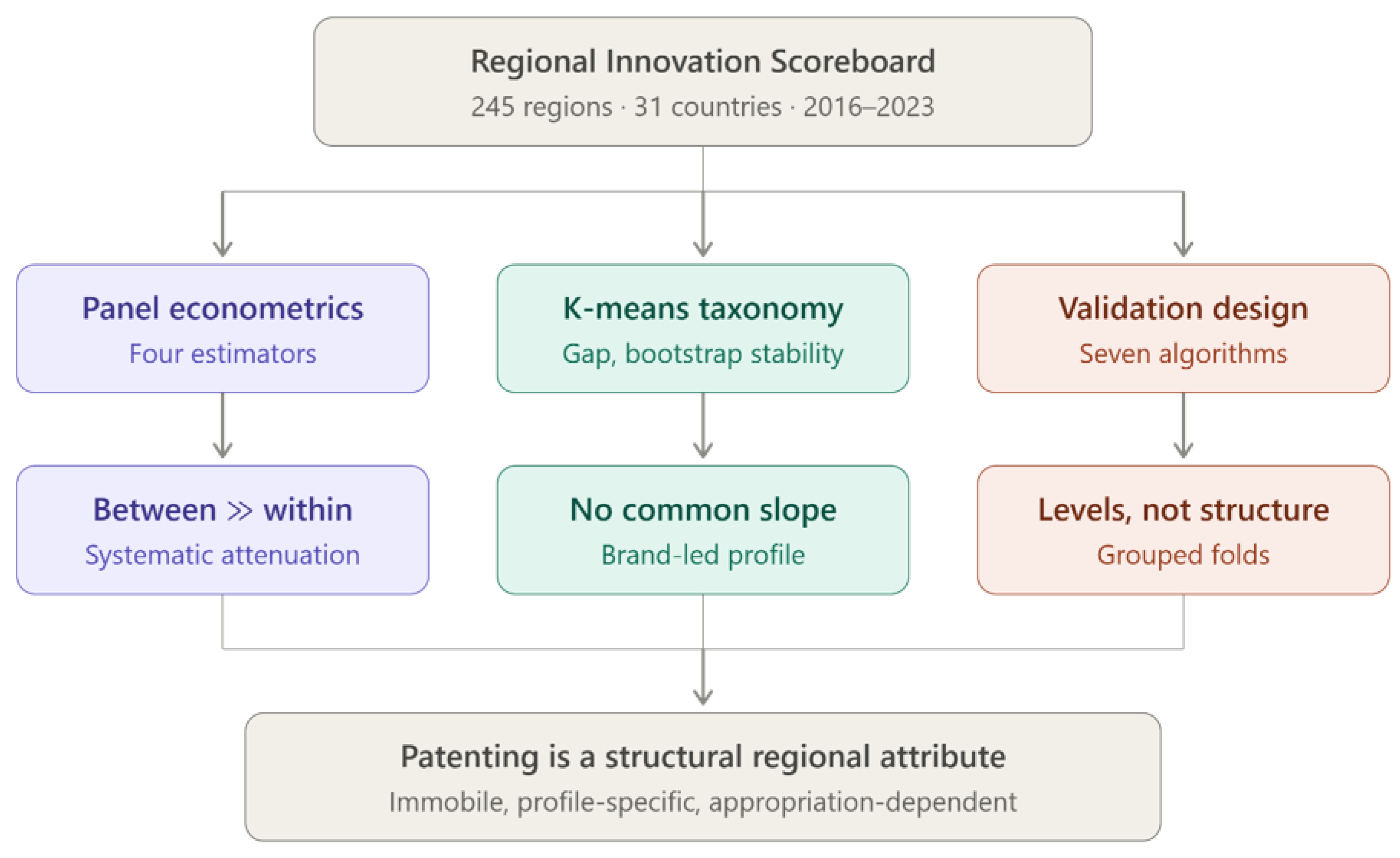
Table 1.
Positioning against the principal strands of the literature.
| Strand and references | Main results | Methodologies | Critical comparison with our findings |
|---|---|---|---|
| Canonical regional KPF — Fritsch and Franke (2004); Moreno et al. (2005); Buesa et al. (2010); Marrocu et al. (2013); Paci et al. (2014), with the extensions cited above | R&D and human capital are the decisive inputs; technological proximity carries most interregional knowledge flow | Cross-section and panel regressions on European NUTS regions, generally with spatial weights | Confirms our ranking of correlates, but identification never separates cross-sectional from temporal variation. Our decomposition shows the between dimension carries almost all the information, making the consensus a between-region result rather than the general one it is presented as |
| Spatial artefact critique — Tappeiner et al. (2008); Guastella and van Oort (2015); Neves and Sequeira (2018) | Spatial autocorrelation is explained by input location; omitting spatial heterogeneity inflates spillovers; estimates depend on the measurement instrument | Spatial econometrics with and without controls for unexplained spatial structure; meta-regression | The closest antecedent of our predictive result, reached by other means. Grouped cross-validation shows the same artefact in a new setting, and the field has not carried this scepticism into algorithmic applications |
| Parameter heterogeneity — Charlot et al. (2015); Kang and Dall'erba (2016a, 2016b); Autant-Bernard and LeSage (2019); Calegari et al. (2017); Mascarini et al. (2023) | Marginal effects of knowledge inputs vary substantially; thresholds and nonlinearities are invisible to standard parametric forms | Semiparametric KPF, geographically weighted regression, heterogeneous-coefficient spatial autoregressive panel | Supports our rejection of common slopes, but partitions by space or by a priori development status. Our data-defined, stability-validated profiles locate the failure in the large intermediate group, precisely where a developed–lagging cut averages over it |
| Efficiency frontier — Li (2009); Niebuhr (2010); Perret (2019); Yan and Sun (2022); Hussinger and Palladini (2024) | Regions differ in how efficiently they convert inputs into inventions, and the determinants of that efficiency are identifiable | Data envelopment analysis and stochastic frontier estimation on regional aggregates | Comes nearest to admitting qualitative difference, but expresses it as distance from a common frontier, presupposing that all regions attempt the same conversion. Our brand-led profile is not inefficient at patenting; it is appropriating elsewhere |
| Critique of the device and of measurement — Ó hUallacháin and Leslie (2007); Varga (2017); Crescenzi and Jaax (2017) | The KPF confounds causes and effects; policy impacts are hard to identify with these tools; conclusions travel poorly across institutional settings | Contrast of competing specifications; review of evaluation designs; comparative regional analysis | Shares our concern with what the specification presupposes, but revises the covariates while leaving patenting as the unquestioned output. Our non-circular design addresses the regressor side; the trademark result addresses the output side, which this critique leaves intact |
Note. Strands are analytical rather than exclusive; several studies contribute to more than one. References illustrate each position rather than exhaust it. The final column states this paper's relation to each strand, not an evaluation.
Table 2.
Descriptive statistics and variance decomposition.
| Variable | Mean | Std. dev. | Min | Max | Between S.D. | Within S.D. | Within var. (%) | Skewness | Kurtosis |
|---|---|---|---|---|---|---|---|---|---|
| PCT | 70.24 | 39.60 | 0.00 | 148.18 | 39.27 | 5.65 | 2.03 | 0.387 | 2.144 |
| RDBUS | 76.56 | 36.70 | 0.00 | 157.40 | 36.33 | 5.61 | 2.34 | 0.177 | 2.589 |
| PPCP | 148.18 | 73.76 | 0.00 | 565.54 | 72.18 | 15.81 | 4.59 | 0.536 | 3.262 |
| TM | 88.76 | 54.22 | 0.00 | 245.91 | 52.91 | 12.24 | 5.10 | 0.818 | 3.168 |
Note. N = 1,960 region-year observations, 245 units, T = 8. Values on the RIS normalised scale (EU average = 100). Between standard deviation computed on regional means; within standard deviation on deviations from regional means.
Table 3.
Pearson correlation matrix, pooled observations.
| PCT | RDBUS | PPCP | TM | |
| PCT | 1.000 | 0.770 | 0.654 | 0.448 |
| RDBUS | 0.770 | 1.000 | 0.619 | 0.360 |
| PPCP | 0.654 | 0.619 | 1.000 | 0.512 |
| TM | 0.448 | 0.360 | 0.512 | 1.000 |
Note. N = 1,960 region-year observations.
Table 4.
Variance inflation factors.
| Variable | VIF, between dimension | VIF, pooled observations |
|---|---|---|
| RDBUS | 1.661 | 1.627 |
| PPCP | 1.980 | 1.920 |
| TM | 1.378 | 1.361 |
Note. Computed on regional means (between dimension) and on pooled region-year observations.
Table 5.
Main results: four panel estimators.
| Pooled OLS | Between | Fixed effects | Random effects | |
| RDBUS | 0.6242*** | 0.6352*** | 0.1028*** | 0.2803*** |
| (0.0643) | (0.0671) | (0.0375) | (0.0347) | |
| PPCP | 0.1343*** | 0.1332*** | 0.0318* | 0.0840*** |
| (0.0319) | (0.0334) | (0.0164) | (0.0226) | |
| TM | 0.0905*** | 0.0923*** | 0.0306* | 0.0524*** |
| (0.0298) | (0.0317) | (0.0173) | (0.0170) | |
| Year fixed effects | Yes | Absorbed | Yes | Yes |
| Regional fixed effects | No | No | Yes | Random |
| Standard errors | Clustered | HC1 robust | Clustered | Clustered |
| Observations | 1,960 | 245 | 1,960 | 1,960 |
| Regions | 245 | 245 | 245 | 245 |
| R² | 0.6683 | 0.6868 | 0.0794 (within) | 0.1740 |
| Root MSE | 22.867 | 22.112 | 5.420 | — |
Note. Dependent variable: PCT patent applications. Standard errors in parentheses; *** p < 0.01, ** p < 0.05, * p < 0.10.
Table 6.
Coefficient attenuation across dimensions.
| Variable | Between | Fixed effects | Ratio between/FE | Within variance share (%) |
|---|---|---|---|---|
| RDBUS | 0.6352 | 0.1028 | 6.18 | 2.34 |
| PPCP | 0.1332 | 0.0318 | 4.19 | 4.59 |
| TM | 0.0923 | 0.0306 | 3.02 | 5.10 |
Note. Within variance share reproduced from Table 1.
Table 7.
Random-effects variance decomposition and fit.
| Statistic | Value |
|---|---|
| Between-unit variance component | 499.35 |
| Within-unit variance component | 33.75 |
| Ratio between/within | 14.8 |
| Intra-class correlation (rho) | 0.9367 |
| Theta used in GLS transformation | 0.9085 |
| Within R², year dummies only | 0.0611 |
| Within R², year dummies plus regressors | 0.0794 |
| Net contribution of the three regressors | 0.0182 |
| Overall R², fixed-effects specification | 0.2900 |
Note. Variance components from the random-effects estimation; R² statistics from the fixed-effects specification.
Table 8.
Year fixed effects, fixed-effects specification.
| Year | Coefficient | Std. error | p-value |
|---|---|---|---|
| 2017 | −1.3781 | 0.5066 | 0.0066 |
| 2018 | −2.9712 | 0.5851 | <0.0001 |
| 2019 | −3.1555 | 0.6246 | <0.0001 |
| 2020 | −4.3305 | 0.6257 | <0.0001 |
| 2021 | −4.5104 | 0.6854 | <0.0001 |
| 2022 | −4.6519 | 0.8376 | <0.0001 |
| 2023 | −7.3921 | 0.9069 | <0.0001 |
Note. Reference year 2016. Standard errors clustered by region.
Table 9.
Diagnostic tests.
| Test | Null hypothesis | Statistic | p-value |
|---|---|---|---|
| Ramsey RESET, pooled | Linear functional form adequate | 7.942 | 0.0004 |
| Ramsey RESET, between | Linear functional form adequate | 1.220 | 0.2970 |
| White, pooled | Homoskedastic errors | 310.15 | <0.0001 |
| White, between | Homoskedastic errors | 43.42 | <0.0001 |
| Jarque–Bera, pooled | Normally distributed residuals | 66.62 | <0.0001 |
| Jarque–Bera, between | Normally distributed residuals | 13.58 | 0.0011 |
| Jarque–Bera, fixed effects | Normally distributed residuals | 745.47 | <0.0001 |
| Durbin–Watson, pooled | No first-order autocorrelation | 0.2241 | — |
| Joint significance, between | All slopes equal zero | 176.18 | <0.0001 |
| Joint significance, fixed effects | All slopes equal zero | 17.81 | <0.0001 |
Note. RESET computed on third-order fitted-value powers.
Table 10.
Log–log between specification.
| Variable | Elasticity | Std. error | p-value |
|---|---|---|---|
| RDBUS | 0.5334*** | 0.0769 | <0.0001 |
| PPCP | 0.3769*** | 0.0620 | <0.0001 |
| TM | 0.1087** | 0.0468 | 0.0201 |
| R² | 0.6768 | ||
| Observations | 241 | ||
| Ramsey RESET | 16.337 | <0.0001 | |
| Jarque–Bera | 8.75 | 0.0126 |
Note. Heteroskedasticity-robust (HC1) standard errors. *** p < 0.01, ** p < 0.05, * p < 0.10. Estimated on 241 units after excluding four regions recording a zero on at least one variable.
Table 11.
Internal validation criteria by number of clusters.
| k | R² | Silhouette | Calinski–Harabasz | Davies–Bouldin | Dunn | Max. diameter | Min. separation |
|---|---|---|---|---|---|---|---|
| 2 | 0.465 | 0.389 | 211.3 | 0.988 | 0.055 | 5.73 | 0.314 |
| 3 | 0.584 | 0.299 | 170.2 | 1.211 | 0.058 | 5.94 | 0.341 |
| 4 | 0.659 | 0.318 | 155.2 | 1.101 | 0.084 | 4.60 | 0.385 |
| 5 | 0.701 | 0.279 | 140.8 | 1.159 | 0.071 | 4.60 | 0.327 |
| 6 | 0.725 | 0.271 | 126.3 | 1.203 | 0.064 | 4.01 | 0.255 |
| 7 | 0.749 | 0.233 | 118.2 | 1.273 | 0.052 | 4.60 | 0.241 |
| 8 | 0.769 | 0.246 | 112.8 | 1.237 | 0.068 | 3.53 | 0.241 |
| 9 | 0.784 | 0.237 | 107.2 | 1.188 | 0.036 | 4.01 | 0.145 |
| 10 | 0.796 | 0.227 | 101.9 | 1.178 | 0.037 | 3.52 | 0.130 |
Note. K-Means on 245 standardised regional averages, 100 random initialisations. Higher values indicate better partitions for R², Silhouette, Calinski–Harabasz, Dunn and minimum separation; lower values for Davies–Bouldin and maximum diameter. The row for k = 4 is the adopted solution.
Table 12.
Gap statistic and bootstrap stability by number of clusters.
| k | Gap | Gap criterion | Mean Jaccard | Minimum Jaccard | Clusters with J < 0.75 | Smallest cluster |
|---|---|---|---|---|---|---|
| 2 | 0.883 | −0.0381 | 0.959 | 0.955 | 0 | 107 |
| 3 | 0.955 | −0.0068 | 0.887 | 0.856 | 0 | 63 |
| 4 | 0.995 | 0.0249 | 0.851 | 0.732 | 1 | 27 |
| 5 | 1.005 | 0.0620 | 0.752 | 0.685 | 3 | 24 |
| 6 | 0.974 | 0.0350 | 0.586 | 0.369 | 5 | 23 |
| 7 | 0.972 | 0.0231 | 0.566 | 0.450 | 6 | 16 |
| 8 | 0.977 | 0.0496 | 0.572 | 0.427 | 7 | 10 |
| 9 | 0.961 | 0.0487 | 0.535 | 0.444 | 9 | 12 |
| 10 | 0.944 | 0.0315 | 0.498 | 0.322 | 10 | 11 |
Note. The gap statistic is computed against 50 reference datasets drawn uniformly over the data envelope (Tibshirani, Walther and Hastie, 2001); the reported criterion is Gap(k) − Gap(k+1) + s(k+1), which selects the smallest k with a non-negative value. The Jaccard index measures cluster stability over 200 non-parametric bootstrap resamples (Hennig, 2007), under the convention: above 0.85 highly stable; 0.75–0.85 stable; 0.60–0.75 uncertain; below 0.60 unreliable. The row for k = 4 is the adopted solution.
Table 16.
Distribution of clusters by country.
| Country | Cluster 1 Leading | Cluster 2 Peripheral | Cluster 3 Intermediate | Cluster 4 Trademark | Total |
|---|---|---|---|---|---|
| Germany | 20 | 0 | 16 | 2 | 38 |
| Italy | 1 | 6 | 9 | 5 | 21 |
| Spain | 0 | 9 | 4 | 6 | 19 |
| Poland | 0 | 14 | 2 | 1 | 17 |
| France | 2 | 2 | 10 | 0 | 14 |
| Greece | 0 | 12 | 1 | 0 | 13 |
| Netherlands | 5 | 0 | 6 | 1 | 12 |
| United Kingdom | 2 | 0 | 9 | 1 | 12 |
| Czechia | 0 | 2 | 5 | 1 | 8 |
| Hungary | 0 | 5 | 3 | 0 | 8 |
| Romania | 0 | 8 | 0 | 0 | 8 |
| Sweden | 4 | 0 | 4 | 0 | 8 |
| Norway | 2 | 2 | 3 | 0 | 7 |
| Portugal | 0 | 4 | 2 | 1 | 7 |
| Switzerland | 6 | 0 | 0 | 1 | 7 |
| Bulgaria | 0 | 5 | 0 | 1 | 6 |
| Denmark | 4 | 0 | 1 | 0 | 5 |
| Finland | 4 | 1 | 0 | 0 | 5 |
| Croatia | 0 | 1 | 3 | 0 | 4 |
| Serbia | 0 | 4 | 0 | 0 | 4 |
| Slovakia | 0 | 3 | 1 | 0 | 4 |
| Austria | 3 | 0 | 0 | 0 | 3 |
| Belgium | 1 | 0 | 1 | 1 | 3 |
| Ireland | 0 | 0 | 3 | 0 | 3 |
| Lithuania | 0 | 1 | 0 | 1 | 2 |
| Slovenia | 0 | 0 | 1 | 1 | 2 |
| Cyprus | 0 | 0 | 0 | 1 | 1 |
| Estonia | 0 | 0 | 0 | 1 | 1 |
| Latvia | 0 | 1 | 0 | 0 | 1 |
| Luxembourg | 0 | 0 | 0 | 1 | 1 |
| Malta | 0 | 0 | 0 | 1 | 1 |
| Total | 54 | 80 | 84 | 27 | 245 |
Note. Number of regional units by country and cluster. Cyprus, Estonia, Latvia, Luxembourg and Malta appear as national units, not being disaggregated regionally in the Regional Innovation Scoreboard.
Table 17.
Out-of-sample coefficient of determination under three validation designs, full predictor set.
Table 17.
Out-of-sample coefficient of determination under three validation designs, full predictor set.
| Algorithm | Random partition | Grouped k-fold | Temporal holdout | Random − grouped |
|---|---|---|---|---|
| Linear regression | 0.8036 | 0.7788 | 0.7728 | 0.0248 |
| Lasso | 0.7978 | 0.7792 | 0.7565 | 0.0185 |
| k-NN (k = 1) | 0.9563 | 0.6738 | 0.9446 | 0.2824 |
| k-NN (k = 5) | 0.9460 | 0.7557 | 0.9182 | 0.1904 |
| Decision tree | 0.8891 | 0.6807 | 0.8608 | 0.2083 |
| Random forest | 0.9467 | 0.8132 | 0.9233 | 0.1335 |
| Gradient boosting | 0.9295 | 0.8337 | 0.9129 | 0.0958 |
Note. Twenty predictors, all Regional Innovation Scoreboard indicators non-circular with respect to PCT. Five folds in both cross-validation designs; the temporal holdout trains on 1,470 observations and evaluates on 490. Continuous predictors are standardised within each training fold for the linear, penalised and nearest-neighbour models. The final row is the best-performing algorithm under grouped validation.
Table 18.
Out-of-sample error under three validation designs, full predictor set.
| Algorithm | RMSE random | RMSE grouped | RMSE holdout | MAE grouped | MAE holdout |
|---|---|---|---|---|---|
| Linear regression | 17.51 | 18.48 | 18.53 | 14.61 | 15.17 |
| Lasso | 17.77 | 18.47 | 19.19 | 14.76 | 15.64 |
| k-NN (k = 1) | 8.25 | 22.45 | 9.15 | 16.28 | 5.20 |
| k-NN (k = 5) | 9.17 | 19.43 | 11.12 | 14.27 | 7.53 |
| Decision tree | 13.09 | 22.23 | 14.51 | 16.46 | 9.07 |
| Random forest | 9.06 | 16.95 | 10.77 | 12.78 | 7.58 |
| Gradient boosting | 10.48 | 16.03 | 11.48 | 12.04 | 8.83 |
Note. Errors on the RIS index scale, where the European Union average equals 100 and the dependent variable ranges from 0 to 148.18. Same folds and standardisation as Table 16.
Table 19.
Out-of-sample performance under three validation designs, parsimonious predictor set.
| Algorithm | Random partition | Grouped k-fold | Temporal holdout | RMSE grouped | Random − grouped |
|---|---|---|---|---|---|
| Linear regression | 0.6523 | 0.6452 | 0.5904 | 23.27 | 0.0071 |
| Lasso | 0.6523 | 0.6452 | 0.5906 | 23.27 | 0.0071 |
| k-NN (k = 1) | 0.7175 | 0.2649 | 0.5792 | 33.77 | 0.4526 |
| k-NN (k = 5) | 0.7768 | 0.4610 | 0.6543 | 28.92 | 0.3157 |
| Decision tree | 0.6150 | 0.2625 | 0.5020 | 33.84 | 0.3525 |
| Random forest | 0.7968 | 0.5347 | 0.6705 | 26.88 | 0.2621 |
| Gradient boosting | 0.7417 | 0.5859 | 0.6377 | 25.27 | 0.1558 |
Note. Three predictors only — business R&D expenditure, public–private co-publications and trademark applications — corresponding to the specification retained in the econometric analysis. Coefficients of determination in the first three columns, root mean squared error in the fourth.
Table 20.
Fold-level coefficient of determination under grouped k-fold validation, full predictor set.
Table 20.
Fold-level coefficient of determination under grouped k-fold validation, full predictor set.
| Algorithm | Fold 1 | Fold 2 | Fold 3 | Fold 4 | Fold 5 | Mean | Std. dev. |
|---|---|---|---|---|---|---|---|
| Linear regression | 0.823 | 0.756 | 0.810 | 0.742 | 0.763 | 0.779 | 0.032 |
| Lasso | 0.818 | 0.764 | 0.810 | 0.765 | 0.739 | 0.779 | 0.030 |
| k-NN (k = 1) | 0.754 | 0.629 | 0.679 | 0.674 | 0.633 | 0.674 | 0.045 |
| k-NN (k = 5) | 0.819 | 0.735 | 0.751 | 0.749 | 0.724 | 0.756 | 0.033 |
| Decision tree | 0.731 | 0.627 | 0.712 | 0.703 | 0.631 | 0.681 | 0.043 |
| Random forest | 0.823 | 0.725 | 0.841 | 0.854 | 0.823 | 0.813 | 0.046 |
| Gradient boosting | 0.847 | 0.793 | 0.853 | 0.871 | 0.805 | 0.834 | 0.030 |
Note. Each fold withholds approximately 49 regions and all eight of their yearly observations.
Table 21.
Permutation importance under grouped k-fold validation, random forest.
| Predictor | Mean increase in RMSE | Std. dev. across folds | Within-region variance (%) | Correlation with PCT |
|---|---|---|---|---|
| RDBUS | 15.989 | 1.578 | 2.3 | 0.770 |
| TOP10PUB | 8.984 | 1.129 | 10.3 | 0.619 |
| LLL | 2.880 | 0.829 | 0.1 | 0.520 |
| DES | 1.254 | 0.110 | 9.2 | 0.496 |
| INNOEMP | 0.870 | 0.425 | 7.2 | 0.693 |
| DIGSK | 0.718 | 0.544 | 0.4 | 0.345 |
| PPCP | 0.501 | 0.153 | 4.6 | 0.654 |
| KIAEMP | 0.485 | 0.535 | 0.1 | 0.504 |
| PMEM | 0.341 | 0.126 | 9.3 | 0.445 |
| ICTSP | 0.231 | 0.277 | 2.4 | 0.450 |
| RDPUB | 0.175 | 0.127 | 3.2 | 0.474 |
| IEPE | 0.161 | 0.089 | 8.4 | 0.351 |
| PTE | 0.157 | 0.253 | 0.4 | 0.288 |
| NRDIE | 0.155 | 0.056 | 30.0 | −0.050 |
| SMEBPI | 0.051 | 0.056 | 23.1 | 0.461 |
| TM | 0.038 | 0.152 | 5.1 | 0.448 |
| SMECOLL | 0.025 | 0.046 | 17.8 | 0.396 |
| NEWSALES | 0.022 | 0.025 | 36.8 | 0.221 |
| SMEPI | 0.016 | 0.014 | 19.6 | 0.582 |
| ISCP | 0.010 | 0.125 | 3.6 | 0.517 |
Note. Importance is the average increase in root mean squared error when a predictor’s values are randomly permuted in the held-out fold, over ten repetitions in each of five grouped folds. Importance is conditional on the remaining nineteen predictors.
Table 22.
Summary of the main results.
| Finding | Evidence | Method | Implication |
|---|---|---|---|
| Business research dominates | Positive and significant under all four estimators; highest permutation importance of twenty indicators | Panel estimation; random-forest importance under grouped folds | Confirms the knowledge production consensus, and independently of functional form |
| Explanatory content lies between regions | Within-region variance of 2–5 per cent; attenuation ordered inversely to temporal information | Variance decomposition; four panel estimators | The default within estimator is applied to a thin, partly interpolated residual |
| The average relationship describes no group | Aggregate coefficient of 0.635 against a subgroup range of −0.002 to 0.394; no significance in the largest cluster | K-Means partition validated by gap statistic and bootstrap stability; cluster-wise regression | Uniform elasticities are miscalibrated for most regions and inert for the modal one |
| Appropriation takes distinct forms | Twenty-seven regions with trademarks far above patents, drawn from every performance tier | Cluster profiles on the original scale; comparison with the official classification | A patent-only measure misreads regions whose advantage is non-technological |
| Predictive gains rest on levels, not structure | Nearest neighbours loses 0.28 of R² under grouped folds; linear models lose 0.02 | Seven algorithms under random, grouped and temporal designs | Accuracy reported without respecting panel structure is overstated |
Note. Coefficients on the RIS normalised scale (EU average = 100). Subgroup range refers to the coefficient on business R&D expenditure estimated separately within the four clusters.
Table 23.
Differentiated policy implications by regional profile.
| Target group | Binding constraint identified | Instrument implied | Evaluation horizon |
|---|---|---|---|
| Leading regions (54) | None internal; competition is with US and Chinese frontier firms | Scale-up capital and concentration of frontier capability, not additional research subsidy | Continuous, against non-European benchmarks |
| Peripheral regions (80), largely Eastern and Southern | Level of business research input; the transmission mechanism functions | Sustained increase in corporate research capacity and absorptive capacity | 15–20 years, on input and institutional indicators |
| Intermediate regions (84) | Conversion of research into protected output; the association is undetectable | Institutional quality, university–industry interface, risk capital — not more research spending alone | 15–20 years, on linkage indicators |
| Brand-led regions (27), across all tiers | Measurement, not capability; appropriation runs through trademarks | Design, branding and service-innovation instruments; revised performance metrics | Immediate reclassification; then as above |
Note. Profiles as identified in Section 5. Group sizes in parentheses. The evaluation horizon column follows from the variance decomposition reported in Section 4: within-region variation over eight years carries too little information to support shorter assessment cycles based on patenting outcomes.
Disclaimer/Publisher’s Note: The statements, opinions and data contained in all publications are solely those of the individual author(s) and contributor(s) and not of MDPI and/or the editor(s). MDPI and/or the editor(s) disclaim responsibility for any injury to people or property resulting from any ideas, methods, instructions or products referred to in the content. |
© 2026 by the authors. Licensee MDPI, Basel, Switzerland. This article is an open access article distributed under the terms and conditions of the Creative Commons Attribution (CC BY) license (http://creativecommons.org/licenses/by/4.0/).
Copyright: This open access article is published under a Creative Commons CC BY 4.0 license, which permit the free download, distribution, and reuse, provided that the author and preprint are cited in any reuse.