
Submitted:
14 August 2026
Posted:
17 August 2026
You are already at the latest version
Abstract
Many economic time series are compositions: educational attainment shares, waste treatment routes, energy mixes, sectoral employment. Forecasters usually transform such series to log-ratio coordinates and apply generic univariate or multivariate methods, imposing no economic restriction on how the parts move. Evolutionary game theory offers an obvious candidate restriction, since replicator dynamics makes the growth rate of a share proportional to its relative payoff advantage. We take that restriction seriously as a forecasting device. A discrete-time replicator-mutator map with linear payoffs and a common congestion term is estimated under three pooling regimes, country-specific, fully pooled, and shrunk between the two, and raced against five log-ratio benchmarks in an expanding-window rolling-origin design on three Eurostat panels. The central finding is that the pooling regime governs accuracy more strongly than the choice between structural and statistical models. Moving from country-specific to pooled parameters reduces the mean absolute scaled error by 27.8% on educational attainment and by 15.3% to 19.8% on municipal waste routes, whereas the best structural specification differs from the best benchmark by only 1.3% on educational attainment. Structural specifications enter the model confidence set on the attainment panel but not on the waste panels, where no-change forecasts dominate. Win rates diverge sharply from mean losses, which suggests combination rather than selection.
Keywords:
compositional time series
; replicator-mutator dynamics
; forecast evaluation
; parameter pooling
; shrinkage
; model confidence set
; evolutionary game theory
1. Introduction
A large share of the quantities that economists forecast are not levels but shares. The educational composition of the working-age population, the split of municipal waste across treatment routes, the fuel mix of an electricity system, the distribution of employment across contract types: in each case the object of interest is a vector of non-negative parts that sums to one. Such vectors live on the unit simplex, and the simplex is not a vector space under ordinary addition. Forecasting them with methods designed for unconstrained series risks predictions that are negative, that fail to add up, or that drift outside the feasible region at long horizons.
The standard response, following Aitchison [1,2], is to move to log-ratio coordinates, forecast there with a generic method, and map the result back. This solves the coherence problem completely and cheaply. What it does not do is impose any economic content. A vector autoregression in additive log-ratio coordinates treats the composition as an arbitrary multivariate process; nothing in its structure says that a part should grow when the activity it represents is doing comparatively well.
Economics has a natural candidate for exactly that restriction. Replicator dynamics, introduced by Taylor and Jonker [3] and developed into the standard apparatus of evolutionary game theory by Hofbauer and Sigmund [4], Weibull [5] and Sandholm [6], makes the growth rate of a share proportional to the gap between its payoff and the population average payoff. Its behavioural microfoundations are well understood: it arises from imitation of successful others under bounded rationality [7], and from payoff-monotone revision protocols more generally [6]. Adding mutation, in the sense of Nowak, Komarova and Niyogi [8] and Komarova [9], introduces a small flow toward strategies that are not currently doing well, which can be read as experimentation, entry, or simply the failure of imitation to be perfect.
This paper asks whether that restriction earns its keep out of sample. The question is a forecasting question and we treat it as one, with a rolling-origin design, a panel of benchmarks, scale-free losses, and formal tests of equal predictive ability. The answer we obtain is not the one the framing invites, and it is more interesting than a simple yes.
Our contribution is threefold. First, we specify a discrete-time replicator-mutator map with linear payoffs and a common congestion term that has only K + 1 free parameters for a K-part composition, and we show how to estimate it by conditional least squares in Aitchison geometry so that its forecasts are coherent by construction. Second, we embed the model in three pooling regimes, country-specific, fully pooled, and shrunk between the two with the shrinkage weight selected on training data alone, and race all three against five log-ratio benchmarks. Third, and most importantly, we document that the pooling regime is a first-order determinant of accuracy while the structural-versus-statistical distinction is second-order. Across three Eurostat panels the spread within the structural family, generated purely by how parameters are shared across countries, is 18.1% to 38.5% in mean absolute scaled error, whereas the gap between the best structural specification and the best benchmark is 1.3% on one panel and 11.5% to 12.0% on the others.
We also report two findings that qualify any simple accuracy ranking. Win rates and mean losses point in different directions: the pooled structural model produces the lowest loss on 26.4% of forecast events on the attainment panel, more than twice the share of any competitor, without having the lowest average loss. And on both waste panels the no-change benchmark is alone in the model confidence set at almost every horizon, so that the honest conclusion for those data is that no dynamic model, structural or statistical, extracts usable signal.
Section 2 places the paper in the literature. Section 3 sets out the model, Section 4 the estimator, Section 5 the evaluation design. Section 6 reports Monte Carlo evidence on parameter recovery and on behaviour under correct and incorrect specification. Section 7 describes the data and Section 8 the results. Section 9 and Section 10 discuss and conclude.
2. Related Work
Three literatures meet here. The first is compositional data analysis. Aitchison [1,2] established the log-ratio approach and the geometry that goes with it; Egozcue and co-authors [10] added the isometric transform, and Pawlowsky-Glahn, Egozcue and Tolosana-Delgado [11] provide the modern treatment. Applications to time series are comparatively recent. Kynčlová, Filzmoser and Hron [12] study vector autoregressions for compositional series, and Snyder and co-authors [13] develop a state space approach to compositional forecasting. Our benchmarks are drawn from this tradition and our losses are defined in its geometry.
The second is evolutionary dynamics in economics. Beyond the foundational treatments already cited [3,4,5,6], the relevant strand for us is the one that treats replicator and replicator-mutator equations as models of learning and adaptation in populations of boundedly rational agents rather than as biological analogies [7,9,14,15]. Applications are overwhelmingly theoretical or estimated in sample. Treating the dynamics as an out-of-sample forecasting device, and holding it to the evaluation standards of the forecasting literature, appears to be new.
The third is the forecasting methodology literature itself, and in particular its long insistence that simple methods are hard to beat and that claims of accuracy must be established with proper protocols. Hyndman and Koehler [16] gave the scaled error measure we use, Diebold and Mariano [17] and Harvey, Leybourne and Newbold [18] the equal-accuracy test and its small-sample correction, Hansen, Lunde and Nason [19] the model confidence set, and Giacomini and White [20] the conditional version of the accuracy comparison. Elliott and Timmermann [21] survey the field. Our finding that pooling dominates structure is a version, in a new setting, of the recurring lesson that variance reduction usually buys more than sophistication.
3. A Structural Forecasting Model
3.1. Payoffs, Selection and Exploration
Let be a composition of strategies observed at annual frequency, so that and the parts sum to one. Payoffs are linear in the composition with a strategy-specific intercept and a common congestion term,
The normalisation is required because only payoff differences matter. The parameter carries the economics: means that a strategy becomes less attractive the more of the population uses it, which is congestion, crowding, or diminishing returns to a route; means increasing returns, so that adoption is self-reinforcing.
Selection is the discrete replicator map with exponential fitness, and exploration enters as uniform mutation at rate ,
The exponential form keeps the iterates strictly inside the simplex and is numerically stable, which matters when the map is iterated five steps ahead from many origins. A selection intensity multiplying the payoffs is not separately identified from the scale of and is normalised to one throughout.
3.2. Rest Points and the Role of the Mutation Term
For the vertices of the simplex are rest points, and the long-horizon forecast of a pure replicator model is generically a corner. For this is no longer possible: applying the map at a vertex returns , so no vertex is a rest point. As the map collapses to the constant map at the barycentre. The mutation parameter therefore interpolates between the selection attractor and the centre of the simplex, and in forecasting terms it operates exactly as a shrinkage device: larger pulls multi-step forecasts toward the uniform composition, reducing forecast variance at the cost of bias.
Numerically, with , and , the interior rest point moves from at to at , a displacement toward the barycentre. This is a small effect at one step and a large one at long horizons, since it is the limit point rather than the local slope that it relocates.
Rest points need not be unique. When the payoff structure is self-reinforcing and the map can support several stable configurations, so that the same estimated model implies different long-run compositions from different starting points. We report the number of numerically located rest points for every estimated unit in Section 8.5.
3.3. Parameter Counts
The specification has intercepts, one congestion parameter and one mutation parameter, hence free parameters. Table 1 compares this with the log-ratio benchmarks on coordinates. The advantage is modest at and grows quickly, because the autoregressive parameterisation is quadratic in the number of coordinates while the structural one is linear in the number of parts.
3.4. Three Pooling Regimes
Let collect the parameters, with so that the vector is unconstrained. For a panel of units we consider three regimes. Under the country-specific regime, is estimated on unit ’s training window alone. Under the pooled regime a single is estimated on all units’ training data jointly. Under the shrunk regime,
with chosen for each unit and each origin by an inner hold-out that uses only the training window, never the evaluation sample. Because the combination is taken in the unconstrained parameterisation, the implied remains in the unit interval by construction.
4. Estimation and Forecast Construction
Parameters are estimated by conditional least squares in Aitchison geometry. Writing for the one-step map, the estimator minimizes
where is the centred log-ratio transform and the outer sum runs over whichever units the pooling regime includes. Minimisation uses a bounded quasi-Newton routine from twelve starting values, of which one is the no-selection, no-congestion point and the remainder are drawn at random, and the best local optimum is retained. Multi-step forecasts are produced by iterating the estimated map from the last observed composition, which yields a coherent path on the simplex at every horizon without any post hoc renormalisation.
Zero parts are replaced multiplicatively before any log-ratio operation, with the replaced mass set to in proportion units and the remaining parts rescaled so that the composition still closes to one. The same replacement is applied identically to every model, so it cannot favour one competitor over another.
5. Forecast Evaluation Design
5.1. Benchmarks
Five benchmarks are applied to the additive log-ratio coordinates of the composition and mapped back through the inverse transform, so that their forecasts are coherent exactly as the structural model’s are. The no-change benchmark repeats the last observed composition. The random walk with drift extrapolates the average log-ratio change over the training window. Univariate ARIMA models are fitted per coordinate with the order selected from a curated grid by corrected Akaike information. Exponential smoothing is fitted per coordinate with and without a damped additive trend, again selected by corrected Akaike information [22]. A vector autoregression is fitted to the full log-ratio vector with lag order chosen by Akaike information. Whenever a training window is too short or an optimiser fails, the routine falls back to the random walk with drift.
5.2. Losses
Two losses are reported. The first is the Aitchison distance between the realised and predicted composition, which is the natural metric of the sample space. The second is the mean absolute scaled error of Hyndman and Koehler [16], computed on log-ratio coordinates, averaged over coordinates, and scaled by the in-sample mean absolute one-step no-change error of the corresponding training window. The scaled error is the primary measure because it is comparable across panels of different volatility.
5.3. Rolling Origin
The design is an expanding window. For each unit, the model is re-estimated at every origin using only data up to that origin, and forecasts are produced for horizons one through five, truncated at the end of the sample. Crucially this applies to the structural model as well: the shrinkage weight, the pooled parameter vector and the unit-specific parameter vector are all recomputed at every origin from training data alone.
5.4. Tests of Equal Predictive Ability
Pairwise comparisons use the Diebold-Mariano statistic [17] with the small-sample correction of Harvey, Leybourne and Newbold [18]. Because forecast errors are correlated within a country and across origins, we also report a bootstrap p-value that resamples whole countries with replacement, which is the relevant clustering for a panel of national statistics. Finally we compute the model confidence set of Hansen, Lunde and Nason [19] in its range-statistic form at the 10% level, which identifies the subset of models that cannot be distinguished from the best.
6. Monte Carlo Evidence
6.1. Parameter Recovery
Panels of forty units were generated from the structural map with logistic-normal observation noise on log-ratio coordinates, varying the sample length and the noise standard deviation. Table 2 reports the bias and root mean squared error of the estimated congestion and mutation parameters.
The congestion parameter is recovered well: at low noise the median relative error is within a third of one percent of zero at every sample length, and the large root mean squared errors at higher noise are driven by a small number of units for which the objective is nearly flat, not by a systematic tilt. The mutation parameter is a different matter. Its bias is positive in every configuration and its median relative error deteriorates sharply with noise, reaching a factor of seven at the noisiest configuration. The mechanism is transparent: observation noise on the simplex is, to a first approximation, indistinguishable from mutation, so the estimator absorbs measurement error into . The implication for interpretation is important and we return to it in Section 9: the estimated should be read as a reduced-form smoothing parameter, not as a behavioural exploration rate.
6.2. Correct and Incorrect Specification
Two further experiments run the full evaluation machinery on generated data. In the first, twelve units of twenty-six annual observations are generated from the structural map. In the second, they are generated from a log-ratio VAR(1) with drift, a process outside the structural family. Table 3 reports mean absolute scaled errors averaged over horizons.
Under correct specification the country-specific structural model wins, as it must, and the fully pooled version is badly hurt because the generated units genuinely have heterogeneous parameters. Under misspecification the VAR wins, again as it must, and the structural model degrades but does not collapse: the shrunk version remains ahead of ARIMA, of the random walk with drift, and of both other structural regimes. These experiments establish that the machinery is wired correctly and that the pooling regime is capable of moving accuracy in either direction depending on the true degree of heterogeneity. They do not, of course, tell us which direction applies to real data.
7. Data
Three panels are constructed from Eurostat online datasets, restricted to the longest run of consecutive annual observations from 2000 onward with at least eighteen years, and with the European Union and euro area aggregates removed so that every unit is a country.
The attainment panel uses population by educational attainment level for ages 25 to 64, both sexes, in percent (Eurostat online data code edat_lfse_03), partitioned into ISCED 2011 levels 0 to 2, 3 to 4, and 5 to 8. These three parts are an exact partition and sum to 100 in the raw data to within rounding at every observation.
The waste panels use municipal waste by treatment operation in thousand tonnes (Eurostat online data code env_wasmun). The three-route version partitions treated municipal waste into recycling including composting and digestion, incineration including energy recovery, and landfill and other disposal; these three routes account for 99.6% of reported treated municipal waste on average. The four-route version splits recycling into material recycling and composting with digestion, giving a four-part composition on the same countries and years and allowing the parameter-count advantage of Table 1 to be exercised.

Table 4.
Panel descriptives. Zero cells are parts reported as zero and subject to multiplicative replacement.
Table 4.
Panel descriptives. Zero cells are parts reported as zero and subject to multiplicative replacement.
| Panel | Parts | Countries | Years | Observations | Zero cells | Origins | Target years |
|---|---|---|---|---|---|---|---|
| Attainment | 3 | 33 | 2000-2025 | 834 | 0 (0.0%) | 438 | 2012-2025 |
| Waste, 3 routes | 3 | 25 | 2000-2024 | 609 | 111 (6.1%) | 309 | 2012-2024 |
| Waste, 4 routes | 4 | 25 | 2000-2024 | 609 | 163 (6.7%) | 309 | 2012-2024 |
The contrast between the panels is deliberate. Educational attainment compositions are strongly and monotonically trending across Europe over this period, as the low-attainment share falls and the tertiary share rises. Municipal waste routes are noisier, subject to reporting revisions, and contain genuine structural zeros for countries that operate no incineration capacity. The minimum training window is twelve observations throughout.
8. Results
8.1. Accuracy and the Model Confidence Set
Table 5 reports mean absolute scaled errors by horizon on the attainment panel. The random walk with drift is the most accurate model overall, with the pooled structural specification 1.3% behind it and ARIMA a further step back. The country-specific structural specification is markedly worse, and the no-change benchmark is worst of all, which is what a strongly trending composition should produce.
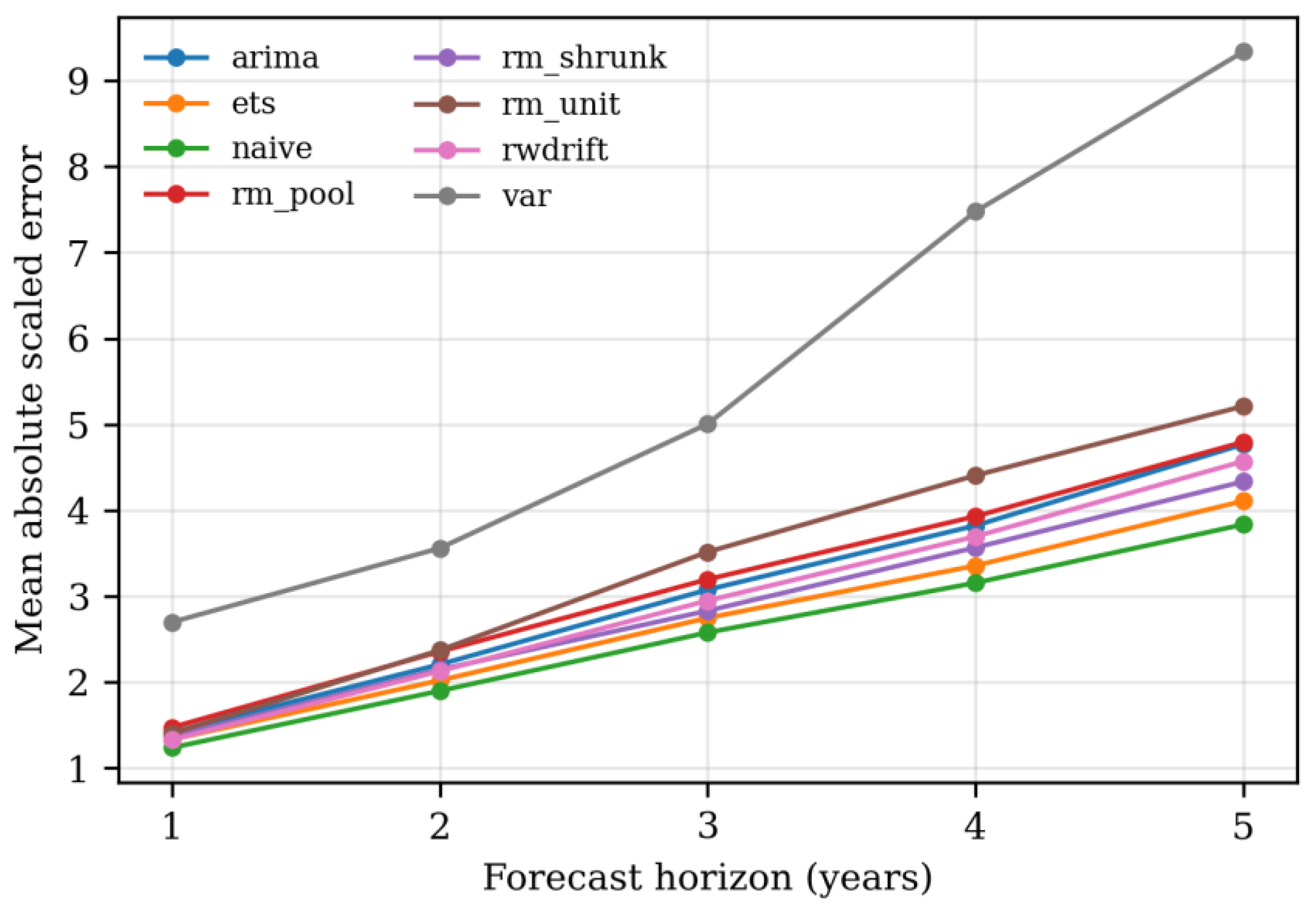
Table 6 reports the same quantity for the two waste panels. Here the ordering inverts completely: the no-change benchmark is the most accurate model at every horizon on both panels, and every dynamic model loses to it. Among the dynamic models the shrunk structural specification is the best on the four-route panel and second best on the three-route panel, and it beats the VAR by a very wide margin, but this is a ranking among losers.
Figure 1.
Mean absolute scaled error by forecast horizon, educational attainment panel, 33 countries, expanding-window rolling origin.
Figure 1.
Mean absolute scaled error by forecast horizon, educational attainment panel, 33 countries, expanding-window rolling origin.
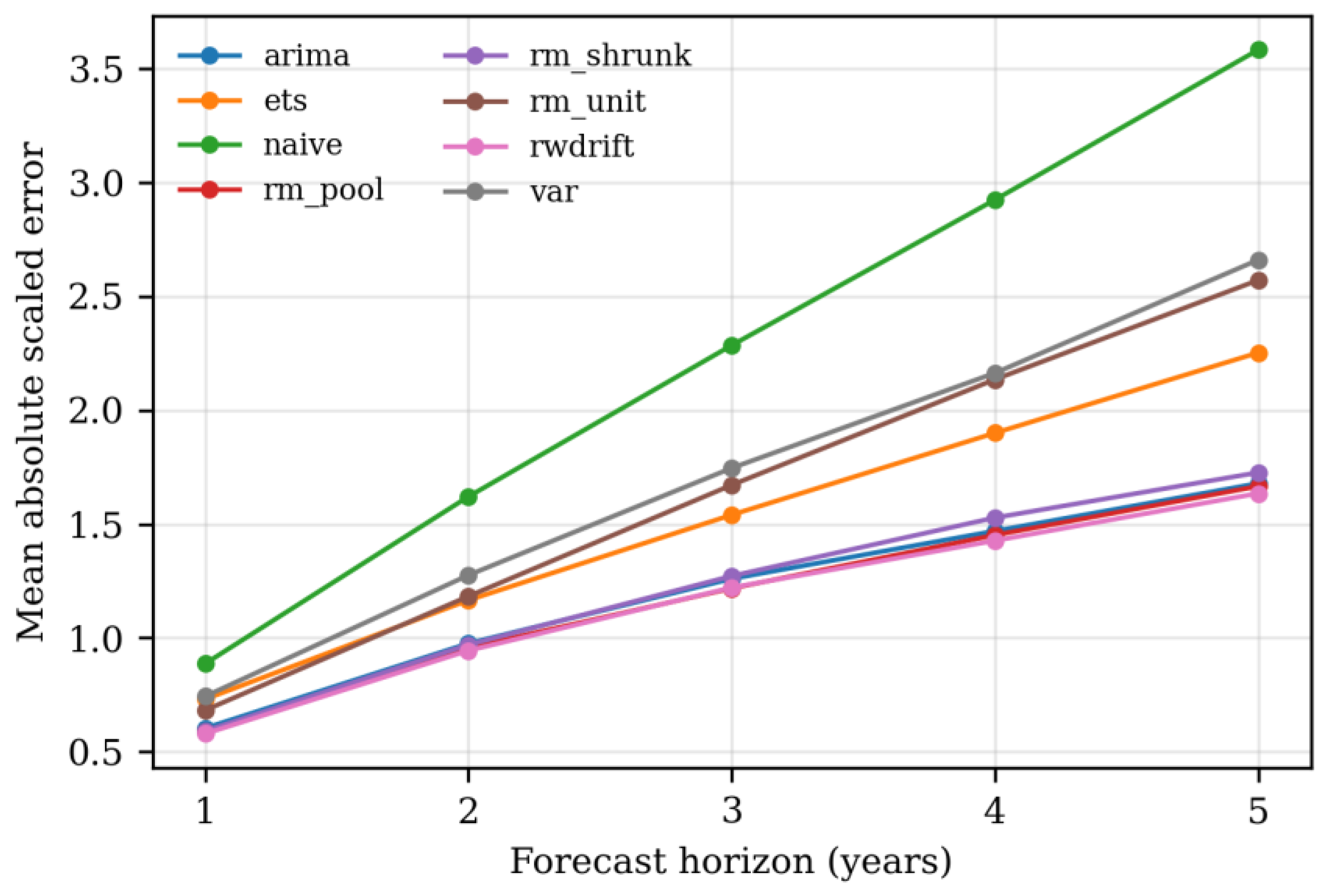
Figure 2.
Mean absolute scaled error by forecast horizon, three-route municipal waste panel, 25 countries.
Figure 2.
Mean absolute scaled error by forecast horizon, three-route municipal waste panel, 25 countries.
The model confidence sets sharpen the picture. On the attainment panel the set contains the random walk with drift, the pooled structural model and the shrunk structural model at horizons one and two, and the first two of these at horizons three to five. The structural model is therefore statistically indistinguishable from the best available forecast on this panel, without being better than it. On both waste panels the set contains the no-change benchmark alone at every horizon, with the single exception of horizon three on the four-route panel, where the shrunk structural model survives alongside it.
Formal pairwise tests agree. Against the random walk with drift on the attainment panel, the corrected Diebold-Mariano statistics for the shrunk structural model range from -1.45 to -0.87 across horizons, with p-values between 0.148 and 0.383 and country-clustered bootstrap p-values between 0.168 and 0.478: no significant difference in either direction. Against the no-change benchmark on the waste panels the structural model is significantly worse at the shortest horizons and insignificantly worse thereafter.
8.2. The Pooling Regime Dominates the Model Class
The central result of the paper is visible by comparing within-family and between-family spreads. Table 7 sets the three pooling regimes against the best benchmark on each panel.
Figure 3.
Left: mean absolute scaled error of the three pooling regimes on each panel, with the best benchmark shown as a dashed line. Right: share of forecast events on which each model attains the lowest scaled error.
Figure 3.
Left: mean absolute scaled error of the three pooling regimes on each panel, with the best benchmark shown as a dashed line. Right: share of forecast events on which each model attains the lowest scaled error.
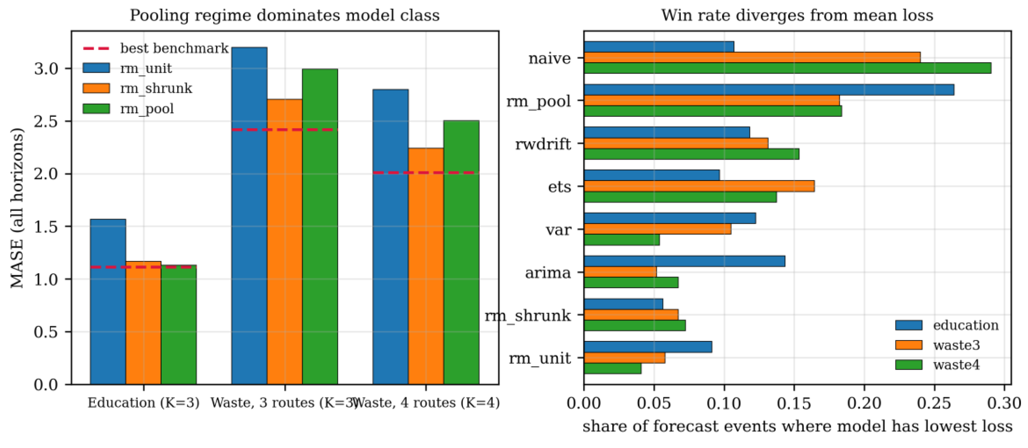
Two comparisons matter. First, sharing parameters across countries reduces error by 27.8% on the attainment panel and by 15.3% and 19.8% on the waste panels. Second, the gap between the best structural specification and the best benchmark is 1.3%, 12.0% and 11.5% respectively. On the attainment panel the effect of the pooling decision is therefore more than twenty times the effect of the structural-versus-statistical decision; on the waste panels the two are of comparable magnitude, with pooling still larger on the four-route panel. In no case is the model class the dominant consideration.
The direction of the pooling effect deserves emphasis because it reverses the Monte Carlo. In the correctly specified simulation, where units genuinely had heterogeneous parameters and the noise was mild, country-specific estimation won and full pooling was badly beaten. In the real panels, country-specific estimation is the worst structural specification everywhere. The reconciliation is a standard bias-variance argument: at twelve to twenty-five annual observations per country, the sampling variance of four or five country-specific parameters swamps whatever heterogeneity bias pooling introduces. What the simulation shows is that this is not a foregone conclusion but a property of the sample sizes and noise levels that official annual statistics actually deliver.
8.3. Win Rates Diverge from Mean Losses
Mean losses are not the only summary of relative accuracy. Table 8 reports, for each model, the fraction of individual forecast events, defined as a country by origin by horizon triple, on which that model attains the lowest scaled error.
On the attainment panel the pooled structural model has the highest win rate by a wide margin, 26.4% against 14.4% for the next model, yet it does not have the lowest mean loss. On both waste panels it is second only to the no-change benchmark, and again well ahead of everything else. The reading is that the structural model is right more often than its competitors but wrong by more when it is wrong, which is exactly what a model with a strong long-run restriction should do: when the restriction fits the country, iterating a bounded map is very accurate, and when it does not, the iterated map runs away from the data.
This pattern is an argument for combination rather than selection. A model that wins a quarter of the events carries information that a model with the lowest average loss does not necessarily contain, and the standard remedy for asymmetric loss profiles of this kind is to average rather than to choose.
8.4. What the Shrinkage Weight Selects
The inner hold-out chooses the shrinkage weight from three values on training data alone. Its choices are strikingly consistent across panels: full pooling is chosen on 49.1%, 49.5% and 50.5% of occasions on the three panels respectively, no pooling on 27.4%, 32.4% and 31.7%, and the intermediate weight on the remaining 23.5%, 18.1% and 17.8%. The data therefore want either complete parameter sharing or none of it, and rarely a compromise. This also explains why the shrunk specification does not simply dominate: by mixing regimes across origins it inherits the country-specific regime’s variance on the third of occasions when it selects it.
8.5. Estimated Payoff Parameters
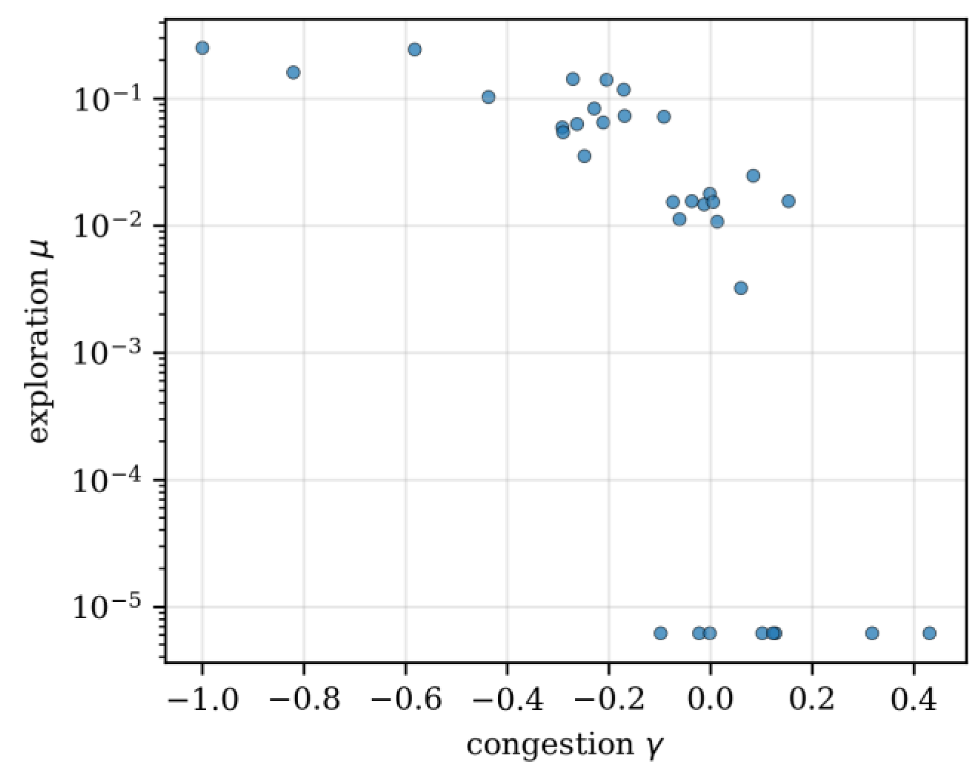
Full-sample estimates are reported for interpretation only and play no part in the forecast evaluation. On the attainment panel the congestion parameter has median -0.074 with an interquartile range from -0.249 to 0.012, and is negative for 23 of 33 countries. Negative means increasing rather than diminishing returns: the more of the population that holds a given attainment level, the more attractive that level becomes. For educational attainment this is an economically sensible reading, consistent with peer effects, network externalities in schooling, and the co-evolution of attainment with the occupational structure that rewards it. It also explains the multistability we find: eleven of the 33 attainment countries admit more than one numerically located rest point, so the same estimated dynamics imply different long-run attainment compositions from different initial conditions.
Figure 4.
Full-sample estimates of the congestion parameter and the exploration parameter, one point per country, educational attainment panel. The vertical scale is logarithmic.
Figure 4.
Full-sample estimates of the congestion parameter and the exploration parameter, one point per country, educational attainment panel. The vertical scale is logarithmic.
The waste panels behave differently. The median congestion parameter is 0.109 on the three-route panel and 0.244 on the four-route panel, positive as the congestion interpretation would predict, with negative values for 9 of 25 and 11 of 25 countries respectively. Treatment routes crowd: as more waste is directed to a route its marginal attractiveness falls, which is what capacity constraints and rising marginal disposal costs would imply.
The mutation parameter has median 0.018 on the attainment panel and 0.007 and 0.006 on the waste panels, and sits at or very near the lower bound for a substantial minority of units. In the light of Section 6.1 we decline to interpret these magnitudes behaviourally.
9. Discussion
The headline question of this paper has a negative answer. Imposing replicator-mutator structure on a compositional forecasting problem does not improve accuracy relative to generic log-ratio benchmarks. On strongly trending compositions the structural model matches the best benchmark and cannot be statistically distinguished from it; on noisy compositions neither it nor any other dynamic model beats doing nothing. Given how much the forecasting literature has had to say about the difficulty of beating simple methods, this is neither surprising nor discreditable, but it should be stated plainly rather than buried.
The more useful result is the one that emerges from the comparison of pooling regimes. Whether parameters are shared across countries matters more for accuracy than whether the model embodies an economic restriction. This has a practical implication for applied work in this area: an author who estimates an evolutionary model country by country and reports in-sample fit is making the single choice that our evidence identifies as most damaging to out-of-sample performance, and the fix costs nothing.
Three limitations qualify the findings. First, and most seriously, the mutation parameter is not separately identified from observation noise. Our Monte Carlo shows this cleanly and it is consistent with independent evidence that sampling noise in repeated cross-sections biases replicator-mutator estimates. Any structural interpretation of estimated exploration rates from data of this kind should be resisted. Second, the waste panels contain 6.1% and 6.7% zero cells, which the multiplicative replacement handles identically for all models but which inflates every log-ratio loss and may be part of why no dynamic model succeeds there. Third, the payoff specification is deliberately minimal. A richer payoff structure, with strategy-specific congestion or covariates entering the intercepts, would add parameters and, on the evidence of Section 8.2, would probably need to be pooled to be useful.
Several extensions follow directly. The divergence between win rates and mean losses in Section 8.3 invites a combination study, in which the structural model enters an ensemble rather than competing with it. The shrinkage weight could be estimated on a finer grid or replaced by a proper hierarchical estimator that shrinks each parameter separately rather than the vector as a whole; the fact that the coarse grid selects corner solutions suggests that different parameters may want different degrees of sharing. Finally, since forecasts on the simplex must cohere, the relationship between the coherence that the structural model achieves by construction and the coherence that reconciliation methods [23,24] impose after the fact is worth mapping formally.
10. Conclusions
We specified a discrete-time replicator-mutator model as a forecasting device for compositional time series, estimated it under three pooling regimes, and evaluated it against five log-ratio benchmarks on three Eurostat panels with a rolling-origin design, scale-free losses, tests of equal predictive ability, and model confidence sets.
The structural restriction does not pay for itself in accuracy. It matches the best benchmark on educational attainment, where it enters the model confidence set at the shorter horizons, and it loses to a no-change forecast on municipal waste routes, as does every other dynamic model. What does pay is parameter sharing: moving from country-specific to pooled estimation reduces scaled error by 15.3% to 27.8% across the three panels, an effect larger than the one separating the best structural model from the best benchmark. The pooled structural model also attains the highest win rate on the attainment panel and the second highest on both waste panels, indicating a loss profile different in kind from its competitors and suggesting that its proper role is as a component of a combination rather than as a stand-alone forecast.
For applied researchers using evolutionary dynamics on panels of official statistics, the operative message is that the pooling decision deserves at least as much attention as the specification of payoffs, and that out-of-sample evaluation should be the standard rather than the exception.
Funding
This research received no external funding.
Data Availability Statement
The study uses publicly available Eurostat data (online data codes edat_lfse_03 and env_wasmun). The estimation and evaluation code, the constructed panels, and all result tables are available from the author on request.
Conflicts of Interest
The author declares no conflict of interest.
Use of Generative Artificial Intelligence
Generative artificial intelligence was used for language editing and for generating the figures. The author reviewed and verified all content and takes full responsibility for the substance of the manuscript.:
References
- Aitchison, J. The statistical analysis of compositional data. J. R. Stat. Soc. Ser. B (Methodological) 1982, 44, 139–177. [Google Scholar] [CrossRef]
- Aitchison, J. The Statistical Analysis of Compositional Data; Chapman and Hall: London, UK, 1986. [Google Scholar]
- Taylor, P.D.; Jonker, L.B. Evolutionarily stable strategies and game dynamics. Math. Biosci. 1978, 40, 145–156. [Google Scholar] [CrossRef]
- Hofbauer, J.; Sigmund, K. Evolutionary Games and Population Dynamics; Cambridge University Press: Cambridge, UK, 1998. [Google Scholar]
- Weibull, J.W. Evolutionary Game Theory; MIT Press: Cambridge, MA, USA, 1995. [Google Scholar]
- Sandholm, W.H. Population Games and Evolutionary Dynamics; MIT Press: Cambridge, MA, USA, 2010. [Google Scholar]
- Schlag, K.H. Why imitate, and if so, how? A boundedly rational approach to multi-armed bandits. J. Econ. Theory 1998, 78, 130–156. [Google Scholar]
- Nowak, M.A.; Komarova, N.L.; Niyogi, P. Evolution of universal grammar. Science 2001, 291, 114–118. [Google Scholar] [CrossRef] [PubMed]
- Komarova, N.L. Replicator-mutator equation, universality property and population dynamics of learning. J. Theor. Biol. 2004, 230, 227–239. [Google Scholar] [CrossRef] [PubMed]
- Egozcue, J.J.; Pawlowsky-Glahn, V.; Mateu-Figueras, G.; Barceló-Vidal, C. Isometric logratio transformations for compositional data analysis. Math. Geol. 2003, 35, 279–300. [Google Scholar] [CrossRef]
- Pawlowsky-Glahn, V.; Egozcue, J.J.; Tolosana-Delgado, R. Modeling and Analysis of Compositional Data; Wiley: Chichester, UK, 2015. [Google Scholar]
- Kynčlová, P.; Filzmoser, P.; Hron, K. Modeling compositional time series with vector autoregressive models. J. Forecast. 2015, 34, 303–314. [Google Scholar] [CrossRef]
- Snyder, R.D.; Ord, J.K.; Koehler, A.B.; McLaren, K.R.; Beaumont, A.N. Forecasting compositional time series: A state space approach. Int. J. Forecast. 2017, 33, 502–512. [Google Scholar] [CrossRef]
- Fudenberg, D.; Levine, D.K. The Theory of Learning in Games; MIT Press: Cambridge, MA, USA, 1998. [Google Scholar]
- Young, H.P. Individual Strategy and Social Structure: An Evolutionary Theory of Institutions; Princeton University Press: Princeton, NJ, USA, 1998. [Google Scholar]
- Hyndman, R.J.; Koehler, A.B. Another look at measures of forecast accuracy. Int. J. Forecast. 2006, 22, 679–688. [Google Scholar] [CrossRef]
- Diebold, F.X.; Mariano, R.S. Comparing predictive accuracy. J. Bus. Econ. Stat. 1995, 13, 253–263. [Google Scholar] [CrossRef]
- Harvey, D.; Leybourne, S.; Newbold, P. Testing the equality of prediction mean squared errors. Int. J. Forecast. 1997, 13, 281–291. [Google Scholar] [CrossRef]
- Hansen, P.R.; Lunde, A.; Nason, J.M. The model confidence set. Econometrica 2011, 79, 453–497. [Google Scholar] [CrossRef]
- Giacomini, R.; White, H. Tests of conditional predictive ability. Econometrica 2006, 74, 1545–1578. [Google Scholar] [CrossRef]
- Elliott, G.; Timmermann, A. Economic Forecasting; Princeton University Press: Princeton, NJ, USA, 2016. [Google Scholar]
- Hyndman, R.J.; Koehler, A.B.; Ord, J.K.; Snyder, R.D. Forecasting with Exponential Smoothing: The State Space Approach; Springer: Berlin, Germany, 2008. [Google Scholar]
- Hyndman, R.J.; Ahmed, R.A.; Athanasopoulos, G.; Shang, H.L. Optimal combination forecasts for hierarchical time series. Comput. Stat. Data Anal. 2011, 55, 2579–2589. [Google Scholar] [CrossRef]
- Wickramasuriya, S.L.; Athanasopoulos, G.; Hyndman, R.J. Optimal forecast reconciliation for hierarchical and grouped time series through trace minimization. J. Am. Stat. Assoc. 2019, 114, 804–819. [Google Scholar] [CrossRef]
Table 1.
Free parameter counts by model and composition size. VAR counts include the intercept and, in the total column, the innovation covariance.
Table 1.
Free parameter counts by model and composition size. VAR counts include the intercept and, in the total column, the innovation covariance.
| Model | K = 3 (m = 2) | K = 4 (m = 3) |
|---|---|---|
| Replicator-mutator | 4 | 5 |
| Random walk with drift | 2 | 3 |
| VAR(1), conditional mean | 6 | 12 |
| VAR(1), total | 9 | 18 |
| VAR(2), total | 13 | 27 |
Table 2.
Recovery of the congestion parameter γ and the mutation parameter μ. Forty units per configuration, three parts, data generated from the structural map with logistic-normal observation noise of standard deviation σ on log-ratio coordinates.
Table 2.
Recovery of the congestion parameter γ and the mutation parameter μ. Forty units per configuration, three parts, data generated from the structural map with logistic-normal observation noise of standard deviation σ on log-ratio coordinates.
| T | σ | Bias γ | RMSE γ | Med. rel. err. γ | Bias μ | RMSE μ | Med. rel. err. μ |
|---|---|---|---|---|---|---|---|
| 15 | 0.02 | 0.008 | 0.116 | -0.003 | 0.007 | 0.023 | 0.055 |
| 15 | 0.05 | -0.770 | 4.045 | -0.015 | 0.098 | 0.231 | 0.470 |
| 15 | 0.10 | -1.061 | 3.652 | -0.086 | 0.174 | 0.311 | 1.363 |
| 25 | 0.02 | -0.107 | 0.309 | -0.013 | 0.085 | 0.185 | 0.623 |
| 25 | 0.05 | -0.033 | 0.477 | 0.006 | 0.083 | 0.188 | 0.062 |
| 25 | 0.10 | -0.881 | 2.217 | -0.193 | 0.253 | 0.360 | 7.120 |
| 40 | 0.02 | -0.062 | 0.198 | -0.003 | 0.064 | 0.144 | 0.113 |
| 40 | 0.05 | -0.180 | 1.090 | 0.002 | 0.130 | 0.247 | 0.304 |
| 40 | 0.10 | 0.174 | 0.577 | 0.125 | 0.099 | 0.179 | 2.014 |
Table 3.
Monte Carlo horse races, mean absolute scaled error averaged over horizons one to five. Panel A generates data from the structural map; Panel B from a log-ratio VAR(1) with drift.
Table 3.
Monte Carlo horse races, mean absolute scaled error averaged over horizons one to five. Panel A generates data from the structural map; Panel B from a log-ratio VAR(1) with drift.
| Model | Panel A: correct | Panel B: misspecified |
|---|---|---|
| rm_unit | 0.489 | 1.355 |
| rm_shrunk | 0.533 | 1.232 |
| rm_pool | 0.833 | 1.432 |
| Naive | 0.586 | 1.086 |
| Random walk with drift | 1.768 | 1.440 |
| ARIMA | 1.287 | 1.332 |
| Exponential smoothing | 0.689 | 1.083 |
| VAR | 0.514 | 0.977 |
Table 5.
Mean absolute scaled error by horizon, educational attainment panel. Lower is better; models ordered by the average over horizons.
Table 5.
Mean absolute scaled error by horizon, educational attainment panel. Lower is better; models ordered by the average over horizons.
| Model | h=1 | h=2 | h=3 | h=4 | h=5 | All |
|---|---|---|---|---|---|---|
| Random walk with drift | 0.579 | 0.944 | 1.221 | 1.427 | 1.635 | 1.115 |
| rm_pool | 0.590 | 0.956 | 1.218 | 1.452 | 1.666 | 1.129 |
| ARIMA | 0.604 | 0.976 | 1.260 | 1.469 | 1.678 | 1.151 |
| rm_shrunk | 0.591 | 0.970 | 1.272 | 1.528 | 1.726 | 1.167 |
| Exponential smoothing | 0.731 | 1.165 | 1.540 | 1.900 | 2.252 | 1.451 |
| rm_unit | 0.682 | 1.183 | 1.671 | 2.135 | 2.570 | 1.564 |
| VAR | 0.743 | 1.275 | 1.746 | 2.163 | 2.660 | 1.634 |
| Naive | 0.887 | 1.620 | 2.284 | 2.923 | 3.582 | 2.140 |
Table 6.
Mean absolute scaled error averaged over horizons one to five, municipal waste panels.
| Model | Waste, 3 routes | Waste, 4 routes |
|---|---|---|
| Naive | 2.417 | 2.011 |
| Exponential smoothing | 2.581 | 2.182 |
| rm_shrunk | 2.706 | 2.242 |
| Random walk with drift | 2.780 | 2.363 |
| ARIMA | 2.898 | 2.506 |
| rm_pool | 2.992 | 2.503 |
| rm_unit | 3.196 | 2.796 |
| VAR | 5.283 | 3.171 |
Table 7.
Pooling regimes versus the best benchmark, mean absolute scaled error averaged over horizons. The benchmark column gives the most accurate non-structural model on that panel. The final column is the reduction in error from moving from country-specific to the better of the two parameter-sharing regimes.
Table 7.
Pooling regimes versus the best benchmark, mean absolute scaled error averaged over horizons. The benchmark column gives the most accurate non-structural model on that panel. The final column is the reduction in error from moving from country-specific to the better of the two parameter-sharing regimes.
| Panel | rm_unit | rm_pool | rm_shrunk | Benchmark | Gain |
|---|---|---|---|---|---|
| Attainment | 1.564 | 1.129 | 1.167 | 1.115 (RW drift) | 27.8% |
| Waste, 3 routes | 3.196 | 2.992 | 2.706 | 2.417 (naive) | 15.3% |
| Waste, 4 routes | 2.796 | 2.503 | 2.242 | 2.011 (naive) | 19.8% |
Table 8.
Win rates: share of forecast events on which each model attains the lowest scaled error.
| Model | Attainment | Waste, 3 routes | Waste, 4 routes |
|---|---|---|---|
| rm_pool | 0.264 | 0.182 | 0.184 |
| Naive | 0.107 | 0.240 | 0.290 |
| ARIMA | 0.144 | 0.052 | 0.067 |
| VAR | 0.123 | 0.105 | 0.054 |
| Random walk with drift | 0.118 | 0.131 | 0.154 |
| Exponential smoothing | 0.097 | 0.164 | 0.137 |
| rm_unit | 0.091 | 0.058 | 0.041 |
| rm_shrunk | 0.056 | 0.067 | 0.073 |
Disclaimer/Publisher’s Note: The statements, opinions and data contained in all publications are solely those of the individual author(s) and contributor(s) and not of MDPI and/or the editor(s). MDPI and/or the editor(s) disclaim responsibility for any injury to people or property resulting from any ideas, methods, instructions or products referred to in the content. |
© 2026 by the authors. Licensee MDPI, Basel, Switzerland. This article is an open access article distributed under the terms and conditions of the Creative Commons Attribution (CC BY) license (http://creativecommons.org/licenses/by/4.0/).
Copyright: This open access article is published under a Creative Commons CC BY 4.0 license, which permit the free download, distribution, and reuse, provided that the author and preprint are cited in any reuse.