

Submitted:
14 August 2026
Posted:
17 August 2026
You are already at the latest version
Abstract
Protein-based biosensors exploit the extraordinary selectivity of proteins toward specific ligands—other proteins, ions, electromagnetic signals—often surpassing engineered recognition systems. Ligand binding induces structural rearrangements that alter a protein’s electrical and dielectric properties, and in electrical biosensors these changes, particularly in conductance, are what allow the target analyte to be quantified. Yet despite decades of effort, no unified strategy exists for defining and calculating protein permittivity (κ), a quantity central to interpreting such signals. Here we present a computationally inexpensive framework for evaluating protein permittivity, built on a network representation of the protein derived from its three-dimensional topology, in which each amino acid’s permittivity is assigned continuously between a dry, intrinsic value and the bulk solvent value according to its coordination number. Applied to 60 structurally diverse proteins, the model reveals a robust relationship between effective permittivity and a simple topological compactness index. As a proof of concept, we compute the electrical impedance of apo-azurin and of the protein NP_888769.1 under two electrode-contact configurations, finding a measurable, geometry-dependent response that vanishes under a uniform dielectric constant—an experimentally testable signature of internal dielectric structure that invites a re-examination of what protein permittivity experiments actually measure.
Keywords:
protein permittivity
; biosensors
; protein equivalent network
1. Introduction
Proteins are increasingly exploited in bioelectronics, most notably in biosensors [1,2,3,4,5] and optoelectronic devices [6,7]. Indeed, in vivo, proteins respond to environmental changes—pH, temperature, solute concentration, specific ligands—through conformational rearrangements [2,8,9,10] that trigger a cascade of biochemical events culminating in genuine biological “sensing,” from antigen capture to vision. In vitro biosensors harness part of this same cascade to detect the binding of a specific ligand and convert it into a chemical or physical signal [11,12]. Finally, in silico, increasingly sophisticated computational tools now support the design of biosensors and the prediction and quantification of their output signal [13,14,15,16,17].
Among the many transduction strategies available—mass, electrical, piezoelectric, chemical, optical, and so on—electrical biosensors occupy a prominent place, owing to how readily their output integrates with standard electronics. Yet several basic questions about the electrical and dielectric behavior of proteins remain open. Electrical transport is known to proceed via sequential tunneling [18,19], but the absolute resistivity of individual amino acids remains unknown [8,20], and it is not known whether—or how—this resistivity depends on the surrounding environment, unlike resistance, which is known to depend on the protein’s three-dimensional structure and to vary with conformation [8,20].
The permittivity of proteins has been calculated and measured under dry conditions [21,22,23,24], consistently yielding a narrow range, roughly 2–4. Its value in the hydrated state, presumed to be considerably larger, is still the object of active computational [25,26,27] and experimental [28] investigation. The picture is further complicated by the fact that permittivity depends strongly on temperature, degree of hydration, and protein conformation [23]. There is, however, growing consensus that permittivity should be regarded as a combination of an inner, dry-like contribution and an outer, solvent-like one, continuously distributed across the protein—that is, permittivity is intrinsically non-uniform inside a protein [23]. How large the corresponding inner and outer regions are, and how they depend on the environment, remains an open computational question [23,29]. In conclusion, calculating or measuring the permittivity of hydrated proteins remains a genuine challenge in fundamental biophysics.
Addressing permittivity is, however, also a key step in interpreting—and ultimately designing—biosensors. When measurement data are analyzed, the capacitance change associated with ligand binding is typically attributed only to macroscopic effects, i.e., changes in protein geometry [30], while the possibility of a genuine change in permittivity itself is generally overlooked. This is difficult to justify: the permittivity of a hydrated protein is known to depend substantially on the local degree of solvent exposure [23], and ligand binding necessarily changes that exposure—particularly around the binding pocket, through desolvation. It is therefore natural to reconsider the role of permittivity itself in binding processes, and hence in biosensing devices [31].
In this paper, we carry out in silico studies of the permittivity of hydrated proteins, building on a strategy introduced in [31] that complements existing analytical and computational approaches with a computationally inexpensive framework suited to the rapid analysis of large protein datasets. Our approach is grounded in well-established continuum models [23,32,33]—coarse-grained procedures that distribute permittivity continuously across the atoms or amino acids of a protein. Typically, this distribution is organized around the radius of gyration, effectively describing the protein as a shell-like structure; while this is adequate for near-spherical proteins, it becomes ineffective for markedly elongated ones [32].
Alternatively, we implement the calculation of static permittivity within the proteotronics framework [8,10], using as a structural proxy the coordination number of each amino acid, i.e., its number of nearest neighbors. This procedure has already been benchmarked against an independent approach based on the protein’s macroscopic dipole, yielding results in qualitative agreement with the sparse experimental data available [31]. In this paper, we extend the procedure to a structurally and functionally heterogeneous sample of proteins, diverse in structure and function. We find that the normalized permittivity depends only weakly on the specific interpolation function used to distribute it among amino acids—indicating that the topology of the folded protein, rather than the particular mathematical form adopted, is the dominant factor shaping the effective dielectric landscape. At the same time, it is worth focusing on functions whose parameters, once tuned, span a wide range of values, so as to capture the substantial dependence of permittivity on environmental conditions; we introduce functions whose parameters can plausibly be associated with the degree of hydration. We further show that the calculated permittivity correlates with the protein’s compactness. A non-trivial consequence of this heterogeneous dielectric model is that impedance measurements should depend on the position of the electrical contacts—a dependence that disappears under the assumption of a uniform dielectric constant, and that therefore constitutes a possible experimental signature of spatially varying protein permittivity. We test this prediction by comparing the calculated electrical impedance of apo-azurin [34] and of the novel protein NP_888769.1 [35], and find that the results indeed depend on the position of the electrical contacts, differing substantially from those obtained assuming a uniform permittivity distribution.
At present, systematic measurements of the dielectric properties of hydrated proteins remain too sparse and heterogeneous to allow quantitative calibration of any coarse-grained dielectric model. The goal of this work is therefore not quantitative—we do not aim to fix a single model or a definitive set of parameters—but rather to construct a physically motivated theoretical framework capable of generating experimentally testable predictions.
2. Materials and Methods
2.1. Materials
To test our procedure, we selected a sample of 60 proteins with significant differences in structure and function, including the same proteins in different activation states or taken from different organisms. The goal was to verify the ability of the procedure to group proteins that share similar characteristics or belong to the same family and to distinguish different configurations of the same protein. Additionally, for the same reason, proteins in the free-state or bound to other related proteins were also included. The structures were selected among the models obtained with X-ray diffraction or NMR, at high or very high resolution [36], which, at present, constitute the best representation of a hydrated protein [37]. Selection covers proteins with amino acid number,, between 55 and 828.
Among these proteins, there are 3 different models of the azurin from different species (1E65, 1AIZ, 1NZR) [34,38,39] and 4 models of lysozyme from different species (3LZT,1LZ1,162L,168L) [40,41,42,43], the bacteriorhodopsin light-driven proton pump in the light and dark-adapted configuration (2NTW,2NTU) [44], three complexes made of 2 and 3 units (2GY7, 1P9M, 2J8C) [45,46,47]; the first is angiopoietin-2 complexed with its natural receptor tyrosine kinase-2, Tie-2; the second is the cytokine IL-6 complexed with its two natural receptors, RecA and RecB; and the third is the photosynthetic reaction center with its three subunits, L, M, and H. Finally, the models of: a. IL-6 in its native state (1ALU) [48]; b. Angiopoietin-2 (Ang-2) in its native state (1Z3S) [49]; c. Receptor alpha of IL-6 in its native state (1N26) [50]; d. Ang-2 receptor, Tie-2, in its native state (2GY5) [45]. More details are reported in Table A1.
2.2. Theory & Methods
Our research is developed within the field of proteotronics, a coarse-grained description of the topological and electrical properties of proteins. This approach is time-efficient and still allows us to estimate the sensing signal provided by proteins used as active materials in biosensors [8,10,16,19,20].
We produce an equivalent of protein static relative permittivity, say k, starting from the intrinsic polarizability of each amino acid and its position in the 3D structure. In particular, each amino acid is assigned a relative permittivitywhich depends on its specific (dry) polarizability,, [31] and the coordination number, : The greater the number of neighbors, the fewer solvent molecules can reach it, or, in other words, the greater the probability that its effective permittivity remains close to its dehydrated value, and this holds regardless of the residue’s position relative to the protein’s center of mass . The coordination number is obtained by representing the protein with a network of nodes corresponding to the amino acid centroids and edges connecting close nodes. How close two nodes are considered, and the resulting network complexity, depend on the choice of a distance parameter, [8,10]. For appropriate values, the protein backbone is faithfully reproduced, and the coordination number can be used to describe the node position.
2.2.1. Models
We analyze the outputs of a pool of parametric continuous functions (models) suitable for distributing values between the intrinsic values , and the value of the solvent, , here chosen to be the typical bulk value of 80. The values of were calculated as described in [31]; by using polarizability data from [21]. Different choices [22] slightly change the value of [51]. In principle, there are no constraints on the choice of a specific function or, in other words, here we do not attempt to propose a microscopic constitutive law. Rather, we compare different smooth distributions with the aim of assessing the robustness of the framework.
We therefore consider three families of functions: polynomial, exponential, and sigmoidal. In all the following models we use at most 3 different topological variables, i.e., the maximum and minimum number of nearest neighbors, calculated for the whole protein, and the average value Finally, the independent variable is the coordination number, , normalized to its maximal value: and the average value of is taken to be the effective protein permittivity .
- Linear
- B. Polynomial
- C. Sigmoidal 1
- D. Sigmoidal 2
- E. Exponential 1
- F. Exponential
Figure 1 shows the different shapes of the listed functions. In particular, the most probable value of the protein permittivity, obtained for , decreases with the value of the free parameter () (B,C,F). On the other hand, another parameter, (C,D,E,F) tunes the sharpness of the function, not affecting the most probable value of the protein permittivity. Therefore, we propose to interpret as the hydration parameter, because for very high values of (>6) most of the residue permittivity, , is close to as in a completely hydrated protein, while, for smaller than 0.1, most of residues have values of small as in a dry condition [23]. Finally, the choice of regulates the sharpness of the function, thus setting the relative extent of the protein’s inner and outer regions [23]. Only comparison with new experimental data will be able to guarantee the validity of this interpretation and refine the parameters of the function.
3. Results
3.1. Compactness Index
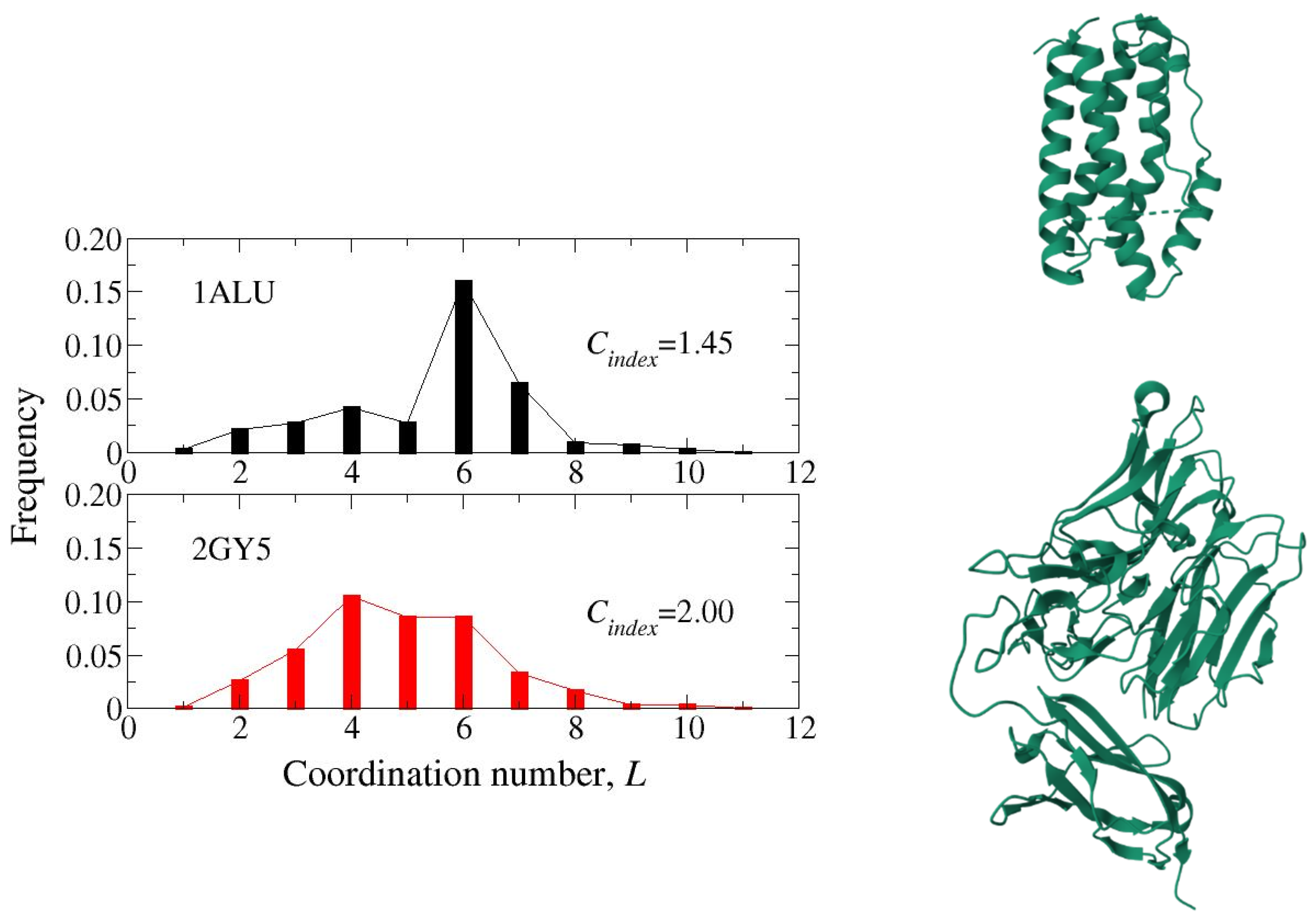
The compactness index of a protein is introduced as the ratio between the maximum value of the coordination number, say , and its average value. This quantity captures the degree of symmetry of the nearest neighbor distribution. Indeed, while represents a fairly symmetric distribution, represents a distribution dominated by high values of , corresponding to internal amino acids and therefore a very compact structure (Fig. A1). The extreme case in which the mean and maximum values of are very close, for example in coiled-coil structures, is not analyzed here. Consequently, higher values of correspond to higher values of the protein permittivity. Thus, while not an independent confirmation of the model itself, we can identify as a tool for easily interpreting the permittivity as defined here. In Figure 2 we report the permittivity values vs . Data are calculated with the 6 models, using different values of the , parameters and different values of . All the reported curves can be closely fitted by the linear relation . This relationship is very strong (correlation larger than 98%) for Models B,C with values of the parameter from small (0.25) to intermediate (2) — i.e., in our interpretation, under moderate hydration conditions. A weaker relationship is observed for Model F (correlation larger than 95%), while both in Models D and E the effective permittivity depends only weakly on . Some more details in Appendix B.
In general, it can be observed that, compared to this relationship, the interaction radius, , plays a marginal role, independently on the value of parameters; specifically, in Figure 2 data for different values of are reported for =1 in model B, for =1, =1 in models C, F, and for =1 for models D,E. Only model A shows a moderate dependence on . In this model, has also a bimodal behaviour which is presumably due to presence of the third topological parameter, .When the test function has two different parameters, and , we report data with =1 using filled symbols and data with =6 using empty symbols. These figures provide, for the sample set, a preview of the range of permittivity values, as implemented by the specific model, furthermore it easy to observe that as and/or increase, so does . Finally, in models D and E, remains limited to a very narrow range across the whole sample and model A, which has no parameters, provides quite large values of .
3.2. Role of
Although the value of does not alter the () dependence, the distribution of among the sample set depends on this parameter . Because of the scarcity of experimental data, we selected its value based on a plausibility test: In our sample, we identified several reference proteins useful to test the method. Specifically, these included three different azurins and four different lysozymes, from different biological species, a bacteriorhodopsin in different activation states, some different complexes and their constituents ( see also section 2.1).
We expect: a. very similar values for similar proteins; b. a slight difference between bacteriorhodopsin in the dark/light -adapted structure [20,44]; c. substantial differences between the compact angiopoietin-2 and the highly elongated Tie2 receptor, both composing the heterodimer 2GY7; e. Substantial differences among the constituents of the 1P9M trimer, particularly between the dense and compact interleukin IL-6 and the two receptors, which are more elongated and less compact; f. Substantial differences in the 2J8C trimer, where the two L and M chains are much more compact than the H chain.
We observed that different values of satisfy only some of these conditions and that only satisfies all of them, independently of the chosen model. This result agrees with previous investigations on the ability of a topological network to capture the main structural properties of proteins [52].
3.3. Model Selection
The comparison of the six models (A-F) is performed through the normalized permittivity, i.e., () . All models show a common trend over the set of selected proteins, while both the average , and the variance, , i.e., the relative difference among protein permittivities, are rather different (Figure 3a). Furthermore, not all proposed models allow one to adjust and freely. In particular, Model A has the maximum variance, , and quite a high value of <k>, but neither of them can be adjusted because the model has no free parameters (Figure 3a). Models D and E, which use a single parameter, q, have very small variance and a rather high value of <k>. On the other hand, by adjusting the parameters of Models B (m), and C, F (m,q), it is possible to precisely modulate the mean value of <k>.
In the 4 panels of Figure 3 we report the main results:
The normalized permittivity for the six models is reproduced in Figure 3a. Notice that while Model A exhibits the maximal variance, model D shows the minimal one.
The dependence of the permittivity average, and variance on the model parameters is shown in Figure 3b, for model B. Notice that <k> grows with while has its maximum at intermediate values of . This is in agreement with the interpretation of as a hydration indicator: for small and high values it tends to reproduce the dry and fully hydrated conditions, respectively, and both are limiting conditions in which distinguishability is lost. Similar results may be obtained also with models C and F.
An overview of absolute permittivity values is given by Figure 3c,d. Specifically, it is plotted for models A, D, E in Figure 3c and for models C,F in Figure 3d, in both cases using a wide range of parameters. Models D,E show very limited distinguishability, in particular for q=1, and cover a limited range of values of <k> . On the other hand, models C,F, as previously seen for model B, can cover a wider range of values of <k>, and have also a larger distinguishability.
In conclusion, the normalized permittivity is substantially independent of the choice of a specific model, suggesting that the proposed procedure is, in general, insensitive to the choice of the specific continuous function [31]. To simulate possible experimental data, however, some models work better than others — in particular the B, C, and F models, thanks to the wide range of permittivity values they can cover.
Therefore, we performed the following investigations using only one of them, specifically model B, which is a single-parameter (m) function. In particular, using = 0.25, we obtain, for the four lysozyme representations in our dataset, the permittivity value observed for a solvent content of 20% [23], i.e., close to 10.
3.4. Impedance Calculation
As a final step of the present investigation we numerically explore the response of a small (128 amino acids) blue-copper protein, azurin from Pseudomonas aeruginosa. This protein is taken as a model for studying electron transfer in metalloproteins [53,54,55,56,57,58] owing to its unusual copper oxidation–reduction mechanism, which is accompanied by distinctive optical properties [59]. Furthermore, its conductive response has been studied both experimentally [56,60,61] and theoretically [53,57,58], using monolayer junctions [60] as well as in single-molecule apparatus [62,63]. Here, for the sake of simplicity, we calculate the impedance of this protein in the apo form, in an ideal single-molecule apparatus [63], i.e., in a solvent such as PBS [62]. The procedure is numerically implemented in the framework of proteotronics. Specifically, after the protein equivalent network is built up, each link between a couple of nodes is dressed with the elementary impedance [8]:
where is a geometrical factor accounting for the distance and relative orientation of the corresponding amino acids, is the vacuum dielectric constant, = is the intermediate value of permittivities, are here calculated according to model B =0.25.
We perform calculations in a wide range of frequencies (0-105 rad/s), by attributing, for simplicity, a single value of resistivity to all amino acids, specifically, =6106 m, which is a typical resistivity value for non-metal bulk materials at room temperature.
The analysis is performed by solving the protein-network equivalent which is ideally contacted with an AC bias, . The flow of current inside the network, , follows, as usual, the path of minimum resistance. Finally, we calculate the protein complex impedance .
Figure 4a shows the imaginary part of impedance of apo-azurin [34] normalized to the protein resistance, . Imaginary impedance, is a very sensitive tool to test the dielectric properties of a material, since it allows fine determination of the characteristic time(s) of the process and, consequently, the protein permittivity value. It is commonly analyzed in terms of the equivalent Randles circuit [17,30,64] which mainly consists of a constant-phase element , in parallel with a resistive element, . Additional elements may be added to represent the role of the solution, the roughness of interfaces, and so on [17]. Calculations were performed using two different contact positions, in particular, up-down, as detailed in [63], using CYS3 as input and ASN42 as output, and left-right (ASN16 as input, SER66 as output). Since apo-azurin has quite a spherical shape, the global impedance is only weakly affected by the position of contacts. In both contacting configurations, the protein permittivity, say , is calculated from the maximal impedance value, using the relation , withthe protein characteristic time and the frequency producing the maximal value of the imaginary impedance, [8]. We found for values similar to, or very close to, , the average value calculated in Section 3. By contrast, we have also explored the possible effects of an elongated configuration on impedance measurements. In particular, we analyzed the features of protein NP_888769.1 from the Gram-negative bacterium Bordetella bronchoseptica (PDB code 2L25) [35]: it is similar to azurin in size (141 amino acids) and in the calculated average permittivity, , although structurally quite different [36]. In this case, changing the position of the electrical contacts produces quite different results: the left-right (PRO76-GLU141) configuration produces an impedance very close to that of an ideal resistance-capacitive (RC) parallel circuit, i.e., describes a system with a single characteristic time, while the up-down (TYR47-ALA89) configuration shows a flattened shape typical of a system of multiple characteristic times, in this case, instead of an ideal capacitor, the equivalent circuit is better described by a constant-phase element () . These results strongly suggest that the broad distribution of amino acid permittivities may produce both coherent (single-characteristic-time) and incoherent (multiple-characteristic-time) responses depending on the probe (electrical current) pathways. Finally, the up-down configuration shows a considerably higher value of permittivity. This is presumably due to the different pathways followed by the ideal current in the two configurations: the first one crosses a smaller number of boundary amino acids than the latter, thus producing a permittivity value closer to the average, while the latter highlights the boundary amino acids thus producing a higher permittivity value.
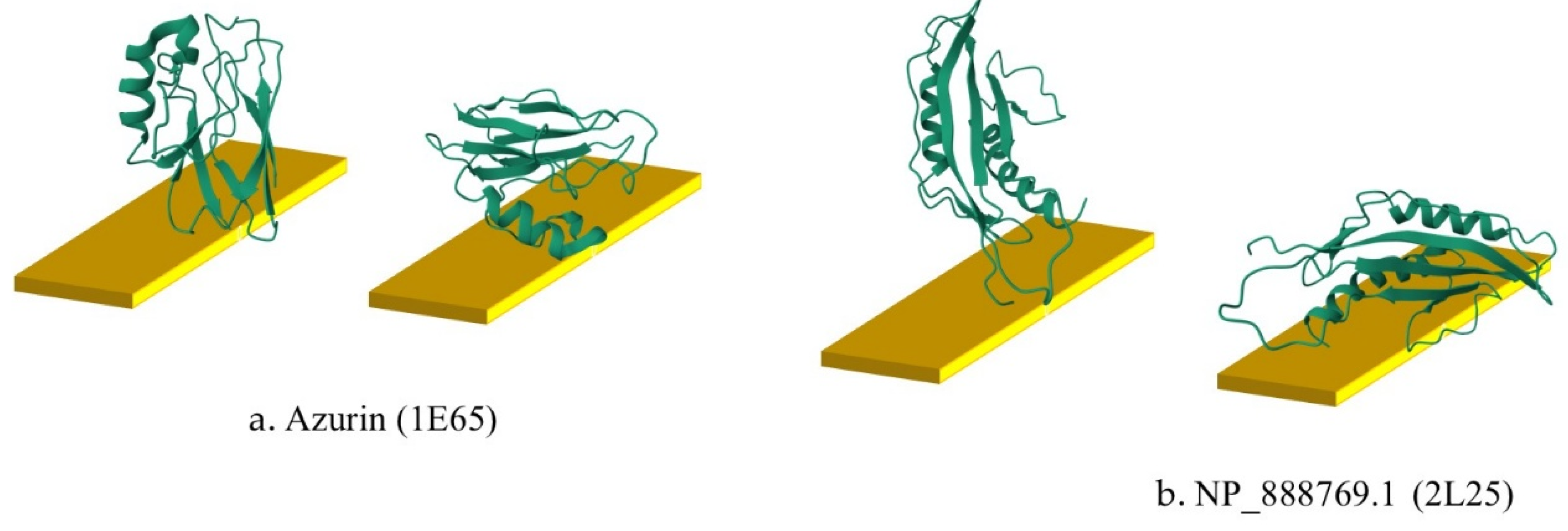
To test this hypothesis, we calculated the impedance of the two proteins in both the contacting configurations by attributing each of the amino acids the same value. The result is plotted in Figure 4c, where the 4 different impedances are calculated assuming =13 for all amino acids. In this case, all of them produce the ideal result (a single characteristic time) with the maximum equal to /2, which fully agrees with the expected response of an ideal RC parallel circuit. This difference should be used as an ultimate test to understand if the distribution of permittivity is uniform or inhomogeneous. A pictorial representation of the proteins with the two different contact positions is reported in Figure 5.
4. Discussion and Conclusions
This paper introduces a computationally efficient, topology-based framework for estimating the effective static permittivity, k, of hydrated proteins—a quantity that, despite being well defined in classical electrodynamics for bulk dielectrics, has so far resisted any unified computational treatment for proteins: existing methods are either too complex for routine use or insufficiently precise [23], and direct measurement remains experimentally challenging. The advance we propose is not a new microscopic constitutive law, but a coarse-grained, structure-only proxy—the coordination number of each amino acid—that is inexpensive to compute, requires no fitting to atomic-level chemistry, and can therefore be applied uniformly across large, structurally diverse protein datasets.
The method is implemented within proteotronics [8,10], a bottom-up procedure that derives global protein properties—such as the impedance response to an AC bias—directly from amino-acid-level features. The effective permittivity is built by continuously distributing permittivity values across the amino acids of a folded protein, using the three-dimensional structure deposited in the Protein Data Bank [36] as the reference standard. Compared with earlier implementations of the continuous-distribution approach [23,32,33], our strategy is coarse-grained at the amino-acid level rather than the atomic level, and distributes permittivity by ordering amino acids according to coordination number; at this stage it does not yet capture residue-specific chemical features (each amino acid is treated as electrically neutral [21], with no explicit propensity to interact with water). Among the possible structural descriptors of the local dielectric environment, the coordination number offers an attractive compromise between physical significance and computational efficiency: residues with many neighbors are generally less solvent-exposed and therefore experience an environment closer to the protein interior, while poorly coordinated residues are more strongly hydrated. Other descriptors, such as solvent-accessible surface area (SASA) [65,66], provide a more direct estimate of solvent exposure at the atomic level, but the coordination number is purely topological, computationally inexpensive, and robust to small structural fluctuations.
Using several smooth interpolation functions to distribute permittivity among amino acids, we obtain the effective protein permittivity, k, as the average of the individual amino-acid permittivities—the quantity we expect to be measurable at the macroscopic scale, for example via optical spectroscopy [67], though not necessarily identical to values obtained from smaller-scale experiments. A central finding of this work is that the normalized permittivity, (k − ⟨k⟩), follows a closely similar trend across the entire protein sample regardless of the specific interpolation function adopted. This indicates that the effective dielectric landscape of a protein is governed primarily by its topology, rather than by the particular mathematical form used to distribute permittivity—a degree of robustness that was not guaranteed a priori. This microscopic, topology-based estimate also compares well with an entirely independent, macroscopic approach based on the protein’s global dipole moment [31].
By contrast, the absolute value of the permittivity does depend on the specific interpolation function, which should therefore be chosen to match what is experimentally known. We selected a small number of functions whose parameters, once calibrated, can reproduce values ranging from those typical of a dehydrated protein to those of the bulk solvent. We further show that the calculated permittivity scales logarithmically with a purely topological quantity that captures the compactness of the protein, Cindex—providing a simple, structure-only estimator of a protein’s expected permittivity range ahead of any dielectric calculation.
As a concrete application, we compute the electrical imaginary impedance, ImZ, of two proteins—azurin and the novel protein NP_888769.1—a typical output of electrochemical impedance spectroscopy (EIS). These results substantiate Warshel’s point that the very definition of permittivity is subtler than it appears [68,69]: in both proteins, the permittivity extracted from the impedance calculation is close to, but distinct from, the plain average of the amino-acid permittivities, k. The discrepancy arises because solving the equivalent impedance network does not weight every amino acid’s permittivity equally, unlike a simple average: the network is built from elementary impedances, each tied to a specific amino acid’s permittivity, and the total impedance—and hence the effective permittivity it implies—depends on the current pathways selected by the network, which in turn depend on where the electrical contacts are placed. This dependence is most pronounced for a non-spherical protein such as NP_888769.1, and it constitutes a previously unrecognized experimental signature of internal dielectric heterogeneity: a measurable, contact-position-dependent response that simply disappears if permittivity is assumed uniform. This is, we believe, the paper’s most practically relevant advance: it gives experimentalists a concrete, testable way to probe whether a protein’s permittivity is uniformly or heterogeneously distributed, using nothing more than a standard EIS setup with two different contact geometries.
The present framework is intentionally coarse-grained. It neglects explicit solvent molecules, residue-specific hydrogen-bond networks, conformational dynamics, and the frequency dependence of the permittivity itself. These simplifications are what make rapid, large-scale calculations possible while still capturing the dominant topological features that shape the heterogeneous dielectric landscape; the trade-off is that the framework requires experimental input to be properly calibrated.
Ultimately, this work raises more questions than it answers: how much genuine variability in permittivity exists among proteins—modest, as suggested in [70], or substantial —and how large should the corresponding variance be in our model? What changes should be expected when structure, temperature, pressure, frequency, or hydration are varied? How should singular configurations, such as coiled coils—where the mean and maximum coordination number, , nearly coincide—be described within this framework? And how can permittivity values obtained from different types of measurement, such as EIS versus refractive index [67], be reconciled with one another? We regard these open questions not as weaknesses of the approach, but as the natural next steps that a physically grounded, computationally accessible framework now makes possible to formulate precisely.
Author Contributions
Conceptualization, E.A. and M.B.; investigation, E.A.; writing—original draft preparation, E.A.; writing—review and editing, M.B.; visualization, M.B. All authors have read and agreed to the published version of the manuscript.
Funding
This paper has been partially funded by the Italian MUR project GINEVRA, prot. 2022BZYBWM. This work is supported by the INFN grant GAST.
Institutional Review Board Statement
Not applicable.
Informed Consent Statement
Not applicable.
Data Availability Statement
Data are available to interested researchers upon request.
Conflicts of Interest
The authors declare no conflicts of interest.
Appendix A
Data Set
The complete dataset of selected proteins is reported in Table A1.

Table A1.
The complete protein dataset. The Table shows: the protein’s PDB code [36] , the number of amino acids,, the compactness index calculated for , the equivalent permittivity, , calculated within Model B, =0.25,.
Table A1.
The complete protein dataset. The Table shows: the protein’s PDB code [36] , the number of amino acids,, the compactness index calculated for , the equivalent permittivity, , calculated within Model B, =0.25,.
| Protein ID# | Type |
Reference | |||
|---|---|---|---|---|---|
| 1CNR | Crambin | 46 | 1.9 | 13 | [71] |
| 1C09 | Rubredoxin | 53 | 1.9 | 13 | [72] |
| 1C9O | Cold Shock Protein |
66 | 1.6 | 10 | [73] |
| 1UBQ | Ubiquitin | 76 | 1.8 | 12 | [74] |
| 1UZ3 | Emsy Protein |
102 | 1.8 | 12 | [75] |
| 1BRK | Barnase | 108 | 1.8 | 12 | [76] |
| 1BKR | Calponin | 108 | 1.6 | 10 | [77] |
| 1FS3 | Pancreatic ribonuclease A | 124 | 1.7 | 11 | [78] |
| 1E65 | Azurin (apo) –P.aeruginosa- | 128 | 1.9 | 13 | [34] |
| 1NZR | Azurin mutant –P.aeruginosa- | 129 | 1.9 | 13 | [39] |
| 3LZT | Lysozime -gallus gallus- | 129 | 1.7 | 11 | [40] |
| 1AIZ | Azurin(apo) –A.denitrificans- | 130 | 1.9 | 12 | [38] |
| 1LZ1 | Lysozime –homo sapiens- | 130 | 1.8 | 12 | [41] |
| 1AU7 | PIT-1 mutant | 130 | 1.9 | 12 | [79] |
| 2L25 | NP_888769.1 | 141 | 1.9 | 13 | [35] |
| 1B0B | Haemoglobin –p.pectinatus- | 141 | 1.7 | 10 | [80] |
| 1XJS | IscU | 147 | 1.9 | 13 | [81] |
| 1CFC | Calcium-free Calmodulin | 148 | 1.7 | 11 | [82] |
| 1WLA | Myoglobin –E.ferus- | 153 | 1.7 | 10 | [83] |
| 1MBN | Myoglobin –p.macrocephalus- | 153 | 1.7 | 10 | [84] |
| 1ALU | Cytokine IL-6 | 157 | 1.8 | 12 | [48] |
| 162L | Phage T4 Lysozyme | 162 | 1.7 | 11 | [42] |
| 1P9M_B | Cytokine IL-6 in complex | 163 | 1.8 | 12 | [46] |
| 168L | T4-Lysozyme | 164 | 1.5 | 9 | [43] |
| 3NP1 | Nitrophorine | 184 | 1.8 | 11 | [85] |
| 8ZF2 | HapR | 189 | 1.7 | 11 | [86] |
| 1P9M_C | Gp-130 in complex | 201 | 1.9 | 13 | [46] |
| 2GY7_ANG2 | Angiopoietin-2 in complex | 216 | 1.7 | 11 | [45] |
| 1Z3S | Angiopoietin-2, Ang-2 | 216 | 1.8 | 12 | [49] |
| 2NTU | Bacteriorhodopsin/dark | 222 | 1.9 | 13 | [44] |
| 2NTW | Bacteriorhodopsin/light | 222 | 1.8 | 11 | [44] |
| 2J8C_H | Reaction center_chain H | 240 | 2.2 | 16 | [47] |
| 1N2Z | BtuF | 244 | 1.8 | 12 | [87] |
| 1P9L | Dihydrodipicolinate reductase | 245 | 1.9 | 13 | [88] |
| 1H6G | Alpha-catenin (M-fragment) | 248 | 1.8 | 11 | [89] |
| 1AU7 | Pit-1 mutant | 258 | 1.8 | 11 | [79] |
| 2J8C_L | Reaction center_chain L | 281 | 1.9 | 13 | [47] |
| 4FZA_B | MST4 in complex | 282 | 1.9 | 13 | [90] |
| 1P9M_A | IL-6 -receptor in complex | 298 | 1.9 | 13 | [46] |
| 1N26 | IL-6 -receptor | 299 | 1.9 | 13 | [50] |
| 2J8C_M | Reaction center_chain M | 302 | 1.8 | 12 | [47] |
| 1ABE | L-arabinose binding protein | 305 | 1.9 | 13 | [91] |
| 1GKZ | Bckd Kinase | 316 | 1.8 | 12 | [92] |
| 4FZA_A | MO25 in complex | 324 | 1.8 | 11 | [90] |
| 1U19 | Bovine rhodopsin | 348 | 1.8 | 12 | [93] |
| 1P9M_BC | IL-6/gp-130 complex | 364 | 2.0 | 14 | [46] |
| 2GY5 | Tyrosin kinase, Tie-2 | 423 | 2.2 | 16 | [45] |
| 2GY7_TIE2 | Tyrosin kinase, Tie-2 in complex | 423 | 2.0 | 14 | [45] |
| 3EHS | CRFR1 | 452 | 1.8 | 11 | [94] |
| 13ZS | 3Dpol RNA | 457 | 1.8 | 11 | [95] |
| 3EHT | CRFR1 in complex | 462 | 2.1 | 14 | [94] |
| 1P9M_AB | IL-6 -receptor/IL-6 complex | 461 | 2.0 | 14 | [46] |
| 4ZJ8 | Human orexin receptor, OX1 | 503 | 1.7 | 11 | [96] |
| 2ACE | Acetilcholinesterase | 527 | 2.1 | 15 | [97] |
| 7FIJ | glycoprotein hormone receptor signalling complexes | 561 | 1.7 | 11 | [98] |
| 2J8C_LM | Reaction center_chain LM | 583 | 1.8 | 12 | [47] |
| 2GY7 | Ang-2/Tie-2 in complex | 639 | 2.0 | 13 | [45] |
| 1P9M | IL-6-receptor/IL-6/gp-130 complex | 662 | 2.0 | 14 | [46] |
| 2J8C | Reaction center, pH 8 | 823 | 1.9 | 12 | [47] |
| 2UXJ | Reaction center, pH 10 | 823 | 1.9 | 12 | [47] |
Figure A1 shows two examples of proteins with very different values , specifically, the IL-6 cytokine (1ALU), a 4-helix bundle protein, and the angiopoietin 2 receptor, Tie-2 (2GY5), a complex structure made of three immunoglobulin domains.
For 1ALU, the link distribution is rather narrow, bell-shaped, with a maximum at =6Å , thus demonstrating a compact and regular structure with few outliers. On the other hand, the second distribution is very uniform with many more nodes having limited number of links. Calculations were performed using =6Å.
Figure A1.
Link distribution for interleukin IL-6 (1ALU) and tyrosine kinase Tie-2 (2GY5).
Appendix B
The data resulting from fitting the permittivity as a function of the compactness index, , are shown in Tables B1–B6.
The interpolating function is:
with fitting parameters, .
The correlation values are for the raw data of the entire dataset, organized per model and parameter values.
Table B1.
Fitting parameters of Equation B1 for Model B,
| m | a, b |
Correlation coefficient |
| 6 | 59, 25 | 0.84 |
| 3 | 38, 42 | 0.962 |
| 2 | 25, 47 | 0.987 |
| 1 | 10, 43 | 0.998 |
| 0.5 | 3.6, 30 | 0.998 |
| 0.25 | 1.2, 18 | 0.996 |
Table B2.
Fitting parameters of Equation B1 for Model B,
| RC () | a, b |
Correlation coefficient |
| 5 | 12, 39 | 0.995 |
| 6 | 10, 43 | 0.998 |
| 7 | 8, 47 | 0.999 |
| 8 | 9, 45 | 0,999 |
| 9 | 9, 46 | 0.999 |
| 12 | 9, 45 | 0.999 |
Table B3.
Fitting parameters of Equation B1 for Model C,
| m | q | a, b |
Correlation coefficient |
| 6 | 1 | 31, 12 | 0.94 |
| 1 | 1 | 5.7, 23 | 0.99 |
| 0.5 | 1 | 2, 16 | 0.98 |
| 1 | 6 | 7, 26 | 0.91 |
| 0.5 | 6 | 2.5, 19 | 0.92 |
Table B4.
Fitting parameters of Equation B1 for Model C,
| RC () | a, b | Correlation coefficient |
| 5 | 12, 39 | 0.995 |
| 6 | 10, 43 | 0.998 |
| 7 | 8,47 | 0.999 |
| 8 | 9, 45 | 0.999 |
| 9 | 9, 46 | 0.999 |
| 12 | 9, 45 | 0.999 |
Table B5.
Fitting parameters of Equation B1 for Model D,
| Q | a, b | Correlation coefficient |
| 6 | 39, 4.7 | 0.40 |
| 1 | 40, 1.4 | 0.52 |
Table B6.
Fitting parameters of Equation B1 for Model F, .
| m | q | a, b | Correlation coefficient |
| 6 | 1 | 23, 9 | 0.966 |
| 1 | 1 | 5, 18 | 0.963 |
| 0.5 | 1 | 2, 13 | 0.95 |
| 1 | 6 | 5, 23 | 0.83 |
| 0.5 | 6 | 2, 17 | 0.85 |
B2. The Role of
As announced in Section 3.2, the normalized permittivity depends weakly on the interaction radius, . In the following figures we report the equivalent of Figure 3a, here calculated for =7Å and = 12 Å.
Figure B1.
Normalized permittivity calculated for the dataset.The normalized permittivity is plotted for the selected proteins permittivity using the six models (A-F); calculation are performed using , .
Figure B1.
Normalized permittivity calculated for the dataset.The normalized permittivity is plotted for the selected proteins permittivity using the six models (A-F); calculation are performed using , .
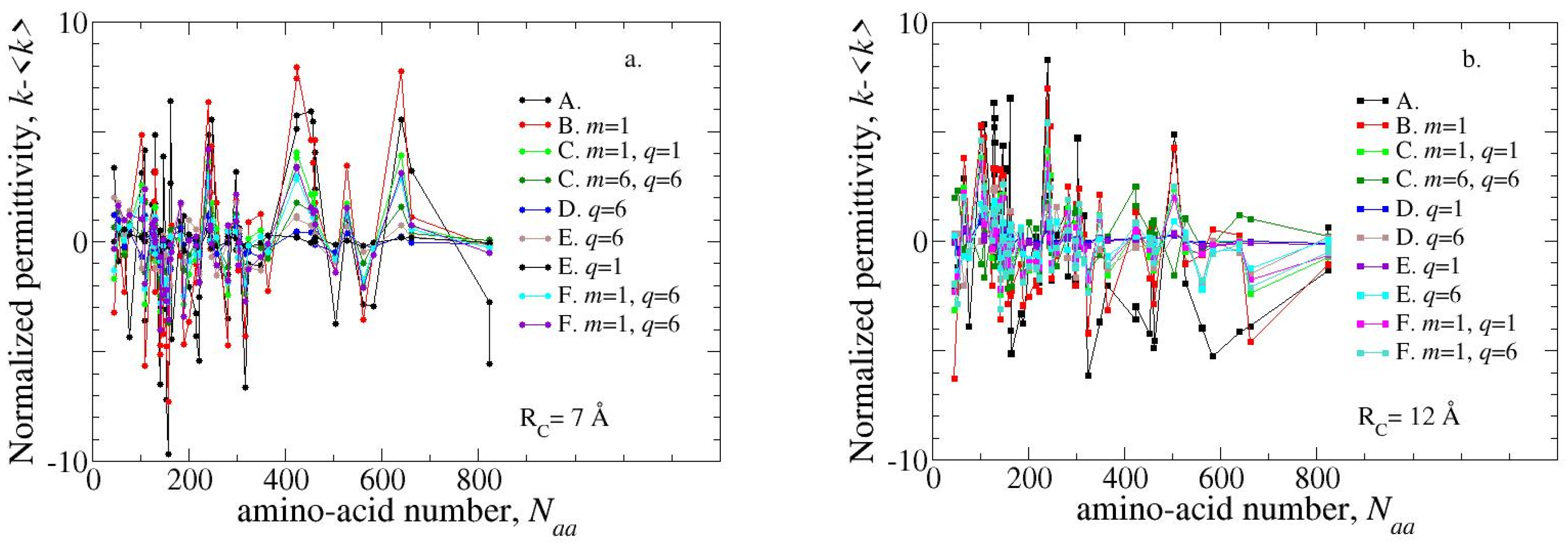
It can be noted that, although each provides its own specific profile, presents a trend very similar to that of In all the cases analyzed, the normalized permittivity has a trend that is little dependent on the model, regardless of the value of .
References
- Misawa, N.; Osaki, T.; Takeuchi, S. Membrane protein-based biosensors. J. R Soc. Interface 2018, 15, 20170952. [Google Scholar] [CrossRef]
- Alexandrov, K.; Vickers, C. E. In vivo protein-based biosensors: seeing metabolism in real time. Trends Biotechnol. 2023, 41, 19–26. [Google Scholar] [CrossRef]
- Chaisupa, P.; Wright, R. C. State-of-the-art in engineering small molecule biosensors and their applications in metabolic engineering. SLAS Technol. 2024, 29, 100113. [Google Scholar] [CrossRef]
- Torculas, M.; Medina, J.; Xue, W.; Hu, X. Protein-based bioelectronics. ACS Biomater. Sci. Eng. 2016, 2, 1211–1223. [Google Scholar] [CrossRef]
- Bostick, C. D.; Mukhopadhyay, S.; Pecht, I.; Sheves, M.; Cahen, D.; Lederman, D. Protein bioelectronics: A review of what we do and do not know. Rep. Prog. Phys. 2018, 81, 026601. [Google Scholar] [CrossRef]
- Jiang, T.; Zeng, B. F.; Zhang, B.; Tang, L. Single-molecular protein-based bioelectronics via electronic transport: fundamentals, devices and applications. Chem. Soc. Rev. 2023, 52, 5968–6002. [Google Scholar]
- Xu, S.; Momin, M.; Ahmed, S.; Hossain, A.; Veeramuthu, L.; Pandiyan, A.; …; Zhou, T. Illuminating the brain: advances and perspectives in optoelectronics for neural activity monitoring and modulation. Adv. Mater. 2023, 35, 2303267. [Google Scholar] [CrossRef]
- Alfinito, E.; Pousset, J.; Reggiani, L. Proteotronics: development of protein-based electronics; Publisher: CRC Press: Boca-Raton, Florida, 2015. [Google Scholar]
- Alfinito, E.; Beccaria, M.; Ciccarese, M. Biosensing cytokine IL-6: a comparative analysis of natural and synthetic receptors. Biosensors 2020, 10, 106. [Google Scholar] [CrossRef]
- Alfinito, E.; Pousset, J.; Reggiani, L. PROTEOTRONICS: The emerging science of protein-based electronic devices. In J Phys Conf Ser; IOP Publishing, 2015; Vol. 647, No. 1, p. 012002. [Google Scholar]
- Khizar, S.; Zine, N.; Errachid, A.; Elaissari, A. Proteins based nanoparticles for drug delivery: critical review. Curr. Opin. Colloid Interface Sci. 2025, 101971. [Google Scholar] [CrossRef]
- Vidic, J.; Manzano, M.; Chang, C. M.; Jaffrezic-Renault, N. Advanced biosensors for detection of pathogens related to livestock and poultry. Vet. Res. 2017, 48, 11. [Google Scholar] [CrossRef]
- Penchovsky, R. Computational design of allosteric ribozymes as molecular biosensors. Biotechnol. Adv. 2014, 32, 1015–1027. [Google Scholar] [CrossRef]
- Khoshbin, Z.; Housaindokht, M. R.; Izadyar, M.; Bozorgmehr, M. R.; Verdian, A. Recent advances in computational methods for biosensor design. Biotechnol. Bioeng. 2021, 118, 555–578. [Google Scholar] [CrossRef]
- Jesky, R. G.; Lo, L. H.; Siu, R. H.; Tanner, J. A. Designing the Future of Biosensing: Advances in Aptamer Discovery, Computational Modeling, and Diagnostic Applications. Biosensors 2025, 15, 637. [Google Scholar] [CrossRef]
- Cataldo, R.; Ciriaco, F.; Alfinito, E. A validation strategy for in silico generated aptamers. Comput. Biol. Chem. 2018, 77, 123–130. [Google Scholar] [CrossRef]
- Guascito, M. R.; Alfinito, E.; Cataldo, R.; Giotta, L. Tips for a (simple) interpretation of the impedance response of an electrochemical cell. IEEE Sens. J. 2019, 19, 11318–11322. [Google Scholar] [CrossRef]
- Baranovski, S. (Ed.) Charge transport in disordered solids with applications in electronics; John Wiley & Sons Ltd.: The Atrium, Southern Gate, Chichester, West Sussex, PO198SQ, England, 2006. [Google Scholar]
- Alfinito, E.; Reggiani, L. Evidence of Gumbel distributions of conductance fluctuations in bacteriorhodopsin thin films. J. Phys. Cond. Mat. 2013, 25, 375103. [Google Scholar] [CrossRef]
- Alfinito, E.; Reggiani, L. Mechanisms responsible for the photocurrent in bacteriorhodopsin. Phys. Rev. E 2015, 91, 032702. [Google Scholar] [CrossRef]
- Song, X. An inhomogeneous model of protein dielectric properties: Intrinsic polarizabilities of amino acids. J. Chem. Phys. 2002, 116, 9359–9363. [Google Scholar] [CrossRef]
- Amin, M.; Küpper, J. Variations in proteins dielectric constants. ChemistryOpen 2020, 9, 691–694. [Google Scholar] [CrossRef]
- Simonson, T. Electrostatics and dynamics of proteins. Rep. Progr Phys. 2003, 66, 737–787. [Google Scholar] [CrossRef]
- Bibi, F.; Villain, M.; Guillaume, C.; Sorli, B.; Gontard, N. A review: Origins of the dielectric properties of proteins and potential development as bio-sensors. Sensors 2016, 16, 1232. [Google Scholar] [CrossRef]
- Heyden, M.; Matyushov, D. V. Dielectrophoresis of proteins in solution. J. Phys. Chem. B 2020, 124, 11634–11647. [Google Scholar] [CrossRef]
- Wang, L.; Zhang, Z.; Rocchia, W.; Alexov, E. Using DelPhi capabilities to mimic protein’s conformational reorganization with amino acid specific dielectric constants. Commun. Comput. Phys. 2013, 13, 13–30. [Google Scholar] [CrossRef]
- Rocchia, W.; Neshich, G. Electrostatic potential calculation for biomolecules: creating a database of pre-calculated values reported on a per residue basis for all PDB protein structures. Genet Mol. Res. 2007, 6, 923–936. [Google Scholar]
- Kukic, P.; Farrell, D.; McIntosh, L. P.; García-Moreno E, B.; Jensen, K. S.; Toleikis, Z.; …; Nielsen, J. E. Protein dielectric constants determined from NMR chemical shift perturbations. J. Am. Chem. Soc. 2013, 135, 16968–16976. [Google Scholar] [CrossRef]
- Simonson, T.; Brooks, C. L. Charge screening and the dielectric constant of proteins: insights from molecular dynamics. J. Am. Chem. Soc. 1996, 118, 8452–8458. [Google Scholar] [CrossRef]
- Bard, A. J.; Faulkner, L. R.; White, H. S. Electrochemical methods: fundamentals and applications; John Wiley & Sons, 2022. [Google Scholar]
- Alfinito, E.; Beccaria, M. Dielectric response in proteins: the proteotronics approach. Transp. Phenom. 2026, 1, 20260030. [Google Scholar] [CrossRef]
- Li, L.; Li, C.; Zhang, Z.; Alexov, E. On the dielectric “constant” of proteins: smooth dielectric function for macromolecular modeling and its implementation in DelPhi. J. Chem. Theoy Comput 2013, 9, 2126–2136. [Google Scholar] [CrossRef]
- Grant, J. A.; Pickup, B. T.; Nicholls, A. A smooth permittivity function for Poisson–Boltzmann solvation methods. J. Comput. Chem. 2001, 22, 608–640. [Google Scholar] [CrossRef]
- Nar, H.; Messerschmidt, A.; Huber, R.; Van de Kamp, M.; Canters, G. W. Crystal structure of Pseudomonas aeruginosa apo-azurin at 1.85 Å resolution. FEBS Lett. 1992, 306(2-3), 119–124. [Google Scholar] [CrossRef]
- Wahab, A. T.; Serrano, P.; Geralt, M.; Wüthrich, K. NMR structure of the Bordetella bronchiseptica protein NP_888769. 1 establishes a new phage-related protein family PF13554. Protein Sci. 2011, 20, 1137–1144. [Google Scholar] [CrossRef]
- Berman, H. M.; Battistuz, T.; Bhat, T. N.; Bluhm, W. F.; Bourne, P. E.; Burkhardt, K.; …; Zardecki, C. The protein data bank. Biol. Crystallogr. 2002, 58, 899–907. [Google Scholar] [CrossRef]
- Maveyraud, L.; Mourey, L. Protein X-ray crystallography and drug discovery. Molecules 2020, 25, 1030. [Google Scholar] [CrossRef]
- Shepard, W. E. B.; Kingston, R. L.; Anderson, B. F.; Baker, E. N. Structure of apo-azurin from Alcaligenes denitrificans at 1.8 Å resolution. Biol. Cryst. 1993, 49, 331–343. [Google Scholar] [CrossRef]
- Tsai, L. C.; Sjölin, L.; Langer, V.; Bonander, N.; Karlsson, B.G.; Vänngård, T.; Hammann, C.; Nar, H. Structure of the azurin mutant nickel–Trp48Met from Pseudomonas aeruginosa at 2.2 Å resolution. Biol. Cryst. 1995, 51, 711–717. [Google Scholar] [CrossRef]
- Walsh, M. A.; Schneider, T. R.; Sieker, L. C.; Dauter, Z.; Lamzin, V. S.; Wilson, K. S. Refinement of triclinic hen egg-white lysozyme at atomic resolution. Biol. Cryst. 1998, 54, 522–546. [Google Scholar] [CrossRef]
- Artymiuk, P. J.; Blake, C. C. F. Refinement of human lysozyme at 1.5 Å resolution analysis of non-bonded and hydrogen-bond interactions. J. Mol. Bio 1981, 152, 737–762. [Google Scholar] [CrossRef]
- Blaber, M.; Baase, W. A.; Gassner, N.; Matthews, B. W. Alanine scanning mutagenesis of the α-helix 115-123 of phage T4 lysozyme: effects on structure, stability and the binding of solvent. J. Mol. Bio 1995, 246, 317–330. [Google Scholar] [CrossRef]
- Zhang, X. J.; Wozniak, J. A.; Matthews, B. W. Protein flexibility and adaptability seen in 25 crystal forms of T4 lysozyme. J. Mol. Bio 1995, 250, 527–552. [Google Scholar] [CrossRef]
- Lanyi, J. K.; Schobert, B. Structural changes in the L photointermediate of bacteriorhodopsin. J. Mol. Bio 2007, 365, 1379–1392. [Google Scholar] [CrossRef]
- Barton, W. A.; Tzvetkova-Robev, D.; Miranda, E.P.; Kolev, M.V.; Rajashankar, K.R.; Himanen, J.P.; Nikolov, D.B. Crystal structures of the Tie2 receptor ectodomain and the angiopoietin-2–Tie2 complex. Nat. Struct. Mol. Biol. 2006, 13, 524–532. [Google Scholar] [CrossRef]
- Boulanger, M. J.; Chow, D. C.; Brevnova, E. E.; Garcia, K. C. Hexameric structure and assembly of the interleukin-6/IL-6 α-receptor/gp130 complex. Science 2003, 300, 2101–2104. [Google Scholar] [CrossRef]
- Koepke, J.; Krammer, E. M.; Klingen, A. R.; Sebban, P.; Ullmann, G. M.; Fritzsch, G. pH modulates the quinone position in the photosynthetic reaction center from Rhodobacter sphaeroides in the neutral and charge separated states. J. Mol. Bio 2007, 371, 396–409. [Google Scholar] [CrossRef]
- Somers, W.; Stahl, M.; Seehra, J. S. 1.9 Å crystal structure of interleukin 6: implications for a novel mode of receptor dimerization and signaling. EMBO J. 1997, 16, 989–997. [Google Scholar] [CrossRef]
- Barton, W. A.; Tzvetkova, D.; Nikolov, D. B. Structure of the angiopoietin-2 receptor binding domain and identification of surfaces involved in Tie2 recognition. Structure 2005, 13, 825–832. [Google Scholar] [CrossRef]
- Varghese, J. N.; Moritz, R. L.; Lou, M. Z.; Van Donkelaar, A.; Ji, H.; Ivancic, N.; …; Simpson, R. J. Structure of the extracellular domains of the human interleukin-6 receptor α-chain. PNAS 2002, 99, 15959–15964. [Google Scholar] [CrossRef]
- Alfinito; E. Beccaria, M. Permittivity in protein-based sensors: the role of topology. Prep.
- Pollastri, G.; Baldi, P.; Fariselli, P.; Casadio, R. Prediction of coordination number and relative solvent accessibility in proteins. Proteins Struct. Funct. Bioinform. 2002, 47, 142–153. [Google Scholar] [CrossRef]
- Bizzarri, A. R.; Baldacchini, C.; Cannistraro, S. Structure, dynamics, and electron transfer of azurin bound to a gold electrode. Langmuir 2017, 33, 9190–9200. [Google Scholar] [CrossRef]
- Kayser, B.; Fereiro, J. A.; Guo, C.; Cohen, S. R.; Sheves, M.; Pecht, I.; Cahen, D. Transistor configuration yields energy level control in protein-based junctions. Nanoscale 2018, 10, 21712–21720. [Google Scholar] [CrossRef]
- Tuzhilkin, R.; Ondruška, V.; Šulc, M. Azurin: a model to study a metal coordination sphere or electron transfer in metalloproteins. Int. J. Mol. Sci. 2025, 26, 4125. [Google Scholar] [CrossRef]
- Maruccio, G.; Biasco, A.; Visconti, P.; Bramanti, A.; Pompa, P. P.; Calabi, F.; …; Canters, G. W. Towards protein field-effect transistors: report and model of a prototype. Adv. Mater. 2005, 17, 816–822. [Google Scholar] [CrossRef]
- Valianti, S.; Cuevas, J. C.; Skourtis, S. S. Charge-transport mechanisms in azurin-based monolayer junctions. J. Phys. Chem. C 2019, 123, 5907–5922. [Google Scholar] [CrossRef]
- Roldán-Piñero, C.; Romero-Muñiz, C.; Díez-Pérez, I.; Vilhena, J. G.; Pérez, R.; Cuevas, J. C.; Zotti, L. A. Efficient electron hopping transport through azurin-based junctions. J. Phys. Chem. Lett. 2023, 14, 11242. [Google Scholar] [CrossRef]
- Bizzarri, A. R.; Andolfi, L.; Taranta, M.; Cannistraro, S. Optical and electronic coupling of the redox copper Azurin on ITO-coated quartz substrate. Biosens. Bioelectron. 2008, 24, 204–209. [Google Scholar] [CrossRef]
- Bordi, F.; Prato, M.; Cavalleri, O.; Cametti, C.; Canepa, M.; Gliozzi, A. Azurin self-assembled monolayers characterized by coupling electrical impedance spectroscopy and spectroscopic ellipsometry. J. Phys. Chem. B 2004, 108, 20263–20272. [Google Scholar] [CrossRef]
- Li, P. A.; Bera, S.; Kumar-Saxena, S.; Pecht, I.; Sheves, M.; Cahen, D.; Selzer, Y. Electron transport through two interacting channels in Azurin-based solid-state junctions. PNAS 2024, 121, e2405156121. [Google Scholar] [CrossRef]
- Taranta, M.; Bizzarri, A. R.; Cannistraro, S. Probing the interaction between p53 and the bacterial protein azurin by single molecule force spectroscopy. J. Mol. Recognit. An. Interdiscip. J. 2008, 21, 63–70. [Google Scholar] [CrossRef]
- Fereiro, J. A.; Bendikov, T.; Pecht, I.; Sheves, M.; Cahen, D. Protein binding and orientation matter: Bias-induced conductance switching in a mutated azurin junction. J. Am. Chem. Soc. 2020, 142, 19217. [Google Scholar] [CrossRef]
- Orazem, M. E.; Pébère, N.; Tribollet, B. Enhanced graphical representation of electrochemical impedance data. J. Electrochem. Soc. 2006, 153, B129–B136. [Google Scholar] [CrossRef]
- Durham, E.; Dorr, B.; Woetzel, N.; Staritzbichler, R.; Meiler, J. Solvent accessible surface area approximations for rapid and accurate protein structure prediction. J. Mol. Model 2009, 15, 1093–1108. [Google Scholar] [CrossRef]
- Ausaf Ali, S.; Imtaiyaz Hassan, M.; Islam, A.; Ahmad, F. A review of methods available to estimate solvent-accessible surface areas of soluble proteins in the folded and unfolded states. Curr. Protein Pept. Sci. 2014, 15, 456–476. [Google Scholar] [CrossRef]
- Vinh, N. Q.; Allen, S. J.; Plaxco, K. W. Dielectric spectroscopy of proteins as a quantitative experimental test of computational models of their low-frequency harmonic motions. J. Am. Chem. Soc. 2011, 133, 8942–8947. [Google Scholar] [CrossRef]
- Warshel, A.; Sharma, P. K.; Kato, M.; Parson, W. W. Modeling electrostatic effects in proteins. Biochim. Et. Biophys. Acta (BBA) -Proteins Proteom. 2006, 1764, 1647–1676. [Google Scholar] [CrossRef]
- Schutz, C. N.; Warshel, A. What are the dielectric “constants” of proteins and how to validate electrostatic models? Proteins Struct. Funct. Bioinform. 2001, 44, 400–417. [Google Scholar] [CrossRef]
- Felder, C. E.; Prilusky, J.; Silman, I.; Sussman, J. L. A server and database for dipole moments of proteins. Nucleic Acids Res. 2007, 35, W512–W521. [Google Scholar] [CrossRef]
- Yamano, A.; Teeter, M. M. Correlated disorder of the pure Pro22/Leu25 form of crambin at 150 K refined to 1.05-A resolution. J. Bio Chem. 1994, 269, 13956–13965. [Google Scholar] [CrossRef]
- Eidsness, M. K.; Burden, A. E.; Richie, K. A.; Kurtz, D. M.; Scott, R. A.; Smith, E. T.; …; Kang, C. -Modulation of the redox potential of the [Fe (SCys) 4] site in rubredoxin by the orientation of a peptide dipole. Biochemistry 1999, 38, 14803–14809. [Google Scholar] [CrossRef]
- Mueller, U.; Perl, D.; Schmid, F. X.; Heinemann, U. Thermal stability and atomic-resolution crystal structure of the Bacillus caldolyticus cold shock protein. J. Mol. Bio 2000, 297, 975–988. [Google Scholar] [CrossRef]
- Vijay-Kumar, S.; Bugg, C. E.; Cook, W. J. Structure of ubiquitin refined at 1.8 Å resolution. J. Mol. Bio 1987, 194, 531–544. [Google Scholar] [CrossRef]
- Chavali, G. B.; Ekblad, C. M.; Basu, B. P.; Brissett, N. C.; Veprintsev, D.; Hughes-Davies, L.; …; Doherty, A. J. Crystal structure of the ENT domain of human EMSY. J. Mol. Bio 2005, 350, 964–973. [Google Scholar] [CrossRef]
- Buckle, A. M.; Cramer, P.; Fersht, A. R. Structural and energetic responses to cavity-creating mutations in hydrophobic cores: observation of a buried water molecule and the hydrophilic nature of such hydrophobic cavities. Biochemistry 1996, 35, 4298–4305. [Google Scholar] [CrossRef]
- Bañuelos, S.; Saraste, M.; Carugo, K. D. Structural comparisons of calponin homology domains: implications for actin binding. Structure 1998, 6, 1419–1431. [Google Scholar] [CrossRef]
- Chatani, E.; Hayashi, R.; Moriyama, H.; Ueki, T. Conformational strictness required for maximum activity and stability of bovine pancreatic ribonuclease A as revealed by crystallographic study of three Phe120 mutants at 1.4 Å resolution. Protein Sci. 2002, 11, 72–81. [Google Scholar] [CrossRef]
- Jacobson, E. M.; Li, P.; Leon-del-Rio, A.; Rosenfeld, M. G.; Aggarwal, A. K. Structure of Pit-1 POU domain bound to DNA as a dimer: unexpected arrangement and flexibility. Genes Dev. 1997, 11, 198–212. [Google Scholar] [CrossRef]
- Bolognesi, M.; Rosano, C.; Losso, R.; Borassi, A.; Rizzi, M.; Wittenberg, J. B.; …; Ascenzi, P. Cyanide binding to Lucina pectinata hemoglobin I and to sperm whale myoglobin: an x-ray crystallographic study. Biophys. J. 1999, 77, 1093–1099. [Google Scholar] [CrossRef]
- Ramelot, T. A.; Cort, J. R.; Goldsmith-Fischman, S.; Kornhaber, G. J.; Xiao, R.; Shastry, R.; …; Kennedy, M. A. Solution NMR structure of the iron–sulfur cluster assembly protein U (IscU) with zinc bound at the active site. J. Mol. Bio 2004, 344, 567–583. [Google Scholar] [CrossRef]
- Kuboniwa, H.; Tjandra, N.; Grzesiek, S.; Ren, H.; Klee, C. B.; Bax, A. Solution structure of calcium-free calmodulin. Nat. Struct. Biol. 1995, 2, 768–776. [Google Scholar] [CrossRef]
- Maurus, R.; Overall, C. M.; Bogumil, R.; Luo, Y.; Mauk, A. G.; Smith, M.; Brayer, G. D. A myoglobin variant with a polar substitution in a conserved hydrophobic cluster in the heme binding pocket. Biochim. Et. Biophys. Acta (BBA) -Protein Struct. Mol. Enzymol. 1997, 1341, 1–13. [Google Scholar] [CrossRef]
- Watson, H. C. The stereochemistry of the protein myoglobin. Prog. Stereochem 1969, 4, 5. 1MBN. [Google Scholar]
- Weichsel, A.; Andersen, J. F.; Champagne, D. E.; Walker, F. A.; Montfort, W. R. Crystal structures of a nitric oxide transport protein from a blood-sucking insect. Nat. Struct. Biol. 1998, 5, 304–309. [Google Scholar] [CrossRef]
- Sen, H.; Choudhury, G. B.; Pawar, G.; Sharma, Y.; Bhalerao, S. E.; Chaudhari, V. D.; …; Raychaudhuri, S. Diversity in the ligand binding pocket of HapR attributes to its uniqueness towards several inhibitors with respect to other homologues-A structural and molecular perspective. Int. J. Bio Macromol. 2023, 233, 123495. [Google Scholar] [CrossRef]
- Borths, E. L.; Locher, K. P.; Lee, A. T.; Rees, D. C. The structure of Escherichia coli BtuF and binding to its cognate ATP binding cassette transporter. PNAS 2002, 99, 16642–16647. [Google Scholar] [CrossRef]
- Cirilli, M.; Zheng, R.; Scapin, G.; Blanchard, J. S. The three-dimensional structures of the Mycobacterium tuberculosis dihydrodipicolinate reductase− NADH− 2, 6-PDC and− NADPH− 2, 6-PDC complexes. Structural and mutagenic analysis of relaxed nucleotide specificity. Biochemistry 2003, 42, 10644–10650. [Google Scholar]
- Yang, J.; Dokurno, P.; Tonks, N. K.; Barford, D. Crystal structure of the M-fragment of α-catenin: implications for modulation of cell adhesion. EMBO J. 2001, 20, 3645–3656. [Google Scholar] [CrossRef]
- Shi, Z.; Jiao, S.; Zhang, Z.; Ma, M.; Zhang, Z.; Chen, C.; …; Zhou, Z. Structure of the MST4 in complex with MO25 provides insights into its activation mechanism. Structure 2013, 21, 449–461. [Google Scholar] [CrossRef]
- Quiocho, F. A.; Vyas, N. K. Novel stereospecificity of the L-arabinose-binding protein. Nature 1984, 310, 381–386. [Google Scholar] [CrossRef]
- Machius, M.; Chuang, J. L.; Wynn, R. M.; Tomchick, D. R.; Chuang, D. T. Structure of rat BCKD kinase: nucleotide-induced domain communication in a mitochondrial protein kinase. PNAS 2001, 98, 11218–11223. [Google Scholar] [CrossRef]
- Okada, T.; Sugihara, M.; Bondar, A. N.; Elstner, M.; Entel, P.; Buss, V. The retinal conformation and its environment in rhodopsin in light of a new 2.2 Å crystal structure. J. Mol. Bio 2004, 342, 571–583. [Google Scholar] [CrossRef]
- Pioszak, A. A.; Parker, N. R.; Suino-Powell, K.; Xu, H. E. Molecular recognition of corticotropin-releasing factor by its G-protein-coupled receptor CRFR1. J. Bio Chem. 2008, 283, 32900–32912. [Google Scholar] [CrossRef]
- Biswas, I.; Ruiz, F.X.; Saini, M.; Balcomb, B.H.; von Delft, F.; Arnold, E. PanDDA analysis group deposition. To be published. [CrossRef]
- Yin, J.; Babaoglu, K.; Brautigam, C. A.; Clark, L.; Shao, Z.; Scheuermann, T. H.; …; Rosenbaum, D. M. Structure and ligand-binding mechanism of the human OX1 and OX2 orexin receptors. Nat. Struct. Mol. Biol. 2016, 23, 293–299. [Google Scholar] [CrossRef]
- Raves, M. L.; Harel, M.; Pang, Y. P.; Silman, I.; Kozikowski, A. P.; Sussman, J. L. Structure of acetylcholinesterase complexed with the nootropic alkaloid,(–)-huperzine A. Nat. Struct. Biol. 1997, 4, 57–63. [Google Scholar] [CrossRef]
- Duan, J.; Xu, P.; Cheng, X.; Mao, C.; Croll, T.; He, X.; …; Xu, H. E. Structures of full-length glycoprotein hormone receptor signalling complexes. Nature 2021, 598, 688–692. [Google Scholar] [CrossRef]
Figure 1.
Plot of the models. Each panel reports the plot of a different model, A to F, as described in Eqs. (1a-1f), assuming ,. As the value of increases, even deeper regions of the protein are explored. In figures C, F, continuous lines report data for while dashed lines report data for .
Figure 1.
Plot of the models. Each panel reports the plot of a different model, A to F, as described in Eqs. (1a-1f), assuming ,. As the value of increases, even deeper regions of the protein are explored. In figures C, F, continuous lines report data for while dashed lines report data for .
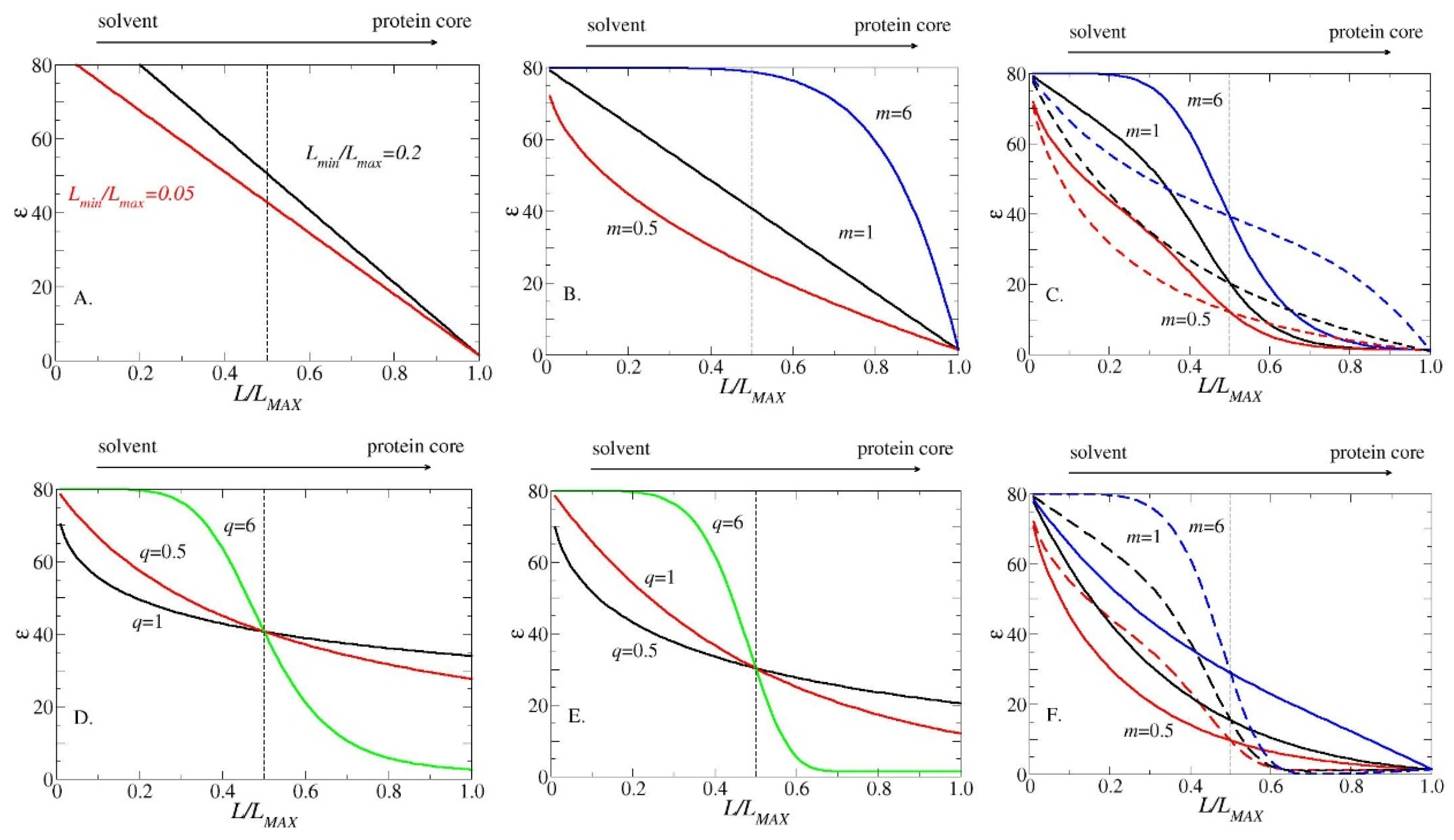
Figure 2.
k-Cindex correlation. The effective permittivity is reported vs. the compactness index, . Calculations were performed on the whole protein sample-set, using different values of the functions’ parameters and interaction radius, . Each panel reports the plot of a different model, A to F, as described in Eqs. (1a-1f). In all panels, colored full symbols refer to data calculated with different values of , from 5 to 12 . In panels C, D,E, F , data obtained using =1 are represented by full symbols and data obtained using =6 are represented by blue empty symbols. In panel B. a continuous yellow line represents the fitting function: (see also Appendix B).
Figure 2.
k-Cindex correlation. The effective permittivity is reported vs. the compactness index, . Calculations were performed on the whole protein sample-set, using different values of the functions’ parameters and interaction radius, . Each panel reports the plot of a different model, A to F, as described in Eqs. (1a-1f). In all panels, colored full symbols refer to data calculated with different values of , from 5 to 12 . In panels C, D,E, F , data obtained using =1 are represented by full symbols and data obtained using =6 are represented by blue empty symbols. In panel B. a continuous yellow line represents the fitting function: (see also Appendix B).
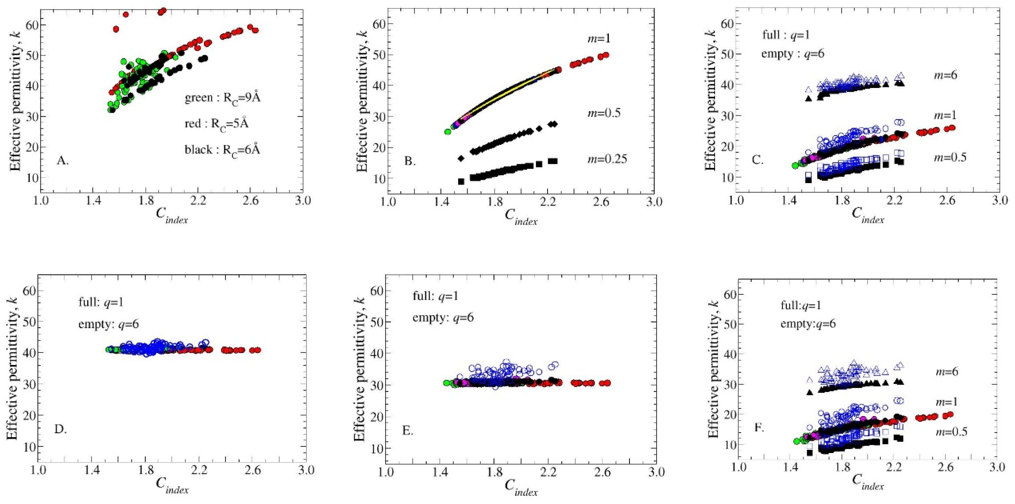
Figure 3.
Effective permittivity calculated for the sample test. The effective permittivity is plotted for the selected proteins and different values of the parameters. A. normalized permittivity evaluated using the six models (A-F); b. Model B is reported using different values of the parameter : both average and variance, calculated on the whole data set are reported; c. Models A,D,E are reported for different values of the parameter; d. Models C,F are reported for different values of the parameters m,q . Notice that data due to are grouped in the bottom set, while data corresponding to are grouped in the upper set. All data were calculated using
Figure 3.
Effective permittivity calculated for the sample test. The effective permittivity is plotted for the selected proteins and different values of the parameters. A. normalized permittivity evaluated using the six models (A-F); b. Model B is reported using different values of the parameter : both average and variance, calculated on the whole data set are reported; c. Models A,D,E are reported for different values of the parameter; d. Models C,F are reported for different values of the parameters m,q . Notice that data due to are grouped in the bottom set, while data corresponding to are grouped in the upper set. All data were calculated using
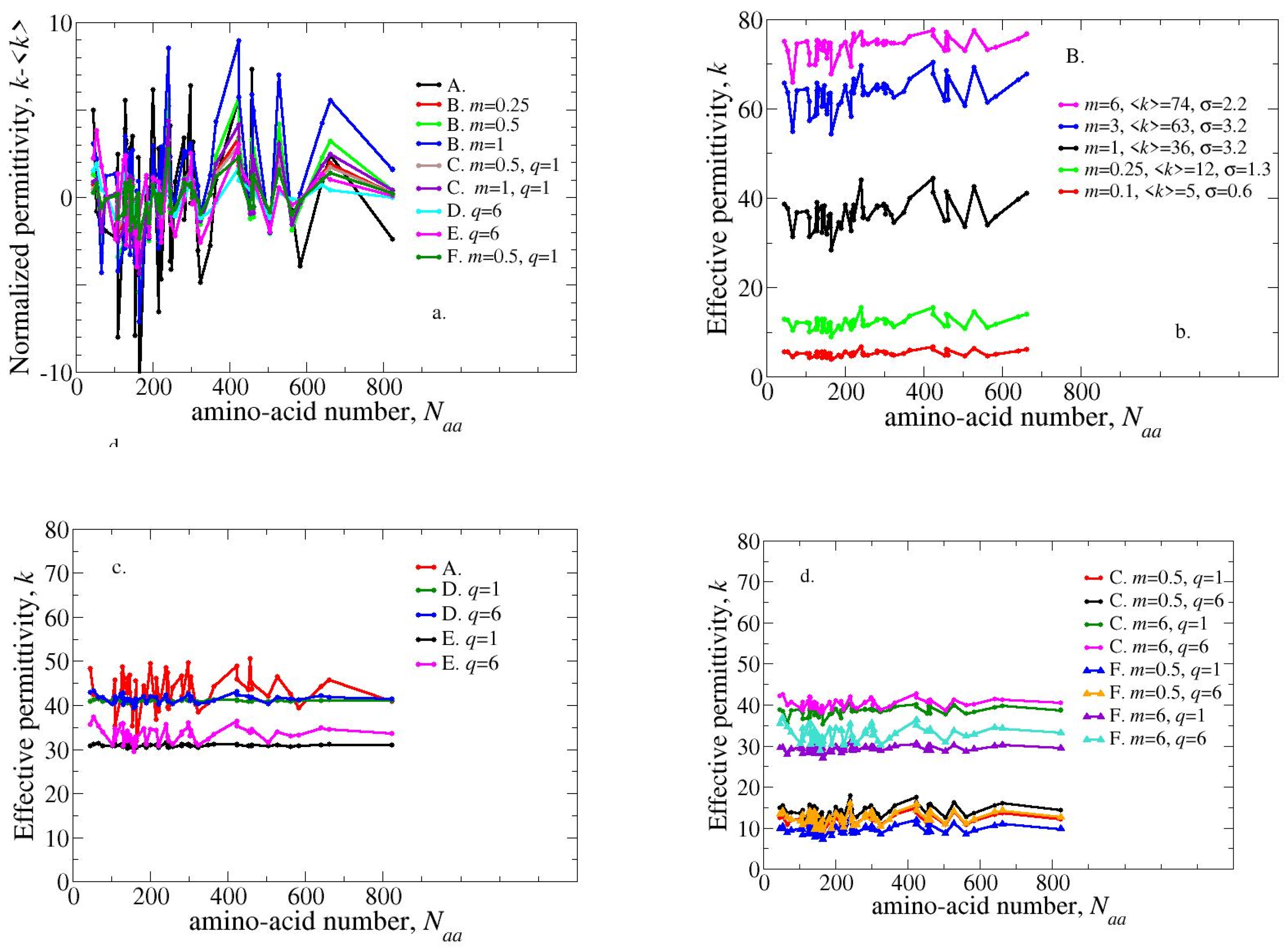
Figure 4.
The normalized imaginary impedance of proteins 1E65, 2L25. Comparison between two different kinds of electrical contacting: up-down (UD: black) and left-right (LR:red). Data were calculated using model B with = 0.25. Imaginary impedance was normalized using the zero-frequency impedance for both proteins. A. apoprotein azurin (PDB code 1E65): the LR contacting produces a slightly smaller value of with respect UD contacting; b. protein NP_888769.1 (PDB code 2L25), the UD contacting produces a value of quite larger than in the LR contacting; c. Impedance is calculated using a single permittivity value for all the amino-acids, i.e., 13 (see Table A1). In the range of frequency 10-100 rad/s the sampling is reduced to better appreciate the differences among the 4 set of data.
Figure 4.
The normalized imaginary impedance of proteins 1E65, 2L25. Comparison between two different kinds of electrical contacting: up-down (UD: black) and left-right (LR:red). Data were calculated using model B with = 0.25. Imaginary impedance was normalized using the zero-frequency impedance for both proteins. A. apoprotein azurin (PDB code 1E65): the LR contacting produces a slightly smaller value of with respect UD contacting; b. protein NP_888769.1 (PDB code 2L25), the UD contacting produces a value of quite larger than in the LR contacting; c. Impedance is calculated using a single permittivity value for all the amino-acids, i.e., 13 (see Table A1). In the range of frequency 10-100 rad/s the sampling is reduced to better appreciate the differences among the 4 set of data.
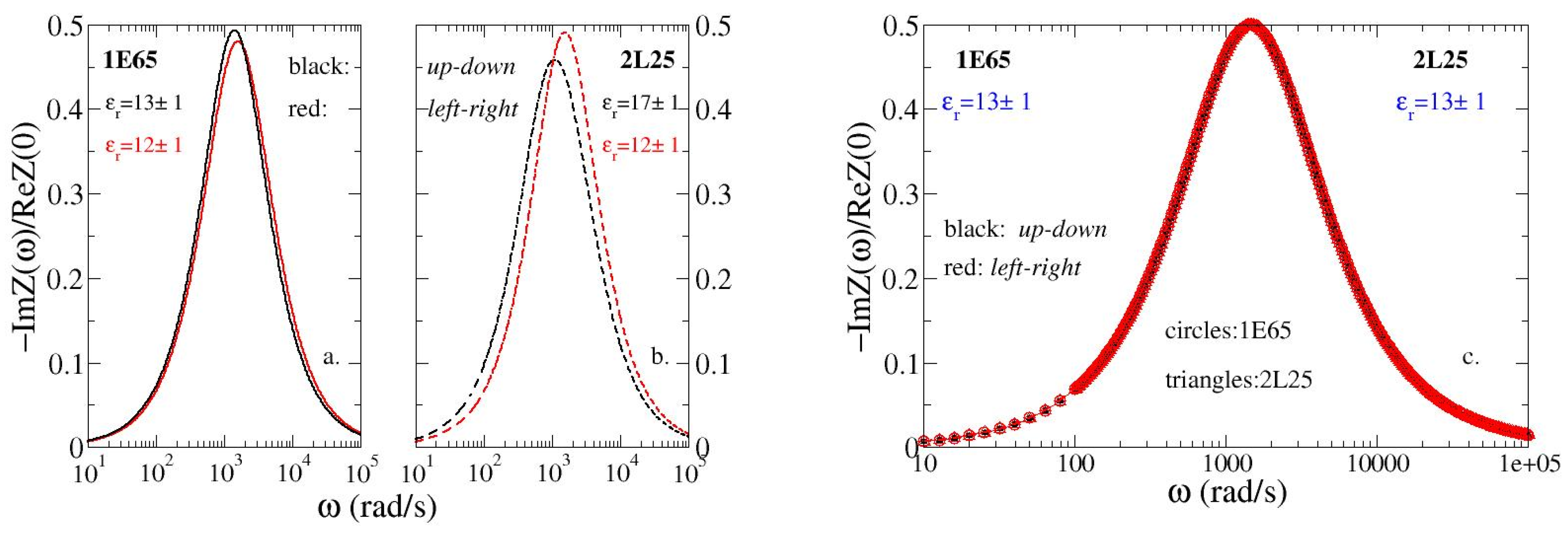
Figure 5.
Graphical representation of proteins 1E65 and 2L25 in two different contact configurations. In both a. and b. panel the left figure represents the protein in the up-down configuration and the right figure represents the protein in the left-right configuration.
Figure 5.
Graphical representation of proteins 1E65 and 2L25 in two different contact configurations. In both a. and b. panel the left figure represents the protein in the up-down configuration and the right figure represents the protein in the left-right configuration.
Disclaimer/Publisher’s Note: The statements, opinions and data contained in all publications are solely those of the individual author(s) and contributor(s) and not of MDPI and/or the editor(s). MDPI and/or the editor(s) disclaim responsibility for any injury to people or property resulting from any ideas, methods, instructions or products referred to in the content. |
© 2026 by the authors. Licensee MDPI, Basel, Switzerland. This article is an open access article distributed under the terms and conditions of the Creative Commons Attribution (CC BY) license (http://creativecommons.org/licenses/by/4.0/).
Copyright: This open access article is published under a Creative Commons CC BY 4.0 license, which permit the free download, distribution, and reuse, provided that the author and preprint are cited in any reuse.