

Submitted:
13 August 2026
Posted:
14 August 2026
You are already at the latest version
Abstract
Grid-based density clustering methods—FlowGrid, FLOPTICS, and grid-accelerated DBSCAN and OPTICS—partition a d-dimensional feature space into an md array of bins and group the non-empty bins by density reachability. They leave a symmetry unexploited: relabelling and reflecting the feature axes permutes the bins while preserving density. We formalise this as an action of the hyperoctahedral group Bd = C2 \( \wr \) Sd of order 2dd! on bin-occupancy functions. We prove that the action preserves the Chebyshev bin-adjacency underlying grid reachability (Theorem 1); that grid density clustering is Bd-equivariant (Theorem 2); that configurations up to symmetry are counted by a Burnside average over Bd (Theorem 3), with an explicit parity-split closed form for the octahedral case at every resolution, which we have not found recorded elsewhere (Theorem 4 and Corollary 2); and that a canonical-form algorithm computes a unique representative per orbit in O (2dd! md) time (Theorem 5). We are explicit about scope: a generic dataset has a trivial stabiliser, so there is no per-run gain; the benefit is canonical indexing, deduplication of symmetry-closed libraries, and caching when the same measurement recurs under a different axis convention. The group specialises to the D4 and Oh symmetries of the DR Code. Symmetry enters twice: as the group acting on the grid, and as the line between symmetric instances and the generic asymmetric ones. All theorems and enumeration formulae are confirmed computationally.
Keywords:
hyperoctahedral group
; grid-based clustering
; density-based clustering
; group action
; equivariance
; Burnside’s lemma
; canonical form
; orbit enumeration
; symmetry reduction
1. Introduction
Clustering is the unsupervised partition of a dataset into groups of similar points; density-based clustering defines those groups as connected regions of high density separated by sparse ones. DBSCAN [1] and its ordering-based refinement OPTICS [2] are the canonical representatives, widely used because they find clusters of arbitrary shape without fixing their number in advance. Their principal cost is the neighbourhood query, and a standard remedy is to impose a regular grid on the feature space, aggregate points into axis-aligned bins, and run the density logic on bins rather than on individual points. FlowGrid [3] and FLOPTICS [4,5,6] are recent members of this grid-based density family; FLOPTICS, in particular, was introduced for the automated gating of flow-cytometry data—a setting in which panels typically measure on the order of ten to forty channels, though gating is usually performed on low-dimensional projections of two to four channels at a time, precisely the regime where is small. Axis relabelling is not a hypothetical symmetry here: the order in which channels are written to a data file, and the orientation conventions of a given instrument or compensation step, are recording choices rather than biological facts, so two laboratories analysing the same sample may present grids differing exactly by an element of . FLOPTICS clusters bins produced by an equal-width partition of each measured channel, and belongs to a family of automated gating methods that includes FLOCK [7], flowPeaks [8], and FlowSOM [9].
A grid is a highly symmetric object. Permuting the feature axes and independently reflecting any axis sends bins to bins and leaves every notion of grid adjacency intact. The collection of these operations is a finite group—the hyperoctahedral group of order , classically the symmetry group of the -cube and of the integer lattice , and the natural symmetry acting on functions over a product space of the kind studied in [10]; the underlying integer-lattice geometry is standard [11]. Although grid-based clustering algorithms operate directly on this symmetric object, they treat the axes as ordered and oriented, so the symmetry is present in the problem but absent from its analysis. The purpose of this paper is to make the symmetry explicit and to derive its exact consequences for the enumeration, canonicalisation, and reproducibility of grid-clustering instances.
Our motivation is concrete and recent. In a companion study of the DR Code—a two-dimensional barcode whose block layout admits XOR-based strip recovery [12]—the authors showed [13] that the recoverable layouts form the orbit space of an order-72 group and that passing to orbit representatives compresses the layout catalogue and yields a canonical-form deduplication scheme. The geometric part of that group is exactly , the symmetry group of the square. A companion study extends the code to a logical cube, where the corresponding symmetry group is of order and the geometric factor is the full octahedral group of the cube [14]. Both are instances of the hyperoctahedral family: and . The present paper takes the natural next step by removing the barcode-specific recoverability constraint and studying the pure grid symmetry in the setting where the grid hosts a clustering instance rather than a constrained code. In doing so we move from a finite constrained catalogue to the unconstrained—and unbounded—space of bin-occupancy functions, which changes both the enumeration problem and the meaning of a canonical form.
We are careful about what symmetry buys. A generic occupancy function has trivial stabiliser, so its orbit has full size and no bins are forced to coincide; we therefore make no per-run speedup claim. The orbit structure is instead useful across instances—canonical indexing, deduplication of symmetry-closed libraries, and caching across analyses that present the same measurement under a different axis convention—and we quantify these benefits.
A second motivation is reproducibility. Grid-based clustering pipelines are increasingly deployed as standardised tools—FLOPTICS, for instance, is intended as a reproducible alternative to subjective manual gating—and reproducibility requires that the output not depend on incidental choices such as the order in which feature channels happen to be listed or the sign convention of an axis. Equivariance under is the exact statement that these choices are incidental: two operators who list the channels in different orders, or orient an axis oppositely, obtain clusterings differing by precisely the corresponding relabelling. A canonical axis order removes this degree of freedom and makes the pipeline deterministic with respect to axis presentation. This is a modest but genuine guarantee, and it falls out of the same group action that governs the enumeration and caching results.
Two questions organise what follows. (Q1) In what precise sense is grid-based density clustering independent of how the feature axes happen to be ordered and oriented, and what is the group that expresses this? (Q2) Given that group, how many genuinely distinct clustering instances are there on a grid, and can each be given a canonical name cheaply enough to be useful? Q1 is answered by the equivariance theorem, Q2 by the enumeration and canonical-form results.
The contributions of this paper are the following. (C1) We formalise the action of on bin-occupancy functions and prove that it preserves the Chebyshev bin-adjacency that underlies grid density reachability (Section 4, Theorem 1). (C2) We prove that grid-based density clustering is -equivariant: relabelling the axes relabels the clusters and nothing more (Section 5, Theorem 2). (C3) We give a Burnside/cycle-index count of bin-occupancy configurations up to , specialise the classical signed-cycle-type computation of the cycle index of to the grid ; the resulting closed form for the octahedral case, valid at every resolution and split by the parity of the resolution, is our main enumerative contribution and we have not found it recorded elsewhere. The dihedral case () is derived the same way as a worked illustration, and we verify all of it against exhaustive orbit enumeration (Section 6, Theorems 3 and 4, Corollary 2). (C4) We present a canonical-form algorithm (Algorithm 1), prove its correctness and complexity, and delimit its honest range of usefulness (Section 7, Theorem 5). Throughout, two supporting propositions record the orbit-size structure (Proposition 1) and the asymptotic orbit count (Proposition 2), and a fully worked micro-example makes every ingredient checkable by hand. Section 2 reviews related work, Section 3 fixes notation, Section 8 discusses scope and applications, and Section 9 concludes. In total we prove five theorems, one lemma, two propositions and four corollaries, and give two algorithms. Every quantitative claim in the paper was checked computationally using the open-source scripts released with the paper—exhaustively on the relevant finite structures wherever they are small enough to enumerate, and by large randomised trials elsewhere.
2. Background and Related Work
2.1. Density-Based and Grid-Based Clustering
DBSCAN defines clusters through core points, whose -neighbourhood contains at least a threshold number of points, and the density-reachability relation they induce. OPTICS replaces the single global by an ordering of the points annotated with reachability distances, from which clusterings at multiple density levels can be extracted [2,15]. Both incur neighbourhood queries whose naïve cost is quadratic and whose spatially indexed cost is [16]. Grid-based methods sidestep the query by bucketing points into a regular array of bins: FlowGrid and FLOPTICS partition each dimension into equal-width intervals, keep only non-empty bins, and apply density logic to bin counts and bin adjacency; this generalised density-based view, in which clusters are connected dense cells of a space partition, goes back to GDBSCAN [17]. FLOPTICS specifically runs an OPTICS ordering over the occupied bins, so the clusters it extracts are determined by bin counts and the Chebyshev adjacency of the grid—the two ingredients our model retains—while discarding sub-bin coordinates [4,5,6]. This reduces the working set from points to the number of occupied bins and replaces metric neighbourhood tests by index arithmetic. The methods we analyse are exactly of this grid-based density type [3,4,5,18]; our results apply to any algorithm whose clusters are determined by bin occupancy and grid adjacency.
Table 1 lists the methods in this family and what our model retains from each.
To make the object of study concrete, Figure 1 illustrates the grid-based density-clustering pipeline on a three-cluster synthetic example in the style of automated flow-cytometry gating. A reachability ordering (panel a) exposes the cluster structure as valleys; the feature space is discretised into an axis-aligned grid whose non-empty bins are the working set (panel b); and the clusters recovered on that grid correspond to the dense regions of the original data (panel c). The figure is schematic and carries no experimental claim—the empirical evaluation of FLOPTICS itself is reported in its source work [4,5,6]—but it fixes the picture our analysis depends on: everything downstream is determined by which bins are occupied and how they are adjacent, and it is precisely this grid, panel (b), on which the hyperoctahedral group acts in the remainder of the paper.
2.2. Symmetry of the Grid and the Hyperoctahedral Group
The symmetry group of the hypercubic lattice —equivalently of the -cube—is the hyperoctahedral group of all signed permutation matrices, , of order . Its elements are the signed permutations: a permutation of the axes composed with an independent choice of reflection on each axis. In the combinatorial literature is the group of the “signed” or “hyperoctahedral” symmetric functions, and its cycle index is the classical tool for enumerating structures on the cube and lattice [19,20,21]. We use in precisely this role, but applied to the array of clustering bins rather than to the cube’s vertices.
2.3. Orbit Enumeration by Burnside’s Lemma
Counting configurations up to a group action is governed by the Cauchy–Frobenius–Burnside lemma: the number of orbits equals the average number of configurations fixed by a group element [22,23]. When configurations are colourings of a set acted on by a group, the count is delivered by Pólya’s cycle-index theorem [24,25]; general treatments appear in [21,26,27]. These techniques have been applied to lattice-square designs [28], whose isomorphism group is built from a hyperoctahedral and a dihedral factor and whose classes are counted by Burnside; to the enumeration of polyomino symmetry classes on the square lattice under and [29]; and to the classification of full-dimensional -polytopes through the cycle index of [30]. Our enumeration (Theorem 3) is a Burnside average over acting on occupancy functions; it is methodologically classical, and our contribution is its transfer to, and interpretation for, clustering instances rather than any new counting machinery.
2.4. Canonical Forms and Reproducibility
A canonical form assigns to each object a unique representative of its equivalence class, so that two objects are equivalent exactly when their canonical forms coincide. Canonical labelling of graphs (the individualisation–refinement algorithms behind nauty and Traces) [31] and canonical string encodings of molecules (canonical SMILES) [32] are the standard instances; both underpin database deduplication, indexing, and reproducible pipelines. Our canonical form (Theorem 5) is of the same spirit but for a far smaller and fully explicit group: because is fixed and independent of the data, canonicalisation is a bounded loop over group elements rather than a search over an exponential automorphism space, and its correctness is immediate. This is the practical contrast with general graph canonicalisation: the individualisation–refinement search behind nauty and Traces may, in adversarial cases, backtrack through exponentially many candidate labellings, whereas the canonical form used here performs exactly push-forwards with no backtracking and no data-dependent branching, so its cost is a fixed constant (, , for ) times the grid size.
2.5. Relation to the DR Code
The recoverable layouts of the DR Code form the orbit space of a group of order 72, whose geometric factor acts by rotating and reflecting the square grid while the cyclic factor permutes row and column labels subject to the recoverability constraint [13]. The present paper isolates the geometric factor and generalises it: we drop the recoverability constraint, replace the fixed board by an arbitrary grid, and replace by the full hyperoctahedral group . Two differences are worth stating plainly. First, the DR Code group mixes a geometric () and a combinatorial () factor tied to its recoverability rule; our group is purely the geometric grid symmetry , appropriate because a clustering grid carries no analogue of the row/column-label constraint. Second, the DR Code acts on a finite constrained set of 2,592 layouts, whereas acts on the unbounded space of occupancy functions, so our enumeration is parameterised by grid resolution and occupancy alphabet rather than being a single finite number. The DR Code is thus the , constrained special case that motivates the unconstrained, general- theory developed here.
Table 2 situates the present work among prior applications of hyperoctahedral and lattice symmetry. The machinery—signed permutations with Burnside/cycle-index counting—is shared; what is new is the object and its purpose: an unbounded space of clustering instances analysed for canonical indexing and equivariant reproducibility rather than a finite classification.
2.6. Relation to Equivariant Machine Learning
The idea that a model should respect the symmetries of its input is central in modern machine learning: group-equivariant convolutional networks [35] build layers that commute with a symmetry group, and the geometric-deep-learning programme [36] organises architectures around this principle, with grids as the prototypical example. Theorem 2 is a statement of the same kind for a classical clustering procedure rather than a learned network, with two differences: our grids are finite and unpadded, so the relevant group is the finite point group rather than a translation group; and the payoff here is enumerative rather than sample efficiency. A third connection is data augmentation—a -closed library is exactly an axis-augmented suite, so the deduplication of Section 8 says such a suite carries no more information than its canonical reduction. Hierarchical methods such as HDBSCAN [15] share the same structure on a binned space, so the results apply to them unchanged.
3. Preliminaries
For convenience, Table 3 collects the notation used throughout.
Fix a dimension and a per-axis resolution . The grid is the set of bins
Two bins are adjacent, written , if they differ and are within Chebyshev distance one, i.e. and . This is the king-move adjacency used by grid-based density clustering to decide when two occupied bins belong to the same dense region.
An occupancy function is a map into a finite alphabet of size ; records the point count of bin , optionally quantised into density levels, with denoting an empty bin. The set of occupancy functions is , of size .
It is convenient to record two special cases immediately. At the group has order and is the dihedral group of the square: the two axis reflections and the axis swap generate the four rotations and four reflections of a square grid. At the group has order and is the full octahedral group of the cube. These are exactly the geometric symmetry groups appearing in the 2D and 3D DR Code, which is the sense in which the hyperoctahedral action generalises that setting to arbitrary dimension.
We also fix the cycle-index notation used in Section 6. For a permutation of a finite set write its cycle type as the formal monomial , where is the number of -cycles of . The cycle index of a group acting on is . Setting every evaluates the cycle index to with the total number of cycles; by Theorem 3 this is the number of -colourings of up to .
The hyperoctahedral group is
realised as signed permutations. We write an element as a pair with a permutation of axes and a per-axis reflection sign. Composition follows the wreath-product rule: for and one has with , and the identity is . We use two standard facts about a finite group acting on a set: the orbit of a point is , its stabiliser is , and the orbit–stabiliser theorem gives ; and the number of orbits is the Burnside average of fixed-point counts. Both are applied below to acting on occupancy functions.
4. The Group Action on Grid Bins
We first make act on bins, then on occupancy functions, and verify the action respects grid adjacency—the property that makes it compatible with density reachability. The three generating operations are shown schematically in Figure 2.
Definition 1 (action on bins). For and a bin , define by
Thus permutes the axes by and reflects the selected axes. The induced action on occupancy functions is by push-forward, .
Theorem 1 (well-defined adjacency-preserving action). The map of Definition 1 is a left action of on by bijections, and it preserves adjacency: for every . Consequently the push-forward is a left action of on , and it preserves the bin-adjacency graph on which grid density reachability is defined.
Proof. Each single-axis reflection is an involution of , and axis permutation by is a bijection of coordinate positions; their combination is therefore a bijection of , with inverse where . The identity acts as the identity map, and a direct computation shows , so the map is a left action. For adjacency, write . Axis permutation only relabels the coordinates, so it permutes the multiset and leaves its maximum unchanged. A reflection on axis replaces by , whose absolute difference is again . Hence is invariant and , so . The push-forward inherits the action axioms from the action on bins, and because adjacency is preserved, the bin-adjacency graph is mapped isomorphically to itself.
We verified Theorem 1 exhaustively: for and several resolutions , all elements act as bijections of , the wreath-product composition rule agrees with the composition of the corresponding bin-maps on every bin, and every adjacent pair maps to an adjacent pair. At the group has order and coincides with ; at it has order and coincides with —precisely the geometric groups of the 2D and 3D DR Code (Table 4).
To make the action concrete, take and , and index the nine bins in row-major order so that bin receives index . The axis swap with trivial signs sends ; as a permutation of bins it is the transposition pattern fixing the diagonal and swapping , , , i.e. a matrix transpose. The reflection of axis with trivial permutation sends , exchanging the top and bottom rows. Composing the eight signed permutations of reproduces precisely the eight symmetries of the square acting on the board, confirming at the level of the bin permutation representation. The same construction at , enumerates the bin permutations of on the -cell cube.
5. Equivariance of Grid Density Clustering
We now show that clustering commutes with the group action, after fixing the model precisely.
Definition 2 (grid density clustering).Fix a density threshold. A binis dense for the occupancy functionif; writefor the set of dense bins. The grid density clustering ofis
a partition of into clusters, where is the Chebyshev adjacency ofSection 3. This is the grid-based, single-threshold specialisation of density clustering that FlowGrid applies directly and that an OPTICS-based method such as FLOPTICS yields when clusters are extracted at a fixed reachability level; it is determined by the pair (which bins are dense, which dense bins are adjacent) and by nothing else. The intermediate reachability ordering produced by OPTICS is not itself claimed to be canonical: it may depend on processing order and tie-breaking, whereas the extracted clustering treated here does not.
With Definition 2 in place, the equivariance statement is immediate to formulate.
Theorem 2 (equivariance).For everyand every occupancy function,
whereacts on a partition by acting on each of its bins. In particular the number of clusters and the multiset of cluster sizes are-invariant, and the cluster containing binis mapped byto the cluster containing.
Proof. A bin is dense for iff , i.e. iff is dense for ; thus the dense set of is the -image of the dense set of . By Theorem 1 the map is an adjacency graph isomorphism, and a graph isomorphism carries connected components to connected components bijectively. Therefore the components of the dense set of are exactly the -images of the components of the dense set of , which is the claimed identity . The stated invariants follow because a bijection preserves cardinalities.
Corollary 1 (invariance of clustering summaries).Every function of a clustering that depends only on the multiset of cluster sizes—the number of clusters, the largest cluster size, the number of clusters exceeding a given size, and any index or entropy computed from the size distribution—is a -invariant of the occupancy function, hence constant on orbits and tabulable per orbit rather than per instance.
Proof. By Theorem 2 the clustering of is the image of the clustering of under the bijection . A bijection preserves the multiset of block sizes, so any function of that multiset agrees on and for every , i.e. is constant on the orbit.
Equivariance is the precise sense in which the ordering and orientation of the feature axes are irrelevant to the clustering: relabelling the axes relabels the output and changes nothing else. This has an immediate practical reading. A pipeline that fixes a canonical axis order (Section 7) produces identical clusters regardless of the order in which channels were originally recorded, removing a spurious source of run-to-run variation. We verified Theorem 2 on (occupancy, group-element, threshold) triples— with and with , using randomised thresholds: in every case the partition of equalled the -image of the partition of . Figure 3 depicts the commuting square that the theorem asserts.
6. Enumeration of Bin-Occupancy Classes
Because clustering is -equivariant, two occupancy functions in the same orbit are indistinguishable up to axis relabelling and yield the same clustering up to that relabelling. It is therefore natural to count occupancy functions up to . Let denote the number of orbits of on with .
Theorem 3 (Burnside enumeration).The number of bin-occupancy configurations on thegrid up tois
whereis the number of cycles ofacting as a permutation of thebins. Equivalently,, the cycle index of the bin-permutation representation ofevaluated with every variable set to.
Proof. The group acts on the finite set of colourings of by colours through the push-forward. By the Cauchy–Frobenius–Burnside lemma the number of orbits equals the average number of fixed colourings, . A colouring is fixed by iff it is constant on each cycle of ’s action on ; the number of such colourings is , one free colour choice per cycle. Summing gives the stated formula, and rewriting the cycle-count distribution as a cycle-index polynomial yields the evaluated cycle index.
The building blocks of are elementary and let the practitioner evaluate the sum without enumerating all bins. On a single axis of length , a non-reflected axis contributes the identity permutation ( fixed points) while a reflected axis contributes transpositions and fixed points; the cell-cycle structure of a signed axis permutation is the product of these one-dimensional structures composed with the axis permutation , exactly as in the wreath-product cycle index of . We confirmed the one-dimensional reflection count for and, more importantly, verified that the Burnside formula agrees with brute-force orbit counting in every small case: for instance , , , and , each matching a direct orbit enumeration. Table 5 lists representative values, and Figure 4 contrasts the orbit count with the raw count , showing the expected reduction by a factor approaching as the configurations become generic.
The cycle index via signed cycle types. The Burnside sum of Theorem 3 is governed by the cycle count , and depends only on the signed cycle type of : the multiset of pairs , one per cycle of the axis permutation , where is the cycle length and is the product of the reflection signs around that cycle. That the induced cycle structure of a signed permutation is determined by this data is classical: the cycle index of was first obtained by Harrison and High [33] and given in a simpler form by Chen [34], who computes the induced cycle structure on the vertex set of the hypercube from the signed cycle decomposition. What we need here is the same computation for the grid with arbitrary resolution ; the case recovers the classical hypercube-vertex setting. We record the specialisation for completeness, since the -dependence is what drives the enumeration below.
Lemma 1 (the block map and its cycle-length multiset). Let a cycle of have length and net sign . On the corresponding factor it induces the map
Thenis a permutation ofof orderwhenandwhen; writefor its multiset of cycle lengths. Every cycle length divides the order of, and the multiplicities are recovered from the fixed-point counts by Möbius inversion,
For these counts are , so the total number of cycles is . For the wrap-edge reflection makes the counts depend on the parity of , and is obtained from the same inversion. Explicitly, fixes a point exactly when the point is constant along the orbits of the -fold shift and, when is odd, additionally reflection-symmetric in each such orbit, so when is even, and otherwise; the cycle multiplicities of then follow by the same Möbius inversion. For this gives the familiar pair and .
Proof of Lemma 1. is a composition of a slot rotation with (for ) an involution of one coordinate, hence a permutation of the finite set . For , is the identity and no smaller power is, so ; a point is fixed by exactly when it is constant along the orbits of the shift by , of which there are , giving , and the total cycle count is the classical necklace count . For , applies the reflection to every coordinate—an involution with fixed points—and , so and the fixed-point counts, hence the cycle lengths, depend on the parity of . In both cases the cycle lengths divide and the stated Möbius inversion is the standard recovery of exact-period counts from fixed-point counts.
Theorem 4 (cycle index ofon the grid ). Forwith signed cycle type , letbe the cycle-length multiset of the block map of Lemma 1. Then the number of cycles ofon the full gridis
the product-action count taken over one cycle chosen from each block. Consequentlyis, for fixed, a quasi-polynomial inof degreein the exponent with period dividing.
Proof. Distinct -cycles act on disjoint coordinate blocks, so is the direct product of the block maps and the grid factorises as . For a direct product of permutations, one cycle chosen from each factor with lengths generates on their joint support exactly cycles—the orbit count of the diagonal generator of —and summing over all tuples gives . The block count is the necklace formula stated in Lemma 1; the block introduces a reflection on the wrap edge whose effect depends on the parity of , so the exponents are quasi-polynomials of period , with leading term from the identity.
The formula is the evaluation at of the cycle-index polynomial of the bin permutation representation. Read representation-theoretically, counts the -fixed colourings, so is the dimension of the space of -invariant functions on —the invariant-theoretic quantity whose graded analogue is computed by a Molien series. We do not pursue the graded version, but it is the natural route to refinements such as counting occupancy classes by the number of occupied bins.
The formula specialises the classical hypercube computation of [33,34] to arbitrary , and we verified it exhaustively: for all and all and every resolution , the product-action formula reproduces the directly counted in all cases.
Worked cycle index at . We derive in closed form to illustrate the cycle-index computation. The group has eight elements acting on the bins: the identity ; the two axis reflections ; their product (the rotation); the axis swap (matrix transpose); and the three remaining signed swaps , , (the rotations and the anti-diagonal reflection). Counting cycles on the board:
- fixes all bins, contributing .
- Each axis reflection acts independently on each of the lines parallel to it, splitting the bins of every such line into transpositions together with fixed bins, i.e. cycles per line, giving ; the two such elements contribute .
- The rotation fixes the centre bin when is odd and pairs the rest, giving , contributing .
- The transpose fixes the diagonal bins and pairs the off-diagonal transposed pairs, giving ; likewise the anti-diagonal reflection. These two contribute .
- The two rotations have -cycles off the centre and one fixed centre when is odd, giving ; they contribute .
Hence
For , this evaluates to , matching the exhaustive orbit count. For , it gives , and for , it gives ; both agree with direct enumeration (Table 5). At q = 2 the formula counts binary square arrays up to the symmetries of the square; the resulting sequence is recorded as A054247 in the OEIS [37], and our expression reproduces every term listed there. We have not found a tabulation for general alphabet size, but we claim no novelty for the two-dimensional case: it is included as a worked illustration of the cycle-index computation.
A fully worked micro-example ( , ). The smallest non-trivial case can be checked entirely by hand and illustrates every ingredient. Here has bins, has elements, and with binary occupancy there are raw patterns. Burnside gives , and the six orbits are listed in Table 6 together with their sizes and stabiliser orders. The orbit sizes sum to , and each satisfies the orbit–stabiliser relation : for example the two-bins-on-a-diagonal pattern has stabiliser of order (the diagonal is fixed setwise by the identity, the two reflections across the diagonals, and the rotation) and hence an orbit of size .
The relation visible in the table is a special case of the orbit-counting decomposition, and provides an independent arithmetic check on any Burnside computation.
Two further structural facts are worth recording. First, for fixed the count is a polynomial in of degree whose coefficients are non-negative rationals summing appropriately; for instance and , which is the generating function of occupancy classes graded by alphabet size. Second, the orbit sizes are not uniform: at , , the six orbits split as two of size , one of size , and three of size , whereas by the orbit-size distribution is orbits of size , of size , of size and of size , so of the orbits still have non-trivial stabiliser—a proportion that, by Proposition 2, tends to zero as or grows. The small grids are thus the exception in which symmetry is abundant; the generic large-grid instance sits in a full-size orbit.
Figure 5 shows these distributions directly.
Proposition 1 (orbit sizes divide the group order). For every occupancy function , the orbit has size , a divisor of ; in particular every orbit size divides , and the generic orbit (trivial stabiliser) has the full size .
Proof. This is the orbit–stabiliser theorem applied to acting on : the map is a bijection from left cosets of onto the orbit, so , which divides by Lagrange’s theorem. When is trivial the orbit attains the full size.
Corollary 2 (closed form at , the octahedral case).Applying Theorem 4 to —whoseelements fall into ten conjugacy classes (identity, face and edge reflections,andface rotations,vertex rotations, the central inversion, and their compositions)—yields an explicit closed form for every resolution, split by the parity of . Foreven,
and for odd,
Setting gives and ; setting gives . All three, and the values up to , (a -digit integer), were confirmed against independent orbit enumeration. Two remarks place this formula. First, at the grid is the vertex set of the cube and the count reduces to the classical enumeration of -colourings of the cube vertices under , giving ; that case is standard. Second, for —the regime that matters for clustering grids—we are not aware of a published closed form, and the parity split above appears not to have been recorded, though the ingredients are entirely classical. Unlike its two-dimensional counterpart, the sequence of values it produces returns no match in the OEIS [37] (searched 28 July 2026), whereas the two-dimensional sequence is recorded there as A054247. We therefore present it as an explicit specialisation rather than a new enumerative technique. In general, as the resolution or the alphabet grows, the identity term dominates the Burnside sum and
so the number of distinct configurations approaches the raw count divided by the full group order . We state this precisely.
Proposition 2 (asymptotic orbit count). For fixed , as (or as with ), .
Proof. The identity element contributes to the Burnside sum, while every non-identity has (it moves at least one bin, merging at least two of them into a common cycle). More sharply, every non-identity element satisfies with the largest non-identity cycle count identified below, so the total non-identity contribution is at most , which is an fraction of the identity term whenever . Both limiting regimes now follow. For fixed , the ratio is and vanishes as . For fixed , the gap is itself unbounded in : the largest non-identity cycle count is attained by a single axis transposition, which fixes the bins whose two transposed coordinates agree and pairs up the rest, giving and hence a gap of , which tends to infinity with for every fixed . Consequently tends to zero as well. Dividing by gives the claim. ■
Remark 1 (the second-order term). The correction can be made completely explicit. Write for the largest cycle count attained by a non-identity element and for the number of elements attaining it. Then the two-term expansion reads
and the relative error is therefore
At we have , so the decay exponent is ; the value is attained by the two diagonal reflections for every , joined by the two axis reflections when is odd, giving for even and for odd. At we have and decay exponent ; here the value is attained by the six diagonal mirror planes—the three pure axis transpositions together with the three that also flip the two swapped signs—for every , joined by the three face reflections when is odd, giving for even and for odd. Numerically, at , , the neglected terms contribute a relative against the predicted , and at , , a predicted .
This asymptotic is the precise statement that “almost all” occupancy functions have trivial stabiliser and therefore full-size orbits—the same fact that, read from the algorithmic side, tells us there is no per-instance bin collapse to exploit on generic data (Section 7). Figure 4 shows the finite- approach to this ratio.
The case , , is a useful anchor: there are distinct empty/non-empty bin patterns on a grid up to . This is the clustering-grid counterpart of the DR Code’s orbit counts on the same board, with the recoverability constraint removed and the alphabet reduced to “empty vs. occupied”.
7. Canonical Form and Complexity
Enumeration counts orbits; applications need a way to name them. We give a canonical form—a function constant on orbits and injective across them—together with its cost.
Definition 3 (canonical form). Order lexicographically by reading bin values in a fixed bin order. For an occupancy function define
the lexicographically smallest function in the orbit of , and let be a group element attaining the minimum.
Algorithm 1 makes the computation in Definition 3 explicit. It enumerates the signed permutations, applies each to the occupancy function, and keeps the lexicographically smallest image together with the group element that produced it.
| Algorithm 1: Canonical form of an occupancy function under |
| Input: occupancy function on the grid |
| Output: canonical form and a witness with |
| 1. ; |
| 2. for each signed permutation do |
| 3. compute the push-forward (relabel all bins) |
| 4. if or then ; |
| 5. return |
The loop runs exactly times; each iteration relabels bins and performs one lexicographic comparison of length , so the total cost is time and working space, as stated in Theorem 5. Because the group is enumerated in full, the algorithm is deterministic and its worst case coincides with its every case; there is no data-dependent search. Two complementary remarks bound this cost from below and from above in the typical case. For the lower bound, any correct canonical form must inspect essentially the whole grid: at , , , flipping any single one of the nine bins changes the canonical form; the same holds on any grid, since altering one bin changes the multiset of occupancy values, which is an orbit invariant. Consequently no algorithm can decide the canonical representative after reading bins, and the factor in Theorem 5 is unavoidable—only the group factor is specific to our method. For the typical case, the lexicographic comparison in step 4 aborts at the first differing bin, which on random occupancy data happens after bins; measured over random instances the total work falls to a little over half of the naive bound that charges a full-length comparison to every group element (0.51–0.64 across the parameter range we tested), with the push-forwards, not the comparisons, dominating.
Theorem 5 (canonical form: correctness and complexity).The mapsatisfiesfor all, andif and only iflies in the orbit of. It can be computed intime andworking space by evaluating thepush-forwards and retaining the lexicographic minimum. The number of distinct canonical forms over all occupancy functions equalsof Theorem 3.
Proof. For invariance, the orbit of equals the orbit of , so the minimum over the orbit is the same function; hence . For separation, if then and share an orbit element and therefore share an orbit; conversely if they share an orbit they share its unique lexicographic minimum. The algorithm iterates over the group elements; each push-forward relabels bins and the lexicographic comparison is linear in , giving time, while only the current best function and the candidate are stored, giving space. Since is constant on orbits and distinct across them, the number of images equals the number of orbits, which is by Theorem 3.
Two consequences are worth stating separately, since they are what a downstream system actually uses.
Corollary 3 (uniqueness of the normal form).Each-orbit contains exactly one occupancy function that is its own canonical form, namelyfor anyin the orbit; and. Henceis a well-defined normal form: it selects one and only one representative per orbit, and applying it twice changes nothing.
Proof. Existence: for in the orbit, lies in the orbit (it is for some ) and is the lexicographic minimum of that orbit. Idempotence: since lies in the same orbit, is the minimum of the same finite totally ordered set, so . Uniqueness: if in the orbit satisfies then is the minimum of the orbit, and a totally ordered finite set has exactly one minimum, so .
Corollary 4 (orbit membership test).For occupancy functionson the same grid,if and only if . The test therefore coststime in general, and only —a single key comparison—when canonical forms have already been computed and stored, as they are in the indexing and caching applications ofSection 8.
Proof. If then the two orbits coincide and hence so do their lexicographic minima. Conversely, equal canonical forms mean and share an orbit member, and orbits are either equal or disjoint, so the orbits coincide and . The cost is that of two applications of Algorithm 1 plus one comparison of length , which is ; when the canonical forms are cached, only the comparison remains.
We verified Corollary 4 directly: over random pairs at , the canonical-form test agreed with an exhaustive search over all in every case.
Two features distinguish this canonical form from general graph or molecule canonicalisation: the group is fixed and explicit, so the loop length depends only on the ambient dimension and no search over an unknown automorphism group is needed; and the cost is modest in the low dimensions where grid clustering is used—, , . Table 7 lists the group size and resulting cost in the low dimensions relevant to grid clustering. We verified correctness computationally—exhaustively over all binary occupancy functions of the smallest grid, and on random instances for : applying any before canonicalising never changed the result, and functions sharing a canonical form always shared an orbit.
A worked example. Consider , , binary occupancy (empty/occupied). There are raw occupancy patterns and, by the formula above, orbits under . Take the pattern with occupied bins (an L-shaped corner cluster). Its -orbit consists of this corner L pointed into each of the four corners of the board, four distinct patterns in all: the pattern is fixed by the reflection across the main diagonal through its occupied corner, which swaps and fixes , so its stabiliser has order and its orbit has size by the orbit–stabiliser theorem. The canonical representative is the lexicographically smallest of the four; because empty bins carry the smallest alphabet value, the minimum is the image that pushes the occupied bins as late as possible in the bin order, namely the L occupying the opposite corner, and every one of the four input patterns canonicalises to it. A downstream index that keys clustering results by this canonical corner stores and computes the result once rather than four times. A generic (asymmetric) occupancy pattern would instead have trivial stabiliser and a full orbit of size ; the corner L is one of the of the orbits with non-trivial stabiliser recorded in Section 6, which is precisely why its orbit is smaller. This is the mechanism of Theorem 5 in miniature, and it is exactly what a -closed augmentation of a benchmark suite triggers at scale.
The three-dimensional case is equally concrete. On the cube (, ) under , a single occupied corner has orbit size (the eight cube corners) and stabiliser of order —the subgroup permuting the three axes that meet at that corner. Two occupied corners sharing an edge form an orbit of size with stabiliser of order , and a fully occupied face (four corners) has orbit size with stabiliser of order . These are exactly the vertex, edge, and face orbits of the cube, recovered here as occupancy classes; canonicalising any member of each orbit returns the same lexicographically minimal representative.
Scope of the benefit. The canonical form does not accelerate a single clustering run: on a generic occupancy function the stabiliser is trivial, the orbit has full size , and there is nothing to collapse within one instance. We measured the fraction of random occupancy functions with a non-trivial stabiliser and found it falls rapidly toward zero as the grid and alphabet grow: at , , it was already over the sampled instances (Figure 6a). The orbit structure pays off, instead, across collections of instances. In a benchmark library closed under —for example a synthetic suite augmented by axis permutations and reflections, a common way to test rotation/reflection invariance—canonicalising removes the redundant members: a library of instances built as full orbits of seeds collapses to exactly canonical instances, an reduction equal to the average orbit size, drawn as the dashed reference line in Figure 6b. That factor is a construction, not an observation: the library was built from complete orbits, so it verifies that the bound of Definition 4 is attained and nothing more. The complementary question—whether symmetry-equivalent instances arise by chance in a workload that was not built that way—we settled by measurement, and the answer is essentially no. Over 20,000 independently drawn occupancy functions we compared the number of distinct functions with the number of distinct canonical forms, so as to isolate what canonicalisation adds beyond hashing the occupancy function itself. The additional factor was 5.02 at d = 2, m = 3, q = 2 and 2.25 at m = 4, but it fell to 1.002 at m = 5, 1.000 at m = 6, 1.004 at d = 3, m = 3, q = 2, and 1.000 at both d = 2, m = 4, q = 4 and d = 3, m = 3, q = 4 (Figure 6b). The early values are an artefact of a workload larger than the instance space: at d = 2, m = 3, q = 2 the 20,000 draws saturate all 512 patterns, which collapse to the 102 orbits of Table 5. Once the space is large relative to the workload—which is the case at every resolution of practical interest—symmetry-based deduplication adds nothing to ordinary hashing. It pays only on workloads that are deliberately symmetry-closed, or that re-present the same measurement under a different axis convention. The same mechanism lets a pipeline that meets the same measurement again under a different axis convention reuse a cached clustering keyed by canonical form rather than recompute it. These are deduplication, indexing, and caching gains, and we claim only them.
8. Discussion
What the symmetry framework provides. The theorems combine into one practical statement: because clustering is equivariant (Theorem 2), instances equal up to axis relabelling are interchangeable, so replacing each by its canonical form (Theorem 5) is lossless, that representative is unique per orbit (Corollary 3), and the number of canonical instances is known in advance (Theorem 3). A pipeline can therefore store, index, and cache instances by canonical form with no effect on the result beyond a fixed relabelling of axes. Table 8 summarises where the framework helps and where it does not.
Figure 7 places the construction in a concrete workflow.
Definition 4 (symmetry-closed library). A finite collection of occupancy functions is -closed if for all , ; equivalently is a union of orbits. Its canonical reduction holds exactly one member per orbit, so the deduplication factor equals the average orbit size of and is at most .
Algorithm 2 states the deduplication and caching procedure that Definition 4 supports.
| Algorithm 2: Canonical deduplication and result caching |
| Input: a stream or library of occupancy functions; a clustering routine |
| Output: the clustering of every , with evaluated once per orbit |
| 1. initialise an empty table keyed by canonical forms |
| 2. for each do |
| 3. Algorithm 1 applied to |
| 4. if then |
| 5. report |
| 6. return |
Step 5 is exactly Theorem 2, and Corollary 1 guarantees that any size-based summary of the cached clustering is already the correct value for : the stored clustering of the canonical form is transported back to by the inverse of the witness element, with no recomputation. The number of calls to equals the number of distinct orbits met, so on a -closed library the saving is the average orbit size, and on a library with no symmetric repeats it is nil—the guarantee is one-sided. The table stores one key of symbols and one clustering per orbit, so its memory is , a factor of the average orbit size smaller than storing results per instance.
Benchmark deduplication. Synthetic suites are frequently built to test invariance by including, for each base dataset, its images under axis permutations and reflections; lifted to the bin grid, such a suite is closed under (a subgroup of) . Indexing it by canonical form collapses each orbit to one representative, reducing storage and clustering runs by the average orbit size, up to . Our controlled run realised this exactly: instances built as full -orbits of seeds reduced to canonical instances, an saving (the dashed line of Figure 6b). That suite was constructed to be orbit-closed, so the figure confirms that the bound is attained rather than measuring how often symmetry occurs unbidden; on independently drawn instances it does not (Section 7). Re-analysis under a different axis convention. A measurement re-analysed after its channels are exported in a different order, or with an axis orientation reversed by a different instrument or compensation convention, presents a grid that coincides with one already seen up to axis relabelling. Keying a result cache by canonical form lets the pipeline reuse a previously computed clustering whenever a new grid is -equivalent to one already seen, converting repeated work into a single canonical computation plus an lookup key. Deciding whether a newly arriving grid has been seen before is exactly the orbit membership test of Corollary 4, which is a single key lookup once canonical forms are stored. Instance registries. When clustering results are archived for audit or comparison—common in regulated settings such as clinical flow cytometry—the canonical form provides a stable, presentation-independent key under which equivalent instances are recognised as identical, preventing the same analysis from being logged as several distinct records merely because its axes were listed differently.
In each scenario the canonical form is computed once per instance at cost , a small constant multiple of the cost of reading the grid in the dimensions of practical interest. The saving is realised whenever instances recur up to symmetry and is zero when they do not, so the method never harms and helps exactly to the extent that symmetry is present in the workload. In practice the decision is easy to make in advance: apply canonicalisation whenever the workload is generated by augmentation, or by repeated presentation of the same measurement under differing axis conventions (where symmetric repeats are guaranteed), and skip it for one-off analyses of a single dataset (where Proposition 2 says there will be nothing to collapse). A break-even rule makes this quantitative: canonicalising one instance costs , which is a small constant number of grid passes, so a cached pipeline becomes cheaper as soon as the number of symmetry-equivalent revisits exceeds that constant. In a -closed library the deduplication factor equals the average orbit size, bounded by ; the controlled run reported in Section 7 attains the full factor at .
Symmetry, partial symmetry, and symmetry breaking. It is worth stating plainly where the symmetry of this paper lives and how data destroys it. The grid is fully -symmetric as a combinatorial object: every signed axis permutation is an automorphism of its adjacency graph. An occupancy function placed on that grid generally breaks this symmetry, and its stabiliser measures exactly how much survives. The possible residual symmetries are therefore the subgroups of , and the stabiliser is the precise invariant recording which one a given dataset realises. At the lattice is small enough to write down: has ten subgroups—the trivial group, five of order (four reflections and the rotation), three of order (the cyclic rotation group and two Klein four-groups), and itself—so any two-dimensional occupancy pattern falls into one of at most ten symmetry types, and the orbit-size distribution reported above is a coarsening of that classification. Not every subgroup is realisable on every grid: on the binary grid only nine of the ten occur, the cyclic rotation group being unattainable as an exact stabiliser because any pattern invariant under the rotation is constant on the corner, edge and centre orbits and hence also reflection-invariant; all ten occur once .
Figure 8 displays this lattice.
This is symmetry breaking in the ordinary group-theoretic sense, and it is the reason our claims are stated the way they are. Fully symmetric instances (stabiliser , such as the empty or uniformly full grid) are combinatorially exceptional; partially symmetric instances (stabiliser a proper non-trivial subgroup) are common only on small grids; and generic instances break the symmetry completely, giving and a full-size orbit. Proposition 2 quantifies the last statement asymptotically. The practical consequence is the asymmetry noted in the abstract: the symmetry of the grid is what makes enumeration and canonical naming possible, while the asymmetry of the data is what removes any per-instance shortcut. Both halves are needed to state the contribution honestly, and both are properties of the same group action.
Limitations. Three boundaries delimit the contribution. First and most important, the benefit is across instances, not within one: a single generic dataset has trivial stabiliser, so canonicalisation neither reduces its bins nor speeds its clustering, and we make no such claim. Second, the analysis concerns the grid of bins, not the raw points; methods whose clusters depend on sub-bin geometry beyond bin occupancy and bin adjacency fall outside the model, though the large grid-based family we target does not. Third, the group is the pure geometric grid symmetry ; if an application also identifies feature axes by an external relation (a domain symmetry beyond axis relabelling), the relevant group is a supergroup of and the enumeration and canonical form must be recomputed for it, exactly as the DR Code augments by its combinatorial factor.
Verification methodology. Every quantitative assertion in this paper was checked computationally, exhaustively wherever the relevant finite structure is small enough to enumerate and by large randomised trials otherwise. Theorem 1 was verified for and (bijectivity and adjacency preservation on every pair; the group-composition identity was verified separately over all element pairs); Theorem 2 on random (occupancy, group-element, threshold) triples— with and with ; Theorem 3 by evaluating the Burnside sum against an independent brute-force orbit enumeration for six parameter triples small enough to enumerate directly, namely , , , , and , with exact agreement (e.g. , ); and Theorem 5 by confirming that pre-applying a group element never changes the canonical form and that two functions share a canonical form exactly when they share an orbit. The trivial-stabiliser limitation was quantified by sampling (Figure 6a), and the deduplication that canonicalisation adds over plain hashing was measured on 20,000 independently drawn occupancy functions across eight parameter settings (Figure 6b). These are computational certifications of finite mathematical statements rather than experiments on data. All checks ran in Python 3.12 using only the standard library, complete in under a minute on a commodity laptop, and are reproduced by the open-source script (see Data Availability); the randomised checks are large enough to be seed-independent and the enumeration checks are exhaustive.
Relation to the DR Code programme. This paper completes a natural arc. The 2D DR Code identified as the geometric symmetry of a constrained grid; the 3D DR Code raises it to on a cube [14]; the present work identifies both as and and treats the general acting on an unconstrained clustering grid. The methodological through-line—orbit decomposition, Burnside enumeration, canonical-form deduplication—is shared, but the object is different: an unbounded space of occupancy functions rather than a finite catalogue of recoverable layouts, and a purely geometric group rather than one fused with a code-specific constraint. The DR Code constraint itself places its layouts among Latin squares [38] and, more generally, frequency (F-)squares [39]; the clustering grid carries no such row/column constraint, which is precisely why the relevant group here is the pure geometric symmetry .
9. Conclusions
We have given a symmetry analysis of grid-based density clustering built on the hyperoctahedral group of order . We proved that acts on bin-occupancy functions by adjacency-preserving bijections (Theorem 1), that grid density clustering is -equivariant (Theorem 2), that bin-occupancy configurations up to are counted by a Burnside average, for which we specialised the classical cycle index of to the grid and gave explicit closed forms in two and three dimensions—the three-dimensional formula being a parity-split expression, valid at every resolution, that we have not found recorded elsewhere (Theorems 3 and 4, Corollary 2), and that a fixed-group canonical form computes orbit representatives in time with correctness guaranteed by construction (Theorem 5). We were explicit that the payoff is canonical indexing, deduplication of symmetry-closed libraries, and cross-run caching, not a per-instance speedup, and we quantified each. The framework specialises to the and symmetries of the 2D and 3D DR Code, of which it is the unconstrained generalisation. Four extensions follow naturally. When an application identifies feature axes through an external relation, the relevant symmetry is a supergroup of and Section 6 and Section 7 carry over once that group is substituted. The occupancy alphabet can be made weighted or continuous; equivariance is unaffected, but the enumeration must then be replaced by an integral or by orbit counting on a quotient—an open combinatorial question. For very high-dimensional grids an approximate canonical form based on hashed bin representations would extend the method to regimes where is itself large. Finally, a principled canonical choice of the density threshold would make a clustering pipeline presentation-independent end to end. Beyond the specific setting, the broader point is a reproducibility one. Automated gating and other grid-clustering pipelines are increasingly used in regulated and clinical contexts, where an analysis is expected to be reproducible from its recorded inputs; an analysis whose output depends on the incidental order in which channels were written is not. Canonical axis handling removes that dependence at negligible cost and makes symmetry-equivalent analyses recognisable as the same analysis. All results reported here were confirmed computationally—by exhaustive enumeration on the relevant finite structures where that is feasible, and by large randomised trials elsewhere.
Author Contributions
Conceptualization, W.S. and T.C.; methodology, W.S. and T.C.; formal analysis, T.C.; software (computational verification), T.C.; writing—original draft preparation, T.C.; writing—review and editing, W.S. and T.C. All authors have read and agreed to the published version of the manuscript.
Funding
This research was funded by Mahasarakham University.
Institutional Review Board Statement
Not applicable.
Informed Consent Statement
Not applicable.
Data Availability Statement
No new data were created in this study. The verification scripts that reproduce the numerical results reported in this paper—the group action and adjacency checks (Theorem 1), the equivariance test (Theorem 2), the Burnside-versus-orbit enumeration (Theorem 3), the general cycle-index formula (Theorem 4), the canonical-form separation (Theorem 5), the group-composition and inverse identities, the sampled stabiliser fractions of Figure 6a, the constructed library deduplication of Section 7 and the independent-instance deduplication measurement of Figure 6b, the measured canonicalisation cost, the closed forms for
and
, and the worked micro-example—are released as open-source Python under a permissive licence at https://github.com/thawatchai2799/DR_Code_Clustering_20260728_0828. The scripts require only Python 3.9+ and the standard library, and run in under a minute.::::
Conflicts of Interest
The authors declare no conflicts of interest.
Acknowledgments
The authors thank the Faculty of Informatics, Mahasarakham University, for its continued support.
References
Chen, W.Y.C.; Guo, P.L. Equivalence classes of full-dimensional
- Ester, M.; Kriegel, H.-P.; Sander, J.; Xu, X. A density-based algorithm for discovering clusters in large spatial databases with noise. In Proceedings of the 2nd International Conference on Knowledge Discovery and Data Mining (KDD), Portland, OR, USA, 2–4 August 1996; pp. 226–231. [Google Scholar]
- Ankerst, M.; Breunig, M.M.; Kriegel, H.-P.; Sander, J. OPTICS: Ordering points to identify the clustering structure. In Proceedings of the ACM SIGMOD International Conference on Management of Data, Philadelphia, PA, USA, 1–3 June 1999; pp. 49–60. [Google Scholar] [CrossRef]
- Ye, X.; Ho, J.W.K. Ultrafast clustering of single-cell flow cytometry data using FlowGrid. BMC Syst. Biol. 2019, 13 (Suppl. 2), 35. [Google Scholar] [CrossRef] [PubMed]
- Sriphum, W.; Wills, G.; Green, N. FLOPTICS: A novel automated gating technique for flow cytometry data. In Proceedings of the 5th International Conference on Complexity, Future Information Systems and Risk (COMPLEXIS 2020); SciTePress: Setúbal, Portugal, 2020; pp. 96–102. [Google Scholar] [CrossRef]
- Sriphum, W.; Wills, G.B.; Green, N.G. FLOPTICS: A novel automated gating technique for flow cytometry data. Int. J. Organ. Collect. Intell. 2022, 12, 1–21. [Google Scholar] [CrossRef]
- Sriphum, W. FLOPTICS: A Novel Automated Gating Technique for Flow Cytometry Data. Doctoral Thesis, ePrints ID 477000. University of Southampton, Southampton, UK, January 2023; p. 174 pp. [Google Scholar]
- Qian, Y.; Wei, C.; Eun-Hyung Lee, F.; Campbell, J.; Halliley, J.; Lee, J.A.; Cai, J.; Kong, Y.M.; Sadat, E.; Thomson, E.; et al. Elucidation of seventeen human peripheral blood B-cell subsets and quantification of the tetanus response using a density-based method for the automated identification of cell populations in multidimensional flow cytometry data. Cytom. Part B Clin. Cytom. 2010, 78B (Suppl. 1), S69–S82. [Google Scholar] [CrossRef] [PubMed]
- Ge, Y.; Sealfon, S.C. flowPeaks: A fast unsupervised clustering for flow cytometry data via K-means and density peak finding. Bioinformatics 2012, 28, 2052–2058. [Google Scholar] [CrossRef] [PubMed]
- Van Gassen, S.; Callebaut, B.; Van Helden, M.J.; Lambrecht, B.N.; Demeester, P.; Dhaene, T.; Saeys, Y. FlowSOM: Using self-organizing maps for visualization and interpretation of cytometry data. Cytom. Part A 2015, 87, 636–645. [Google Scholar] [CrossRef] [PubMed]
- Bourgain, J.; Kahn, J.; Kalai, G.; Katznelson, Y.; Linial, N. The influence of variables in product spaces. Isr. J. Math. 1992, 77, 55–64. [Google Scholar] [CrossRef]
- Schrijver, A. Theory of Linear and Integer Programming; Wiley: Chichester, UK, 1986. [Google Scholar]
- Sriphum, W. DR Code: The two dimensions barcode supporting high rate data recovery. In Proceedings of the IEEE 16th International Conference on Computational Science and Engineering (CSE), Sydney, Australia, 3–5 December 2013; pp. 1214–1219. [Google Scholar] [CrossRef]
- Sriphum, W.; Chomsiri, T. On the equivalence classes of recoverable patterns in DR Code: A group-theoretic analysis with applications to storage optimization. Symmetry 2026, 18, 1255. [Google Scholar] [CrossRef]
- Code. Manuscr. Submitt. Publ. 2026. [CrossRef] [PubMed]
- Campello, R.J.G.B.; Moulavi, D.; Sander, J. Density-based clustering based on hierarchical density estimates. In Advances in Knowledge Discovery and Data Mining (PAKDD); Lecture Notes in Computer Science; Springer: Berlin/Heidelberg, Germany, 2013; Volume 7819, pp. 160–172. [Google Scholar] [CrossRef]
- Hahsler, M.; Piekenbrock, M.; Doran, D. dbscan: Fast density-based clustering with R. J. Stat. Softw. 2019, 91, 1–30. [Google Scholar] [CrossRef]
- Sander, J.; Ester, M.; Kriegel, H.-P.; Xu, X. Density-based clustering in spatial databases: The algorithm GDBSCAN and its applications. Data Min. Knowl. Discov. 1998, 2, 169–194. [Google Scholar] [CrossRef]
- Kriegel, H.-P.; Kröger, P.; Sander, J.; Zimek, A. Density-based clustering. WIREs Data Min. Knowl. Discov. 2011, 1, 231–240. [Google Scholar] [CrossRef]
- Björner, A.; Brenti, F. Combinatorics of Coxeter Groups. In Graduate Texts in Mathematics; Springer: New York, NY, USA, 2005; Volume 231. [Google Scholar] [CrossRef]
- Humphreys, J.E. Reflection Groups and Coxeter Groups; Cambridge Studies in Advanced Mathematics: Cambridge, UK; Cambridge University Press, 1990; Volume 29. [Google Scholar] [CrossRef]
- Kerber, A. Applied Finite Group Actions. In Algorithms and Combinatorics, 2nd ed.; Springer: Berlin/Heidelberg, Germany, 1999; Volume 19. [Google Scholar] [CrossRef]
- Burnside, W. Theory of Groups of Finite Order, 2nd ed.; Cambridge University Press: Cambridge, UK, 1911. [Google Scholar]
- Cameron, P.J. Permutation Groups. In London Mathematical Society Student Texts; Cambridge University Press: Cambridge, UK, 1999; Volume 45. [Google Scholar] [CrossRef]
- Pólya, G.; Read, R.C. Combinatorial Enumeration of Groups, Graphs, and Chemical Compounds; Springer: New York, NY, USA, 1987. [Google Scholar] [CrossRef]
- Redfield, J.H. The theory of group-reduced distributions. Am. J. Math. 1927, 49, 433–455. [Google Scholar] [CrossRef]
- Stanley, R.P. Enumerative Combinatorics. In Cambridge Studies in Advanced Mathematics, 2nd ed.; Cambridge University Press: Cambridge, UK, 2011. [Google Scholar] [CrossRef]
- Harary, F.; Palmer, E.M. Graphical Enumeration; Academic Press: New York, NY, USA, 1973. [Google Scholar]
- Torney, D.C. Equivalence classes of matchings and lattice-square designs. Discret. Appl. Math. 2004, 145, 335–340. [Google Scholar] [CrossRef]
- Leroux, P.; Rassart, E.; Robitaille, A. Enumeration of symmetry classes of convex polyominoes in the square lattice. Adv. Appl. Math. 1998, 21, 343–380. [Google Scholar] [CrossRef]
- -polytopes with many vertices. Discret. Comput. Geom. 2014, 52, 630–662. [CrossRef]
- McKay, B.D.; Piperno, A. Practical graph isomorphism, II. J. Symb. Comput. 2014, 60, 94–112. [Google Scholar] [CrossRef]
- Weininger, D. SMILES, a chemical language and information system. 1. Introduction to methodology and encoding rules. J. Chem. Inf. Comput. Sci. 1988, 28, 31–36. [Google Scholar] [CrossRef]
- Harrison, M.A.; High, R.G. On the cycle index of a product of permutation groups. J. Comb. Theory 1968, 4, 277–299. [Google Scholar] [CrossRef]
- Chen, W.Y.C. Induced cycle structures of the hyperoctahedral group. SIAM J. Discret. Math. 1993, 6, 353–362. [Google Scholar] [CrossRef]
- Cohen, T.S.; Welling, M. Group equivariant convolutional networks. In Proceedings of the 33rd International Conference on Machine Learning (ICML), New York, NY, USA, 20–22 June 2016; PMLR Volume 48, pp. 2990–2999. [Google Scholar]
- Bronstein, M.M.; Bruna, J.; Cohen, T.; Veličković, P. Geometric deep learning: Grids, groups, graphs, geodesics, and gauges. arXiv 2021, arXiv:2104.13478. [Google Scholar]
- OEIS Foundation Inc. The On-Line Encyclopedia of Integer Sequences, Sequence A054247: Number of n × n binary matrices under action of the dihedral group of the square. Available online: https://oeis.org (accessed on 28 July 2026).
- McKay, B.D.; Wanless, I.M. On the number of Latin squares. Ann. Comb. 2005, 9, 335–344. [Google Scholar] [CrossRef]
- Hedayat, A.; Seiden, E. F-square and orthogonal F-squares design: A generalization of Latin square and orthogonal Latin squares design. Ann. Math. Stat. 1970, 41, 2035–2044. [Google Scholar] [CrossRef]
Figure 1.
Illustrative example of the grid-based density-clustering pipeline that our theory analyses, shown for a three-cluster synthetic dataset (redrawn schematically; not an experimental result). (a) The OPTICS reachability plot orders the occupied bins so that clusters appear as valleys separated by peaks; (b) the feature space is partitioned into an axis-aligned grid and only non-empty bins are retained and clustered by density and grid adjacency; (c) the original point cloud with its three clusters. The pipeline of FLOPTICS [4,5,6] follows exactly this scheme, and it is the grid of panel (b)—its bins and their adjacency—on which the hyperoctahedral symmetry of this paper acts.
Figure 1.
Illustrative example of the grid-based density-clustering pipeline that our theory analyses, shown for a three-cluster synthetic dataset (redrawn schematically; not an experimental result). (a) The OPTICS reachability plot orders the occupied bins so that clusters appear as valleys separated by peaks; (b) the feature space is partitioned into an axis-aligned grid and only non-empty bins are retained and clustered by density and grid adjacency; (c) the original point cloud with its three clusters. The pipeline of FLOPTICS [4,5,6] follows exactly this scheme, and it is the grid of panel (b)—its bins and their adjacency—on which the hyperoctahedral symmetry of this paper acts.
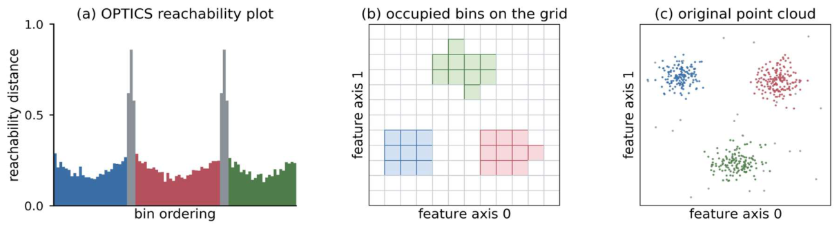
Figure 2.
Generators of the hyperoctahedral group acting on the grid of bins, illustrated on the board with bins numbered in row-major order; colour travels with the bin, so each panel shows where a given bin moves. (a) The original grid ; (b) an axis permutation (), here the transpose; (c) an axis reflection (a sign in ). At these generate .
Figure 2.
Generators of the hyperoctahedral group acting on the grid of bins, illustrated on the board with bins numbered in row-major order; colour travels with the bin, so each panel shows where a given bin moves. (a) The original grid ; (b) an axis permutation (), here the transpose; (c) an axis reflection (a sign in ). At these generate .
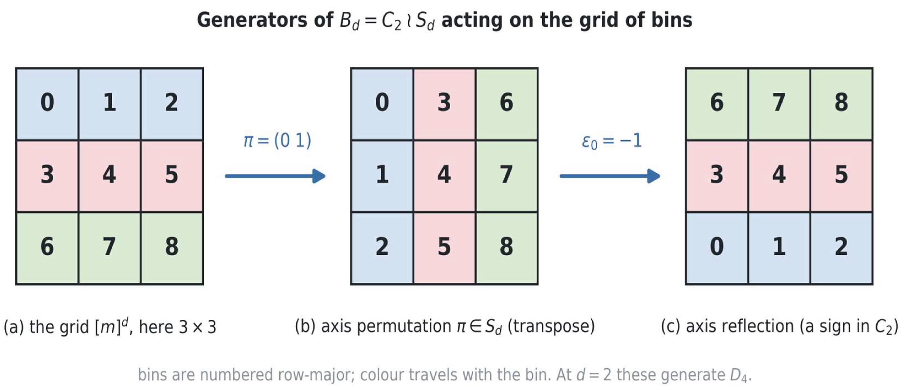
Figure 3.
The equivariance of Theorem 2 as a commuting square: clustering commutes with the group action, .
Figure 3.
The equivariance of Theorem 2 as a commuting square: clustering commutes with the group action, .
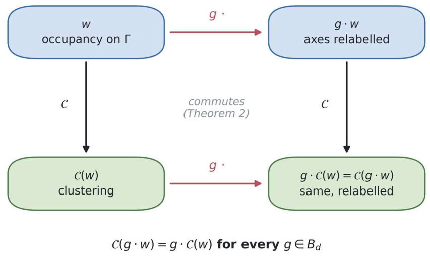
Figure 4.
Growth of the Burnside orbit count (solid) against the raw count (dotted), log scale. As grows the ratio of raw count to orbit count, shown in the inset, approaches .
Figure 4.
Growth of the Burnside orbit count (solid) against the raw count (dotted), log scale. As grows the ratio of raw count to orbit count, shown in the inset, approaches .
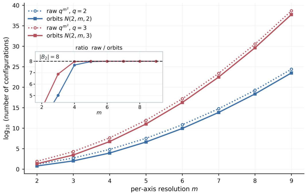
Figure 5.
Orbit-size distribution of acting on binary occupancy functions. (a) At , the orbits split as of size , of size , of size and of size ; (b) at , the orbits are spread over sizes to . As the grid and alphabet grow, the full-size orbits ( ) come to dominate, which is the finite-grid shadow of Proposition 2.
Figure 5.
Orbit-size distribution of acting on binary occupancy functions. (a) At , the orbits split as of size , of size , of size and of size ; (b) at , the orbits are spread over sizes to . As the grid and alphabet grow, the full-size orbits ( ) come to dominate, which is the finite-grid shadow of Proposition 2.
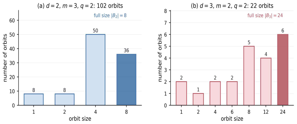
Figure 6.
(a) Fraction of random occupancy functions with non-trivial stabiliser, which falls toward zero as the alphabet grows—generic instances have full-size orbits. (b) What canonicalisation adds over hashing the occupancy function itself, measured on 20,000 independently drawn instances. The additional deduplication factor falls to 1.00 once the instance space is large relative to the workload, so the bound of 8.00 attained by a deliberately closed library (dashed) is not approached by chance.
Figure 6.
(a) Fraction of random occupancy functions with non-trivial stabiliser, which falls toward zero as the alphabet grows—generic instances have full-size orbits. (b) What canonicalisation adds over hashing the occupancy function itself, measured on 20,000 independently drawn instances. The additional deduplication factor falls to 1.00 once the instance space is large relative to the workload, so the bound of 8.00 attained by a deliberately closed library (dashed) is not approached by chance.
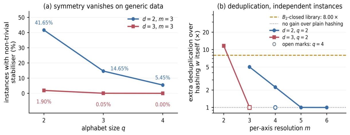
Figure 7.
Where the canonical form sits in a grid-clustering pipeline. Points are binned into an occupancy function, the occupancy function is canonicalised, and the canonical form is used as a cache or index key; by Theorem 2 the clustering computed on the canonical form transfers back to the original grid by relabelling alone.
Figure 7.
Where the canonical form sits in a grid-clustering pipeline. Points are binned into an occupancy function, the occupancy function is canonicalised, and the canonical form is used as a cache or index key; by Theorem 2 the clustering computed on the canonical form transfers back to the original grid by relabelling alone.
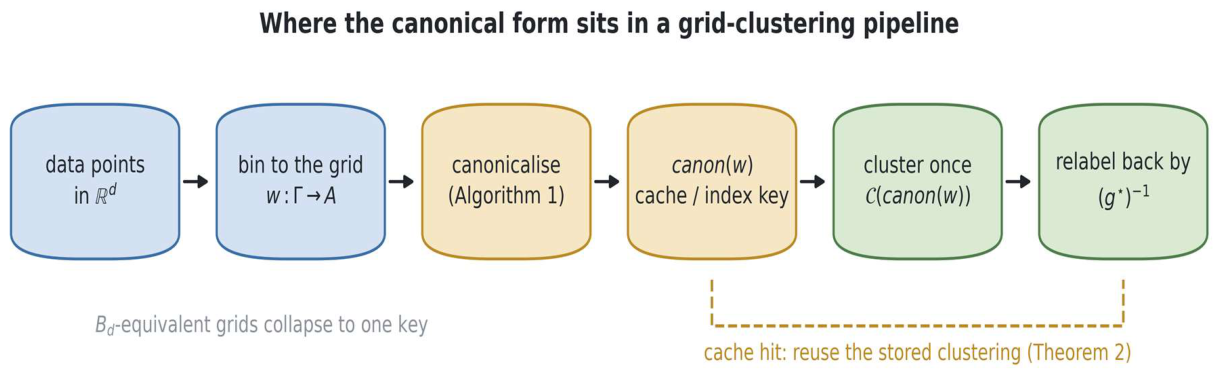
Figure 8.
The subgroup lattice of : the ten subgroups of , ordered by inclusion, which are the candidate stabilisers of a two-dimensional occupancy pattern. The trivial subgroup at the bottom is the generic case (full-size orbit); the whole group at the top corresponds to fully symmetric patterns such as the empty or uniformly full grid.
Figure 8.
The subgroup lattice of : the ten subgroups of , ordered by inclusion, which are the candidate stabilisers of a two-dimensional occupancy pattern. The trivial subgroup at the bottom is the generic case (full-size orbit); the whole group at the top corresponds to fully symmetric patterns such as the empty or uniformly full grid.
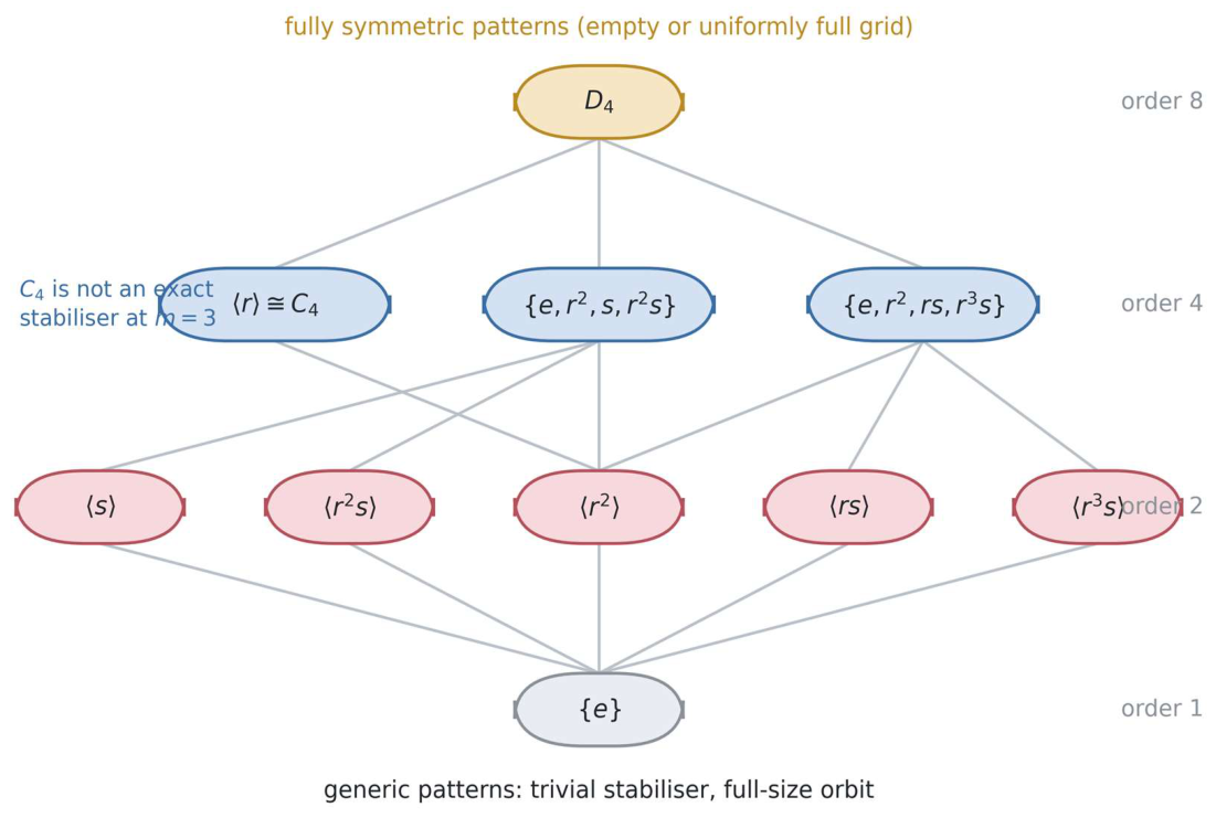

Table 1.
Grid-based and density-based clustering methods to which the analysis applies. In every case the output is a function of bin occupancy and grid adjacency alone, which is what the -model keeps.
Table 1.
Grid-based and density-based clustering methods to which the analysis applies. In every case the output is a function of bin occupancy and grid adjacency alone, which is what the -model keeps.
| Method | Density rule | Grid | Retained by our model |
| DBSCAN [1] | -neighbourhood, minPts | optional (index) | occupancy + adjacency after binning |
| OPTICS [2] | reachability ordering | optional (index) | occupancy + adjacency after binning |
| HDBSCAN [15] | hierarchy of density levels | optional | occupancy + adjacency per level |
| GDBSCAN [17] | generalised neighbourhood | space partition | occupancy + adjacency |
| FlowGrid [3] | bin counts and bin adjacency | equal-width, explicit | exactly the model |
| FLOPTICS [4,5,6] | OPTICS over non-empty bins | equal-width, explicit | the model, at a fixed extraction level |
Table 2.
The present work in relation to prior applications of lattice and hyperoctahedral symmetry.
Table 2.
The present work in relation to prior applications of lattice and hyperoctahedral symmetry.
| Work | Object acted on | Group | Purpose |
| Cycle index of [33,34] | hypercube vertices | classical cycle-index formulas | |
| Lattice-square designs [28] | field-element words | hyperoctahedral dihedral | count non-isomorphic designs |
| Polyomino classes [29] | square-lattice polyominoes | count congruence/rotation classes | |
| -polytopes [30] | cube vertices | classify by vertex count | |
| Canonical labelling [31,32] | graphs / molecules | full automorphism group | isomorphism, deduplication |
| 2D DR Code [12,13] | recoverable layouts | compress a finite catalogue | |
| 3D DR Code [14] | recoverable layouts | compress a finite catalogue | |
| This work | bin-occupancy functions on | canonical indexing, equivariance |
Table 3.
Summary of notation.
| Symbol | Meaning |
| number of feature axes (grid dimension) | |
| per-axis resolution (bins per axis) | |
| grid of bins, | |
| Chebyshev (king-move) bin adjacency | |
| occupancy alphabet and its size | |
| occupancy function | |
| hyperoctahedral group, order | |
| signed permutation (axes signs ) | |
| clustering (partition of dense bins) | |
| density threshold | |
| number of cycles of on the bins | |
| number of occupancy classes up to | |
| lexicographically minimal orbit representative |
Table 4.
The hyperoctahedral group in low dimensions and its identification with the geometric symmetry groups of the DR Code.
Table 4.
The hyperoctahedral group in low dimensions and its identification with the geometric symmetry groups of the DR Code.
| Dimension | Group | Order | Geometric name | DR Code grid |
|---|---|---|---|---|
| 1 | 2 | reflection | — | |
| 2 | 8 | (square) | (2D DR Code) | |
| 3 | 48 | (cube) | (3D DR Code) | |
| 4 | 384 | — | ||
| 5 | 3,840 | — |
Table 5.
Number of bin-occupancy configurations up to , , computed by the Burnside formula of Theorem 3 and confirmed by exhaustive orbit enumeration where the raw space is enumerable. The raw column is .
Table 5.
Number of bin-occupancy configurations up to , , computed by the Burnside formula of Theorem 3 and confirmed by exhaustive orbit enumeration where the raw space is enumerable. The raw column is .
| Raw | Orbits | Ratio | |||
|---|---|---|---|---|---|
| 2 | 3 | 2 | 512 | 102 | 5.02 |
| 2 | 3 | 3 | 19,683 | 2,862 | 6.88 |
| 2 | 4 | 2 | 65,536 | 8,548 | 7.67 |
| 3 | 2 | 2 | 256 | 22 | 11.64 |
| 3 | 3 | 2 | 134,217,728 | 2,852,288 | 47.06 |
| 3 | 3 | 3 | 158,942,078,604 | 47.98 |
Table 6.
The six orbits of acting on binary occupancy functions of the grid (patterns written row-major). Orbit sizes sum to ; the number of orbits is .
Table 6.
The six orbits of acting on binary occupancy functions of the grid (patterns written row-major). Orbit sizes sum to ; the number of orbits is .
| Canonical pattern | Occupied bins | Geometric type | Orbit size | Stabiliser order |
| 0000 | 0 | empty grid | 1 | 8 |
| 0001 | 1 | single corner bin | 4 | 2 |
| 0011 | 2 | two bins on an edge | 4 | 2 |
| 0110 | 2 | two bins on a diagonal | 2 | 4 |
| 0111 | 3 | L-tromino | 4 | 2 |
| 1111 | 4 | full grid | 1 | 8 |
Table 7.
Cost of the canonical-form algorithm (Theorem 5) in the low dimensions relevant to grid clustering. The group size is independent of the data.
Table 7.
Cost of the canonical-form algorithm (Theorem 5) in the low dimensions relevant to grid clustering. The group size is independent of the data.
| Dimension | Push-forwards per instance | Time | Space | |
| 2 | 8 | 8 | ||
| 3 | 48 | 48 | ||
| 4 | 384 | 384 | ||
| general |
Table 8.
Where the symmetry framework helps and where it does not. “Symmetry-closed” means the workload contains complete -orbits of instances.
Table 8.
Where the symmetry framework helps and where it does not. “Symmetry-closed” means the workload contains complete -orbits of instances.
| Setting | Symmetry present? | Benefit | Mechanism |
| Single generic dataset | No (trivial stabiliser) | none | orbit has full size; nothing to collapse |
| Axis-augmented benchmark suite | Yes (closed) | fewer runs/storage | canonical-form deduplication |
| Re-analysis, different axis order | Partial | reuse of cached results | canonical-form cache key |
| Instance registry / audit log | Presentation-only | stable equivalence key | canonical form as identifier |
| Reproducible axis handling | Always | deterministic output | canonical axis order (Theorem 2) |
Disclaimer/Publisher’s Note: The statements, opinions and data contained in all publications are solely those of the individual author(s) and contributor(s) and not of MDPI and/or the editor(s). MDPI and/or the editor(s) disclaim responsibility for any injury to people or property resulting from any ideas, methods, instructions or products referred to in the content. |
© 2026 by the authors. Licensee MDPI, Basel, Switzerland. This article is an open access article distributed under the terms and conditions of the Creative Commons Attribution (CC BY) license.
Copyright: This open access article is published under a Creative Commons CC BY 4.0 license, which permit the free download, distribution, and reuse, provided that the author and preprint are cited in any reuse.