
Submitted:
13 August 2026
Posted:
14 August 2026
You are already at the latest version
Abstract
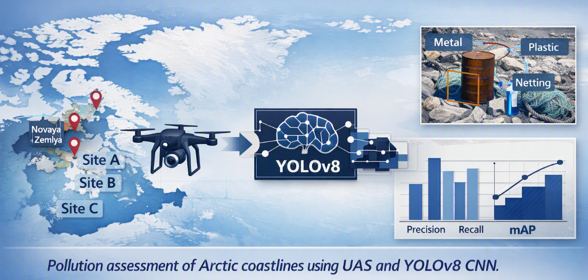
Pollution of coastal territories by marine litter is a pressing issue not only for large cities but also for remote and uninhabited regions such as the Arctic. At the same time, the scale of pollution is growing annually, while existing environmental monitoring methods remain labour-intensive. For the first time, an assessment of the volume and composition of marine litter was conducted for Arctic coastlines using high-resolution airphotos. The method is based on training the YOLOv8 (2023) convolutional neural network in the OBB configuration to recognise plastic, metal, fishing nets, wood, and other types of marine litter in images. Based on a comparative analysis, it was established that machine learning methods combined with remote sensing data represent a new high-precision tool for environmental monitoring, which can significantly contribute to reducing the anthropogenic pressure on the ecosystems of Arctic territories.
Keywords:
unmanned aerial system (UAS)
; deep learning
; marine litter
; plastic
; environmental monitoring
; marine coastline
; convolutional neural network (CNN)
1. Introduction
The Arctic has significant economic, transportation, and industrial potential due to its reserves of natural resources, including hydrocarbons, minerals, biological resources, and renewable energy sources, which are of great strategic importance to the global economy. In particular, the Arctic zone of the Russian Federation (AZRF) is a key center of the country's mineral resource complex and at the same time represents a unique natural environment, especially vulnerable in the context of industrial development of territories. Recently, Arctic ecosystems have been increasingly exposed to man-made impacts due to the active development of mineral deposits in the far north, which requires the development of new, environmentally sound models for the development of the region [1,2]. The melting of ice and permafrost in the Arctic, caused by rapid climate change, not only damages biological diversity, but also causes serious risks of accidents at industrial facilities [3]. In order to ensure environmental safety in the Arctic zone, various monitoring systems have been implemented, but the speed of obtaining data is often limited by the inaccessibility of the territories of the far north and harsh natural and climatic conditions such as permafrost, snow and ice cover.
Remote sensing technologies, which have been actively developing since the middle of the last century and adapted to various environmental protection tasks, have become a reliable tool for environmental monitoring. In the Arctic, unmanned aerial systems (UAS) have successfully proven themselves for monitoring the man-made transformation of the natural environment during the development and operation of fields [4,5], after which UAS have been actively used to control the activities of oil industry facilities, especially in oil spills in the waters [6]. Reliable assessment of the degree of restoration of disturbed lands and compliance with the requirements for reclamation is ensured due to the continuity of satellite survey data. The spatial resolution of modern spacecraft reaches values less than 1 m, which makes it possible to determine with high accuracy the contour change of man-made objects, such as tailings dumps or rock dumps [7]. In addition, due to the coverage of large areas, satellite imagery technologies have become an indispensable tool for monitoring changes in the state of forests [8] and monitoring green spaces in major cities [9]. The experience of the presented studies indicates a high prospect of using remote sensing data in environmental monitoring in the Russian Arctic.
Along with the increase in the facilities of the mineral resource complex and the associated threats to ecosystems from man-made interference, marine pollution, especially pollution of water areas and coastal territories, has become a new challenge for the Arctic region [10]. According to the United Nations Environment Programme (UNEP), marine debris is any persistent, produced or recycled solid material released into the marine and coastal environment [11]. A study of the composition of household waste on the coasts revealed that the largest part of it is plastic of various types and fishing gear, including fishing nets. A separate problem for the Russian part of the Arctic is the objects of accumulated damage - metal barrels stored there for decades [12]. Decomposition products of materials, which are formed under the influence of weather conditions and mechanical deformations, enter the environment, often causing irreparable harm to the ecosystems of the Arctic. An example is microplastics (plastic particles less than 5 mm) accumulating in ice [13].
So, for a new type of pollution, it is necessary to develop a new type of monitoring. Marine debris monitoring is carried out by the Russian Hydrometeorological University, including in the territories of the Arctic zone as part of scientific research expeditions [14]. An important advantage of manual monitoring is, firstly, the ability to accurately determine the type of material and its origin, and secondly, a wide range of sizes of objects. However, in modern conditions, pollution of coastal territories is taking on a new scale, where the efficiency of monitoring is coming to the fore to cover large areas of territory. The disadvantage of the manual monitoring method is the high labor cost and the inability to visually assess the spatial distribution of pollution, as well as to determine the area of large objects.
Therefore, there is an increase in research on the automation of monitoring marine debris on the water surface and on the coasts through the use of remote sensing data and machine learning (MO) [15]. Hyperspectral imaging in the NIR-SWIR range (900-1700 nm) is also a promising direction, which makes it possible to effectively distinguish types of polymers by their spectral reflective characteristics [16]. The possibilities of using such technologies for monitoring pollution of water bodies have been largely considered in the works of foreign scientists [17,18,19].
There is much less research in this area in Russia. The successful experience of integrating remote sensing data with neural network analysis was presented within the framework of the Clean Shore Project. It helps environmental control services and volunteers simplify waste collection on coastal areas [20]. It is worth noting that, for all its advantages, the proposed technology is not adapted to the specifics of the Arctic region. Arctic coasts are a complex environment: objects are small relative to the frame, backgrounds change depending on lighting and weather, and many non-target objects (wood, rocks, algae) visually look like garbage. These difficulties highlight the need to develop reliable methods based on data analysis. For Arctic conditions, scientists at the Moscow Institute of Physics and Technology and the Institute of Oceanology of the Russian Academy of Sciences have developed an artificial intelligence-based system capable of identifying marine debris, as well as birds, glare on the water, and drops on the lens based on images from a camera mounted on a ship [21]. However, this system cannot be effectively used to monitor arctic coasts using images obtained from unmanned aircraft systems.
In order to develop an alternative approach to environmental monitoring in the Arctic, aerial photography of three coasts was conducted for the first time in 2023 as part of the expedition of the Arctic Floating University (AFU). The obtained materials were used to train a convolutional neural network to recognize various types of marine debris. The main limitation in machine learning is the lack of training data, which is why the authors have created their own dataset containing all the man-made objects present in the images. Thus, the aim of the study is to assess the pollution of the Arctic coasts using the YOLOv8 convolutional neural network based on aerial photography. The article describes the main stages of data preparation, dataset creation, model development and training, evaluates the reliability of the model and provides an analysis of errors in the design of marine debris. The accuracy of detecting marine debris from aerial photographs was 80%, which is comparable to the results obtained using other machine learning architectures in the task of detecting marine debris (Random Forest, Support Vector Machine, Naïve Bayes, etc.) [15].
2. Materials and Methods
2.1. Manual Collection and Classification of Marine Litter on Arctic Coastlines
The coastlines of the Novaya Zemlya archipelago are a site of regular monitoring of marine macrolitter in the Barents Sea region as part of expeditions of the Arctic Floating University. During the AFU expedition from 23 June to 15 July 2023, the marine litter monitoring team carried out three landings on Severny Island of the Novaya Zemlya archipelago: at Russkaya Harbour, Cape Zhelaniya and Ledyanaya Harbour. Seven polygons with a length of 100 m each were successively surveyed. Beach surveys were carried out in accordance with the international methodology and recommendations of the OSPAR North-Atlantic region and the AMAP Arctic Monitoring and Assessment Programme [22], which involve manual collection and classification of marine macrolitter (>2.5 cm). The collected marine litter was divided into categories (plastic, metal, glass, rubber, etc.) according to the MSFD classifier [23], counted, and recorded in a protocol.
2.2. General Description of the Marine Litter Detection Methodology on Aerial Images
In order to improve the accuracy and efficiency of monitoring, an automated technique for the identification and classification of marine litter using machine learning was implemented for the first time in this area. At the first stage, a survey of the coastal territory was conducted using an UAS, resulting in a series of aerial images acquired at different flight altitudes. Subsequently, photogrammetric processing of the obtained images was performed to generate a digital surface model and orthophotos of the study site. This step is necessary to eliminate the processing of the same image area due to image overlap [24].
To address the task of marine litter detection in the images, the YOLOv8 (2023) convolutional neural network was selected, which has demonstrated high performance in the field of digital image processing. Training was conducted in the Python language. After training, a final model was obtained, which, for a new orthophoto, outputs the coordinates of bounding boxes where plastic or other types of litter are presumably located, the confidence level for each detection, and the class name. At the final stage, the reliability of the model performance is assessed and error analysis is performed using specialised performance metrics. Thus, the methodology implemented within this study includes the steps presented in Figure 1.
2.3. Conducting Aerial Survey of the Coastlines and Photogrammetric Processing of Aerial Images
In parallel with the manual collection of marine litter during the AFU 2023 expedition, an aerial survey of the studied coastlines was conducted. The survey, using a DJI Mavic Air 2 quadcopter, was carried out for three coastlines of the Novaya Zemlya archipelago: Russkaya Harbour (RG), Ledyanaya Harbour (LG), and Cape Zhelaniya on both the Barents Sea and Kara Sea sides. The obtained high-resolution images (1,039 images) were used for model training. For subsequent analysis of the spatial distribution of anthropogenic objects based on the aerial survey data, photogrammetric processing of the images was performed using the Agisoft Metashape Professional software. Detailed information on the survey and the construction of orthophotos of the area is presented in the authors' previous paper [25].
2.4. Manual Image Screening and Selection of Object Classes
At the next stage, the authors performed manual image screening (visual interpretation) of all images acquired during the survey. Based on the results, all anthropogenic objects were manually counted and recorded in protocols with the assignment of the corresponding class. This method proved to be labour-intensive and fairly subjective; therefore, it was decided to optimise the process and reduce the influence of operator error through automated image processing using machine learning [25].
Based on the results of the preliminary data analysis, it was established that the main pollutants on the Arctic coastlines are plastic, metal, fishing nets, and wood, which were assigned to the corresponding classes. The category "Other debris" included objects whose number was too small to be classified as a separate class, as well as poorly identifiable items. Information on the classes is presented in Table 1.
2.5. Selection of the Machine Learning Model
To select a machine learning model, a review of the scientific literature was conducted, based on which it was established that the most effective supervised learning methods are Random Forest (classification accuracy 92–95%) and Support Vector Machine (89–93%), while the most effective unsupervised learning method is K-means (82.2%). A comprehensive scientific review of this field is presented in the authors' paper [15]. The aforementioned algorithms have been previously used for satellite image processing. A new stage in machine learning is deep learning, specifically the use of convolutional neural networks for object detection in images. CNNs are a specialised class of artificial neural networks designed for processing data with a spatial structure, such as images and video. All modern object detection algorithms can be divided into two broad categories: two-stage detectors and one-stage detectors. One-stage models are characterised by high inference speed and architectural simplicity, which makes them the preferred choice for the task at hand [26].
One of the most widespread one-stage CNNs is YOLO (You Only Look Once) – a family of one-stage object detectors that process an image in a single pass through a convolutional neural network. To date, several versions of YOLO have been developed [27]. Within the framework of this study, the YOLOv8 (2023) model was selected in the OBB (Oriented Bounding Box) configuration. OBB allows for more accurate description of objects located at arbitrary angles to the image axes, as it includes a rotation angle and 8 coordinates of the labelled rectangles instead of 4 [28].
2.6. Data Labelling and Dataset Preparation
In order to address the task of anthropogenic pollution detection in images, several foreign studies have prepared datasets containing images of marine litter on various surfaces: underwater [29], on the water surface [30], on a white surface [31], on land and coastlines [32]. The developed datasets are not applicable within the framework of this study for the following reasons:
- Different flight altitudes,
- Absence of typical pollution objects for Arctic territories (e.g., metal drums and fishing nets),
- The underlying surface of the coastlines differs from the Arctic one (sand instead of the pebbles and large stones characteristic of the Arctic).
In this regard, it was decided to prepare our own dataset, unique to the conditions of Arctic coastlines. To create our own dataset, the Label Studio data labelling and annotation system was used. The initial data consisted of image patches from the orthophotos obtained at the previous stage. Dataset labelling was performed manually. The minimum object size distinguishable in the airphoto was 10 cm. A separate annotation was created for each object, while for overlapping objects only the visible part was labelled, and anthropogenic objects not assigned to any class were classified as "Other". The main difficulties encountered during data labelling were related to:
- Overlapping of objects (e.g., fishing net on a metal drum),
- Complex non-linear shape of objects (fishing nets),
- Inability to determine the object type from the airphoto,
- Uneven stitching of orthophotos.
The total number of labelled objects is 1,973, with 1,039 labelled images, indicating a low density of objects in the airphotos. This feature is characteristic of marine litter datasets and is a major problem in model training [33]. Class imbalance was also identified: the smallest number of objects was in the "Wood" class (15.9%), and the largest in the "Metal" class (34.1%). To address this shortcoming, built-in geometric, compositional, colour, and special augmentations of YOLOv8 OBB were used (image rotation, horizontal and vertical flipping, image scaling, image mosaicking, etc.) [34]. The distribution diagram of the number of objects by class is presented in Figure 2.
After the completion of labelling, the data were exported in the YOLOv8 OBB (TXT) format, where each bounding box is described by a set of parameters: x, y, w, h, θ (x, y – object centre coordinates, w, h – box dimensions, θ – rotation angle relative to the horizontal axis). Subsequently, for model training, the original images of 4000×3000 pixels were resized to the YOLO library format – squares of 1024×1024 pixels in JPEG – using the SAHI library.
2.7. Model Training
To train the model, the original dataset was divided into three subsets: training set, validation set, and testing area. The dataset was split using two approaches – random split and domain shift split. In the first approach, 1,039 images were randomly divided in a 70/20/10 proportion: 727, 208, and 104 images for train, val, and test, respectively. In the second approach, the same proportion yielded 651, 284, and 104 images, respectively. This approach simulates a situation where the model is trained on certain survey areas (e.g., Russkaya Harbour) and tested on others (e.g., Cape Zhelaniya, Ledyanaya Harbour). The main model parameters were: number of epochs: 120, input image size: 1024, batch size: 8, early stopping: after 50 epochs.
AdamW was used as the optimizer. The choice of the AdamW optimizer was driven by its key advantages in the context of sparse experimental data and limited sample size. The adaptive mechanism for adjusting the learning rate for each parameter enables efficient handling of heterogeneous data, while the separate correction of L2 regularisation helps improve the model's generalisation ability and reduce the risk of overfitting. An additional argument is AdamW's robustness to the choice of initial learning rate, which simplifies the hyperparameter tuning process compared to alternative methods.
3. Results
3.1. Training Dynamics
A comparative analysis of the training dynamics under different data split types revealed strong differences. Under the random split, a rapid increase in mAP50 was observed during the first 40 epochs, followed by a slowdown and plateau after 70 epochs. The validation loss decreased synchronously with the training loss, with no overfitting observed. Under the domain shift split, the training dynamics were completely different: the model did not achieve an acceptable level of accuracy, with key performance metrics fluctuating and showing no sustained growth. By the end of training, the metrics declined. At the same time, the training loss continued to decrease, while the validation loss increased – such a divergence is a classic sign of overfitting (Figure 3 and Figure 4).
3.2. Visualisation of Results
After training, a final model was obtained, which for a new image outputs:
- The coordinates of bounding boxes where plastic is presumably located;
- The confidence level for each detection;
- The class of the identified object.
3.3. Model Performance Assessment
To assess the quality of the model performance, the following performance metrics were used: precision, recall, mAP50, and mAP50-95. Precision is the proportion of correctly detected objects among all objects identified by the model. Recall is the proportion of correctly detected objects among all actually existing target objects. mAP (mean Average Precision) is the average precision averaged over all classes. The priority metric is recall, since within the framework of this study, in the context of Arctic territories, missing actual litter causes greater environmental damage than a false positive detection. The criteria for evaluating the success of the experiment were: mAP50 ≥ 0.65, mAP50-95 ≥ 0.35, precision ≥ 0.70, recall ≥ 0.55 [35]. The results of the model performance on the validation and testing sets are presented in Table 2 and Table 3, and on the domain-shifted split in Table 4.
Based on the analysis of the model performance results, it was established that the difficulty of detecting different classes varies. Metallic litter is recognised by the model with the highest efficiency, which is explained by the large volume of the training set and distinctive visual features: all metallic objects have a similar brownish-metallic hue and a clear, well-recognisable geometric shape. Plastic litter (bottles, bags, boxes) demonstrates high detection accuracy due to bright colouration and is well recognised by the model; however, the variety of shapes and shades complicates detection. Fishing gears (nets, ropes, cords) are more difficult for the model to recognise due to the heterogeneity of their structure (tangled shape), but bright colours aid in their detection. The "Other debris" category shows low detection quality: the model misses about half of the objects in this class, which is explained by the internal heterogeneity of the "Other debris" class, which includes visually dissimilar litter items that do not fall into the remaining four categories. Wood (planks, boxes, driftwood) is recognised with the worst performance across all metrics due to visual similarity to natural objects.
3.4. Error Analysis of Model Performance
At the final stage, the model predictions were compared with the original annotations, and each object was classified by error type: FN (False Negative – missed object), FP (False Positive – false alarm), WrongClass – incorrect classification. Table 5 presents the distribution of errors by type committed by the model. The distribution of errors by class is shown in Table 6.
The confusion matrix is presented in Figure 7.
Analysis of the model performance results on the validation set showed that there was virtually no confusion between classes (WrongClass accounted for only 6% of the total number of errors). According to the confusion matrix, the most frequent examples of confusion were fishing gears being mistaken for metal, metal for plastic, and metal for wood. However, the major error occurred precisely in object detection (FN and FP together accounted for 94%), rather than in assigning it to a particular class. The highest number of misses was characteristic of the "Other debris" class, indicating the need either to subdivide objects within this class into additional categories or to expand the training set. At the same time, the model rarely made errors by misclassifying extraneous objects as "Other debris", but often missed actual objects of this category. The largest total number of errors for the "Metal" class correlated with the greatest diversity of the training set; however, the model performance assessment showed a high degree of detection of this class in the airphotos.
4. Discussion
The results of automated detection of marine debris on aerial photographs using machine learning. The study was the first to perform automated detection of marine debris on Arctic coasts using the YOLOv8-OBB convolutional neural network. It was established that the main limitation when working with aerial photographs is the detection threshold, which depends on the flight altitude. In this study, the minimum size of an identified item during airphoto labelling was 10 cm at a flight altitude of 20 m and 40 cm at a flight altitude of 40 m. In addition to the size, the possibility of detecting marine debris is influenced by the color and shape of the object: with a bright contrast with the background and a clear geometric shape, the object is more likely to be identified. For example, the best detection results are typical for the Metal (mAP50 = 0.811) and Plastic (mAP50 = 0.789) classes, while the most challenging classes to recognise were Wood (mAP50 = 0.551) and Other debris (mAP50 = 0.556).
Domain shift. In the course of the work, the risk of such a phenomenon as a domain shift was noted, in which statistical patterns identified by the model on one subset of data lose their significance for another. The domain shift is due to the heterogeneity of the initial data: despite the fact that the survey was conducted in the same area, the studied areas have different types of background, such as pebbles, sand, water, and were taken from different heights (20, 50, 100 m). This paper presents the results of processing images of all coasts, without dividing into separate territories, which was necessary for training the model. As a result, the model may perform worse on other parts of the coast with new shooting parameters. To minimize the domain shift, further research assumes the use of data augmentation with simulation of various shooting conditions (changes in height, illumination, and background type), followed by further training of the model and evaluation of its generalizing ability on independent test sets.
Qualitative assessment of pollution of the coasts of the Novaya Zemlya archipelago based on monitoring results. Monitoring of the coastlines of the Novaya Zemlya archipelago has been carried out for several years, while the composition and quantity of marine debris varies depending on the coast. Thus, in 2021, the predominance of fishing nets and plastic was recorded on the Barents Sea coast, metal - objects of accumulated damage – are largely found on the site from the Kara Sea. Plastic garbage, including fishing nets, fish crates and other fishing vessel waste, was found on Bell Island, while household garbage and other types of materials were practically absent [36]. In 2023, the largest amount of marine debris was detected in the Russian Harbor and Cape Zhelaniya from the Barents Sea, the smallest on the coast of the Ice Harbor. On average, as in previous years, the density of marine debris is higher on the Barents Sea side of the archipelago. The predominance of a small fraction (<50 cm) is noted for almost all coasts. Among the most common finds are fragments and trimmings of fishing nets, parts of fish crates, fastening tapes, pieces of ropes and ropes, as well as various plastic containers (buckets, baskets, bottles of cleaning products and food containers), lids, cartridges and small fragments of plastic [25].
Comparison of marine litter monitoring methods. During this study, pollution assessment of the coastlines was conducted using three different methods:
- Manual collection and classification of marine litter (on 100-m transects);
- Manual screening of UAS images and manual counting of marine litter in the airphotos (for the entire coastline);
- Automated detection and counting of marine litter using the YOLOv8 convolutional neural network (for the entire coastline).
A significant advantage of the manual monitoring method is the ability to identify objects of any size, including small items (<2.5 cm), and in some cases to determine their origin. A comparative analysis showed that the number of objects identified through manual collection significantly exceeds the data obtained by manual image screening and machine learning [25]. However, the manual method has limitations, as it is applied to selected 100-m transects, whereas aerial survey covers the entire shoreline.
As for the methods of processing aerial photographs, manual image screening is a rather labour-intensive process and is characterised by a high degree of subjectivity: an object in the image may be missed by the operator or incorrectly assigned to a class. The use of machine learning methods makes it possible to automate object detection and minimise the number of errors through multi-stage model training. Thus, given the inaccessibility of Arctic territories, the remote sensing method provides an advantage in terms of understanding the overall amount of litter washed ashore and accumulated waste, while the use of machine learning methods makes it possible to optimize the process.
Directions for future work. Future research will focus on the integration of multispectral satellite imagery, hyperspectral survey from a manned vessel, and UAS-based airphotos for the purpose of remote environmental monitoring of coastal territories in the Arctic Zone of the Russian Federation. To address this task, the authors are developing a specialised index for detecting pollution of coastal areas using the spectral signatures of the most common object types. As part of the continued work on machine learning, it is planned to expand the range of objects identifiable by the model by including additional classes in the training set, such as petroleum products and other industrial waste, as well as increasing the dataset to improve the detection accuracy of Wood and Other debris classes.
5. Conclusions
During the study, automated detection of marine debris on the Arctic coasts was performed based on aerial photography data using the YOLOv8 convolutional neural network in a modification for rotated objects (Oriented Bounding Box). The use of the OBB configuration made it possible to identify rotated objects, which is characteristic of marine litter deposits on coastlines. To develop a model adapted to Arctic conditions, a unique dataset has been created, including 1039 aerial photographs of the coasts of the Novaya Zemlya archipelago (waters of the Russian Harbor, Cape of Desire and Ice Harbor) and 1973 annotated objects of five classes.: "Fishing_gear", "Metal", "Other debris", "Plastic" and "Wood". This approach ensures the effectiveness of the model for detecting marine debris in the Arctic.
Training the YOLOv8 model on 727 images, followed by validation on 208 images, allowed us to achieve the following results: average accuracy (Precision) was 0.757, completeness (Recall) was 0.632, and the mAP50 index reached 0.692. The best detection results were recorded for classes Metal (mAP50 = 0.811) and Plastic (mAP50 = 0.789), which is explained by their largest volume in the training sample and their characteristic visual features. The most difficult classes to recognize are "Wood" (mAP50 = 0.551) and "Other debris" (mAP50 = 0.556), which is due to the lack of training data and the high variety of object types within the class. Error analysis showed a balanced distribution of false positives (FP) and missing objects (FN) — 47% of the total number of errors each. The "Other debris" class is characterized by a maximum percentage of omissions (35 FN), which indicates the need to reconsider the expediency of maintaining this category or collecting additional data.
The results of the detection of marine debris from the images allow us to draw the following conclusions about the spatial distribution and composition of waste on the Arctic coasts:
- The structure of the discovered marine debris is dominated by objects of the Metal (673 objects, 34.1% of the total) and Plastic (396 objects, 20.1%) classes, which is consistent with the data of field observations conducted as part of expeditions of the Arctic Floating University. Fishing gear also makes up a significant proportion (Fishing_gear — 315 objects, 16.0%).
- The analysis of the spatial distribution of the detected objects showed the uneven nature of pollution of the studied coasts. The highest density of waste is typical for Cape Zhelaniya from the Barents Sea. The lowest pollution density was noted for the coast of the Ice Harbor, which is due to its greater distance from the main transport routes and less intense anthropogenic impact.
A comparison of different methods of marine debris monitoring has shown that manual collection provides the most detailed information about the qualitative composition of pollution, and the data obtained can be used to verify remote sensing data, however, beach surveys are conducted only at individual landfills with a length of 100 m. Taking pictures from an unmanned aircraft allows you to cover heavy areas of the coast, but detecting marine debris from aerial photographs requires an automated approach, since simply viewing images is labor-intensive and subjective. The proposed method, while yielding to manual collection in the accuracy of identification of small objects, provides automated processing of large amounts of data.
The most effective monitoring tool today remains the combination of manual examination with remote sensing technologies. New data processing technologies provide a visual representation of the types, size, number and spatial distribution of coastal pollution objects such as plastic, metal, building materials, etc., and the manual method remains indispensable for data verification. Thus, in the context of the ever-increasing anthropogenic pressure on aquatic ecosystems, it is critically important to make environmental monitoring of coastal territories not only mandatory, but also optimized.
Further research will be aimed at minimizing the impact of the domain shift by expanding the training sample through the use of data augmentation methods, including variations in shooting height, illumination angle, and background spectral characteristics, as well as using domain adaptation techniques such as Fine-Tuning a pre-trained model based on data from new coast sites. It is planned to validate the trained model on independent test sets formed from snapshots of conditions that are not included in the training and validation samples. In addition, it is planned to expand the list of identifiable classes by including additional categories of man-made objects in the training sample, such as petroleum products and other industrial waste, as well as integrating multispectral and hyperspectral survey data to increase the accuracy of material identification.
Author Contributions
Conceptualization, A.D.; methodology, A.D.; software, E.S.; validation, A.D. and A.E.; formal analysis, A.D.; investigation, E.S.; resources, A.E.; data curation, E.S.; writing—original draft preparation, E.S.; writing—review and editing, A.D. and A.E.; visualization, E.S.; supervision, A.D. and A.E.; project administration, A.D. and A.E.; funding acquisition, A.D. All authors have read and agreed to the published version of the manuscript.
Funding
The work was carried out under the state assignment of the Ministry of Science and Higher Education of the Russian Federation (FSRW-2024-0005).
Institutional Review Board Statement
Not applicable.
Informed Consent Statement
Not applicable.
Data Availability Statement
The datasets presented in this article are not readily available because the data are part of an ongoing study. Requests to access the datasets should be directed to serdukovaelizaveta489@gmail.com.
Acknowledgments
Field data was collected in frames of Arctic Floating University project.
Conflicts of Interest
The authors declare no conflicts of interest. The funders had no role in the design of the study; in the collection, analyses, or interpretation of data; in the writing of the manuscript; or in the decision to publish the results.
Abbreviations
The following abbreviations are used in this manuscript:
| UAS | Unmanned aerial system |
| CNN | Convolutional neural network |
| AZRF | Arctic zone of the Russian Federation |
| UNEP | United Nations Environment Programme |
| MO | Machine learning |
| AFU | Arctic Floating University |
| RG | Russkaya Harbour |
| LG | Ledyanaya Harbour |
| YOLO | You Only Look Once |
| OBB | Oriented Bounding Box |
| mAP | mean Average Precision |
| FN | False Negative |
| FP | False Positive |
References
- Lipina, S.; Zaikov, K.; Lipina, A.V.; Kuprikov, N.; Tsvetkova, A. Roadmaps of Environmental Safety of Promising Coal Deposits in Far North Regions. Int. J. Eng. 2026, 39, 576–584. [Google Scholar] [CrossRef]
- Nikiforov, A.A.; Nikiforova, V.D.; Aksenova, Z.H.A.; Rodionov, D.; Kompaniitseva, O.; Makarenko, E. Energy and infrastructural development of the arctic regions of the Russian federation. Edelweiss Appl. Sci. Technol. 2025, 9, 1186–1195. [Google Scholar] [CrossRef]
- Nevskaya, M.; Belyaev, V.; Aleshichev, S.; Vinogradova, V.; Shagidulina, D. Data Systematization and Preliminary Analysis of Accidental Oil and Petroleum Product Spills in the Russian Arctic and Far North. Resources 2025, 14, 147. [Google Scholar] [CrossRef]
- Buzmakov, S.A.; Sannikov, P.Y.; Kuchin, L.S.; Igoscheva, E.A.; Abdulmanova, I.F. The use of unmanned aerial photography for interpreting the technogenic transformation of the natural environment during the oilfield operation. J. Min. Inst. 2023, 260, 180–193. [Google Scholar] [CrossRef]
- Kazantseva, V.V.; Ozhigin, D.S.; Kosarev, N.S.; Satbergenova, A.K.; Ozhigina, S.B. Development of complex system of geotechnical monitoring of technogenic objects based on geospatial data. J. Min. Inst. 2025, 276, 142–156. [Google Scholar]
- Khalturin, A.A.; Parfenchik, K.D.; Shpenst, V.A. Features of Oil Spills Monitoring on the Water Surface by the Russian Federation in the Arctic Region. J. Mar. Sci. Eng. 2023, 11, 111. [Google Scholar] [CrossRef]
- Kiryushina, E.V.; Zenkov, I.V.; Trinh, L.H.; Dmitrieva, M.L.; Yuronen, Yu.P.; Vokin, V.; Cherepanov, E.V.; Raevich, K.V.; Latyntsev, A.A.; Pavlova, P.L.; Kuzina, L.; Lunev, A.S.; Shtresler, К. Environmental studies of disturbed lands after coal mine closure on sites of the Moscow region coal basin in the Tula region. Ugol 2024, 7, 91–95. [Google Scholar] [CrossRef]
- Nguyen, A.; Kovyazin, V.; Chi Kong, P. Application of Remote Sensing and GIS in Monitoring Forest Cover Changes in Vietnam Based on Natural Zonin. Land 2025, 14, 1037. [Google Scholar] [CrossRef]
- Skachkova, M. E.; Guryeva, O. Monitoring of the State of Saint Petersburg Green Spaces by Remote Sensing Data. Ecol. Ind. Russ. 2023, 27, 51–57. [Google Scholar] [CrossRef]
- Marye, A.T.; Caramiello, C.; De Nardi, D.; Miglino, D.; Proietti, G.; Saddi, K.C.; Biscarini, C.; Manfreda, S.; Poggi, M.; Tauro, F. Remote Sensing for Monitoring Macroplastics in Rivers: A Review. WIREs Water 2025, 12, e70020. [Google Scholar] [CrossRef]
- Morskoy musor | UNEP - UN Environment Programme. Available online: https://www.unep.org/ru/issleduyte-temy/okeany-i-morya/nasha-deyatelnost/rabota-po-regionalnym-moryam/morskoy-musor# (accessed on 17 July 2026).
- Netsvetaeva, O. Marine Beach Litter Monitoring in the Russian Arctic. Ecol. Saf. Coast. Shelf Zones Sea 2022, 4, 69–78. [Google Scholar]
- Mojiri, A.; Zhou, J. L.; KarimiDermani, B.; Vakili, M.; Rezania, S. Microplastics in aquatic environments: Bridging occurrence and mitigation through machine learning detection and bioremediation strategies. Int. Biodeterior. Biodegrad. 2026, 206, 106194. [Google Scholar] [CrossRef]
- Kosinova, A.A.; Ershova, A.I.; Vorotnichenko, E.; Gordeeva, S.; Ruzhnikova, N.; Trofimova, A. Beach litter composition, distribution patterns and annual budgets on Novaya Zemlya archipelago, Russian Arctic. Mar. Pollut. Bull. 2024, 204, 116517. [Google Scholar] [CrossRef] [PubMed]
- Danilov, A.; Serdiukova, E. Review of Methods for Automatic Plastic Detection in Water Areas Using Satellite Images and Machine Learning. Sensors 2024, 24, 5089. [Google Scholar] [CrossRef] [PubMed]
- Alboody, A.; Vandenbroucke, N.; Porebski, A.; Sawan, R.; Viudes, F.; Doyen, P.; Amara, R. A New Remote Hyperspectral Imaging System Embedded on an Unmanned Aquatic Drone for the Detection and Identification of Floating Plastic Litter Using Machine Learning. Remote Sens. 2023, 15, 3455. [Google Scholar] [CrossRef]
- Gonçalves, G.; Andriolo, U.; Pinto, L.; Duarte, D. Mapping marine litter with Unmanned Aerial Systems: A showcase comparison among manual image screening and machine learning techniques. Mar. Pollut. Bull. 2020, 155, 111158. [Google Scholar] [CrossRef] [PubMed]
- Jeong, Y.; Shin, J.; Lee, J.; Baek, J.; Schläpfer, D.; Kim, S.; Jeong, J.; Jo, Y. A Study on the Monitoring of Floating Marine Macro-Litter Using a Multi-Spectral Sensor and Classification Based on Deep Learning. Remote Sens. 2024, 16, 4347. [Google Scholar] [CrossRef]
- Maharjan, N.; Miyazaki, H.; Pati, B.M.; Dailey, M.N.; Shrestha, S.; Nakamura, T. Detection of River Plastic Using UAV Sensor Data and Deep Learning. Remote Sens. 2022, 14, 3049. [Google Scholar] [CrossRef]
- How neural networks help plan coastal cleanups. Available online: https://yandex.cloud/en/special/ai-uborka (accessed on 4 June 2026).
- Bilousova, O.; Krinitskiy, M.; Pogojeva, M.; Spirina, V.; Krivoshlyk, P.N. A Comparison of Self-Supervised and Supervised Deep Learning Approaches in Floating Marine Litter and Other Types of Sea-Surface Anomalies Detection. Remote Sens. 2026, 18, 241. [Google Scholar] [CrossRef]
- Farmen, E.; Provencher, J.; Aliani, S.; Baak, J.; Bergmann, M.; Booth, A.; Bourdages, M.; Buhl-Mortensen, L.; Feld, L.; Gabrielsen, G.; et al. Litter and Microplastics Monitoring Guidelines. Arctic Monitoring & Assessment Programme (AMAP) Version 1.0. 2021. [Google Scholar] [CrossRef]
- Galgani, F.; Ruiz-Orejón, L.; Ronchi, F.; Tallec, K.; Fischer, E.; Matiddi, M.; Anastasopoulou, A.; Andresmaa, E.; Angiolillo, M.; Bakker, M.; et al. Guidance on the Monitoring of Marine Litter in European Seas. 2023. [Google Scholar] [CrossRef]
- Bryn, M.Y.; Mustafin, M.G.; Bashirova, D.R.; Vasilev, B.Y. Investigation of the accuracy of constructing digital elevation models of technogenic massifs based on satellite coordinate determinations. J. Min. Inst. 2025, 271, 95–107. [Google Scholar]
- Ershova, A.A.; Golubeva, E.A.; Antonov, E.V.; Serdiukova, E.A. Comparison of results of ground-based and remote (UAV) methods of marine debris monitoring on the coast of the Novaya Zemlya archipelago in 2023. J. Hydrometeorol. Ecol. 2025, 81, 699–717. [Google Scholar]
- Biliškov, I.; Papic, V. Development of a Seafloor Litter Database and Application of Image Preprocessing Techniques for UAV-Based Detection of Seafloor Objects. Electronics 2024, 13, 3524. [Google Scholar] [CrossRef]
- Zhai, X.; Huang, Z.; Li, T.; Liu, hanzheng; Wang, S. YOLO-Drone: An Optimized YOLOv8 Network for Tiny UAV Object Detection. Electronics 2023, 12, 3664. [Google Scholar] [CrossRef]
- Li, X.; Tian, M.; Kong, S.; Wu, L.; Yu, J. A modified YOLOv3 detection method for vision-based water surface garbage capture robot. Int. J. Adv. Robot. Syst. 2020, 17, 172988142093271. [Google Scholar] [CrossRef]
- Đuraš, A.; Wolf, B.J.; Ilioudi, A.; Palunko, I.; Bart, D.S. A Dataset for Detection and Segmentation of Underwater Marine Debris in Shallow Waters. Sci. Data. 2024, 11, 921. [Google Scholar] [CrossRef] [PubMed]
- Kikaki, K.; Kakogeorgiou, I.; Mikeli, P.; Raitsos, D.E.; Karantzalos, K. MARIDA: A benchmark for Marine Debris detection from Sentinel-2 remote sensing data. PLoS ONE 2022, 17, 1. [Google Scholar] [CrossRef] [PubMed]
- TrashNet: Dataset of Trash Images // GitHub. Available online: https://github.com/garythung/trashnet (accessed on 15 May 2026).
- TACO: Trash Annotations in Context // TACO Dataset. Available online: http://tacodataset.org (accessed on 15 May 2026).
- Yang, S.; Cheng, H.H.; Yu, C. Real-Time Object Detection and Tracking for Unmanned Aerial Vehicles Based on Convolutional Neural Network. Electronics 2023, 12, 4928. [Google Scholar] [CrossRef]
- Nisa, U.; Pozi, M.S.; Saip, M.A. A systematic image augmentation framework based on dataset limitations for small object detection. Iran. J. Comput. Sci. 2026, Vol. 9.(No. 1. 9). [Google Scholar] [CrossRef]
- Hua, Wei; Chen, Q. A survey of small object detection based on deep learning in aerial images. Artif. Intell. Rev. 2025, 58, 162. [Google Scholar] [CrossRef]
- Vesman, A.; Moulin, E.; Egorova, A.; Zaikov, K. Marine litter pollution on the Northern Island of the Novaya Zemlya archipelago. Mar. Pollut. Bull. 2020, 150, 110671. [Google Scholar] [CrossRef] [PubMed]
Figure 1.
Methodology for marine litter detection from aerial images using machine learning [compiled by the authors].
Figure 1.
Methodology for marine litter detection from aerial images using machine learning [compiled by the authors].
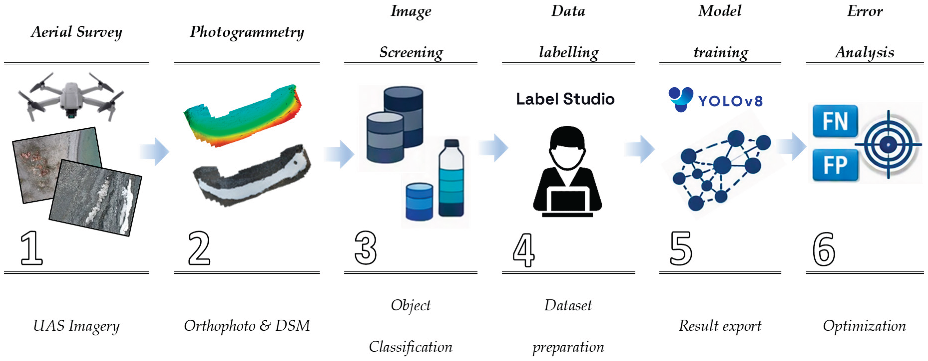
Figure 2.
Distribution of the number of dataset objects by class [compiled by the authors].
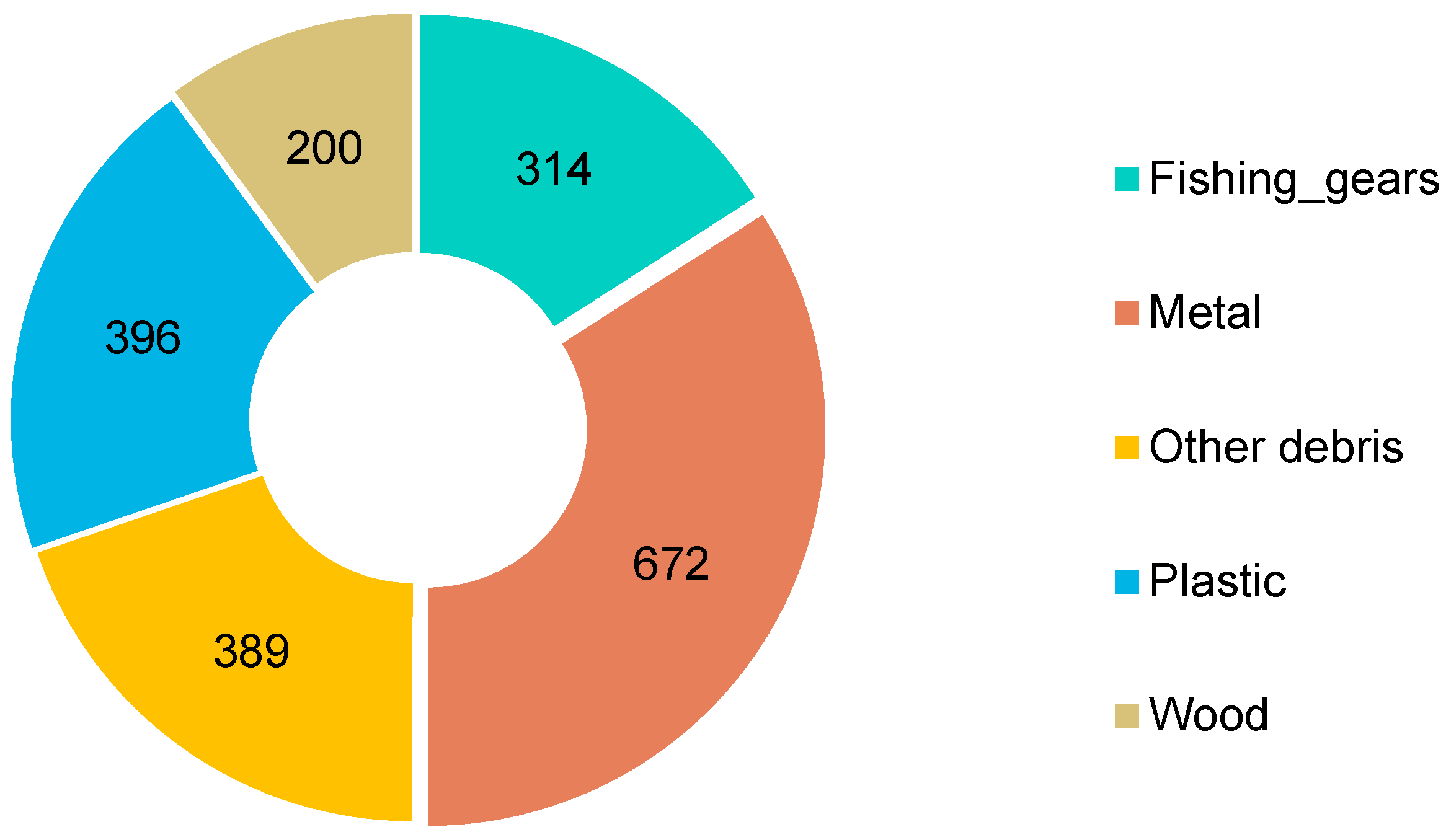
Figure 3.
Differences in training on the two datasets [compiled by the authors].
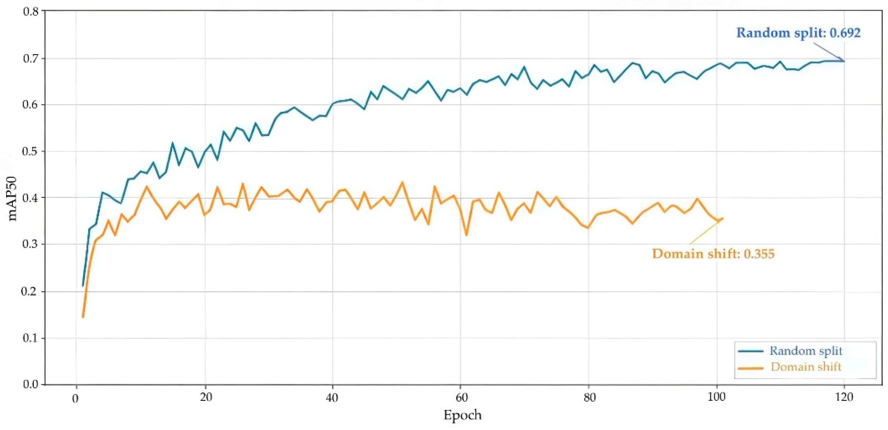
Figure 4.
Training dynamics on the testing and validation sets [compiled by the authors].
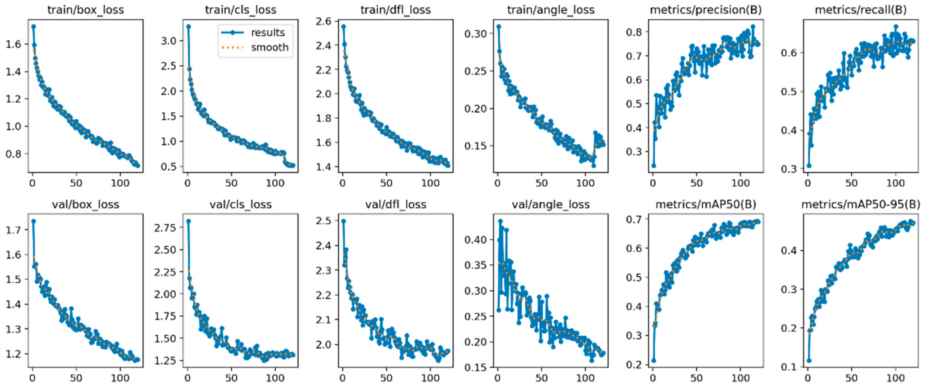
Figure 5.
Example of detection for the "Fishing_gears" and "Plastic" classes [compiled by the authors].
Figure 5.
Example of detection for the "Fishing_gears" and "Plastic" classes [compiled by the authors].
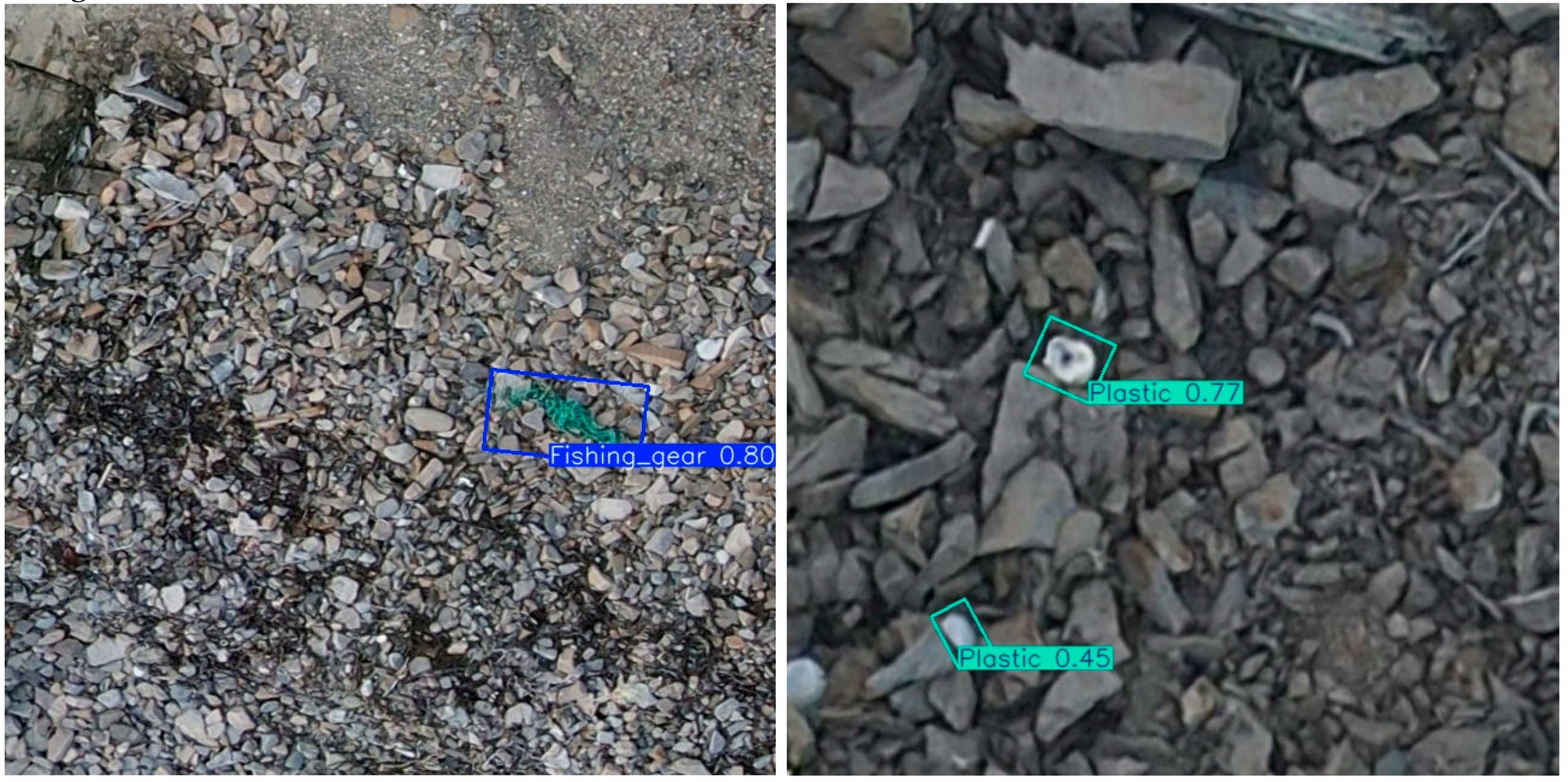
Figure 6.
Example of detection for the "Metal", "Wood", and "Other debris" classes [compiled by the authors].
Figure 6.
Example of detection for the "Metal", "Wood", and "Other debris" classes [compiled by the authors].
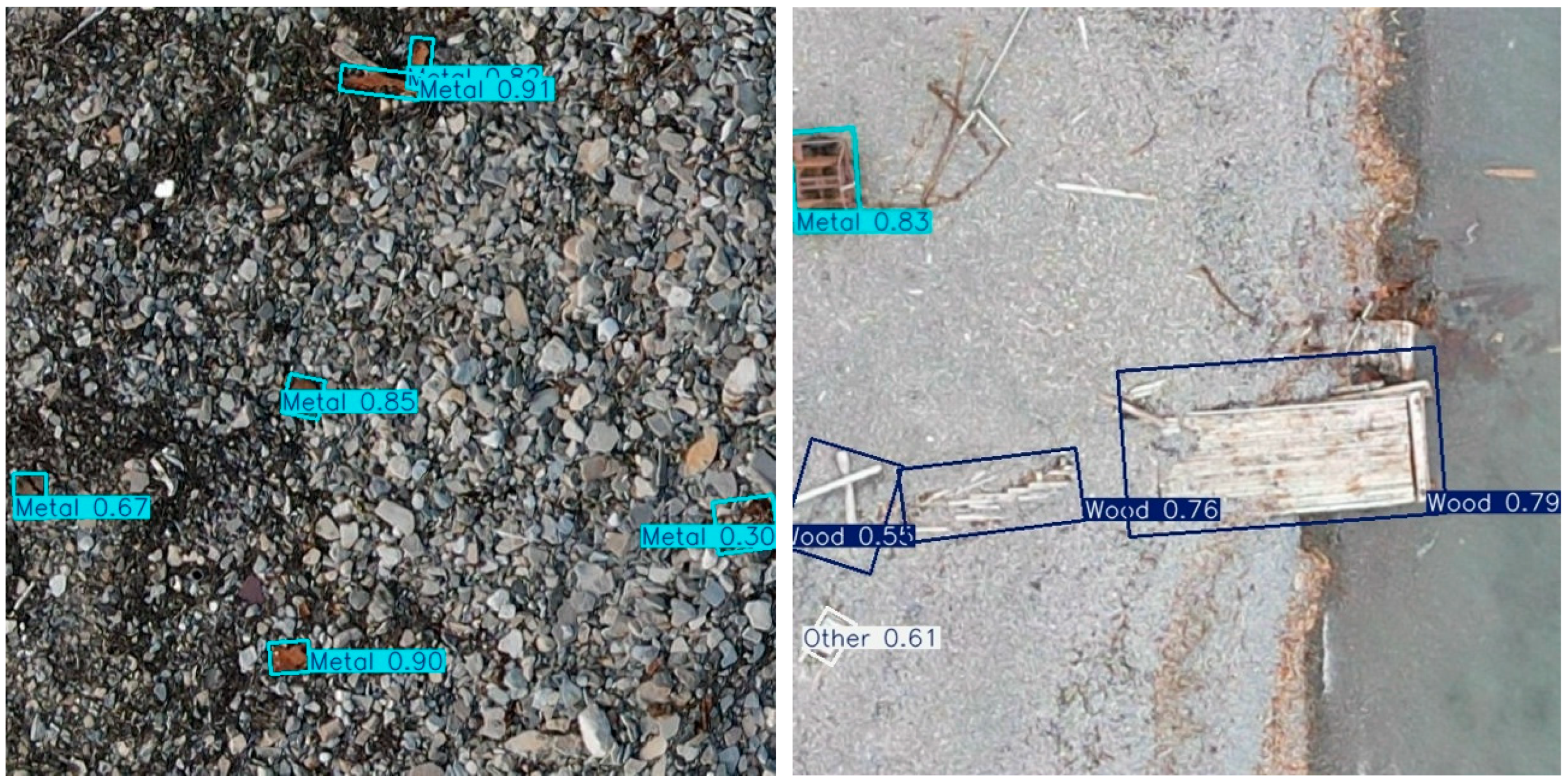
Figure 7.
Confusion matrix [compiled by the authors].
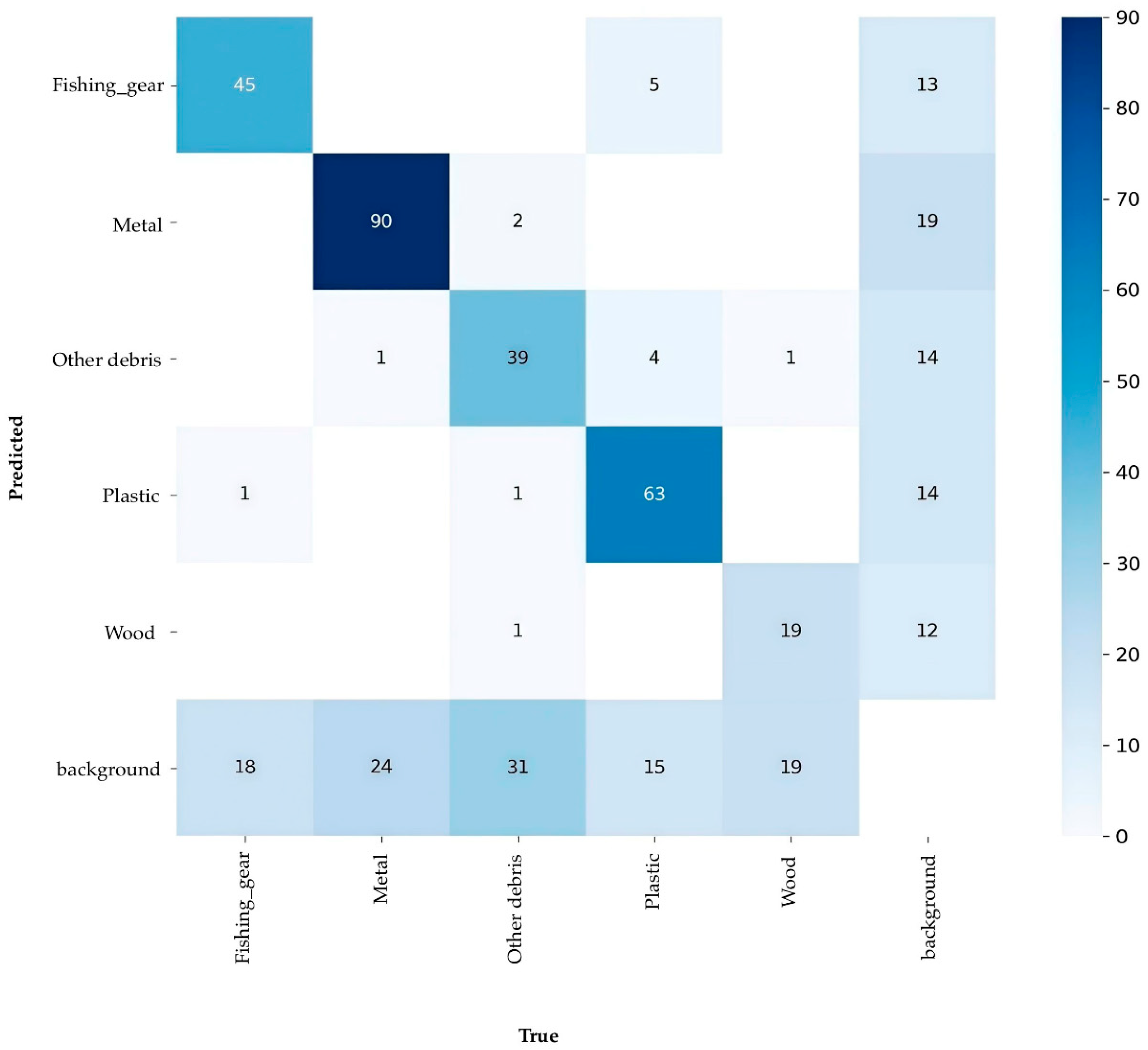

Table 1.
Description of the training set classes [compiled by the authors].
| Class name | Code according to classifier* | Class description | Example image from airphoto |
|---|---|---|---|
| Plastic | J16, J7-9, J18, J80 | Plastic jerry cans / bottles / plastic fish boxes / plastic fragments | 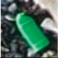 |
| Fishing_gears | J49, J242 | Plastic rope (diameter more than 1 cm) / plastic string and cord (diameter less than 1 cm) | 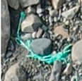 |
| Metal | J187, J186, J199, J198, | Metal drums & barrels / metal industrial scrap / other metal pieces > 50 cm / other metal pieces 2.5 cm – 50 cm | 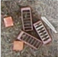 |
| Wood | J164, J160, J162, J172 | Wooden fish boxes / wooden pallets / wooden crates, boxes, baskets for packaging / other processed wooden items (>50 cm) | 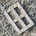 |
| Other debris | J251 | Rubber tyres / unidentifiable or mixed objects / other types of debris | 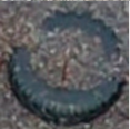 |
*Note: The code is given according to the MSFD classifier (pp. 164–170 of the Appendix to the Guidance on the Monitoring of Marine Litter in European Seas 2023 [23]).
Table 2.
Model performance metrics on the validation set (random split) [compiled by the authors].
| Class | Class ID | Precision | Recall | mAP50 | mAP50-95 |
|---|---|---|---|---|---|
| Fishing_gears | 0 | 0,813 | 0,703 | 0,755 | 0,477 |
| Metal | 1 | 0,803 | 0,757 | 0,811 | 0,573 |
| Other debris | 2 | 0,706 | 0,514 | 0,556 | 0,401 |
| Plastic | 3 | 0,820 | 0,701 | 0,789 | 0,548 |
| Wood | 4 | 0,645 | 0,487 | 0,551 | 0,376 |
| Average | 0,757 | 0,632 | 0,692 | 0,475 |
Table 3.
Model performance metrics on the testing set (random split) [compiled by the authors].
| Class | Class ID | Precision | Recall | mAP50 | mAP50-95 |
|---|---|---|---|---|---|
| Fishing_gears | 0 | 0,915 | 0,520 | 0,630 | 0,419 |
| Metal | 1 | 0,851 | 0,627 | 0,797 | 0,541 |
| Other debris | 2 | 0,907 | 0,522 | 0,636 | 0,510 |
| Plastic | 3 | 0,8700 | 0,632 | 0,763 | 0,573 |
| Wood | 4 | 0,857 | 0,684 | 0,721 | 0,513 |
| Average | 0,88 | 0,597 | 0,709 | 0,511 |
Table 4.
Model performance metrics on the validation set (domain split shift) [compiled by the authors].
Table 4.
Model performance metrics on the validation set (domain split shift) [compiled by the authors].
| Class | Class ID | Precision | Recall | mAP50 | mAP50-95 |
|---|---|---|---|---|---|
| Fishing_gears | 0 | 0,584 | 0,550 | 0,523 | 0,275 |
| Metal | 1 | 0,573 | 0,489 | 0,522 | 0,336 |
| Other debris | 2 | 0,430 | 0,360 | 0,265 | 0,197 |
| Plastic | 3 | 0,593 | 0,481 | 0,514 | 0,354 |
| Wood | 4 | 0,646 | 0,339 | 0,338 | 0,196 |
| Average | 0,565 | 0,444 | 0,432 | 0,272 |
Table 5.
Model errors [compiled by the authors].
| Error type | Number of errors | Share of total errors, % |
|---|---|---|
| FN | 129 | 47 |
| FP | 129 | 47 |
| WrongClass | 15 | 6 |
| Total | 273 | 100 |
Table 6.
Distribution of errors by class [compiled by the authors].
| Class | Class ID | FN | FP | Total errors |
|---|---|---|---|---|
| Fishing_gears | 0 | 19 | 24 | 43 |
| Metal | 1 | 28 | 42 | 70 |
| Other debris | 2 | 35 | 15 | 50 |
| Plastic | 3 | 28 | 30 | 58 |
| Wood | 4 | 19 | 18 | 37 |
Disclaimer/Publisher’s Note: The statements, opinions and data contained in all publications are solely those of the individual author(s) and contributor(s) and not of MDPI and/or the editor(s). MDPI and/or the editor(s) disclaim responsibility for any injury to people or property resulting from any ideas, methods, instructions or products referred to in the content. |
© 2026 by the authors. Licensee MDPI, Basel, Switzerland. This article is an open access article distributed under the terms and conditions of the Creative Commons Attribution (CC BY) license (http://creativecommons.org/licenses/by/4.0/).
Copyright: This open access article is published under a Creative Commons CC BY 4.0 license, which permit the free download, distribution, and reuse, provided that the author and preprint are cited in any reuse.