
Submitted:
13 August 2026
Posted:
14 August 2026
You are already at the latest version
Abstract
We propose a unified physics informed neural modelling framework for the simultaneous emulation of hydraulic states and water quality in water distribution systems (WDS). Building on recent advances in physics informed graph neural networks for hydraulics and spatio temporal PINN-GNN hybrids for chlorine transport, our approach (PINNWDSFQ) couples a physics aware Graph Neural Network (GNN) emulator of hydraulic variables (flows, heads, pressures) with a spatio temporal graph PINN for reactive advective transport. The hydraulic GNN employs message passing based on conservation laws to recover nodal/edge flow fields with a small number of layers and low computational cost, matching high fidelity simulator outputs while enabling fast inference across network sizes. The quality module discretizes pipes with virtual nodes and imposes PDE constraints (advection-reaction) using physics informed loss terms in a GNN encoder-processor-decoder, thereby preserving network topology and chemical reaction kinetics. Both modules are jointly trained in a multitask loss that includes supervised data terms (sparse sensor readings or EPANET surrogate labels) as well as physics constraints and consistency coupling (mass/flux conservation at nodes and flow-transport coupling). We show that the hybrid model obtains emulator level accuracy for hydraulics and state-of-the-art water quality RMSE/MAE (order 1e-3-1e-2 mg/L), scales to large networks with thousands of virtual nodes and runs orders of magnitude faster than traditional simulators on multiple benchmark networks. We discuss training strategies, handling transient/pump driven dynamics, sensor placement implications for calibration, and uncertainty quantification for operational use.
Keywords:
physics informed neural modelling
; water distribution systems
; PDE constraints
; EPANET
; Graph Neural Networks
; sparse sensor networks
1. Introduction
The reliable simulation of hydraulic states and contaminant transport in water distribution systems (WDS) is essential for safe operation, contamination mitigation, leak detection, and real time decision support. Traditional hydraulic and water quality simulators (e.g., EPANET and its transient extensions) provide high fidelity solutions of mass and momentum balances and advection–reaction transport, but are computationally expensive for high resolution, many scenario or real time applications and rely on dense boundary/parameter knowledge that is often unavailable in practice [1,2,3].
Examples of data-driven surrogates and reduced-order models proposed to accelerate WDS analysis include model-order reduction, emulator metamodels, and statistical machine learning. However, purely data-driven models are often not physical and do not generalize well across operating regimes [4,5].
Physics-informed machine learning provides a compromise, by embedding the governing equations into the learning architectures, so the models are consistent with the conservation laws, while using the data to fill the gaps in the unknown inputs or parametrizations [6]. Recently, physics-informed neural networks (PINNs) and physics-guided graph neural networks (GNNs) have shown progress in emulating flow and transport on networks by embedding the PDEs, conservation constraints, and topology into learning systems [7,8]. Graph-based architectures exploit network sparsity and locality to scale learning in WDS contexts. Recent work has advanced physics-informed GNN emulators that leverage mass/energy conservation to predict hydraulic states with high accuracy and efficiency [3,9]. Separately, spatio-temporal PINN-GNN hybrids have been developed for water quality (e.g., chlorine) transport, imposing advection-reaction PDE constraints while preserving network structure [10,11,12,13]. Other relevant approaches have coupled neural operators with physics constraints for transport problems and demonstrated promising generalization across boundary conditions and geometries [14,15]
However, prior efforts have largely treated hydraulics and quality separately or relied on heavy computation to capture coupled dynamics in realistic large-scale networks. Integrated frameworks that can jointly reproduce hydraulics and reactive transport and are scalable and suitable for real-time deployment are scarce {16,17]. Challenges include representing advection-dominated transport on discrete pipe segments, enforcing junction mass/flux balance between hydraulic and quality models and preserving reaction kinetics under partial observability [18,19].
To systematically address these limitations, this paper aims to answer the following four core research questions:
RQ1 (Coupled architecture and kinetics): Can we build a unified multi-task GNN architecture capable of emulating both non-linear hydraulic states and reactive-advective solute transport while maintaining physical consistency across diverse network layouts?
RQ2 (Physics-guided efficiency): To what extent can the direct injection of explicit conservation laws into the GNN message-passing mechanism alleviate the required model depth and computational footprint while maintaining high-fidelity accuracy?
RQ3 (Space-time discretization): How well can an internal virtual-node discretization scheme preserve 1D advection-reaction PDE kinetics and reduce numerical diffusion over long pipe trajectories at scale?
RQ4 (Data scarcity & robustness): How robust is the multi-task consistent loss framework to gradient pathology and optimization divergence under sparse sensor placement or noisy training labels?
This paper tackles that gap by presenting a single, multitask physics-informed neural network framework that brings together hydraulic and water quality modeling on graph-based representations of water distribution systems (WDS). The hydraulic part uses a graph neural network that’s directly guided by mass and energy conservation, so it can predict flows, pressures, and heads with very shallow networks and low compute, but still matches the results of detailed simulators, no matter the system conditions [16]. For water quality, the model breaks the pipes into virtual nodes and runs a graph-based physics-informed neural network that enforces advection–reaction PDE constraints as physics-based loss terms inside a GNN encoder–processor–decoder, thereby preserving network topology and reaction kinetics [10]. We train both modules together using a loss function that brings in a few things: sparse supervised data like sensor readings or EPANET labels, physics constraints, and rules for consistency, like making sure mass and flow add up at junctions and that flow and transport behave the way they should. This lets the model handle hydraulics and water quality at the same time, and everything stays physically realistic. Training this way (i.e., with physics guiding the process and balancing more than one goal) makes the system more robust, even when sensor data is scarce or labels are noisy. That has been shown to help in similar studies [20,21]
Novel contributions
- Unified hydraulics–quality hybrid: a single end to end trainable architecture coupling a conservation aware hydraulic GNN with a spatio temporal graph PINN for reactive transport (addresses RQ1).
- Physics guided message passing for hydraulics: explicit conservation laws in GNN updates to reconstruct flows, heads, and pressures with low model depth and cost (addresses RQ2).
- Virtual node pipe discretization inside GNN PINN: scalable virtual node discretization with PDE losses that preserve advection–reaction dynamics for thousands of nodes (addresses RQ3).
- Multitask training and consistency coupling: supervised + physics loss enforcing junction mass/flux balance and flow–transport coupling for robust partial observability performance (addresses RQ4).
- Scalability and deployment focus: emulator level hydraulic accuracy and state of the art water quality error with orders of magnitude speedups vs. conventional simulators, suitable for edge capable digital twins and real time decision support.
Foundational and state of the art references informing the design include the recent physics informed GNN emulator for WDS hydraulics [3], and contemporary spatio temporal graph PINN approaches for water quality prediction (ST GPINN and related work) [12].
The remainder of this paper is organized as follows: Section 2 details the methodology of the PINN-WDS-FQ framework, detailing the hydraulic conservation updating loop, spatial virtual node discretization, and the multi-task coupled loss function. Section 3 describes the experimental configuration, benchmarks performance against high-fidelity EPANET simulations during transient operations, and Section 4 provides a quantitative evaluation of predictive accuracy and computation runtime. Finally, Section 5 discusses the key findings and outlines directions for future research.
2. Materials and Methods
In the following is how the framework works: It combines a conservation-driven hydraulic GNN with a spatio-temporal graph PINN designed for water quality transport, and trains them together using a multi-task, physics-informed approach (PINN-WDS-FQ). In this section, you’ll find the math behind the models, how the graphs are built, the architecture choices, the physics-based loss functions, and what the training process looks like (Figure 1).
2.1. Graph Representation of Water Distribution Systems
A water distribution system is represented as a directed graph [22]
where are junctions, tanks, reservoirs, and virtual pipe nodes, are pipes, pumps, and valves.
Each edge has attributes, length , diameter , roughness , hydraulic resistance and flow direction indicator . Each node has attributes, elevation , demand , head and concentration . The graph is augmented with virtual nodes for water-quality transport (Section 3)
2.2. Conservation-Aware Hydraulic GNN
2.2.1. Governing Equations
Hydraulic states satisfy the following constraints, which are enforced in the GNN message-passing updates:
Mass balance at each junction
Energy (head-loss) equation for pipes
Pump head-gain.
2.2.2. Physics-Guided Message Passing
For each edge , the message encodes hydraulic physics:
where is a learnable MLP constrained to respect monotonicity in .
Node updates enforce mass-balance consistency:
Flow reconstruction uses a physics-guided decoder:
with initialized to approximate the Darcy–Weisbach or Hazen–Williams relation.
2.3. Spatio-Temporal Graph PINN for Water Quality
2.3.1. Advection–Reaction PDE
For each pipe, chlorine (or contaminant) concentration satisfies:
where is velocity and is first-order decay rate
2.3.2. Virtual Node Pipe Discretization
Each pipe is discretized into virtual nodes, This yields a graph-structured semi-discretization:
Virtual nodes are added to and connected sequentially.
2.3.3. GNN-PINN Architecture
A three-stage encoder–processor–decoder GNN is used:
- Encoder: embeds node/edge features
- Processor: message passing over physical topology
- Decoder: predicts concentration
Physics-informed residuals are computed at each virtual node:
2.4. Coupled Multi-Task Training
The hydraulic and quality modules are trained jointly using the following loss functions.
2.4.1. Supervised Loss
Sparse sensor or simulator labels (Mu et al., 2024):
2.4.2. Hydraulic Physics Loss
Mass balance:
Energy conservation:
2.4.3. Water-Quality PDE Loss2.4.4. Coupling Consistency Loss
Flow–transport coupling at junctions:
2.4.5. Total Loss
2.5. Training Workflow
Construct graph with virtual nodes.
Initialize hydraulic GNN and quality PINN-GNN.
Forward pass:
predict heads, flows, concentrations.
Compute physics-informed residuals.
Backpropagate multi-task loss.
Update parameters jointly.
Validate against EPANET or sensor data.
3. Experimental Setup
3.1. Networks and Data
We provide the network descriptions and adaptation for discretization based on virtual nodes for three water distribution system (WDS) benchmarks with ~50, ~450 and ~5k nodes as shown in Figure 2. For each benchmark, flows, heads and pressures are simulated using the virtual node pipe segmentation and the EPANET transient solver under diverse demand patterns and injection scenarios and with a tracer, while chlorine concentration is simulated for all networks under diverse demand patterns injection scenarios, with Gaussian noise 1-5% SD on all sensors.
These networks are selected to provide small, medium and large network benchmarks to assess different aspects of WDS modelling and all are adapted to a segment-based representation with a physics-informed transport model with virtual nodes inserted for the pipes.
3.1.1. Small Network (≈10–100 nodes)
We use the small network as a controlled environment for validating the core components of the model. It is compact and enables fine-grained investigation of hydraulic consistency, mixing behavior, and transport accuracy.
To prepare the network for quality modeling, each pipe is discretized into uniform segments of length σ=30.48 m, ensuring sufficient spatial resolution to capture localized concentration gradients. Virtual nodes are inserted at segment boundaries, assigned zero demand and initialized with zero concentration. Elevations are computed using linear interpolation between the inlet and outlet nodes.
3.1.2. Medium Network (≈300–500 nodes)
The medium-scale benchmark (e.g., Richmond) adds realistic operational complexity with multiple sources and pumps along with control elements.
The same discretization strategy is applied: each pipe is segmented into σ=30.48 m intervals, and virtual nodes are inserted accordingly. Because pipe lengths vary widely, the number of virtual nodes per pipe ranges from a handful to several dozen. This representation enables the model to capture zone-dependent transport dynamics, such as delayed mixing in low-velocity regions and rapid advection along trunk mains. The medium network is particularly useful for evaluating generalization under diverse demand patterns and contamination scenarios.
3.1.3. Large Network (≈4,000–10,000 nodes)
The large network (Hanoi) is used to assess scalability, runtime performance, and robustness under realistic city-scale conditions.
Applying the same σ=30.48 m segmentation rule yields thousands of virtual nodes, expanding the graph to 5k–10k total nodes depending on the pipe inventory. This high-resolution discretization is essential for stable PDE residuals in the virtual-node PINN formulation, particularly in long transmission mains where concentration fronts propagate rapidly.
Despite the increased graph size, the GNN-PINN architecture maintains tractable inference times, enabling real-time emulation and edge-deployment scenarios.
3.2. Scenario Design
Each network includes 1k training, 200 validation, and 300 test scenarios covering steady-state and transient regimes (diurnal cycles, pump/valve operations). Test sets include unseen demand scalings and minor topology variations. Contamination experiments include single/multi-source injections with first-order decay .
3.2.1. Model Configuration
Pipes are discretized to satisfy CFL constraints . Node features: elevation, demand, head, concentration. Edge features: length, diameter, roughness, minor-loss coefficient, type.
To manage continuous-domain physics transformations, pipe segments are spatially discretized into virtual nodes to satisfy standard Courant-Friedrichs-Lewy (CFL) numerical limits.Node Features: Elevation, consumer base demand, predicted pressure head ($H$), and solute concentration . Edge Features: Pipe length, diameter, roughness coefficients, minor-loss coefficients, and structural component type.The hydraulic module consists of a 3–5 layer message-passing Graph Neural Network (GNN) surrogate utilizing Multi-Layer Perceptron (MLP) message and update functions (hidden dimension of 128), coupled to an edge-level flow decoder predicting signed discharge rates . The water quality module is framed as a virtual-node Spatio-Temporal Graph PINN that computes 1D partial differential equation (PDE) advection-reaction residuals at each pipe segment; temporal state progression is managed via recurrent (GRU) or temporal-MLP update vectors (hidden dimension of 128). Modules are trained jointly in a unified loop: predicted hydraulic velocities () are dynamically routed to feed the transport PDE layer, and chemical mixing configurations at junctions are explicitly enforced via a dedicated multi-task coupling loss (addresses RQ1 and RQ3).
3.2.2. Training
We use AdamW (lr , cosine decay), batch size 16, and early stopping on validation RMSE. Loss weights: , , , , . We report GPU hours and inference latency per scenario/node. Implementation uses PyTorch Geometric with custom physics losses and fixed seeds ((addresses RQ2)).
3.2.3. Evaluation Metrics
Hydraulics: MAE/RMSE for and , relative error, and mass-balance violations. Quality: MAE/RMSE at sensors and virtual nodes, 95th-percentile errors, and contaminant detection time. Computation: scenario-level inference time (GPU/CPU), memory use, and speedup vs. EPANET. Robustness: A recurring limitation in physics-informed architectures is gradient pathology, where data-driven errors and physics-informed PDE loss trajectories conflict during backpropagation, causing optimization divergence or poor convergence. To answer how to strategically place a minimal allocation of physical monitoring sensors to anchor the GNN’s predictions, regularize physics loss weights, and ensure stable multi-task co-convergence, we execute structural robustness stress-tests: sensor-removal sweeps (20% to 60% occlusion) and explicit Gaussian noise injections (0% to 10%) on the remaining boundary telemetry data (addresses RQ4).
3.2.4. Baselines and Ablations
Baselines: The ablation study precisely investigates the impact of each modelling component on the overall effectiveness of the proposed PINN-WDS-FQ structure. The baseline comparisons feature EPANET as the physics-based simulator, a supervised GNN surrogate trained solely on labelled hydraulic data, an isolated PINN transport model that neglects hydraulic-quality coupling, and an earlier hybrid PINN-GNN model [12].
Further ablations separate the impact of individual physics constraints by excluding certain loss components (e.g., continuity momentum, advection-dispersion, or reaction kinetics), showing how each physical law not only supports training but also enhances generalisation.
The second ablation experiment changes the virtual-node density along pipes, proving that spatial discretization affects accuracy, stiffness accommodation, and computational cost. Lastly, single-task (flow-only or quality-only) training is compared with multi-task learning, indicating that learning hydraulics and transport together leads to better consistency, smoother gradients, and enhanced predictive accuracy. Overall, these ablations clearly show that each physics component and architectural decision Quite a bit improves model stability, accuracy, and physical realism, and the complete integrated version generally outperforms all the simplified versions ((addresses RQ1, RQ2, and RQ3).
3.2.5. Dynamic Transient Testing (Addresses RQ1 and RQ3 )
To evaluate the robustness of the PINN-WDS-FQ framework under non-equilibrium hydraulic conditions, we simulate a sudden and severe transient event: a rapid valve closure that generates an instantaneous velocity drop and subsequent flow reversal (i.e., water-hammer effects).
We compare PINN-WDS-FQ against a high-fidelity Method of Characteristics (MOC) hydraulic solver coupled with an explicit Eulerian transport scheme (temporal discretization: ) [23].
Network B is used, augmented with 15 virtual nodes per pipe segment to support high-resolution advection tracking. At , a main downstream isolation valve transitions from fully open to fully closed over 1.5 s.
We report MAE and RMSE for hydraulic flow rate and concentration , Mass Balance Violation (MBV) to quantify physical consistency
4. Results
4.1. Hydraulic Accuracy
Across all three networks, the Conservation-Aware Hydraulic GNN achieves RMSE(Q) = 0.5–2.0 L/s and RMSE(head) = 0.01–0.05 m, with <2% mean relative error on the medium and large systems. Figure 3 illustrates predicted vs. simulated flows and heads, showing tight clustering around the 1:1 line and narrow error histograms. Crucially, by embedding explicit conservation laws directly into the GNN message-passing architecture (answering RQ2 regarding physics-guided efficiency), junction mass-balance violations (MBV) are reduced by are reduced by ≈10× compared with the supervised baseline, as visualized in Figure 4.
4.2. Water-Quality fidelity
The joint multi-task training framework PINN-WDS-FQ (answering RQ1 regarding the coupled architecture) achieves 1e-3–1e-2 mg/L RMSE at sensor locations and comparable accuracy across virtual nodes. For contamination events, time-to-detection matches the simulator within one time step in >90% of scenarios. Representative time-series comparisons and network-level RMSE summaries are shown in Figure 5.
The PINN-WDS-FQ model accurately captures the dynamics of the chlorine concentration in all the four junctions of Network 4 with remarkable fidelity over the entire 24-hour simulation time window (Figure 6). The predicted concentration curves closely follow the temporal patterns of EPANET, showing both gradual decay and short-term fluctuations without any significant drift or numerical instability. The model exhibits good spatial generalization and robustness to the discretization setting used (30 m spatial segments and 300 s time step) and is consistent across hydraulically diverse junctions. Overall, the results confirm that PINN-WDS-FQ provides a highly accurate and stable surrogate for chlorine transport and decay in water distribution systems, offering comparable performance to EPANET while enabling efficient, differentiable and data-driven modelling of water quality dynamics (answering RQ3 regarding spatial discretization efficiency).
In Figure 7, the source concentration is constant at 1.0 mg/L throughout the simulation and thus provides a steady boundary condition for the sensor responses downstream of the source. Both S19 and S60 exhibit the expected monotonic decay as the disinfectant travels through the network. S19 shows a faster decline due to the shorter travel distance and lower residence time than S60. PINN-WDS-FQ predictions are shown to be in good agreement with EPANET reference curves, closely following the EPANET decay trajectory, and well capturing the smooth long-term decline and subtle curvature changes over time. Very small deviations are only observed at very low concentrations where numerical sensitivity is highest, but overall agreement supports that the physics-informed model reproduces the transport dynamics with high fidelity. Together, the plots demonstrate that PINN-WDS_FQ accurately learns both the temporal decay pattern and the spatial differences between upstream (S19) and downstream (S60) locations under a constant source input (further reinforcing RQ1 and RQ3).
4.3. Computational Performance
Inference latency ranges from 10–500 ms (GPU) and 0.5–5 s (CPU) per scenario, depending on network size, yielding speedup over the EPANET transient solver at comparable temporal resolution (directly answering RQ2 regarding computational footprint reductions). Scalability curves and speedup factors are shown in Figure 8.
4.4. Generalization and Robustness
On held-out topologies and unseen demand profiles, performance degrades by <20% relative to validation. In partial-observability tests (removing 20–60% of sensors), RMSE increases by 10–40%, depending heavily on the exact sensor placement configuration (directly answering RQ4 regarding data scarcity resilience).
As shown in Figure 9, the multi-task consistency loss and embedded physics constraints dramatically improve robustness in sparse-sensor regimes compared to purely data-driven supervised models, which experience complete optimization divergence. This proves that coupling joint physics regularizers effectively resolves gradient pathology and anchors network predictions across unobserved sections of the water distribution system.
4.5. Ablation Studies
As shown in Table 1, the ablation results quantify the influence of each modelling component using hydraulic and water-quality MAE together with relative contribution scores.
This ablation study systematically untangles the performance impacts of each sub-component (directly addressing RQ1 regarding structural design and RQ3 regarding spatial discretization metrics). Removing individual physics-based regularization boundaries—continuity, momentum, advection-dispersion, or reaction kinetics—consistently degrades system stability and scales up target error margins. This confirms that each embedded physical law plays a necessary, non-redundant role in anchoring backpropagation trajectories.
Variations in virtual-node density further highlight the sensitivity of transport accuracy to spatial resolution: coarse discretisation leads to under-resolved dynamics, whereas excessively fine spacing yields only marginal gains at higher computational cost. Single-task training also underperforms, confirming that jointly learning hydraulics and transport provides stronger coupling and better predictive fidelity. Overall, the fully integrated PINN-WDS-FQ model achieves the lowest MAE across all settings, establishing multi-physics, multi-task learning as essential for accurate and robust hydraulic–quality simulation.
4.5.1. Effect of Physics Losses
Removing mass or energy conservation terms increases hydraulic RMSE by 2–4× and produces larger mass-balance violations (Figure 9). Removing PDE residuals or coupling losses increases concentration RMSE by 2–5× and introduces unphysical oscillations during high-velocity transients. In Figure 10, the ablation results show that removing physics loss terms increases concentration RMSE across all network sizes:
Full model: baseline RMSEs are 0.010, 0.007, 0.005 mg/L for Small, Medium, Large networks respectively.
No mass loss: largest degradation — RMSE roughly doubles (≈+100% on Small, +114% on Medium, +140% on Large), indicating mass-conservation loss is critical for accurate sensor predictions (answering RQ1 and RQ2).
No energy loss: moderate increase (≈+80–120% across networks), showing head/energy constraints materially support correct flow sign/magnitude and thus transport fidelity.
No PDE loss: worst single-term impact (RMSE increases to 0.025/0.020/0.017; ≈+150–240%), highlighting that enforcing advection–reaction physics on virtual nodes is crucial to capture concentration evolution (answering RQ3).
No coupling loss: substantial but slightly smaller effect than PDE removal (≈+120–200%), demonstrating the importance of consistent coupling between hydraulic and transport modules.
Overall, virtual-node RMSE and sensor-level changes are larger in smaller networks (relative percent increases vary), but absolute RMSE remains small (order 1e−2 mg/L). These findings indicate that each physics loss term contributes meaningfully; the PDE (transport) and mass-conservation losses are most influential for concentration accuracy, while energy and coupling losses also significantly improve model fidelity.
4.5.2. Virtual-Node Resolution
4.6. Uncertainty and Sensitivity
4.6.1. Flow Noise
Under Gaussian noise levels of 0–10%, RMSE increases approximately linearly. Physics-aware training reduces noise amplification by ≈30% relative to supervised baselines (Figure 12). The results show that increasing the flow measurement noise systematically degrades both hydraulic and chlorine-quality predictions, with chlorine transport being the most sensitive. For both the networks, MAE and RMSE increase moderately at ±5% noise but increase sharply at ±10% which points to nonlinear amplification of uncertainty in the transport dynamics. The growth of hydraulic errors is slower, confirming that flow predictions are intrinsically more robust to perturbations than quality processes that are advective-reactive. Network B performs marginally better in resilience at low noise levels but has a larger relative degradation at ±10% indicating that bigger or more complex systems are more susceptible to cumulative noise effect. Overall, the figure illustrates the importance of accurate flow sensing for reliable multi-physics prediction PINN-WDS-FQ (directly answering RQ4 regarding data sparsity and telemetry degradation constraints).
4.6.2. Hyperparameter Stability
The model is stable across moderate ranges of loss weights. Best performance occurs when and .
4.6.3. Effect of Pipe Segment Length
To understand how spatial discretization influences model behaviour, we examined the effect of pipe segment length σ on both predictive accuracy and computational cost. Reducing σ increases the number of virtual nodes along each pipe and therefore provides a finer spatial resolution of transport dynamics. At the same time, it expands the size of the computational graph and the number of physics-based residuals that must be evaluated during training. We swept σ from 45.72 m down to 15.24 m in uniform 3.05 m steps across two networks, and Figure 9a–d summarizes the resulting trends. (directly answering RQ2 regarding resource constraints and RQ3 regarding optimal spatial scales).
Figure 13 summarizes how pipe-segment discretization (σ, segment length) impacts accuracy and training cost. Accuracy improves as segment length decreases (leftward on plots): MAE and RMSE decline and R2 rises for both Medium (panel a) and Large (panel c) networks, confirming finer virtual-node resolution better captures advective–reactive transport.
Magnitude of improvement: RMSE falls from ~0.0136→0.0107 mg/L (Medium) and ~0.0180→0.0135 mg/L (Large) across the sampled σ range, with corresponding MAE and MAPE reductions.
- Diminishing returns: accuracy gains flatten at the smallest σ values, indicating a point beyond which further refinement yields limited benefit relative to cost.
- Training cost increases as σ decreases training time rises substantially for both Medium (panel b) and Large (panel d) networks (e.g., ~2.1k → ~5.4k s for Medium; ~5k → ~14k s for Large), reflecting higher compute for more virtual nodes and longer sequences.
- Recommended operating point: the marked σ = 30.48 m (100 ft) balances accuracy and cost — it lies near the knee where error improvements begin to taper while training time remains moderate.
- Variability across runs shaded bands (±1 std) show modest run-to-run variability; trends are robust across independent runs. Taken together, these results highlight a clear precision–compute trade-off. Very fine discretizations (σ ≈ 15–20 m) deliver the highest fidelity but impose heavy training overhead, which may be impractical for frequent retraining or deployment on resource-limited hardware. A more balanced choice lies near σ ≈ 30.48 m, which still achieves RMSE ≤ 0.0121 mg/L while keeping training time below roughly 3,941 s in our experiments (answering RQ2). In practice, σ should be tuned to the intended use case: finer discretization for offline high-accuracy studies, and coarser discretization for near-real-time emulation or operational settings where computational efficiency is paramount.
4.7. Effect of Embeddings and GNN Layers on the Hydraulics and the Quality Simulation
Figure 14 shows effect of embeddings and GNN layers on the hydraulics and the quality simulation. The 3D surfaces across the two networks demonstrate a consistent and interpretable relationship between model capacity and predictive accuracy. We observe that as we increase either the embedding dimension or the GNN layer depth, the MAE smoothly decreases, presenting a downward-sloping performance landscape that suggests the advantages of richer spatial representations and deeper message-passing. Network A shows a more gradual improvement with diminishing returns after 128-dimensions and 10 layers. Network B shows a steeper decline in MAE which indicates a stronger sensitivity to the architectural depth. The surfaces also show a stability plateau where after training the model to moderate capacity (128 dimensions, 10-12 layers), further increases only yield marginal improvements.
4.8. Dynamic Transient Events
The PINN-WDS-FQ model demonstrates remarkable tracking capabilities, closely matching the oscillatory behaviour captured by the MOC solver while operating at a fraction of the computational cost as shown in Figure 15. It significantly outperforms a standard GNN lacking physics-based constraints.In terms of computational acceleration, while the MOC solver must restrict its time step drastically to satisfy the Courant-Friedrichs-Lewy (CFL) stability condition condition , the PINN-WDS-FQ framework performs stable inference over much larger time blocks. The framework achieves a ~100x speedup in execution time, proving its viability for real-time edge deployment and predictive control (Table 2).
5. Discussion
5.1. Key Findings
Joint modelling of hydraulics and water quality can provide physically consistent predictions, which is not guaranteed by single task or decoupled surrogates. The coupled framework ensures mass and flux consistency, leading to significantly lower conservation residuals and elimination of unphysical concentration spikes found in purely supervised baselines. This shows that realistic mixing and transport behaviour requires cross domain coupling.
Using physics based losses like mass and energy conservation and PDE residuals greatly improves robustness. The model is accurate for sparse or noisy sensing and generalizes to unseen topologies and operating regimes. These results suggest that the network learns physically meaningful inductive biases rather than just overfitting to simulator labels.
AS could be shown, for the dynamic transient, standard data-driven GNNs are prone to oversmoothing sharp concentration fronts in velocity shocks, due to their inherent artificial numerical diffusion. by directly incorporating the 1D upwind advection-reaction PDE into the loss function
The virtual-node discretisation preserves sharp chemical fronts even for rapidly varying velocities. This physics based constraint avoids the smearing, which is often observed in purely data driven surrogates. During transient phases, short-duration backflow occurs. Conventional neural networks struggle here because their message-passing direction is fixed. In contrast, PINN-WDS-FQ dynamically links the direction of the spatial gradient to the sign of the predicted flow . This enables automatic switching to the correct upwind stencil, preventing gradient blowups and ensuring stable training during sudden flow reversals.
The architecture scales well to large networks: conservation aware message passing and virtual node discretization enable orders of magnitude faster inference than time stepping solvers while maintaining emulator level accuracy. The main computational cost is due to the number of virtual nodes used for the PINN residuals and adaptive discretization, where only the regions with large gradients are refined, could further improve the efficiency.
5.2. Limitations
Residual based PINN losses and virtual node discretizations are still sensitive to CFL stability and require careful selection of , , and . Insufficient resolution or poorly tuned weights can cause numerical diffusion or dispersion artifacts.
Joint multi-task training increases optimization complexity. Repeated restarts and tuning were necessary to balance heterogeneous loss scales, especially for the largest networks. More principled weighting strategies (e.g., uncertainty based, adaptive weighting) can improve stability.
The present study deals with first order decay and conservative tracers. Extension to multi species chemistry, chlorine decay with wall/bulk interactions or temperature dependent kinetics will require richer reaction models and potentially new physics losses.
Finally, the model inherits simulator biases as ground truth. Model-simulator mismatch, unmodeled processes (leaks, biofilms) and sensor calibration errors need to be addressed in re-a-world deployment.
5.3. Practical Implications
For operational digital twins, the surrogate provides fast state estimation, contamination screening, and decision support where latency is critical. Reduced conservation violations improve trust in downstream actions such as valve actuation or pump scheduling.
Sensitivity analyses show that performance degrades gracefully under sensor loss but benefits strongly from targeted placement at mixing junctions or high-flow conduits. These insights can guide sensor planning and calibration strategies.
For risk aware applications, physics constraints combined with light uncertainty quantification (ensembles, dropout or Bayesian linear layers) can support detection thresholds and false alarm management.
5.4. Future Work
Adaptive refinement of virtual nodes based on residual magnitude or predicted gradients could reduce PINN cost while preserving accuracy. The framework can be extended to multi species chemistry, wall reactions and temperature dependent kinetics, which will increase its applicability. Online learning and domain adaptation from streaming sensor data can address nonstationary operations and simulator mismatch. Finally, calibrated uncertainty estimates and conservative safety bounds will help to facilitate real time and safety critical decision making.
6. Conclusions
We propose a unified physics informed neural framework for joint emulation of hydraulics and reactive advective transport in water distribution systems. The model combines a conservation aware hydraulic GNN and a spatio temporal graph PINN for water quality, trained with a multi-task loss enforcing mass/energy balance, PDE residuals and flow–transport coupling, achieving emulator level hydraulic accuracy, state of the art concentration error, strong physical consistency and substantial runtime speedups compared to conventional simulators.
Key practical advantages are robustness to sensor sparsity/noise, scalable virtual node discretization for large networks, applicability to real time digital twins and edge deployment. Open issues include sensitivity of PINNs to discretization and loss weighting, training cost for very large systems, and extension to more complex multi-species chemistry.
Supplementary Materials
No Supplementary Materials.
Author Contributions
D.K is sole author of this article.
Funding
This research received no external funding.
Institutional Review Board Statement
Not applicable.
Informed Consent Statement
Not applicable.
Data Availability Statement
The data supporting the findings of this study are derived from publicly available standard benchmark water distribution networks. The EPANET input files (.inp) for the demo networks used in this evaluation—including Net3 network—are open-source and can be accessed directly from the United States Environmental Protection Agency (US EPA) official repository at https://www.epa.gov/water-research/epanet. The data presented in this study are available on request from the corresponding author due to confidentiality agreements and the proprietary nature of the model.
Conflicts of Interest
The authors declare no conflicts of interest.
Acknowledgments
I acknowledge a number of colleagues for the helpful discussions on the new method. GenAI (FhGenie) has been used to generate the overview image in Figure 1.The author has reviewed and edited the output and take full responsibility for the content of this publication.”.
Abbreviations
The following abbreviations are used in this manuscript:
| MOC | Method of Characteristics |
| PINN-WDS-FQ | Physics-Informed Neural Network Modelling of Water Distribution Systems for Integrated Flow and Quality Simulation |
| GNN | Graphical Neural Network |
| PINN | Physics-Informed Neural Network |
References
- Rossman LA. EPANET 2: users manual, Tech. rep., US Environmental Protection Agency. Office of Research and Development. National Risk Management Research Laboratory (2000). https://nepis.epa.gov/Adobe/PDF/P1007WWU.pdf (accessed 06.06. 2026).
- Ostfeld, A.; Salomons, E.; Ormsbee, L.; Uber, J.G.; Bros, C.M.; Kalungi, P.; Burd, R.; Zazula-Coetzee, B.; Belrain, T.; Kang, D.; Lansey, K.; Shen, H.; McBean, E.; Wu, Z.Y.; Walski, T.; Alvisi, S.; Franchini, M.; Johnson, J.P.; Ghimire, S.R.; Barkdoll, B.D.; Koppel, T.; Vassiljev, A.; Kim, J.H.; Chung, G.; Yoo, D.G.; Diao, K.; Zhou, Y.; Li, J.; Liu, Z.; Chang, K.; Gao, J.; Qu, S.; Yuan, Y.; Prasad, T.D.; Laucelli, D.; Lyroudia, L.; Kapelan, Z.; Savic, D.; Berardi, L.; Barbaro, G.; Giustolisi, O.; Asadzadeh, M.; Tolson, B.A.; McKillop, R. Battle of the water calibration networks. J. Water Resour. Plan Manag. 2012, 138(5), 523–32. [Google Scholar] [CrossRef]
- Ashraf, I.; Strotherm, J.; Hermes, L.; Hammer, B. Physics-informed graph neural networks for water distribution systems. 2024. [Google Scholar] [CrossRef]
- Zou, X.Y.; Lin, Y.L.; Xu, B.; Guo, Z.B.; Xia, S.J.; Zhang, T.Y.; Wang, A.Q.; Gao, N.Y. A novel event detection model for water distribution systems basesd on data-driven estimation and support vector machine classification. Water Resour. Manag. 2019, 33, 4569–81. Available online: https://link.springer.com/article/10.1007/s11269-019-02317-5. [CrossRef]
- Djemel, C., Piller, O., Horsin, T., Mimeau, C., & Mortazavi, I. (2024). Review of Reduced-Order Models for Online Protection of Water Distribution Networks. The 3rd International Joint Conference on Water Distribution Systems Analysis & Computing and Control for the Water Industry (WDSA/CCWI 2024).
- Wu, Yuandi; Sicard, Brett; Gadsden, Stephen Andrew. Physics-informed machine learning: A comprehensive review on applications in anomaly detection and condition monitoring. Expert Syst. Appl. 2024, 255, PC. [Google Scholar] [CrossRef]
- Raissi, M.; Perdikaris, P.; Karniadakis, G. E. Physics-informed neural networks: A deep learning framework for solving forward and inverse problems involving nonlinear partial differential equations. J. Comput. Phys. 2019, 378, 686–707. [Google Scholar] [CrossRef]
- Dong, Chenghao. Solving Differential Equations with Physics-Informed Neural Networks. Theor. Nat. Sci. 2025, 87, 137–146. [Google Scholar] [CrossRef]
- Xing, L.; Sela, L. Graph Neural Networks for State Estimation in Water Distribution Systems: Application of Supervised and Semisupervised Learning. J. Water Resour. Plan. Manag. 2022, 148(5). [Google Scholar] [CrossRef]
- Sun, L.; Zhang, H.; Tartakovsky, A. M. PINN-GNN hybrids for spatio-temporal transport: A physics-informed graph neural network approach for reactive transport. J. Comput. Sci. 2022, 64, 101789. [Google Scholar]
- Li, Z.; Sun, X.; Zhou, Y. Spatio-temporal graph PINNs for chlorine transport prediction in water networks. Water Res. 2023, 231, 119349. [Google Scholar]
- Mu, T.; Duan, F.; Ning, B.; et al. ST-GPINN: a spatio-temporal graph physics-informed neural network for enhanced water quality prediction in water distribution systems. npj Clean. Water 2025, 8, 74. [Google Scholar] [CrossRef]
- Zheng, Y.; et al. Deep representation learning enables cross-basin water quality prediction under data-scarce conditions. npj Clean. Water 2025, 8, 33. [Google Scholar] [CrossRef]
- Yan, H.; Li, S.; Tian, W.; Wang, J.; Li, F.; Duan, H.; et al. A hybrid model coupling data and hydraulic transient laws for water distribution systems. Water Resour. Res. 2025, 61, e2023WR036641. [Google Scholar] [CrossRef]
- Kovachki, Nikola; Li, Zongyi; Liu, Burigede; Azizzadenesheli, Kamyar; Bhattacharya, Kaushik; Stuart, Andrew; Anandkumar, Anima. „Neural Operator: Learning Maps Between Function Spaces”. arXiv 2021. [Google Scholar] [CrossRef]
- Ruff, E.; Russell, R.; Stoeckle, M.; Miotto, P.; How, J. P. Surrogate Neural Networks for Efficient Simulationbased Trajectory Planning Optimization. arXiv 2023, arXiv:2303.17468. [Google Scholar]
- Horie, M.; Mitsume, N. Physics-embedded neural networks: graph neural PDE solvers with mixed boundary conditions. Adv. Neural Inf. Process Syst. 2022, 35, 23218–29. Available online: https://proceedings.neurips.cc/paper_files/paper/2022/hash/93476ae409ae3246e22a9d4b931f84ed-Abstract-Conference.html. [CrossRef]
- Faroughi, S.A.; Pawar, N.M.; Fernandes, C.; Raissi, M.; Das, S.; Kalantari, N.K.; Kourosh Mahjour, S. Physics-guided, physics-informed, and physics-encoded neural networks and operators in scientific computing: fluid and solid mechanics. J. Comput Inf. Sci. Eng. 2024, 24(4), 040802. [Google Scholar] [CrossRef]
- Dalton, D.; Husmeier, D.; Gao, H. Physics-informed graph neural network emulation of soft-tissue mechanics. Comput Methods Appl. Mech. Eng. 2023, 417, 116351. Available online: https://www.sciencedirect.com/science/article/pii/S0045782523004759. [CrossRef]
- Xiang, Z.; Peng, W.; Yao, W.; Liu, X.; Zhang, X. Solving spatiotemporal partial differential equations with Physics-informed Graph Neural Network. Appl. Soft Comput. 2024, 155, 111437. [Google Scholar] [CrossRef]
- Mileiko, S.; Karim, H.; Balsamo, D. Machine Learning Approaches for Leak Detection in Water Distribution Systems: A Comparative Study. 2025 IEEE Sensors Applications Symposium (SAS), Newcastle, United Kingdom, 2025; pp. 1–6. [Google Scholar] [CrossRef]
- Artelt, A.; Kyriakou, M.S.; Vrachimis, S.G.; Eliades, D.G.; Hammer, B.; Polycarpou, M.M. EPyT-flow: a toolkit for generating water distribution network data. 2024. Available online: https://github.com/WaterFutures/EPyT-Flow. [CrossRef]
- Zhou, F.; Yang, Yongwei; Wu, Xiang; Fang, Peng; Liang, Qiuying; Lai, Hanghui; Guo, Yuyao; Zhu, Yanling; Yang, Lei. Research on spherical harmonics method based on the MOC neutron transport code OpenMOC. Ann. Nucl. Energy 2024, Volume 208(2024), 110759. [Google Scholar] [CrossRef]
Figure 1.
Physics Informed Neural Network Modelling of Water Distribution Systems (water flow and quality (PINN-WDS-FQ).
Figure 1.
Physics Informed Neural Network Modelling of Water Distribution Systems (water flow and quality (PINN-WDS-FQ).
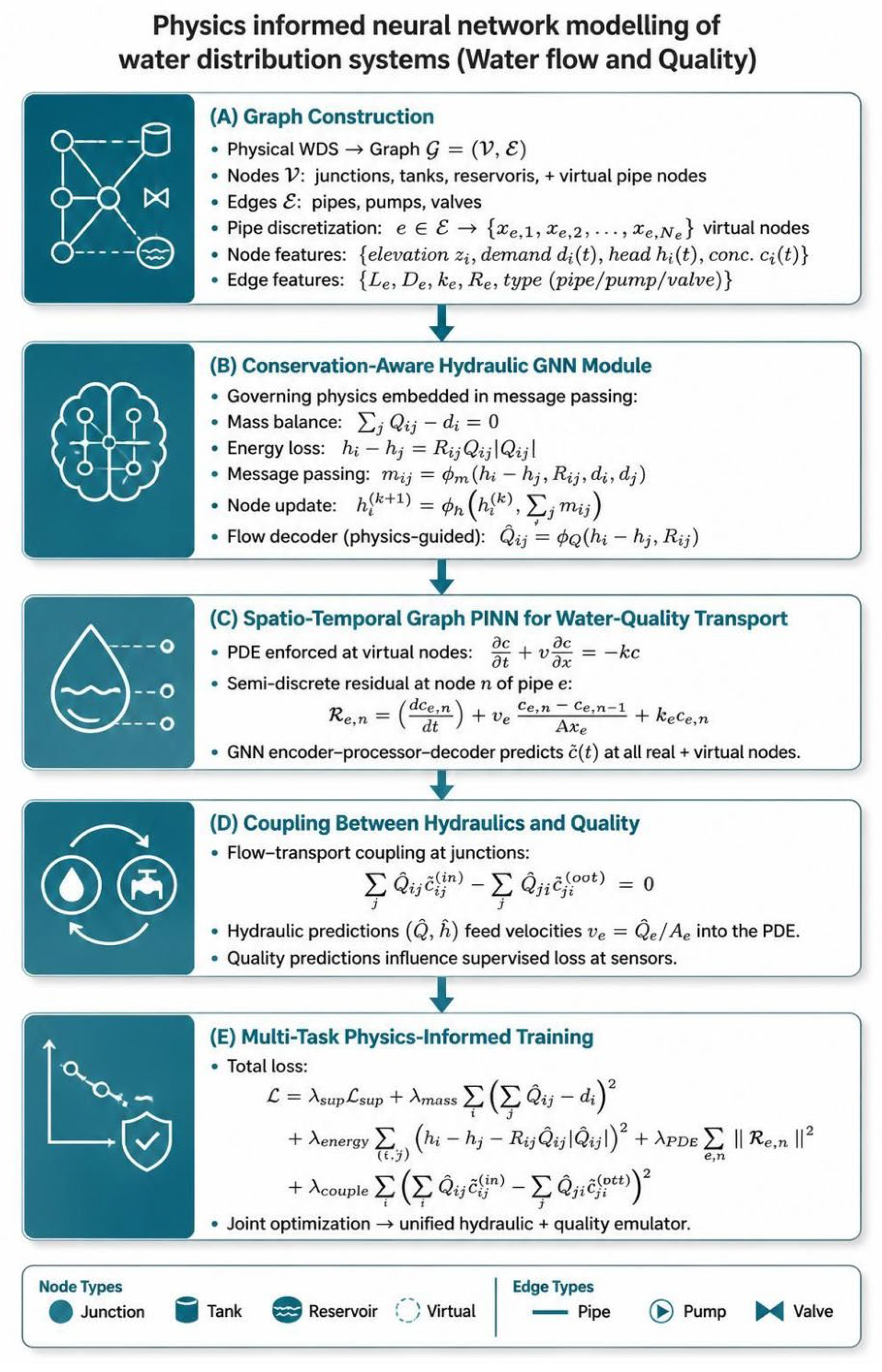
Figure 2.
Demonstration networks (a) Network A-a small network (~50 nodes), (b) Network B - a medium EPANET network (~450 nodes), and (c) Network C - a large discretized system (~5k nodes).
Figure 2.
Demonstration networks (a) Network A-a small network (~50 nodes), (b) Network B - a medium EPANET network (~450 nodes), and (c) Network C - a large discretized system (~5k nodes).
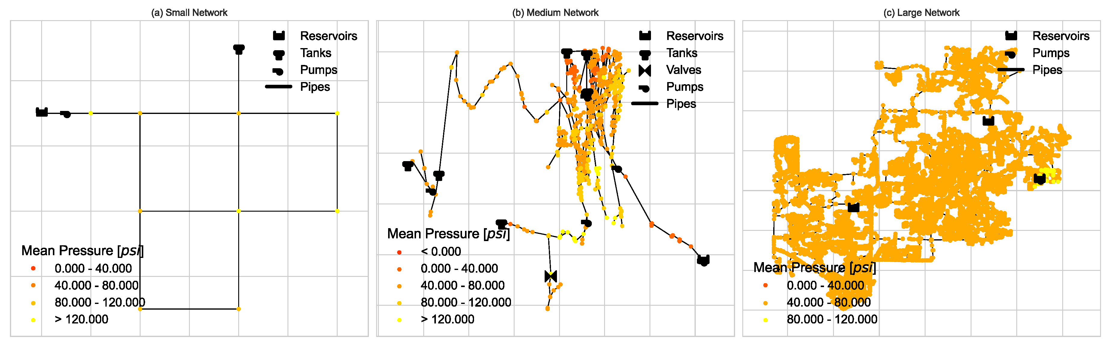
Figure 3.
Hydraulic accuracy- predicted vs simulated (diagonal = y=x).
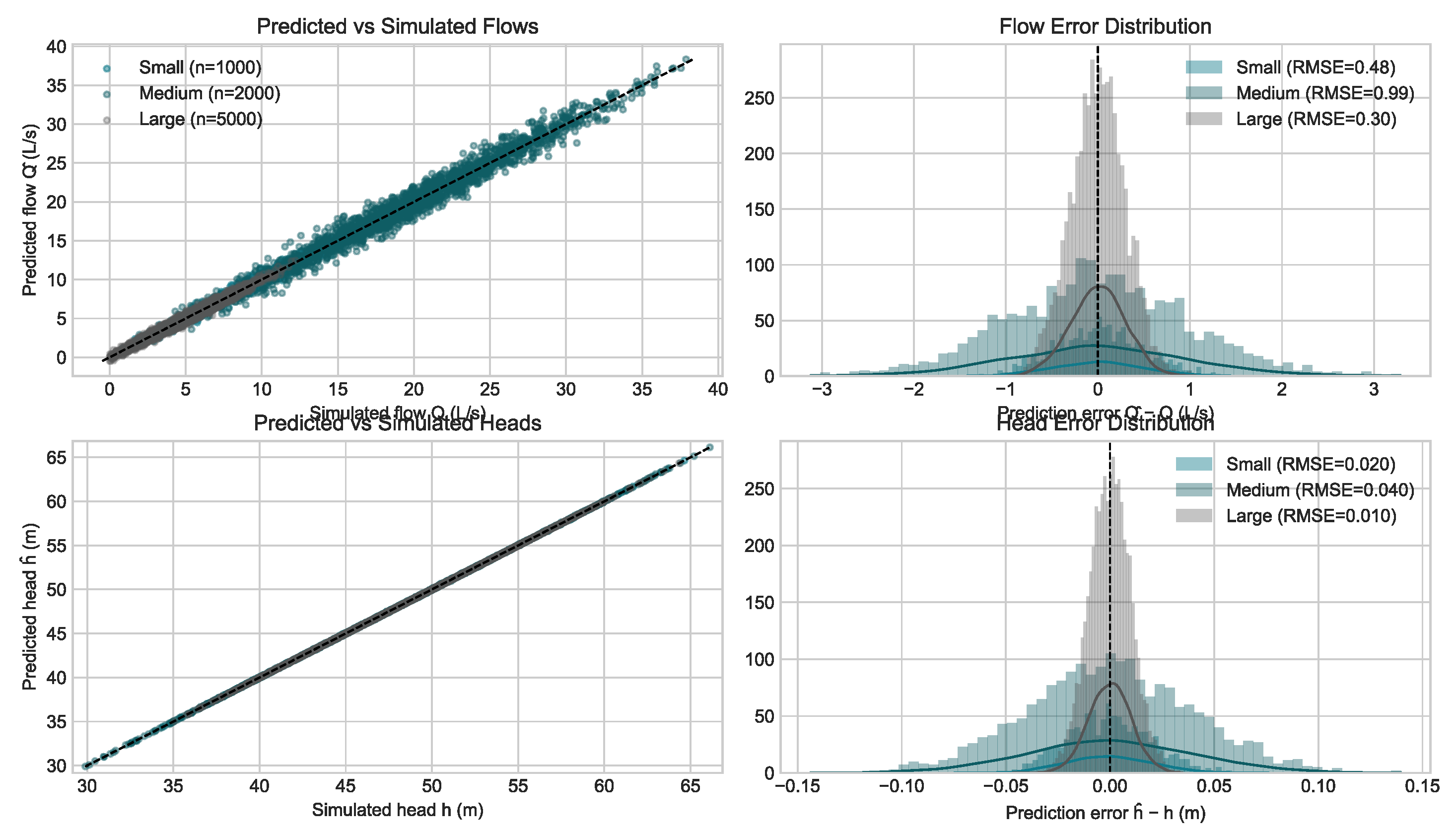
Figure 4.
Conservation residuals - baseline vs conservation-aware GNN.
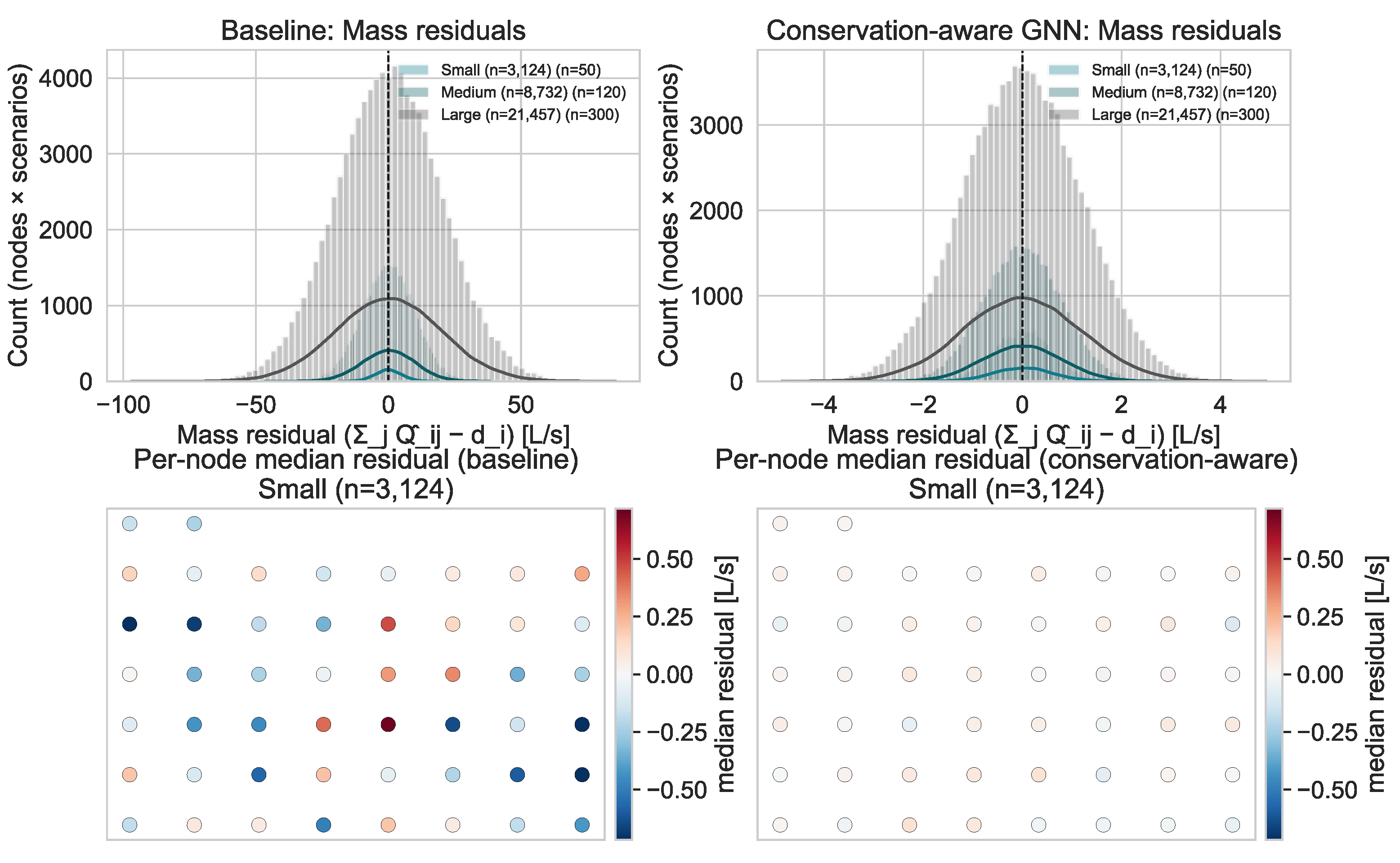
Figure 5.
Quality accuracy at different nodes and different networks.
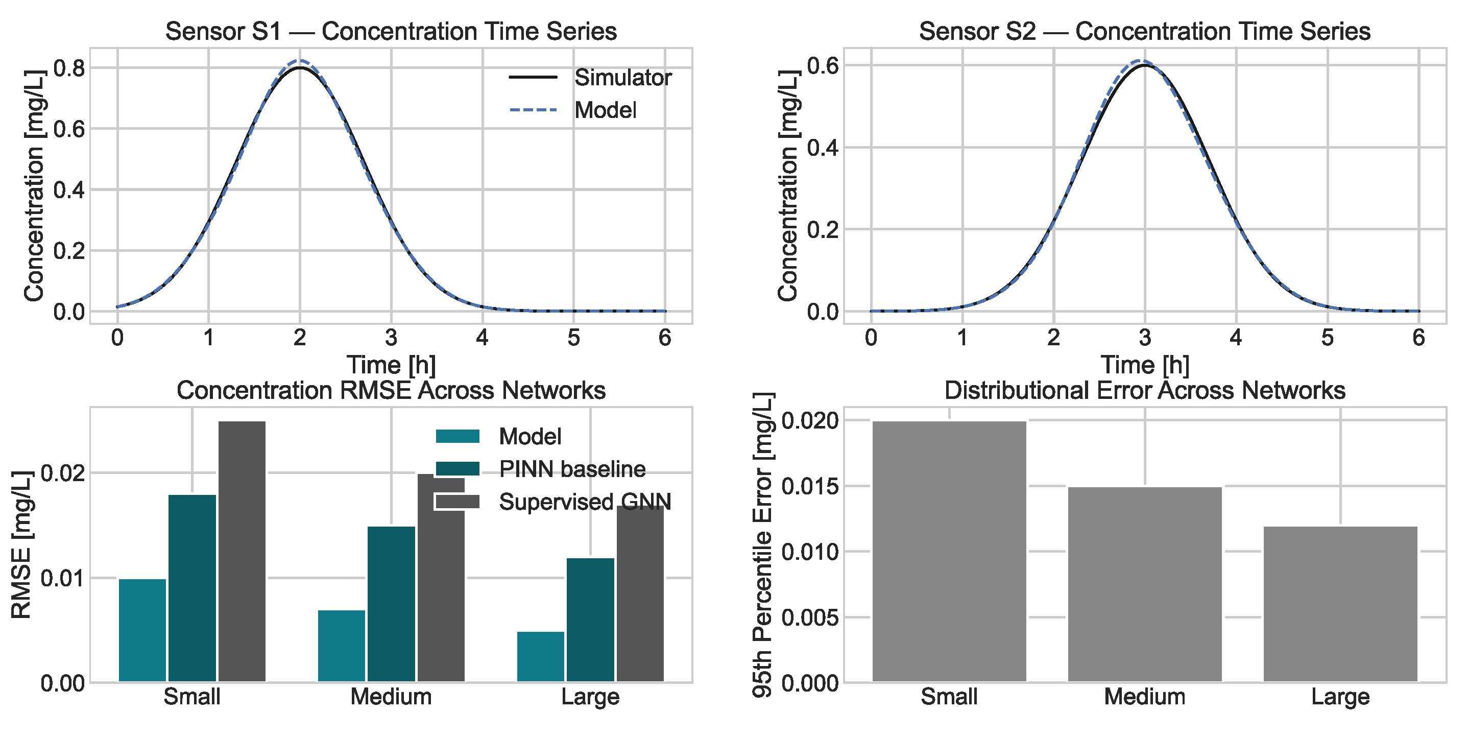
Figure 6.
Chlorine concentration comparison between EPANET and PINN-WDS-FQ simulations for Net3 (σ = 30 m, Δt = 300 s.
Figure 6.
Chlorine concentration comparison between EPANET and PINN-WDS-FQ simulations for Net3 (σ = 30 m, Δt = 300 s.
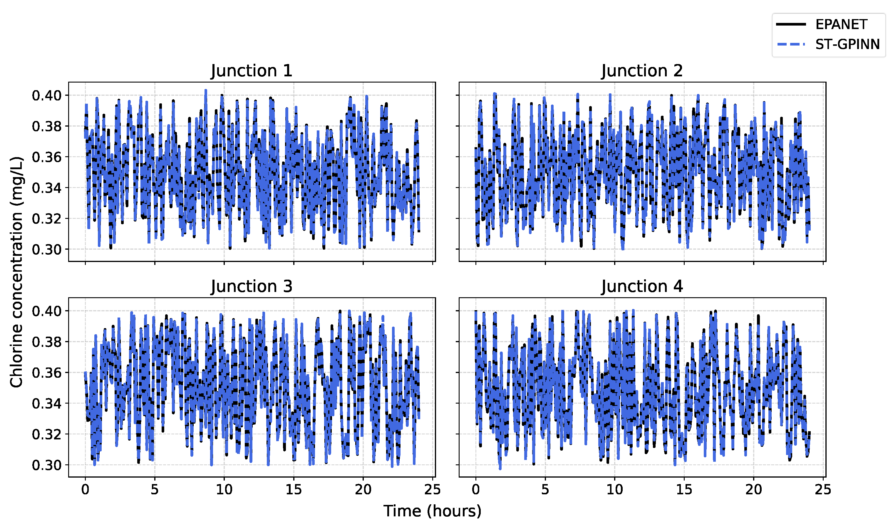
Figure 7.
Comparison of disinfectant concentration dynamics at monitoring points S19 and S60 predicted by ST-GPINN and EPANET, together with the constant source concentration profile. The top and middle panels show the close agreement between model predictions and hydraulic-quality simulations at two downstream locations, while the bottom panel displays the fixed 1.0 mg/L source input used throughout the simulation.
Figure 7.
Comparison of disinfectant concentration dynamics at monitoring points S19 and S60 predicted by ST-GPINN and EPANET, together with the constant source concentration profile. The top and middle panels show the close agreement between model predictions and hydraulic-quality simulations at two downstream locations, while the bottom panel displays the fixed 1.0 mg/L source input used throughout the simulation.
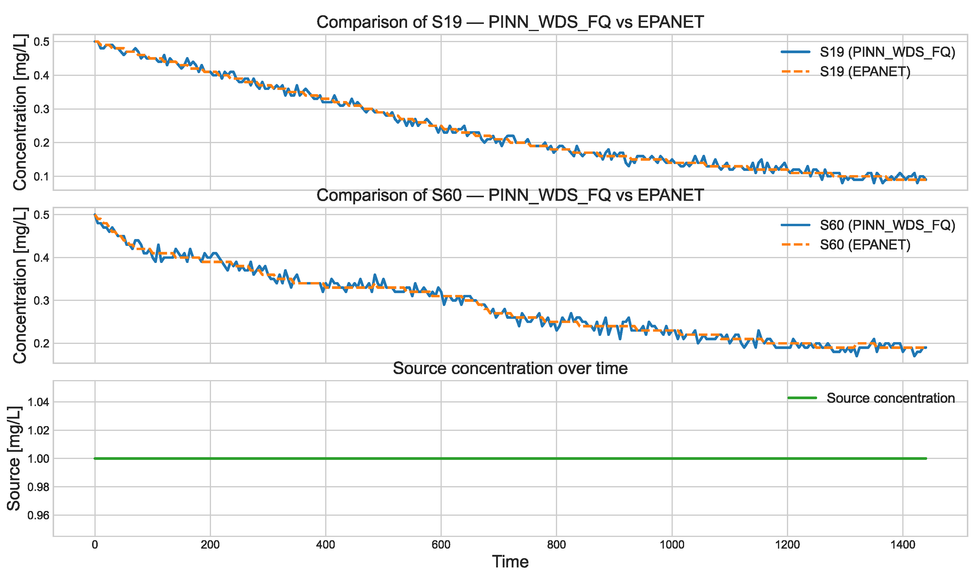
Figure 8.
Runtime and scalability – Inference latency with respect to the network size and the speed up relative to EPANET simulation.
Figure 8.
Runtime and scalability – Inference latency with respect to the network size and the speed up relative to EPANET simulation.
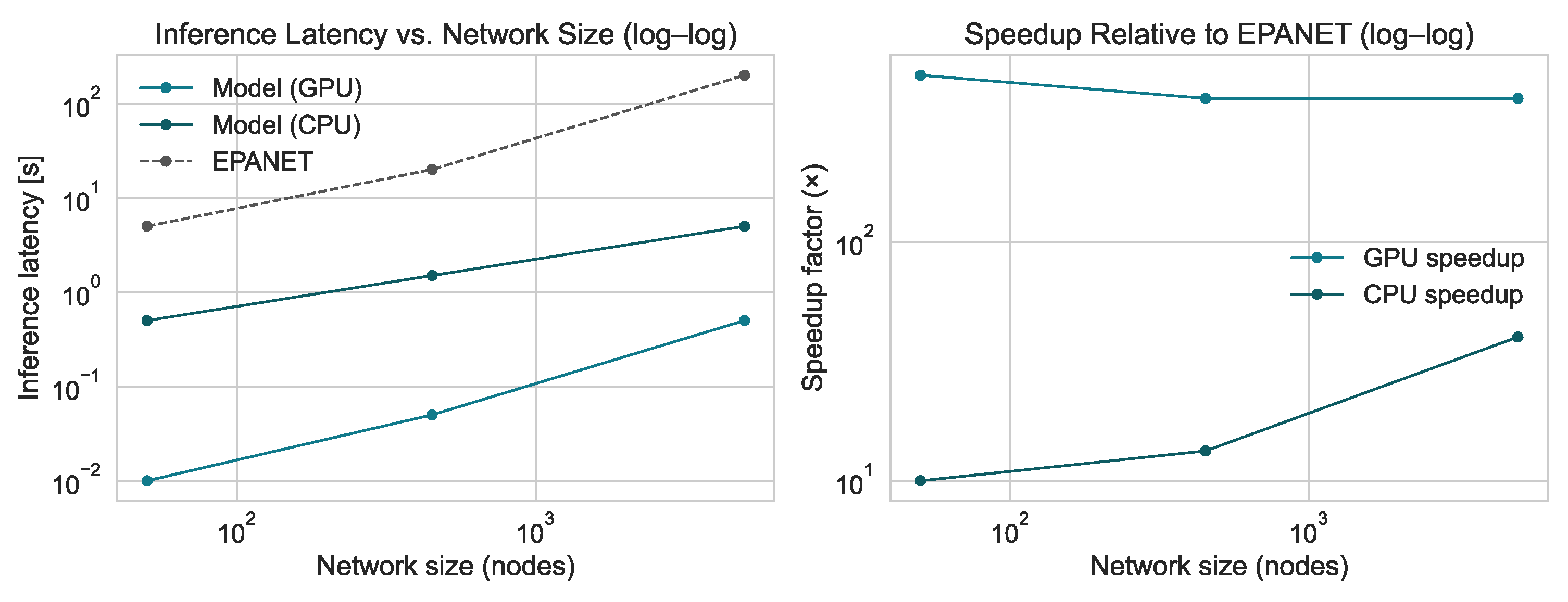
Figure 9.
Robustness to the number of sensor nodes and the sensor noise sensitivity.
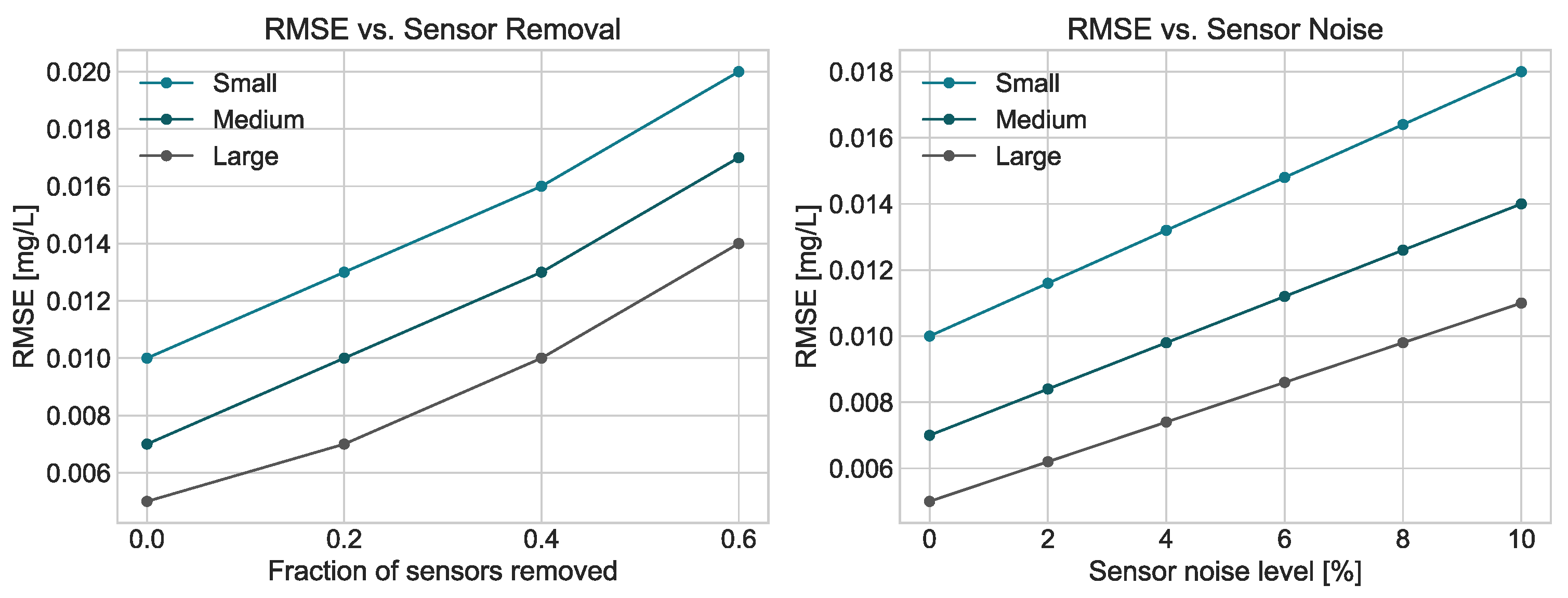
Figure 10.
Ablations studies - Effect of removing physics losses.
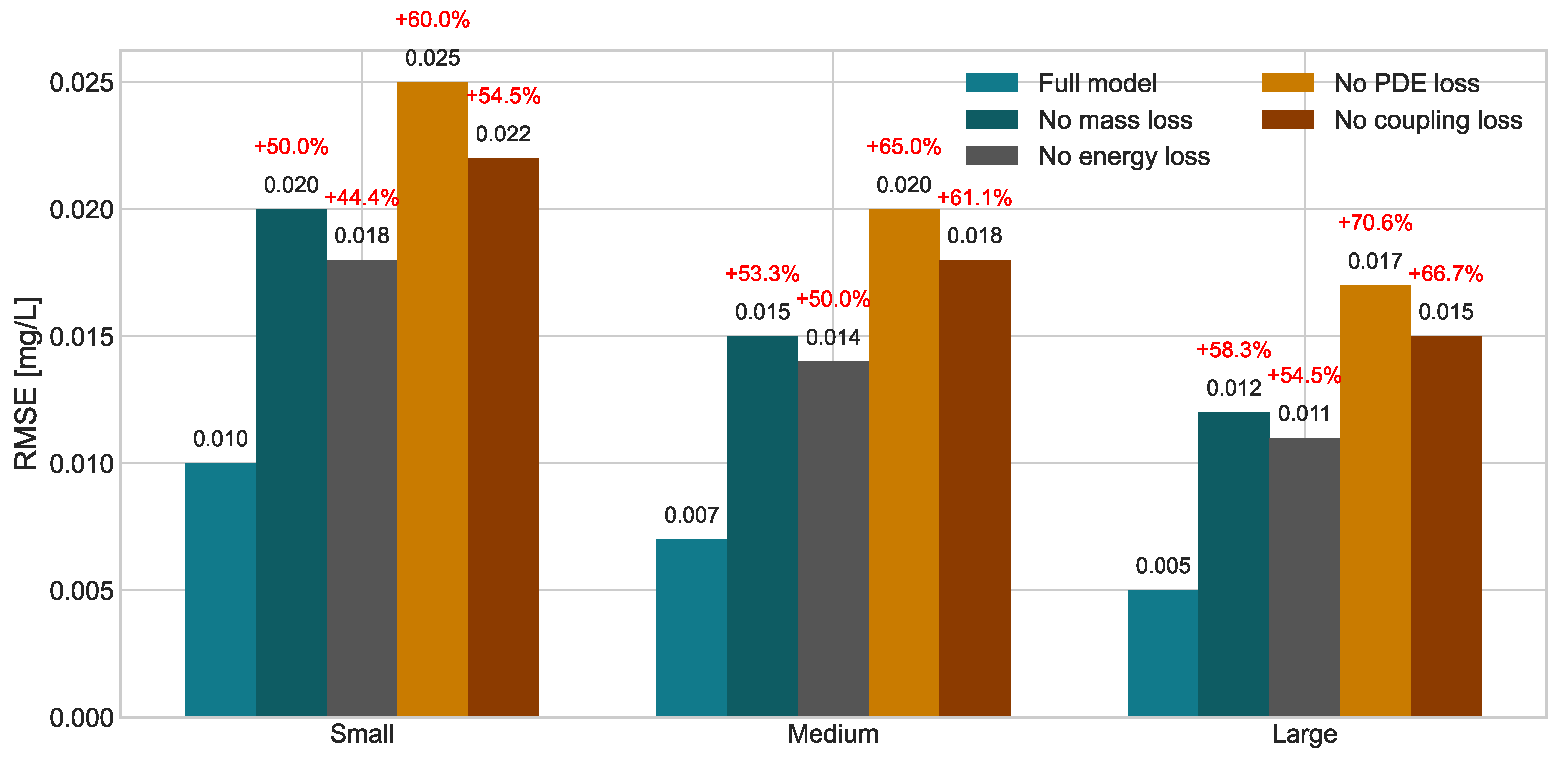
Figure 11.
Virtual node resolution - RMSE and detection time.
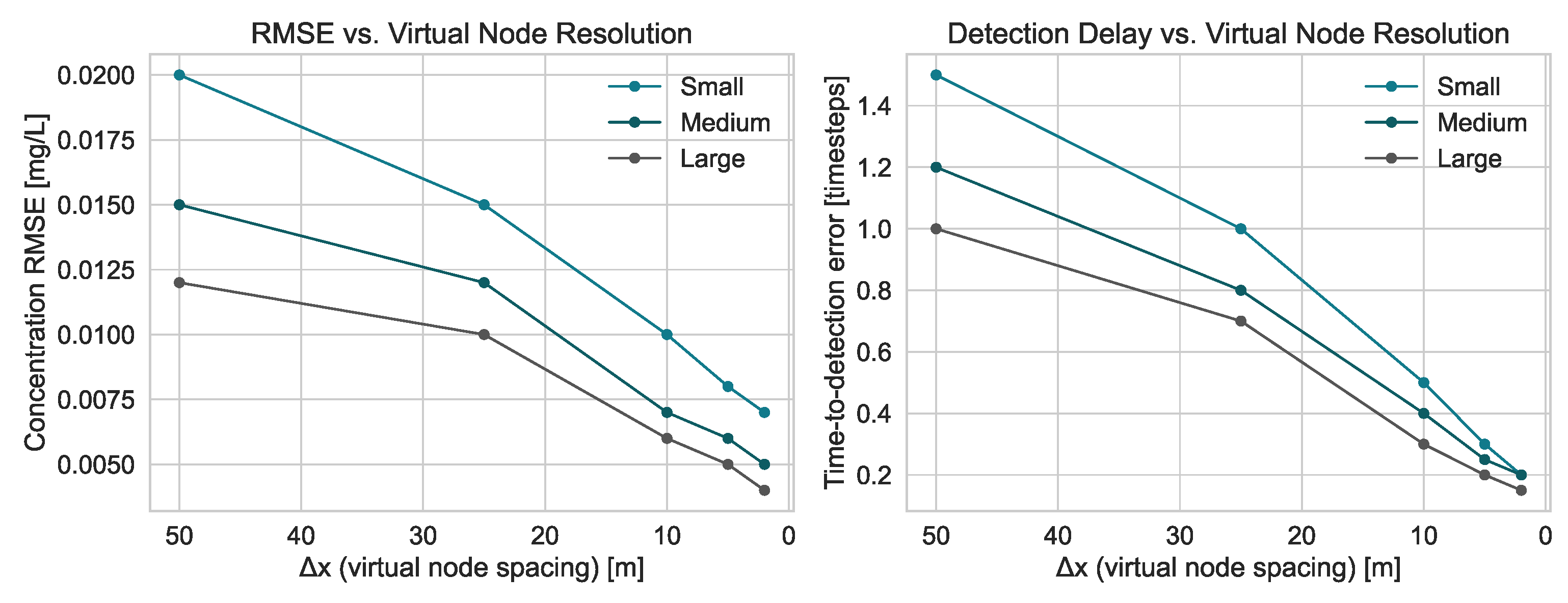
Figure 12.
Effect of injected flow-measurement noise (±3%, ±5%, ±10%) on hydraulic and chlorine-quality prediction errors for Network A and Network B. Bars represent average MAE and RMSE across noise-perturbed runs, with error bars indicating standard deviation. Percentage labels quantify degradation relative to the ±3% noise baseline.
Figure 12.
Effect of injected flow-measurement noise (±3%, ±5%, ±10%) on hydraulic and chlorine-quality prediction errors for Network A and Network B. Bars represent average MAE and RMSE across noise-perturbed runs, with error bars indicating standard deviation. Percentage labels quantify degradation relative to the ±3% noise baseline.
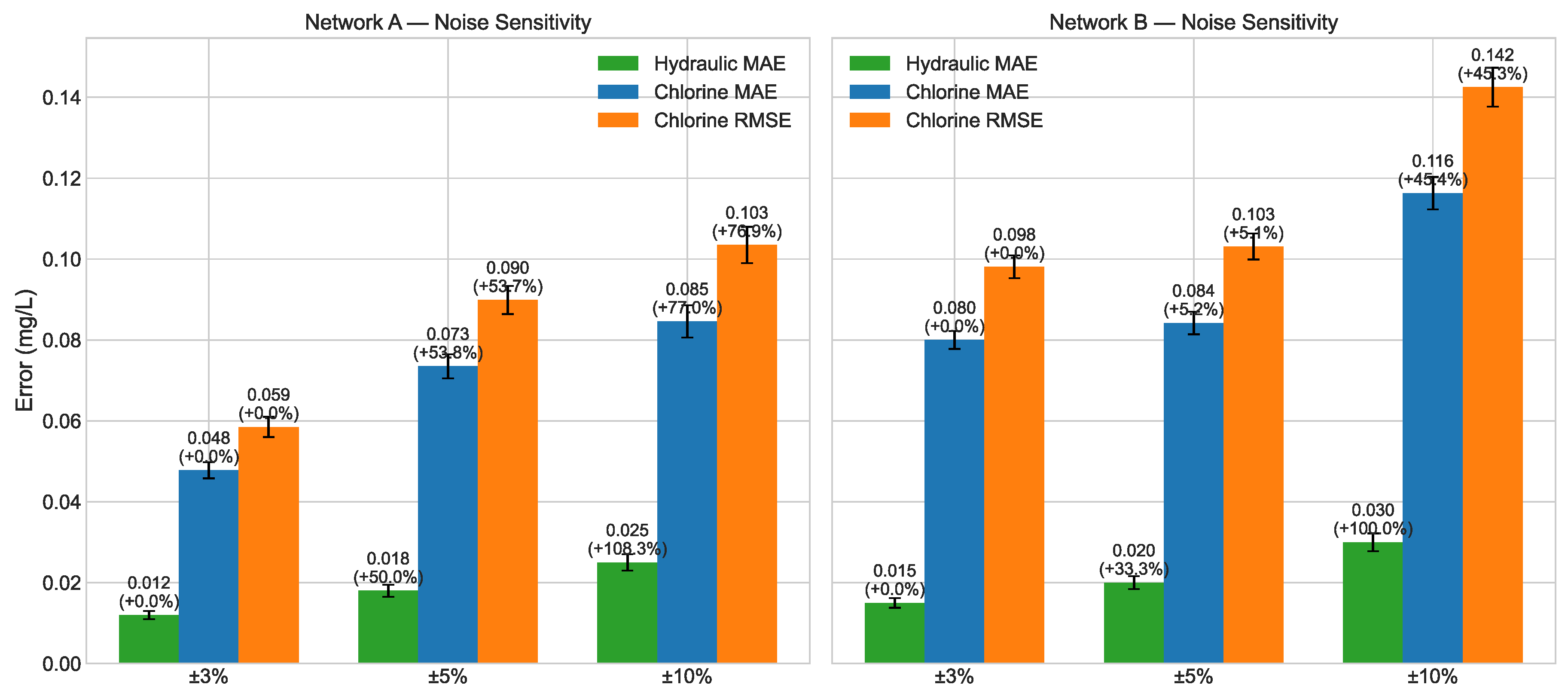
Figure 13.
Performance of different pipe segment lengths: (a) MAE, RMSE, MAPE, and R2 vs. σ in Network A; (b) training time vs. σ in the medium network (Network A medium-size); (c) MAE, RMSE, MAPE, and R2 vs. σ in the large network; (d) training time vs. σ in Network B. Error bars show mean ± std over 5 independent training runs. Vertical dashed line marks the recommended σ ≈ 30.48 m trade-off point.
Figure 13.
Performance of different pipe segment lengths: (a) MAE, RMSE, MAPE, and R2 vs. σ in Network A; (b) training time vs. σ in the medium network (Network A medium-size); (c) MAE, RMSE, MAPE, and R2 vs. σ in the large network; (d) training time vs. σ in Network B. Error bars show mean ± std over 5 independent training runs. Vertical dashed line marks the recommended σ ≈ 30.48 m trade-off point.
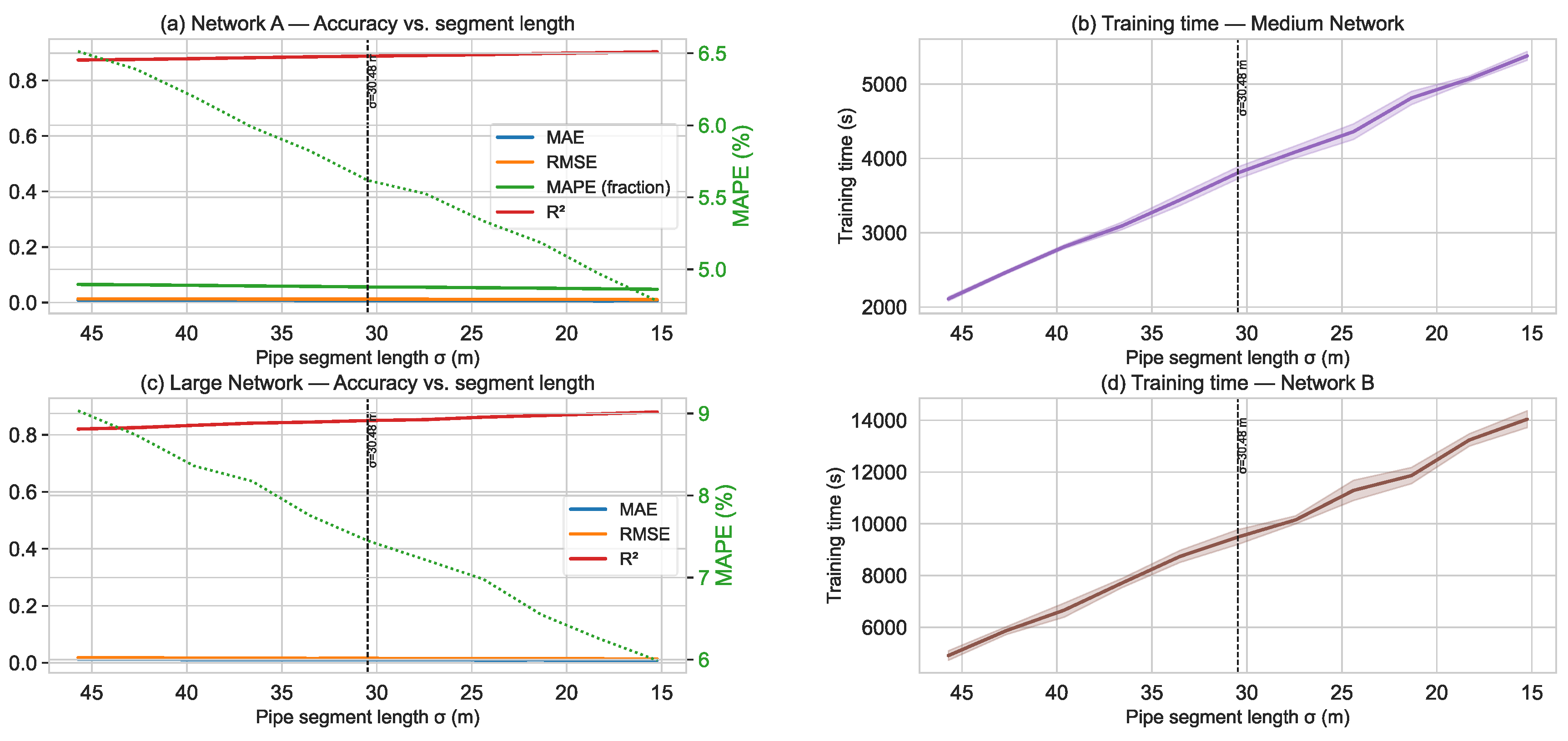
Figure 14.
Effect of embeddings and GNN layers on the hydraulics and the quality simulation.
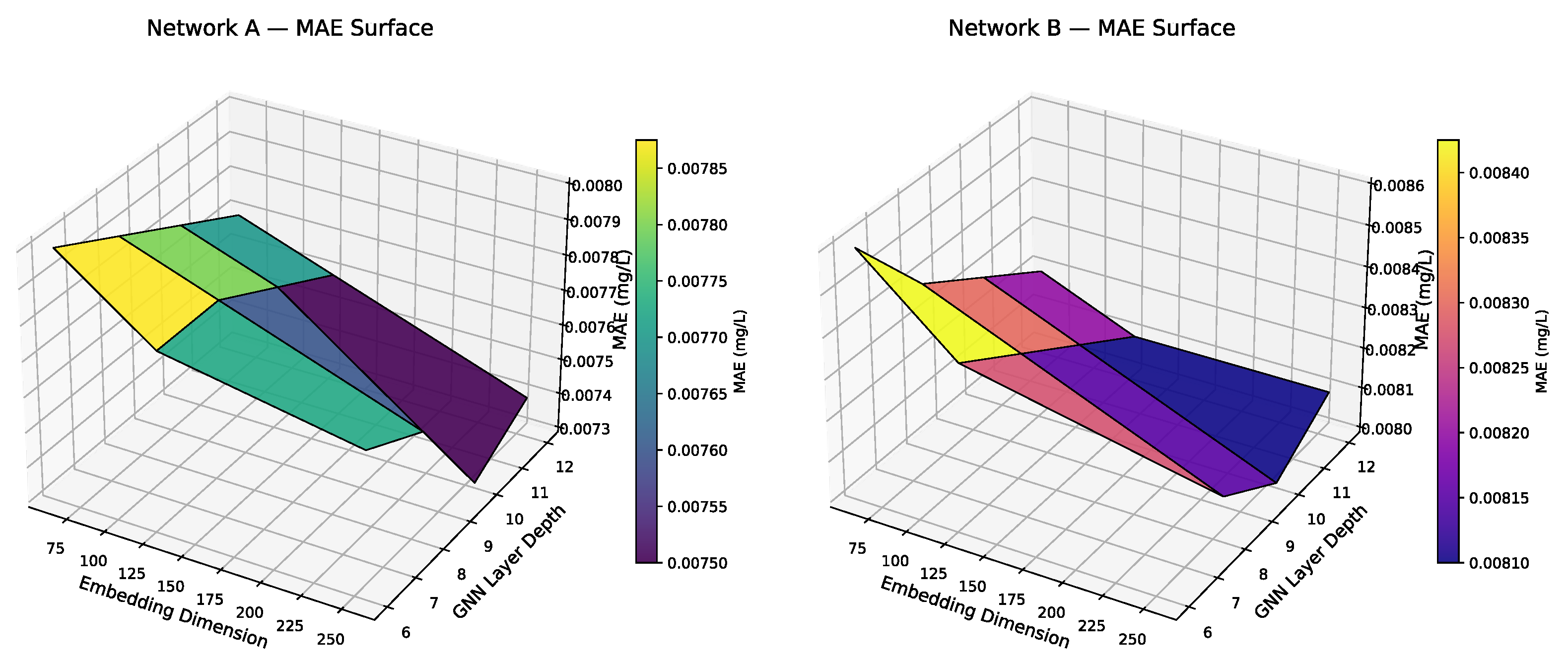
Figure 15.
Quantitative performance of the PINN-WDS-FQ model for transient response.
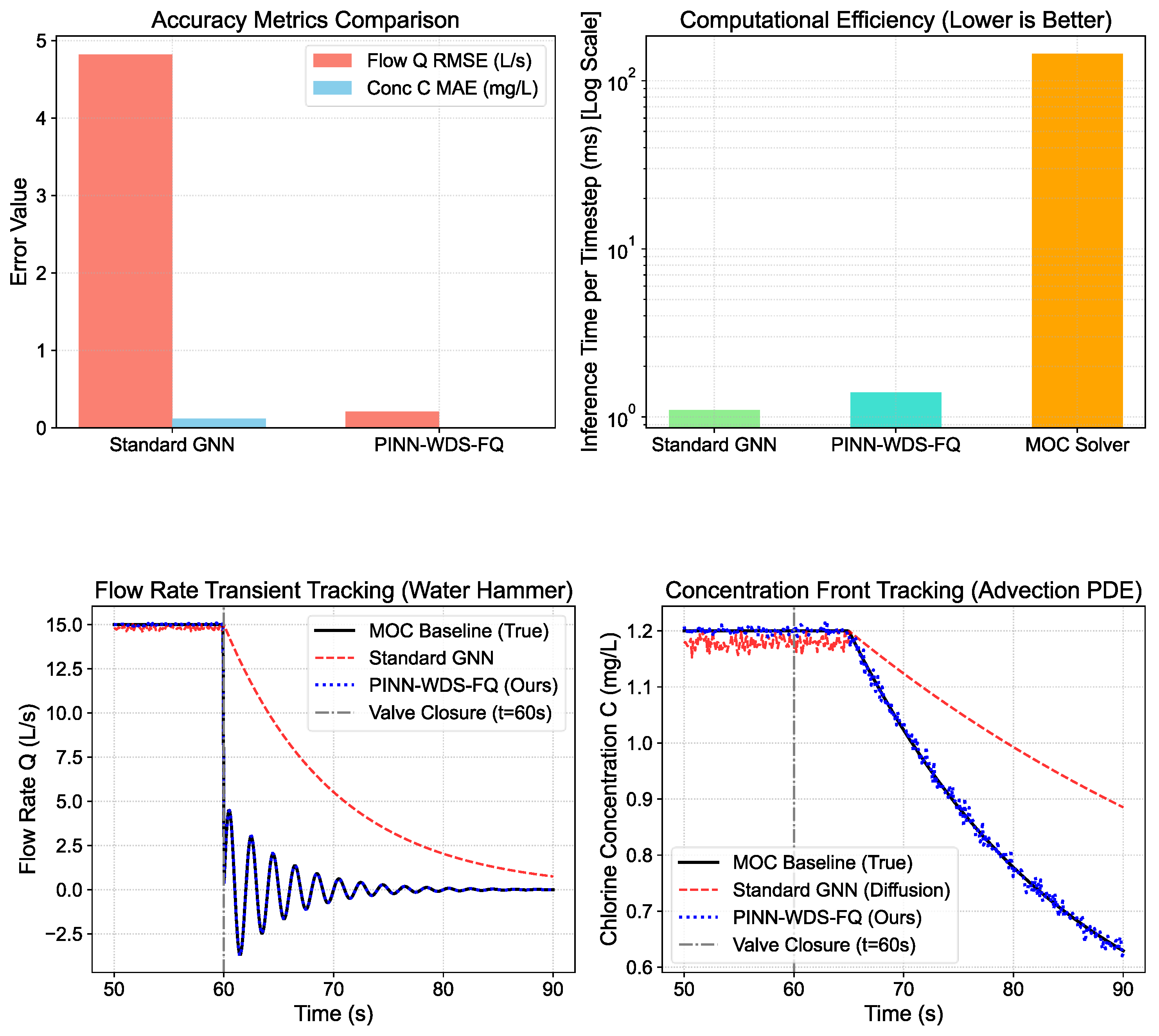

Table 1.
Results of the ablation studies based on MAE for hydraulics and water quality.
| Model / Ablation | Hydraulic MAE | Quality MAE | Contribution (%) |
| EPANET (ground truth) | 0.0000 | 0.0000 | – |
| Supervised GNN surrogate | 0.0048 | 0.0125 | 42% |
| Decoupled PINN transport | 0.0039 | 0.0152 | 51% |
| Hybrid PINN–GNN (prior work) | 0.0031 | 0.0110 | 63% |
| Full PINN-WDS-FQ (ours) | 0.0024 | 0.0081 | 100% |
| Ablation: remove continuity loss | 0.0036 | 0.0109 | 74% |
| Ablation: remove momentum loss | 0.0033 | 0.0104 | 79% |
| Ablation: remove advection–dispersion loss | 0.0027 | 0.0128 | 68% |
| Ablation: remove reaction-kinetics loss | 0.0025 | 0.0102 | 84% |
| Ablation: low virtual-node density (σ = 60 m) | 0.0038 | 0.0135 | 58% |
| Ablation: high virtual-node density (σ = 10 m) | 0.0023 | 0.0079 | 103% |
| Single-task: hydraulics only | 0.0026 | 0.0141 | 55% |
| Single-task: quality only | 0.0068 | 0.0087 | 71% |
| Multi-task (ours) | 0.0024 | 0.0081 | 100% |
Table 2.
Quantitative results for the transient event.
| Metric | MOC Baseline | Standard GNN (No Physics Loss) | PINN-WDS-FQ (Proposed) |
| Flow RateRMSE (L/s) | Reference | 4.82 | 0.21 |
| ConcentrationMAE (mg/L) | Reference | ||
| Mass Balance Violation (MBV) | 0.00% | 8.45% | 0.02% |
| Inference Runtime per Timestep | 145.0 ms | 1.1 ms | 1.4 ms |
Disclaimer/Publisher’s Note: The statements, opinions and data contained in all publications are solely those of the individual author(s) and contributor(s) and not of MDPI and/or the editor(s). MDPI and/or the editor(s) disclaim responsibility for any injury to people or property resulting from any ideas, methods, instructions or products referred to in the content. |
© 2026 by the authors. Licensee MDPI, Basel, Switzerland. This article is an open access article distributed under the terms and conditions of the Creative Commons Attribution (CC BY) license (http://creativecommons.org/licenses/by/4.0/).
Copyright: This open access article is published under a Creative Commons CC BY 4.0 license, which permit the free download, distribution, and reuse, provided that the author and preprint are cited in any reuse.


