
Submitted:
13 August 2026
Posted:
14 August 2026
You are already at the latest version
Abstract
Urban carbon-emission inventories are accounting representations shaped by measurement boundaries, temporal resolution, and analytical scale. This study treats symmetry as a scale-specific reference condition and examines Chinese urban emissions using CEADs annual city accounts for 2001–2019, Carbon Monitor Cities daily estimates for 2019–2021, and harmonized administrative geometries. Distributional, temporal, and local spatial asymmetries are analyzed, with regional Theil decomposition used to characterize inequality composition and cross-inventory concordance used as a robustness assessment. Emissions remained highly concentrated, while long-term inequality trends were sensitive to city coverage. Within-region differences accounted for approximately 96% of standard Theil T inequality. Weekday–weekend asymmetry was small (0.0098), whereas seasonal amplitudes were larger (0.0802–0.1164), and 91.3% of cities shared the same highest-emission season in at least two of three years. Annual global Moran’s I estimates were not significant after false-discovery-rate correction, although recurrent upper-tail imbalance and persistent local states remained evident. The 2019 cross-inventory comparison showed strong concordance in city rankings but more moderate agreement in local spatial classifications. These findings show that apparent urban carbon-emission symmetry depends jointly on analytical scale and accounting construction, highlighting the need to evaluate comparability across alternative measurement bases.
Keywords:
scale-dependent asymmetry
; urban carbon accounting
; carbon-emission inventories
; multiscale analysis
; cross-inventory concordance
1. Introduction
City-level carbon-emission inventories are not simple repositories of physical emission estimates. They are accounting representations shaped by explicit choices about the reporting entity, geographical boundary, sectoral coverage, activity data, emission factors, spatial allocation, and temporal aggregation of emission-generating activities [1,2,3]. From a carbon-accounting perspective, these choices define the measurement basis used to recognize, aggregate, and compare emissions. Consequently, inventories describing broadly the same urban emission system may still produce different totals, rankings, trends, and spatial classifications. This is consistent with the wider carbon-accounting literature, which emphasizes that carbon information is shaped by competing measurement frames and trade-offs among accuracy, consistency, comparability, and uncertainty [4,5,6]. At the city level, these accounting choices affect not only reported emission magnitudes but also which jurisdictions emerge as major emitters, which mitigation priorities become salient, and whether changes remain comparable across time and space. City-level accounts therefore provide an operational basis for differentiated mitigation and monitoring that cannot be recovered from national or provincial aggregates alone [7,8,9,10].
From the perspective of symmetry, however, an urban emission system cannot be characterized adequately by a single aggregate total or average. Symmetry is treated in this study as a scale-specific reference condition rather than as an intrinsic property that must hold uniformly across the system. Distributional symmetry would imply equal emission shares across cities; weekday–weekend symmetry would imply comparable emissions between the two recurring parts of the week; seasonal symmetry would imply limited deviations among seasonal emission profiles; and local spatial-tail symmetry would imply comparable neighbourhood organization of the upper and lower emission tails. These reference conditions need not hold simultaneously. A system may appear approximately symmetric at one scale while remaining strongly asymmetric at another. Distributional inequality is therefore treated as one observable form of departure from an equal-share reference state, rather than as a synonym for asymmetry in all dimensions. The equal-share condition is used solely as a mathematical reference state for distributional symmetry; it does not imply that equal total emissions across cities of different population or economic size would constitute a normative, equitable, or policy-optimal allocation. Related emissions research has similarly used asymmetry to identify departures from homogeneous responses across technologies, operating conditions, and observational scales [11].
From an accounting perspective, the relevant reference condition depends on the analytical attribute under examination: concentration, temporal comparability, or spatial organization. A single notion of symmetry should therefore not be transferred mechanically across these measurement dimensions.
This scale dependence has direct implications for the decision usefulness of urban carbon accounts. Carbon-accounting research has long emphasized that measurement is useful only when reported information can be interpreted with sufficient transparency, consistency, and awareness of uncertainty [5,12]. For urban inventories, decision usefulness therefore depends not only on the reported aggregate quantity but also on whether the underlying measurement basis is sufficiently transparent and whether the structures derived from that quantity remain comparable across reporting systems. Inventory-based accounts, satellite-assisted downscaling products, and near-real-time activity-based datasets may differ in sectoral boundaries, spatial allocation rules, temporal frequencies, and estimation procedures. Such differences are not merely technical preprocessing details; they are accounting-design choices that can affect classification and comparison. Consequently, cross-inventory agreement should be evaluated empirically rather than assumed [13]. This issue becomes especially important when emission information is used to rank cities, identify high-emission jurisdictions, or classify local spatial patterns, because similar aggregate totals need not produce equivalent city-level information [14,15,16].
At the distributional scale, carbon inequality studies commonly employ the Gini coefficient, the standard Theil T index, top-emitter shares, and related decomposition methods. Existing evidence has documented unequal household carbon footprints, disparities in residential-building emissions, and substantial differences in energy-related emissions across Chinese cities [17,18,19,20]. These studies demonstrate that emission burdens are unevenly distributed, but the estimated level and direction of inequality depend on the analytical unit and accounting basis. Per-capita emissions, household footprints, residential emissions, carbon intensity, and total territorial city emissions need not generate the same rankings or decomposition patterns [20,21,22]. The present analysis therefore concerns the concentration of total city-level fossil-fuel emissions. It does not interpret the resulting indices as measures of household welfare, consumption inequality, or per-capita equity.
Regional decomposition provides a related but distinct compositional perspective. The standard Theil T index can partition observed inequality into differences between broad regions and differences among cities within the same region. A similar national inequality level may therefore correspond to fundamentally different spatial compositions. If between-region differences dominate, broad regional categories may capture a substantial part of the observed structure. If within-region differences dominate, regional averages may conceal important city-level heterogeneity. The decomposition is interpreted here as a compositional partition of observed inequality, rather than as evidence that regional location causes emission differences or as an allocation of legal responsibility [18,20].
Temporal resolution introduces a further source of scale dependence. Conventional city inventories are generally annual and are therefore appropriate for identifying long-term structural changes, but they cannot directly reveal weekday–weekend cycles, seasonal contrasts, or short-term disturbances. Carbon Monitor and Carbon Monitor Cities provide daily estimates that make these recurring temporal structures observable [15,16,23]. Recent studies have used such data to examine daily peaks, seasonal patterns, and responses to exceptional events [24]. Nevertheless, short-cycle variation has usually been examined separately from long-term intercity inequality. For near-real-time carbon accounting, this separation matters because a short-term observation should be evaluated relative to an appropriate temporal baseline. A directionally consistent weekday–weekend contrast may be substantively small, whereas a seasonal contrast may be larger and more persistent. Direction, magnitude, and cross-year recurrence must therefore be distinguished.
Spatial asymmetry poses a similar interpretive problem. Global Moran’s I summarizes average neighbourhood dependence across the complete sample, whereas local tail organization concerns whether high-emission and low-emission cities form same-tail connections with comparable prevalence. Local-state persistence addresses yet another question: whether high–high and low–low configurations remain stable across consecutive years. From a broader graph-theoretic perspective, network organization can be characterized through distinct structural properties such as edge orientation, connectivity, and path-based organization [25,26,27]. These properties are not interchangeable, reinforcing the need to distinguish global dependence, local configuration, and persistence when characterizing spatial structure. Related spatio-temporal graph modelling has also shown the value of explicitly representing dynamic dependence structures in non-stationary systems [28]. A weak or statistically unstable global statistic does not imply that the upper and lower tails are organized symmetrically, just as a difference in tail prevalence does not imply that one local state is more persistent than the other. Previous studies have reported spatial heterogeneity and local clustering in Chinese urban emissions, but the relationship varies across locations, city types, and analytical scales [29,30,31,32,33]. The present study therefore separates global dependence, tail-specific connection prevalence, and local-state persistence without presuming causal spatial spillovers.
A final challenge concerns whether the derived structures are reproducible across independently constructed emission inventories. Cross-inventory comparison is often treated as a technical validation exercise focused on aggregate quantities. However, agreement in total emissions does not necessarily imply agreement in city rankings, top-emitter sets, spatial lags, or local-state classifications. Conversely, inventories may preserve similar relative city positions while differing in absolute quantities because of alternative accounting boundaries and allocation procedures. Cross-inventory concordance is therefore interpreted here as evidence of reporting robustness, not as proof that either inventory provides an error-free ground truth. This distinction connects the statistical analysis of asymmetry with the accounting concerns of measurement comparability, boundary sensitivity, and transparent reporting.
Against this background, this study develops an accounting-aware, scale-dependent framework for examining asymmetry in Chinese urban carbon emissions. Four analytical components are retained. Distributional asymmetry describes the concentration of emissions across cities. Regional Theil decomposition identifies the within-region and between-region composition of that inequality. Temporal asymmetry is represented by weekday–weekend and seasonal contrasts. Local spatial asymmetry is represented by upper–lower tail organization and the persistence of high–high and low–low states. Cross-inventory concordance is evaluated separately as an external robustness layer rather than as a fifth asymmetry dimension.
Empirically, the framework integrates a harmonized CEADs longitudinal city panel for 2001–2019, Carbon Monitor Cities daily estimates for 2019–2021, and harmonized administrative geometries. The analysis combines distributional indices, regional Theil decomposition, temporal contrast measures, and global and local spatial statistics. A strictly matched 2019 comparison evaluates whether city rankings and local spatial structures are reproduced across the two inventories. Multiple trend estimators, resampling procedures, false-discovery-rate correction, influential-city tests, and sample-sensitivity analyses are used to distinguish persistent findings from conclusions that depend on a particular indicator, sample, or inventory.
This study addresses the following research questions:
- 1.
- How does Chinese urban carbon-emission asymmetry vary across distributional, temporal, and spatial scales, and which findings remain stable across alternative samples and indicators?
- 2.
- What distinct structures are revealed by regional inequality decomposition, short-cycle and seasonal temporal contrasts, and persistent local spatial-tail configurations?
- 3.
- To what extent are city rankings and local spatial structures reproduced across independently constructed emission inventories with different accounting and measurement procedures?
This study makes three main contributions. First, it conceptualizes urban carbon-emission symmetry as a scale-specific reference condition rather than as a uniform property of the emission system. This framework explains how weak asymmetry at one scale can coexist with pronounced and persistent asymmetry at another, while avoiding the assumption that distributional inequality, temporal contrast, and spatial organization represent the same phenomenon.
Second, the study develops an accounting-aware multiscale analytical design that treats reporting boundary, measurement basis, temporal resolution, and sample construction as substantive determinants of the resulting evidence rather than as neutral preprocessing choices. Annual inventories, daily estimates, regional decompositions, and spatial classifications are assigned distinct analytical roles instead of being pooled as interchangeable measurements. This design links the statistical analysis of asymmetry with the accounting principles of measurement consistency and comparability by explicitly separating inequality levels from inequality trends, contrast direction from contrast magnitude, and global spatial dependence from local tail organization.
Third, the study extends cross-inventory assessment from aggregate reconciliation to structural concordance. By evaluating city rankings, top-emitter overlap, influential-city sensitivity, spatial-lag agreement, and local-state concordance, the analysis examines whether decision-relevant urban emission structures are reproducible across independently constructed emission inventories with different accounting procedures. Concordance in relative structure increases confidence in comparative reporting, whereas disagreement identifies dimensions that remain sensitive to measurement boundaries and inventory construction.
The methodological contribution lies not in proposing new versions of established inequality, temporal, or spatial statistics, but in defining scale-specific symmetry reference states, assigning non-interchangeable inventory products to those states, and evaluating which conclusions remain stable across alternative samples, temporal resolutions, spatial definitions, and independently constructed emission inventories.
Figure 1 summarizes the conceptual structure. The distributional, regional, temporal, and local spatial components are treated as complementary rather than sequential, while the 2019 cross-inventory comparison serves as a separate accounting-robustness layer.
2. Materials and Methods
2.1. Overall Study Design
This study integrates three complementary data components to examine urban carbon-emission asymmetry at multiple temporal and spatial scales. First, the CEADs longitudinal city-level emission accounts are used to characterize long-term distributional inequality and to conduct a separate standard Theil T decomposition in the region-mapped sample. Second, Carbon Monitor Cities daily estimates are used to evaluate weekday–weekend and seasonal asymmetries. Third, GADM administrative geometries are used to construct spatial weights and examine global dependence, local tail clustering, and local-state persistence.
The datasets were not mechanically pooled into a single regression sample. Instead, each source was assigned a specific analytical role according to its accounting boundary, temporal resolution, city coverage, and estimation procedure. Cross-inventory analyses were conducted only for cities and years that could be matched under a common city-identity system. This design avoids treating annual inventories and daily estimates as directly interchangeable measurements. More generally, it follows a basic carbon-accounting requirement: measurements constructed under different reporting entities, boundaries, temporal bases, or allocation procedures should not be treated as directly comparable until their analytical roles and harmonization rules are explicitly disclosed.
2.2. CEADs Longitudinal City-Level Emissions
The long-term analysis is based on city-level fossil-fuel CO2 emission accounts compiled within the China Emission Accounts and Datasets framework [7,8]. The source data cover the period from 1997 to 2019. To improve temporal comparability and reduce the influence of early-year data gaps, the principal analytical window was restricted to 2001–2019.
Two principal longitudinal samples were retained. The full longitudinal sample, denoted by , contains 289 cities and is used mainly to assess sensitivity to expanded city coverage. The strict core sample, denoted by , contains 72 cities with relatively stable longitudinal coverage and serves as the principal sample for annual inequality trends and local-state persistence.
Regional decomposition is evaluated separately on a region-mapped longitudinal sample, denoted by . Depending on annual data availability, this sample contains between 56 and 65 valid cities per year. It is retained separately because valid macro-region assignments are required for every included city.
Only observed city-year emission values were used. Missing emissions were neither imputed nor replaced by zero. The number of cities entering an annual calculation may therefore vary across years. During 2001–2019, the annual valid-city count ranged from 63 to 72 in and from 106 to 263 in . The principal variable is total city-level fossil-fuel CO2 emissions. Results based on total emissions are not interpreted as per-capita emissions, carbon intensity, or consumption-based carbon footprints.
2.3. Carbon Monitor Cities Daily Emissions
Daily urban emissions are obtained from Carbon Monitor Cities, which provides near-real-time estimates for cities worldwide and covers power generation, industry, residential and commercial buildings, ground transport, and aviation [15]. The Chinese data used in this study cover 2019–2021.
The original records are organized by city, date, and sector. For the temporal analysis, the five sectoral components reported by Carbon Monitor Cities were aggregated into city-day total emissions. The resulting daily analytical sample, denoted by D, contains 311 Chinese cities.
The daily data are used to evaluate weekday–weekend differences, seasonal deviation profiles, seasonal amplitude, and cross-year peak-season recurrence. Sectoral aggregation is used only to construct daily city totals; no sector-concentration or fuel-structure conclusions are derived from these aggregated values.
The year 2020 is reported separately because it represents an unusual disturbance period. However, observed changes in 2020 are treated as descriptive heterogeneity rather than being automatically attributed to a single causal mechanism.
2.4. City-Identity Harmonization and Matched Samples
A common city-identity system was constructed before combining information from different sources. Each analytical unit was assigned a unique master_unit_id. Matching was based on the joint identity of province and city, rather than on city names alone.
The harmonization process incorporated exact province–city matches, curated aliases, historical administrative-name changes, and manual review of ambiguous cases. Special attention was paid to cities sharing the same Romanized or English name across different provinces. Automatic acceptance of fuzzy name matches was not permitted.
For the 2019 cross-inventory comparison, the five Carbon Monitor Cities sectoral estimates were first aggregated within each city and date and then summed over the complete calendar year. Only city-year records containing all five sectors and 365 distinct dates were retained. The resulting annual Carbon Monitor Cities values are expressed in and were matched to CEADs 2019 estimates under the common city-identity system.
For cross-inventory comparison, CEADs and Carbon Monitor Cities were aligned for the common year 2019. The non-spatial matched sample, denoted by C, contains 158 cities with valid emission observations in both sources. These cities are used to evaluate rank correlations, top-emitter overlap, and sensitivity to influential observations.
The spatially eligible subset, denoted by , contains 153 of the 158 matched cities. The remaining five cities were excluded only from the spatial comparison because a unique and compatible geometry could not be established. They remain part of the non-spatial cross-inventory analysis.
2.5. Spatial Geometry and Boundary Harmonization
Prefecture-level geometries were obtained from GADM version 4.1 at the second administrative level. The source geometries use the WGS84 geographic coordinate system. For distance-based spatial weights, the geometries were projected to a China Albers equal-area coordinate system before representative points and pairwise distances were calculated.
The principal spatial analysis uses polygon representative points because they are guaranteed to fall within the corresponding administrative geometry. Polygon centroids are retained only for sensitivity checks. Euclidean distances were not calculated directly from longitude and latitude.
A time-invariant harmonized boundary framework was used for the 2001–2019 longitudinal analysis. This choice ensures that changes in spatial weights do not mechanically reflect changes in administrative boundaries. The modern GADM geometry should therefore be understood as a common analytical frame rather than as an exact reconstruction of the administrative boundary in every historical year. Administrative changes are not interpreted as emission changes.
2.6. Analytical Sample Architecture
Table 1 summarizes the analytical samples used in the study. Separate samples are retained because the underlying datasets differ in temporal frequency, coverage, and analytical purpose.
2.7. Data Quality Control and Reproducibility
Before formal inference, data versions, city identities, and sample-eligibility rules were fixed. Quality control included checks for duplicate city identities, one-to-many and many-to-one matches, missing province information, invalid dates, duplicate geometries, inconsistent administrative mappings, and accounting-level ambiguity. Missing emissions were not imputed, and non-significant years were not selectively removed.
From an accounting perspective, these procedures also serve as measurement controls intended to preserve reporting-entity consistency and to reduce the risk that changes in sample coverage or administrative identity are misinterpreted as changes in the underlying emission structure.
Versioned analytical scripts, file checksums, and fixed random seeds were retained by the authors. Bootstrap, permutation, and sensitivity analyses were conducted using prespecified procedures. Weak and non-significant findings, including weak global spatial dependence and the small weekday–weekend contrast, were reported alongside the stronger results.
ChatGPT (OpenAI) and Claude (Anthropic) were used only as auxiliary tools for language refinement and non-substantive technical checking during manuscript preparation. They were not used to determine the research questions, methodological design, statistical results, data interpretation, or scientific conclusions. All analytical scripts, outputs, and manuscript revisions were reviewed by the authors.
2.8. Overview and Notation
The analytical framework evaluates urban carbon-emission asymmetry across distributional, temporal, and local spatial dimensions, while regional Theil decomposition characterizes the composition of inequality. Let denote the observed total CO2 emissions of city i in year t, and let denote the number of cities with valid observations in a given analytical sample and year. The corresponding observed sample total is
The meaning of and is therefore specific to the analytical sample used in each module. Only observed emissions are included in each annual calculation. Missing city-year values are not imputed and are not replaced by zero. Consequently, may vary across years.
For the daily analysis, denotes the total daily emissions of city i on calendar day d. For seasonal analysis, denotes the mean daily emissions of city i in year y and season s. Spatial analyses use log-transformed emissions,
as the principal variable to reduce the influence of a small number of extremely high-emission cities. Raw emissions and annual emission ranks are retained as sensitivity variables.
The term asymmetry is evaluated relative to module-specific reference states. Distributional symmetry corresponds to equal emission shares across cities, for which . This reference state is mathematical rather than normative and is not interpreted as an equitable allocation of total emissions across differently sized cities. Weekday–weekend symmetry corresponds to , seasonal symmetry corresponds to and , and upper–lower tail symmetry corresponds to . Local-state persistence is assessed by comparing and with each other and with randomized baselines. Regional decomposition is interpreted as compositional imbalance between within-region and between-region contributions rather than as a formal symmetry test. Cross-inventory concordance is treated as an external robustness layer rather than as a fifth asymmetry dimension.
2.9. Long-Term Distributional Asymmetry
2.9.1. Gini Coefficient
The Gini coefficient is used to quantify the overall dispersion of emissions across cities. For year t, it is calculated as
where
A larger indicates a more unequal distribution of city-level emissions. The coefficient is interpreted as a measure of distributional concentration rather than as a measure of per-capita inequality or welfare inequality.
2.9.2. Standard Theil T Index
Following the information-theoretic formulation of inequality [34], the Theil T index is calculated as
The standard Theil T index equals zero under an equal distribution and increases as a larger proportion of total emissions becomes concentrated in fewer cities. Unlike the Gini coefficient, it is additively decomposable and can therefore be separated into within-region and between-region components.
Long-term standard Theil T trends are estimated separately for and . Regional decomposition is evaluated on . Because annual city coverage differs across these samples, the region-mapped total Theil T series is sample-specific and is not treated as an exact decomposition of the series.
2.9.3. Top-Emitter Shares
To provide a direct interpretation of upper-tail concentration, the share of total emissions produced by the highest-emitting proportion p of cities is defined as
where denotes the set of cities in the top p proportion of the annual emission distribution. The top-10% and top-20% shares, the coefficient of variation, and the ratio between the 90th and 10th percentiles are retained as additional descriptive measures.
2.10. Trend Estimation and Robustness Inference
For each annual inequality indicator , a descriptive linear trend is estimated as
Because annual inequality measures may exhibit serial correlation and heteroskedasticity, statistical inference for uses Newey–West heteroskedasticity- and autocorrelation-consistent standard errors [35]. The canonical implementation uses a Bartlett kernel, a lag length of for the 19 annual observations, an intercept, a finite-sample covariance correction, and two-sided t-based inference with degrees of freedom.
Given the short annual series, this specification is treated as a prespecified inferential convention rather than as an optimized lag choice. The direction of the long-term evidence is therefore interpreted jointly with the Theil–Sen and Mann–Kendall results rather than from the Newey–West p-value alone.
The linear estimate is complemented by the Theil–Sen median slope estimator [36] and the Mann–Kendall non-parametric trend test [37]. Agreement among these approaches is used to distinguish a robust directional trend from a result that depends on a single parametric specification.
Uncertainty in annual inequality measures and period comparisons is evaluated using 2000 bootstrap replications. A leave-one-year-out analysis re-estimates each trend after removing one year at a time. The trend is considered stable when the estimated direction remains unchanged across all leave-one-year-out specifications.
Where several indicators or related hypotheses are tested within the same evidence family, raw p-values are adjusted using the Benjamini–Hochberg false-discovery-rate procedure [38]. Both raw p-values and adjusted q-values are retained.
2.11. Regional Theil Decomposition
The regional decomposition is evaluated on . Cities are grouped into four macro-regions: eastern, central, western, and northeastern China. Let index regions, denote the number of observed cities in region g and year t, and .
denotes total observed emissions in region g and year t.
For this subsection, denotes the total observed emissions of cities included in in year t.
The between-region component of the standard Theil T index is
The within-region standard Theil T index for region g is
The aggregated within-region component is
The decomposition identity is therefore
The relative contributions are expressed as
These shares describe the compositional structure of total inequality. They do not identify the causal mechanisms responsible for changes in inequality.
The robustness of the decomposition is evaluated using leave-one-region-out sensitivity tests. In each sensitivity run, one macro-region is excluded and the within- and between-region relationship is recalculated.
2.12. Weekday–Weekend Temporal Asymmetry
For each city i, mean weekday and weekend emissions are
where and are the corresponding numbers of observed days.
The weekday–weekend asymmetry index is defined as
Positive values indicate higher weekday emissions, whereas negative values indicate higher weekend emissions. The bounded normalization reduces dependence on the absolute scale of city emissions and enables comparisons among cities of different sizes.
Uncertainty in the pooled and annual median weekday–weekend indices is summarized using city-level percentile-bootstrap confidence intervals based on 2000 resamples with the fixed random seed 20240730. The proportion of cities exhibiting a positive asymmetry is reported together with the median asymmetry magnitude. A highly consistent direction is therefore not automatically interpreted as a substantively large temporal contrast.
Results are calculated for the pooled 2019–2021 period and are also evaluated separately by year.
2.13. Seasonal Asymmetry
For each city i, year y, and season s, the mean daily emission is
The seasonal amplitude is defined as the difference between the highest- and lowest-emission seasonal means, normalized by the annual mean daily emission:
where
For the calendar-year analysis, spring comprises March–May, summer June–August, autumn September–November, and winter January–February together with December of the same calendar year. The signed seasonal deviation from the annual mean is defined as
Positive values indicate seasonal mean emissions above the corresponding annual mean, whereas negative values indicate values below the annual mean. For visual presentation in Figure 4, Panel (b) reports . The plus and minus signs retain the direction of the corresponding signed cross-city median. This absolute-value transformation is used only for graphical presentation; seasonal calculations and classifications retain their signed values.
A larger indicates a stronger seasonal contrast. The highest-emission season is defined as
No exact ties in the highest seasonal mean occurred in the final analytical sample.
For descriptive purposes, a city is classified as exhibiting a recurrent peak-season pattern when the same season is identified as in at least two of the three evaluated years, 2019, 2020, and 2021.
Annual median amplitudes and their 95% confidence intervals are reported separately. The intervals are city-level percentile-bootstrap intervals based on 2000 resamples with the fixed random seed 20240730. Cross-year peak-season recurrence is summarized by the proportion of cities for which the same season has the highest mean daily emissions in at least two of the three years. The year 2020 is retained as a separate period rather than being assumed to follow the same temporal process as 2019 and 2021.
2.14. Spatial Weights and Global Spatial Dependence
The principal spatial weight matrix is based on the four nearest neighbours of each city representative point (). Distances are calculated in a projected coordinate system, and self-neighbours are excluded. The matrix is row-standardized so that
for each city with at least one valid neighbour.
Sensitivity analyses use , , inverse-distance weights, Queen contiguity, and Rook contiguity. Queen and Rook weights are treated as diagnostic because geographically dispersed analytical samples may contain isolated cities under pure contiguity definitions.
For each year, the fixed longitudinal spatial network is restricted to cities with observed emissions in that year. The resulting induced subgraph is row-standardized again. A sensitivity analysis rebuilds the nearest-neighbour network using only the valid cities in each year.
Statistical significance is evaluated using 9999 random permutations. Annual permutation p-values are adjusted using the Benjamini–Hochberg procedure. Geary’s C is reported as an additional global statistic [40].
2.15. Local Spatial Tail Asymmetry
For each year, cities are divided according to the observed emission distribution:
- upper tail: cities in the top quartile;
- lower tail: cities in the bottom quartile;
- middle group: the remaining 50% of cities.
Neighbouring upper-tail cities form high–high () connections, whereas neighbouring lower-tail cities form low–low () connections. Let and denote the respective shares of weighted edges classified as and .
The project-specific tail-asymmetry measure is
Positive values indicate relatively stronger high-emission tail clustering, whereas negative values indicate relatively stronger low-emission tail clustering. This measure is used as a study-specific diagnostic statistic and is not presented as a universally established inequality index.
An additional permutation analysis uses 9999 reallocations that preserve the annual numbers of upper-tail, middle, and lower-tail cities. The main-text evidence emphasizes the pooled diagnostic magnitude and the annual counts of upper-tail, lower-tail, and tied dominance. Robustness is examined across , , and nearest-neighbour matrices and after excluding the single highest-emission city.
2.16. Local Moran Clusters and State Persistence
Each city-year is assigned to one of five states:
- : high-emission city surrounded by high-emission neighbours;
- : low-emission city surrounded by low-emission neighbours;
- : high-emission city surrounded by low-emission neighbours;
- : low-emission city surrounded by high-emission neighbours;
- : no statistically significant local spatial association.
Local significance is evaluated using 9999 permutations. Within each year, city-level p-values are adjusted using the Benjamini–Hochberg procedure, and only observations with are assigned a significant non- state.
For cities observed in two consecutive years, the persistence probabilities of the and states are
and
Random persistence baselines are estimated using 2000 within-year permutations that preserve the annual marginal distribution of local states while randomly reassigning city labels. For each permutation b, the conditional persistence statistics are recalculated using the same state-specific denominators as the observed statistics:
The resulting permutation distributions provide empirical null references for the observed persistence probabilities while retaining the observed annual state frequencies. State persistence is interpreted descriptively and does not imply causal spatial lock-in or spillover effects.
2.17. Cross-Inventory Concordance
2.17.1. Non-Spatial Concordance
The 2019 CEADs and Carbon Monitor Cities estimates are compared for the same 158 harmonized cities. Because the two inventories differ in accounting methods and are not treated as absolute ground truth, the analysis emphasizes relative concordance rather than absolute accuracy.
Rank agreement is evaluated using Spearman’s rank correlation and Kendall’s rank correlation.
For a top-emitter proportion p, let and denote the top-city sets identified by sources A and B. Their overlap rate is
where is the number of cities in either top-p set. For the principal top-20% comparison with , the set size was defined as . The 31 highest-ranked cities in each inventory were selected, with the set size kept fixed even if values were tied at the cutoff. Under independent random assignment of two sets of size k, the expected overlap rate is , or approximately 20%. The principal analysis reports the top-20% overlap and compares it with the overlap expected under random set assignment.
Robustness is evaluated after removing the single highest-emission city, removing the five highest-emission cities, and leaving out one province at a time.
2.17.2. Spatial Concordance
Spatial concordance begins with the 153 cities that have valid geometry in both inventories. The effective sample used by each spatial statistic is determined after applying the corresponding validity requirements. Local-state agreement is evaluated for the 140 cities with valid paired local Moran classifications in both sources, while conditional kappa is calculated for the 103 cities assigned a non- state by both inventories. Paired comparisons use an identical city order and spatial-weight specification.
The analysis reports:
- the absolute difference in global Moran’s I;
- exact agreement among the five local states;
- Cohen’s kappa for all spatially matched cities;
- conditional kappa among cities assigned a non- state by both sources;
- Jaccard overlap for the and sets;
- Spearman correlation between spatial-lag values.
For cluster type c, the Jaccard coefficient is
Because agreement may be inflated when both sources classify many cities as , the all-city kappa is never interpreted in isolation. Conditional kappa, cluster-specific Jaccard coefficients, and the shares of cities are reported together.
2.18. Statistical Reporting and Interpretation
Principal results are reported with point estimates, effective sample sizes, and uncertainty intervals or inferential statistics where available. Raw p-values and adjusted q-values are reported for analyses involving formal hypothesis tests. Statistical significance is not treated as equivalent to practical importance.
The following interpretive boundaries are maintained:
- inequality measures describe the distribution of total city emissions and do not measure household welfare;
- regional decomposition identifies compositional contributions and does not establish regional causality;
- weekday–weekend and seasonal comparisons describe temporal association rather than causal behavioural mechanisms;
- local-state persistence does not establish spatial spillovers;
- cross-inventory concordance measures robustness across inventories and does not establish absolute accuracy.
All prespecified findings, including non-significant global spatial statistics, are reported. Statistical significance is therefore interpreted together with substantive magnitude, uncertainty, and sensitivity evidence.
3. Results
3.1. Persistent Inequality and Indicator-Specific Trends
Chinese city-level CO2 emissions remained highly unequal throughout the 2001–2019 study period. In the strict core longitudinal sample, the annual Gini coefficient ranged from 0.4119 to 0.4882, with a median value of 0.4306. Depending on annual data availability, the number of valid cities ranged from 63 to 72. The Gini coefficient exceeded 0.40 in every study year, indicating persistent concentration of total urban emissions among a comparatively limited group of cities.
Within the strict core sample, the Gini coefficient exhibited a clear negative trend. Its ordinary least-squares slope was per year, and the trend remained significant under the canonical Newey–West specification using a lag length of six (). The corresponding Theil–Sen slope was , while the Mann–Kendall test yielded with . Across the leave-one-year-out specifications, the Gini slope remained negative in every case.
The standard Theil T index also declined in the strict core sample. Its ordinary least-squares slope was per year. The canonical Newey–West estimate retained the negative direction, although its p-value narrowly exceeded the conventional 0.05 threshold (). The corresponding Theil–Sen slope was , while the Mann–Kendall test yielded with . All leave-one-year-out slopes remained negative. The core-sample evidence is therefore negative but not uniformly strong across all inferential procedures.
The extended longitudinal sample did not reproduce the negative core-sample directions. For the Gini coefficient, the ordinary least-squares slope was per year and the canonical Newey–West p-value was ; the Mann–Kendall coefficient was (). For the standard Theil T index, the ordinary least-squares slope was per year, the canonical Newey–West p-value was , and the Mann–Kendall coefficient was (). Both extended-sample slopes were positive but statistically non-significant. Consequently, the negative long-term trends should be interpreted as core-sample findings rather than as sample-invariant trajectories.
Figure 2 presents the annual Gini and standard Theil T trajectories for the strict core and extended longitudinal samples.
3.2. Within-Region Differences Dominate Total Inequality
The regional standard Theil T decomposition was evaluated on , which contained between 56 and 65 valid cities per year. Across 2001–2019, the median within-region contribution was 0.960, while the corresponding median between-region share was approximately 0.040.
The within-region contribution exceeded the between-region contribution in all 19 study years. This dominance was not specific to a single macro-region: the relationship remained unchanged in each of the four leave-one-region-out sensitivity analyses. The annual decomposition is shown in Figure 3, while the regional-exclusion results are summarized in Table 3.
These findings indicate that the conventional division of China into eastern, central, western, and northeastern regions captures only a relatively small share of standard Theil T inequality in the region-mapped sample. Most observed inequality instead reflects heterogeneity among cities within the same broad region. This compositional interpretation does not imply that within-region factors caused temporal changes in city-level inequality.
3.3. Temporal Asymmetry at Weekday–Weekend and Seasonal Scales
3.3.1. Weekday–Weekend Differences
Weekday emissions were higher than weekend emissions across the daily analytical sample, and all 311 cities exhibited a positive weekday–weekend asymmetry direction. Using the symmetric index defined in Equation (15), the pooled median was 0.0098, with a city-level bootstrap 95% confidence interval of .
The annual median indices were 0.0085 in 2019 (95% CI: ), 0.0148 in 2020 (95% CI: ), and 0.0058 in 2021 (95% CI: ). The direction was therefore highly consistent, but the magnitude remained small. The weekday–weekend result should be interpreted as a widespread yet modest temporal contrast rather than as a dominant source of short-term emission variation.
3.3.2. Seasonal Asymmetry
Seasonal variation was substantially larger than the weekday–weekend contrast. Based on the difference between the highest- and lowest-emission seasonal means normalized by the annual mean daily emission, the median seasonal amplitude was 0.0926 in 2019 (95% CI: ), increased to 0.1164 in 2020 (95% CI: ), and declined to 0.0802 in 2021 (95% CI: ).
The elevated 2020 amplitude indicates greater within-year seasonal variation during that year, but it is interpreted descriptively rather than as evidence of a specific causal mechanism. Figure 4 additionally shows that the direction and magnitude of seasonal deviations varied across seasons and years.
Seasonal peak ordering showed substantial recurrence across the three evaluated years. Under the prespecified two-of-three-year criterion, 284 of the 311 cities, or 91.3%, exhibited a recurrent peak-season pattern. Winter was the most frequent recurrent peak season, although this result should not be interpreted as a universal winter-over-summer ordering for every city and year.
Overall, weekday–weekend asymmetry was directionally consistent but small, whereas seasonal asymmetry was larger and showed substantial cross-year recurrence.
3.4. Weak Global Dependence but Local Tail Asymmetry
3.4.1. Global Spatial Dependence
Annual global Moran’s I values were positive in all 19 years, and the median annual value was 0.131. The sign of the statistic was consistent across the principal nearest-neighbour matrix and the alternative distance-based weight specifications. Results based on log-transformed emissions and annual emission ranks also showed complete directional agreement.
However, none of the annual Moran statistics remained significant after Benjamini–Hochberg correction. The FDR-significant year share was therefore zero. These results provide evidence of weak and directionally positive spatial association, but they do not support a claim of stable, statistically significant global spatial clustering.
3.4.2. Upper–Lower Tail Spatial Asymmetry
The weak global statistic did not imply identical local structures in the upper and lower emission tails. High–high connections were stronger than low–low connections in 15 of the 19 years, corresponding to a share of 78.95%. Low–low connections were stronger in three years, while one year did not exhibit a strict dominance in either direction.
The pooled project-specific tail-asymmetry diagnostic was 0.019, indicating a small positive upper-tail imbalance. High–high connections exceeded low–low connections in 15 of the 19 years, whereas low–low connections were stronger in three years and one year showed no strict dominance. The positive direction was also broadly stable across the , , and nearest-neighbour specifications.
Because the tail-asymmetry measure was constructed for the present analysis, it is interpreted as a diagnostic measure rather than as a general-purpose spatial inequality index.
3.4.3. Local-State Persistence
Local high–high and low–low states exhibited substantial persistence across consecutive years. The estimated persistence probabilities were 0.5635 for high–high states and 0.5700 for low–low states. Under 2000 within-year label permutations using the same conditional definition, the corresponding null means were 0.1666 and 0.1904. The central 95% ranges of the null distributions were for high–high persistence and for low–low persistence. Both observed probabilities therefore lay well above their matched permutation-null distributions.
The high–high and low–low persistence estimates were very similar. In fact, the low–low estimate was marginally higher, although the difference was not interpreted as substantively meaningful. The spatial asymmetry therefore concerned the greater prevalence of high–high relative to low–low connections across years, rather than stronger year-to-year persistence of the high–high state.
These results describe persistent local configurations. They do not establish causal spatial spillovers, diffusion, or lock-in effects.
Figure 5 summarizes the distinction among global spatial dependence, upper–lower tail clustering, and local-state persistence.
3.5. Cross-Inventory Concordance
3.5.1. Non-Spatial Concordance
The 2019 CEADs and Carbon Monitor Cities estimates exhibited strong agreement in the relative ordering of the 158 matched cities. Spearman’s rank correlation was 0.8525, while Kendall’s rank correlation was 0.6714.
The two inventories also agreed substantially in identifying high-emission cities. Their top-20% city sets overlapped by 67.7%, compared with an analytical random-set expectation of 19.6% (approximately 20%).
The results remained stable after excluding either the single highest-emission city or the five highest-emission cities. In addition, all 28 leave-one-province-out analyses retained a strong positive rank relationship. The cross-inventory agreement was therefore not driven solely by a small number of extreme cities or by a single province.
These comparisons indicate strong cross-inventory concordance in city rankings and high-emitter identification. They do not establish the absolute accuracy of either inventory.
3.5.2. Spatial Concordance
The 2019 global Moran’s I values were similar across the two sources. The estimate was 0.2760 for CEADs and 0.2291 for Carbon Monitor Cities, yielding an absolute difference of 0.0470.
Among the 140 cities with valid paired local-state classifications, the exact agreement rate across the five states was 75.0% (105/140). The corresponding all-city Cohen’s was 0.6808. When the comparison was restricted to the 103 cities assigned a non- local state by both sources, the conditional was lower, at 0.5467.
The overlap of specific cluster sets remained meaningful. The high–high Jaccard coefficient was 0.6667, and the low–low Jaccard coefficient was 0.5556. The correlation between the two sources’ spatial-lag values was also high, with a Spearman coefficient of 0.8871.
The shares of non-significant local classifications were 26.4% for CEADs and 25.7% for Carbon Monitor Cities. The lower conditional kappa indicates that the all-city agreement was partly influenced by concordant classifications. Spatial concordance was therefore more moderate than rank concordance, although the two inventories still reproduced several common features of the 2019 local spatial pattern.
4. Discussion
4.1. Persistent Inequality and Metric-Dependent Trends
The long-term evidence supports two distinct conclusions. First, total city-level emissions remained persistently concentrated throughout the study period. Second, the direction of change in that concentration depended on the analytical sample. Both the Gini coefficient and standard Theil T declined in the strict core panel, but these directions were not reproduced when city coverage was expanded.
This sample dependence is substantively important. Inequality measures are functions not only of the underlying emission distribution but also of the population of reporting entities included in that distribution. Changes in city coverage can alter the representation of the lower, middle, or upper parts of the distribution and therefore affect the estimated direction of inequality. The results consequently support a decline within the stable core panel rather than a sample-invariant national decline. This distinction also reinforces the accounting argument that longitudinal comparability depends on maintaining or explicitly disclosing the reporting population.
The observed trends should not be interpreted as evidence that urban emission responsibilities have become evenly distributed or as causal effects of specific policies. Industrial restructuring, energy efficiency, urbanization, economic growth, and changes in the composition of the observed city population may all contribute to the pattern. The policy-relevant result is therefore the persistence of substantial intercity heterogeneity together with evidence that its measured trend depends on sample construction.
4.2. Why Within-Region Differences Dominate
The regional decomposition shows that observed inequality is dominated by within-region rather than between-region differences across the eastern, central, western, and northeastern macro-regions. Its stability across years and leave-one-region-out analyses indicates that the result is not driven by a single regional grouping.
This finding is consistent with the substantial heterogeneity that can exist among cities sharing the same broad geographic classification. Differences in industrial specialization, resource dependence, energy systems, transport infrastructure, and development stage can remain large within each macro-region. Related studies have likewise shown that carbon inequality may be strongly structured within geographic or economic groups [18,20]. The present results extend this interpretation to total city-level fossil-fuel emissions.
The decomposition should nevertheless remain a compositional description rather than a causal explanation. A dominant within-region component does not identify a “within-region mechanism” and does not estimate the effects of industrial policy, resource endowment, or regional governance. Its practical implication is narrower: macro-regional averages alone are insufficient to represent city-level emission heterogeneity, so regional coordination should be complemented by city-specific accounting and monitoring [8,10].
4.3. Temporal Asymmetry and Its Practical Significance
The temporal results further illustrate why asymmetry must be defined relative to a specific time scale. Weekday emissions were consistently higher than weekend emissions across the daily sample, but the contrast was small. Seasonal contrasts were substantially larger and showed stronger cross-year recurrence. A consistent short-cycle direction therefore need not represent the dominant form of temporal asymmetry.
The observed seasonal structure is broadly consistent with previous daily-emission studies of Chinese cities [15,24]. Heating demand, power consumption, industrial production cycles, mobility, and meteorological conditions are plausible contributors, but the present analysis does not separate their effects. Similarly, the larger seasonal amplitude in 2020 is treated as descriptive heterogeneity rather than as evidence of a uniform pandemic-induced mechanism.
For carbon accounting and monitoring, the main implication concerns temporal comparability. Annual inventories are appropriate for long-term structural assessment but cannot represent recurring short-cycle or seasonal variation. Conversely, short observation windows should be interpreted relative to an appropriate seasonal baseline. Comparisons made under different temporal measurement windows may otherwise attribute normal seasonal variation to differences between cities or reporting periods.
4.4. Weak Global Dependence but Persistent Local Structure
The spatial results reveal that global dependence, tail organization, and local-state persistence describe different forms of spatial structure. The absence of FDR-significant global Moran’s I statistics does not imply spatial symmetry at every local scale. Upper-tail same-tail connections were more prevalent than lower-tail connections in most years, while both high–high and low–low states displayed persistence well above their matched conditional permutation baselines.
These findings reconcile the apparent contrast between weak global dependence and recurrent local organization. Global Moran’s I summarizes average neighbourhood similarity across the complete sample, whereas the tail analysis asks whether the two extremes of the emission distribution are organized with comparable prevalence. Localized upper-tail organization can therefore persist without generating strong global autocorrelation. Similarly, the comparable persistence of high–high and low–low states shows that the detected tail asymmetry concerns prevalence rather than stronger temporal persistence of the upper-tail state.
The project-specific tail-asymmetry statistic should remain a diagnostic measure rather than be interpreted as a general-purpose spatial inequality index. The analysis also does not establish spatial spillovers, diffusion, or lock-in. Persistent local configurations may reflect shared industrial structures, energy systems, transport corridors, climate, or supply-chain linkages, but these mechanisms require separate causal designs. The present evidence therefore supports localized structural monitoring rather than causal claims about intercity emission transmission.
4.5. Cross-Inventory Concordance and Accounting Uncertainty
The cross-inventory comparison indicates that several relative urban emission structures are reproducible across independently constructed inventories. City rankings and top-emitter identification showed strong agreement and remained stable under influential-city and province-exclusion tests. This robustness is notable because CEADs and Carbon Monitor Cities differ in temporal resolution, data inputs, sector estimation, spatial allocation, and accounting procedures.
This pattern is consistent with the broader inventory literature: alternative products may reproduce similar relative gradients while differing in absolute city totals because they use different energy statistics, boundary definitions, sector mappings, and spatial proxies [14,15,16]. Carbon-accounting research likewise emphasizes that measurement outcomes depend on boundaries, data sources, allocation rules, and uncertainty treatment [5,6]. Strong rank concordance therefore supports the robustness of relative city positions, but it does not reconcile absolute emission quantities.
Spatial concordance was more qualified. Agreement in local spatial states was weaker than agreement in rankings, partly because categorical local classifications are sensitive to significance thresholds and neighbourhood structure. Cross-inventory concordance should therefore not be interpreted as validation of absolute accuracy. Neither source is treated as an error-free reference; rather, the comparison identifies which relative conclusions are stable across alternative inventory constructions and which remain more measurement-sensitive.
4.6. Implications for Scale-Dependent Urban Carbon Accounting
The results support a multiscale approach to urban carbon accounting in which decision usefulness depends not only on the reported emission total but also on the transparency and comparability of the measurement basis. Carbon-accounting information should therefore disclose the scale, reporting boundary, sample architecture, and temporal resolution from which a reported indicator is derived [5,12].
Boundary transparency and measurement consistency are central to interpreting the evidence. The opposite trend directions obtained from the strict core and extended longitudinal samples show that inequality trends can change with the population of reporting entities; long-term results should therefore be reported together with city coverage and sample continuity. The regional decomposition is likewise specific to the region-mapped sample, while annual inventories and daily estimates should be treated as complementary rather than interchangeable because they are constructed on different temporal measurement bases.
Comparability must also be conditioned on analytical scale and inventory construction. The small weekday–weekend contrast, larger seasonal amplitude, weak global spatial dependence, and recurrent local tail organization show that a single aggregate indicator cannot represent symmetry across all measurement dimensions. Cross-inventory assessment should therefore distinguish agreement in relative structures from reconciliation of absolute quantities: strong agreement in city rankings and top-emitter identification supports robust comparative reporting, whereas more moderate agreement in local spatial states identifies a dimension that remains more sensitive to accounting construction.
4.7. Limitations and Future Research
Several limitations should be considered when interpreting the results. The longitudinal evidence is based on explicitly defined but incomplete city samples: the strict core sample contains 72 cities with annual valid coverage of 63–72 cities, the extended sample is larger but yields opposite and statistically non-significant trend directions, and the regional decomposition uses 56–65 valid cities per year. In addition, the modern GADM boundary framework is applied consistently across the historical period rather than reconstructing year-specific administrative geographies. These choices improve comparability but mean that the reported trends and decomposition results should not be interpreted as estimates from a complete and perfectly balanced national city panel.
The substantive scope is also limited. The analysis concerns total city-level fossil-fuel CO2 emissions rather than per-capita emissions, carbon intensity, consumption-based footprints, household welfare, or embodied interregional emissions. Carbon Monitor Cities provides model-based daily estimates rather than direct continuous measurements for every city, and the weekday–weekend and seasonal analyses describe temporal contrasts without identifying sectoral or behavioural causes. Future work using harmonized city-sector panels could examine how industry, transport, buildings, and other sources contribute to these temporal patterns.
The spatial results should likewise be interpreted as structural rather than causal evidence. The project-specific tail-asymmetry measure is a diagnostic statistic whose broader statistical properties require further evaluation, and the spatial analysis does not establish spillovers or intercity transmission. Future studies could investigate these mechanisms using stronger explanatory data and research designs capable of addressing endogeneity.
Finally, the cross-inventory comparison is concentrated on 2019, the common year with the most reliable city overlap, and evaluates structural concordance rather than a full reconciliation of sector definitions, activity data, emission factors, and accounting boundaries. Additional harmonized inventories with richer accounting metadata would make it possible to test both relative-pattern stability and absolute measurement comparability over longer periods.
5. Conclusions
This study developed an accounting-aware, scale-dependent framework for examining asymmetry in Chinese urban carbon-emission inventories by integrating long-term distributional inequality, regional inequality composition, daily temporal contrasts, local spatial structure, and cross-inventory concordance.
City-level fossil-fuel CO2 emissions remained highly unequal during 2001–2019. In the strict core sample, both the Gini coefficient and standard Theil T declined, although the Theil T result was borderline under the canonical Newey–West specification. The extended sample did not reproduce these negative directions, so the long-term trend evidence supports a decline within the stable core panel rather than a nationally invariant trajectory. In the region-mapped sample, within-region differences accounted for approximately 96% of standard Theil T inequality and exceeded the between-region component in every year and leave-one-region-out analysis, showing that broad macro-regional averages conceal substantial city-level heterogeneity.
Temporal and spatial evidence reinforced this scale dependence. The pooled weekday–weekend asymmetry index was 0.0098, indicating a widespread but small weekday excess, whereas seasonal amplitudes ranged from 0.0802 to 0.1164 and 91.3% of cities exhibited a recurrent peak-season pattern under the two-of-three-year criterion. Annual global Moran’s I values were positive but did not remain significant after false-discovery-rate correction. Nevertheless, high–high connections exceeded low–low connections in 15 of 19 years, and both high–high and low–low states persisted well above their matched conditional permutation baselines. Weak global dependence can therefore coexist with recurrent tail asymmetry and persistent local configurations.
The 2019 comparison between CEADs and Carbon Monitor Cities provided an additional robustness check. City rankings were strongly concordant, top-emitter sets overlapped substantially, and local spatial classifications showed more moderate agreement. These results support the stability of relative city patterns across independently constructed inventories without treating either source as an error-free benchmark.
Taken together, the findings show persistent but differentiated asymmetry across distributional, temporal, and local spatial scales, alongside a regional inequality structure dominated by within-region differences. More broadly, reported asymmetry is jointly conditioned by analytical scale and accounting construction. Urban carbon-inventory and reporting systems should therefore disclose reporting boundaries and sample architecture, report scale-specific asymmetry alongside aggregate emission totals, and distinguish cross-inventory structural concordance from absolute measurement accuracy. Symmetry should consequently be interpreted as a scale-specific property of the measured urban emission representation, not as an invariant characteristic inferred from a single aggregate indicator.
Author Contributions
Conceptualization, C.W.; methodology, C.W., N.X. and J.B.; formal analysis, N.X. and J.B.; investigation, N.X. and J.B.; data curation, N.X. and J.B.; software, N.X. and J.B.; validation, C.W., N.X. and J.B.; visualization, J.B.; writing—original draft preparation, N.X. and J.B.; writing—review and editing, C.W., N.X., J.B. and M.-J.-S.W.; supervision, C.W. and M.-J.-S.W.; project administration, C.W. All authors have read and agreed to the published version of the manuscript.
Funding
This research was funded by the Philosophy and Social Science Planning Project of Anhui Province, grant number AHSKY2022D108.
Institutional Review Board Statement
Not applicable.
Informed Consent Statement
Not applicable.
Data Availability Statement
The derived analytical tables, figure-source data, and code supporting the findings of this study are available from the first author, Ningze Xia (N.X.; 20240378@aufe.edu.cn), upon reasonable request. The original CEADs, Carbon Monitor Cities, and GADM data are available from their respective providers subject to their terms of use. Restricted source files are not redistributed.
Acknowledgments
During the preparation of this manuscript, the authors used ChatGPT (OpenAI) and Claude (Anthropic) for language refinement and non-substantive technical checking. The authors reviewed and edited all outputs and take full responsibility for the content of the manuscript.
Conflicts of Interest
The authors declare no conflicts of interest.
References
- World Resources Institute; C40 Cities Climate Leadership Group. ICLEI–Local Governments for Sustainability. Global Protocol for Community-Scale Greenhouse Gas Emission Inventories: An Accounting and Reporting Standard for Cities; Technical report; World Resources Institute: Washington, DC, USA, 2014. [Google Scholar]
- Cai, B.; Zhang, L. Urban CO2 Emissions in China: Spatial Boundary and Performance Comparison. Energy Policy 2014, 66, 557–567. [Google Scholar] [CrossRef]
- Wiedmann, T.; Chen, G.; Owen, A.; Lenzen, M.; Doust, M.; Barrett, J.; Steele, K. Three-Scope Carbon Emission Inventories of Global Cities. J. Ind. Ecol. 2021, 25, 735–750. [Google Scholar] [CrossRef]
- Ascui, F.; Lovell, H. As Frames Collide: Making Sense of Carbon Accounting. Account. Audit. Account. J. 2011, 24, 978–999. [Google Scholar] [CrossRef]
- Bowen, F.; Wittneben, B.B.F. Carbon Accounting: Negotiating Accuracy, Consistency and Certainty across Organisational Fields. Account. Audit. Account. J. 2011, 24, 1022–1036. [Google Scholar] [CrossRef]
- Stechemesser, K.; Guenther, E. Carbon Accounting: A Systematic Literature Review. J. Clean. Prod. 2012, 36, 17–38. [Google Scholar] [CrossRef]
- Shan, Y.; Guan, D.; Liu, J.; Mi, Z.; Liu, Z.; Liu, J.; Schroeder, H.; Cai, B.; Chen, Y.; Shao, S.; et al. Methodology and applications of city level CO2 emission accounts in China. J. Clean. Prod. 2017, 161, 1215–1225. [Google Scholar] [CrossRef]
- Shan, Y.; Guan, D.; Hubacek, K.; Zheng, B.; Davis, S.J.; Jia, L.; Liu, J.; Liu, Z.; Fromer, N.; Mi, Z.; et al. City-level climate change mitigation in China. Sci. Adv. 2018, 4, eaaq0390. [Google Scholar] [CrossRef] [PubMed]
- Cai, B.; Cui, C.; Zhang, D.; Cao, L.; Wu, P.; Pang, L.; Zhang, J.; Dai, C. China city-level greenhouse gas emissions inventory in 2015 and uncertainty analysis. Appl. Energy 2019, 253, 113579. [Google Scholar] [CrossRef]
- Ramaswami, A.; Tong, K.; Canadell, J.G.; Jackson, R.B.; Stokes, E.; Dhakal, S.; Finch, M.; Jittrapirom, P.; Singh, N.; Yamagata, Y.; et al. Carbon analytics for net-zero emissions sustainable cities. Nat. Sustain. 2021, 4, 460–463. [Google Scholar] [CrossRef]
- Wu, F.; Zhu, J.; Yang, H.; He, X.; Peng, Q. Data-Driven Symmetry and Asymmetry Investigation of Vehicle Emissions Using Machine Learning: A Case Study in Spain. Symmetry 2025, 17, 1223. [Google Scholar] [CrossRef]
- Schaltegger, S.; Csutora, M. Carbon Accounting for Sustainability and Management: Status Quo and Challenges. J. Clean. Prod. 2012, 36, 1–16. [Google Scholar] [CrossRef]
- Gurney, K.R.; Liang, J.; Roest, G.; Song, Y.; Mueller, K.; Lauvaux, T. Under-Reporting of Greenhouse Gas Emissions in U.S. Cities. Nat. Commun. 2021, 12, 553. [Google Scholar] [CrossRef] [PubMed]
- Chen, J.; Gao, M.; Cheng, S.; Liu, X.; Hou, W.; Song, M.; Li, D.; et al. China’s City-Level Carbon Emissions during 1992–2017 Based on the Inter-Calibration of Nighttime Light Data. Sci. Rep. 2021, 11, 3323. [Google Scholar] [CrossRef] [PubMed]
- Huo, D.; Huang, X.; Dou, X.; Ciais, P.; Li, Y.; Deng, Z.; Wang, Y.; Cui, D.; et al. Carbon Monitor Cities near-real-time daily estimates of CO2 emissions from 1500 cities worldwide. Sci. Data 2022, 9, 533. [Google Scholar] [CrossRef] [PubMed]
- Huo, D.; Liu, K.; Liu, J.; Huang, Y.; Sun, T.; Sun, Y.; Si, C.; Liu, J.; Huang, X.; et al. Near-real-time daily estimates of fossil fuel CO2 emissions from major high-emission cities in China. Sci. Data 2022, 9, 684. [Google Scholar] [CrossRef] [PubMed]
- Wiedenhofer, D.; Guan, D.; Liu, Z.; Meng, J.; Zhang, N.; Wei, Y.M. Unequal household carbon footprints in China. Nat. Clim. Change 2017, 7, 75–80. [Google Scholar] [CrossRef]
- Cheng, S.; Fan, W.; Zhang, J.; Wang, N.; Meng, F.; Liu, G. Multi-sectoral determinants of carbon emission inequality in Chinese clustering cities. Energy 2021, 214, 118944. [Google Scholar] [CrossRef]
- Wu, S.; Chen, Z.M. Carbon inequality in China: Evidence from city-level data. China Econ. Rev. 2023, 78, 101940. [Google Scholar] [CrossRef]
- Chen, L.; Liu, S.; Cai, W.; Chen, R.; Zhang, J.; Yu, Y. Carbon inequality in residential buildings: Evidence from 321 Chinese cities. Environ. Impact Assess. Rev. 2024, 105, 107402. [Google Scholar] [CrossRef]
- Yang, J.; Hao, Y.; Feng, C. Increased Inequalities of Per Capita CO2 Emissions in China. Sci. Rep. 2021, 11, 9358. [Google Scholar] [CrossRef] [PubMed]
- Zhou, T.; Zhou, X.; Wang, Q. Carbon Emission Inequality of Urban and Rural Households in China from 2000 to 2020. Sci. Rep. 2026, 16, 8340. [Google Scholar] [CrossRef] [PubMed]
- Liu, Z.; et al. Carbon Monitor, a near-real-time daily dataset of global CO2 emission from fossil fuel and cement production. Sci. Data 2020, 7, 392. [Google Scholar] [CrossRef] [PubMed]
- Huang, Y.; Ou, J.; Deng, Z.; Zhou, W.; Liang, Y.; Huang, X. Peak patterns and drivers of city-level daily CO2 emissions in China. J. Clean. Prod. 2024, 469, 143206. [Google Scholar] [CrossRef]
- Zhao, L.; Wang, M.; Zhang, X.; Lin, Y.; Wang, S. An Algorithm for the Orientation of Complete Bipartite Graphs. In Proceedings of the 2017 International Conference on Applied Mathematics, Modelling and Statistics Application (AMMSA 2017); Atlantis Press, 2017; pp. 361–364. [Google Scholar]
- Wang, S.; Wang, M. The Edge Connectivity of Expanded k-Ary n-Cubes. Discret. Dyn. Nat. Soc. 2018, 2018, 7867342. [Google Scholar] [CrossRef]
- Wang, M.J.S.; Yuan, J.; Lin, S.W.; et al. Ordered and Hamilton Digraphs. Chin. Q. J. Math. 2010, 25, 317–326. [Google Scholar] [CrossRef]
- Wei, Z.L.; An, H.Y.; Yao, Y.; Su, W.C.; Li, G.; Saifullah; Sun, B.F.; Wang, M.J.S. FSTGAT: Financial Spatio-Temporal Graph Attention Network for Non-Stationary Financial Systems and Its Application in Stock Price Prediction. Symmetry 2025, 17, 1344. [Google Scholar] [CrossRef]
- Liu, Q.; Wu, S.; Lei, Y.; Li, S.; Li, L. Exploring spatial characteristics of city-level CO2 emissions in China and their influencing factors from global and local perspectives. Sci. Total Environ. 2021, 754, 142206. [Google Scholar] [CrossRef] [PubMed]
- Li, W.; Dong, F.; Ji, Z. Research on coordination level and influencing factors spatial heterogeneity of China’s urban CO2 emissions. Sustain. Cities Soc. 2021, 75, 103323. [Google Scholar] [CrossRef]
- Zeng, X.; Fan, D.; Zheng, Y.; Li, S. Exploring the Differentiated Impact of Urban Spatial Form on Carbon Emissions: Evidence from Chinese Cities. Land 2024, 13, 874. [Google Scholar] [CrossRef]
- Zhang, S.; Xue, Y.; Jin, S.; Chen, Z.; Cheng, S.; Wang, W. Does Urban Polycentric Structure Improve Carbon Emission Efficiency? A Spatial Panel Data Analysis of 279 Cities in China from 2012 to 2020. ISPRS Int. J. Geo-Inf. 2024, 13, 462. [Google Scholar] [CrossRef]
- Han, X.; Fu, M.; Huang, X. Spatiotemporal Heterogeneity of Land-Use Landscape Pattern Effects on CO2 Emissions at the City-Level Scale in China. Land 2025, 14, 1715. [Google Scholar] [CrossRef]
- Theil, H. Economics and Information Theory; North-Holland: Amsterdam, 1967. [Google Scholar]
- Newey, W.K.; West, K.D. A simple, positive semi-definite, heteroskedasticity and autocorrelation consistent covariance matrix. Econometrica 1987, 55, 703–708. [Google Scholar] [CrossRef]
- Sen, P.K. Estimates of the regression coefficient based on Kendall’s tau. J. Am. Stat. Assoc. 1968, 63, 1379–1389. [Google Scholar] [CrossRef]
- Mann, H.B. Nonparametric tests against trend. Econometrica 1945, 13, 245–259. [Google Scholar] [CrossRef]
- Benjamini, Y.; Hochberg, Y. Controlling the false discovery rate: A practical and powerful approach to multiple testing. J. R. Stat. Soc. Ser. B 1995, 57, 289–300. [Google Scholar] [CrossRef]
- Moran, P.A.P. Notes on continuous stochastic phenomena. Biometrika 1950, 37, 17–23. [Google Scholar] [CrossRef]
- Geary, R.C. The Contiguity Ratio and Statistical Mapping. Inc. Stat. 1954, 5, 115–141. [Google Scholar] [CrossRef]
- Anselin, L. Local indicators of spatial association—LISA. Geogr. Anal. 1995, 27, 93–115. [Google Scholar] [CrossRef]
Figure 1.
Accounting-aware multiscale framework for urban carbon-emission asymmetry. A common data and accounting foundation supports four complementary analytical dimensions: distributional asymmetry, regional composition, temporal asymmetry, and local spatial asymmetry. Each dimension uses a module-specific data product and produces a distinct evidence output. The 2019 CEADs–Carbon Monitor Cities comparison assesses cross-inventory concordance in relative city rankings and spatial structures rather than absolute accuracy.
Figure 1.
Accounting-aware multiscale framework for urban carbon-emission asymmetry. A common data and accounting foundation supports four complementary analytical dimensions: distributional asymmetry, regional composition, temporal asymmetry, and local spatial asymmetry. Each dimension uses a module-specific data product and produces a distinct evidence output. The 2019 CEADs–Carbon Monitor Cities comparison assesses cross-inventory concordance in relative city rankings and spatial structures rather than absolute accuracy.
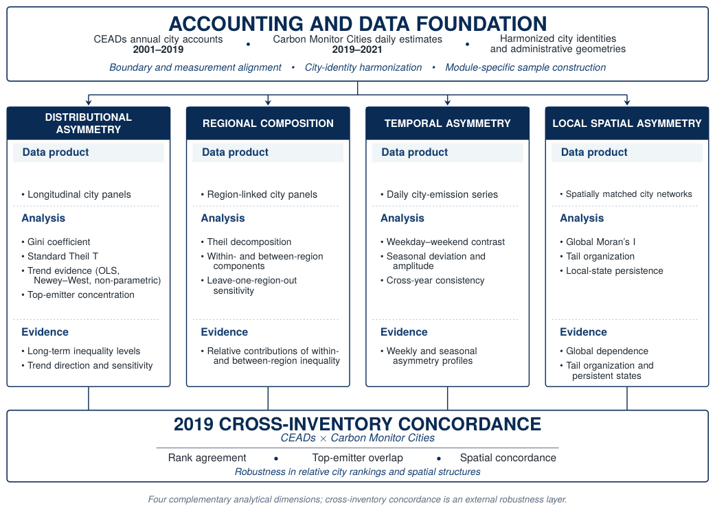
Figure 2.
Long-term evolution of city-level carbon-emission inequality from 2001 to 2019. Panel (A) presents annual Gini coefficients, and Panel (B) presents annual standard Theil T indices for the strict core and extended longitudinal samples. Dark navy lines represent the strict core sample, gray-blue dashed lines represent the extended sample, and muted teal lines show ordinary least-squares trends fitted to the corresponding core-sample observations. Both indicators exhibit negative fitted trends in the strict core sample, whereas their extended-sample slopes are positive and statistically non-significant, demonstrating sensitivity to longitudinal sample coverage.
Figure 2.
Long-term evolution of city-level carbon-emission inequality from 2001 to 2019. Panel (A) presents annual Gini coefficients, and Panel (B) presents annual standard Theil T indices for the strict core and extended longitudinal samples. Dark navy lines represent the strict core sample, gray-blue dashed lines represent the extended sample, and muted teal lines show ordinary least-squares trends fitted to the corresponding core-sample observations. Both indicators exhibit negative fitted trends in the strict core sample, whereas their extended-sample slopes are positive and statistically non-significant, demonstrating sensitivity to longitudinal sample coverage.
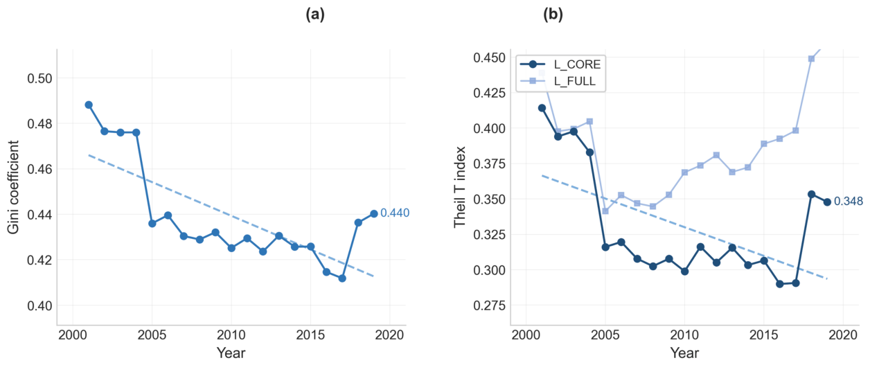
Figure 3.
Annual decomposition of standard Theil T inequality in the region-mapped longitudinal sample from 2001 to 2019. Each bar represents the annual total Theil T index, decomposed into within-region and between-region components. The within-region component exceeded the between-region component in every year and accounted for a median share of 96.0% of total inequality.
Figure 3.
Annual decomposition of standard Theil T inequality in the region-mapped longitudinal sample from 2001 to 2019. Each bar represents the annual total Theil T index, decomposed into within-region and between-region components. The within-region component exceeded the between-region component in every year and accounted for a median share of 96.0% of total inequality.
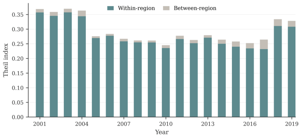
Figure 4.
Temporal asymmetry in daily city-level carbon emissions during 2019–2021. Panel (a) presents the median symmetric weekday–weekend asymmetry index for the pooled period and individual years. Panel (b) presents the absolute value of the cross-city median seasonal deviation from the corresponding annual mean, grouped by season and year. Plus and minus signs indicate seasonal emissions above and below the annual mean, respectively. Panel (c) reports the median seasonal amplitude, calculated from the highest- and lowest-emission seasonal means and normalized by the annual mean daily emission. The elevated 2020 values are interpreted descriptively rather than as evidence of a specific causal mechanism.
Figure 4.
Temporal asymmetry in daily city-level carbon emissions during 2019–2021. Panel (a) presents the median symmetric weekday–weekend asymmetry index for the pooled period and individual years. Panel (b) presents the absolute value of the cross-city median seasonal deviation from the corresponding annual mean, grouped by season and year. Plus and minus signs indicate seasonal emissions above and below the annual mean, respectively. Panel (c) reports the median seasonal amplitude, calculated from the highest- and lowest-emission seasonal means and normalized by the annual mean daily emission. The elevated 2020 values are interpreted descriptively rather than as evidence of a specific causal mechanism.
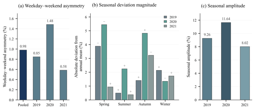
Figure 5.
Spatial asymmetry in city-level carbon emissions from 2001 to 2019. Panel (a) reports annual global Moran’s I values, with the dashed line marking the median annual value of 0.131. None of the annual tests remained significant after false-discovery-rate correction. Panel (b) summarizes the shares of years in which high–high connections were stronger than low–low connections, low–low connections were stronger than high–high connections, or neither tail strictly dominated. The corresponding numbers of years were 15, 3, and 1, respectively. Panel (c) compares the observed persistence probabilities of high–high and low–low local states with their matched conditional permutation-null means. The corresponding null distributions were generated using 2000 within-year label permutations that preserved annual marginal state frequencies. Error bars on the null means represent the central 95% ranges of the corresponding permutation-null distributions.
Figure 5.
Spatial asymmetry in city-level carbon emissions from 2001 to 2019. Panel (a) reports annual global Moran’s I values, with the dashed line marking the median annual value of 0.131. None of the annual tests remained significant after false-discovery-rate correction. Panel (b) summarizes the shares of years in which high–high connections were stronger than low–low connections, low–low connections were stronger than high–high connections, or neither tail strictly dominated. The corresponding numbers of years were 15, 3, and 1, respectively. Panel (c) compares the observed persistence probabilities of high–high and low–low local states with their matched conditional permutation-null means. The corresponding null distributions were generated using 2000 within-year label permutations that preserved annual marginal state frequencies. Error bars on the null means represent the central 95% ranges of the corresponding permutation-null distributions.
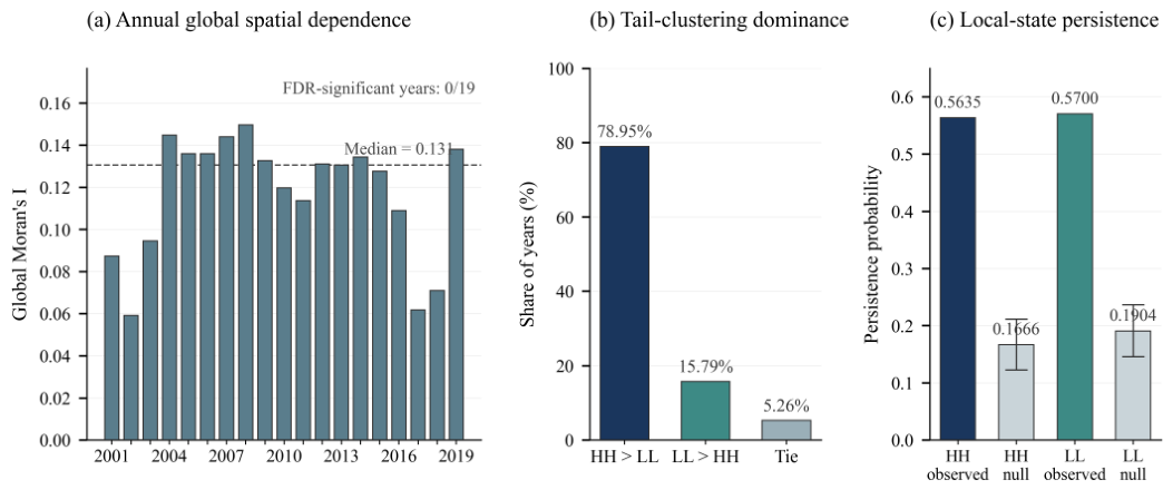
Figure 6.
Cross-inventory concordance in 2019 across city rankings, top-emitter identification, local spatial states, and neighbourhood patterns. Numerical estimates are reported in Table 5.
Figure 6.
Cross-inventory concordance in 2019 across city rankings, top-emitter identification, local spatial states, and neighbourhood patterns. Numerical estimates are reported in Table 5.
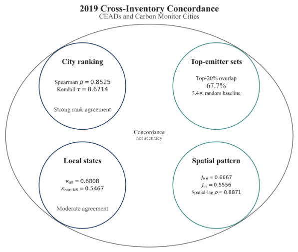

Table 1.
Analytical sample architecture.
| Sample | Coverage | Primary analytical role |
|---|---|---|
| 289 cities | Extended longitudinal sample used for robustness checks of long-term inequality trends. | |
| 72 cities | Strict core longitudinal sample used for annual inequality trends and local-state persistence. | |
| 56–65 cities/year | Region-mapped longitudinal sample used for the annual within-region and between-region Theil T decomposition. | |
| D | 311 cities | Daily Carbon Monitor Cities sample used for weekday–weekend and seasonal asymmetry analysis. |
| C | 158 cities | Strict 2019 CEADs–Carbon Monitor Cities matched sample used for non-spatial cross-inventory concordance. |
| 153 cities | Spatially eligible subset of C, used for comparing local spatial patterns across the two emission inventories. |
Notes: Fixed sample sizes refer to unique harmonized city identities. The entry for reports annual valid-city coverage because the number of region-mapped cities with observed emissions varies by year. Different samples are not assumed to have identical accounting boundaries or temporal resolutions. Of the 153 cities in , 140 had valid paired local Moran classifications in both inventories, and 103 were assigned a non- state by both sources, where denotes a non-significant local classification.
Table 2.
Long-term inequality levels and trend evidence for the strict core and extended longitudinal samples, 2001–2019.
Table 2.
Long-term inequality levels and trend evidence for the strict core and extended longitudinal samples, 2001–2019.
| Panel A. Main trend estimates | ||||
| Indicator | Sample (annual n) |
Median [min, max] |
OLS slope |
Newey–West p |
| Gini |
63–72 |
0.4306 [0.4119, 0.4882] |
0.0060 | |
| Gini |
106–263 |
0.4673 [0.4504, 0.4992] |
0.7177 | |
| Standard Theil T |
63–72 |
0.3155 [0.2899, 0.4142] |
0.0652 | |
| Standard Theil T |
106–263 |
0.3809 [0.3413, 0.4611] |
0.4255 | |
| Panel B. Non-parametric and sensitivity evidence | ||||
| Indicator | Sample | Theil–Sen slope |
Mann–Kendall (p) |
Leave-one-year-out OLS slope range |
| Gini | (0.0026) | [, ] | ||
| Gini | (0.2079) | [, ] | ||
| Standard Theil T | (0.0096) | [, ] | ||
| Standard Theil T | (0.0931) | [, ] | ||
Notes: Annual n reports the range of valid city counts across 2001–2019. OLS denotes the ordinary least-squares annual trend. Newey–West p-values use the canonical lag length of six and two-sided t-based inference. Leave-one-year-out ranges summarize OLS slopes after omitting one year at a time. Negative values indicate declining inequality, whereas positive values indicate increasing inequality. Trend estimates are sample-specific and should not be interpreted as nationally invariant trajectories.
Table 3.
Regional standard Theil T decomposition and leave-one-region-out robustness.
| Scenario | Within-region share (%) |
Between-region share (%) |
Change from all regions (pp) |
|---|---|---|---|
| All regions | 96.0 | 4.0 | — |
| Without Eastern | 94.8 | 5.2 | |
| Without Central | 95.5 | 4.5 | |
| Without Western | 96.8 | 3.2 | |
| Without Northeastern | 96.2 | 3.8 |
Notes: Entries report median shares across 2001–2019. “All regions” denotes the complete sample. Changes are reported in percentage points relative to the all-regions median within-region share.
Table 4.
Summary of weekday–weekend and seasonal emission asymmetry, 2019–2021.
| Analysis | Period | Estimate | 95% CI or criterion | Interpretation |
|---|---|---|---|---|
| Weekday–weekend asymmetry | ||||
| Pooled asymmetry | 2019–2021 | 0.0098 | 95% CI [0.0097, 0.0099] | Positive in all 311 cities; small magnitude |
| Annual asymmetry | 2019 | 0.0085 | 95% CI [0.0081, 0.0087] | Positive; small |
| Annual asymmetry | 2020 | 0.0148 | 95% CI [0.0145, 0.0151] | Largest annual contrast |
| Annual asymmetry | 2021 | 0.0058 | 95% CI [0.0057, 0.0059] | Positive; small |
| Seasonal asymmetry | ||||
| Seasonal amplitude | 2019 | 0.0926 | 95% CI [0.0860, 0.0983] | Moderate amplitude |
| Seasonal amplitude | 2020 | 0.1164 | 95% CI [0.1137, 0.1192] | Largest annual amplitude |
| Seasonal amplitude | 2021 | 0.0802 | 95% CI [0.0770, 0.0867] | Smallest annual amplitude |
| Seasonal consistency | 2019–2021 | 284/311 (91.3%) | Same highest-emission season in at least two years | Winter most frequently ranked highest |
Notes: The weekday–weekend asymmetry index is . Seasonal amplitude is the difference between the highest- and lowest-emission seasonal means divided by the annual mean daily emission. Confidence intervals are city-level percentile-bootstrap intervals based on 2000 replications. Peak-season recurrence denotes cities with the same highest-emission season in at least two of the three years.
Table 5.
Cross-inventory concordance between CEADs and Carbon Monitor Cities in 2019.
| Evidence dimension | Estimate | Comparator or additional information |
|---|---|---|
| Rank concordance | Spearman ; Kendall () | — |
| Top-emitter overlap | 67.7% () | Analytical random-set expectation: 19.6% |
| Global spatial dependence | ; () | |
| Local-state agreement | 75.0% (105/140); | Five-state paired classification |
| Conditional local-state agreement | () | Restricted to cities classified as non-NS in both inventories |
| Cluster-set overlap | ; () | HH and LL cluster-set concordance |
| Spatial-lag concordance | Spearman () | — |
Notes: CMC denotes Carbon Monitor Cities; NS denotes a non-significant local Moran classification. For the top-20% comparison, each inventory contributes the 31 highest-ranked cities (); under independent random assignment of two sets of this size, the expected overlap rate is . Concordance measures cross-inventory robustness and does not establish absolute accuracy.
Disclaimer/Publisher’s Note: The statements, opinions and data contained in all publications are solely those of the individual author(s) and contributor(s) and not of MDPI and/or the editor(s). MDPI and/or the editor(s) disclaim responsibility for any injury to people or property resulting from any ideas, methods, instructions or products referred to in the content. |
© 2026 by the authors. Licensee MDPI, Basel, Switzerland. This article is an open access article distributed under the terms and conditions of the Creative Commons Attribution (CC BY) license (http://creativecommons.org/licenses/by/4.0/).
Copyright: This open access article is published under a Creative Commons CC BY 4.0 license, which permit the free download, distribution, and reuse, provided that the author and preprint are cited in any reuse.


