

Submitted:
13 August 2026
Posted:
14 August 2026
You are already at the latest version
Abstract
Water lost from drinking-water distribution systems has already consumed electricity, yet the associated operational greenhouse gas burden is rarely quantified because water balances and organizational emission inventories use different system boundaries. This study links the two within the Greek managerial-adequacy framework using a purposive availability sample of eight utilities and 14 utility-year observations for reference years 2024–2025. We calculate water-supply energy intensity, operational electricity-related carbon intensity per cubic metre of system input (ISO 14064-1 Category 2), and emissions allocated to reported real losses. Because organizational inventories include activities outside water supply—fugitive wastewater emissions reach 94% of the declared total in one island municipality—we classify itemized electricity supply points by activity and grade attribution quality. Energy intensity ranges from 0.538 to 2.434 kWh/m³ and system-input carbon intensity from 0.198 to 0.895 kg CO₂eq/m³. Under proportional average-intensity allocation, reported real losses are assigned 22.0–67.5% of each utility’s water-supply electricity emissions and 2,708 t CO₂eq in the 2025 cross-section. These are accounting allocations from top-down water balances, not direct measurements of leak-specific energy use. A conditional screening analysis shows that, under a one-for-one production response and the illustrative unit-cost assumptions adopted here, leakage-reduction scenarios overlap selected European public-investment carbon-value benchmarks. The results support activity-level electricity reporting and joint consideration of leakage, energy intensity, and system scale when prioritizing mitigation.
Keywords:
non-revenue water
; water losses
; water–energy nexus
; carbon footprint
; ISO 14064-1
; IWA water balance
; emission attribution
; local climate planning
; marginal abatement cost
; Greece
1. Introduction
The transition to climate neutrality has shifted from the national to the local level. Municipalities operate emissions-generating infrastructure themselves—buildings, street lighting, vehicle fleets, waste and wastewater facilities, and water-supply and irrigation networks [1,2]. The European Covenant of Mayors has produced emission inventories for more than six thousand cities [3], while a critical review of 257 local action plans shows that they remain weak in infrastructure-specific detail [4]. In Greece, National Climate Law 4936/2022 made the preparation of a Municipal Emission Reduction Plan (MERP) and annual progress reporting mandatory for every municipality [5]; by August 2025, only 44% of municipalities had commissioned one [6].
Within this context, water supply occupies a peculiar position. It is among the most energy-hungry municipal activities, since abstraction, conveyance, treatment and distribution all require continuous electricity input [7,8,9]. The international literature documents a wide range of energy intensities for urban water systems, with the pumping of finished water representing 80–85% of total supply energy in large metropolitan systems [10], while in small-scale utilities energy can reach 44% of operating costs [11]. At the same time, water supply is rarely treated as a mitigation sector in its own right in local climate planning: a comparative assessment of three Greek MERPs found that whether a municipality runs its own water service or has delegated it materially changes the reported footprint, without this being reflected in target-setting [12].
Climate adds to the pressure. The Mediterranean is warming rapidly, water resources are under sustained stress, and dry spells are projected to intensify [13]. At the European scale, compound warm-season droughts—those combining precipitation deficit with heat stress—have increased markedly over recent decades, with the Mediterranean among the most exposed regions [14]. On the Greek islands, hydrometeorological trend analysis shows stagnant precipitation combined with statistically significant warming, indicating growing aridity through evapotranspiration [15], while the tourist peak multiplies demand precisely when availability is lowest [16,17]. On many islands, the response is desalination, whose specific energy consumption shifts part of the resource problem to energy use and emissions [18,19,20,21]. Adapting water infrastructure to these pressures has been recognized for a decade as a matter of operational readiness rather than planning alone [22]. Heatwaves also coincide with peak water demand and high electrical loads in desalination-dependent systems, making water and energy interlinked risks [23].
The other side of the problem is losses. Worldwide, an estimated 126 billion m³ of water is lost each year, at a cost on the order of USD 39 billion [24], and a recent pan-European survey shows that non-revenue water (NRW) remains high and strikingly uneven across Member States [25]. The order of magnitude of the problem was already recognized in the first global estimates of the 2000s [26]. In Greece and the wider Mediterranean, measurements in DEYA networks and island systems consistently show high loss rates [27,28,29], while the structural determinants of losses—governance model, service type, network length—have been documented in long-run Iberian data [30,31]. Water that leaves the distribution system without authorized use has nonetheless been abstracted, lifted, possibly desalinated and disinfected; that energy has been spent and the corresponding emissions released. At the same time, lost water is a cost that tariffs do not recover, in direct conflict with the full cost recovery principle of Article 9 of the Water Framework Directive [32,33], whose application remains uneven in the absence of a standardized methodology for environmental cost [34].
Despite the intuitive clarity of the point, explicit quantification remains uncommon. The water–energy–emissions nexus literature has developed the conceptual framework [35] and documented that hydraulic losses are also an energy inefficiency [36,37]. As early as 2002, Colombo and Karney showed that energy spent on leaking water is a measurable and often underestimated system cost [38], while Greek work framed the techno-economic relationship between leaks and breaks as an optimal pipe-replacement problem [39]. Only a limited number of studies proceed to explicit emissions attribution: Muhammetoglu et al. assign 35.4% of supply-stage energy and emissions to physical losses in a Mediterranean system [40]; Korean and Polish studies isolate 6,979 and approximately 2,808 t CO₂eq per year, respectively [41,42]; and a study of ten U.S. cities reports 21–560 g CO₂eq/m³ and converts saved water into avoided emissions [43]. One related Greek study converts leakage reduction at a Patras pumping station into avoided CO₂ [44]. In parallel, the international water-utility community has begun to standardize the process through the Leakage Emissions Initiative [45].
The remaining gap is primarily methodological. Attributing emissions to losses requires three elements for the same system and year: a standardized water balance, an emission inventory compiled to a recognized standard, and—critically—the ability to isolate the inventory component corresponding to water supply. The third element is usually missing. Local-government inventories are compiled for the organization rather than the service, and fugitive methane and nitrous oxide emissions from wastewater treatment can dominate the total [46,47,48]. Dividing a municipality’s total emissions by water volume therefore yields a non-service-specific ratio that may be severely biased.
Greece offers an unusual opportunity to resolve this. Under Law 5037/2023, the Regulatory Authority for Energy was renamed the Regulatory Authority for Waste, Energy and Water (RAAEY) and acquired competence over water services [49,50]. As part of the managerial adequacy assessment, every provider must submit a single documentation dossier including, among other items, an IWA water balance, a leakage assessment, a carbon footprint report and cost recovery data, using common templates and a common reference year [51,52]. This produces, for the first time in Greece, a nationally harmonized—though not yet representative in coverage—dataset in which the water and carbon strands coexist per utility.
This paper uses that dataset to address three research questions:
- (RQ1) Can the emission inventories reported by Greek providers be used directly to calculate the carbon intensity of water and, if not, how large an error does unattributed use introduce?
- (RQ2) What are the energy and operational carbon intensities per cubic metre of system input in Greek utilities, and how do they vary by system type?
- (RQ3) What operational emissions are allocated to reported real losses, and under what explicit unit-cost and production-response conditions can leakage reduction overlap selected carbon-value benchmarks?
The paper makes three contributions. First, it proposes and applies a transparent protocol for attributing an organization’s emissions to the water-supply service, with an explicit quality grade that can be embedded in existing regulatory reporting. Second, it provides descriptive estimates of operational water-supply carbon intensity and emissions allocated to reported real losses for Greek utilities. Third, it places leakage reduction in a conditional cost-screening framework using the EU ETS allowance price and selected European public-investment carbon-value benchmarks [53,54,55,56]. The contribution is descriptive and methodological; national representativeness, causal typology inference, and utility-specific project appraisal remain outside the scope of the available data.
2. Materials and Methods
2.1. The Managerial Adequacy Regulatory Framework
The Greek water services market is fragmented. Water supply is provided by Municipal Water Supply and Sewerage Companies (DEYAs), municipal departments, the two large companies of Athens and Thessaloniki, and Land Reclamation Organizations for irrigation [57,58]. This heterogeneity has historically hindered systematic benchmarking, even after the mergers of the “Kallikratis” reform [59].
Law 5037/2023 changed this picture. Its Article 12 inserted Articles 12A and 12B into Law 4001/2011, establishing the managerial adequacy regime and assigning its assessment to RAAEY [49]. Joint Ministerial Decision ΥΠΕΝ/ΔΣΔΥΥ/53924/460/2023 set out the criteria and the procedure [51], while RAAEY’s Guide for the preparation of the documentation dossier standardized the templates and the dossier structure [52]. Every provider submits a single dossier annually, covering, among other items: a technical description of the network, an IWA-standard water balance, a leakage assessment using the WB-EasyCalc software, a carbon footprint report using the YPEN calculation tool, cost recovery and tariff policy data, and staffing data.
The three core technical volumes—water balance, leakage assessment, carbon footprint—are prepared with common templates, by the same organization, for the same reference year, and form a single harmonized regulatory submission. This is the property that makes it possible to link water accounting to carbon accounting within the same system.
2.2. Sample and Data
The retained dataset consists of documentation dossiers available to the research team for eleven providers and reporting reference years 2024 and/or 2025. The year labels denote the year to which the water and inventory data refer, not a random sampling wave. Availability of a complete water balance was the entry condition for the retained set: all eleven providers meet it, ten also have an emission inventory, and eight meet the additional requirement that electricity can be attributed to water supply. These eight utilities yield 14 analytical utility-year observations. No provider outside the retained set was screened and excluded. The resulting sample is therefore purposive and availability-based, not random or nationally representative. The eight analytical utilities cover 134,701 permanent residents and approximately 19.1 million m³ of 2025 system input. Cross-sectional totals and weighted indicators use one observation per utility (2025); the six available 2024 observations are used only for descriptive year-to-year comparison. Permanent population is taken from the 2021 census [60]. A utility-level inclusion and data-quality matrix is provided in the Supplementary Material.
The sample spans three distinct system types: small and medium Aegean and Sporades islands (Fournoi Korseon, Alonnisos, Lemnos), mountainous and semi-mountainous mainland interior (Souli, Dorida), and medium-sized mainland DEYAs and municipalities in coastal lowland areas (Corinth, Trifylia, Aktio-Vonitsa). The size range is wide: from 1,343 permanent residents in Fournoi to 55,941 in Corinth, and from 0.20 to 5.9 million m³ of annual system input. These utilities fall within the “small and medium systems” category, for which the literature has documented particular governance, staffing and benchmarking challenges [61,62].
Two providers with a water balance (Chios, Sifnos) and the Municipality of Leros are not part of the analytical sample: the first two because they report aggregate electricity metering, the third because it has not submitted an emission inventory. They are nevertheless shown in the analysis of Section 3.1, precisely because the impossibility of attribution is itself a finding.
2.3. The IWA Water Balance
The water balance follows the standard International Water Association scheme [63,64,65,66]. System Input Volume (SIV) is split into authorized consumption and water losses; authorized consumption into billed and unbilled, metered and unmetered; and losses into apparent (unauthorized consumption and metering errors) and real (leakage on mains, leakage and overflows at storage tanks, leakage on service connections up to the meter). Non-revenue water is defined as the sum of losses and unbilled authorized consumption.
The distinction between apparent and real losses is essential for this analysis. Apparent losses correspond to water that was consumed but not properly billed; the energy for its production was not physically wasted, although it was not recovered financially. Reported real losses, by contrast, represent water estimated to have left the distribution system without authorized use after abstraction, conveyance, and treatment. This distinction, and the uncertainty attached to top-down loss estimation, is extensively documented [67,68,69,70]. The core allocated-carbon indicator uses reported real losses, while the corresponding indicator for total NRW is shown as an upper-bound accounting allocation.
Utilities also calculate loss performance indicators with the WB-EasyCalc software [71]—one of the tools that have been comparatively assessed for their treatment of uncertainty and the consistency of the indicators they produce [72]—yielding current annual real losses (CARL), unavoidable annual real losses (UARL) and the Infrastructure Leakage Index (ILI) [73,74].
2.4. The ISO 14064-1 Emission Inventory
The carbon footprint is calculated with the YPEN tool, which, according to its documentation, implements ISO 14064-1:2018 in combination with the Global Protocol for Community-Scale Greenhouse Gas Inventories and the IPCC guidelines [75,76,77]. Emissions are classified into Category 1 (direct emissions, including fugitive CH₄ and N₂O emissions from wastewater treatment and disposal) and Category 2 (indirect emissions from imported electricity consumption). All gases are expressed in carbon dioxide equivalent using the global warming potential factors (GWP₁₀₀) that the YPEN tool embeds for CH₄ and N₂O [77].
The analytical recalculation uses 367.51 g CO₂/kWh, the 2024 residual-mix factor published for the Greek system by DAPEEP [78]. Because the factor refers to CO₂, its numerical value is unchanged when the resulting inventory quantity is reported in CO₂-equivalent units. The factor is held constant across the 2024 and 2025 observations to isolate utility changes from changes in the grid mix. DAPEEP published a 2025 value of 360.3426 g CO₂/kWh [79]; the difference (−2.0%) is examined in the uncertainty analysis of Section 2.8. One retained utility outside the analytical subsample (Sifnos, 2025) used the 2025 factor in its submitted inventory.
2.5. Protocol for Attributing Emissions to Water Supply
Inventories are compiled at the level of the organization, not the service. The declared total may cover street lighting, buildings, the vehicle fleet, irrigation, waste management, and fugitive emissions from wastewater treatment. The latter can be substantially larger than water-supply electricity emissions because they arise from biochemical processes rather than electricity use [46,48]. Dividing the organizational total by the volume of water supplied therefore does not produce a service-specific intensity. This is a system-boundary issue rather than an error in the submitted inventory; the itemized electricity data can, where sufficiently detailed, be used to resolve it.
The solution rests on subcategory 2.1 of the YPEN tool, where electricity consumption is recorded per supply point (per meter number of the electricity provider), with a description of the installation served. The proposed protocol, shown schematically in Figure 1, has four steps:
- Extraction of the itemized subcategory 2.1 entries and of the description of each supply point.
- Classification of each supply point into one of four classes: (a) water supply, covering boreholes, water pumping stations, storage tanks, desalination units and drinking-water treatment plants; (b) sewerage and wastewater treatment; (c) irrigation; and (d) other municipal uses, including street lighting and buildings. A fixed descriptor dictionary is applied first. Explicit activity terms take precedence; mixed-use or shared-meter descriptions are not forced into a single class; and descriptions that remain ambiguous after checking the dossier are retained as unclassified. The first author performed the coding and manual verification. The process was not independently double-coded. The dictionary, precedence rules, and verification record are provided in the Supplementary Material.
- Summation of class (a) energy into E_w (kWh/year) and conversion into emissions using the emission factor EF.
- Grading of attribution quality at three levels: Full, when every supply point is classifiable and class totals reconcile with the declared electricity total within the rounding precision of the submitted tool; Partial, when a shared, mixed-use, or otherwise unclassifiable residual remains; and None, when electricity is reported only as one organizational aggregate.
The grade describes attribution granularity, not the accuracy of meter labels or the physical completeness of the inventory. Full observations enter the analysis at the classified water-supply value. Partial observations enter as lower-bound allocations, with the residual quantified separately and its service mix left unresolved. Utilities graded None are excluded from intensity indicators irrespective of the quality of their water-balance data.
2.6. Derived Indicators
Based on the above, the following indicators are defined. The energy intensity per cubic metre of system input is:
EI = Ew / SIV [kWh/m3]
The energy emissions of water supply:
Cw = Ew · EF / 106 [t CO2eq/yr]
The operational electricity-related carbon intensity per cubic metre of system input is:
CI = Ew · EF / (103 · SIV) [kg CO2eq/m3]
The carbon attributable to real losses and to non-revenue water:
CRL = CARL · CI / 103 ; CNRW = NRW · CI / 103 [t CO2eq/yr]
The share of water supply energy emissions attributable to losses:
sRL = CRL / Cw = CARL / SIV
Equation (5) is an accounting identity: under proportional average-intensity allocation, the assigned emissions share is numerically equal to the reported real-loss fraction. It is not an independent empirical relationship or a direct measurement of the energy used by individual leaks. The absolute allocation depends on the product of loss fraction, average energy intensity, and system input; two utilities with the same loss fraction can therefore differ substantially in assigned emissions.
Finally, for comparison, a naive organizational-total-to-system-input ratio is defined using the declared total emissions C_tot:
where r is the organizational-boundary-mismatch factor. CI* is the organizational total divided by SIV and is reported only to quantify the error produced when that ratio is interpreted as a water-supply indicator. Thus r measures mismatch relative to the electricity-only service indicator CI; it does not compare CI with a full life-cycle water-service footprint. All other indicators refer solely to operational emissions from imported electricity (ISO 14064-1 Category 2) using a residual-mix factor and exclude embodied, construction, chemical, and other life-cycle emissions. Below, ‘carbon intensity’ and emissions ‘allocated’ to losses always refer to this operational electricity boundary.
CI* = Ctot · 103 / SIV ; r = CI* / CI
2.7. Conditional Marginal Abatement Cost Screening
A conditional marginal abatement cost (MAC) calculation is used as a screening device, not as project appraisal. Let I be the levelized intervention cost per cubic metre of system input avoided through leakage reduction (€/m³) and c the corresponding avoidable variable production cost (€/m³). The formulation assumes, as a first-order production response, that one cubic metre of verified leakage reduction permits one cubic metre less system input. Under that assumption, the net cost of avoiding one tonne of CO₂eq is:
MAC = (I − c) · 103 / CI [€/t CO2eq]
When I < c, MAC is negative: the intervention yields a net economic benefit regardless of the value of carbon. The intervention cost at which carbon avoidance is valued at a given price p (€/t) follows from:
I*(p) = c + p · CI / 103
Only three comparable WB-EasyCalc financial sheets were available in the retained provider set (Souli, Chios, and Sifnos). Their variable production-cost values span 0.20–0.60 €/m³, with Chios between the endpoints. This range is broadly consistent with the 0.09–0.51 €/m³ European range reported in the literature [80] and with loss valuations recorded for Mediterranean countries [81]. Because three observations do not support a sample distribution, c = 0.33 €/m³ is used only as a common central scenario and the full 0.20–0.60 €/m³ retained range is tested. The mean selling-price range in the retained utilities (0.93–2.30 €/m³) is contextual and is not substituted for avoidable cost; it is consistent with the national tariff survey of eighty-four DEYAs [82]. Monetary quantities are expressed in 2024 prices.
The unit intervention cost I remains a scenario variable because it depends on intervention type, network condition, asset life, discount rate, and verified reduction in system input. Published infrastructure-unit costs—48,000 € per district metered area, 9,000 € per pressure-reducing valve, and 94–628 € per metre of pipe rehabilitation [80]—cannot be converted to €/m³ avoided without project-specific engineering and financial assumptions. The analysis therefore varies I and uses 0.40 €/m³ only as an illustrative reading point. Internal consistency requires I to be levelized over the same real-price and time basis as the stream of verified avoided production costs and emissions. This annual screening does not model asset-specific lifetimes or discounting, future grid decarbonization, intervention embodied emissions, rebound, pressure-dependent demand, or a utility-specific marginal leakage-reduction curve. The cost c must represent genuinely avoidable energy, chemicals, or purchased water; inclusion of fixed costs would overstate the benefit. Results are conditional scenario comparisons, not estimates of optimal investment or bankable project returns.

Table 2.
Parameters for the conditional marginal abatement cost screening.
| Screening parameter | Value | Source / note |
|---|---|---|
| Variable production cost, c | 0.20–0.60 €/m³ (central scenario 0.33) | WB-EasyCalc financial sheets available within the retained provider set |
| European range of marginal water cost | 0.09–0.51 €/m³ | Ahopelto & Vahala (2020) |
| Levelized intervention cost per m³ of system input avoided, I | variable, levelized (indicatively 0.40 €/m³) | Scenario parameter; no directly comparable Mediterranean estimate identified |
| Mean EUA price, 2024 (external benchmark) | 65 €/t CO₂eq | ESMA, EU Carbon Markets 2025 |
| CINEA shadow-carbon benchmark, 2026 | 229 €/t CO₂eq (2024 prices; 182 €/t in 2016 prices) | CINEA Guide for CEF Transport appraisal [54]; uprated using Eurostat HICP [56] |
| CINEA shadow-carbon benchmark, 2030 | 315 €/t CO₂eq (2024 prices; 250 €/t in 2016 prices) | Ibid. |
| National Greek shadow-carbon value | not identified | No water-sector value identified; external benchmark used |
| Electricity emission factor, EF | 367.51 g CO₂/kWh | Residual mix of the Greek system, DAPEEP 2024 |
Two external carbon-value references are used. The first is the mean 2024 EU Emissions Trading System allowance price, 65 €/t [83]. It is a market benchmark only: water utilities are not covered by the ETS, so an avoided tonne does not create a corresponding receipt. The second is the shadow-carbon series in the CINEA Guide on Economic Appraisal for CEF Transport Projects: 182 €/t for 2026 and 250 €/t for 2030, expressed in 2016 prices [54]. These values are used as external public-investment benchmarks, not as water-sector tariffs or mandatory appraisal values. Uprating them to 2024 prices with the euro-area HICP factor of 1.26 gives 229 €/t and 315 €/t [56]. No national Greek shadow-carbon value for water investment appraisal was identified; the benchmark comparison is therefore illustrative.
2.8. Uncertainty and Data Limitations
The sources of uncertainty are acknowledged explicitly and quantified where feasible.
First, reported real losses are generally top-down balance residuals, and their internal component splits often follow standardized apportionment ratios rather than minimum-night-flow or leak-level measurement. The resulting C_RL values are therefore accounting allocations to estimated real losses, not direct measurements of leakage emissions. Comparative studies show that top-down and bottom-up methods can diverge substantially, particularly in intermittently supplied systems [67,68].
Second, unauthorized consumption and meter errors are estimated through assumptions. Since the paper’s core indicator is defined on real rather than total losses, sensitivity here is limited; the C_NRW indicator is reported as an upper bound.
Third, reconciliation checks identified inconsistencies between declared abstraction at source, external-network losses, and SIV; external-network figures were therefore not used. The SIV identity against authorized consumption, apparent losses, and real losses was also checked. For Souli, the authorized-consumption entry was reconciled arithmetically to 772,940 m³ (= SIV − apparent losses − real losses); this does not change CARL, NRW, or any downstream energy and carbon result. After this reconciliation, SIV is internally consistent with the balance components used in all observations.
Fourth, the core indicators are recalculated under a low–central–high sensitivity band. Reported real losses are varied by ±20%, while the emission factor takes the published residual-mix values of 360.34 (2025) and 367.51 g CO₂/kWh (2024) [78,79]. The ±20% interval is an analyst-defined stress test, not a confidence interval or a provider-specific error bound. It yields 2,125–3,250 t CO₂eq per year across the eight utilities, against the central 2,708 t. This sensitivity is distinct from the marginal-response test in Section 3.6 and the two ranges should not be combined. For Partial attribution, the unclassified residual is 0.26 GWh in Dorida (8.2% of 3.16 GWh) and 0.28 GWh in Alonnisos (42.3% of 0.67 GWh), so their E_w, EI, and CI are lower-bound allocations. Assigning the entire residual to water supply would raise EI from 1.293 to 1.507 kWh/m³ and CI from 0.475 to 0.554 kg CO₂eq/m³ in Dorida, and EI from 0.922 to 1.702 kWh/m³ and CI from 0.339 to 0.626 kg CO₂eq/m³ in Alonnisos. Allocated loss emissions would rise from 146 to 170 t and from 67 to 124 t, lifting the sample total by 3.0% to 2,789 t CO₂eq. This is a conservative upper allocation because the residual’s actual service mix is unknown. Fifth, Fournoi submitted identical 2024 and 2025 values in both the water balance and inventory. The observation is retained because the submitted figures reconcile, but is treated as one independent case in year-to-year interpretation.
Finally, the sample size (eight utilities) supports descriptive and comparative analysis but not inferential statistics. The 14 utility-year observations are not independent because six utilities contribute two years, and Fournoi reports identical values in both years. Differences between island and mainland utilities are therefore presented as observations, not as statistically established relationships.
3. Results
3.1. The Attribution Problem
Figure 2 shows the composition of the declared emissions of the ten utilities with an inventory, for 2025. The picture is highly heterogeneous and does not track utility size. The Municipality of Fournoi Korseon, with 1,343 permanent residents, declares total emissions of 4,563 t CO₂eq—more than the DEYA of Trifylia (2,442 t) and comparable to the DEYA of Corinth (4,711 t), which serves a forty times larger population. The explanation lies in the composition: in Fournoi, fugitive methane and nitrous oxide emissions from wastewater management amount to 4,279 t CO₂eq, or 94% of the declared total. Category 2 emissions, which cover the municipality’s entire electricity consumption, come to just 221 t CO₂eq.
Lemnos, Dorida, Trifylia, and Sifnos show the same pattern in weaker form: fugitive emissions account for 69%, 58%, 43%, and 33% of their totals, respectively. At the other end, Aktio-Vonitsa, Souli, and Alonnisos report zero or near-zero fugitive emissions. This may reflect the absence of a wastewater plant, exclusion of wastewater management from the reporting boundary, or inventory assumptions; the submitted totals alone do not distinguish among these explanations. The 0–94% range within a common framework shows that organizational totals primarily reflect institutional service boundaries and should not be interpreted as water-supply energy-performance indicators.
Figure 3 maps attribution quality. Of the ten utilities with an inventory, six achieve Full attribution in 2025 (Aktio-Vonitsa, Fournoi, Corinth, Souli, Trifylia, Lemnos), two Partial (Dorida, Alonnisos) and two None (Chios, Sifnos). Alonnisos improved from None in 2024 to Partial in 2025, which shows that the transition is feasible without legislative intervention, simply through more detailed recording. In total, two of the ten utilities report a single aggregate supply point for all municipal activities in 2025—three, counting Alonnisos in 2024—making any water intensity indicator impossible to compute. This concerns 9.2 GWh (Chios) and 0.64 GWh (Sifnos) of annual consumption that cannot be linked to any specific service.
Figure 4 shows how electricity consumption is distributed in the attributed utilities. The water-supply share ranges from 48.9% (Aktio-Vonitsa) to 89.1% (DEYA Corinth), with other utilities between these values (Table 3). The variation plausibly reflects the breadth of each organization’s responsibilities: specialized DEYAs tend to show higher shares, whereas municipal inventories also include street lighting and buildings. This reinforces the need for activity-level attribution before comparing organizations with different institutional boundaries.
3.2. The Effect of Attribution on System-Input Carbon Intensity
Figure 5 and Table 4 compare attributed system-input carbon intensity with the organizational-total-to-SIV ratio. The resulting organizational-boundary-mismatch factor r ranges from 1.4 to 25.3.
At DEYA Corinth, where water supply absorbs 89% of electricity and fugitive emissions are limited, the organizational ratio (0.798 kg CO₂eq/m³) exceeds the attributed estimate (0.557) by 43%. In Fournoi, the corresponding values are 22.63 and 0.895 kg CO₂eq/m³, a boundary-mismatch factor of 25.3. Interpreting the organizational ratio as drinking-water intensity would therefore be misleading; the attributed electricity-only estimate, although the highest in the sample, remains comparable in order of magnitude to values reported for island and small systems [62,84].
Intermediate factors occur in Dorida (×5.7), Lemnos (×5.7), Aktio-Vonitsa (×2.9), Alonnisos (×2.8), Souli (×2.2), and Trifylia (×2.1). All else equal, r decreases mechanically as the water-supply share of organizational electricity rises; fugitive and other non-electricity emissions increase it further. It is therefore an indicator of boundary mismatch, not of hydraulic or energy performance.
A service-specific system-input carbon intensity can therefore be calculated only after attribution. Without attribution, the same arithmetic produces non-comparable values that may differ by more than an order of magnitude. The required itemized electricity information already exists in most submitted tools; the remaining requirement is consistent activity classification.
3.3. Water Balance and Losses
Figure 6 and Figure 7 show the 2025 water-balance composition and loss percentages for all eleven utilities. Leros is retained in both views; the repeated internal apportionment of its real-loss subcomponents is treated as a data-quality limitation, not as a basis for omitting its aggregate real-loss estimate.
NRW ranges from 26.7% (Fournoi) to 71.1% (Aktio-Vonitsa). The unweighted arithmetic mean across the eleven utilities is 46.2%, while the aggregate volume-weighted ratio ΣNRW/ΣSIV is 47.0%. Reported real losses range from 22.0% to 67.5% of system input. Apparent losses are relatively uniform, between 2.7% and 7.6%, which likely reflects the standardized estimation method as well as any genuine metering differences. Chios reports four hours of supply per day. Intermittent supply can increase failures through network loading cycles [85] and makes top-down loss estimates less reliable [68].
Two utilities exceed 60% real losses—Aktio-Vonitsa (67.5%) and Leros (60.5%)—and a third approaches that level (Alonnisos, 54.7%). For Aktio-Vonitsa this means that of the 5.10 million m³ entering the network, only 1.47 million m³ is billed. These values are high even by European standards [25] and are in line with earlier findings in Greek and Cypriot networks [27,28].
The ILI, where calculated, produces a ranking different from NRW. Souli, with NRW of 40.9%, reports an ILI of 1.25 because its average operating pressure of 60 m and long mains length per connection lead to a comparatively high modeled UARL. Sifnos, with NRW of 53.0%, reports an ILI of 2.28, while Chios, with NRW of 38.9%, reports an ILI of 11.06. This divergence is well documented: ILI and percentage indicators measure different aspects of performance, and substituting one for the other can misrank utilities [73,86,87]. The choice of indicator therefore affects intervention priorities, although a full comparison is outside the scope of this paper.
Table 5.
IWA water balance, year 2025.
| Utility | SIV (m³/year) |
Authorized consumption (m³) |
Apparent losses (m³) |
Real losses (m³) |
Real (% SIV) |
NRW (m³) |
NRW (% SIV) |
|---|---|---|---|---|---|---|---|
| Aktio-Vonitsa | 5,096,115 | 1,521,854 | 135,277 | 3,438,984 | 67.5 | 3,625,222 | 71.1 |
| Alonnisos | 361,018 | 136,057 | 27,370 | 197,591 | 54.7 | 228,571 | 63.3 |
| Dorida | 1,207,440 | 847,941 | 52,250 | 307,249 | 25.4 | 371,574 | 30.8 |
| Corinth | 5,906,214 | 3,668,739 | 312,341 | 1,925,134 | 32.6 | 2,373,002 | 40.2 |
| Lemnos | 1,827,900 | 994,131 | 106,883 | 726,887 | 39.8 | 845,769 | 46.3 |
| Souli | 1,287,740 | 772,940 | 69,480 | 445,320 | 34.6 | 527,300 | 40.9 |
| Trifylia | 3,222,224 | 2,258,331 | 144,722 | 819,171 | 25.4 | 985,308 | 30.6 |
| Fournoi | 201,610 | 151,752 | 5,506 | 44,352 | 22.0 | 53,890 | 26.7 |
| Chios | 4,229,898 | 2,712,322 | 191,758 | 1,325,818 | 31.3 | 1,644,499 | 38.9 |
| Sifnos | 553,500 | 304,425 | 24,908 | 224,168 | 40.5 | 293,355 | 53.0 |
| Leros | 1,419,650 | 496,878 | 64,594 | 858,178 | 60.5 | 943,507 | 66.5 |
SIV: system input volume. NRW: non-revenue water. Leros has no emission inventory and is excluded from the intensity analysis. For Souli, authorized consumption is the reconciled value SIV − apparent losses − real losses (772,940 m³); the loss quantities used in downstream calculations are unchanged.
3.4. Energy and Carbon Intensity per Cubic Metre of System Input
Figure 8 and Figure 9 present the energy and carbon intensities of the eight utilities in the analytical sample.
Energy intensity ranges from 0.538 kWh/m³ (Aktio-Vonitsa) to 2.434 kWh/m³ (Fournoi), with a system-input-weighted mean of 1.061 kWh/m³. Dossier descriptions indicate that Aktio-Vonitsa and Lemnos rely comparatively more on gravity or low-lift supply, whereas Fournoi, Souli, and Corinth have pumping-intensive or desalination-related infrastructure. Souli’s dossier records seventy-five pumping stations, boreholes, and tanks across 502.8 km² with substantial elevation differences. These descriptors provide context only: hydraulic head, source mix, and pump efficiency were not independently measured as explanatory covariates.
Against the 0.4–0.9 kWh/m³ range reported for distribution in developed urban systems [8,10], six of the eight utilities exceed 0.9 kWh/m³. This comparison is indicative rather than like-for-like because published studies differ in process boundary, denominator, treatment level, source type, and reporting year. Geomorphology, settlement dispersion, and small scale are plausible explanations identified in the literature [62,88], but the present sample does not estimate their causal effects.
System-input carbon intensity, calculated with a common residual-mix factor, ranges from 0.198 to 0.895 kg CO₂eq/m³, with a system-input-weighted mean of 0.390 kg CO₂eq/m³. The values are higher than those reported for Seoul (0.11–0.13 kg CO₂/m³) [10] and overlap or exceed the 0.021–0.560 kg CO₂eq/m³ range reported for ten large U.S. cities [43]. Direct comparison remains indicative because electricity mix, hydraulic boundary, treatment stages, and denominators differ across studies [89,90,91]. Similar orders of magnitude have been reported for Scottish island systems [84] and a high-unbilled-water Mediterranean system in Madeira [92].
Figure 10 combines energy intensity with the reported real-loss fraction. No clear monotonic pattern appears in this small sample: Aktio-Vonitsa and Alonnisos have the highest loss fractions but comparatively low energy intensity, while Fournoi has the lowest loss fraction and the highest intensity. This illustrates why loss percentage alone is insufficient for climate prioritization. The pattern is consistent with probabilistic work on intermittent systems, in which increasing losses from 10% to 30% changed total system energy by 15–16% [93], although the system boundaries are not identical.
The three island utilities have a mean energy intensity of 1.315 kWh/m³, compared with 1.173 kWh/m³ for the five mainland utilities; their corresponding mean carbon intensities are 0.483 and 0.431 kg CO₂eq/m³. With n = 3 and n = 5 and large within-group dispersion, these are descriptive contrasts only. Dossier metadata suggest that supply mode (gravity, pumping, or desalination) may be more informative than insularity alone, but this hypothesis requires a larger sample with measured hydraulic and source-mix covariates.
3.5. Emissions Allocated to Reported Real Losses
Under proportional average-intensity allocation, the eight-utility 2025 cross-section assigns 2,708 t CO₂eq to reported real losses and 3,175 t CO₂eq to total NRW as an upper-bound indicator. The real-loss allocation corresponds to 7.37 GWh and 12.3% of the eight organizations’ combined declared emissions. These quantities describe an accounting allocation within the electricity boundary; they are not leak-level measurements of energy consumption.
For individual utilities, the assigned share ranges from 22.0% (Fournoi) to 67.5% (Aktio-Vonitsa) and equals the reported real-loss fraction by the identity in Equation (5). Across the sample, ΣC_RL/ΣC_w is 36.3%, an emissions-weighted allocation that should not be confused with the aggregate volume ratio ΣCARL/ΣSIV = 41.4%. The informative cross-utility differences are therefore in energy intensity, carbon intensity, and absolute quantities. The 36.3% value is numerically close to the 35.4% reported for one Mediterranean system [40], but differing boundaries and methods preclude interpreting proximity as validation.
Absolute rankings differ. Corinth receives the largest allocation (1,072 t CO₂eq) despite a lower loss fraction than several utilities, because it combines substantial system input (5.91 million m³) with high average energy intensity (1.515 kWh/m³). Aktio-Vonitsa follows at 680 t, while Fournoi combines the highest carbon intensity per cubic metre with the smallest absolute allocation. Intensity and quantity therefore identify different priorities.
Figure 12 illustrates the calculation for Aktio-Vonitsa. Of 5.10 million m³ of system input, 1.52 million m³ is authorized consumption, 0.14 million m³ apparent losses, and 3.44 million m³ reported real losses. Applying the system-average energy intensity of 0.538 kWh/m³ allocates 1.85 GWh and 680 t CO₂eq to reported real losses, equal by construction to 67.5% of water-supply electricity emissions.
Figure 13 generalizes the accounting relationship. Allocated emissions per cubic metre of system input equal the product of reported real-loss fraction and average carbon intensity, so similar values can arise from different combinations. Fournoi combines 22.0% reported real losses with 2.434 kWh/m³, whereas Aktio-Vonitsa combines 67.5% with 0.538 kWh/m³. Their technical profiles differ even where the assigned burden per unit of system input is similar.
3.6. Conditional MAC Screening and Reduction Scenarios
Figure 14a presents the conditional MAC screening curves for the eight utilities, using levelized cost per cubic metre of system input avoided as the horizontal variable and c = 0.33 €/m³. Under the one-for-one production-response assumption, every curve crosses zero at I = c by definition. Different slopes reflect the average carbon intensity assigned to each cubic metre of avoided production, not an observed project cost curve.
At the illustrative I = 0.40 €/m³ (Figure 14b), conditional MAC values range from 78 €/t CO₂eq (Fournoi) to 354 €/t CO₂eq (Aktio-Vonitsa). Six utilities fall below the 229 €/t CINEA 2026 benchmark and six below the 315 €/t 2030 benchmark; Lemnos is just above the latter at 323 €/t. None is below the 2024 mean EUA price of 65 €/t. Sensitivity to c is substantial: at c = 0.20 €/m³ the range is 223–1,010 €/t, whereas c = 0.60 €/m³ produces negative values for all utilities. These threshold comparisons are conditional on common illustrative inputs and do not rank actual investment projects.
Equation (8) gives the complementary threshold I*: the maximum levelized unit cost consistent with a selected carbon value under the same assumptions. At the CINEA 2026 benchmark, I* ranges from 0.375 €/m³ (Aktio-Vonitsa) to 0.535 €/m³ (Fournoi) (Table 7), 13.7–62.1% above c. This is an allowance in the unit-cost threshold, not a change in the economically optimal leakage-reduction volume, which requires a utility-specific cost curve. The formulation adds an environmental term to the classical economic level of leakage [80,94,95]. The approximately 210 €/t CO₂eq estimate for the English and Welsh water and sewerage sector [96] is contextual only because its sectoral scope and cost basis differ.
Figure 15 presents three real-loss reduction scenarios. They represent first-order technical potential under the assumption that loss reduction produces an equal proportional reduction in system input and carries the system’s average energy intensity. Marginal intensity can differ because of leak location, pumping configuration, and pressure. At 75% or 50% of average intensity, the −20% scenario yields 407 or 271 t CO₂eq rather than the central 542 t, a marginal-response range of 271–542 t. This range is distinct from the 425–650 t water-balance/emission-factor band of Section 2.8 and should not be added to it. Under the central assumption, 10%, 20%, and 30% reductions correspond to 271, 542, and 812 t CO₂eq and to 0.79, 1.58, and 2.37 million m³ per year, respectively. Figure 16 shows that a 20% leakage-reduction programme would reduce each organization’s declared total by 0.2–4.7%, with the highest modeled contributions in Aktio-Vonitsa (4.7%) and Corinth (4.5%). Relative to MERP commitments of 35–77% by 2030 [12], a 4–5% contribution is material, but it depends on achieving the assumed reduction in production.
MAC follows Equation (7) with c = 0.33 €/m³ and a one-for-one reduction in system input. I* follows Equation (8) and is the maximum levelized unit cost at a selected carbon value under the same assumptions. Values are in 2024 prices. The final column shows the increase in the break-even unit-cost threshold relative to c at the CINEA 2026 benchmark; it is neither an investment recommendation nor an increase in the optimal leakage-reduction volume.
Table 8.
Scenarios of real loss reduction: water saved, energy and avoided emissions (first-order technical potential under a proportional reduction in production; totals computed from unrounded values).
Table 8.
Scenarios of real loss reduction: water saved, energy and avoided emissions (first-order technical potential under a proportional reduction in production; totals computed from unrounded values).
| Utility | −10% (t CO₂eq) |
−20% (t CO₂eq) |
−30% (t CO₂eq) |
−20% as % of the utility’s total emissions |
|---|---|---|---|---|
| Aktio-Vonitsa | 68 | 136 | 204 | 4.7 |
| Alonnisos | 7 | 13 | 20 | 3.9 |
| Dorida | 15 | 29 | 44 | 0.9 |
| Corinth | 107 | 214 | 322 | 4.5 |
| Lemnos | 16 | 31 | 47 | 1.4 |
| Souli | 25 | 51 | 76 | 3.2 |
| Trifylia | 29 | 59 | 88 | 2.4 |
| Fournoi | 4 | 8 | 12 | 0.2 |
| Total | 271 | 542 | 812 | 2.5 |
| Water (million m³) | 0.79 | 1.58 | 2.37 | — |
| Energy (GWh) | 0.74 | 1.47 | 2.21 | — |
3.7. Comparative Summary
Figure 17 summarizes eight normalized indicators for the eight utilities. No utility is extreme on every dimension: Aktio-Vonitsa has the highest reported loss share but the lowest intensity, Fournoi the highest intensity but the lowest loss share, and Corinth the largest absolute allocation without being extreme on all relative indicators. The organizational-boundary-mismatch factor r shows no clear relationship with the technical indicators because it reflects institutional service coverage and inventory composition, including fugitive emissions, rather than hydraulic performance.
The descriptive 2024–2025 comparison covers six utilities with two valid observations. Energy intensity changed most in Trifylia (1.146 → 0.972 kWh/m³, −15.2%) and Lemnos (0.630 → 0.589 kWh/m³, −6.5%). Allocated loss emissions fell in Corinth (1,220 → 1,072 t) and Trifylia (379 → 293 t), mainly through lower system input rather than an improved reported loss fraction. Two years, repeated utilities, and Fournoi’s identical submissions preclude trend inference; the comparison is used only to describe stability and flag reconciliation issues.
4. Discussion
4.1. Why the Same Loss Percentage Does Not Carry the Same Carbon Weight
The central result is not a new proportional law: Equation (5) makes the emissions share identical to the reported real-loss fraction by construction. The policy-relevant variation lies in the absolute allocation, which also depends on system input and average energy intensity. Within this descriptive sample, that combination suggests three practical profiles.
Aktio-Vonitsa and Alonnisos combine high reported loss fractions with comparatively low average energy intensity. Leakage reduction may be justified strongly on water-resource and financial grounds; the allocated carbon quantity is a secondary, though material, co-benefit.
Corinth and Souli combine moderate reported loss fractions with higher average energy intensity and, for Corinth, substantial system input. Corinth consequently receives the largest absolute emissions allocation. If verified unit costs and marginal production responses were comparable, a project in such a system could avoid more operational emissions per cubic metre than one in a lower-intensity system. Pressure management has documented applications in Greek mainland and island networks [97,98], and can be combined with zoning and pump or valve control [99,100,101]; project-level ranking still requires hydraulic and cost curves.
Fournoi represents a small, high-intensity profile. Its carbon intensity is the highest in the sample and its illustrative screening MAC the lowest, but the absolute allocation is only 40 t CO₂eq. Climate criteria alone would therefore be insufficient for investment priority.
This observation bears directly on target-setting. Percentage targets such as “below 30%” or “reduce by 20%” do not correspond to a uniform climate benefit and, on their own, do not identify where carbon benefits per unit of investment are greatest. Economic research likewise cautions against using either percentages or ILI as a standalone target-setting basis [80,86].
4.2. Water Supply as a Blind Spot of Local Climate Planning
Greek MERPs are prepared at municipal level and emphasize measures with a visible technological identity: street-lighting replacement, building renovation, photovoltaics, fleet electrification, and tree planting [6,12]. These measures have mature technical literatures and standardized appraisal methods, particularly for public buildings [102,103]. Leakage reduction is rarely framed as mitigation, although the modeled 20% programme contributes 4–5% of total declared emissions in two utilities.
The explanation appears institutional as much as technical. Water supply is often managed by a DEYA that is legally separate from the municipality preparing the MERP, splitting responsibility for the measure. The carbon benefit is also invisible when water-supply electricity is not separated in the reporting tool. Finally, where fugitive wastewater emissions dominate the organizational total, energy measures appear small even when they are material within the water-supply service.
The last point also points to the remedy. The dominance of fugitive emissions reflects real biochemical processes, which the standard rightly records [48]. The problem arises when the single total is used for decisions that concern individual services. Reporting per service—water supply, sewerage, other municipal activities—would make measures comparable within their own category and would restore the visibility of network interventions.
4.3. Implications for Regulatory Reporting
Three specific, low-burden improvements to regulatory reporting follow from the analysis.
First, require itemized electricity supply points with an activity field. Eight of the ten inventories already record supply points in detail, six fully. Alonnisos’ move from aggregate to partial recording within one cycle shows that reporting granularity can improve without a change in the legal framework. Adding a controlled activity field to subcategory 2.1 would support semi-automated attribution while retaining manual verification for ambiguous entries.
Second, publish a system-input carbon-intensity indicator. Equation (3) uses quantities already submitted and would allow water-supply energy performance to enter benchmarking alongside leakage and contextual indicators [65,104]. The attribution grade and any unclassified electricity residual should be published with CI to prevent false precision.
Third, link national reporting to Directive (EU) 2020/2184. Article 4(3) requires Member States to assess leakage using ILI “or another appropriate method” and to communicate results to the Commission by 12 January 2026; the Commission is to set a threshold by delegated act by 12 January 2028 [105]. The assessment must cover at least suppliers providing 10,000 m³/day or serving 50,000 people. Using annual SIV/365 and administrative population as screening proxies, Corinth, Aktio-Vonitsa, and Chios appear to exceed one of these thresholds. This classification is provisional: SIV includes real losses and Table 1 reports administrative rather than verified served population. The remaining small and medium systems may fall outside the Directive’s minimum scope even though several show high loss fractions or energy intensity. The national managerial-adequacy register could therefore extend consistent monitoring beyond the Directive’s minimum coverage, provided the same boundary and data-quality rules are applied.
It should be noted, however, that the Directive itself does not mandate the ILI—it explicitly says “or another appropriate method”—and that, as Section 3.3 showed and recent literature confirms, the ILI is often not computable or reliable for systems with low connection density [87,106]. The choice of indicator for the Greek notification is an open question with practical consequences.
4.4. Limitations
Beyond the data limitations described in Section 2.8, three methodological limitations bound the interpretation of the results.
First, the allocation is proportional to volume: each cubic metre of system input is assigned the same average energy burden. Actual marginal energy depends on leak location, pumping sequence, pressure, and source dispatch. A hydraulic model and zone-level energy balance would be required for leak-specific attribution [37,107]. The present method cannot determine the direction or magnitude of the difference between average and marginal intensity.
Second, the analysis covers operational imported-electricity emissions only. It excludes embodied carbon in pipes and equipment, construction and maintenance, chemicals, and intervention-specific emissions. Life-cycle studies show that material contributions can lie outside the utility’s direct boundary [108]. The restricted boundary is retained for consistency with the Greek ISO 14064-1 reporting tools, but the results should not be interpreted as a full water-service or intervention life-cycle footprint.
Third, carbon intensity changes with the electricity mix [89,109]. Applying the current residual-mix factor to future savings would overstate benefits if the grid decarbonizes. The scenario analysis does not model that trajectory, nor the timing and persistence of leakage savings. Physical water and energy savings remain relevant, but a project appraisal should use time-varying marginal electricity factors and a consistent discounting basis rather than the static screening factor used here [110].
4.5. Outlook
The immediate extension is a larger sample from subsequent managerial-adequacy cycles. A broader dataset would permit multivariate analysis of connection density, network length per resident, elevation range, source mix, and tourist peaks. A second direction is to incorporate carbon value into zone-level economic-leakage analysis using hydraulic models, so attribution becomes marginal rather than average; current leak-localization methods make this technically feasible [111,112]. A third direction is the wastewater side, where fugitive emissions dominate, IPCC-factor uncertainty is larger [47,113], and the energy profile of Greek treatment plants has already been studied systematically [114].
5. Conclusions
This study links IWA water balances with ISO 14064-1 inventories for the same Greek providers and reference years to estimate operational electricity-related emissions allocated to reported real water losses.
On RQ1, organizational emission totals cannot be interpreted directly as water-service intensity indicators. They include activities outside water supply and, in several utilities, are dominated by fugitive wastewater emissions reaching 94% of the total. The organizational-total-to-SIV ratio exceeds the attributed electricity-only estimate by boundary-mismatch factors of 1.4–25.3. Itemized supply-point classification resolves the service boundary where descriptions are adequate; two of ten 2025 inventories remain unusable because electricity is reported only in aggregate.
On RQ2, water-supply energy intensity ranges from 0.538 to 2.434 kWh/m³ of system input and operational carbon intensity from 0.198 to 0.895 kg CO₂eq/m³. Comparisons with international studies are indicative because process boundaries, denominators, and grid factors differ. Dossier metadata suggest roles for geomorphology, settlement dispersion, scale, and supply mode, but the small purposive sample does not support causal or nationally representative inference.
On RQ3, proportional average-intensity accounting assigns 22.0–67.5% of water-supply electricity emissions to reported real losses by definition. The 2025 cross-section assigns 2,708 t CO₂eq and 7.37 GWh, equal to 12.3% of the organizations’ combined declared emissions. A modeled 20% reduction gives a first-order central potential of 542 t CO₂eq and 1.58 million m³ per year, with lower benefits when marginal energy response is below the system average. At illustrative I = 0.40 €/m³ and c = 0.33 €/m³, conditional MAC screening values range from 78 to 354 €/t CO₂eq; six utilities fall below the 229 €/t CINEA 2026 benchmark. These are scenario thresholds, not project appraisals.
Leakage performance, average energy intensity, and system scale should therefore be evaluated together. Conditional screening can identify where further engineering appraisal may be worthwhile, but it cannot replace verified leakage reductions, marginal production response, life-cycle costing, and utility-specific hydraulic and cost curves. Activity-coded electricity reporting, an explicit attribution grade, and publication of system-input CI would make operational mitigation potential visible without changing the inventory boundary.
Supplementary Materials
The following supporting information can be downloaded at the website of this paper posted on Preprints.org.: Table S1, utility-level inclusion and data-quality matrix; Table S2, derived analytical dataset; Table S3, classification dictionary, precedence rules, and verification procedure; Table S4, formulas and sensitivity settings.
Author Contributions
Conceptualization, A.C.; methodology, A.C. and P.T.N.; software, A.C.; formal analysis, A.C.; investigation, A.C.; resources, A.C.; data curation, A.C.; writing—original draft preparation, A.C.; writing—review and editing, A.C., D.P. and P.T.N.; visualization, A.C.; supervision, P.T.N. and D.P. All authors have read and agreed to the published version of the manuscript.
Funding
This study was supported by WEST CONSULTING P.C. through the employment of the first author. The company also prepared part of the documentation dossiers from which the primary data derive. Beyond the first author’s disclosed contributions, no other representative of the company participated in the analysis, interpretation, writing, or decision to submit the manuscript.
Data Availability Statement
The primary data are derived from management adequacy documentation files submitted to RAAEY by the named providers. The Supplementary Material provides the derived analytical dataset, inclusion and data-quality matrix, classification dictionary, formulas, and sensitivity settings. Underlying dossiers remain with the respective providers and may be requested from the corresponding author subject to provider consent and any applicable confidentiality restrictions.
Acknowledgments
The authors thank the technical services of the participating providers for access to the data and for clarifications on the submitted volumes.
Conflicts of Interest
Author Angelos Chasiotis is employed by WEST CONSULTING P.C., which prepared part of the documentation dossiers that constitute the data source. The remaining authors declare that the research was conducted in the absence of any commercial or financial relationships that could be construed as a potential conflict of interest.
Declaration of Generative AI and AI-Assisted Technologies in the Writing Process
During the preparation and revision of this manuscript, the authors used AI tools to support English-language editing, stylistic refinement, structural organization, consistency checks across the text, tables, and figures, and the preparation of selected visualizations and supplementary tables. The tool was not used to generate primary data, determine the study results, or make final methodological or interpretive decisions. All AI-assisted output was critically reviewed, verified against the underlying data and cited sources, and revised by the authors, who take full responsibility for the accuracy, integrity, and final content of the manuscript.
References
- Larsen, H.N.; Hertwich, E.G. Identifying Important Characteristics of Municipal Carbon Footprints. Ecol. Econ. 2010, 70, 60–66. [Google Scholar] [CrossRef]
- Bulkeley, H.; Betsill, M.M. Rethinking Sustainable Cities: Multilevel Governance and the “Urban” Politics of Climate Change. Environ. Polit. 2005, 14, 42–63. [Google Scholar] [CrossRef]
- Kona, A.; Monforti-Ferrario, F.; Bertoldi, P.; Baldi, M.G.; Kakoulaki, G.; Vetters, N.; Thiel, C.; Melica, G.; Lo Vullo, E.; Sgobbi, A.; et al. Global Covenant of Mayors, a Dataset of Greenhouse Gas Emissions for 6200 Cities in Europe and the Southern Mediterranean Countries. Earth Syst. Sci. Data 2021, 13, 3551–3564. [Google Scholar] [CrossRef]
- Aboagye, P.D.; Sharifi, A. Urban Climate Adaptation and Mitigation Action Plans: A Critical Review. Renew. Sustain. Energy Rev. 2024, 189, 113886. [Google Scholar] [CrossRef]
- Law 4936/2022 (Government Gazette A’ 105/27.05.2022): National Climate Law—Transition to Climate Neutrality and Adaptation to Climate Change. Available online: https://www.e-nomothesia.gr/kat-periballon/nomos-4936-2022-phek-105a-27-5-2022.html (accessed on 9 August 2026).
- Bakirtzis, D.; Tziritas, D.; Stavrakakis, G.M.; Zervas, P.L.; Papadakis, N.Ch.; Katsaprakakis, D.Al.; Yfanti, S. Overview of the Municipal Emission Reduction Plan Landscape in Greece in Terms of Policy Framework and Procurement Patterns. Atmosphere 2026, 17, 65. [Google Scholar] [CrossRef]
- International Energy Agency. Water-Energy Nexus — Excerpt from the World Energy Outlook 2016; IEA/OECD: Paris, France, 2017. [Google Scholar]
- Lee, M.; Keller, A.A.; Chiang, P.-C.; Den, W.; Wang, H.; Hou, C.-H.; Wu, J.; Wang, X.; Yan, J. Water-Energy Nexus for Urban Water Systems: A Comparative Review on Energy Intensity and Environmental Impacts in Relation to Global Water Risks. Appl. Energy 2017, 205, 589–601. [Google Scholar] [CrossRef]
- Ahmad, S.; Jia, H.; Chen, Z.; Li, Q.; Xu, C. Water-Energy Nexus and Energy Efficiency: A Systematic Analysis of Urban Water Systems. Renew. Sustain. Energy Rev. 2020, 134, 110381. [Google Scholar] [CrossRef]
- Li, L.; Lee, G.; Kang, D. Estimation of Energy Consumption and CO2 Emissions of the Water Supply Sector: A Seoul Metropolitan City (SMC) Case Study. Water 2024, 16, 479. [Google Scholar] [CrossRef]
- Macharia, P.; Kreuzinger, N.; Kitaka, N. Applying the Water-Energy Nexus for Water Supply—A Diagnostic Review on Energy Use for Water Provision in Africa. Water 2020, 12, 2560. [Google Scholar] [CrossRef]
- Chasiotis, A.; Mathiou, P.; Bousdeki, M.; Pappa, A.; Manthos, T.; Nastos, P.T. Municipal Carbon Footprint and Water Infrastructure: A Comparative Assessment of Emission Reduction Plans in Three Greek Municipalities. Water 2026, 18, 1020. [Google Scholar] [CrossRef]
- Tramblay, Y.; Llasat, M.C.; Randin, C.; Coppola, E. Climate Change Impacts on Water Resources in the Mediterranean. Reg. Environ. Change 2020, 20, 83. [Google Scholar] [CrossRef]
- Markonis, Y.; Kumar, R.; Hanel, M.; Rakovec, O.; Máca, P.; AghaKouchak, A. The Rise of Compound Warm-Season Droughts in Europe. Sci. Adv. 2021, 7, eabb9668. [Google Scholar] [CrossRef] [PubMed]
- Stathi, E.; Kastridis, A.; Myronidis, D. Analysis of Hydrometeorological Trends and Drought Severity in Water-Demanding Mediterranean Islands under Climate Change Conditions. Climate 2023, 11, 106. [Google Scholar] [CrossRef]
- Papathanasiou, A.-F.; Platanitis, I.; Baltas, E. Investigation of Water Supply Through Renewable Energy During the Peak Tourist Season on Mykonos Island. Water 2026, 18, 259. [Google Scholar] [CrossRef]
- Ricart, S.; Villar-Navascués, R.; Reyes, M.; Rico-Amorós, A.M.; Hernández-Hernández, M.; Toth, E.; Bragalli, C.; Neri, M.; Amelung, B. Water–Tourism Nexus Research in the Mediterranean in the Past Two Decades: A Systematic Literature Review. Int. J. Water Resour. Dev. 2024, 40, 57–83. [Google Scholar] [CrossRef]
- Kourtis, I.M.; Kotsifakis, K.G.; Feloni, E.G.; Baltas, E.A. Sustainable Water Resources Management in Small Greek Islands under Changing Climate. Water 2019, 11, 1694. [Google Scholar] [CrossRef]
- Kyriakarakos, G.; Papadakis, G.; Karavitis, C.A. Renewable Energy Desalination for Island Communities: Status and Future Prospects in Greece. Sustainability 2022, 14, 8176. [Google Scholar] [CrossRef]
- Kim, J.; Park, K.; Yang, D.R.; Hong, S. A Comprehensive Review of Energy Consumption of Seawater Reverse Osmosis Desalination Plants. Appl. Energy 2019, 254, 113652. [Google Scholar] [CrossRef]
- Tzanakakis, V.A.; Angelakis, A.N.; Paranychianakis, N.V.; Dialynas, Y.G.; Tchobanoglous, G. Challenges and Opportunities for Sustainable Management of Water Resources in the Island of Crete, Greece. Water 2020, 12, 1538. [Google Scholar] [CrossRef]
- LeChevallier, M.W. The Impact of Climate Change on Water Infrastructure. J. Am. Water Work. Assoc. 2014, 106, 79–81. [Google Scholar] [CrossRef]
- Stamou, A.; Mitsopoulos, G.; Tzanes, G.; Stamou, A.T.; Vakondios, D.; Varotsos, K.V.; Giannakopoulos, C.; Tsilimigkras, A.; Koutroulis, A.; Leivadiotis, E.; et al. Integrating the Water–Energy–Food–Tourism (WEFT) Nexus into Climate Risk Assessment of Desalination-Dependent Island Water Systems: A Mediterranean Case Study. Coasts 2026, 6, 28. [Google Scholar] [CrossRef]
- Liemberger, R.; Wyatt, A. Quantifying the Global Non-Revenue Water Problem. Water Supply 2019, 19, 831–837. [Google Scholar] [CrossRef]
- van Thienen, P.; Steffelbauer, D.B.; Vertommen, I. Water Loss Management in Europe: Perceptions, Drivers, Responses/Strategies, and Results. Water Pract. Technol. 2025, 20, 1921–1938. [Google Scholar] [CrossRef]
- Kingdom, B.; Liemberger, R.; Marin, P. The Challenge of Reducing Non-Revenue Water (NRW) in Developing Countries—How the Private Sector Can Help: A Look at Performance-Based Service Contracting; Water Supply and Sanitation Sector Board Discussion Paper Series No. 8; World Bank: Washington, DC, USA, 2006. [Google Scholar]
- Kanakoudis, V.; Tsitsifli, S.; Samaras, P.; Zouboulis, A.I. Water Pipe Networks Performance Assessment: Benchmarking Eight Cases Across the EU Mediterranean Basin. Water Qual. Expo. Health 2015, 7, 99–108. [Google Scholar] [CrossRef]
- Kanakoudis, V.; Tsitsifli, S.; Demetriou, G. Applying an Integrated Methodology Toward Non-Revenue Water Reduction: The Case of Nicosia, Cyprus. Desalin. Water Treat. 2016, 57, 11447–11461. [Google Scholar] [CrossRef]
- Galiatsatou, P.; Ganoulis, P.; Malamataris, D.; Prinos, P. Estimating and Reducing Leakages in the Water Distribution Networks of Small Settlements: The Case of Agios Germanos in the Prespes Municipality. Water 2024, 16, 2127. [Google Scholar] [CrossRef]
- Meireles, I.; Sousa, V.; Matos, J.P.; Cruz, C.O. Determinants of Water Loss in Portuguese Utilities. Util. Policy 2023, 83, 101603. [Google Scholar] [CrossRef]
- Zafra-Gómez, E.; de la Higuera-Molina, E.J.; Cunha Marques, R.; Campos-Alba, C.M.; Povedano-Fernández, P. Water Losses and Environmental Efficiency in Urban Water Supply Systems: A Comparative Assessment for Spain and Portugal. Sustain. Dev. 2026, early view. [Google Scholar] [CrossRef]
- Directive 2000/60/EC of the European Parliament and of the Council of 23 October 2000 Establishing a Framework for Community Action in the Field of Water Policy. Off. J. Eur. Communities 2000, L 327, 1–73. Available online: https://eur-lex.europa.eu/eli/dir/2000/60/oj (accessed on 9 August 2026).
- Unnerstall, H. The Principle of Full Cost Recovery in the EU-Water Framework Directive—Genesis and Content. J. Environ. Law 2007, 19, 29–42. [Google Scholar] [CrossRef]
- Berbel, J.; Expósito, A. The Theory and Practice of Water Pricing and Cost Recovery in the Water Framework Directive. Water Altern. 2020, 13, 659–673. [Google Scholar]
- Nair, S.; George, B.; Malano, H.M.; Arora, M.; Nawarathna, B. Water–Energy–Greenhouse Gas Nexus of Urban Water Systems: Review of Concepts, State-of-Art and Methods. Resour. Conserv. Recycl. 2014, 89, 1–10. [Google Scholar] [CrossRef]
- Vilanova, M.R.N.; Balestieri, J.A.P. Energy and Hydraulic Efficiency in Conventional Water Supply Systems. Renew. Sustain. Energy Rev. 2014, 30, 701–714. [Google Scholar] [CrossRef]
- Andraka, D.; Kruszyński, W.; Tyniec, J.; Gwoździej-Mazur, J.; Kaźmierczak, B. Practical Aspects of the Energy Efficiency Evaluation of a Water Distribution Network Using Hydrodynamic Modeling—A Case Study. Energies 2023, 16, 3340. [Google Scholar] [CrossRef]
- Colombo, A.F.; Karney, B.W. Energy and Costs of Leaky Pipes: Toward Comprehensive Picture. J. Water Resour. Plan. Manag. 2002, 128, 441–450. [Google Scholar] [CrossRef]
- Kanakoudis, V.K.; Tolikas, D.K. The Role of Leaks and Breaks in Water Networks: Technical and Economical Solutions. J. Water Supply Res. Technol.-AQUA 2001, 50, 301–311. [Google Scholar] [CrossRef]
- Muhammetoglu, A.; Al-Omari, A.; Al-Houri, Z.; Topkaya, B.; Tumbul, T.; Muhammetoglu, H. Assessment of Energy Performance and GHG Emissions for the Urban Water Cycle toward Sustainability. J. Water Clim. Change 2023, 14, 223–238. [Google Scholar] [CrossRef]
- Shim, I.; Kim, E.; Nam, S.-H.; Koo, J.-W.; Lee, J.; Park, J.; Kye, H.; Shin, Y.; Hwang, T.-M. Assessing Greenhouse Gas Emissions in Urban Water Management: Scenarios Analysis for Mitigation. Sustainability 2025, 17, 1959. [Google Scholar] [CrossRef]
- Ociepa-Kubicka, A.; Deska, I.; Ociepa, E. Issues in Implementation of EU Regulations in Terms of Evaluation of Water Losses: Towards Energy Efficiency Optimization in Water Supply Systems. Energies 2024, 17, 633. [Google Scholar] [CrossRef]
- Sowby, R.B.; Capener, A. Reducing Carbon Emissions through Water Conservation: An Analysis of 10 Major U.S. Cities. Energy Nexus 2022, 7, 100094. [Google Scholar] [CrossRef]
- Serafeim, A.V.; Perdios, A.; Fourniotis, N.Th.; Kokosalakis, G.; Langousis, A. Assessing the Environmental and Economic Footprint of Leakages in Water Distribution Networks. Environ. Earth Sci. Proc. 2025, 32, 6. [Google Scholar] [CrossRef]
- Cavanaugh, M.S., Jr.; McCarthy, A.; Chastain-Howley, A. Committee Report: The Leakage Emissions Initiative. J. AWWA 2025, 117, 32–37. [Google Scholar] [CrossRef]
- El Abbadi, S.H.; Feng, J.; Hodson, A.R.; Amouamouha, M.; Busse, M.M.; Polcuch, C.; Zhou, P.; Macknick, J.; Guest, J.S.; Stokes-Draut, J.R.; et al. Benchmarking Greenhouse Gas Emissions from US Wastewater Treatment for Targeted Reduction. Nat. Water 2025, 3, 1133–1143. [Google Scholar] [CrossRef]
- Li, H.; You, L.; Du, H.; Yu, B.; Lu, L.; Zheng, B.; Zhang, Q.; He, K.; Ren, N. Methane and Nitrous Oxide Emissions from Municipal Wastewater Treatment Plants in China: A Plant-Level and Technology-Specific Study. Environ. Sci. Ecotechnol. 2024, 20, 100345. [Google Scholar] [CrossRef] [PubMed]
- Bartram, D.; Short, M.D.; Ebie, Y.; Farkaš, J.; Gueguen, C.; Peters, G.M.; Zanzottera, N.M.; Karthik, M. Wastewater Treatment and Discharge. In 2019 Refinement to the 2006 IPCC Guidelines for National Greenhouse Gas Inventories; IPCC: Geneva, Switzerland, 2019; Volume 5. [Google Scholar]
- Law 5037/2023 (Government Gazette A’ 78/28.03.2023): Renaming of the Regulatory Authority for Energy to the Regulatory Authority for Waste, Energy and Water and Extension of Its Scope to Water Services and Urban Waste Management; Strengthening of Water Policy. Available online: https://www.e-nomothesia.gr/index.php/n-5037-2023.html (accessed on 9 August 2026).
- Alamanos, A. Regulatory Governance and Water Privatization Risks: The Waste, Energy and Water Regulatory Authority Reform in Greece. Sustainability 2026, 18, 4442. [Google Scholar] [CrossRef]
- Joint Ministerial Decision ΥΠΕΝ/ΔΣΔΥΥ/53924/460/2023 (Government Gazette B’ 3309/18.05.2023): Establishment of Criteria for the Assessment of the Managerial Capacity of Water Service Providers and of Solid Waste Management Bodies (FoDSA), and of the Minimum Levels Thereof. Available online: https://www.e-nomothesia.gr/kat-periballon/apobleta/kya-upen-dsduu-53924-460-2023.html (accessed on 9 August 2026).
- Regulatory Authority for Waste; Energy and Water (RAAEY); Water Sector. Guide for the Preparation of the Managerial Adequacy Documentation Dossier of Water Service Providers (Volumes A–C), Version 1.1; RAAEY: Athens, Greece, 2026. Posted on 7 May 2026, following public consultation (19 March–8 April 2026). Available online: https://www.raaey.gr/ydata/anartisi-odigou-gia-tin-katartisi-fakelou-tekmiriosis-diacheiristikis-eparkeias-parochon-ypiresion-ydatos/ (accessed on 10 August 2026).
- European Commission; Directorate-General for Regional and Urban Policy. Economic Appraisal Vademecum 2021–2027: General Principles and Sector Applications; Publications Office of the European Union: Luxembourg, 2021. [Google Scholar] [CrossRef]
- European Commission; European Climate; Infrastructure and Environment Executive Agency (CINEA). CINEA Guide on Economic Appraisal for CEF Transport Projects, Version 1.0; CINEA: Brussels, Belgium, 15 July 2022; Available online: https://ec.europa.eu/info/funding-tenders/opportunities/docs/2021-2027/cef/guidance/cinea-guidance-on-economic-appraisal_cef-t_en.pdf (accessed on 10 August 2026).
- European Investment Bank. EIB Group Climate Bank Roadmap Phase 2 (2026–2030); EIB: Luxembourg, 2025; Available online: https://www.eib.org/en/publications/20250240-eib-group-climate-bank-roadmap-phase-2-2026-2030 (accessed on 10 August 2026).
- Eurostat. Harmonised Index of Consumer Prices (HICP), Annual Average Index, Euro Area (prc_hicp_aind); Eurostat: Luxembourg, 2025; Available online: https://ec.europa.eu/eurostat/web/hicp (accessed on 10 August 2026).
- Regulatory Authority for Waste, Energy and Water (RAAEY), Water Sector. Water Service Providers. Available online: https://www.raaey.gr/ydata/en/water-service-providers/ (accessed on 9 August 2026).
- Kourgialas, N.N.; Angelakis, A.N.; Tchobanoglous, G. Implementing the One Water Concept in Greece: Evidence from Case Studies and Policy Pathways. Water 2025, 17, 3525. [Google Scholar] [CrossRef]
- Pazarskis, M.; Galanis, S.; Gkatziou, M.; Kourtesi, S. Examining Governance and Performance of Utility Companies After Mergers: A Case from a Municipal Water Company in Greece. Public Munic. Financ. 2022, 11, 90–100. [Google Scholar] [CrossRef] [PubMed]
- Hellenic Statistical Authority (ELSTAT). 2021 Population–Housing Census: Resident Population; ELSTAT: Piraeus, Greece, 2023. Available online: https://www.statistics.gr/en/2021-census-res-pop-results (accessed on 9 August 2026).
- McFarlane, K.; Harris, L.M. Small Systems, Big Challenges: Review of Small Drinking Water System Governance. Environ. Rev. 2018, 26, 378–395. [Google Scholar] [CrossRef]
- Sarmiento Barrios, M.S.; Haider, H.; Chhipi-Shrestha, G.K.; Kaur, M.; Hewage, K.; Sadiq, R. Review of the Water–Energy–Carbon Nexus in Small and Medium Drinking Water Systems: Challenges and Opportunities. Environ. Rev. 2024, 32, 658–687. [Google Scholar] [CrossRef]
- Lambert, A.O.; Hirner, W. Losses from Water Supply Systems: Standard Terminology and Recommended Performance Measures; IWA Blue Pages: London, UK; International Water Association, 2000. [Google Scholar]
- Lambert, A.O. International Report: Water Losses Management and Techniques. Water Sci. Technol. Water Supply 2002, 2, 1–20. [Google Scholar] [CrossRef]
- Alegre, H.; Baptista, J.M.; Cabrera, E., Jr.; Cubillo, F.; Duarte, P.; Hirner, W.; Merkel, W.; Parena, R. Performance Indicators for Water Supply Services, 3rd ed.; IWA Publishing: London, UK, 2016. [Google Scholar] [CrossRef]
- Farley, M.; Trow, S. Losses in Water Distribution Networks: A Practitioner’s Guide to Assessment, Monitoring and Control; IWA Publishing: London, UK, 2003; ISBN 9781900222112. [Google Scholar]
- AL-Washali, T.; Sharma, S.; Kennedy, M. Methods of Assessment of Water Losses in Water Supply Systems: A Review. Water Resour. Manag. 2016, 30, 4985–5001. [Google Scholar] [CrossRef]
- AL-Washali, T.; Sharma, S.; Lupoja, R.; AL-Nozaily, F.; Haidera, M.; Kennedy, M. Assessment of Water Losses in Distribution Networks: Methods, Applications, Uncertainties, and Implications in Intermittent Supply. Resour. Conserv. Recycl. 2020, 152, 104515. [Google Scholar] [CrossRef]
- Mutikanga, H.E.; Sharma, S.K.; Vairavamoorthy, K. Assessment of Apparent Losses in Urban Water Systems. Water Environ. J. 2011, 25, 327–335. [Google Scholar] [CrossRef]
- Karadirek, I.E. An Experimental Analysis on Accuracy of Customer Water Meters Under Various Flow Rates and Water Pressures. J. Water Supply Res. Technol.-AQUA 2020, 69, 18–27. [Google Scholar] [CrossRef]
- Liemberger & Partners. WB-EasyCalc—Free Water Balance Software, Version 6.17; Liemberger & Partners: Pressbaum, Austria, 2021; Available online: https://www.liemberger.cc/ (accessed on 9 August 2026).
- AL-Washali, T.M.; Elkhider, M.E.; Sharma, S.K.; Kennedy, M.D. A Review of Nonrevenue Water Assessment Software Tools. WIREs Water 2020, 7, e1413. [Google Scholar] [CrossRef] [PubMed]
- Lambert, A.O.; Brown, T.G.; Takizawa, M.; Weimer, D. A Review of Performance Indicators for Real Losses from Water Supply Systems. J. Water Supply Res. Technol.-AQUA 1999, 48, 227–237. [Google Scholar] [CrossRef]
- Lambert, A.O. A Realistic Basis for an International Comparison of Real Losses from Public Water-Supply Systems. Water Environ. J. 2000, 14, 186–192. [Google Scholar] [CrossRef]
- ISO 14064-1:2018; Greenhouse Gases—Part 1: Specification with Guidance at the Organization Level for Quantification and Reporting of Greenhouse Gas Emissions and Removals. International Organization for Standardization: Geneva, Switzerland, 2018.
- World Resources Institute; C40 Cities; ICLEI. Global Protocol for Community-Scale Greenhouse Gas Inventories (GPC), Version 1.1; WRI: Washington, DC, USA, 2021. [Google Scholar]
- Hellenic Ministry of Environment and Energy (YPEN). Guidance and Calculation Tool for the Preparation of Municipal Emission Reduction Plans (Version in force for the 2024–2025 reporting cycles): Greenhouse Gas Inventory Template and Emission Factors. The tool applies the IPCC Fifth Assessment Report GWP₁₀₀ values of 28 for CH₄ and 265 for N₂O. Available online: https://ypen.gov.gr/perivallon/klimatiki-allagi/ethnikos-klimatikos-nomos/efarmogi-ethnikou-klimatikou-nomou/ (accessed on 10 August 2026).
- DAPEEP S.A. (Hellenic Operator of RES and Guarantees of Origin). Energy Mix 2024 — Residual Mix Emission Factor 367.51 g CO₂/kWh; DAPEEP: Athens, Greece, June 2025; Available online: https://www.dapeep.gr/wp-content/uploads/2025/06/ΕΝΕΡΓΕΙAΚO-ΜΕΙΓΜA-2024-1.pdf (accessed on 10 August 2026).
- DAPEEP S.A. (Hellenic Operator of RES and Guarantees of Origin). Energy Mix 2025 — Residual Mix Emission Factor 360.3426 g CO₂/kWh; DAPEEP: Athens, Greece, June 2026; Available online: https://www.dapeep.gr/wp-content/uploads/2026/06/ΕΝΕΡΓΕΙAΚO-ΜΕΙΓΜA-2025.pdf (accessed on 10 August 2026).
- Ahopelto, S.; Vahala, R. Cost–Benefit Analysis of Leakage Reduction Methods in Water Supply Networks. Water 2020, 12, 195. [Google Scholar] [CrossRef]
- European Commission. Good Practices on Leakage Management—Case Study Document; Publications Office of the European Union: Luxembourg, 2015. [Google Scholar]
- Kanakoudis, V.; Papadopoulou, A.; Tsitsifli, S. Domestic Water Pricing in Greece: Mean Net Consumption Cost versus Mean Payable Amount. Fresenius Environ. Bull. 2014, 23, 2742–2749. [Google Scholar]
- European Securities and Markets Authority (ESMA). EU Carbon Markets 2025; Report ESMA50-481369926-30552; ESMA: Paris, France, 2025. [Google Scholar]
- Gupta, R.; Lee, S.; Lui, J.; Sloan, W.T.; You, S. Carbon Footprint Assessment of Water and Wastewater Treatment Works in Scottish Islands. J. Clean. Prod. 2024, 450, 141650. [Google Scholar] [CrossRef]
- Agathokleous, A.; Christodoulou, S. The Impact of Intermittent Water Supply Policies on Urban Water Distribution Networks. Procedia Eng. 2016, 162, 204–211. [Google Scholar] [CrossRef]
- Giustolisi, O.; Ciliberti, F.G.; Mazzolani, G.; Laforgia, D. Effectiveness of Water Loss Performance Indicators for Asset Management. Digit. Water 2024, 2, 1–31. [Google Scholar] [CrossRef]
- Deska, I.; Kępa, U.; Ociepa-Kubicka, A. Evaluation and Management of Water Losses in Water Distribution Systems: Towards the Implementation of Directive (EU) 2020/2184. Water 2026, 18, 527. [Google Scholar] [CrossRef]
- Sala-Garrido, R.; Mocholi-Arce, M.; Maziotis, A.; Molinos-Senante, M. Assessing the Influence of Environmental Variables on Energy Efficiency Changes in the Provision of Drinking Water Services. npj Clean. Water 2024, 7, 106. [Google Scholar] [CrossRef]
- Li, X.; Song, C.; El Abbadi, S.H.; Stokes-Draut, J.; Ren, Z.J. The Impact of Clean Grid Transition on Wastewater Sector Greenhouse Gas Emissions. Environ. Sci. Technol. Lett. 2025, 12, 144–150. [Google Scholar] [CrossRef]
- Zib, L.J., III; Byrne, D.M.; Marston, L.T.; Chini, C.M. Operational Carbon Footprint of the U.S. Water and Wastewater Sector’s Energy Consumption. J. Clean. Prod. 2021, 321, 128815. [Google Scholar] [CrossRef]
- Yan, G.; Kenway, S.J.; Lam, K.L.; Lant, P.A. Greenhouse Gas Emission Dynamics and Trajectories in Urban Water Supply and Wastewater Systems. Water Res. 2025, 275, 123153. [Google Scholar] [CrossRef] [PubMed]
- Ramos, H.M.; Pérez-Sánchez, M.; Correia, T.; Bekçi, E.; Besharat, M.; Kuriqi, A.; Coronado-Hernández, O.E. Contributions toward Net-Zero Carbon in the Water Sector: Application to a Case Study. AQUA Water Infrastruct. Ecosyst. Soc. 2025, 74, 579–595. [Google Scholar] [CrossRef]
- Haider, H.; Hassan, K.; Shafiquzzaman, M.; Alresheedi, M.; Mallick, J.; Ghumman, A.R. A Unified Probabilistic Energy and Carbon Footprint Appraisal for Intermittent Water Supply Systems in Arid Regions. Sci. Rep. 2025, 15, 33157. [Google Scholar] [CrossRef] [PubMed]
- Lambert, A.O.; Fantozzi, M. Recent Advances in Calculating Economic Intervention Frequency for Active Leakage Control, and Implications for Calculation of Economic Leakage Levels. Water Supply 2005, 5, 263–271. [Google Scholar] [CrossRef]
- Gonelas, K.; Kanakoudis, V. Reaching Economic Leakage Level Through Pressure Management. Water Supply 2016, 16, 756–765. [Google Scholar] [CrossRef]
- Sala-Garrido, R.; Mocholi-Arce, M.; Molinos-Senante, M.; Maziotis, A. Assessing the Marginal Cost of Reducing Greenhouse Gas Emissions in the English and Welsh Water and Sewerage Industry: A Parametric Approach. Util. Policy 2021, 70, 101193. [Google Scholar] [CrossRef]
- Kanakoudis, V.; Gonelas, K. Non-Revenue Water Reduction Through Pressure Management in Kozani’s Water Distribution Network: From Theory to Practice. Desalin. Water Treat. 2016, 57, 11436–11446. [Google Scholar] [CrossRef]
- Kravvari, A.; Kanakoudis, V.; Patelis, M. The Impact of Pressure Management Techniques on the Water Age in an Urban Pipe Network—The Case of Kos City Network. Proceedings 2018, 2, 699. [Google Scholar] [CrossRef]
- Shao, Y.; Yu, Y.; Yu, T.; Chu, S.; Liu, X. Leakage Control and Energy Consumption Optimization in the Water Distribution Network Based on Joint Scheduling of Pumps and Valves. Energies 2019, 12, 2969. [Google Scholar] [CrossRef]
- Creaco, E.; Giudicianni, C.; Tosco, A. Service Pressure and Energy Consumption Mitigation-Oriented Partitioning of Closed Water Distribution Networks. Water 2023, 15, 3218. [Google Scholar] [CrossRef]
- Martin-Candilejo, A.; Santillán, D.; Garrote, L. Pump Efficiency Analysis for Proper Energy Assessment in Optimization of Water Supply Systems. Water 2020, 12, 132. [Google Scholar] [CrossRef]
- Stavrakakis, G.M.; Bakirtzis, D.; Drakaki, K.K.; Yfanti, S.; Katsaprakakis, D.Al.; Braimakis, K.; Langouranis, P.; Terzis, K.; Zervas, P.L. Application of the Typology Approach for Energy Renovation Planning of Public Buildings’ Stocks at the Local Level: A Case Study in Greece. Energies 2024, 17, 689. [Google Scholar] [CrossRef]
- Katsaprakakis, D.Al.; Stavrakakis, G.M.; Savvakis, N.; Dakanali, E.; Yiannakoudakis, Y.; Zidianakis, G.; Tsekouras, A.; Giannopoulou, E.; Yfanti, S. Energy Performance Upgrade of Municipal and Public Buildings and Facilities. Energies 2025, 18, 5798. [Google Scholar] [CrossRef]
- Loureiro, D.; Silva, C.; Cardoso, M.A.; Mamade, A.; Alegre, H.; Rosa, M.J. The Development of a Framework for Assessing the Energy Efficiency in Urban Water Systems and Its Demonstration in the Portuguese Water Sector. Water 2020, 12, 134. [Google Scholar] [CrossRef]
- Directive (EU) 2020/2184 of the European Parliament and of the Council of 16 December 2020 on the Quality of Water Intended for Human Consumption (Recast). Off. J. Eur. Union 2020, L 435, 1–62. Available online: https://eur-lex.europa.eu/eli/dir/2020/2184/oj (accessed on 9 August 2026).
- Kłosok-Bazan, I.; Boguniewicz-Zabłocka, J.; Suda, A.; Łukasiewicz, E.; Anders, D. Assessment of Leakage Management in Small Water Supplies Using Performance Indicators. Environ. Sci. Pollut. Res. 2021, 28, 41181–41190. [Google Scholar] [CrossRef] [PubMed]
- Morani, M.C.; Carravetta, A.; Fecarotta, O.; Montillo, R. Detailed Audit of the Energy Efficiency in Water Systems: New Performance Indices. Water Resour. Manag. 2024, 38, 1241–1260. [Google Scholar] [CrossRef]
- Lam, K.L.; van der Hoek, J.P. Low-Carbon Urban Water Systems: Opportunities beyond Water and Wastewater Utilities? Environ. Sci. Technol. 2020, 54, 14854–14861. [Google Scholar] [CrossRef] [PubMed]
- Majid, A.; Mortazavi-Naeini, M.; Hall, J.W. Efficient Pathways to Zero-Carbon Energy Use by Water Supply Utilities: An Example from London, UK. Environ. Res. Lett. 2021, 16, 105010. [Google Scholar] [CrossRef]
- Creutzig, F.; Roy, J.; Lamb, W.F.; Azevedo, I.M.L.; Bruine de Bruin, W.; Dalkmann, H.; Edelenbosch, O.Y.; Geels, F.W.; Grubler, A.; Hepburn, C.; et al. Towards Demand-Side Solutions for Mitigating Climate Change. Nat. Clim. Chang. 2018, 8, 260–263. [Google Scholar] [CrossRef]
- Adedeji, K.B.; Hamam, Y.; Abe, B.T.; Abu-Mahfouz, A.M. Leakage Detection and Estimation Algorithm for Loss Reduction in Water Piping Networks. Water 2017, 9, 773. [Google Scholar] [CrossRef]
- Sophocleous, S.; Savić, D.; Kapelan, Z. Leak Localization in a Real Water Distribution Network Based on Search-Space Reduction. J. Water Resour. Plan. Manag. 2019, 145, 04019024. [Google Scholar] [CrossRef]
- Goliopoulos, N.; Mamais, D.; Noutsopoulos, C.; Dimopoulou, A.; Kounadis, C. Energy Consumption and Carbon Footprint of Greek Wastewater Treatment Plants. Water 2022, 14, 320. [Google Scholar] [CrossRef]
- Siatou, A.; Manali, A.; Gikas, P. Energy Consumption and Internal Distribution in Activated Sludge Wastewater Treatment Plants of Greece. Water 2020, 12, 1204. [Google Scholar] [CrossRef]
Figure 1.
Protocol for attributing the utility’s emissions to the water supply service. The two submitted volumes—the ISO 14064-1 inventory and the IWA water balance—are linked through the classification of the electricity supply points of subcategory 2.1. In the relation C_RL = CARL · CI shown in the figure, the product is divided by 10³ so that the result is expressed in t CO₂eq (Equation (4)).
Figure 1.
Protocol for attributing the utility’s emissions to the water supply service. The two submitted volumes—the ISO 14064-1 inventory and the IWA water balance—are linked through the classification of the electricity supply points of subcategory 2.1. In the relation C_RL = CARL · CI shown in the figure, the product is divided by 10³ so that the result is expressed in t CO₂eq (Equation (4)).
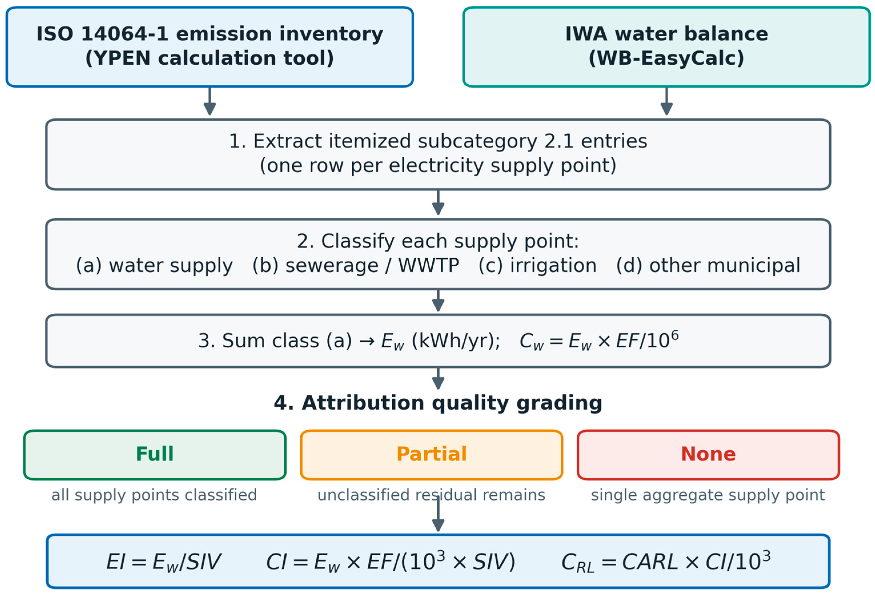
Figure 2.
Composition of the declared emissions of the ten utilities with an inventory, year 2025. (a) Absolute amounts per category; (b) share of fugitive wastewater emissions in the declared total.
Figure 2.
Composition of the declared emissions of the ten utilities with an inventory, year 2025. (a) Absolute amounts per category; (b) share of fugitive wastewater emissions in the declared total.
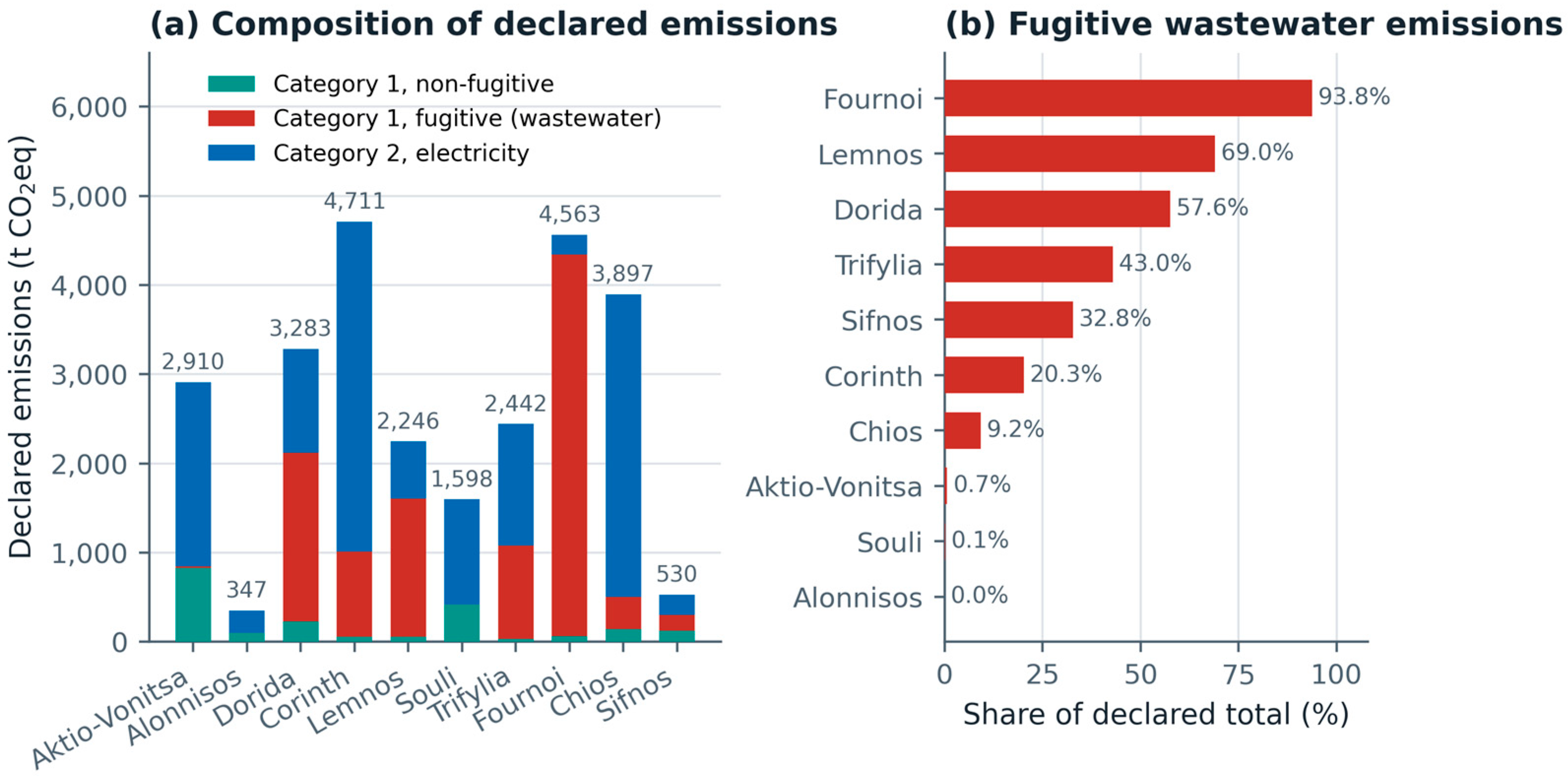
Figure 3.
Electricity attribution quality. (a) Grading per utility and year; (b) water supply share of the utility’s total electricity consumption in 2025. “n/a”: not available due to aggregate metering.
Figure 3.
Electricity attribution quality. (a) Grading per utility and year; (b) water supply share of the utility’s total electricity consumption in 2025. “n/a”: not available due to aggregate metering.
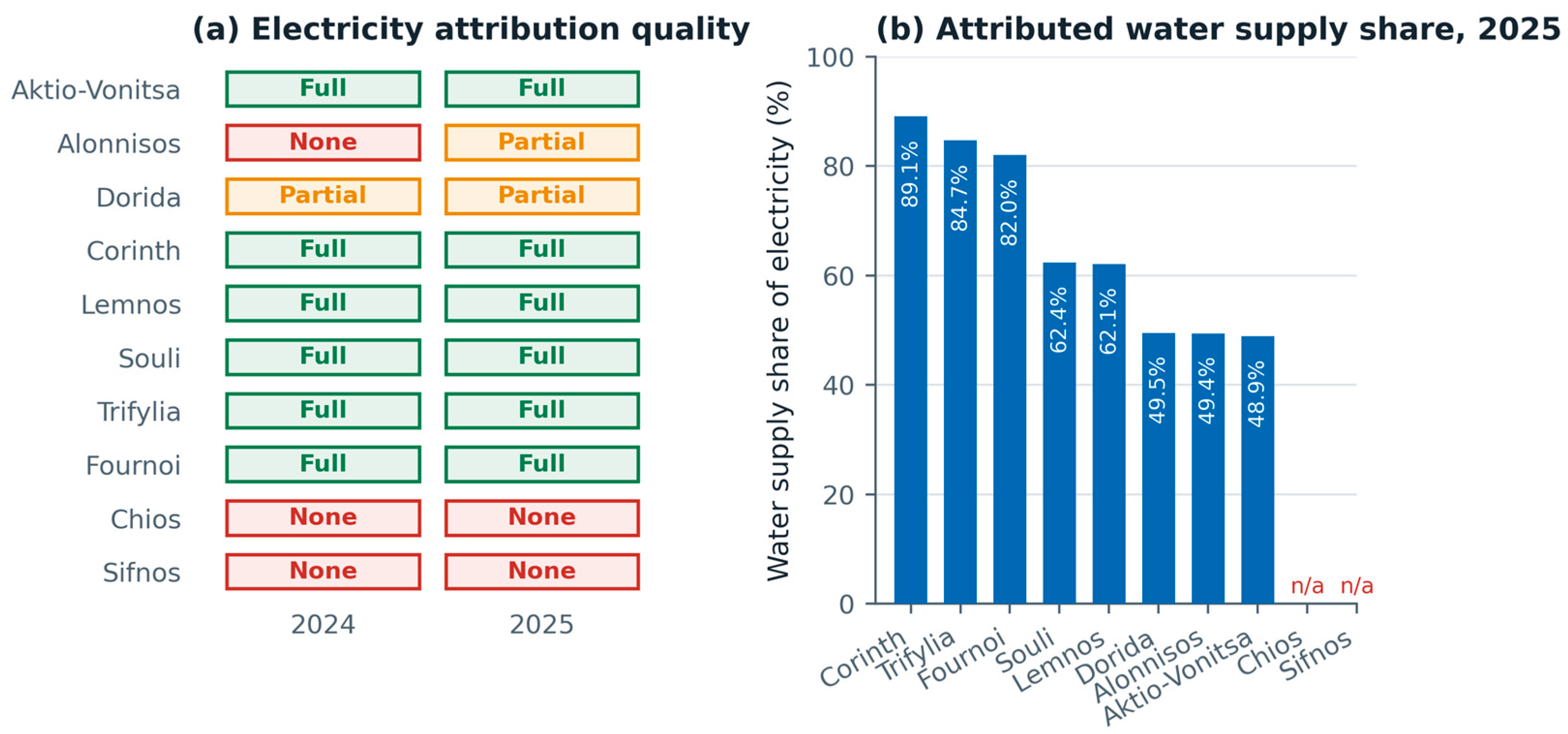
Figure 4.
Distribution of the utility’s total electricity consumption by activity, year 2025. The absolute consumption in GWh is noted above each column.
Figure 4.
Distribution of the utility’s total electricity consumption by activity, year 2025. The absolute consumption in GWh is noted above each column.
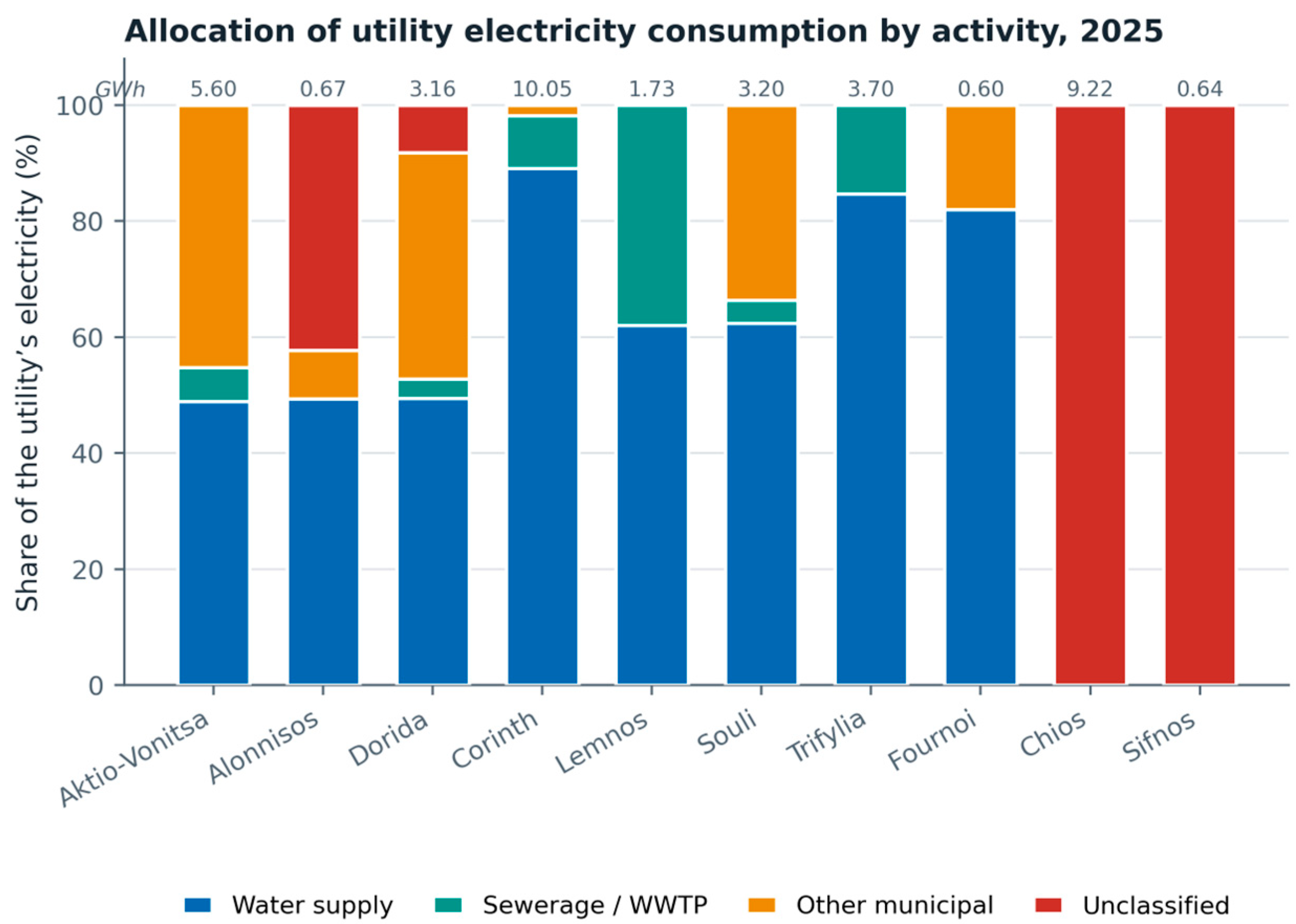
Figure 5.
Attributed system-input carbon intensity (blue) and the organizational-total-to-SIV ratio (red). The number above each pair is the organizational-boundary-mismatch factor r. Logarithmic scale.
Figure 5.
Attributed system-input carbon intensity (blue) and the organizational-total-to-SIV ratio (red). The number above each pair is the organizational-boundary-mismatch factor r. Logarithmic scale.
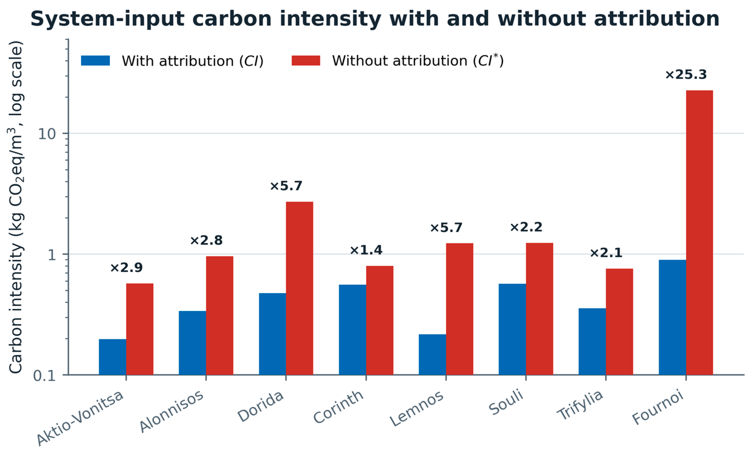
Figure 6.
Composition of the IWA water balance as a share of system input, year 2025, for all eleven utilities. Reported real losses are top-down balance estimates; the internal component split reported by Leros is not used in this three-class presentation.
Figure 6.
Composition of the IWA water balance as a share of system input, year 2025, for all eleven utilities. Reported real losses are top-down balance estimates; the internal component split reported by Leros is not used in this three-class presentation.
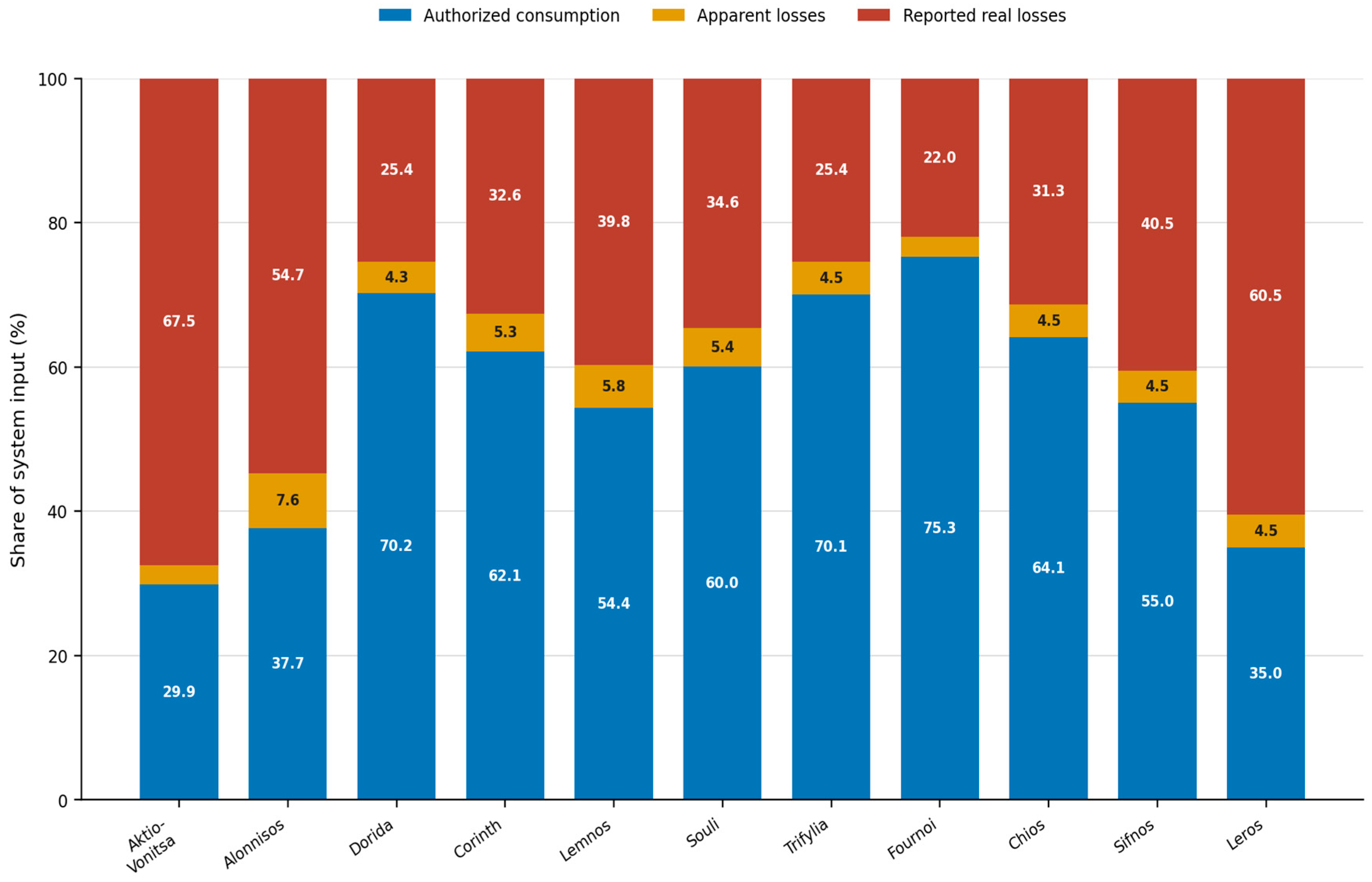
Figure 7.
Non-revenue water and reported real losses as a share of system input, year 2025, for the eleven utilities with a water balance. The dashed line marks the unweighted mean NRW share (46.2%).
Figure 7.
Non-revenue water and reported real losses as a share of system input, year 2025, for the eleven utilities with a water balance. The dashed line marks the unweighted mean NRW share (46.2%).
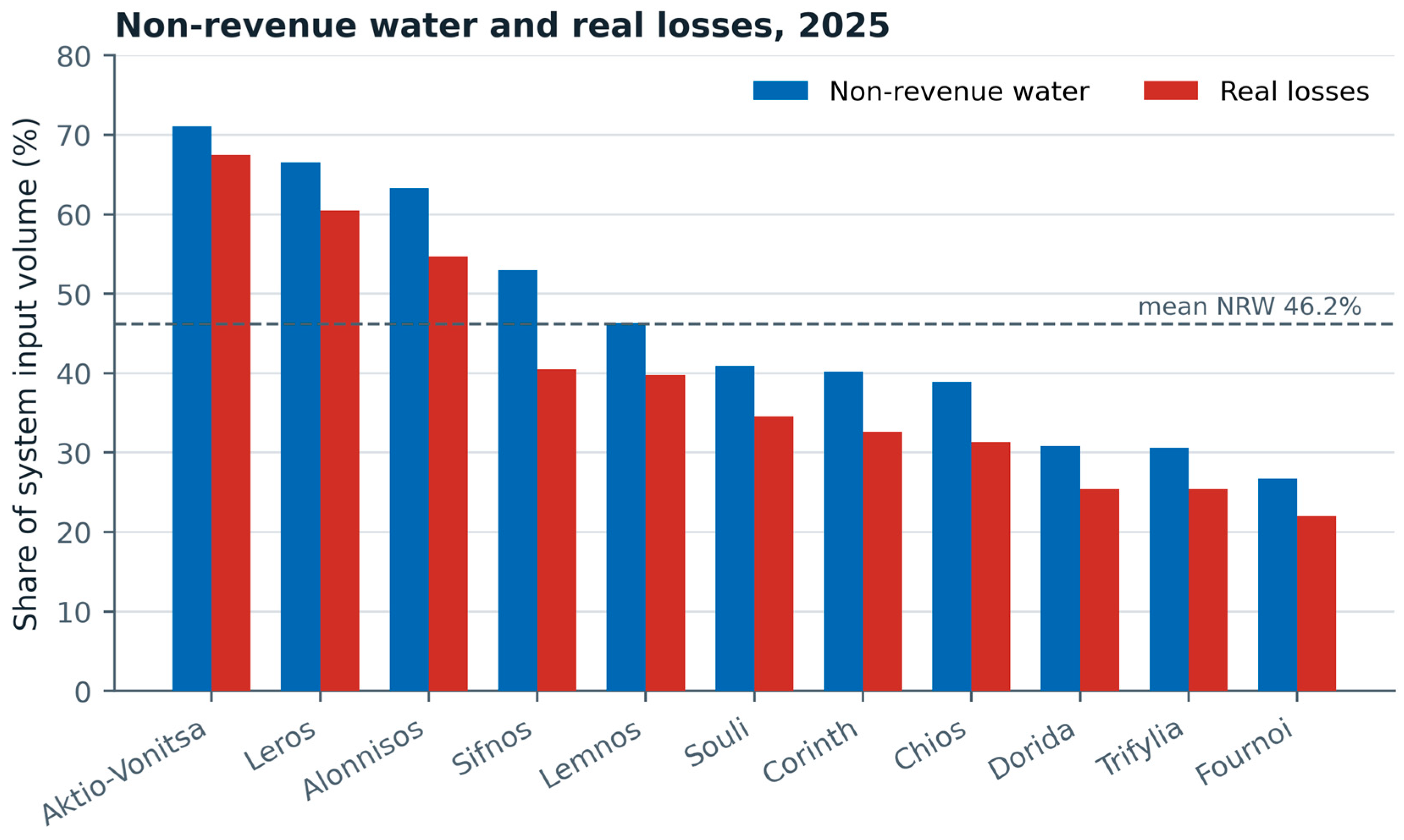
Figure 8.
Energy intensity of water supply per utility and year. The light-blue band reproduces the 0.4–0.9 kWh/m³ distribution range cited in [8,10] for contextual comparison; study boundaries differ.
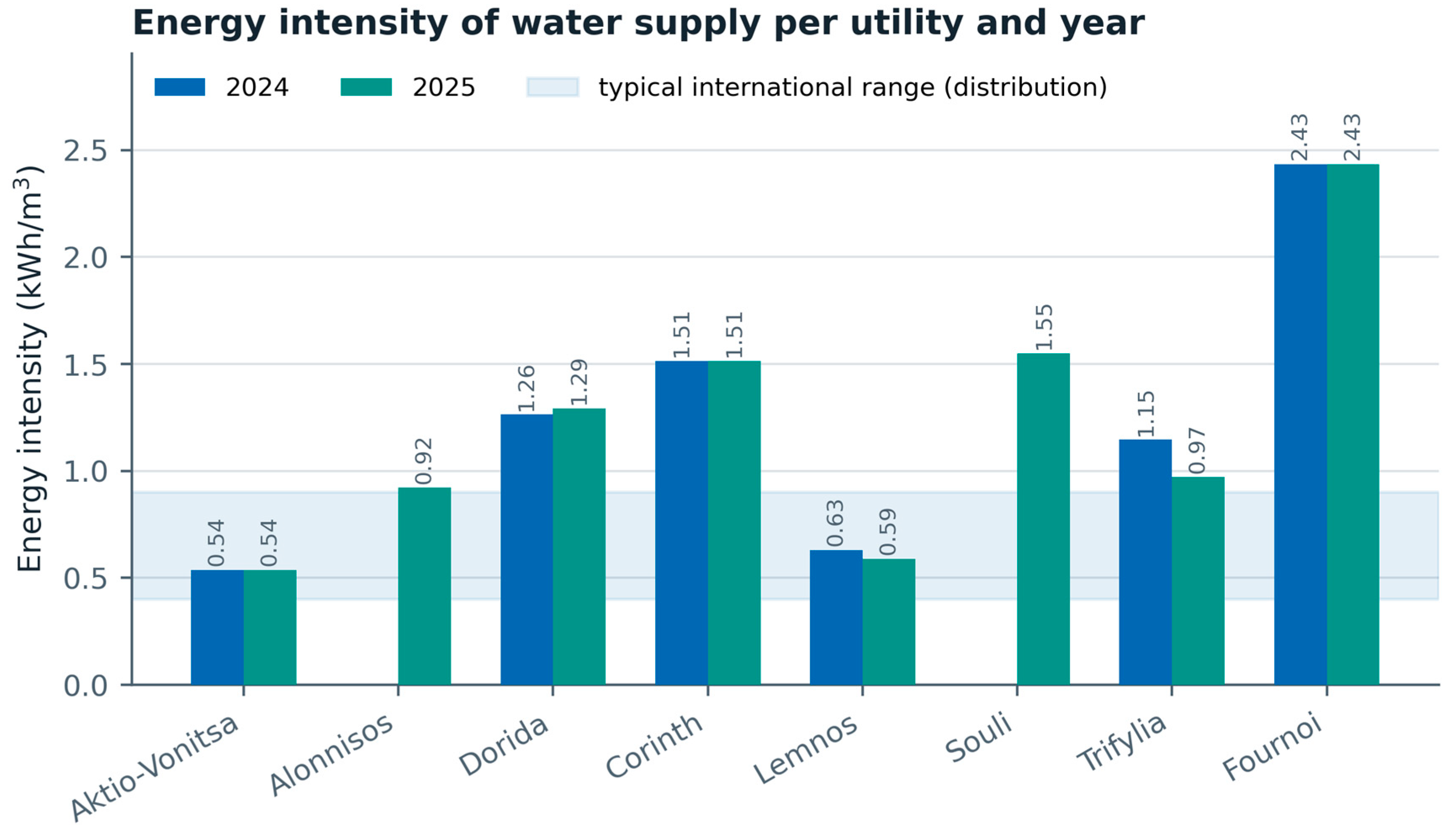
Figure 9.
Operational electricity-related carbon intensity per cubic metre of system input (most recent available year).
Figure 9.
Operational electricity-related carbon intensity per cubic metre of system input (most recent available year).
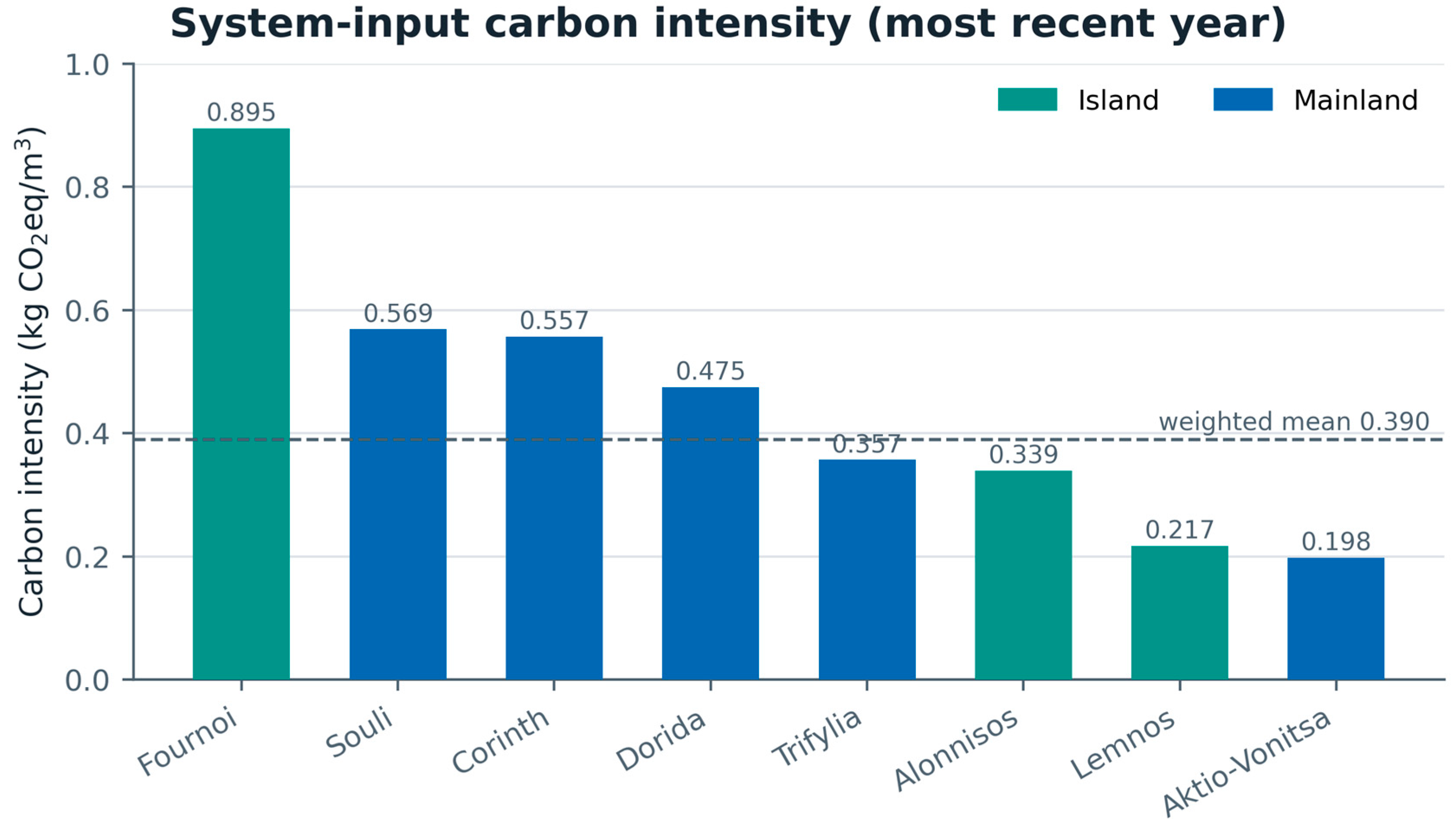
Figure 10.
Energy intensity versus reported real-loss share. Dot size is proportional to system input; semi-transparent dots correspond to 2024. The dashed contours show constant allocated electricity per m³ of system input under average-intensity accounting.
Figure 10.
Energy intensity versus reported real-loss share. Dot size is proportional to system input; semi-transparent dots correspond to 2024. The dashed contours show constant allocated electricity per m³ of system input under average-intensity accounting.
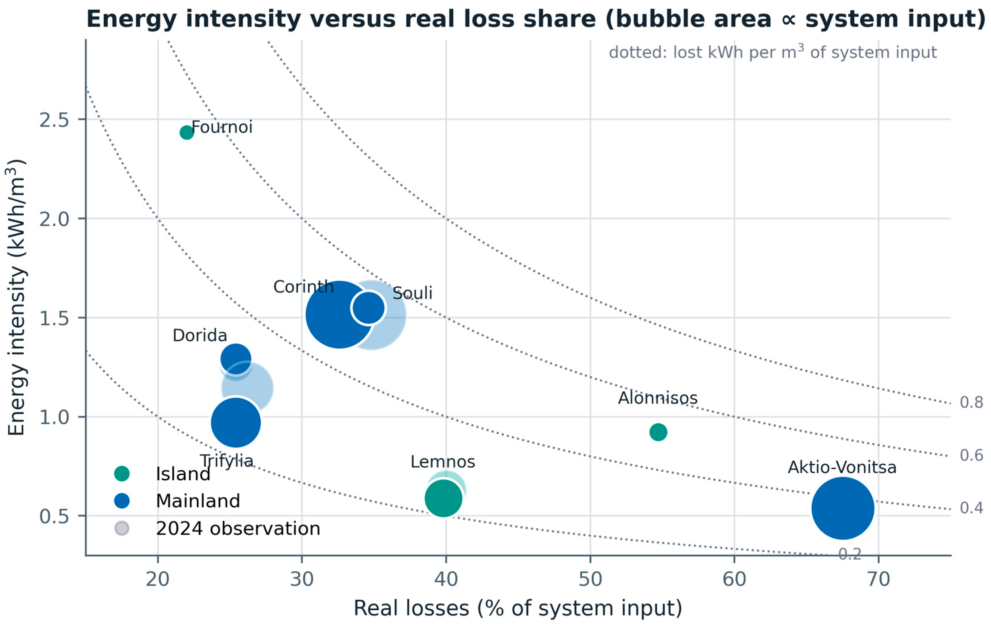
Figure 11.
Emissions allocated to reported real losses. (a) Absolute allocations to real losses and total non-revenue water; (b) allocated share of water-supply electricity emissions.
Figure 11.
Emissions allocated to reported real losses. (a) Absolute allocations to real losses and total non-revenue water; (b) allocated share of water-supply electricity emissions.
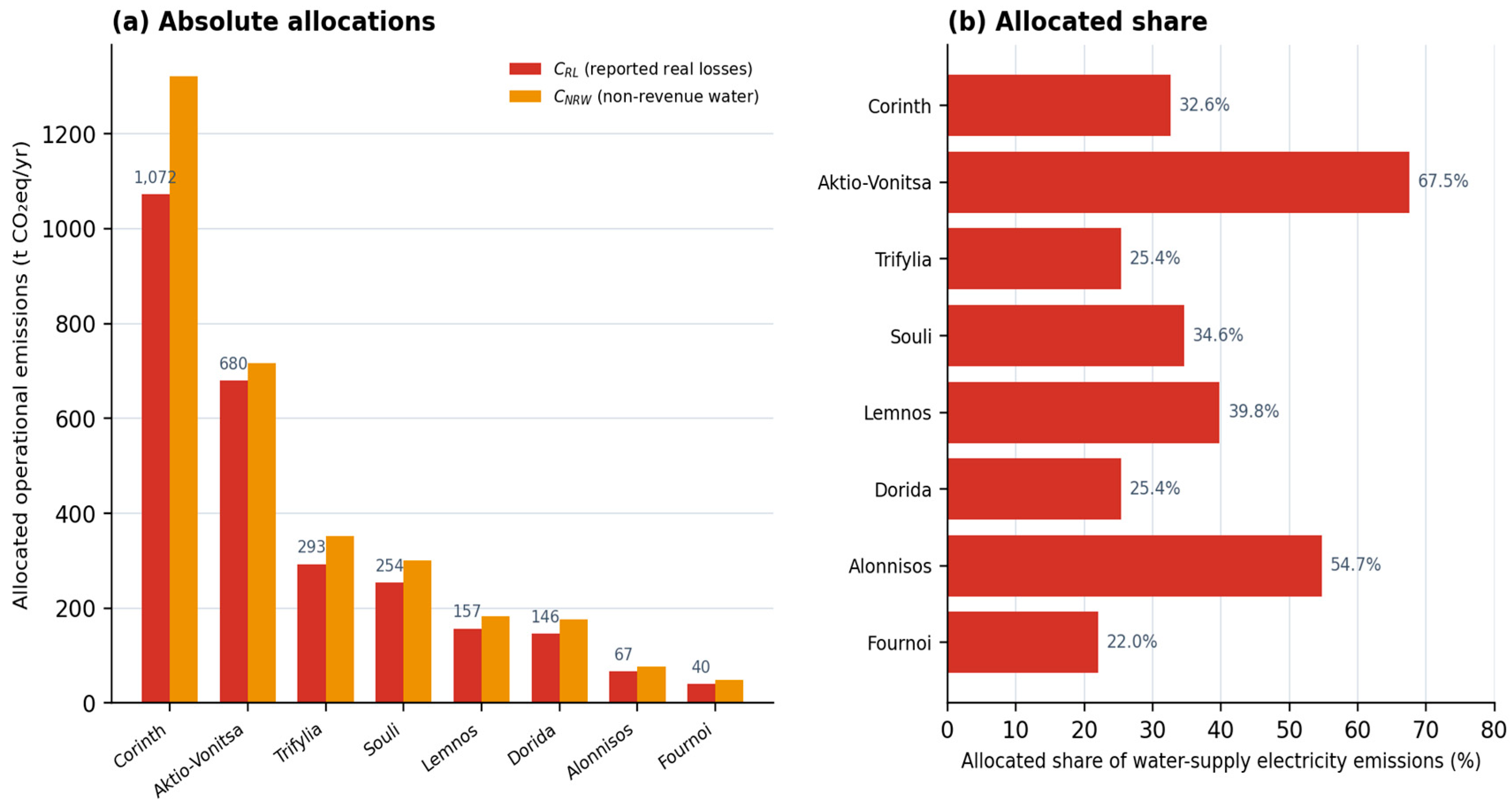
Figure 12.
Proportional average-intensity allocation for the Municipality of Aktio-Vonitsa, year 2025. (a) Submitted water-balance quantities; (b) allocation of average electricity intensity and the emission factor to reported real losses.
Figure 12.
Proportional average-intensity allocation for the Municipality of Aktio-Vonitsa, year 2025. (a) Submitted water-balance quantities; (b) allocation of average electricity intensity and the emission factor to reported real losses.
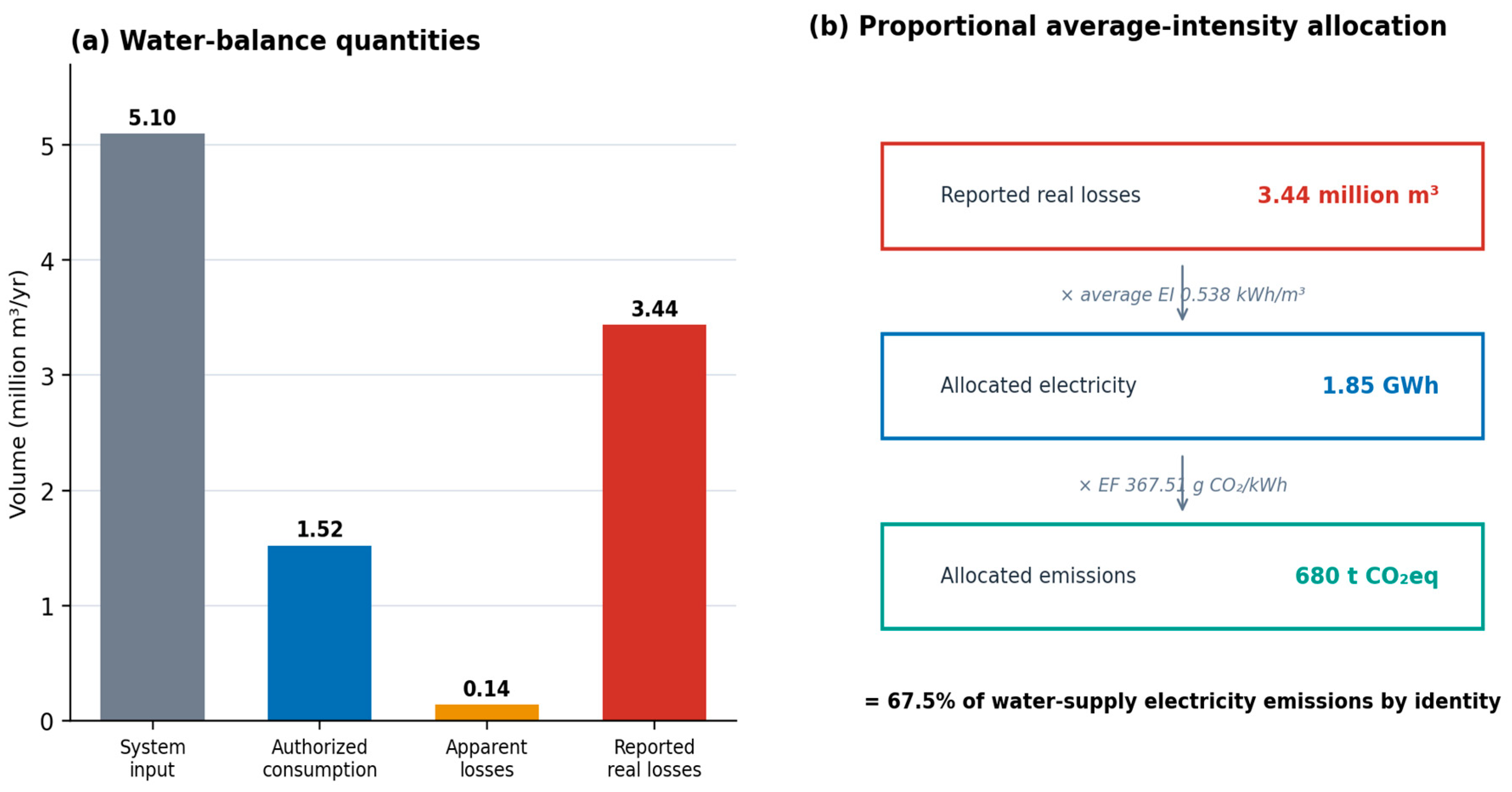
Figure 13.
Contours of operational emissions allocated per m³ of system input as a function of the reported real-loss fraction and average energy intensity. Similar allocations can arise from different system profiles.
Figure 13.
Contours of operational emissions allocated per m³ of system input as a function of the reported real-loss fraction and average energy intensity. Similar allocations can arise from different system profiles.
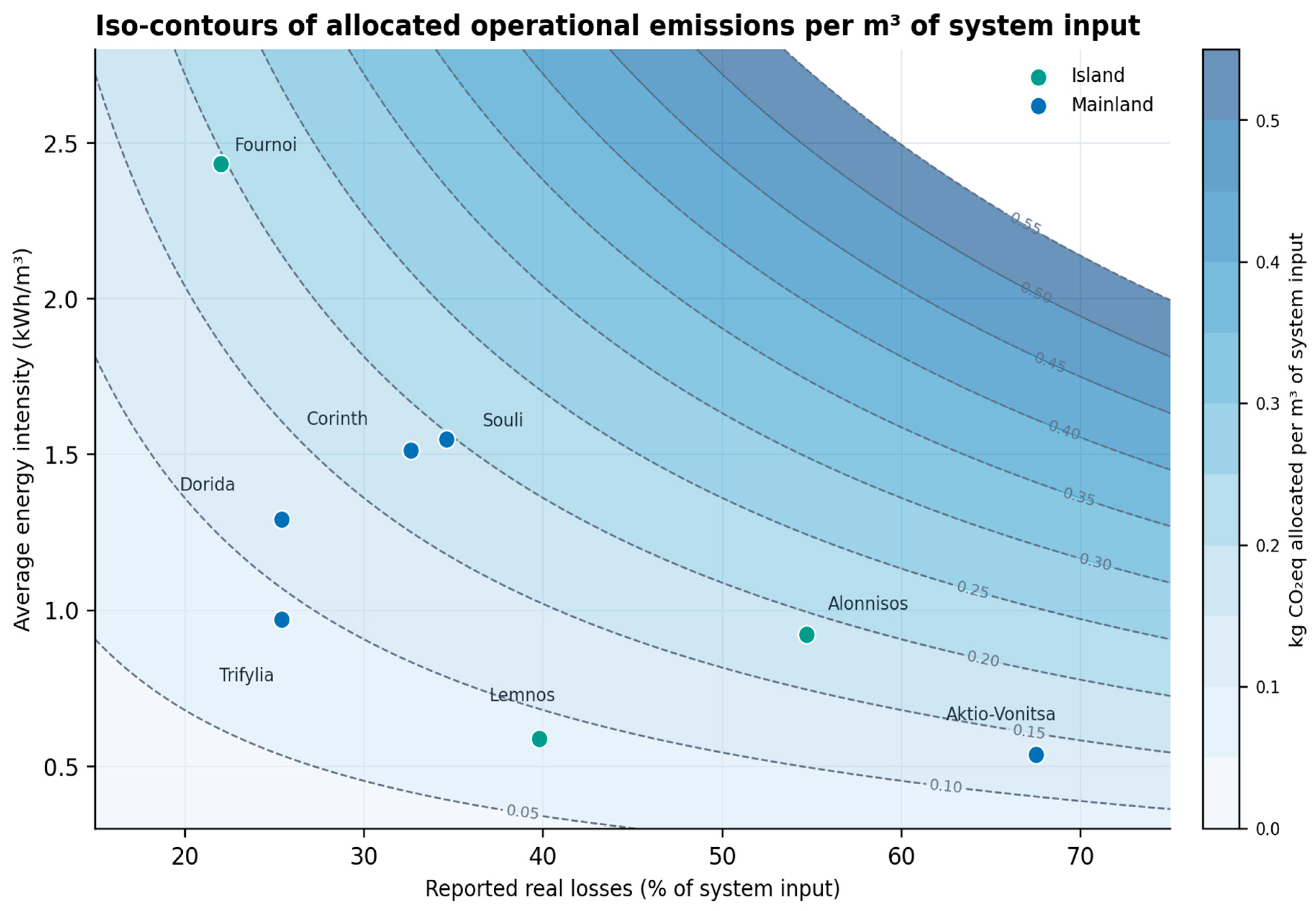
Figure 14.
Conditional marginal abatement cost screening for leakage reduction. (a) Curves as a function of illustrative unit intervention cost, with c = 0.33 €/m³; (b) screening values at I = 0.40 €/m³ and selected external carbon benchmarks.
Figure 14.
Conditional marginal abatement cost screening for leakage reduction. (a) Curves as a function of illustrative unit intervention cost, with c = 0.33 €/m³; (b) screening values at I = 0.40 €/m³ and selected external carbon benchmarks.
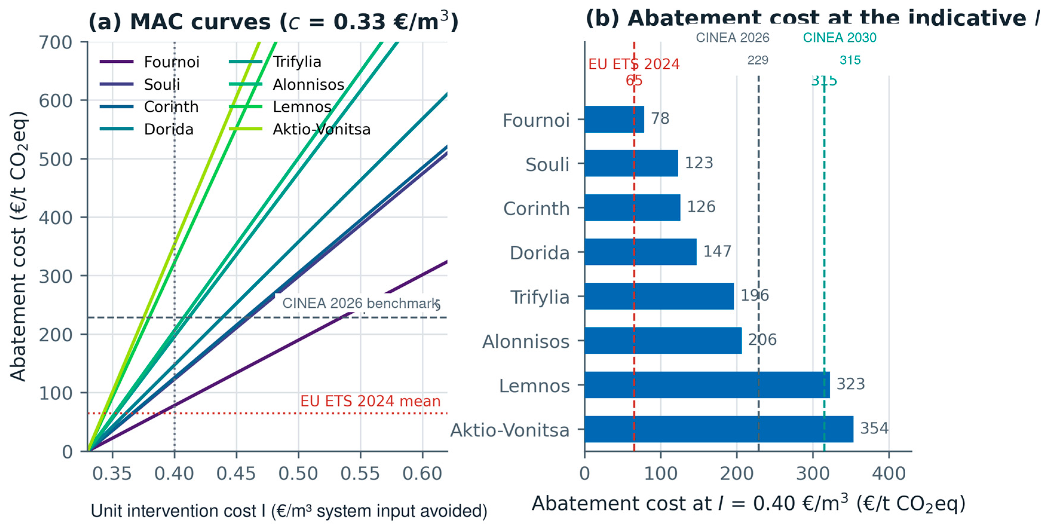
Figure 15.
Scenarios of real loss reduction. (a) Avoided emissions per utility; (b) total benefit and water saved for the eight utilities.
Figure 15.
Scenarios of real loss reduction. (a) Avoided emissions per utility; (b) total benefit and water saved for the eight utilities.
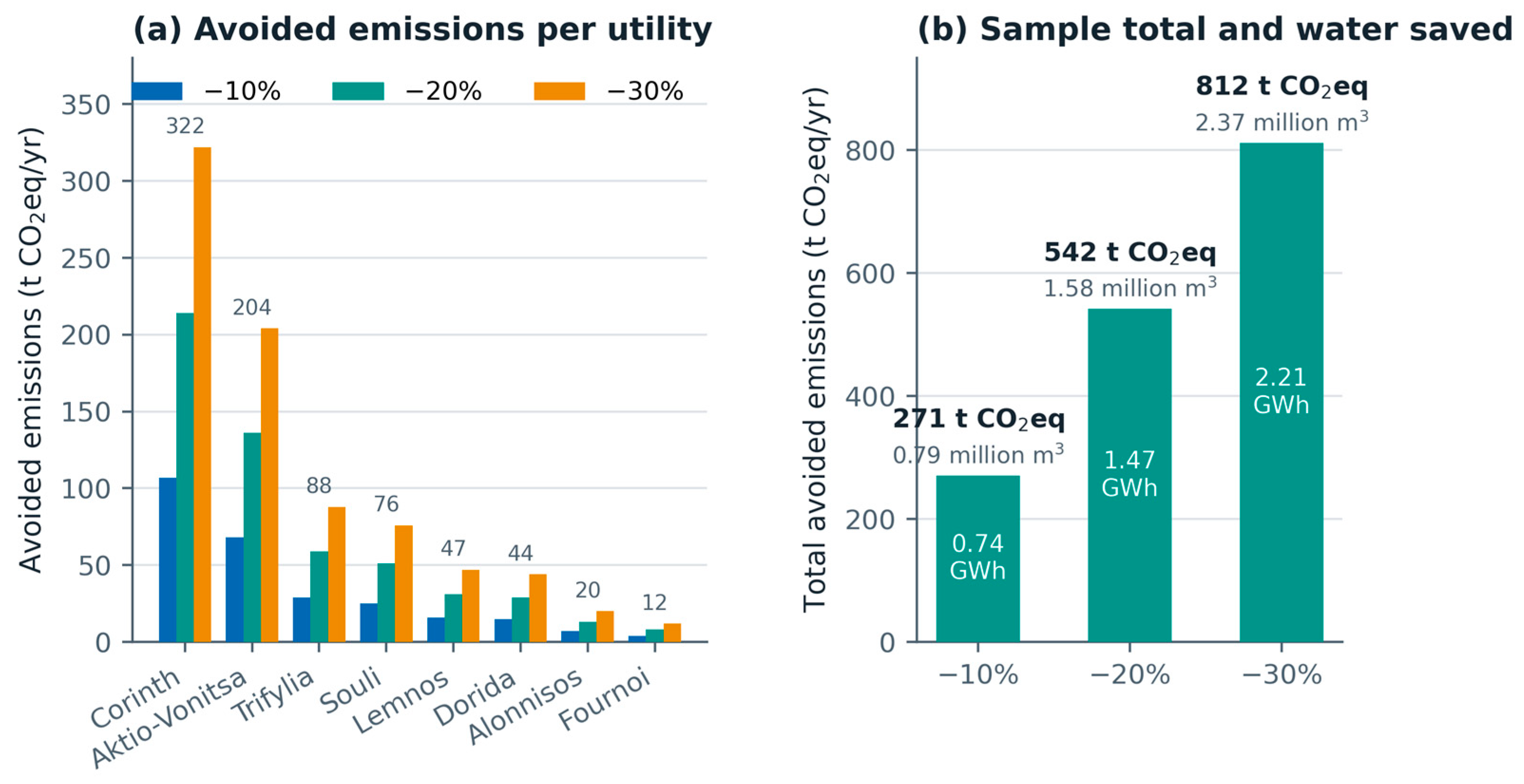
Figure 16.
Scenario of a 20% reduction in real losses: contribution to reducing the utility’s total declared emissions. The absolute amount is noted inside the columns.
Figure 16.
Scenario of a 20% reduction in real losses: contribution to reducing the utility’s total declared emissions. The absolute amount is noted inside the columns.
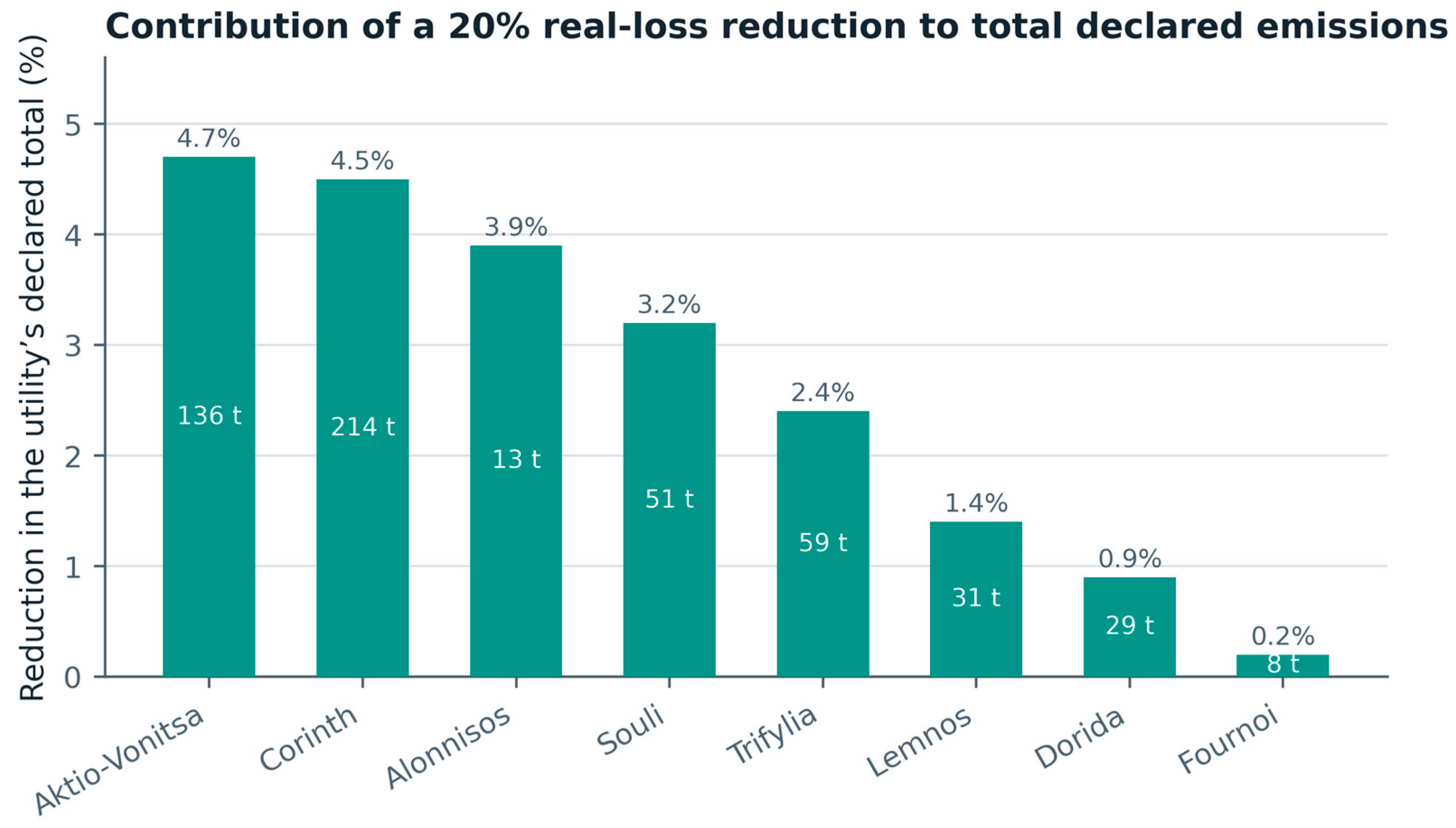
Figure 17.
Comparative panel of normalized indicators per utility for the most recent available year. The colour scale is normalized per column; numbers are actual values. Factor r is the organizational-boundary-mismatch factor. The left strip distinguishes island (green) from mainland (ochre) utilities.
Figure 17.
Comparative panel of normalized indicators per utility for the most recent available year. The colour scale is normalized per column; numbers are actual values. Factor r is the organizational-boundary-mismatch factor. The left strip distinguishes island (green) from mainland (ochre) utilities.
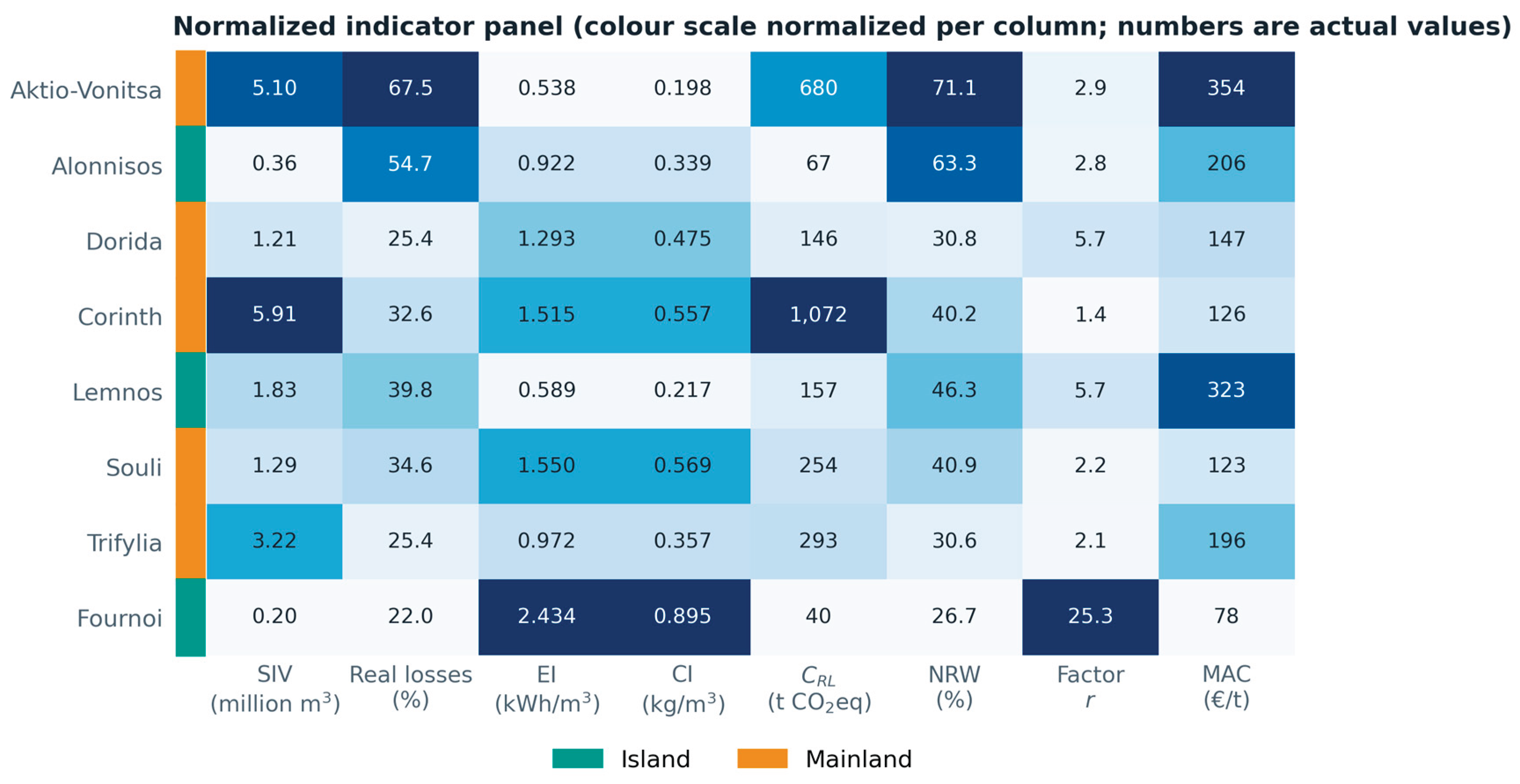
Table 3.
Composition of declared emissions and attribution quality, year 2025.
| Utility | Total (t CO₂eq) |
Cat. 1 (t CO₂eq) |
Fugitive (t CO₂eq) |
Fugitive (%) |
Cat. 2 (t CO₂eq) |
Electricity (GWh) |
Water supply (% of electricity) |
Attribution quality |
|---|---|---|---|---|---|---|---|---|
| Aktio-Vonitsa | 2,910 | 847 | 19 | 0.7 | 2,062 | 5.60 | 48.9 | Full |
| Alonnisos | 347 | 99 | 0 | 0.0 | 248 | 0.67 | 49.4 | Partial |
| Dorida | 3,283 | 2,121 | 1,891 | 57.6 | 1,162 | 3.16 | 49.5 | Partial |
| Corinth | 4,711 | 1,012 | 954 | 20.3 | 3,699 | 10.05 | 89.1 | Full |
| Lemnos | 2,246 | 1,608 | 1,549 | 69.0 | 639 | 1.73 | 62.1 | Full |
| Souli | 1,598 | 420 | 2 | 0.1 | 1,178 | 3.20 | 62.4 | Full |
| Trifylia | 2,442 | 1,080 | 1,049 | 43.0 | 1,362 | 3.70 | 84.7 | Full |
| Fournoi | 4,563 | 4,342 | 4,279 | 93.8 | 221 | 0.60 | 82.0 | Full |
| Chios | 3,897 | 501 | 358 | 9.2 | 3,396 | 9.22 | — | None |
| Sifnos | 530 | 300 | 174 | 32.8 | 230 | 0.64 | — | None |
The “Cat. 1” column includes fugitive emissions. Attribution quality: Full / Partial / None, according to the protocol of Section 2.5.
Table 4.
Attributed system-input carbon intensity and organizational-boundary mismatch.
| Utility | Year | Attributed CI (kg CO₂eq/m³ SIV) |
Organizational ratio CI* |
Boundary-mismatch factor r |
Water supply share of electricity (%) |
Fugitive emissions (% of total) |
|---|---|---|---|---|---|---|
| Aktio-Vonitsa | 2025 | 0.198 | 0.571 | ×2.9 | 48.9 | 0.7 |
| Alonnisos | 2025 | 0.339 | 0.961 | ×2.8 | 49.4 | 0.0 |
| Dorida | 2025 | 0.475 | 2.719 | ×5.7 | 49.5 | 57.6 |
| Corinth | 2025 | 0.557 | 0.798 | ×1.4 | 89.1 | 20.3 |
| Lemnos | 2025 | 0.217 | 1.229 | ×5.7 | 62.1 | 69.0 |
| Souli | 2025 | 0.569 | 1.241 | ×2.2 | 62.4 | 0.1 |
| Trifylia | 2025 | 0.357 | 0.758 | ×2.1 | 84.7 | 43.0 |
| Fournoi | 2025 | 0.895 | 22.632 | ×25.3 | 82.0 | 93.8 |
Table 6.
Energy and carbon intensity and emissions allocated to reported real losses, by utility-year observation.
Table 6.
Energy and carbon intensity and emissions allocated to reported real losses, by utility-year observation.
| Utility | Year | Water supply energy (GWh) |
EI (kWh/m³) |
CI (kg CO₂eq/m³ SIV) |
Water supply emissions (t) |
Lost energy (GWh) |
C_RL (t CO₂eq) |
Share (%) |
C_NRW (t CO₂eq) |
|---|---|---|---|---|---|---|---|---|---|
| Aktio-Vonitsa | 2024 | 2.69 | 0.538 | 0.198 | 989 | 1.82 | 667 | 67.5 | 703 |
| Aktio-Vonitsa | 2025 | 2.74 | 0.538 | 0.198 | 1,007 | 1.85 | 680 | 67.5 | 716 |
| Alonnisos | 2025 | 0.33 | 0.922 | 0.339 | 122 | 0.18 | 67 | 54.7 | 77 |
| Dorida | 2024 | 1.55 | 1.264 | 0.465 | 568 | 0.39 | 145 | 25.4 | 175 |
| Dorida | 2025 | 1.56 | 1.293 | 0.475 | 574 | 0.40 | 146 | 25.4 | 177 |
| Corinth | 2024 | 9.54 | 1.514 | 0.556 | 3,506 | 3.32 | 1,220 | 34.8 | 1,492 |
| Corinth | 2025 | 8.95 | 1.515 | 0.557 | 3,288 | 2.92 | 1,072 | 32.6 | 1,321 |
| Lemnos | 2024 | 1.11 | 0.630 | 0.232 | 408 | 0.44 | 163 | 40.0 | 189 |
| Lemnos | 2025 | 1.08 | 0.589 | 0.217 | 396 | 0.43 | 157 | 39.8 | 183 |
| Souli | 2025 | 2.00 | 1.550 | 0.569 | 733 | 0.69 | 254 | 34.6 | 300 |
| Trifylia | 2024 | 3.93 | 1.146 | 0.421 | 1,445 | 1.03 | 379 | 26.2 | 455 |
| Trifylia | 2025 | 3.13 | 0.972 | 0.357 | 1,151 | 0.80 | 293 | 25.4 | 352 |
| Fournoi | 2024 | 0.49 | 2.434 | 0.895 | 180 | 0.11 | 40 | 22.0 | 48 |
| Fournoi | 2025 | 0.49 | 2.434 | 0.895 | 180 | 0.11 | 40 | 22.0 | 48 |
| 2025 total | 2025 | 20.28 | 1.061 | 0.390 | 7,452 | 7.37 | 2,708 | 36.3 | 3,175 |
EI: energy intensity; CI: operational electricity-related carbon intensity per m³ of SIV; C_RL: emissions allocated to reported real losses; C_NRW: emissions allocated to total non-revenue water. The 2025 aggregate share (36.3%) is ΣC_RL/ΣC_w; ΣCARL/ΣSIV is 41.4%. Fournoi submitted identical values for both years. Totals and weighted indicators use unrounded values and may not equal sums of rounded entries.
Table 7.
Conditional marginal abatement cost screening and intervention-cost thresholds.
| Utility | CI (kg CO₂eq/m³) |
MAC at I = 0.40 €/m³ (€/t CO₂eq) |
I* at 65 €/t (€/m³) |
I* at 229 €/t (€/m³) |
I* at 315 €/t (€/m³) |
Increase in break-even unit cost vs. c (%) |
|---|---|---|---|---|---|---|
| Aktio-Vonitsa | 0.198 | 354 | 0.343 | 0.375 | 0.392 | 13.7 |
| Alonnisos | 0.339 | 206 | 0.352 | 0.408 | 0.437 | 23.5 |
| Dorida | 0.475 | 147 | 0.361 | 0.439 | 0.480 | 33.0 |
| Corinth | 0.557 | 126 | 0.366 | 0.458 | 0.505 | 38.7 |
| Lemnos | 0.217 | 323 | 0.344 | 0.380 | 0.398 | 15.1 |
| Souli | 0.569 | 123 | 0.367 | 0.460 | 0.509 | 39.5 |
| Trifylia | 0.357 | 196 | 0.353 | 0.412 | 0.442 | 24.8 |
| Fournoi | 0.895 | 78 | 0.388 | 0.535 | 0.612 | 62.1 |
Table 1.
Typology of the water service providers in the sample.
| Utility | Type | Location | Relief | Population (ELSTAT 2021) |
Area (km²) |
SIV 2025 (million m³) |
Analytical sample |
|---|---|---|---|---|---|---|---|
| Aktio-Vonitsa | Municipality | Mainland | Lowland/coastal | 14,644 | 660.2 | 5.10 | Yes |
| Alonnisos | Municipality | Island | Island | 3,138 | 129.6 | 0.36 | Yes |
| Dorida | Municipality | Mainland | Mountainous | 12,034 | 998.9 | 1.21 | Yes |
| Corinth | DEYA | Mainland | Lowland/coastal | 55,941 | 611.3 | 5.91 | Yes |
| Lemnos | Municipality | Island | Island | 16,411 | 477.6 | 1.83 | Yes |
| Souli | Municipality | Mainland | Semi-mountainous | 8,759 | 502.8 | 1.29 | Yes |
| Trifylia | DEYA | Mainland | Semi-mountainous | 22,431 | 616.0 | 3.22 | Yes |
| Fournoi | Municipality | Island | Island | 1,343 | 45.2 | 0.20 | Yes |
| Chios | DEYA | Island | Island | 50,361 | 842.3 | 4.23 | No |
| Sifnos | Municipality | Island | Island | 2,777 | 73.9 | 0.55 | No |
| Leros | Municipality | Island | Island | 7,992 | 74.2 | 1.42 | No |
Permanent population refers to the administrative municipality and not necessarily to the served area. The “analytical sample” comprises the utilities for which electricity could be attributed to water supply.
Disclaimer/Publisher’s Note: The statements, opinions and data contained in all publications are solely those of the individual author(s) and contributor(s) and not of MDPI and/or the editor(s). MDPI and/or the editor(s) disclaim responsibility for any injury to people or property resulting from any ideas, methods, instructions or products referred to in the content. |
© 2026 by the authors. Licensee MDPI, Basel, Switzerland. This article is an open access article distributed under the terms and conditions of the Creative Commons Attribution (CC BY) license (http://creativecommons.org/licenses/by/4.0/).
Copyright: This open access article is published under a Creative Commons CC BY 4.0 license, which permit the free download, distribution, and reuse, provided that the author and preprint are cited in any reuse.