

Submitted:
12 August 2026
Posted:
13 August 2026
You are already at the latest version
Abstract
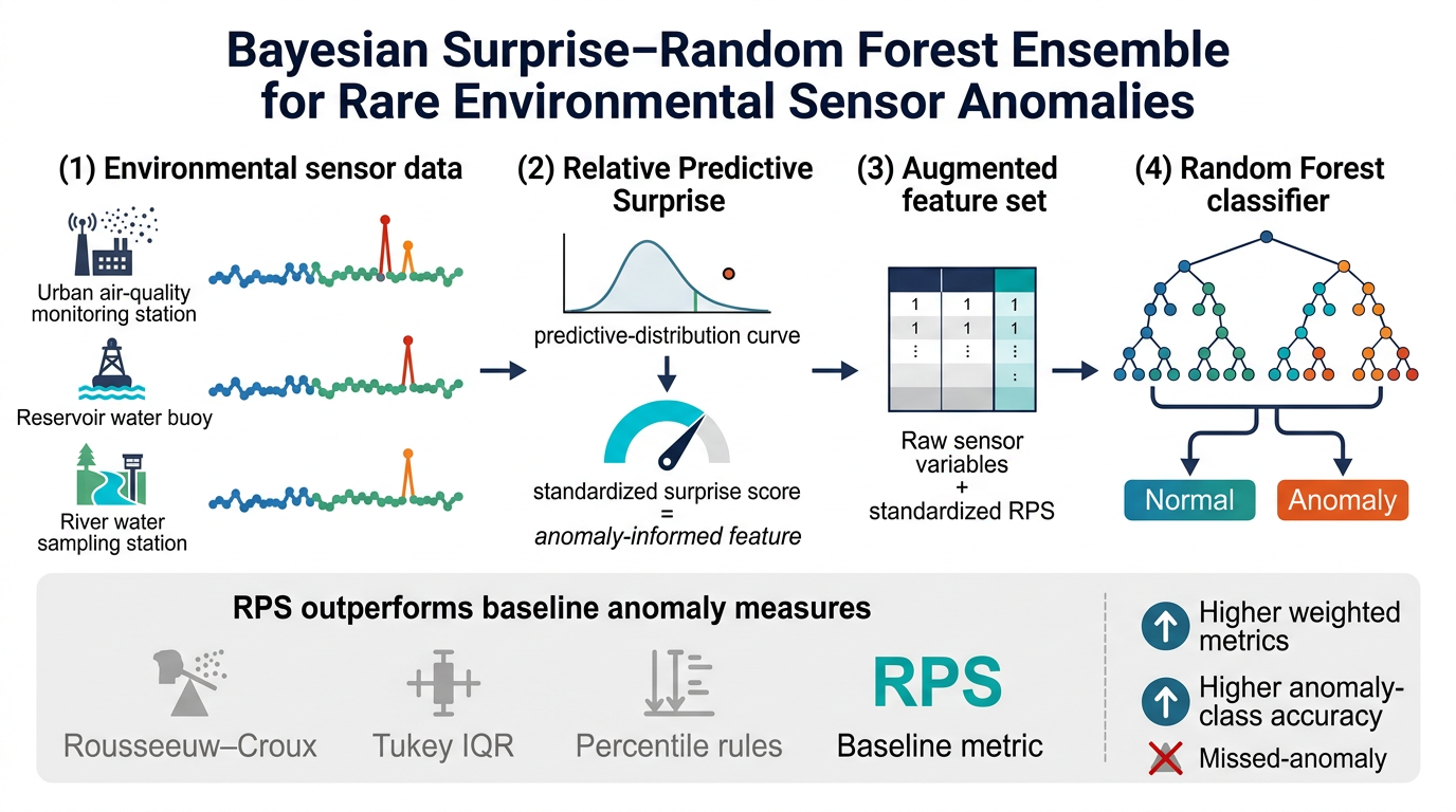
Given the inherent rarity of anomalous readings in environmental sensor data, tree-based models often provide high weighted classification metrics but low anomaly-class recall values, leading to excessive missed anomalies. This study proposes that integrating Bayesian surprise with a random forest classifier can simultaneously enhance weighted classification metrics and class-specific classification accuracy when classifying environmental sensor data. To test this approach, real air-, reservoir-, and river-water quality datasets are used to evaluate the new ensemble method. Bayesian surprise, which is defined using relative predictive surprise, is standardized and serves as an additional anomaly-informed feature. A random forest classifier is employed to classify raw sensor data augmented with the resulting relative predictive surprise values. Empirical experiments indicate that relative predictive surprise is robustly more effective than Rousseeuw–Croux estimators, Tukey interquartile ranges, and percentile-based rules in identifying anomalous sensor measurements. Moreover, augmenting the random forest classifier with relative predictive surprise values improves anomaly-class recall values and weighted classification metrics, indicating fewer missed anomalous sensor measurements. In conclusion, the relative predictive surprise is a computationally simpler and more effective anomaly measure compared to four baseline metrics. This anomaly measure and a random forest classifier emerge as a novel tool for balancing weighted classification metrics and class-specific classification accuracy in classifying environmental sensor data.
Keywords:
Bayesian surprise
; random forest classifier
; heavy-tailed environmental sensor data
; anomaly measure
; data augmentation
1. Introduction
Advances in information technology have enabled the deployment of sensors to monitor environmental phenomena, such as air and reservoir water quality. For example, the Taiwanese government has installed environmental sensors to measure total phosphorus, chlorophyll a, and transparency to warn of critical river water quality. The government shares historical sensor measurements with residents through websites. Flagging anomalous sensor readings is governed by specific rules published on these websites.
Nevertheless, recent severe climatic changes or extreme events may cause environmental sensor data to undergo distribution shifts. New observations and old sensor measurements follow different probability distributions. Thus, it is difficult to apply a single probability distribution to model the sensor data and flag anomalous sensor measurements. It may therefore be necessary to recalibrate frequently existing rules to accommodate new anomalies.
Machine learning algorithms can help mitigate the burden of frequent recalibration of existing rules. In practice, training tree-based models for accurately processing large volumes of data has become feasible and computationally efficient. Such models may be trained to separate normal and anomalous sensor data, and human experts next inspect the resulting predictions to decide whether to accept or override the detected anomalies. However, a challenge may be encountered in implementing such an idea. Since anomalous data are naturally infrequent, tree-based models often fail to achieve balanced classification performance between normal and anomalous sensor data [1,2]. They may output high weighted classification metrics, but anomaly-class recall values remain low, implying that excessive false negatives have been generated.
This study proposes that integrating Bayesian surprise (e.g., [3]), defined using relative predictive surprise (), with a random forest classifier may balance weighted classification metrics and the class-specific classification accuracy. values are first computed, standardized, and then added as anomaly-informed features for real air quality, reservoir water quality, and river water quality datasets. Before augmenting with these values as new features, the resulting predictive surprise values are compared to the Rousseeuw–Croux estimators [4], the Tukey interquartile range [5], and a simple percentile-based rule to ensure that they correctly flag anomalies on complementary cumulative probability curves. A random forest classifier is next employed to classify the augmented datasets. Based on empirical results, this study investigates whether the corresponding weighted classification metrics and the class-specific classification accuracy are simultaneously improved after adding the values as new features.
This study anticipates that this research will fill three research gaps to make the corresponding contributions:
- The first research gap is the lack of a computationally simple anomaly measure for environmental sensor data, which usually exhibit heavy tails. Calculating the requires fewer steps than the computation of Rousseeuw–Croux estimators.
- The second research gap concerns the performance of tree-based models in classifying environmental sensor data. Since anomalous environmental sensor measurements are naturally infrequent, tree-based models tend to focus on improving weighted classification metrics and may cease to optimize the classification accuracy of anomalous classes once the weighted accuracy is maximized [1,2]. This study aims to balance weighted classification metrics and the class-specific classification accuracy by aggregating values as new anomaly-informed features.
- The third research gap concerns the robustness of anomaly thresholds for heavy-tailed sensor data. When existing anomaly measures (for example, Rousseeuw–Croux estimators and percentile rules) are applied to different heavy-tailed distributions, the thresholds for separating normal and abnormal sensor readings may need to be re-tuned for more accurate separation. In contrast, relative predictive surprise is robust to different tail behaviors. This study adopts a fixed anomaly-detection criterion based on across all heavy-tailed environmental sensor datasets.
- The final contribution of this study is enhanced explainability. Without an anomaly measure, a tree-based model is like a ’black box’ in classifying normal and anomalous sensor data. It provides only limited explainability for its classification results. This study integrates a tree-based model with values as anomaly-informed features to provide distribution-level information about how unexpected each sensor reading is, thereby improving the explainability of the resulting classifier.
The remainder of this article is organized into five sections. Section 2 presents a literature review relevant to this study. Section 3 elucidates Bayesian surprise and provides a brief review of the random forest classifier. Section 4 reports experimental results that test the combination of relative predictive surprise values and the random forest classifier on three real datasets of air quality, reservoir water quality, and river water quality. Based on these results, Section 5 offers a discussion. Section 6 presents the conclusions of this study.
2. Literature Review
Because environmental sensor data commonly exhibit heavy-tailed behaviors, the first part of this literature review focuses on prior studies that proposed anomaly measures for heavy-tailed data. The second part reviews published studies on data augmentation methods for heavy-tailed data, since this study calculates values from real environmental sensor datasets and uses them as additional anomaly-informed features.
2.1. Anomaly Measure for Heavy-Tailed Data
A brief review of the literature on anomaly measures for heavy-tailed data identifies two important research gaps. First, a reliable threshold for distinguishing normal observations from anomalous ones has not yet been established. If a reliable threshold is unavailable, augmenting with anomaly-informed features provided based this threshold may not be confidential. Second, the computation of existing anomaly measures often remains unnecessarily complex. In published studies, anomaly measures for heavy-tailed data have generally been grouped into three main categories:
The first approach is based on extreme value theory and tail modeling [7,8,9,10,11]. Rather than modeling the entire heavy-tailed distribution to distinguish normal observations from anomalies, this approach focuses on the tail behavior and fits the tail using a specific probability distribution, such as the generalized Pareto distribution. Anomalies are then identified on the basis of the fitted tail model. In general, the choice of tail model depends on the heaviness and shape of the tail. Representative studies suggest that the Hill estimator [7] is one of the most widely used methods for characterizing tail heaviness. To address finite-sample issues, a previous study [8] proposed a trimmed version of the Hill estimator. Building on this idea, Bhattacharya et al. [9] developed an automatic, data-driven procedure for flagging observations that deviate from the central and intermediate structure of the data. Verardi and Croux [10] extended Tukey’s interquartile range method [5] by incorporating the medcouple to account for skewness in both univariate and multivariate settings, thereby producing an adjusted boxplot for outlier detection. Li et al. [11] estimated sample skewness and constructed empirical cumulative distribution functions to identify tail regions, which were then used to aggregate tail probabilities and define an outlier score.
The second approach comprises probability- and kernel-based methods for modeling heavy-tailed distributions. In this approach, researchers first derive parametric or nonparametric expressions to describe a heavy-tailed distribution, and then identify anomalies based on the resulting probability models. Horváth et al. [12] employed copula functions to estimate the joint distribution of a multivariate heavy-tailed random vector and constructed an anomaly score from the resulting copula-based estimation. A copula enables separate modeling of the marginal distributions and their dependence structure, capturing only the dependency among variables in a multivariate distribution. Bourigault and Mandic [13] combined generalized hyperbolic processes with kernel density estimation and one-class support vector machines to develop anomaly detection frameworks, where the anomaly score is defined using the fitted probability density function. Tortora et al. [14] proposed a model-based clustering approach based on mixtures of multiple scaled contaminated normal distributions to effectively accommodate skewness, heavy tails, or their combination in the classification of heavy-tailed data. This framework allows (1) flexible cluster shapes in terms of skewness and kurtosis and (2) component-wise and directional outlier detection.
The third approach focuses on deep learning models for representing complex, high-dimensional heavy-tailed data distributions. However, most of these models were originally designed for detecting anomalous images. A key distinguishing feature among the models lies in their learning mechanisms. For example, Zenati et al. [15] investigated generative adversarial networks and proposed adversarially learned anomaly detection, in which images with large reconstruction errors are identified as anomalous. Dionelis [16] also explored generative adversarial networks and adopted a similar reconstruction-based criterion for anomaly detection; however, their learning objective is to reconstruct the tail region of a heavy-tailed data distribution. Yang et al. [17] developed a transformer-based reconstruction module for image anomaly detection.
2.2. Data Augmentation Methods for Heavy-Tailed Data
This study proposes that augmenting heavy-tailed data with values may improve the accuracy of classifying these data using a random forest classifier. A concise review of prior studies on data augmentation methods for heavy-tailed data reveals two research gaps. First, existing data augmentation methods for heavy-tailed data are largely restricted to specific application domains (for example, image classification), and their implementation can be inefficient because they typically require tuning many hyperparameters. For instance, a recent study [6] developed a distance-based scheme to enhance the performance of a random forest classifier; however, training this classifier must be performed twice to tune certain hyperparameters.
Other relevant studies in image classification are also available. Ma et al. [18] observed a substantial imbalance between the numbers of normal and abnormal images in an image classification problem. To address this issue, they proposed a four-phase training scheme for a conventional neural network. The second phase of this scheme incorporates a feature-uncertainty representation based on a Gaussian distribution, which provides probabilistic features of the decision boundary separating normal and abnormal images. Introducing this probabilistic feature improves the image classification performance of a convolutional neural network.
Song et al. [19] also investigated image classification problems. They developed a contrastive visual–language model that consists of visual and semantic components. The visual components were created using images, whereas the semantic features are generated using the text sequences associated with the images. Experimental results demonstrated that the proposed contrastive visual–language model improves the F1 scores for classifying normal and abnormal images.
Delaigle and Hall [20] investigated the effect of heavy tails on cardiomyopathy microarray data and Affymetrix spike-in data. They calculated statistical features to conduct their analysis. The purpose of this calculation is to recover influential genes that would otherwise be incorrectly discarded due to the presence of outliers.
3. Methods
Suppose represent a collection of N environmental sensor measurements. These may be acquired asynchronously. Each is a an n-dimensional tuple, . Each may be either normal or anomalous.
3.1. Bayesian Surprise
Suppose a null hypothesis states that the collected sensor measurements follow a specific probability distribution, such as the Student’s t distribution. A new observation may be a newly observed value for the j-th sensor variable. It may be an outlier of if its resulting p value is below a predetermined significance level (e.g., ). This outlier is a potential anomaly. The p-value is calculated by [3]
where and , is the mean of referenced sensor measurements, s is their standard deviation and Pr denotes the probability. This Pr is equal to in which denotes the number of observations equals to t. However, the distribution of may exhibit heavy tails. The p value-based anomaly detection may therefore yield excessive false positives. To address this issue, scholars proposed alternative approaches (e.g., [21]) that better characterize the rarity of an observation with respect to the reference measurements . In this study, considering that reference measurements follow an unknown distribution, the Bayesian surprise, defined through the [3], is adopted to assess whether a is rare. For discrete sensor measurements, the is defined by [3,21,22]:
where sup is the supremum, the subscript denotes the maximum, , and . The theoretical foundation of Equation (2) is related to the Kullback-Leibler divergence [23]. Unlike conventional approaches that seek observations inconsistent with a specific probability distribution, Equation (2) is used in this study to identify sensor readings that are relatively rare in the reference sensor data.
The surprise index can be used to determine whether is anomalous [21,22]. We can derive:
where represents the surprise index. Equation (3) indicates that the maximum of the is equal to the reciprocal of the . This relationship may serve as an important basis for determining the threshold at which an value implies an anomaly. Table 1[24] presents the referenced rules for flagging anomalies based on and [24].
3.2. Random Forest Classifier
Suppose represent the N tuples consisting of raw sensor data and their vslues in which and and Y is the class label. To avoid data leakage and possible confusion with the training-test split used in random forest classification, it must be emphasized that the value of a new observation (or ) is computed based on the N raw reference observations .
A random forest is a tree-based ensemble learning algorithm in which each tree is constructed using a random subset of the available information [25]. In classification tasks, it learns a prediction function from the training observations to predict the class label Y. The learning objective is defined through a loss function , which quantifies the mismatch between the predicted and actual labels. For classification under the zero-one loss criterion, the optimal prediction function is obtained by minimizing the expected loss where the expectation is taken over the joint distribution of and Y. A commonly used loss function is [26]:
where I is the indicator function. If is the set containing all possible Y values, minimizing the for the zero-one loss results in
In ensemble learning, the prediction function f is constructed from a collection of base learners in which denotes the random variables used to build the k-th learner. These random variables are assumed to be independent, and the resulting base learners are aggregated to form the final prediction function f:
The learners build the tree classifier by recursively splitting the training data data into a splitting criterion that measures the purity of a leaf node. In this study, the index is chosen as the splitting criterion. It is defined as
where C is the number of classes and denotes the proportion of observations belonging to class i in the node. Data partitioning based on Equation (7) is carried out recursively until a stopping criterion is satisfied. For classification of a new observation, the observation is propagated through each tree in the forest until it reaches a terminal node. Unlike a single decision tree model, random forest does not require pruning during tree growth. The absence of pruning simplifies model construction and is one of the practical advantages of random forest.
Algorithm 1 [26] presents the procedure for constructing a random forest classifier. First, bootstrap samples are generated from the observations data. This step returns each bootstrap sample to the by sampling with replacement. Each bootstrap sample is then used to grow a classification tree until a stopping criterion is met. During this process, the sample is recursively split to determine the best partition at each node.
| Algorithm 1 Random forest classifier [26] |
|
In addition to the index, several hyperparameters must be specified when implementing a random forest classifier, including:
- Maximum depth of the tree;
- Number of trees in the forest;
- Minimum number of samples required to split an internal node; and
- Minimum number of samples required to be at a leaf node.
Section 4.4 further examines the effects of these four hyperparameters on the classification accuracy of a random forest classifier with and without the inclusion of values as anomaly-informed features.
4. Applications
To improve the quality of life, the Taiwanese government has deployed environmental sensors to monitor environmental conditions, including air quality, reservoir water quality, and river water quality. It has also constructed websites to share historical sensor measurements. This study uses three real datasets collected from these websites to evaluate the performance of the random forest classifier and .
4.1. Air Quality
The first real dataset contains 24,007 records of SO2, CO, NO2, PM2.5, and air quality index (AQI) measurements [27]. These measurements were collected daily in 2024 from 60 monitoring stations across Taiwan. The units of SO2 and NO2 are ppb, whereas that of CO is ppm. The unit of PM2.5 is . Figure 1 depicts the distributions of SO2, CO, NO2, PM2.5, and AQI. Table 2 presents their summary statistics, where denotes the Tukey interquartile range, and represents the trimmed Hill index [8].
As mentioned earlier, the trimmed Hill index [8] was used to characterize the heaviness of a tail. For the j-th sensor measurement, suppose denote the ordered sensor data. The trimmed Hill index is defined as [7,8]
where , and denotes the number of the largest extremes trimmed from the estimation, with . Based on the published article [8], Table 3 presents our interpretation of the resulting values. These values are used as practical reference thresholds rather than universal decision rules. In practice, and can be computed using standard spreadsheet software.
As expected, Figure 1 and Table 2 suggest that the distributions of SO2, CO, NO2, PM2.5, and AQI exhibit substantial upper-tail heaviness. Evidence includes the large kurtosis values and high values in Table 2, as well as the pronounced upper-tail spread shown in Figure 1. Under such distributional characteristics, applying the standard Z-score to anomaly detection may yield incorrect detections. Extreme can inflate their mean and standard deviation, thereby masking potential anomalies.
Furthermore, Equation (9) presents the Pearson correlations among SO2, CO, NO2, and PM2.5. In particular, CO and NO2 exhibit a strong positive correlation. Equation (9) suggests that these two pollutants may share common emission sources, potentially related to fossil-fuel combustion.
Next, this study combines a log-log plot and dumbbell plots to compare the ranges of anomalies identified by the and four baseline metrics. Since the values reported in Table 2 suggest substantial upper-tail heaviness, the Tukey interquartile range (), the Rousseeuw-Croux estimators and , and a simple percentile-based rule are adopted as baselines. According to the , a sensor measurement is considered anomalous if it satisfies
in which and are the first and third quartiles; respectively. Meanwhile, Rousseeuw-Croux estimators and [4] are defined as
where, for each k, and . Here, is the absolute value, and denotes the L-th order statistic obtained by sorting all pairwise distances for in an ascending order and selecting the L-th element. Moreover, where floor denotes the floor function, ! represents the factorial, , and .
A log-log plot is employed to separate the regions associated with normal and anomalous observations on the complementary cumulative probability curve. In this plot, anomalous observations tend to occupy an approximately linear segment. As shown in Figure 2(a)-Figure 2(d), the slope between adjacent black points is calculated to detect this approximately linear segment. This segment is shaded in gray in Figure 2(a)-Figure 2(d). The 90th percentile is further marked as a reference threshold to verify the placement of the gray region. Blue, orange, red, and green dumbbells in Figure 2(a)-Figure 2(d) represent the anomaly ranges identified by , , , and , respectively, and the legend in each panel lists the corresponding criteria.
Figure 2(a)-Figure 2(d) demonstrate that Equation (2) is more effective than Equations (10)-(12) in detecting anomalous pollutant concentrations. In Figure 2(a)-Figure 2(c), the left boundaries of the gray regions closely align with the 90th percentiles, while in Figure 2(d) the discrepancy between the left boundary and the 90th percentile is negligible. These results indicate that the gray regions provide sufficiently accurate estimates of the ranges occupied by anomalous pollutant concentrations in all four plots. The blue dumbbells are consistently located close to the gray regions, supporting the effectiveness of Equation (2). In contrast, although the orange dumbbell in Figure 2(a) is also close to the gray region, the orange dumbbells in Figure 2(b)-Figure 2(d) are shorter than the widths of the corresponding gray regions, suggesting that Equation (10) yields an excessive number of false negatives. Moreover, lowering the thresholds from and to and could improve the agreement between the red and green dumbbells and the gray regions. This observation suggests that the original thresholds, and may be overly conservative for anomaly detection.
Next, this study applies a random forest classifier to classify the collected air quality data. Before training the random forest classifier, standardizing the values of these air quality data is implemented; thus, they can be incorporated as anomaly-informed features. For the SO2 concentration, its standardized is calculated by
where the overline denotes the standarization, the represents the value derived from the SO2 concentration, and are its median and ; respectively. Applying the same procedures yields , , and .
In Taiwan, the AQI is used to indicate whether air quality may be unhealthy. Based on the AQI regulation [27], the official six-category AQI is consolidated into three health-oriented categories. The class of good to acceptable contains the official categories of good and ordinary air quality are combined into a class of good to acceptable, whereas the class of unhealthy is composed of the categories of unhealthy, very healthy, and harmful. Accordingly, this study defines the class label Y in the form as
where Equation (14) yields 22,534 instances for , 1,367 instances for , and 106 instances for , indicating substantial class imbalance.
The random forest classifier is subsequently trained on the collected air quality data enriched with standardized -based features. Within this framework, the standardized variables do not determine or alter the class labels Y. Instead, they function as auxiliary predictors that characterize the abnormality intensity of individual pollutants. Accordingly, the proposed framework is more appropriately viewed as an AQI-category classification approach with anomaly-informed feature augmentation, rather than an anomaly-based relabeling scheme.
Unless otherwise specified, the random forest classifier is implemented with the scikit-learn package. Default hyperparameter settings are employed, except that the maximum depth of the tree is set to 8 and the class weight is set to ’balanced’. The latter setting is used to address class imbalance automatically. Specifically, scikit-learn assigns class weights inversely proportional to the empirical class frequencies in the training data. Thus, minority-class observations receive greater weights during model fitting, whereas majority-class observations receive lower weights, reducing the model’s tendency to favor majority classes.
The collected air quality data are randomly partitioned into training and testing subsets, with 75% of the instances used for model training and the remaining 25% reserved for performance evaluation. Because both the train-test split and random forest training involve randomness, results from a single run of the random forest classifier may be unstable. Therefore, it is independently trained using different random seeds. Nineteen random seeds are selected from the integer range of 42 to 65.
Across 19 runs, the standard deviation of each macro- or weighted-average classification metric, such as the macro F1-score, is below 5% of its corresponding mean, indicating that the performance estimates are sufficiently stable. For each run, the confusion matrix is row-normalized by dividing every entry in a row by the sum of that row. Thus, each row represents the distribution of predicted classes conditional on the true class.
Equation (15) and Table 4 present the mean and standard deviation of the normalized confusion matrices and classification metrics obtained across 19 repeated runs. Each classification metric is reported as mean ± standard deviation. Because Equation (14) describes a multi-class classification problem, the AUC is computed using a one-vs-rest approach in which each class is treated as the positive class in turn, and all remaining classes are treated as the negative class. The resulting class-specific AUC values are then aggregated to obtain an overall multi-class AUC value. For binary classification, the accuracy, precision, recall, specificity, and F1 scores are defined by , , , , and ; respectively. In the multi-class setting, these metrics are calculated for each class using the one-vs-rest framework and further macro- or weighted-averaged.
Accordingly, Table 4 and Equation (15) show that augmenting raw air quality data with standardized -based features improves the performance of the random forest classifier on the collected air quality dataset. The improvement is reflected simultaneously in the macro-, weighted-average classification metrics reported in Table 4, and in the class-specific recall values shown in Equation (15). The improved recall values may imply that the classification of 133() instances has been corrected after the augmentation. Since the air quality was monitored daily, these 133 instances denote the measurements of air quality over 133 days.
Specifically, the augmented random forest classifier achieves modest but consistent improvements in macro-averaged classification performance, while maintaining competitive weighted-average performance. More importantly, the recall for the most severe pollution class, AQI≥151, increases from 0.405 ± 0.05 to 0.525 ± 0.035. This result indicates that incorporating -based features substantially improves the model’s ability to identify observations with anomalous AQI values, which are typically rarer and more difficult to classify in a heavy-tailed dataset.
Surprisingly, the augmented features also improve the stability of predictions for the class . Without -based feature augmentation, the standard deviation of the recall for (AQI ≥ 151) is 12.3% of the corresponding mean, whereas it decreases to 6.71% of the corresponding mean after augmentation. This finding suggests that the -based representation provides more robust discriminatory information for identifying severe air-pollution events.
However, the improvement for is accompanied by a reduction in the probability of classifying these observations as the intermediate class, , from 0.426 ± 0.129 to 0.348 ± 0.066. This shift is consistent with the improved diagonal value for the severe-pollution class and indicates that the augmented model better distinguishes the two higher-AQI categories. In contrast, the classification performance of the low-AQI and intermediate-AQI classes remains broadly stable, with only small changes in their diagonal entries.
4.2. Reservoir Water Quality
In Taiwan, reservoirs serve as a primary source of drinking water. Therefore, continuously monitoring water quality is essential for protecting public health. The second real dataset comprises 6,518 valid monthly water-quality records collected from 66 reservoirs between 2016 and 2025 [28]. The dataset includes conductivity, dissolved oxygen, turbidity, ammonia nitrogen (NH3−N), and Carlson’s Trophic State Index (CTSI). Dissolved oxygen is reported as a percentage, whereas conductivity, turbidity, and NH3−N are measured in , NTU, and mg/L, respectively. Figure 3 presents the distributions of these variables, and Table 5 summarizes their descriptive statistics.
The resulting values in Table 5 indicate five heavy-tailed distributions. Applying Equation (2) to anomaly detection for conductivity, dissolved oxygen, and turbidity introduces an additional methodological challenge. Specifically, anomalous observations may occur in both the upper and lower tails of the distributions; therefore, two approximately linear segments may need to be identified on the corresponding complementary cumulative probability curves. Such bidirectional anomalies are physically meaningful in water-quality monitoring, where dissolved oxygen and turbidity are commonly monitored indicators. For example, exceptionally high dissolved oxygen concentrations may be associated with water-pollution events, whereas abnormally low dissolved oxygen concentrations may indicate eutrophication. Eutrophic water may be unsuitable for drinking-water use.
Equation (16) presents the Pearson correlation of conductivity, dissolved oxygen, turbidity, and ammonia nitrogen (NH3−N). Inconsistent with the findings in Section 4.1, no pair of variables in this subsection exhibits a strong correlation.
Figure 4(a)-Figure 4(d) compare the anomalous ranges of current conductivity, dissolved oxygen, turbidity, and NH3−N data identified using the , , , , and the 90th, 10th, and 5th percentile rules. As in Figure 2(a)-Figure 2(d), the black points represent the complementary cumulative probability curves derived from the reservoir water-quality observations. Blue, orange, red, and green dumbbells indicate the ranges of anomalies identified by the , , , , respectively. Dashed lines denote the locations of 90th, 10th, and 5th percentiles. Gray regions represent approximately linear segments detected by calculating the slopes between successive black points.
Different from Section 4.1, conductivity, turbidity, and dissolved oxygen may exhibit extremely low values in this section. Therefore, after identifying the gray regions, dashed vertical lines are added to Figure 4(a)-Figure 4(c) to indicate the locations of the 5th or 10th percentiles. The selected percentile threshold, either 5th or 10th, is determined according to the extent of the corresponding gray region.
The need to use the 5th, 10th, and 90th percentile thresholds to verify the gray regions in Figure 4(a)-Figure 4(d) illustrates the limitations of applying percentile rules to anomaly detection in an ad hoc manner. The selection of percentile thresholds must be guided by the physical interpretation and distributional properties of each water-quality variable. In particular, the potential occurrence of unusually low or high values should be considered before defining one-sided or two-sided percentile-based anomaly criteria.
In contrast, calculating the , , and metrics fails to identify extremely low values of conductivity and turbidity in Figure 4(a) and Figure 4(c). Moreover, the ranges of anomalies represented by the orange, red, and green dumbbells in Figure 4(a)-Figure 4(b) are narrower than the gray regions and blue dumbbells, which are created using the . Only the results provided by the , , , and in Figure 4(d) may be acceptable, albeit imperfect. These results suggest that the metric is more effective than the , , and in detecting anomalies in the collected reservoir water quality data.
The Ministry of Environment in Taiwan manages reservoir water quality using the CTSI. It is calculated from Secchi-disk transparency, chlorophyll-a concentration, and total phosphorus concentration. These three variables are excluded from the training data used to train a random forest classifier because their inclusion would result in target leakage. Specifically, the CTSI is directly calculated from these measurements; therefore, using them as training data would allow the classifier to reconstruct the class label rather than identify reservoir trophic states from independent water-quality information.
Based on Equation (17), the numbers of instances in classes CTSI < 40, 40 ≤ CTSI ≤ 50, and CTSI > 50 are 740, 3,314, and 2,464, respectively. Unlike the classification of air quality data in Section 4.1, the present classification of reservoir water quality data did not exhibit a substantial class-imbalance problem.
As in Equation (13), the values of conductivity, dissolved oxygen, turbidity, and NH3−N are standardized using their respective medians and Tukey interquartile ranges as anomaly-informed features. The random forest classifier is then trained using the collected reservoir water-quality data augmented with these standardized values. The data are randomly divided into training and test sets, with 75% of the observations used for model training and the remaining 25% reserved for performance evaluation. As in Section 4.1, the random forest classifier is trained independently under different random seeds. Eighteen seeds are selected from the integer range of 30 to 80.
Across 18 runs, the standard deviation of each macro-averaged and weighted-averaged classification metric is less than 5% of its corresponding mean, indicating that the estimated classification performance is sufficiently stable. As in Section 4.1, the confusion matrix for each run is row-normalized by dividing each entry in a row by the sum of that row. Consequently, each row represents the conditional distribution of predicted classes given the true class.
Equation (18) and Table 6 report the means and standard deviations of the row-normalized confusion matrices and classification metrics across the repeated 18 runs. As in Section 4.1, each classification metric is reported as the mean ± standard deviation. Multi-class AUC values are calculated using a one-versus-rest approach in which each class is treated in turn as the positive class, and all remaining classes are treated as the negative class. The resulting class-specific AUC values are then aggregated to obtain an overall multi-class AUC. Likewise, class-specific precision, recall, and F1-score are calculated under the one-versus-rest framework and subsequently summarized using macro and weighted averages.
Table 6 and Equation (18) illustrate a pattern that contrasts with that observed in Section 4.1. In the present classification of reservoir water quality data, the instances with , representing reservoir water that is unsuitable as a source of drinking water, are not the least frequent class. Accordingly, their recall value is not the lowest among the three classes. In contrast, the class with contained the fewest instances and exhibited the lowest recall value.
Overall, although the improvements are modest, augmenting the reservoir water-quality data with -based features improved the macro-averaged classification performance and the recall for each class. The improved recall values may imply that the classification of approximately 60 instances has been corrected after the augmentation. Since the reservoir water quality is monitored monthly [28], those 60() instances are the measurements of reservoir water quality over 60 months. If further improvements in classification performance are desired, combining the results in Section 4.1 and Section 4.2 suggests that tuning the maximum tree depth is preferred.
4.3. River Water Quality
On the same website [28] used to collect the reservoir water-quality data for implementing Section 4.2, river water-quality data are also available. Although the dataset includes additional variables, such as dissolved oxygen and NH3−N, this study retained the air temperature, potential of hydrogen (pH), conductivity, coliform groups, and river pollution index (RPI). A total of 19,699 records were collected for this section. Including other available variables is avoided because they either introduced target leakage or reduced classification accuracy.
The collected river water-quality data consist of monthly measurements from 296 monitoring stations across 54 rivers in Taiwan, spanning 2016 to 2025. Air temperature, conductivity, and coliform groups are measured in °C, , and CFU/100 mL, respectively. Figure 5 and Table 7 present the distributions and descriptive statistics of these variables.
The values report in Table 7 suggest that all five variables exhibit heavy-tailed characteristics. Furthermore, the skewness values indicate two distinct distributional patterns. Air temperature and pH have left-skewed distributions, whereas conductivity, coliform groups, and RPI have right-skewed distributions.
Equation (19) presents the Pearson correlation matrix for air temperature, pH, conductivity, and the coliform group. Consistent with the findings in Section 4.2, no pair of variables in this subsection exhibit a strong correlation.
Figure 6(a)-Figure 6(d) compare the anomalous ranges identified for successive observations of air temperature, pH, conductivity, and coliform groups using the , , , , 90th and 5th percentile rules. As in Figure 2(a)-Figure 2(d) and Figure 4(a)-Figure 4(d), the black points represent complementary cumulative distribution curves derived from the river water-quality observations. The blue, orange, red, and green dumbbells represent the anomalous ranges identified using the , , , and methods, respectively. The dashed lines indicate the 90th and 5th percentiles. The gray regions represent approximately linear segments identified from the slopes between successive black points. Unlike Section 4.2, the 10th percentiles are not shown in Figure 6(a)-Figure 6(d), because the resulting ranges differ substantially from those identified by the other methods.
Figure 6(a)-Figure 6(d), consistent with Figure 4(a)-Figure 4(d), illustrate a limitation of percentile-based rules. Expert judgment is required to determine whether the 90th percentile rule, the 5th percentile rule, or both rules should be applied for anomaly detection. For example, without a thorough understanding of the river system and its normal pH variability, it is difficult to select appropriate percentile thresholds for identifying anomalous pH observations. In contrast, the anomaly ranges identified by the are generally close to the approximately linear regions shown in gray in Figure 6(a)-Figure 6(d), with only minor discrepancies.
In contrast, the consistency of the , , and with the gray regions is less evident. The discrepancies between the orange, red, and green dumbbells and the gray regions are pronounced in Figure 6(a) and Figure 6(c), whereas the discrepancies in Figure 6(d) appear comparatively acceptable. Therefore, when these methods are applied to detect anomalies in new river water-quality data, their resulting anomaly ranges may require cautious interpretation.
To compare the classification performance of the collected river water-quality data with and without -based data augmentation, this study formulates a binary classification problem. Based on the official RPI classification criteria, the class variable Y is defined by
Based on Equation(20), the RPI ≤ 2 and RPI > 2 classes contain 11,385 and 8,584 observations, respectively, corresponding to 57.0% and 43.0% of the collected river water-quality dataset. Thus, this dataset exhibits only a mild class-imbalance problem.
As in Section 4.1 and Section 4.2, the values for air temperature, pH, conductivity, and the coliform group are standardized using their respective medians and Tukey interquartile ranges to construct anomaly-informed features. A random forest classifier is then trained using the collected river water-quality data augmented with these standardized features. These data is randomly divided into training and test sets, with 75% of the observations used for training and the remaining 25% reserved for performance evaluation. As in Section 4.1, the classifier is trained independently under different random seeds. Sixteen seeds are selected from the integer range of 20 to 50.
Across the 16 runs, the standard deviation of each macro-averaged and weighted-average classification metric is less than 5 of its corresponding mean, indicating that the estimated classification performance is stable across random seeds. As in Section 4.1 and Section 4.2, the confusion matrix for each run is row-normalized by dividing each cell by the sum of the entries in its corresponding row. Consequently, each row represents the conditional distribution of predicted classes given the true class.
Equation (21) and Table 6 summarize the confusion matrices and classification metrics across the 16 repeated runs. The reported values are expressed as the mean ± standard deviation.
Accordingly, Equation (21) and Table 8 show that augmenting the collected river-water-quality data with their values improves both macro-level and class-specific classification performance. The corresponding recall improvements suggest that approximately 91() additional instances in the class, and approximately 25() additional instances in the class were correctly classified after augmentation. Although the total of approximately 116 corrected instances may appear modest, each instance represents a distinct monthly measurement. Thus, the improvement corresponds to correctly classifying water-quality conditions in 116 different months over the monitoring period.
However, we may be interested in the relatively low recall value for the class . Inspecting the values of the misclassified instances finds that some of them are anomalous, but some of them are not. To enhance the classification accuracy, the current classification criteria [28] for defining the RPI may be insufficient.
4.4. Sensitivity Study
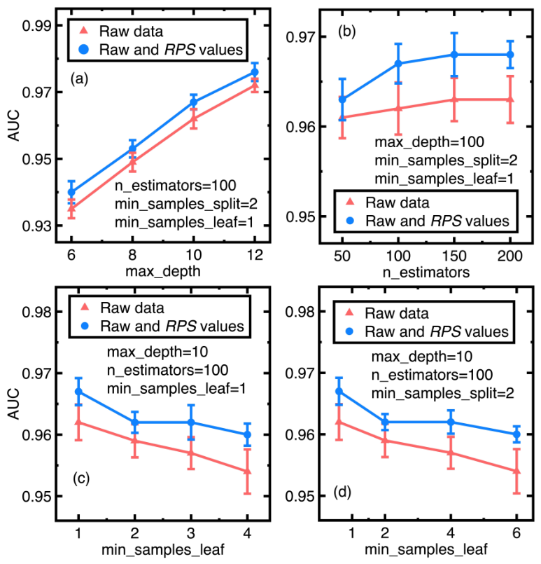
Training a random forest classifier requires the specification of several hyperparameters. Their effects on predictive performance must therefore be examined through a sensitivity analysis. Following the last paragraph of Section 3.2, this study evaluates four key hyperparameters: the maximum tree depth (max_depth), the number of trees in the forest (n_estimators), the minimum number of samples required to split an internal node (min_samples_split), and the minimum number of samples required at a leaf node (min_samples_leaf). Like Section 4.2, 18 random seeds are selected from the integer range of 30 to 80. For each seed, the reservoir water-quality data are randomly divided into training and test sets, with 75% of these data used for training and the remaining 25% reserved for testing. Random forest classifiers are trained with and without the inclusion of standardized features. Figure 7(a)-Figure 7(d) show the AUC values obtained under different hyperparameter settings. Each point represents the mean AUC across the 18 random seeds, whereas the error bars indicate the corresponding standard deviations.
Figure 7(a)-Figure 7(d) indicate that the AUC is most sensitive to the maximum tree depth (max_depth). In contrast, variations in the other hyperparameters have only modest effects on AUC performance. Furthermore, augmenting the reservoir water-quality data with -based features consistently improves the AUC across the evaluated hyperparameter settings.
5. Discussion
In light of the contributions stated in Section 1 and the numerical results presented in Section 4.1 and Section 4.2, the findings of this study are discussed as follows:
- The computation of in Equation (2) involves relatively few steps: calculating and identifying . Therefore, its computational procedure is more straightforward than those required for calculating Rousseeuw–Croux estimators and in Equations (11) and (12). This computational simplicity enhances the reproducibility and practical accessibility of the proposed measure.
- Augmenting the collected sensor data with -based features improves both macro-level and class-specific classification performance of a random forest classifier. Section 4.1, Section 4.2 and Section 4.3 show this improvement across three environmental sensor datasets subjected to different degrees of class imbalance. Although the improved macro-level and class-specific classification performance may be modest for both normal and anomalous sensor readings, it should be noted that these sensor readings were not collected over a short time period. Therefore, the enhanced macro-level and class-specific classification performance may reduce the risk of misinterpreting long-term environmental conditions. Surprisingly, the -based features enabled the random forest classifier to identify nearly all anomalous river-pollution events in Section 4.3. These results suggest that the proposed augmentation can provide useful evidence for environmental policymaking and regional governance.
- Calculating the robustly detects anomalous environmental measurements in Section 4.1, Section 4.2 and Section 4.3. Despite the accuracy of detected anomalies, calculating the Tukey interquartile range and Rousseeuw–Croux estimators and fails to detect extremely low conductivity, turbidity (in Section 4.2), and anomalous high air temperature (in Section 4.3). If we don’t understand the physical meaning of an environmental sensor measurement, it is difficult to determine which percentile rule should be imposed for locating the range of anomalous environmental sensor readings.
- Section 4.3 highlights the importance of explainability in evaluating classification performance. In this section, the recall for the class RPI ≤ 2 is lower than that for the class RPI > 2, suggesting that misclassified instances are more likely to occur in the former class. We further examine these misclassified cases to improve classification accuracy. However, because the official regulation does not define the river pollution index for the dataset used in this section, it is difficult to explain the misclassifications without augmenting the feature set with -based variables. Figure 2(a)–Figure 2(d), Figure 4(a)–Figure 4(d), and Figure 6(a)–Figure 6(d) show that may be a more effective anomaly measure for identifying the anomalous range of a variable than , , and , thereby providing a more interpretable basis for explaining misclassified instances.
6. Conclusions
This study applies a random forest classifier to classify air quality, reservoir water quality, and river water quality sensor data augmented with -based features. The serves as an anomaly measure to facilitate a random forest classifier in separating normal and anomalous data. To ensure the is an effective anomaly measure, additional tests show that it is a simpler and effective anomaly measure in comparison with the , , and . Furthermore, the improves the explainability of classification results. Referring to the corresponding values, we can understand why an instance is misclassified. Since we must avoid the target leakage in defining a class variable, raw data can’t provide similar explainability of misclassification results.
Conclusively, the contributions of this study are improving the weakness of a random forest classifier in classifying heavy-tailed data, demonstrating that the is a simple and effective anomaly measure, and enhancing the explainability of classification results provided by a random forest classifier. Based on these contributions, this study concludes:
- The provides a computational simple anomaly measure for identifying anomalous sensor readings. Its calculation requires fewer steps than the calculations of and . This computational simplicity enhances the reproducibility and practical accessibility of the proposed measure.
- The serves as an alternative anomaly measure for environmental monitoring data in which conventional mean- and standard-deviation-based measures may be sensitive to extreme values. Numerical results of this study show that it can identify anomalous observations in heavy-tailed environmental sensor datasets.
- Augmenting heavy-tailed environmental datasets with -based features improves the performance of a random forest classifier. The improvement was observed in both macro-level and class-specific classification results. After augmentation, the classifier made fewer classification errors for both normal and anomalous sensor readings, implying the reduce of misinterpreting long-time environmental conditions.
- The -based features can enhance the identification of rare but environmentally important events. The collected three datasets for implementing this study are subjected to different degrees of class imbalance. However, augmenting with -based features improves the accuracy in classifying all three datasets. In particular, the augmented classifier identified nearly all anomalous river-pollution events.
- The collected sensor data represented long-term environmental monitoring records. The proposed approach. Therefore, it may support environmental assessment, routine data screening, and evidence-based environmental policymaking.
However, the study may have several limitations. First, the collected data for implementing this study were sourced from environmental sensors. The generalizability of must be further examined using data from other types of sensors, monitoring locations, and sampling frequencies. Second, this study uses a random forest classifier to generate classification results. Future studies may evaluate the usefulness of -based features in other machine learning, such as the Naive-Bayes classifier. Investigating their use in real-time environmental monitoring systems is also suggested.
Author Contributions
This study is the author’s personal work.
Funding
This research received no external funding.
Data Availability Statement
’Air Quality’ at https://data.moenv.gov.tw/en/dataset/detail/AQX_P_434, ’Reservoir Water Quality’, and ’River Water Quality’ at https://wq.moenv.gov.tw/EWQP/zh/ConService/DownLoad/HistoryData.aspx (in traditional Chinese)
Conflicts of Interest
The authors declare no conflicts of interest.
Abbreviations
This manuscript includes the following abbreviations:
| AQI | Air quality index |
| AUC | Area under the curve |
| CTSI | Carlson’s trophic state index |
| IQR | Interquartile range |
| pH | Potential of hydrogen |
| RPI | River pollution index |
| RPS | Relative predictive surprise |
| SI | Surprise index |
References
- Liang, X.; Gao, Y.; Xu, S. ASE: Anomaly scoring based ensemble learning for highly imbalanced datasets. Expert Syst. Appl. 2024, 238, 122049. [CrossRef]
- O’Brien, R.; Ishwaran, H. A random forests quantile classifier for class imbalanced data. Pattern Recognit. 2019, 90, 232–249. [CrossRef]
- Bayarri, M.J.; Morales, J. Bayesian measures of surprise for outlier detection. J. Stat. Plan. Infer. 2003, 111(1), 3–22. [CrossRef]
- Rousseeuw, P.J.; Croux, C. Alternatives to the median absolute deviation. J. Am. Stat. Assoc. 1993, 88(424), 1273–1283. [CrossRef]
- Tukey, J.W.Exploratory Data Analysis, Pearson: New York, USA, 1977.
- Harvey, J.S.; Rosaler, J., Li, M.; Desai, D.; Mehta, D. Explainable unsupervised anomaly detection with random forest. arXiv 2025, arXiv:2504.16075.
- Hill, B.M. A simple general approach to inference about the tail of a distribution. Ann. Stat. 1975, 3(5), 1163–1174. [CrossRef]
- Bhattacharya, S.; Kallitsis, M.; Stoev, S. Data-adaptive trimming of the Hill estimator and detection of outliers in the extremes of heavy-tailed data. Electron. J. Stat. 2023, 19(1), 1872–1925.
- Bhattacharya, S.; Kamper, F.; Beirlant, J. Outlier detection based on extreme value theory and applications. Scand. J. Stat. 2019, 13(1), 1872–1925.
- Verardi, V.; Vermandele, C. Univariate and multivariate outlier identification for skewed or heavy-tailed distributions. Stata J. 2018, 18, 517–532. [CrossRef]
- Li, Z.; Zhao, Y.; Hu, X.; Botta, N.; Ionescu, C.; Chen, G.H. ECOD: Unsupervised outlier detection using empirical cumulative distribution functions. IEEE Trans. Knowl. Data Eng. 2023, 35(12), 12181–12193. [CrossRef]
- Horváth, G.; Kovács, E. Molontay, R. Nováczki, S. Copula-based anomaly scoring and localization for large-scale, high-dimensional continuous data. ACM Trans. Intell. Syst. Technol. 2019, 11, 1–26. [CrossRef]
- Bourigault, P.; Mandic, D. Kernel-based anomaly detection using generalized hyperbolic processes. In 2025 IEEE International Conference on Acoustics, Speech and Signal Processing (ICASSP 2025), Hyderabad, India, 6-11 April 2025; pp. 1–5.
- Tortora, C.; Punzo, A.; Franczak, B. Handling skewness and directional tails in model-based clustering. Stat. Pap. 2025, 66, 114. [CrossRef]
- Zenati, H.; Romain, M.; Foo, C.-S.; Lecouat, B.; Chandrasekhar, V. Adversarially learned anomaly detection. In 2018 IEEE International Conference on Data Mining (ICDM), Singapore, Singapore, 17-20 November 2018; pp. 727–736.
- Dionelis, N. Tail of distribution GAN (TailGAN): Generative adversarial-network-based boundary formation. In 2020 Sensor Signal Processing for Defence Conference (SSPD), Edinburgh, UK, 15-16 September 2020; pp. 1–5.
- Yang, C.-A.; Peng, K.-C.; Yeh, R. Toward long-tailed online anomaly detection through class-agnostic concepts. arXiv 2025, arXiv:2507.16946.
- Ma, Y.; Jiao, L.; Liu, F.; Yang, S.; Liu, X.; Chen, P. Geometric prior guided feature representation learning for long-tailed classification. Int. J. Comput. Vis. 2024, 132(7), 2493–2510. [CrossRef]
- Song, Y.; Li, M.; Wang, B. A long-tailed image classification method based on enhanced contrastive visual language. Sensors 2023, 23(15), 6694. [CrossRef]
- Delaigle, A.; Hall, P. Effect of heavy tails on ultra high dimensional variable ranking methods. Stat. Sinica 2012, 22, 909–932. [CrossRef]
- Good, I.J. The surprise index for the multivariate normal distribution Ann. Math. Stat. 1956, 27(4), 1130–1135. [CrossRef]
- Weaver, W. Probability, rarity, interest and surprise, Sci. Monthly 1948, 67(6), 390–392.
- Kullback, S.; Leibler, R.A. On information and sufficiency, Ann. Math. Stat. 1951, 22(1), 79–86. [CrossRef]
- Rogers, J. How “random” is ryanair’s seating allocation?, Signif. 2017, 14(5), 12–13. [CrossRef]
- Breiman, L.; Friedman, J.; Stone, C.J.; Olshen, R.A. Classification and Regression Trees, Chapman and Hall/CRC: New York, USA, 1984.
- Cutler, A.; Cutler, D.R.; Stevens, J.R. Random forests. In Ensemble Machine Learning: Methods and Applications; Zhang, C.; Ma, Y., Eds.; Springer: New York, USA, 2012; pp. 157–175.
- Air quality data. 2026-01-01: https://data.moenv.gov.tw/en/dataset/detail/AQX_P_434.
- Reservoir water quality. 2026-03-30: https://wq.moenv.gov.tw/EWQP/en/Default.aspx (in traditional Chinese).
- Carlson, R.E. A trophic state index for lakes, Limnol. Oceanogr. 1977, 22(2), 361–369. [CrossRef]
Figure 1.
Distributions of the collected air quality data
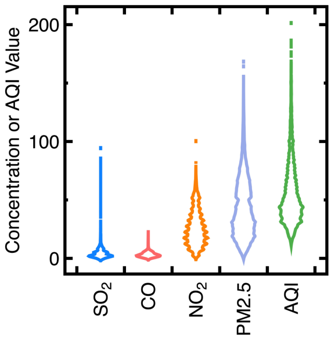
Figure 2.
Comparisons of anomalies in the collected air quality data identified using the , , , , and a 90th percentile rule
Figure 2.
Comparisons of anomalies in the collected air quality data identified using the , , , , and a 90th percentile rule
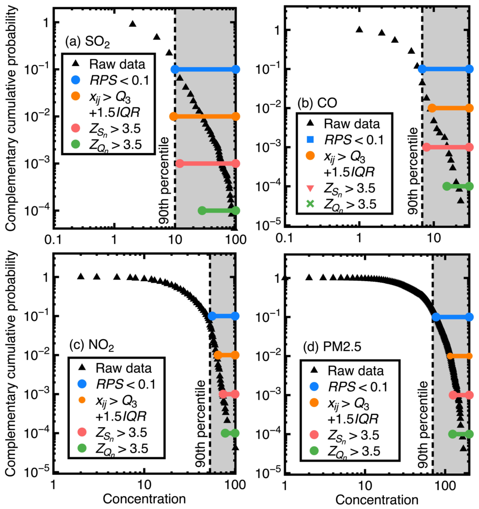
Figure 3.
Distributions of the collected reservoir water quality data
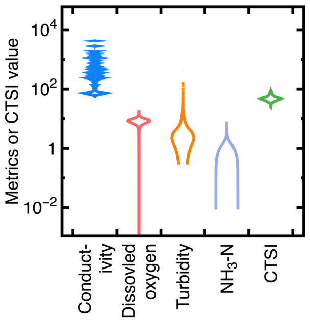
Figure 4.
Comparisons of anomalies in the collected reservoir water quality data identified using the , , , , 90th, 10th, and 5th percentile rules)
Figure 4.
Comparisons of anomalies in the collected reservoir water quality data identified using the , , , , 90th, 10th, and 5th percentile rules)
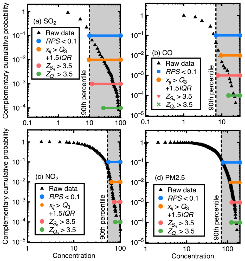
Figure 5.
Distributions of the collected river water quality data
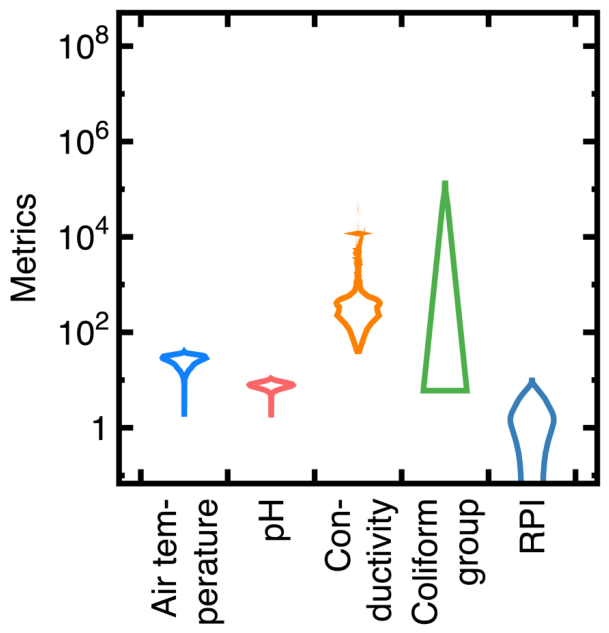
Figure 6.
Comparisons of anomalies in the collected river water quality data identified using the , , , , 90th and 5th percentile rules
Figure 6.
Comparisons of anomalies in the collected river water quality data identified using the , , , , 90th and 5th percentile rules
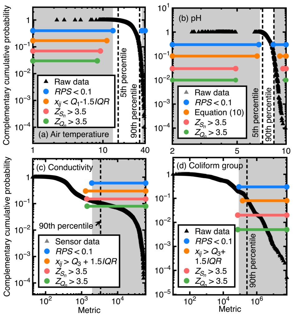
Figure 7.
Effects of four selected hyperparameters on the performance of a random forest classifier with and without augmenting -based features
Figure 7.
Effects of four selected hyperparameters on the performance of a random forest classifier with and without augmenting -based features

| Interpretation | ||
| Normal | ||
| Marginally anomalous | ||
| Moderately anomalous | ||
| Seriously anomalous |
Table 2.
Descriptive statistics of the collected air quality data
| Statistics | SO2 | CO | NO2 | PM2.5 | AQI |
| Mean | 4.706 | 3.105 | 25.96 | 43.341 | 54.47 |
| Median | 2 | 3 | 23 | 38 | 48 |
| Mode | 2 | 2 | 17 | 31 | 44 |
| Range | [0,95] | [0,23] | [0,101] | [0,169] | [9,202] |
| Variance | 29.699 | 3.637 | 215.83 | 636.474 | 643.176 |
| Standard deviation | 5.449 | 1.907 | 14.691 | 25.228 | 25.36 |
| 3 | 3 | 20 | 37 | 31 | |
| Skewness | 4.853 | 1.308 | 0.606 | 0.785 | 1.221 |
| Kurtosis | 41.781 | 3.928 | -0.272 | 0.415 | 1.707 |
| 11.567 | 25.899 | 5.524 | 48.064 | 14.921 |
Table 3.
Interpretation of the trimmed Hill index [8]
Table 3.
Interpretation of the trimmed Hill index [8]
| Interpretation | |
| ≈ 0 | No clear heavy-tail evidence |
| 0.2-0.5 | Heavy tail |
| > 0.5 | Very heavy tail |
| Extreme tail heaviness |
Table 4.
Classification performance of air quality data before and after -based augmentation
| Metric | Raw data | Raw data and values | |
| AUC | |||
| Macro F1-score | |||
| Weighted F1-score | |||
| Accuracy | |||
| Weighted specificity | |||
| Weighted precision | |||
| Recall | AQI | ||
| AQI | |||
| AQI | |||
Note: each classification metric is presented in its mean and standard deviation.
Table 5.
Descriptive statistics of the collected reservoir water quality data
| Statistics | Conductivity | Dissolved oxygen | Turbidity | NH3−N | CTSI |
| Mean | 388.878 | 8.535 | 6.228 | 0.817 | 50.014 |
| Median | 320 | 8.4 | 3.3 | 0.03 | 48 |
| Mode | 72 | 8.2 | 1.9 | 0.02 | 46 |
| Range | [59, 7980] | [0, 18.4] | [0.3, 550] | [0.0086, 6.94] | [25, 88] |
| Variance | 122,053.2 | 2.569 | 224.161 | 0.102 | 105.598 |
| STD | 394.334 | 1.603 | 14.971 | 0.319 | 10.275 |
| 186 | 1.5 | 4.4 | 0.03 | 11 | |
| Skewness | 6.928 | 0.479 | 22.017 | 11.043 | 1.046 |
| Kurtosis | 95.007 | 4.857 | 691.243 | 155.326 | 1.041 |
| 2.09 | 34.728 | 3.615 | 4.27 | 100.737 |
Table 6.
Classification performance of reservoir water quality data before and after -based augmentation
Table 6.
Classification performance of reservoir water quality data before and after -based augmentation
| Metric | Raw data | Raw data and values | |
| AUC | |||
| Macro F1-score | |||
| Weighted F1-score | |||
| Accuracy | |||
| Weighted specificity | |||
| Weighted precision | |||
| Recall | CTSI < 40 | ||
| CTSI | |||
| CTSI | |||
Note: each classification metric is presented in its mean and standard deviation.
Table 7.
Descriptive description of the collected river water quality data
| Statistics | Air temperature | pH | Conductivity | Coliform group | RPI |
| Mean | 26.812 | 7.864 | 2,457.846 | 152,431 | 2.799 |
| Median | 27.8 | 7.9 | 442 | 14,000 | 2.25 |
| Mode | 32 | 8.2 | 410 | 21,000 | 1 |
| Range | [2.2, 38.8] | [2.64, 9.9] | [44, 52,300] | [10, 6.2] | [1,10] |
| Variance | 31.256 | 0.301 | 51,413,848.01 | 1.17 | 3.418 |
| STD | 5.591 | 0.549 | 7,170.166 | 1,081,075 | 1.849 |
| 7.9 | 0.63 | 401 | 56,300 | 3 | |
| Skewness | -0.612 | -2.646 | 4.219 | 31.416 | 0.846 |
| Kurtosis | -0.198 | 17.745 | 18.149 | 1338.833 | -0.144 |
| 222.775 | 57.4 | 255.86 | 8.819 | 20.833 |
Table 8.
Classification performance of river water quality data with and without -based augmentation
Table 8.
Classification performance of river water quality data with and without -based augmentation
| Metric | Raw data | Raw and values | |
| AUC | |||
| Macro F1-score | |||
| Weighted F1-score | |||
| Accuracy | |||
| Weighted specificity | |||
| Weighted precision | |||
| Recall | RPI ≤ 2 | ||
| RPI >2 | |||
Note: each classification metric is presented in its mean and standard deviation.
Disclaimer/Publisher’s Note: The statements, opinions and data contained in all publications are solely those of the individual author(s) and contributor(s) and not of MDPI and/or the editor(s). MDPI and/or the editor(s) disclaim responsibility for any injury to people or property resulting from any ideas, methods, instructions or products referred to in the content. |
© 2026 by the authors. Licensee MDPI, Basel, Switzerland. This article is an open access article distributed under the terms and conditions of the Creative Commons Attribution (CC BY) license (http://creativecommons.org/licenses/by/4.0/).
Copyright: This open access article is published under a Creative Commons CC BY 4.0 license, which permit the free download, distribution, and reuse, provided that the author and preprint are cited in any reuse.