

Submitted:
11 August 2026
Posted:
12 August 2026
You are already at the latest version
Abstract
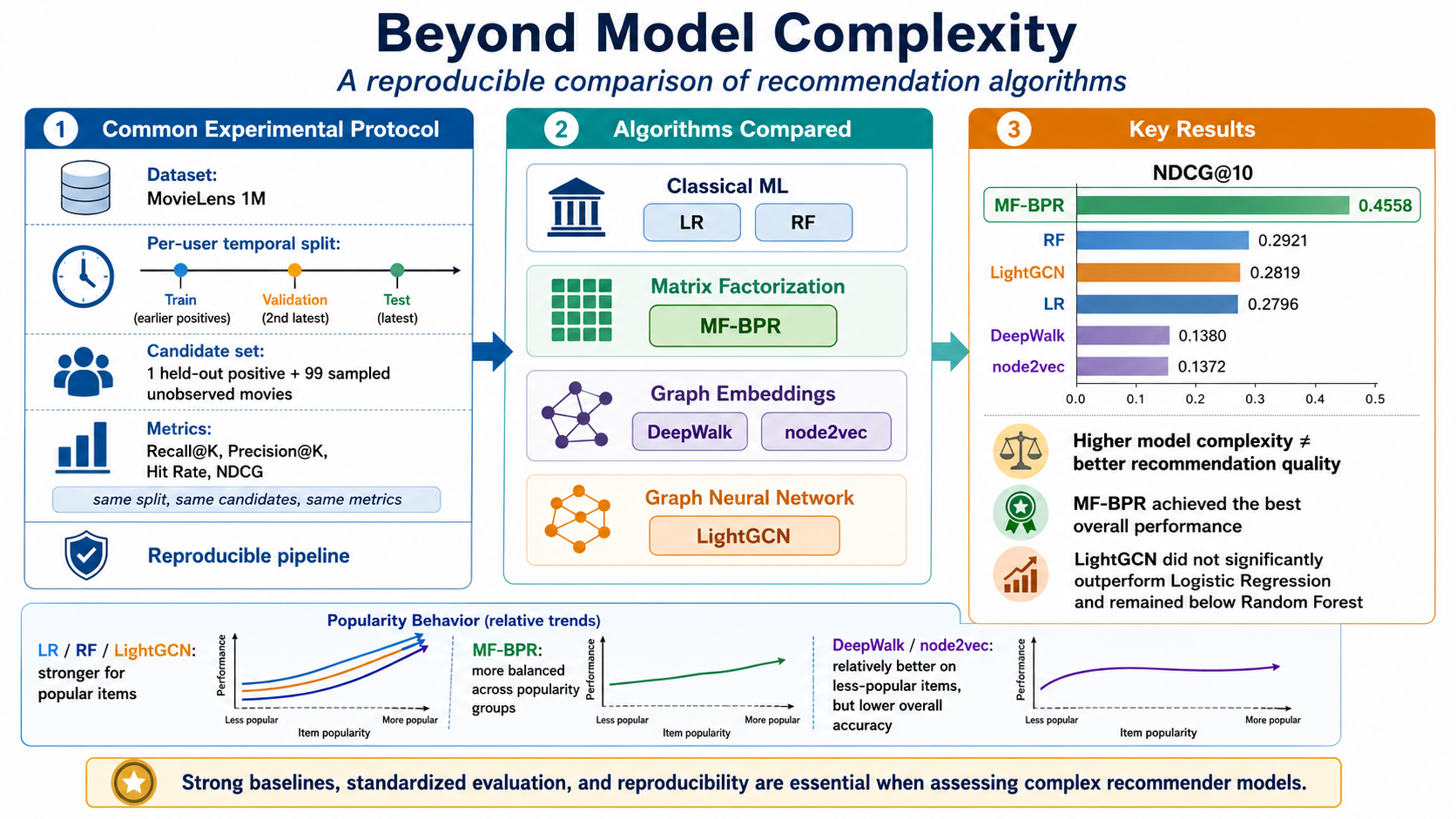
Recommender systems increasingly incorporate graph embeddings and graph neural networks to capture high-order relationships between users and items. However, the additional complexity of these approaches does not necessarily guarantee better recommendation quality than strong classical and latent-factor baselines. This study presents a reproducible comparison of six recommendation models representing four methodological families: Logistic Regression, Random Forest, Matrix Factorization with Bayesian Personalized Ranking, DeepWalk, node2vec, and LightGCN. The experiments were conducted on the MovieLens 1M dataset using a per-user temporal split. For each user, the most recent positive interaction was assigned to testing, the preceding interaction to validation, and all earlier positive interactions to training. All models were evaluated using identical candidate sets containing one held-out positive movie and 99 sampled unobserved movies. Performance was measured using Recall, Precision, Hit Rate, and NDCG at multiple cutoffs, complemented by bootstrap confidence intervals, paired statistical tests, computational-efficiency measurements, and analyses by user activity and movie popularity. Matrix Factorization achieved the best overall performance, reaching a Recall@10 of 0.7458 and an NDCG@10 of 0.4558, representing an approximately 56% improvement in NDCG@10 over Random Forest, the strongest classical baseline. LightGCN did not significantly outperform Logistic Regression and remained below Random Forest, despite its higher computational cost. DeepWalk and node2vec obtained similar and substantially lower aggregate results. Popularity-based analysis further revealed that classical models and LightGCN achieved substantially higher ranking effectiveness for popular movies, whereas Matrix Factorization maintained comparatively stronger performance for less-popular items. These findings demonstrate that model complexity alone is not a reliable indicator of recommendation effectiveness and highlight the importance of strong baselines, standardized evaluation, and reproducible experimental protocols.
Keywords:
recommender systems
; matrix factorization
; graph neural networks
; graph embeddings
1. Introduction
The rapid growth of digital content has made it increasingly difficult for users to identify relevant products, services, and information. Recommender systems address this problem by estimating user preferences and producing personalized rankings of candidate items. Their applications extend across domains such as electronic commerce, digital media, social platforms, and online education. From a computational perspective, recommendation can be formulated as the prediction of preferences or as a personalized ranking problem in which relevant items should appear at the highest possible positions.
Collaborative filtering remains one of the most influential paradigms for recommendation because it exploits interaction patterns without requiring a complete semantic description of users and items. Among collaborative approaches, matrix factorization has been particularly successful because it represents users and items in a shared low-dimensional latent space [1]. For implicit-feedback recommendation, Bayesian Personalized Ranking (BPR) provides a pairwise learning criterion that directly encourages observed items to receive higher scores than unobserved alternatives [2]. These methods are conceptually simple, computationally efficient, and continue to constitute strong baselines for evaluating more complex recommendation architectures.
More recently, user–item interactions have increasingly been represented as bipartite graphs. This formulation makes relationships explicit and enables the application of graph representation learning. Random-walk methods such as DeepWalk learn node embeddings by treating truncated graph walks as sequences analogous to sentences [3]. node2vec extends this idea through biased random walks that balance local and outward exploration of network neighborhoods [4]. Graph neural networks go further by propagating information through adjacent nodes. In particular, LightGCN removes feature transformations and nonlinear activations from conventional graph convolutional networks and retains neighborhood aggregation as the central operation for collaborative filtering [5].
Although graph-based and neural recommendation models provide increasingly sophisticated mechanisms for learning relational patterns, greater architectural complexity does not necessarily imply better recommendation quality. Previous reproducibility studies have shown that several neural recommendation proposals do not consistently outperform well-tuned traditional methods and that conclusions can depend substantially on baseline selection and experimental configuration [6]. Consequently, comparisons between classical machine learning, latent-factor methods, graph embeddings, and graph neural networks should be conducted under a shared and reproducible protocol rather than relying on results obtained from heterogeneous data partitions, candidate sets, or evaluation procedures.
In this study, model complexity refers primarily to architectural and representational sophistication, including the transition from feature-based models and latent-factor methods to random-walk graph embeddings and graph neural recommendation. It does not denote a formal computational-complexity analysis, parameter-count comparison, or asymptotic runtime characterization. Computational cost is examined separately through training and inference time.
Evaluation design is particularly important in top-K recommendation. Random data partitions may allow future interactions to influence model training and therefore produce optimistic estimates of performance. Temporal partitions offer a more realistic setting by requiring models to predict later interactions from earlier user behavior. Candidate construction is also consequential. Sampling a limited number of unobserved items reduces computational cost, but sampled ranking metrics may not preserve the same relative ordering between algorithms as full-catalog evaluation [7]. Therefore, candidate generation, negative sampling, temporal ordering, and metric computation must be applied consistently across all compared models and explicitly reported.
This study presents a reproducible comparison of six recommendation approaches representing four methodological families: Logistic Regression and Random Forest as feature-based classical machine-learning models; Matrix Factorization optimized with BPR as a latent-factor method; DeepWalk and node2vec as random-walk graph-embedding methods; and LightGCN as a graph neural recommender. The experiments use the MovieLens 1M dataset, a widely adopted benchmark containing user ratings and demographic and movie-related information [8]. Explicit ratings equal to or greater than four are interpreted as positive interactions, and a per-user temporal strategy assigns the last positive interaction to testing, the preceding interaction to validation, and all earlier positive interactions to training.
All methods are evaluated using the same held-out users and the same candidate sets. Each test candidate set contains one temporally held-out positive movie and 99 reproducibly sampled unobserved movies. Recommendation quality is measured using Recall, Precision, Hit Rate, and Normalized Discounted Cumulative Gain at multiple cutoffs. The analysis also considers user-level bootstrap confidence intervals, paired statistical comparisons, training and inference costs, user activity, and the popularity of the held-out movie. This common protocol makes it possible to examine whether explicitly modeling the user–item graph provides consistent benefits over simpler alternatives.
The main contributions of this work are as follows:
- A reproducible experimental framework that compares classical machine learning, matrix factorization, graph embeddings, and graph neural recommendation under the same temporal partitions and candidate sets.
- An empirical analysis showing that increasing model complexity does not necessarily improve recommendation quality, with BPR-based Matrix Factorization outperforming the evaluated feature-based and graph-based alternatives on the adopted protocol.
- A user-level statistical analysis based on bootstrap confidence intervals, the Friedman test, Wilcoxon signed-rank comparisons, Holm correction, and effect-size estimation.
- An analysis of computational efficiency and recommendation behavior across user-activity and movie-popularity groups, revealing substantial differences in how the evaluated models handle popular and less-popular items.
- A complete workflow that preserves processed data, fixed candidate sets, trained models, predictions, metrics, statistical results, and publication-ready tables and figures.
The remainder of this paper is organized as follows. Section 2 reviews classical collaborative filtering, graph embeddings, and graph neural recommendation. Section 3 describes the dataset, temporal partitioning, evaluated models, and evaluation protocol. Section 4 presents the experimental results. Section 5 discusses their implications and limitations. Finally, Section 6 summarizes the main findings and outlines future research directions.
2. Related Works
2.1. Evolution of Recommender-System Approaches
Recommender systems have evolved from neighborhood-based collaborative filtering and latent-factor methods toward deep learning, graph representation learning, self-supervised learning, and hybrid architectures. Recent surveys describe a broad methodological landscape that includes collaborative filtering, content-based approaches, deep neural networks, knowledge graphs, graph neural networks, reinforcement learning, and emerging large-language-model approaches [9,10]. Despite this expansion, traditional methods such as k-nearest neighbors, singular value decomposition, and matrix factorization remain widely used because of their relative simplicity, scalability, and competitive predictive performance [10].
Matrix factorization continues to be a particularly important reference point for collaborative recommendation. It represents users and items in a shared latent space and can be adapted to both rating prediction and personalized ranking. Its flexibility has also enabled extensions beyond conventional single-item recommendation. For example, Hurtado Ortiz et al. proposed a clustering-based recommender system that applies matrix factorization to bundle recommendation for individual users and user communities [11]. In a related direction, Bobadilla et al. introduced a Bayesian non-negative matrix factorization approach for clustering users and items in sparse rating matrices. Their experiments across multiple open datasets reported improved clustering quality compared with classical matrix factorization and enhanced K-means, while also showing competitive prediction accuracy and execution time [12]. Recent comparative evidence further indicates that latent-factor models remain competitive even when evaluated against neural alternatives. For example, Rodríguez-López et al. compared progressively more complex rating and ranking models on an Amazon dataset and found that matrix factorization and Bayesian Personalized Ranking achieved strong results, while neural models were competitive only under particular data characteristics and tuning conditions [13]. These findings reinforce the need to treat model complexity as an empirical design choice rather than as an automatic indicator of superior recommendation quality.
Beyond conventional latent-factor formulations, neural architectures have also been used to learn item representations with properties similar to matrix-factorization embeddings. Shanthakumar et al. proposed an item-based recommendation approach in which deep networks generate item embeddings that can subsequently be used to compute recommendations. Their work illustrates an intermediate design between traditional matrix factorization and fully neural recommender architectures, in which latent item representations remain central to the recommendation process [14].
2.2. Graph Embeddings and Graph Neural Recommendation
User–item interactions can be naturally represented as bipartite graphs, in which users and items are nodes and observed interactions are edges. This representation enables models to exploit relational structure beyond independent user–item observations. Random-walk graph-embedding methods learn node representations from sequences generated by traversing the interaction graph, whereas graph neural networks propagate information through neighboring nodes and can capture increasingly high-order connectivity patterns.
Recent literature presents graph neural networks as a major direction in recommendation because they can model local and global dependencies in user–item graphs and incorporate auxiliary information [15,16]. Existing approaches include graph convolutional networks, graph attention networks, GraphSAGE variants, graph-transformer architectures, contrastive-learning methods, and simplified collaborative-filtering models. For example, Verma et al. applied GraphSAGE to a bipartite user–book interaction graph constructed from the Book-Crossing dataset. Their approach aggregated neighboring-node information together with book metadata and user demographic attributes to learn representations for rating prediction, reporting an RMSE of 0.4818, an MSE of 0.2321, and an MAE of 0.2872 [17]. This application illustrates the capacity of neighborhood-aggregation models to combine interaction structure and auxiliary information in domain-specific recommendation settings. A recent survey of graph-based collaborative filtering identifies data sparsity, cold start, oversmoothing, fairness, and scalability as persistent challenges, while also highlighting self-supervised learning, multimodal information, and large language models as emerging research directions [16].
However, the effectiveness of graph neural architectures is strongly dependent on the interaction graph, available node features, and application domain. Nanupatruni et al. evaluated several GNN architectures across datasets from anime, e-commerce, video games, and movie recommendation and reported substantial variation between domains [18]. GraphSAGE and adaptive graph-convolution methods were comparatively robust in dense settings, whereas attention-based architectures were more competitive when informative features were available. Consequently, evidence obtained from one benchmark or one graph structure cannot be assumed to generalize to other recommendation domains.
2.3. Complexity and the Strength of Traditional Baselines
Although graph-based models have greater representational capacity, recent research does not establish that they consistently outperform simpler alternatives. Comparative and tertiary studies indicate that performance depends on dataset density, interaction patterns, recommendation objective, baseline implementation, and hyperparameter tuning [10,13]. Advanced architectures may capture high-order relationships, but this benefit must be weighed against their additional optimization requirements, memory consumption, and computational cost.
This issue is particularly important when model families are evaluated under different experimental conditions. A neural or graph model may appear superior when compared with weakly tuned baselines, different data partitions, or different candidate sets. Conversely, strong matrix-factorization and feature-based models may remain competitive when all methods receive comparable tuning and are evaluated using the same ranking protocol. Therefore, fair comparisons require not only a diverse model set but also standardized data splits, negative-sampling procedures, candidate construction, and metrics.
2.4. Reproducibility and Evaluation Methodology
Reproducibility has become a central concern in recommender-systems research. Ferrari Dacrema et al. analyzed graph-based recommender-system papers based on message passing and identified erroneous data partitions, information leakage, inconsistencies between manuscripts and released artifacts, and the use of complex but comparatively weak baselines [19]. Their reproduction study was unable to confirm several of the original claims, illustrating that reported improvements may depend on implementation and evaluation choices rather than on the proposed architecture alone.
The problem extends beyond source-code availability. Reproducible evaluation requires the exact preservation of preprocessing decisions, interaction thresholds, train–validation–test partitions, sampled negatives, candidate sets, trained parameters, and metric implementations. Temporal evaluation is particularly relevant because random partitions can allow later user behavior to influence training, producing an optimistic estimate of future recommendation performance. Nevertheless, recent surveys note that temporal evaluation and ranking protocols remain heterogeneous across graph-based collaborative-filtering studies [16].
Evaluation based on sampled candidate sets also requires careful interpretation. A model evaluated against a small set of sampled unobserved items is not solving exactly the same task as a model ranking the complete item catalog. Although sampled evaluation reduces computational cost and facilitates controlled comparison, results can depend on the number and distribution of sampled negatives. Accordingly, candidate generation should be identical for every model and clearly distinguished from full-ranking evaluation.
2.5. Popularity Bias, Fairness, and Long-Tail Recommendation
Accuracy metrics alone do not fully characterize recommendation behavior. Modern surveys emphasize robustness, data bias, fairness, and exposure as important dimensions of recommender-system evaluation [9]. Popularity bias is especially relevant because interaction datasets are typically concentrated around a relatively small number of popular items. Models trained on such data may reinforce existing exposure patterns, improve aggregate accuracy, and simultaneously provide limited visibility to less-popular items.
Chizari et al. examined bias amplification in GNN-based recommender systems and showed that graph-based methods should be assessed not only by predictive performance but also by their influence on pre-existing biases [20]. The graph structure can propagate popularity and exposure effects through multiple neighborhoods, potentially amplifying imbalances already present in the training data. This concern motivates analyses that separate performance for popular and long-tail items rather than reporting only aggregate ranking metrics.
Despite growing recognition of fairness and popularity bias, direct head-to-head evidence across classical machine learning, matrix factorization, random-walk embeddings, and graph neural networks remains limited. Existing surveys synthesize broad methodological trends, while many empirical studies focus on variants within a single family. Consequently, it remains unclear whether the relational capacity of graph-based models produces consistent advantages for both popular and less-popular items under a common temporal evaluation protocol.
2.6. Research Gap
The reviewed literature identifies three unresolved issues. First, there is limited empirical comparison across fundamentally different model families under identical partitions, candidate sets, and ranking metrics. Second, the greater complexity of graph-based and neural architectures has not been shown to produce consistent improvements over well-established latent-factor and classical baselines. Third, reproducibility, computational efficiency, and popularity-dependent behavior are often analyzed separately rather than within one experimental framework.
This study addresses these gaps through a reproducible comparison of Logistic Regression, Random Forest, BPR-based Matrix Factorization, DeepWalk, node2vec, and LightGCN. All models use a common per-user temporal split and identical validation and test candidate sets. In addition to top-K effectiveness, the study examines confidence intervals, paired statistical differences, computational cost, user activity, and held-out item popularity. The objective is not to assume the superiority of graph-based recommendation, but to determine whether its additional relational complexity provides measurable benefits under a common temporal and sampled-ranking protocol.
3. Methods
3.1. Research Design
This study follows a controlled comparative experimental design to evaluate recommendation approaches from four methodological families: feature-based classical machine learning, latent-factor models, graph embeddings, and graph neural networks. The evaluated methods are Logistic Regression, Random Forest, Matrix Factorization with Bayesian Personalized Ranking, DeepWalk, node2vec, and LightGCN.
The comparison was designed to reduce evaluation-related confounding across model families. Accordingly, all methods used the same dataset, positive-interaction definition, temporal partition, eligible users, validation candidates, test candidates, ranking cutoffs, and metric implementations.
The complete experimental workflow was implemented as a sequence of reproducible Jupyter notebooks. The source code, environment specifications, configuration files, and execution instructions are available in a public GitHub repository:
3.2. Dataset
The experiments used the MovieLens 1M dataset, a widely adopted benchmark for recommender-system research [8]. The dataset contains approximately one million explicit ratings assigned by users to movies, as well as demographic attributes for users and descriptive information for movies.
Each interaction is represented as a tuple
where u denotes a user, i a movie, r the explicit rating, and t the interaction timestamp. Ratings greater than or equal to four were interpreted as positive implicit-feedback interactions:
Only positive interactions were used to construct the temporal train, validation, and test partitions. However, every observed user–movie pair, including ratings below four, was excluded from negative sampling. This decision prevented known interactions from being incorrectly treated as unobserved negative examples.
3.3. Temporal Interaction Split
A per-user chronological splitting strategy was adopted to approximate the task of predicting future user preferences. Positive interactions were sorted by timestamp independently for each user. Users with fewer than three positive interactions were excluded because at least one interaction was required for each of the training, validation, and test subsets.
For every eligible user:
- the most recent positive interaction was assigned to the test set;
- the second most recent positive interaction was assigned to the validation set;
- all earlier positive interactions were assigned to the training set.
Let the chronologically ordered positive interactions of user u be
The resulting partition is defined as
This strategy guarantees that validation and test interactions occur after the interactions used for training.
3.4. Feature-Based Classical Machine-Learning Models
Logistic Regression and Random Forest were used as feature-based classical baselines. Each user–movie pair was treated as an independent observation, without graph propagation or learned graph neighborhoods.
The pair representation concatenated:
- user profile attributes provided by MovieLens;
- movie profile attributes provided by MovieLens;
- logarithmic user activity;
- logarithmic movie popularity;
- normalized user activity;
- normalized movie popularity;
- mean user rating in the training set;
- mean movie rating in the training set;
- logarithm of the user-degree and movie-degree product;
- absolute difference between normalized user and movie degrees;
- absolute difference between user and movie mean ratings.
All aggregate statistics were computed exclusively from training interactions. Therefore, no validation or test information was used during feature construction.
For every positive training interaction, one unobserved user–movie pair was sampled as a negative example. The sampling process excluded every pair observed in the original dataset.
Logistic Regression was trained after standardizing the input features. The classifier used the lbfgs optimizer and a maximum of 500 iterations. Random Forest used 100 trees, unrestricted maximum depth, a minimum of two samples per leaf, balanced class weights, and parallel CPU execution.
3.5. Matrix Factorization with BPR
Matrix Factorization represents every user and movie through a latent vector of dimension d. The score assigned to a pair is the inner product
where is the user embedding and is the movie embedding [1].
The model was optimized using Bayesian Personalized Ranking [2]. For each training triplet , where i is an observed positive movie and j is a sampled unobserved movie, the objective encourages
The BPR loss is
where is the sigmoid function.
The model used 64-dimensional embeddings, a batch size of 4096, a learning rate of , and weight decay of . Training was limited to 100 epochs. Early stopping was applied with a patience of 10 epochs and a minimum improvement of in validation NDCG@10.
3.6. Graph Construction
The positive training interactions were represented as an undirected bipartite graph
where is the set of users, is the set of movies, and
Validation and test edges were not included in the graph. This same training graph was used by DeepWalk, node2vec, and LightGCN.
3.7. DeepWalk
DeepWalk learns node representations by generating unbiased random walks and treating them as sequences for Skip-gram training [3]. Walks were initiated from every active node in the bipartite graph.
The experimental configuration used:
- embedding dimension: 64;
- number of walks per active node: 10;
- walk length: 40;
- Skip-gram context window: 5;
- negative samples: 5;
- Word2Vec training epochs: 5.
A single worker was used during Word2Vec training to improve determinism. After training, user and movie embeddings were normalized by their Euclidean norm. Recommendation scores were calculated using cosine similarity:
3.8. node2vec
node2vec extends random-walk embedding by introducing second-order transition probabilities controlled by the return parameter p and the in–out parameter q [4].
Given the previous node t, current node v, and candidate next node x, the unnormalized transition weight is
The implementation used and , producing a bias toward outward graph exploration. All remaining parameters were identical to those used for DeepWalk: 64-dimensional embeddings, 10 walks per node, walk length 40, context window 5, five negative samples, and five Word2Vec epochs.
Recommendation scores were obtained from the cosine similarity between the normalized user and movie embeddings.
3.9. LightGCN
LightGCN was selected as the graph-neural recommendation model because it removes feature transformations and nonlinear activations from conventional graph convolution and retains only neighborhood propagation [5].
Let and denote the initial trainable embeddings of user u and movie i. At propagation layer , the embeddings are updated as
The final representation is the mean of the embeddings obtained from the initial layer and all propagation layers:
The user–movie score is
The model used 64-dimensional embeddings and three propagation layers. Optimization used Adam with a learning rate of , weight decay of , and the BPR objective. Training was performed in full-batch mode for at most 100 epochs. Early stopping used validation NDCG@10, a patience of 10 epochs, and a minimum improvement of .
3.10. Candidate Generation
Validation and test candidate sets were generated independently but with the same procedure. For every eligible user, the candidate set contained:
- one temporally held-out positive movie;
- 99 reproducibly sampled unobserved movies.
Thus, each candidate set contained exactly 100 movies per user. Negative movies were sampled uniformly from movies for which no rating from the user was recorded in the complete dataset. Duplicates were not allowed within a user’s candidate set.
The same validation candidate set was used for model selection and early stopping across all methods. Similarly, the same test candidate set was used for the final evaluation of every model. Candidate generation used a fixed random seed and the resulting files were persisted to guarantee that all models were evaluated under identical conditions.
3.11. Evaluation Metrics
The models were evaluated at . Since each user had exactly one relevant movie in the candidate set, Recall@K and Hit Rate@K coincide numerically. Both are retained to facilitate comparison with the recommender-systems literature.
For user u, Recall@K is
where is the set of the top-K recommended movies and is the held-out relevant set.
Precision@K is
Hit Rate@K is
Normalized Discounted Cumulative Gain is
with
Because one binary relevant item was used per user, the ideal discounted gain was equal to one. Ties in predicted scores were resolved deterministically by sorting first by descending score and then by ascending movie index.
3.12. Statistical Analysis
User-level bootstrap confidence intervals were calculated for every ranking metric. Users were sampled with replacement 1,000 times, and the 2.5th and 97.5th percentiles of the bootstrap distribution were reported as the 95% confidence interval.
Differences among all models were first examined using the Friedman test, treating users as blocks and models as repeated measurements. Kendall’s coefficient of concordance W was reported as a global effect-size measure.
When the omnibus comparison was significant, two-sided Wilcoxon signed-rank tests were performed for every model pair using user-level NDCG@10 values. Holm correction was applied to control the family-wise error rate. Rank-biserial correlation was additionally reported as a pairwise effect-size indicator.
These analyses quantify variation and paired differences across users under a fixed experimental realization. They do not estimate variability caused by retraining the models with multiple random seeds.
3.13. Activity, Popularity, and Efficiency Analyses
To examine whether model behavior depended on the amount of available user history, users were divided into quartiles according to their number of positive training interactions. Recall@10, NDCG@10, and the mean rank of the held-out positive movie were then calculated for each activity group.
A complementary popularity analysis grouped held-out test movies into quartiles based on the number of positive training interactions received by each movie. This analysis was used to identify whether model performance was concentrated on popular items or extended to less-popular movies.
Computational efficiency was assessed using total training time and test-set inference time. DeepWalk and node2vec training time included both random-walk generation and Skip-gram optimization. The LightGCN experiment additionally recorded peak allocated GPU memory when CUDA was available.
To support reproducibility, the source code, experimental configuration, execution instructions, and generated artifacts are publicly available in the project’s GitHub repository at https://github.com/Rodolfoxbc/beyond-model-complexity-recsys. All experiments were conducted using a fixed random seed of 42.
4. Results
4.1. Overall Top-K Performance
Table 1 summarizes the final test performance of the six evaluated models. Matrix Factorization with BPR obtained the best results at every cutoff. At , it achieved a Recall@10 of and an NDCG@10 of . Random Forest ranked second, with a Recall@10 of and an NDCG@10 of , followed by LightGCN and Logistic Regression.
The two random-walk graph-embedding methods obtained the lowest overall performance. DeepWalk achieved an NDCG@10 of , whereas node2vec reached . Their results were nearly identical across all evaluated cutoffs.
Figure 1 provides a direct comparison of Recall@10 and NDCG@10. Matrix Factorization shows a substantial advantage over all other methods. Random Forest, LightGCN, and Logistic Regression form a second group with comparatively similar results, whereas DeepWalk and node2vec remain considerably below the other approaches.
Relative to the best classical baseline, Random Forest, Matrix Factorization improved NDCG@10 by in absolute terms, corresponding to a relative gain of . In contrast, LightGCN obtained an NDCG@10 that was lower than Random Forest, while Logistic Regression was lower. DeepWalk and node2vec were approximately below the best classical baseline.
4.2. Bootstrap Confidence Intervals
User-level bootstrap confidence intervals were estimated using 1,000 resamples. Table 2 reports the intervals for Recall@10 and NDCG@10. Matrix Factorization obtained an NDCG@10 interval of , which did not overlap with the confidence intervals of the remaining models.
Random Forest achieved an NDCG@10 interval of . The corresponding intervals for LightGCN and Logistic Regression were and , respectively. These intervals overlap, indicating that their aggregate performance was comparatively close. DeepWalk and node2vec also produced strongly overlapping intervals.
Figure 2 visualizes the NDCG@10 estimates and their bootstrap intervals. The figure confirms the clear separation of Matrix Factorization from the other methods. It also illustrates the limited differences among Random Forest, LightGCN, and Logistic Regression, as well as the similarity between the two random-walk methods.
4.3. Relevant-Item Rank Distribution
Because every user had exactly one relevant test movie, the rank assigned to that movie provides a direct interpretation of recommendation quality. Table 3 shows that Matrix Factorization placed the relevant item at a mean rank of and a median rank of 4. Random Forest obtained a mean rank of , followed by LightGCN and Logistic Regression with mean ranks of and , respectively.
DeepWalk and node2vec placed the relevant item considerably lower, with mean ranks above 26 and median ranks of 21. Matrix Factorization also obtained the highest mean reciprocal rank, .
Figure 3 shows the distribution of the relevant-item ranks. Matrix Factorization exhibits the lowest median and interquartile range. The distributions of LightGCN and Logistic Regression are very similar, while the graph-embedding methods assign substantially worse ranks to the held-out positive movie for a large proportion of users.
4.4. Statistical Comparison
The Friedman test identified statistically significant differences among the six models:
Kendall’s coefficient was , indicating a non-negligible but moderate overall difference in rankings across users.
Pairwise Wilcoxon signed-rank tests were subsequently conducted using user-level NDCG@10 values, followed by Holm correction. Thirteen of the 15 model comparisons remained statistically significant. Matrix Factorization differed significantly from every other model, with large rank-biserial correlations when compared with DeepWalk and node2vec ( and , respectively), and substantial effects when compared with LightGCN, Random Forest, and Logistic Regression.
Random Forest also significantly outperformed LightGCN after correction (), although the associated rank-biserial correlation was small (). Similarly, Random Forest significantly outperformed Logistic Regression (), with a small effect size.
Two comparisons were not statistically significant. Logistic Regression and LightGCN showed no significant difference after Holm correction (). DeepWalk and node2vec were also statistically indistinguishable ().
4.5. Computational Efficiency
Table 4 compares training time, test-set inference time, and NDCG@10. Logistic Regression was the fastest model to train, requiring seconds, followed by Random Forest at seconds and DeepWalk at seconds.
Matrix Factorization required the longest training time, seconds, but also achieved the best ranking performance. LightGCN required seconds, whereas node2vec required seconds. Despite this higher cost, neither graph-based method exceeded Random Forest.
Random Forest had the slowest test inference time, at approximately seconds for the complete candidate set. The embedding-based methods, Matrix Factorization, and LightGCN all completed inference in approximately – seconds.
Figure 4 illustrates the trade-off between NDCG@10 and training time. Matrix Factorization occupies the highest performance region, although at the largest computational cost. Logistic Regression provides the highest NDCG@10 per unit of training time, while Random Forest offers a comparatively favorable compromise between accuracy and training cost. node2vec is dominated by DeepWalk because both methods produce nearly identical accuracy, but node2vec requires approximately nine times more training time.
4.6. Performance by User Activity
Figure 5 presents NDCG@10 across quartiles of user activity, measured as the number of positive training interactions. All methods exhibited lower performance as user activity increased.
Matrix Factorization remained the best method in every activity group. Its NDCG@10 decreased from for the least-active users to for the most-active users. Random Forest decreased from to , while LightGCN decreased from to . Logistic Regression followed a nearly identical pattern, falling from to .
The decline was strongest for the random-walk embeddings. DeepWalk decreased from to , while node2vec decreased from to . The corresponding mean rank of the positive item increased from approximately 20 to more than 35 for the most-active users.
4.7. Performance by Movie Popularity
The strongest differences in model behavior emerged when results were grouped according to the popularity of the held-out movie. Figure 6 shows NDCG@10 across movie-popularity quartiles.
Logistic Regression and LightGCN performed almost entirely in favor of popular items. For the least-popular quartile, their NDCG@10 values were only and , respectively. In contrast, both reached approximately for the most-popular quartile. Their Recall@10 rose from approximately zero for the least-popular movies to for the most-popular group.
Random Forest exhibited a similar, although slightly less extreme, pattern. Its NDCG@10 increased from for the least-popular quartile to for the most-popular quartile.
Matrix Factorization produced the most balanced progression. It achieved an NDCG@10 of for the least-popular quartile and for the most-popular quartile. It was therefore substantially more effective than the classical and LightGCN models for less-popular test items, while remaining competitive for highly popular movies.
DeepWalk and node2vec showed a contrasting pattern. Their best NDCG@10 values were observed in the least-popular quartile, at and , respectively. Performance then declined as movie popularity increased. For the most-popular quartile, DeepWalk obtained , whereas node2vec obtained .
These results reveal that similar aggregate values can conceal substantially different popularity-dependent ranking behaviors. In particular, Logistic Regression and LightGCN obtained comparable overall NDCG@10 values and nearly identical popularity-dependent patterns. DeepWalk and node2vec also behaved similarly to one another, but their ranking behavior favored less-popular items rather than highly popular movies.
5. Discussion
5.1. Main Findings and Practical Significance
The results show that greater model complexity did not translate into better recommendation quality under the adopted temporal and sampled-ranking protocol. Matrix Factorization with BPR obtained the highest performance at every cutoff, with an NDCG@10 of and a Recall@10 of . Its advantage over the remaining models was not marginal: the relative improvement in NDCG@10 over the best classical baseline, Random Forest, was approximately .
This result is consistent with previous evidence showing that well-established latent-factor methods remain highly competitive and may outperform more complex neural or graph-based approaches when comparisons are conducted under controlled conditions [6,13]. The finding also supports the broader argument that architectural sophistication should not be interpreted as a guarantee of better recommendation accuracy.
Random Forest, LightGCN, and Logistic Regression formed a second performance group. Their NDCG@10 values were , , and , respectively. Although Random Forest significantly outperformed LightGCN and Logistic Regression after Holm correction, the associated effect sizes were small. Moreover, the difference between LightGCN and Logistic Regression was not statistically significant. This indicates that, under the present configuration, graph propagation did not provide a clear advantage over a feature-based linear baseline.
DeepWalk and node2vec obtained the lowest aggregate performance. Their results were nearly identical, and the difference between them was not statistically significant. This suggests that introducing biased random walks through node2vec did not improve recommendation quality over the unbiased DeepWalk strategy in this bipartite interaction graph.
The Friedman test confirmed that the differences among models were statistically significant, while Kendall’s indicated a moderate global effect. Thirteen of the 15 pairwise comparisons remained significant after Holm correction.
However, statistical significance should be interpreted together with effect size and absolute performance differences. The contrast between Matrix Factorization and the other models was both statistically and practically important. In comparison, the differences among Random Forest, LightGCN, and Logistic Regression were much smaller. Random Forest significantly exceeded LightGCN, but the rank-biserial correlation was small. Therefore, the practical choice among these models may depend more on computational resources, interpretability, and deployment constraints than on the modest difference in ranking accuracy.
The absence of a significant difference between LightGCN and Logistic Regression is especially relevant. It indicates that the additional complexity of graph propagation did not result in a reliable user-level advantage over the linear baseline.
5.2. Why Matrix Factorization Performed Best
One plausible explanation for the superior performance of Matrix Factorization is the close alignment between its optimization objective and the experimental task. The model was trained with Bayesian Personalized Ranking, which directly optimizes the relative ordering between an observed positive item and an unobserved item [2]. The final evaluation also measured the ranking position of one positive movie against sampled unobserved alternatives. Therefore, the training objective and evaluation protocol were strongly aligned.
In contrast, the classical models treated user–movie pairs as independent binary observations. Although their features included user activity, movie popularity, mean ratings, and profile information, their objectives did not directly optimize the relative ordering of items within a user-specific candidate set. This distinction may explain why Logistic Regression and Random Forest were competitive but substantially below Matrix Factorization.
Matrix Factorization may also have benefited from learning a dedicated latent representation for every user and movie. These representations can encode personalized preference dimensions that are not explicitly available in hand-engineered profile or popularity features. Unlike LightGCN, the latent vectors were not repeatedly mixed with neighborhood information. In the MovieLens 1M setting, direct user–item latent compatibility may have been more useful than high-order propagation.
5.3. Interpretation of Graph-Based Models
LightGCN was expected to benefit from the relational structure of the user–movie graph because it propagates embeddings across neighboring nodes and aggregates representations from multiple layers [5]. However, its performance was only slightly higher than Logistic Regression and lower than Random Forest.
Several factors may explain this outcome. First, the training graph was built only from positive ratings. This reduced the number of available edges and left some movies disconnected from the graph. Second, three propagation layers may have introduced excessive smoothing, causing user and movie representations to become less distinguishable. Third, the model used a single hyperparameter configuration and one training seed, so its result should not be interpreted as a definitive upper bound for LightGCN.
The result nevertheless remains important because the comparison was conducted using the same split, candidate sets, embedding dimension, BPR objective, and evaluation metrics as Matrix Factorization. Under these shared conditions, neighborhood propagation did not produce a measurable advantage. This supports previous concerns that graph-based recommendation gains may depend strongly on implementation details, dataset characteristics, and evaluation design [16,19].
It is therefore more appropriate to conclude that LightGCN did not outperform the simpler baselines in this experiment than to claim that graph neural recommendation is generally ineffective.
The limitations observed for LightGCN were accompanied by a different set of challenges for the random-walk graph-embedding methods.
DeepWalk and node2vec were clearly below the remaining models in aggregate ranking performance. Both methods rely on random walks and Skip-gram training to preserve graph proximity [3,4]. However, proximity in a bipartite interaction graph does not necessarily correspond directly to user-specific ranking relevance.
The graph-embedding methods also suffered from incomplete node coverage. Movies without positive training edges were isolated and therefore did not receive meaningful embeddings. Their zero-vector representations placed them at a disadvantage during cosine-similarity scoring. This limitation is inherent to purely structural embedding methods when nodes are absent from the observed training graph.
The comparison between DeepWalk and node2vec also reveals an unfavorable efficiency trade-off. node2vec required approximately nine times more training time than DeepWalk but produced almost identical recommendation accuracy. The biased second-order walk mechanism therefore added substantial computational cost without providing a measurable benefit under the selected values of and .
5.4. Popularity and Activity-Dependent Behavior
The analysis by held-out movie popularity revealed the strongest differences between model families. Logistic Regression, Random Forest, and LightGCN performed extremely well for highly popular movies and poorly for the least popular items. Logistic Regression and LightGCN achieved Recall@10 values of in the most-popular quartile, while their Recall@10 values were close to zero in the least-popular quartile.
This pattern suggests that the predictions of these models were strongly associated with item popularity. For the classical models, this behavior is understandable because movie degree and related popularity statistics were included explicitly among the input features. In LightGCN, popularity may be encoded implicitly through repeated aggregation in the interaction graph: high-degree movie nodes influence more users and receive information from a larger number of neighborhoods.
The result is consistent with the concern that graph-based recommenders may propagate and amplify pre-existing popularity patterns [20]. Although aggregate accuracy may improve when popular items dominate user behavior, this can reduce exposure for less-popular movies.
Matrix Factorization produced a more balanced popularity profile. It remained effective for highly popular movies but substantially outperformed the classical and LightGCN models in the least-popular quartile. This result suggests that its latent representations may capture personalized relationships that are not explained solely by global movie frequency.
DeepWalk and node2vec showed the opposite pattern: their best results occurred for the least-popular movies, while performance declined for popular movies. One possible explanation is that random walks captured local structural communities and niche co-interaction patterns that were less visible to the popularity-driven models. However, this interpretation must remain cautious. Because the graph-embedding methods had incomplete coverage and low aggregate accuracy, their apparent strength for long-tail items should be confirmed under alternative candidate-sampling and full-ranking protocols.
Overall, the popularity analysis demonstrates that aggregate NDCG and Recall values can conceal qualitatively different ranking effectiveness across item-popularity groups. Two models with similar average performance may behave very differently for popular and less-popular items.
In addition to item popularity, recommendation effectiveness also varied systematically with the amount of positive user history.
All evaluated models performed worse for users with larger positive training histories. At first sight, this result appears counterintuitive because more historical data should provide more information about user preferences. However, highly active users may also be more difficult to model.
Users with long histories may have broader or more heterogeneous interests, making their next interaction less predictable. They also have a larger number of observed movies excluded from negative sampling, which changes the set of available candidates. In addition, their most recent positive item may belong to a different preference region than their earlier interactions.
The result should therefore not be interpreted as evidence that less user data is intrinsically better. Rather, activity may be acting as a proxy for preference diversity, novelty seeking, or temporal changes in taste. A more complete analysis would require controlling for genre diversity, popularity of the held-out item, recency, and the number of available unobserved candidates.
The decline was most pronounced for DeepWalk and node2vec. Random-walk embeddings may have difficulty representing highly active users because their nodes connect to many movies and participate in a wider variety of graph contexts. This can produce more diffuse structural representations.
5.5. Computational and Methodological Implications
The efficiency analysis further illustrates that predictive accuracy and model complexity do not follow a simple relationship. Logistic Regression required the least training time and still achieved performance close to LightGCN. Random Forest trained in less than one-tenth of the LightGCN time while obtaining better aggregate ranking metrics.
Matrix Factorization required the longest training time, but its considerable performance advantage may justify this cost when recommendation quality is the primary objective. Once trained, its inference time was low because scoring required only the inner product between user and movie embeddings.
LightGCN combined relatively high training cost with only moderate ranking performance. node2vec also exhibited an unfavorable trade-off because it was substantially slower than DeepWalk without improving accuracy. These results reinforce the importance of reporting computational cost together with predictive metrics, particularly when complex methods are compared against strong traditional baselines.
Beyond these model-specific efficiency differences, the results have broader implications for the design of recommender-system evaluations.
The findings have several methodological implications. First, model families should be compared under identical temporal splits and candidate sets. Small differences in negative sampling or interaction partitioning can alter model rankings and reduce the validity of comparative conclusions.
Second, strong traditional baselines remain necessary. A graph neural model should not be considered effective merely because it outperforms weak or poorly tuned reference methods. In the present study, Matrix Factorization and Random Forest provided more informative comparisons than would have been obtained from neural baselines alone.
Third, aggregate accuracy is insufficient for understanding recommendation behavior. The popularity analysis revealed that LightGCN and Logistic Regression achieved similar global NDCG@10 values and nearly identical performance patterns across item-popularity groups. DeepWalk and node2vec exhibited the reverse popularity pattern. These differences would not have been visible from the main performance table alone.
Finally, reproducible artifact generation is essential. The evaluation used persisted temporal splits, candidate sets, model outputs, and per-user metrics. This design reduces accidental variation between methods and permits direct verification of the reported comparisons.
5.6. Limitations
This study has several limitations. First, the experiments were conducted only on MovieLens 1M. The findings may depend on its density, explicit-rating structure, movie domain, and historical period. Results should not be generalized to sparse e-commerce, social, educational, or streaming datasets without further validation.
Second, all models were trained using one fixed random seed. The bootstrap confidence intervals quantify variation across users under one experimental realization, but they do not represent variability caused by model initialization, negative sampling during training, or stochastic optimization.
Third, the final evaluation used one positive item and 99 sampled unobserved movies per user. This protocol provides a controlled and computationally efficient comparison, but it is not equivalent to ranking the complete movie catalog. Sampled evaluation can change the relative ordering of recommender algorithms [7].
Fourth, unobserved movies were treated as negatives even though they may include items that users would have liked but never encountered. This is a general limitation of implicit-feedback evaluation.
Fifth, the hyperparameter search was limited. Each model was evaluated under a single primary configuration rather than an extensive and equivalent search space. In particular, LightGCN may benefit from alternative embedding sizes, layer counts, learning rates, and regularization values. Similarly, node2vec performance may vary under different p and q settings.
Sixth, the comparison did not include non-personalized popularity, user-based nearest-neighbor, item-based nearest-neighbor, implicit ALS, or additional neural collaborative-filtering baselines. These models could provide further context for interpreting the relative performance of the evaluated methods.
Finally, training times were measured in one hardware and software environment. They are useful for relative comparison within this study, but they should not be interpreted as universal runtime estimates.
Despite these limitations, the study provides a controlled comparison across four methodological families and demonstrates that simpler approaches can remain highly competitive when all models are evaluated under a common and reproducible protocol.
6. Conclusions
This study presented a reproducible comparison of six recommendation methods representing classical machine learning, latent-factor modeling, random-walk graph embeddings, and graph neural recommendation. All models were evaluated on MovieLens 1M using the same per-user temporal split, fixed candidate sets, negative-sampling procedure, and top-K metrics.
The results demonstrate that greater architectural sophistication did not guarantee better recommendation quality under the adopted protocol. Matrix Factorization with BPR achieved the strongest overall performance and significantly outperformed all other evaluated methods. Random Forest, LightGCN, and Logistic Regression formed a second group with comparatively similar results, while DeepWalk and node2vec obtained the lowest aggregate ranking effectiveness. LightGCN did not provide a significant advantage over Logistic Regression and required substantially greater training time.
The analysis by movie popularity revealed additional differences that were not visible in the aggregate metrics. The classical models and LightGCN achieved substantially higher ranking effectiveness for popular movies, whereas Matrix Factorization maintained comparatively stronger performance for less-popular items. DeepWalk and node2vec showed the opposite pattern, although their low aggregate effectiveness and incomplete structural coverage require cautious interpretation. Performance also declined as user activity increased, suggesting that longer histories may reflect broader or more dynamic preferences rather than an inherently easier recommendation task.
Overall, the findings reinforce the importance of strong traditional baselines, common evaluation conditions, statistical analysis, computational-cost reporting, and popularity-sensitive evaluation. The conclusions remain limited to one dataset, one fixed training seed, limited hyperparameter exploration, and a sampled-ranking protocol with one positive and 99 unobserved candidates per user. Future work should extend the comparison to additional datasets, multiple seeds, full-catalog ranking, broader baseline coverage, and metrics of novelty, diversity, catalog coverage, and long-tail exposure. The complete implementation and experimental artifacts are available in the project’s public GitHub repository.
Author Contributions
Conceptualization, R.B.; methodology, R.B. and D.Y.; software, D.Y. and M.A.; validation, R.B., D.Y. and M.A.; formal analysis, R.B. and D.Y.; investigation, R.B., D.Y. and M.A.; resources, R.B.; data curation, D.Y. and M.A.; writing—original draft preparation, R.B.; writing—review and editing, R.B., D.Y. and M.A.; visualization, D.Y. and M.A.; supervision, R.B.; project administration, R.B. All authors have read and agreed to the published version of the manuscript.
Funding
This research received no external funding.
Institutional Review Board Statement
Not applicable.
Informed Consent Statement
Not applicable.
Data Availability Statement
The MovieLens 1M dataset analyzed in this study is publicly available from GroupLens Research at https://grouplens.org/datasets/movielens/1m/. The source code, experimental configurations, processed results, tables, and figures generated during the study are openly available in the project’s GitHub repository at https://github.com/Rodolfoxbc/beyond-model-complexity-recsys. The MovieLens dataset is not redistributed in the repository and remains subject to its original terms of use.
Acknowledgments
The authors gratefully acknowledge Fundación Carolina for the postdoctoral fellowship awarded to the corresponding author, which supported the research stay associated with the development of this study.
Conflicts of Interest
The authors declare no conflicts of interest.
Abbreviations
The following abbreviations are used in this manuscript:
| BPR | Bayesian Personalized Ranking |
| CI | Confidence Interval |
| CPU | Central Processing Unit |
| GNN | Graph Neural Network |
| GPU | Graphics Processing Unit |
| HR | Hit Rate |
| LR | Logistic Regression |
| MF | Matrix Factorization |
| NDCG | Normalized Discounted Cumulative Gain |
| RF | Random Forest |
References
- Koren, Y.; Bell, R.; Volinsky, C. Matrix Factorization Techniques for Recommender Systems. Computer 2009, 42, 30–37. [Google Scholar] [CrossRef]
- Rendle, S.; Freudenthaler, C.; Gantner, Z.; Schmidt-Thieme, L. BPR: Bayesian Personalized Ranking from Implicit Feedback. In Proceedings of the Twenty-Fifth Conference on Uncertainty in Artificial Intelligence, Arlington, Virginia, USA, 2009; UAI ’09, pp. 452–461. [Google Scholar]
- Perozzi, B.; Al-Rfou, R.; Skiena, S. DeepWalk: Online Learning of Social Representations. In Proceedings of the 20th ACM SIGKDD International Conference on Knowledge Discovery and Data Mining, New York, NY, USA, 2014; KDD ’14, pp. 701–710. [Google Scholar] [CrossRef]
- Grover, A.; Leskovec, J. node2vec: Scalable Feature Learning for Networks. In Proceedings of the 22nd ACM SIGKDD International Conference on Knowledge Discovery and Data Mining, New York, NY, USA, 2016; KDD ’16, pp. 855–864. [Google Scholar] [CrossRef] [PubMed]
- He, X.; Deng, K.; Wang, X.; Li, Y.; Zhang, Y.; Wang, M. LightGCN: Simplifying and Powering Graph Convolution Network for Recommendation. In Proceedings of the Proceedings of the 43rd International ACM SIGIR Conference on Research and Development in Information Retrieval, New York, NY, USA, 2020; SIGIR ’20, pp. 639–648. [Google Scholar] [CrossRef]
- Ferrari Dacrema, M.; Cremonesi, P.; Jannach, D. Are We Really Making Much Progress? A Worrying Analysis of Recent Neural Recommendation Approaches. In Proceedings of the 13th ACM Conference on Recommender Systems, New York, NY, USA, 2019; RecSys ’19, pp. 101–109. [Google Scholar] [CrossRef]
- Krichene, W.; Rendle, S. On Sampled Metrics for Item Recommendation. In Proceedings of the 26th ACM SIGKDD International Conference on Knowledge Discovery and Data Mining, New York, NY, USA, 2020; KDD ’20, pp. 1748–1757. [Google Scholar] [CrossRef]
- Harper, F.M.; Konstan, J.A. The MovieLens Datasets: History and Context. ACM Trans. Interact. Intell. Syst. 2015, 5, 19:1–19:19. [Google Scholar] [CrossRef] [PubMed]
- Li, Y.; Liu, K.; Satapathy, R.; Wang, S.; Cambria, E. Recent Developments in Recommender Systems: A Survey. IEEE Comput. Intell. Mag. 2024, 19, 78–95. [Google Scholar] [CrossRef]
- Da Silva, R.G.; Camara, L.M.H.; De Castro, A.F.; Queiroz, P.G.G. A Tertiary Study on Approaches for Developing Recommender Systems. IEEE Access 2026, 14, 48538–48560. [Google Scholar] [CrossRef]
- Hurtado Ortiz, R.; Bojorque Chasi, R.; Inga Chalco, C. Clustering-Based Recommender System: Bundle Recommendation Using Matrix Factorization to Single User and User Communities. In Proceedings of the Advances in Artificial Intelligence, Software and Systems Engineering; Ahram, T.Z., Ed.; Advances in Intelligent Systems and Computing : Cham, 2019; Vol. 787, pp. 330–338. [Google Scholar] [CrossRef]
- Bobadilla, J.; Bojorque, R.; Hernando Esteban, A.; Hurtado, R. Recommender Systems Clustering Using Bayesian Non Negative Matrix Factorization. IEEE Access 2018, 6, 3549–3564. [Google Scholar] [CrossRef]
- Rodríguez-López, P.; Pérez-Nuñez, P.; González, P.; Luna, M. Evaluating the Impact of Algorithmic Complexity on Recommender Systems: A Comparative Study of Rating and Ranking Models. In Proceedings of the Communications in Computer and Information Science; Springer Nature Switzerland, 2026; Vol. 2933, pp. 403–411. [Google Scholar] [CrossRef]
- Shanthakumar, V.A.; Barnett, C.; Warnick, K.; Sudyanti, P.; Gerbuz, V.; Mukherjee, T. Item Based Recommendation Using Matrix-Factorization-Like Embeddings from Deep Networks. In Proceedings of the 2021 ACM Southeast Conference, New York, NY, USA, 2021; pp. 71–78. [Google Scholar] [CrossRef]
- Upadhyay, P.; Banu, P.K.N. Graph Neural Networks in Recommendation Systems for Superior User Experiences. In Next-Generation Recommendation Systems: A Comprehensive Guide to Enabling Technologies and Tools and Their Business Benefits; John Wiley & Sons, 2026; pp. 121–150. [Google Scholar] [CrossRef]
- Tran, T.T.; Nguyen, L.T.; Ngoc Phien, N. Graph Neural Networks for Collaborative Filtering: A Survey on Ranking Prediction. IEEE Access 2026, 14, 11953–11998. [Google Scholar] [CrossRef]
- Verma, P.; Anil, A.; V S, I. Recommendation System for books using Graph Neural Networks. In Proceedings of the 2025 International Conference on Data Science, Agents & Artificial Intelligence (ICDSAAI), 2025; pp. 1–6. [Google Scholar] [CrossRef]
- Nanupatruni, S.; Chitla, V.S.; Golla, J.K.; Nunna, S.K.; Kalluri, P.S.; Kalluri, H.K. An Empirical Study of GNN Architectures Across Diverse Recommendation Domains. In Proceedings of the 2026 International Conference on Connected Intelligence for Industrial Applications (CI2A), 2026; pp. 1–6. [Google Scholar] [CrossRef]
- Ferrari Dacrema, M.; Benigni, M.; Ferro, N. Reproducibility and Artifact Consistency of the SIGIR 2022 Recommender Systems Papers Based on Message Passing. ACM Trans. Inf. Syst. 2025, 44. [Google Scholar] [CrossRef]
- Chizari, N.; Shoeibi, N.; Moreno-García, M.N. A Comparative Analysis of Bias Amplification in Graph Neural Network Approaches for Recommender Systems. Electronics 2022, 11, 3301. [Google Scholar] [CrossRef]
Figure 1.
Test-set Recall@10 and NDCG@10 for all evaluated models.
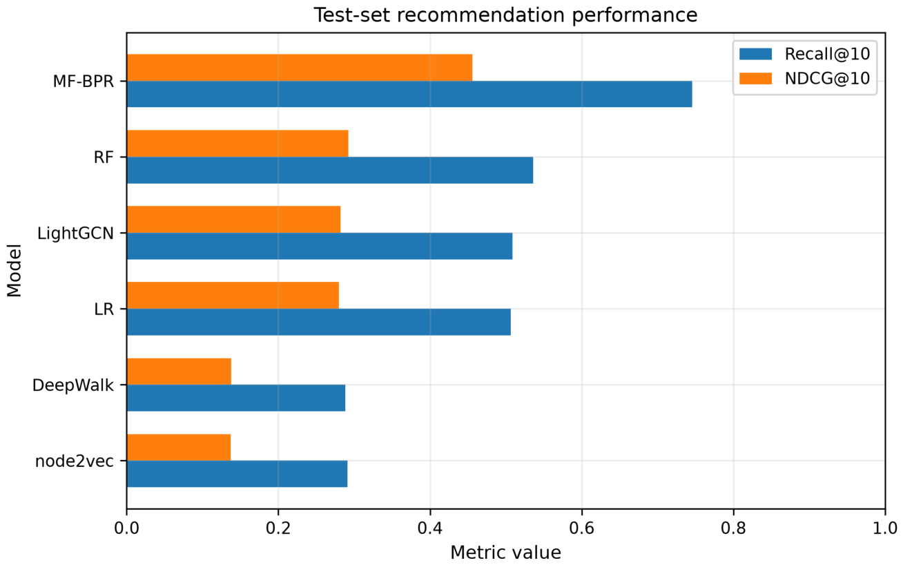
Figure 2.
NDCG@10 with 95% user-level bootstrap confidence intervals.
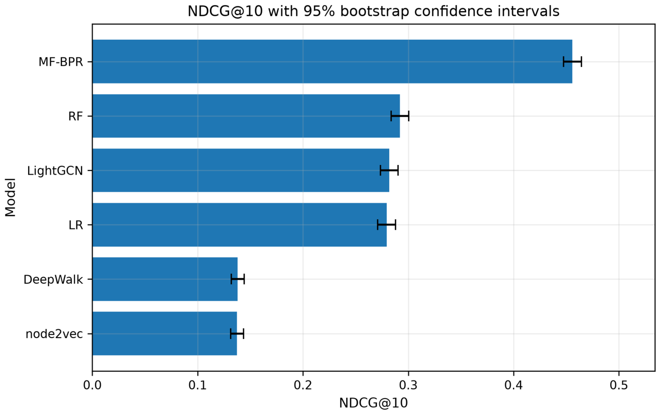
Figure 3.
Distribution of the rank assigned to the held-out positive movie.
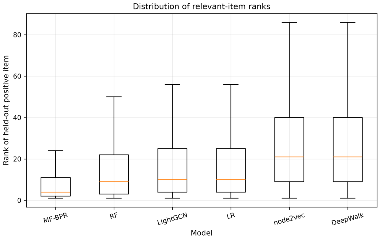
Figure 4.
Trade-off between test NDCG@10 and total training time.
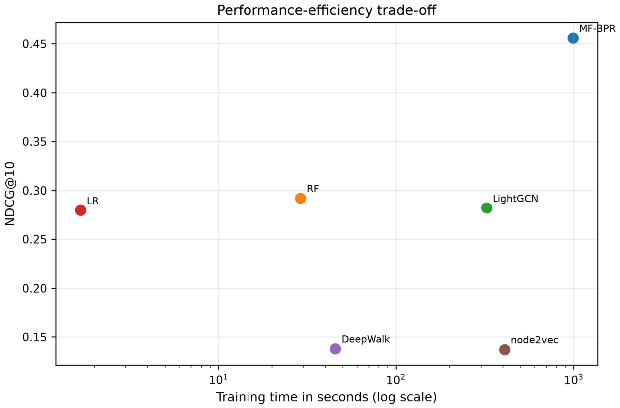
Figure 5.
NDCG@10 across quartiles of positive training activity.
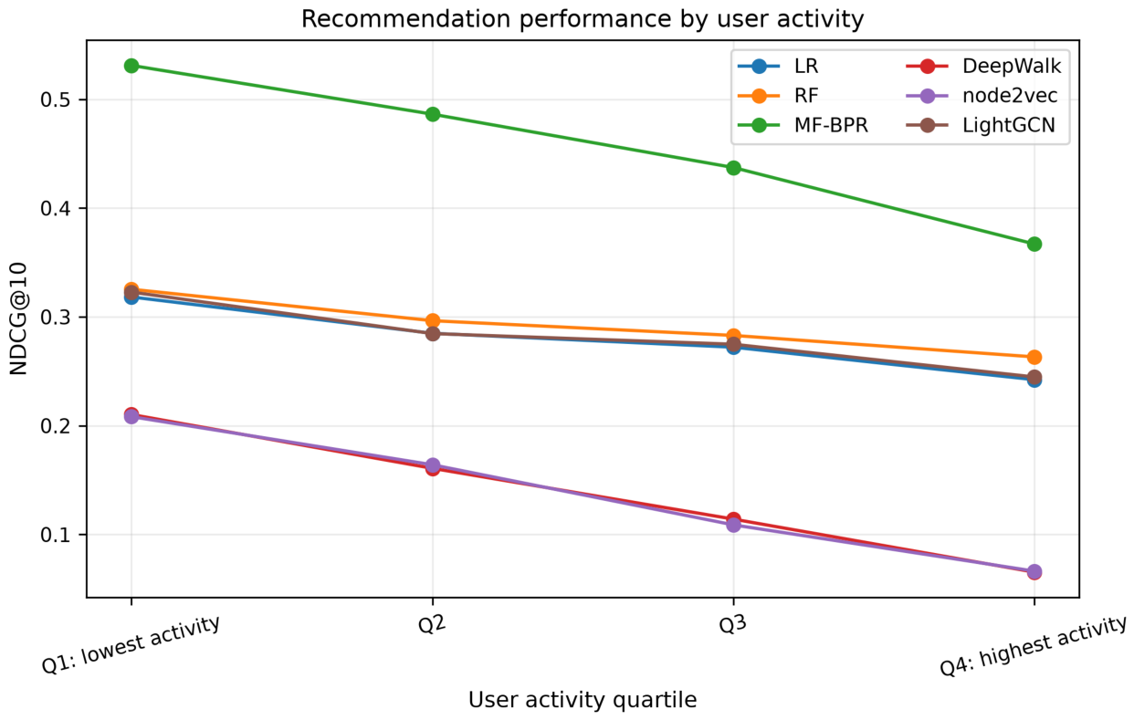
Figure 6.
NDCG@10 across quartiles of held-out movie popularity.
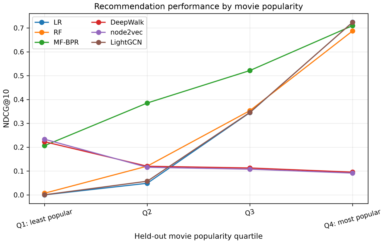

Table 1.
Top-K recommendation performance on the held-out test set.
| Model | R@5 | N@5 | R@10 | N@10 | R@20 | N@20 |
|---|---|---|---|---|---|---|
| Matrix Factorization BPR | 0.5737 | 0.3996 | 0.7458 | 0.4558 | 0.8896 | 0.4924 |
| Random Forest | 0.3629 | 0.2364 | 0.5362 | 0.2921 | 0.7261 | 0.3404 |
| LightGCN | 0.3473 | 0.2300 | 0.5085 | 0.2819 | 0.6984 | 0.3299 |
| Logistic Regression | 0.3403 | 0.2259 | 0.5062 | 0.2796 | 0.6948 | 0.3271 |
| DeepWalk | 0.1630 | 0.0977 | 0.2883 | 0.1380 | 0.4865 | 0.1877 |
| node2vec | 0.1596 | 0.0951 | 0.2910 | 0.1372 | 0.4915 | 0.1874 |
R: Recall; N: NDCG.
Table 2.
User-level bootstrap confidence intervals for the main test metrics.
| Model | Recall@10, 95% CI | NDCG@10, 95% CI |
|---|---|---|
| Matrix Factorization BPR | ||
| Random Forest | ||
| LightGCN | ||
| Logistic Regression | ||
| DeepWalk | ||
| node2vec |
Table 3.
Rank of the held-out positive item among 100 candidates.
| Model | Mean rank | Median rank | Mean reciprocal rank |
|---|---|---|---|
| Matrix Factorization BPR | 8.66 | 4 | 0.3793 |
| Random Forest | 15.56 | 9 | 0.2394 |
| LightGCN | 16.72 | 10 | 0.2350 |
| Logistic Regression | 16.78 | 10 | 0.2326 |
| node2vec | 26.72 | 21 | 0.1185 |
| DeepWalk | 26.79 | 21 | 0.1204 |
Table 4.
Predictive performance and computational cost.
| Model | Training time (s) | Test inference time (s) | NDCG@10 |
|---|---|---|---|
| Matrix Factorization BPR | 989.42 | 0.1046 | 0.4558 |
| Random Forest | 28.99 | 1.1024 | 0.2921 |
| LightGCN | 322.32 | 0.1144 | 0.2819 |
| Logistic Regression | 1.67 | 0.1350 | 0.2796 |
| DeepWalk | 45.45 | 0.1157 | 0.1380 |
| node2vec | 408.89 | 0.1184 | 0.1372 |
Disclaimer/Publisher’s Note: The statements, opinions and data contained in all publications are solely those of the individual author(s) and contributor(s) and not of MDPI and/or the editor(s). MDPI and/or the editor(s) disclaim responsibility for any injury to people or property resulting from any ideas, methods, instructions or products referred to in the content. |
© 2026 by the authors. Licensee MDPI, Basel, Switzerland. This article is an open access article distributed under the terms and conditions of the Creative Commons Attribution (CC BY) license (http://creativecommons.org/licenses/by/4.0/).
Copyright: This open access article is published under a Creative Commons CC BY 4.0 license, which permit the free download, distribution, and reuse, provided that the author and preprint are cited in any reuse.