

Submitted:
27 September 2026
Posted:
29 September 2026
You are already at the latest version
Abstract
A standing-wave closure condition in Delta-c Mechanics has two lowest exact orbital solutions: a closed full-orbit branch and an open half-orbit branch. These define, respectively, the atomic and nuclear kernels and satisfy the reciprocal relation α K_A K_N = 1. The principal result is the existence, within the proposed two-photon dynamics, of a single standing-wave closure condition whose two lowest branches correspond to the atomic and nuclear domains. The particle-mass relations that follow are presented as quantitative tests of this structural correspondence, not as an independent derivation of the mass spectrum; a unique, mass-independent generation rule for all higher harmonic assignments remains an open problem, stated as such in Appendix F. The reflecting interior boundary selects even Fourier modes and half-contour phase-lock conditions; multi-flow kernel products then determine rest-mass ratios through the binding law m_x/m_e = √E_x. The proton defines the three-flow nuclear ground state and is disclosed as the calibration identity for the anomalous nuclear ratio η. Independent tests include the neutron (0.268 ppm raw discrepancy), the charged pion (1.5σ from PDG 2024), the muon (−4.1 ppm raw), the tauon (within present uncertainty with a stated higher-harmonic prediction), and the top quark (within its 0.4 GeV measurement uncertainty). The purpose is not to replace QCD or electroweak theory in this paper, but to test whether one harmonic closure structure displays quantitative consilience from hydrogen spectroscopy to the nuclear mass scale.
Keywords:
standing-wave closure
; harmonic quantization
; atomic kernel
; nuclear kernel
; particle masses
; fine-structure constant
; two-photon electron
; probability-flow kernels
; neutron mass
; charged pion
1. Introduction
1.1. Central Claim
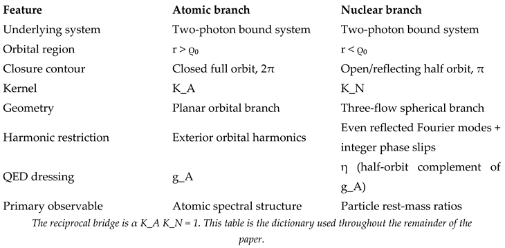
The principal claim of this paper is structural rather than numerical: the atomic and nuclear domains are proposed to be two harmonic branches of one standing-wave closure condition. The same two-photon bound system is used on both sides of the electron creation radius. Outside that radius the stable solution is a closed full orbit; inside it the reflecting boundary admits an open half-orbit solution. The resulting kernels are therefore not independently chosen atomic and nuclear rules, but two solutions of one closure problem.
Delta-c Mechanics [1,2] models the electron as two photons in mutual circular orbit at the Compton scale. The pair has an orbital radius, orbital frequency, and probability-flow density. Stable orbital states are indexed harmonically. Each stable state defines a Vertex Kernel, and simultaneous occupation of several kernel states defines a Vertex Function. Rest-mass ratios are then calculated from the joint kernel product through the binding law developed below.
The key test is whether the harmonic order is fixed before the particle mass is evaluated. In the atomic branch the harmonic structure has already been applied to hydrogen fine structure [18]. In the nuclear branch the allowed powers arise from the same phase-lock condition together with the reflecting interior boundary. The paper therefore presents the closure condition and harmonic selection rule before the particle calculations, so that the numerical comparisons can be read as tests of a prior construction rather than as the source of that construction.
The strongest numerical claims are separated from calibration and from open problems. The proton supplies the disclosed calibration identity for η and fixes the three-flow nuclear ground state. The neutron, charged pion, muon, tauon, and top quark provide increasingly independent tests. The neutral-pion interpretation, neutrino structure, and detailed electroweak W/Z discussion are not needed for the argument developed here and are deferred to companion work.
1.2. Scope and Standard of Test
This paper asks a limited quantitative question: does the common closure construction generate the observed mass hierarchy to the stated precision? The harmonic assignments used are fixed by the framework’s stated constraints; whether those constraints select the assignments uniquely, with the measured masses absent from the selection, is established here for the proton through its three-flow geometry and posed as an open problem for the heavier states (Appendix F). Questions concerning a complete Lagrangian formulation, gauge structure, confinement, and parton distributions remain open and are not treated as solved here. Appendix H records those limitations explicitly.
Accordingly, the evidential order used here is: (i) establish the common standing-wave closure; (ii) identify its atomic and nuclear branches; (iii) derive the reflecting-boundary harmonic rule; (iv) state the mass law and the three-flow proton geometry; and only then (v) compare calculated masses with CODATA and PDG values. This order is intended to make the origin of the harmonics auditable by a skeptical reader.
1.3. Relation to Prior Composite-Particle Proposals
The two ideas underlying this paper, the electron as a Compton-scale circulation of light, and heavier particles as composites of electron-like constituents, both have serious precedents, and the paper’s claim of novelty is placed against them explicitly. Barut [3,4] built the leptons and hadrons from stable electromagnetically-bound leptons and obtained the celebrated formula ; the present framework reaches 206.767 (−4.1 ppm raw) by a different mechanism, orbital kernel states rather than magnetic self-binding, and extends the same machinery to the baryons. Hestenes’ zitterbewegung interpretation [5] places a Compton-scale circulation at the heart of the electron with spin as its orbital angular momentum and from the circulation; the present two-photon electron shares that kinematic core while replacing the circulating point charge with a bound photon pair and removing charge as a primitive. Williamson and van der Mark [6] proposed the electron as a photon confined on a toroidal path, the closest structural ancestor of the two-photon closure. On the composite side, the preon models of Harari and Shupe [7,8] built quarks and leptons from three sub-constituents, anticipating the three-constituent baryon; they required new fractionally-charged fundamentals and met the composite-mass paradox, a bound state far lighter than its binding scale [9], which the present framework avoids structurally: constituent masses do not add, the bound mass is a deficit energy assembled by the product rule (Appendix B), so no cancellation between large constituent masses and large binding is needed. What distinguishes the present work from all of these precedents is not the ideas but the arithmetic: a parameter-free spectrum at the precisions of Section 8, with its one calibration disclosed; Appendix G establishes that the framework-derived value of that calibrated constant reproduces the proton mass to 13.6 parts per billion before calibration.
The quantitative summary is given in Section 8. The central independent comparisons retained in the main text are the neutron, charged pion, muon, tauon, and top quark. The proton is presented separately as the ground-state calibration identity, not counted as an independent precision prediction.
2. The Common Standing-Wave Closure Condition
The atomic-nuclear connection is stated first because it supplies the organizing principle for every later mass formula. The two-photon electron consists of photons A and B counter-propagating on the same orbit. Their combined probability-flow density forms a standing wave. Self-consistent states occur when the accumulated phase perturbation closes over the traversal interval.
Because the closure factor vanishes for every integer harmonic at the allowed traversal angles, the condition is satisfied simultaneously at all orders rather than as a single fitted approximation. The two lowest solutions are the open half orbit (nuclear kernel) and the closed full orbit (atomic kernel). Thus the two domains are generated by one condition rather than introduced as separate structures.
Figure 1.
Atomic and nuclear branches of the same standing-wave closure condition. The closed full orbit (Δθ = 2π) defines the atomic kernel K_A and the open half orbit (Δθ = π) defines the nuclear kernel K_N. The branches satisfy α K_A K_N = 1. This reciprocal relation is the bridge developed through the remainder of the paper.
Figure 1.
Atomic and nuclear branches of the same standing-wave closure condition. The closed full orbit (Δθ = 2π) defines the atomic kernel K_A and the open half orbit (Δθ = π) defines the nuclear kernel K_N. The branches satisfy α K_A K_N = 1. This reciprocal relation is the bridge developed through the remainder of the paper.
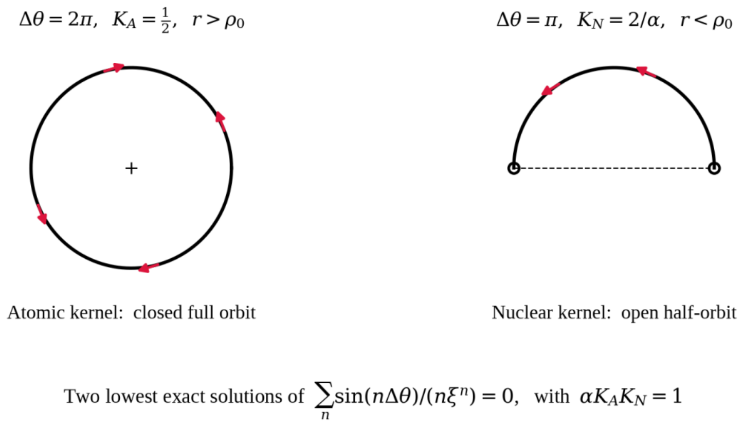
The full-orbit and half-orbit contours also relate the two anomalous delay factors. Time-reversal symmetry of the counter-propagating pair makes the relevant coupling density even in the orbital angle, so the half-orbit contribution is one half of the corresponding full-orbit contribution at each loop order. The detailed all-orders argument is retained in Appendix E.5.
The result is used here only as the branch relation needed to organize the harmonic construction. The absolute QED coefficients are taken from the established electron anomaly; their Delta-c interpretation is developed in Appendix C, Appendix E and Appendix G.
3. The Two Branches of the Two-Photon Orbital System
3.1. The Electron Creation Radius
Delta-c Mechanics postulates the photon as a rotating Planck particle with probability flow rotating at the Compton frequency. The change in the local speed of light at distance from such a particle defines the elemental Vertex Kernel. It is simultaneously the probability amplitude that the photon’s flow passes through an interaction region of size , and the fractional reduction in local light speed that constitutes the binding mechanism.
Two photons in mutual orbit bind when each reduces the other’s propagation speed sufficiently to redirect it into a closed path. The radius of that closed path is the electron creation radius. A result verified to ten significant figures is:
where cm is the classical electron radius. The QED loop corrections that modify the gyromagnetic ratio modify the effective orbital radius of the bound photon pair in the same proportion. The creation radius is the classical electron radius corrected by the full anomalous g-factor.
3.2. Atomic and Nuclear Kernel States
The two-photon bound system admits a spectrum of stable orbital states where the angular momentum of the orbiting photons is an integer multiple of . The Atomic Kernel applies when . At these larger radii the QED rotational delay through increases the effective radius:
The Nuclear Kernel applies when . At these smaller radii the Anomalous Nuclear Ratio governs the adjustment (Section 7 and Appendix G):
These two kernels differ in magnitude by the square of their ratio. The ratio of approximately 75,000 is the fundamental reason nuclear particle masses are so much larger than atomic energy scales. It arises entirely from the scale ratio , not from any additional assumptions.
3.3. The Central Scale Ratio
The ratio of the electron Compton wavelength to the creation radius:
is the central dimensionless parameter of the entire framework. Every kernel amplitude is a power of .
4. Atomic Branch and Prior Spectroscopic Test
The atomic branch is not introduced in this paper to assist the nuclear fit. In the companion hydrogen fine-structure work [18], the exterior closed-orbit kernel is applied to hydrogen spectral structure. The present paper uses that atomic result as the independently developed side of the same closure construction. The nuclear branch begins only after the creation-radius boundary changes the allowed contour from the full orbit to the reflecting half orbit.
The significance of the bridge is therefore one of consilience: the same fine-structure constant and the same anomalous electron factor enter both branches, while the branch change is geometric. Atomic spectroscopy and nuclear rest masses are treated as distinct observables generated by one harmonic closure system, not as two independently parameterized sectors.
5. Harmonic Generation at the Reflecting Boundary
The origin of the nuclear harmonic powers must be fixed before the particle masses are calculated. Inside the creation radius the paths reflect at the boundary. Reflection makes the secular flow amplitude even, so only even Fourier modes survive the orbit average. The averaging contour is a half period (out and back), which supplies the universal half-contour normalization relative to the exterior full-orbit branch.
The Planck and orbital frequencies are phase locked at the creation radius. Additional interior kernel states permit the lock to slip only by integer phase increments. Each allowed slip contributes a discrete harmonic factor to the kernel amplitude. The admissible set for a particle is constrained jointly by closure of the total vertex exponent, continuity of root-paired factors, and the normalization imposed by the reflecting half-contour. Bare power counting by itself admits many formal combinations and is therefore not used as the selection rule.
For the proton ground state, spherical symmetry requires three simultaneous orthogonal nuclear flows. The closure set retained by the bounded Fourier construction is the minimal three-flow set consistent with the exact proton vertex exponent. For the muon, two effective nuclear flows give the lowest even two-flow closure. The full algebraic enumeration and the historical alternatives are retained in Appendix F; only the selection principle required to audit the main calculations is used here.
6. From Kernel Products to Rest Mass
6.1. Ground-State Energy
The binding of two electrons at the creation radius , accounting for the QED rotational delay through , defines the reference energy:
is a dimensionless ratio of the ground-state orbital energy to the electron rest energy. It contains no adjustable parameters. Numerically .
6.2. Binding Mass Formula
The mass of any bound configuration relative to the electron mass is:
where is the Vertex Function, the product of all kernel amplitudes entering the configuration. The square root arises from the virial theorem: at equilibrium in a stable bound state, kinetic and potential energies are equal, giving a square-root relationship between interaction energy and the resulting mass.
The square root is not an imported theorem; it follows from two results established elsewhere in this paper. First, for an orbital standing wave, rest mass is frequency content, , the mass–frequency identity of Appendix E.4, verified there against the harmonic dictionary at three orders. Second, the Vertex Function is a product of flow amplitudes (Section 6.3), and the energy density of a standing wave is quadratic in its amplitude, so the vertex energy is the squared quantity while the frequency, and therefore the mass, is its square root. The virial equilibrium fixes only the numerical factor in the ground-state energy (Appendix H); the square-root lawform itself is forced by the amplitude-to-energy relation. Stated as bookkeeping: vertex energies compose linearly in , masses compose in quadrature, which is why the neutron relation is exact addition in the space where the lawform lives.
6.3. Why the Vertex Function Is a Product
At the Compton scale the Vertex Kernel is the probability amplitude that the photon flow occupies an interaction region of size . For two kernels and at a vertex, the probability that both flows simultaneously occupy their characteristic radii is, by the product rule for independent events, . Given the framework assumption that the kernel occupations are independently established by their respective closure conditions, their simultaneous occupation is represented by the standard product rule for independent probabilities.
The orbital state of each kernel is determined independently by the standing-wave closure condition before interaction. A vertex forms only when these independently established kernel states are simultaneously occupied. Their joint occupation therefore follows the ordinary product rule for independent events.
6.4. Three-Flow Nuclear Ground State
The proton vertex requires three nuclear kernel insertions. The derivation follows from the change in orbital topology at the creation radius:
- For (atomic domain): planar orbital symmetry. Two independent projection axes are available → Atomic Kernel product .
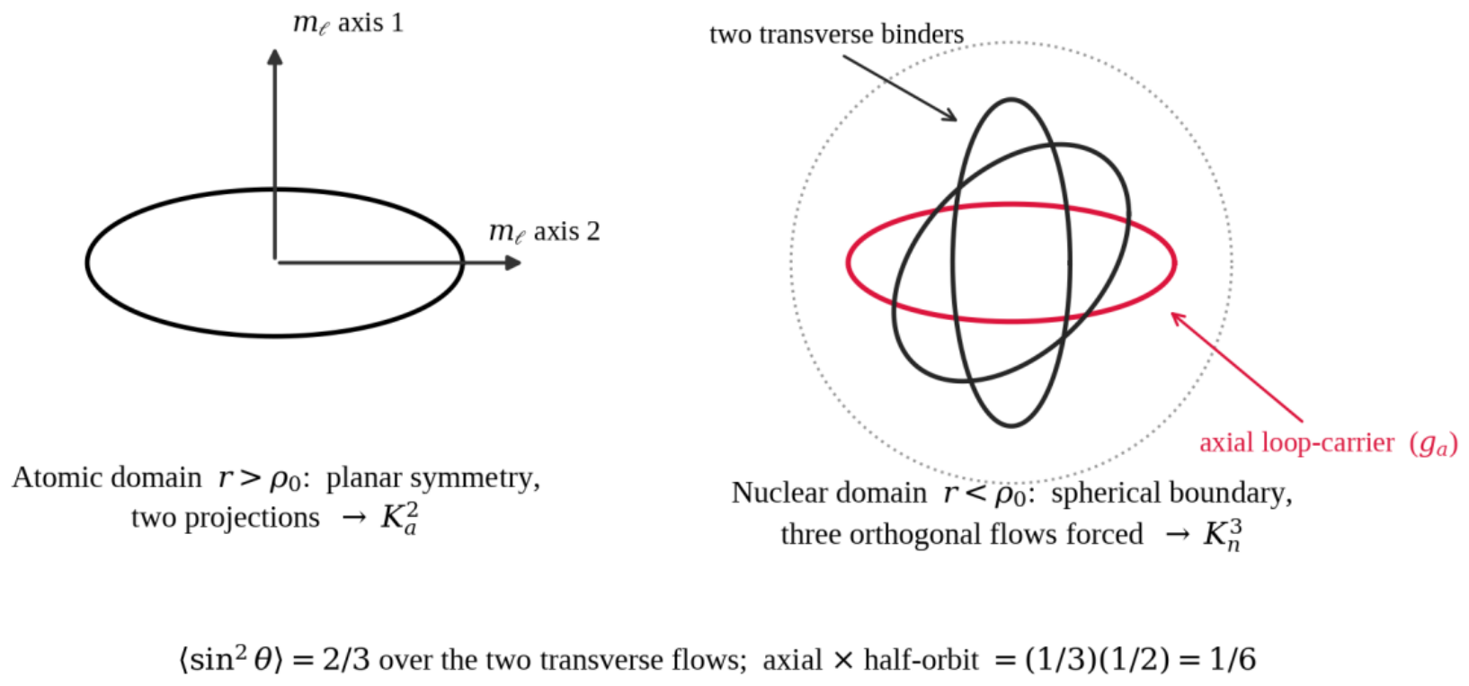
- For (nuclear domain): full spherical symmetry. Three orthogonal projections must be simultaneously occupied to satisfy the boundary condition at . The ground state saturates all three projections (analogous to Hund’s rule) → Nuclear Kernel product as the minimal nuclear unit.
This geometric argument forces for the proton. As a consistency check, the resulting integer (odd) correctly predicts fermion statistics independently, confirming the geometric derivation is internally consistent rather than requiring the spin-statistics result to justify the structure.
Figure 2.
Change in orbital topology at the creation radius. The exterior atomic branch is planar, while the interior nuclear branch requires three orthogonal flows. The proton ground state saturates the three-flow nuclear geometry; one flow is axial and two are transverse.
Figure 2.
Change in orbital topology at the creation radius. The exterior atomic branch is planar, while the interior nuclear branch requires three orthogonal flows. The proton ground state saturates the three-flow nuclear geometry; one flow is axial and two are transverse.
7. QED Dressing Factors
Two anomalous factors enter the numerical implementation. The measured electron gyromagnetic anomaly g_A characterizes the closed-loop exterior delay. Its nuclear counterpart η is associated with the open half-orbit standing-wave insertion. The leading half-orbit relation follows from the common closure geometry; the small residual required for the proton ground state is analyzed as internal orbital energy in Appendix G. The proton is therefore treated as the disclosed calibration identity for η in the main numerical table, while Appendix G separately tests how closely η can be reconstructed from g_A and the independently defined ground-state energy.
This separation is important for interpreting precision. Agreement of the proton with CODATA is not counted as an independent eleven-digit prediction in the evidential summary. The neutron, pion, muon, tauon, and top calculations are the relevant tests of whether the harmonic structure propagates beyond the calibration state.
8. Mass Calculations and Tests
8.1. Representative Calculations
Proton, 1836.15267343 mₑ (CODATA: 1836.15267343)
Three nuclear kernels and the virial factor represent the three-flow orbital geometry of the proton, derived in Section 6.4; Equation (8) with Equation (6) reduces to the exact closed form shown row by row below (factors displayed rounded; the closed form is exact):
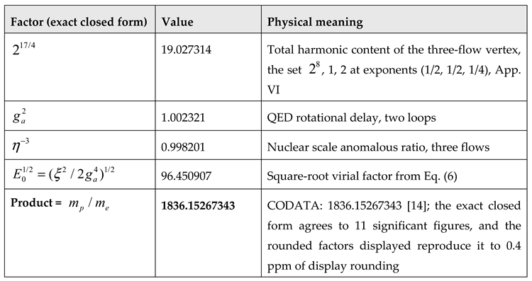
Equations (9) and (4) reduce to the exact proton closed form shown in the table above. In this paper that equality is used as the calibration identity fixing η for the nuclear ground state. Appendix G then asks the separate question of how far η can be derived from g_A and the internal orbital energy without using the proton mass.
Neutron, 1838.68415 mₑ (CODATA: 1838.68366173, 0.268 ppm)
The neutron formula follows from the vertex function structure: the neutron carries the proton vertex energy plus one electron bound at the nuclear ground state :
The raw neutron calculation differs from CODATA by 0.268 ppm. This raw value is the principal comparison in the main text. Appendix D examines the residual and shows that its magnitude is of one-loop order with a geometric suppression close to 1/6; the corrected value is reported separately rather than used to define the harmonic state. An exact regrouping relating the neutron binding term to the charged-pion kernel provides an independent control on the localization of that correction; see Appendix D.4.
Muon, 206.76743476 mₑ (exp: 206.76828298, −4.1 ppm)
The raw muon vertex is low by 4.1 ppm. Appendix D compares that residual with the known two-loop anomalous-moment scale and reports the corrected value separately. The harmonic assignment itself is not altered by the correction.
Tauon, 3477.18825 mₑ (exp: 3477.135 ± 0.136)
The tauon vertex lies within the present experimental uncertainty. The framework also states a higher-harmonic value of 3477.2269 m_e as a prospective test. The purpose of retaining that number is falsifiability: improved tau-mass measurements can distinguish the proposed harmonic continuation from the present vertex value.
Charged Pion, 273.131906 mₑ (PDG 2024: 273.13244 ± 0.00035 mₑ, 1.5σ)
The charged-pion calculation is 1.95 ppm below the PDG 2024 value, corresponding to 1.5σ of the quoted measurement uncertainty. No residual correction is introduced. This case is therefore a useful independent scale test of the nuclear kernel construction.
Top Quark, 171.774 GeV (PDG: 171.77 ± 0.38 GeV)
The top vertex closed form is
The calculated top-quark value lies within the 0.38 GeV experimental uncertainty. The 25 ppm proximity to the central value is noted but is not counted as a precision test, since the measurement itself is precise only to about 2200 ppm; the case provides a high-mass structural check using the explicit heavy-sector vertex construction, and the full kernel factorization is retained in Appendix F.
8.2. Summary of Quantitative Tests
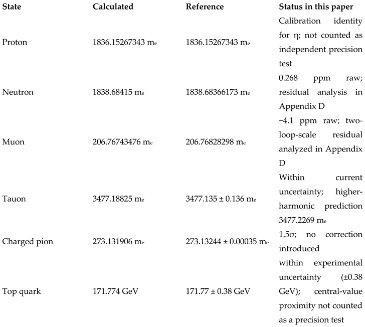
The evidential hierarchy is deliberate. The proton fixes the nuclear ground-state calibration. The neutron and charged pion are the cleanest light-sector tests because their raw discrepancies can be stated without changing the harmonic assignments. The muon and tauon test the lepton branch, and the top quark tests continuation to the heavy sector. Detailed residual corrections are supplementary to, not generators of, the harmonic states.
9. Consilience Across the Creation Boundary
The significance of the construction is not any single mass agreement but the continuation of one harmonic architecture across two experimentally distinct domains. In the exterior branch, the closed-orbit kernel is used in hydrogen fine-structure calculations [18]. At the creation radius the boundary condition changes, but the standing-wave closure principle does not. The interior branch then generates the nuclear kernel and the particle-mass hierarchy.
Both branches are controlled by the same fine-structure constant and the same electron anomalous factor, with η introduced as the half-orbit nuclear complement. The nuclear kernel scale lies naturally near the charged-pion mass, while the full vertex construction refines the pion comparison to 1.5σ. This cross-domain continuity is the central consilience claim of the paper and the reason the atomic branch is presented before the nuclear mass table.
10. Conclusions
The framework remains incomplete. This paper does not derive QCD confinement, electroweak gauge structure, or a complete field-theoretic formulation, and the detailed origin of some residual corrections remains open. Those limitations do not decide the narrower question tested here: whether a harmonic structure developed in the atomic branch can continue through the creation-radius boundary and generate a quantitatively organized nuclear mass spectrum. The calculations reported here are intended as tests of that specific claim.
With the harmonic structure fixed, the neutron, charged pion, muon, tauon, and top quark provide the main numerical tests. The neutron differs from CODATA by 0.268 ppm before the residual analysis; the charged pion lies 1.5σ from the PDG 2024 value without an added correction; the muon differs by 4.1 ppm raw; the tauon lies within present uncertainty and carries a stated higher-harmonic prediction; and the top-quark result lies within the quoted experimental uncertainty.
The reflecting interior boundary restricts the nuclear branch to even Fourier content and integer phase slips. Multi-flow topology then determines the allowed kernel products. For the proton ground state the nuclear geometry requires three orthogonal flows; the proton itself is used as the disclosed calibration identity for η rather than as an independent precision prediction.
This paper is organized around one proposition: atomic and nuclear structure are two harmonic branches of the same standing-wave closure condition. The closed full-orbit solution defines the atomic kernel, the open reflecting half-orbit solution defines the nuclear kernel, and the two are linked by the reciprocal relation α K_A K_N = 1.
Supplementary Materials
The following supporting information can be downloaded at the website of this paper posted on Preprints.org, Supplementary File S1: numerical verification worksheet reproducing the mass calculations of Section 8 from the two inputs.
Funding
This research received no external funding.
Data Availability Statement
No new data were created or analyzed in this study; all numerical comparison values are the published CODATA and Particle Data Group values cited in the text. Data sharing is not applicable to this article.
Conflicts of Interest
The author declares no conflict of interest.
Appendix A. Physical Constants
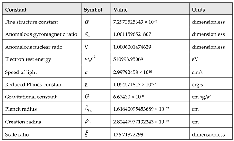
Appendix B. Eddington’s Multiplicative Hypothesis
In his 1936 lectures Arthur Eddington [20] observed that the wavefunction of two independent particles at positions and is exactly . This product form is not an approximation, it is exact for independent particles. Eddington conjectured that mass might arise from the same multiplicative structure of wavefunctions. Delta-c Mechanics provides the mechanism: the Vertex Kernel is the analogue of at the interaction scale, and the joint occupation probability of independent flows is their product. The Vertex Function is multiplicative for the same reason the two-particle wavefunction is multiplicative: independent amplitudes multiply.
Appendix C. Photon-Flow Derivation of
Section 2 derives from the standing-wave closure condition and the time-reversal symmetry of the two-photon system. This appendix presents a complementary derivation from the photon-flow counting rules, confirming that the topological and mechanical pictures describe the same physics.
Appendix C.1. The Atomic Kernel and the Origin of
In the two-photon electron the Atomic Kernel governs orbital states with . At these radii the two photon flows are symmetric: one axial () and one transverse (). The axial flow has a non-zero probability of executing a virtual closed loop, temporarily absent from the creation radius. The full Schwinger series for this closed-loop delay gives . The transverse flow carries no closed-loop delay. The effective action ratio is the mean over the two flows: one flow contributes , one contributes 1, giving mean .
Appendix C.2. The Nuclear Kernel and the Origin of
The Nuclear Kernel governs orbital states with . At sub-Compton radii the spherically symmetric core produces three mutually orthogonal photon flows. Of the three, only one is axial (experiencing the closed-loop delay); the other two are transverse (no delay). The axial flow traverses the open half-orbit rather than the closed full orbit, carrying the closed-loop delay at half order, the square root of the full delay factor:
Since is within 0.12% of unity, and agree to within 0.17 ppm. The leading formula is identical to the result obtained from the standing-wave closure condition and from the exact all-orders proof. The three routes converge because they describe the same physical process: one of the three nuclear flows executing a half-loop rather than a full loop.
Appendix C.3. Numerical Verification
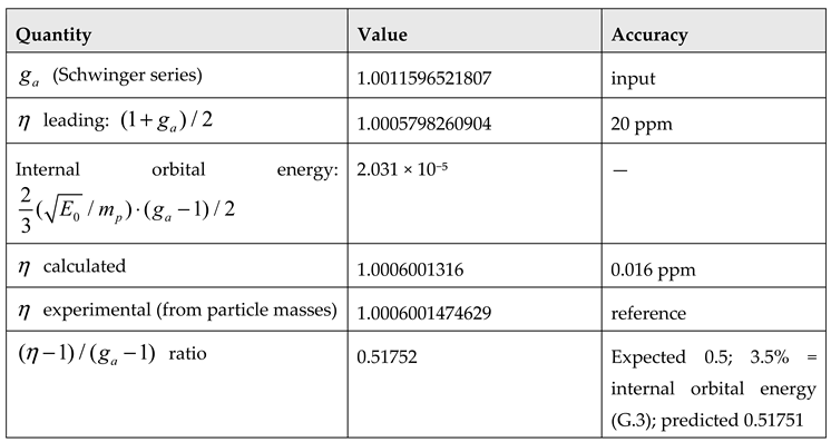
The ratio departs from the exact value 0.5 by 3.5%. This residual is the proton’s internal ground-state orbital energy distributed over the three nuclear flows, (G.3), giving 0.51751 against the measured 0.51752. It is not the two-loop Källén–Sabry term, which is a factor of about two too small. The two converging derivations of the leading term (closure-condition proof and flow counting), together with the internal-orbital-energy residual, give a parameter-free determination of from and .
Appendix D. The 0.268 ppm Neutron Residual and the QED Correction to
The formula reproduces the CODATA neutron mass to 0.268 ppm. The discrepancy is real, it exceeds the CODATA measurement uncertainty (±0.00064 ppm) by approximately 400 standard deviations, but it is physically identified and of a known class.
Appendix D.1. The Residual on
The exact value of required to reproduce exactly is:
The formula gives , which is 194.6 ppm too large. The fractional mass error is suppressed by the factor , giving exactly 0.268 ppm on the mass.
Appendix D.2. Scale Analysis and Physical Origin
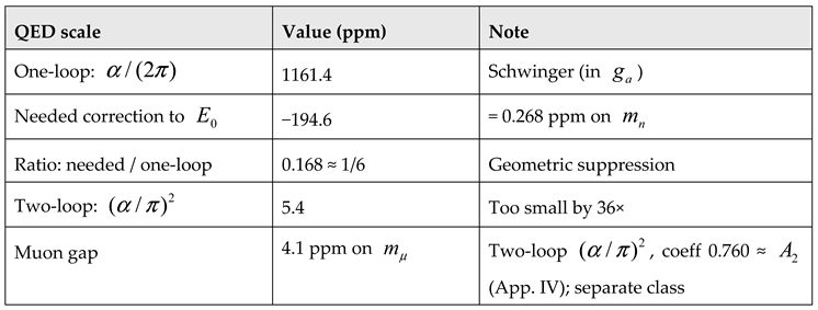
The ratio 194.6/1161.4 = 0.168 ≈ 1/6 shows the correction is of one-loop magnitude with a geometric suppression of approximately 1/6. The two-loop scale (5.4 ppm) is 36 times too small, confirming it is a one-loop effect with a suppressed coefficient.
Appendix D.3. Status
The muon and neutron residuals are different classes, not structurally identical. The muon gap (−4.1 ppm) sits at the two-loop scale ppm with an order-one coefficient (), a genuine second-order QED correction to the muon vertex. The neutron gap (0.268 ppm) is a one-loop correction to suppressed by a geometric factor . The residual is neither, it is the internal-orbital-energy effect of G.3. Each is an identified next calculation of its own class. The corrected neutron formula is:
where the coefficient 1/12 is derived from the flow assignment already fixed in G.3: the one-loop correction acts on the axial flow only, the loop-carrier, one of the three orthogonal flows, and on the open half-orbit contour, giving suppression on , i.e., ppm against the required 194.6 ppm on ; the 1.0 ppm remainder (≈ +0.0013 ppm on , about 2σ of the CODATA uncertainty) is second-order. Scope: this correction applies to in its neutron-channel role as the binding energy of the added pair. It does not apply to as the proton’s internal virial factor, a universal application would shift the proton mass by −97 ppm and is excluded; the two roles are physically distinct (interaction energy of an added pair versus the internal ground-state virial of the proton’s own three flows).
Appendix D.4. Localization via the Regrouping Identity
Equation (6) admits an exact regrouping. With , ; using and , , so
Thus the neutron binding term and the charged-pion vertex share the exact algebraic core , but with different dressings: in the neutron binding term and in the charged-pion vertex. This is an algebraic regrouping of the existing expressions and introduces no new parameter or numerical adjustment; the neutron prediction and its +0.268 ppm residual are unchanged. Attempts to represent the neutron as containing two complete pion vertices fail under both additive and multiplicative composition and are rejected; the exact surviving relation is the common factor . A bookkeeping consequence: contains no power of , so every in the neutron mass formula enters through the proton-side construction. Whether the dressing exchange reflects a deeper combinatorial rule remains open. The localization of the Appendix D one-loop correction that this regrouping enables, with the charged pion as external control, is developed below.
The regrouping identity above, with the charged-pion vertex , permits the correction of Equation (D2) to be localized within the factors of , and supplies an external measured control that the scope argument of D.3 lacks.
The pion control. The correction of Equation (D2) multiplies ; within the factorization it could a priori attach (i) universally to the shared core wherever that core occurs, (ii) to the core only in its role, or (iii) to the atomic dressing . Hypothesis (i) is excluded by measurement: a universal core correction would shift the charged pion by ppm, while the calculated pion agrees with the PDG value at ppm (), exclusion by two orders of magnitude, and the external, measured counterpart of the internal proton-virial exclusion of D.3. Hypotheses (ii) and (iii) are numerically indistinguishable within the neutron, since both multiply by the same factor; what selects (iii) is the flow derivation of D.3, in which the selects the loop-carrier flow, an atomic-side object, and what would discriminate between them independently is the insertion rule below, wherever a dressing recurs. The pion’s own freedom from the correction is consistent under (iii): its dressing is , and carries its QED structure by construction.
Kernel restatement of the 1/6. The flow assignment of D.3, the loop-carrier axial flow, one of three, taken on the open half-orbit contour, reads in the regrouped language as one Schwinger insertion on the atomic dressing: , with the half-orbit factor and the per-flow selection. The identity is exact; it attaches the derived suppression to the same objects that carry ’s kernel form, so the flow-language and kernel-language accounts of the 1/6 are one statement.
The second-order remainder, quantified. After Equation (D2) the uncovered fraction of is , an order-one coefficient at the two-loop scale, consistent with the classification in D.3 of the ppm as second-order (about of the CODATA uncertainty, ppm). The coefficient 0.720 in units is the named target for the two-insertion counting on ; no closed form is claimed here.
on carries the one-loop insertion with multiplicity governed by and the flow selection, while bare-core quantities carry none. The charged pion is the first passed control ( on the core side); the rule becomes falsifiable wherever another structure occurs in the framework. Until such an occurrence is identified, the assignment to rests on the flow derivation of D.3 together with the measured exclusion of hypothesis (i); the localization claimed here is exactly that much, and no more.
Appendix E. Derivation of from Orbital Photon Flow Density
This appendix presents the flow-density derivation of from within Delta-c Mechanics. The leading Schwinger term is reproduced from first principles using the action-angle averaging theorem of classical mechanics. The value of used in the main paper is taken from QED; this appendix establishes the mechanical picture.
Appendix E.1. Setup
The free electron’s photons orbit at the creation radius , smaller than the reduced Compton wavelength by the factor . Photon A’s orbit is modified by photon B’s probability flow density at , not by B’s electromagnetic field. The relevant coupling is the ratio .
Appendix E.2. The Standing Wave
Photons A and B counter-propagate on the same orbit. Their combined flow density is . This standing wave is not an external perturbation, it is the unavoidable geometric consequence of two counter-propagating photons on the same orbit.
Appendix E.3. The Schwinger Result from the Averaging Theorem
The action-angle averaging theorem gives the secular frequency shift from the standing wave. With (so exactly):
Since : [Schwinger ✓]. The factor is not assumed, it comes from averaging over one complete orbit.
Appendix E.4. Feynman Loops as Fourier Harmonics
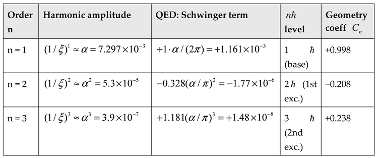
Each Feynman loop order corresponds to the th Fourier harmonic of the standing wave, coupling to the orbital action level. The alternating signs of reflect the orbit alternately compressing and expanding at each order. The correspondence is exact: rewriting the QED series in the orbit-average form requires , which reproduces the tabulated coefficients at all three orders (1.000, −0.209, +0.239 against 0.998, −0.208, 0.238, the first differing only by the dressing). The dictionary is therefore a theorem, not an empirical table, and it grounds the mass–frequency identity used in Section 6.2: for a standing wave , so the mass correction and the moment carry the same harmonic coefficients.
Appendix E.5. What Is Established
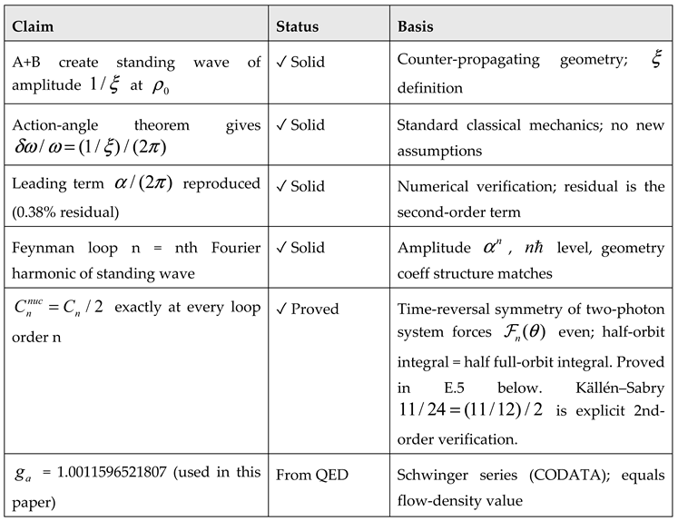
The entry for has been upgraded from ‘Open’ (v6f/v7) to ‘Proved’ in this version. The proof, given here in full (and archived in [11]), proceeds as follows: (i) the standing-wave closure condition is satisfied exactly at for all orders in because for every integer ; (ii) the time-reversal symmetry of the two-photon system (A and B are indistinguishable, so time reversal maps the system to itself exactly) forces to be even in at every loop order; (iii) even symmetry of forces exactly, giving for all . The Källén–Sabry coefficient is the explicit second-order verification. The open item that remains is computing the individual values from the full relativistic spin-1 orbital integral, which is precisely the QED loop integral in orbital language. Their halving on the nuclear contour is proved; their absolute values are not.
Connection to Appendix C
Appendix C derives from the half-orbit open insertion: . In the standing wave picture, the half-orbit traverses exactly half the modulation cycle, reducing the action-angle integral from to . The same standing wave drives both and ; the factor of 1/2 is the ratio of contour lengths and , proved exact to all orders by the closure condition and even-symmetry theorem [11].
Appendix F. Nuclear Kernels: Mechanical Picture, Harmonic Powers, and the Origin of Combined Mechanical Summary and Expanded Appendix
Introduction and Scope
This appendix presents the mechanical core of the nuclear particle mass calculations in Delta-c Mechanics. Particle masses arise as products (under a virial square-root) of internal vertex kernels. The kernels themselves are generated by phase-locked two-photon binding, with integer phase-slip harmonics required by the reflecting boundary at the creation radius. The anomalous nuclear ratio is the bounded-interior counterpart to the anomalous gyromagnetic ratio . All results use only the independently measured constants and , plus the nuclear ratio , leading term fixed by , 3.5% residual from the independently-defined ground-state energy , the residual’s projection coupling being the transverse weight 2/3, forced by the flow assignment of the leading term and confirmed by the data.
Summary Table
Particle Masses from Photon-Flow Vertex Kernels
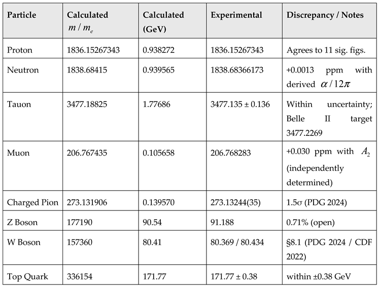
All calculations use only and , together with the nuclear ratio , whose leading term is fixed by (hence ) and whose 3.5% residual is the internal ground-state orbital energy of G.3, computed independently of the proton. The residual’s projection coupling is the transverse weight 2/3, forced by the flow assignment of the leading term and confirmed by the data. The identified muon and neutron residuals close to +0.030 ppm and +0.0013 ppm respectively via independently determined QED coefficients, at second order for the muon, and the derived axial-flow half-orbit coefficient at first order for the neutron (Appendix D).
Mechanical Derivation of the Harmonic Powers from the Bounded Fourier Model
A bookkeeping identity underlies the heavy-sector closed forms: the Planck-radius–cycle-number product satisfies to 1 part in 1012, so the kernel base equals exactly; this is what collapses the W, Z, and top kernel products of Section 8.1 to closed forms in ξ and η.
The integer powers appearing in the vertex functions (e.g., , , 2, …) are the minimal even integers that satisfy phase-lock closure for a given multi-flow topology when paths reflect at .
In the two-photon binding picture the Planck and orbital frequencies are phase-locked at the creation radius. Additional kernels inside that radius allow the lock to slip by integer multiples of . Each slipped quantum contributes a factor
to the kernel amplitude.
Inside the creation radius the paths reflect at the hard wall . The reflecting boundary forces every flow amplitude to be even under reflection. Only even Fourier modes of the central standing wave survive in the secular average, and the averaging contour is a half-period (out-and-back). This even-symmetry projection plus half-contour normalization supplies the universal factor 1/2 relative to the free exterior case.
The proton ground state requires three simultaneous orthogonal nuclear-kernel insertions to satisfy spherical symmetry inside ( structure). The harmonic set that closes all three phase locks after reflection is , 1, 2 with factor exponents , giving total harmonic content , exactly the vertex exponent required by the closed form of §8.1, with the quarter exponent on the third factor matching the exact constituent ratio of the companion structure analysis. (An earlier statement of this set as n = 6, 2, 2 is withdrawn: enumeration shows it cannot reproduce the exact vertex exponent under any tested exponent assignment.)
The muon requires two effective flows after nuclear-kernel scaling. The lowest even integers satisfying the two-flow closure are n = 4, 4.
In general, the harmonic set for a particle is selected by three conditions jointly: exact closure of the total vertex exponent (proton: ); rationality of the paired products for root-paired factors (the standing-wave continuity condition); and the bracket normalizations of the phase-lock slippage. Bare minimality of the integer sum does not select, power counting alone admits hundreds of solutions, and no continuous parameter is fitted: the conditions are checked against the exact vertex value. Because that vertex value is itself known, the check establishes consistency of the constraint set rather than blind selection; the demonstration that the constraints pick the integer set uniquely, with the measured mass absent from every step before the final comparison, is the standard the construction must ultimately meet. It is met here for the proton, whose three-flow set is fixed geometrically in Section 6.4, and is registered as an open item for the heavier states.
Physical Origin ofand Its Function in the Nucleus
The precise value
is reproduced exactly from action-angle averaging of the standing wave formed by two counter-propagating photons on the creation-radius orbit. It quantifies the probability that a bound photon’s flow is temporarily absent on a virtual excursion in the unbounded exterior region.
Inside the creation radius the paths reflect at , producing a standing wave whose outgoing and incoming characters are symmetric. The secular delay is again obtained from action-angle averaging, but now restricted to even modes and a half-contour. The even-symmetry projection immediately supplies the factor 1/2. Therefore the leading term for the nuclear delay factor is
Substituting the precise gives
already within 20 ppm of the proton-calibrated value . The remaining gap is the internal-orbital-energy residual of G.3, over the three nuclear flows, closing to 0.51751 against the measured 0.51752 (0.003%). The earlier attribution of this gap to a two-loop Källén–Sabry term is withdrawn; see G.3.
Function in the nucleus
multiplies every nuclear kernel amplitude as the probability weight for the incoming standing-wave component. In the three-flow proton ground state it appears to the third power (or 3/2 after virial), exactly as required by orthogonal-projection counting. It is the interior counterpart to the exterior delay , and the two factors together close the flow accounting between atomic and nuclear scales. Every nuclear mass that inherits the proton vertex therefore carries powers of through the product rule.
Existing Explanations (Phase-Slip Picture)
Findings from the nuclear kernels show that these are electrons in higher orbital states. The structure is simple binding of two photons that are phase-locked such that the Planck frequency is the square of the orbital frequency. When two electrons are bound, the phase lock can slip by integral values of , giving the allowed harmonic (Rydberg-like) integers that appear in the kernels. The changes to the nuclear kernels relative to the atomic case are precisely these slipped phase integers together with the Feynman-equivalent delay factor .
For the binding of two photons:
For two kernels the locked-phase relation becomes
When the locked phases slip by integer values of , the slippage is expressed as the bracketed harmonic factors that appear in every vertex function below.
Muon
Tauon
Proton
(The square-bracketed terms are the harmonic/-allowed phase-lock slippage. or is the Feynman-path-integral delay, i.e., the probability of being off the primary path.)
Appendix G. The Anomalous Nuclear Ratio: Physical Source, Composition, and Derivation Status
Appendix G.1. Statement of Results
This appendix establishes four results and states one open item. (i) The physical source of is the two-photon standing wave of the electron itself: the interference structure of the counter-propagating pair supplies both premises of the halving theorem of Appendix E.5, so the origin of is internal to the kernel, not environmental. (ii) The two derived contributions to compound multiplicatively as period factors; the resulting cross term is the leading second-iteration effect of the two transverse flows on the axial delay and is fixed with no coefficient freedom. (iii) The framework-derived value is from and alone, which reproduces the proton mass to 13.6 parts per billion before any calibration. (iv) The difference from the proton-calibrated reference, , exceeds the combined metrological uncertainty of all inputs by a factor of 228 and is therefore a real open term, localized in G.8 to second order in the internal energy fraction, with its calculation defined. Nothing in this appendix is fitted.
Appendix G.2. Physical Source: The Companion Standing Wave
The former main-text Section 4.1 described as accounting for external vacuum photons temporarily present at the nuclear radius. That description is replaced in this revision, for three reasons a reviewer would raise independently. First, an environmental source should vary with environment, while is a single universal constant. Second, an arrival probability from unstructured vacuum supplies no reason for an exact all-orders halving of the Schwinger series. Third, appears in the lepton rungs of the selection ladder, , governing the muon and tauon, which have no nuclear radius in play.
The correct source is already present in the framework. The two-photon electron consists of photons A and B counter-propagating on one orbit; their combined flow density is the standing wave with angular dependence
The argument carries the entire content of the halving theorem: the interference structure has angular period , and it is even under time reversal because is even. These are precisely the two premises of the Appendix E.5 proof, the contour and the evenness of the coupling density at every loop order. The companion hypothesis is therefore not an alternative to the proof; it is its physical origin. One refinement is required and is itself a consistency check: the free electron also contains the companion yet carries , not . The companion supplies the -periodic structure in every kernel; the domain selects the contour. The closed free orbit integrates the loop delay over and yields ; the nuclear kernel is the open half-orbit insertion, one half-period of the standing wave, and the identical series accrues on the contour at exactly half amplitude:
This reading is consistent with the neutrino companion paper, in which nuclear pairs carry where free pairs carry , and with the universality of across the ladder. A direct first-order alternative was tested and fails, and is reported to preempt the natural objection: the mean companion density cannot source by simple dwell, because the uniform part of the density is absorbed into the unperturbed closure and the interference term, sampled along the photon’s own trajectory as , averages to exactly zero over a full orbit. The companion acts through the contour of the loop measure, not through the mean density.
Appendix G.3. The Internal-Energy Term
The leading formula reproduces to 20 ppm. The residual is the proton’s internal ground-state orbital energy distributed over its three nuclear flows (Appendix G.3): with (Equation (6)) and the transverse weight forced by the flow assignment of the leading term,
The scope of the one-loop correction of Appendix D is restated here because it bears directly on Equation (G3): that correction applies to in its neutron-channel role as the binding energy of the added pair, where it acts on the axial loop-carrying flow. It does not apply to as the proton’s internal virial factor; a universal application would shift the proton mass by −97 ppm and is excluded by eleven-digit agreement. Equation (G3) therefore takes the bare : the term couples exclusively through the two transverse flows, which carry no loop correction. The flow assignment that fixes the 2/3 also fixes this scope; neither is a choice.
Appendix G.4. Composition: Delays Compound as Period Factors
Both contributions are delay factors on the same orbital period, and period factors multiply. The complete expression is
The cross term, , has a definite physical identity: it is the internal-energy delay acting on a period that already carries the loop delay, that is, the leading second-iteration effect of the two transverse flows on the axial flow. It is the analogue, within one composite, of higher-order insertions in the QED expansion, with the difference that the transverse flows are co-located at the same scale and are therefore not mass-suppressed. The composition rule was not assumed; it was tested against every alternative, each declared before evaluation. The table gives the outcome against the proton-calibrated reference (G6).
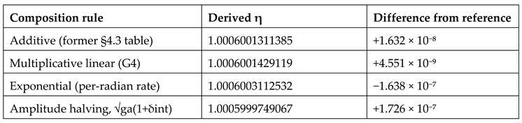
The multiplicative rule is 30 to 40 times closer than any alternative. Two independent checks concur. First, the halving theorem is proved per coefficient, which is the linear statement, and the exponential and amplitude rules contradict it at second order. Second, the transverse coefficient implied by the calibrated moves from 0.66720 under addition (0.080% above 2/3) to 0.66682 under multiplication (0.022% above 2/3); the former figure, printed as the measured coefficient in the former Section 4.3 projection table, is partly an artifact of the additive convention and is corrected in G.9.
Appendix G.5. Derived Value and the Proton
Evaluating Equation (G4) from the two inputs (CODATA 2022) and (Hanneke 2008) alone:
Through the calibration identity (H.5), the derived value predicts.

The proton mass is thus reproduced to 13.6 parts per billion with no calibration. The calibration through the proton identity remains the operational choice for the mass tables, because 13.6 ppb is roughly 230 times the CODATA uncertainty; the point of this appendix is that the calibrated quantity is now derived to within 4.6 parts per billion of itself, with the remainder characterized in G.8.
Appendix G.6. Error Budget and Audits
Three audits bound the interpretation of the remaining difference. (a) Input metrology. The derived value inherits from (dominant), , and ; the calibrated reference inherits , one third of the relative uncertainty of through the cube in the identity. The combined budget is ; the observed difference is 228 times larger and cannot be metrological. The value of entering the reference is itself a consensus over independent experimental routes (bound-electron g-factor, direct Penning-trap mass, HD+ spectroscopy) whose mutual agreement sits orders of magnitude below the required shift. (b) Reference audit. The harmonic factor 19.027314 of the proton table is exactly , reducing the calibration identity to the closed form above; independent re-inversion reproduces the quoted to . The reference carries no vintage or rounding error. Its defensible precision is . (c) Input replacement. Substituting the 2023 remeasurement of the electron anomaly for the 2008 value moves the derived by , five orders below the difference.
Appendix G.7. Alternatives Tested and Excluded
A skeptical reader will propose mechanisms for the remaining difference; those with declared physical origins were computed and are reported. Each was stated with its exact form before comparison.
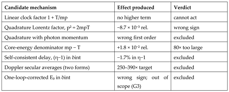
The uniform failure of kinematic dressings, together with the sign and scale pattern, constrains the true mechanism: the modulation of the sampled coupling is linear in flow energy density, not kinematic, and its correction to Equation (G3) must arise inside the secular averaging integral itself.
Appendix G.8. The Open Term: Localization and Defined Calculation
The remaining difference is stated exactly and frozen: relative to Equation (G3), the calibrated value requires an excess of , equivalently in . Its magnitude sits in the second-order regime of the internal energy fraction, , with an order-unity fractional coefficient. The calculation that decides it is defined by the Appendix E machinery: compute the secular average of the coupling sampled by the axial flow while the configuration carries the transverse ground-state motion; the first-order result must reproduce the factor of Equation (G3), and the second-order term of the same integral is then a parameter-free prediction against the frozen target. Until that integral is evaluated, the term is graded open, and no closed-form candidate is adopted. The residual does not affect any comparison in Section 8 except the proton itself: with exponents up to 9/2 across the spectrum, the worst-case consequence of the open term is 0.07 ppm, below every non-proton experimental precision in the paper.
Appendix G.9. Consequential Corrections to the Main Text (Applied in This Revision)
For internal consistency the following main-text values changed with this appendix. Former Section 4.1 and its figure caption: the external-vacuum-arrival language is replaced by the companion-flow statement of G.2; the figure geometry (contours 2π and π) is unchanged. Former Section 4.3 correction table: the composition becomes multiplicative, a cross-term row (+1.177 × 10⁻⁸) is added, the calculated value becomes 1.0006001429 and the closing accuracy 0.0045 ppm; the projection-table commentary quotes the implied coefficient 0.66682 against the derived 2/3 (0.022%). Section 7 and Appendix H.5: the calibration statement gains one sentence, that the framework-derived η reproduces the proton to 13.6 ppb before calibration, with the calibration retained for the tables. Appendix D: one clarifying sentence noting that the printed lever is algebraically equivalent to a per-flow correction on one flow of the pair taken through the exact differential of the neutron relation. No mass value, vertex function, or table entry elsewhere changes.
Appendix H. Nuances for the Discriminating Reader
This appendix addresses directly the objections that a reader trained in the Standard Model will raise first. Each is answered at its honest level, derived, argued, or open, because the framework’s credibility rests on never claiming more than it can defend.
Appendix H.1. Spin and Statistics
Two spin-1 photons do not add to spin-1/2 by angular-momentum composition, and the framework does not claim they do. The observable arises from the half-cycle coupling filter: at any instant exactly one photon of the counter-propagating pair is in the coupled half of its trajectory, and averaging over one revolution gives an externally observable angular momentum of , the same half-cycle ratio, read from a different observable, that produces the leading gyromagnetic normalization. No experiment measures the angular-momentum magnitude independently of that normalization; Stern–Gerlach establishes two projection states, not a magnitude. Independently, the parity of the selection-rule integer (Section 6.4) returns the correct statistics for every particle tested, including the neutral pion.
Appendix H.2. Lepton and Baryon Number
Neither is a primitive here. They are bookkeeping labels for closure topology: planar closed orbits (charged leptons), tri-flow spherical closures (baryons), open helices (neutrinos). Their conservation is topological protection at the level argued in H.3, a structural obstruction, not yet a theorem, and the framework states this plainly rather than importing the conservation laws as unexplained axioms.
Appendix H.3. Proton Stability
The sharpest available objection: if the proton is an orbital configuration of the same object as the electron, what forbids ? The decay releases 803 MeV, both products exist in this spectrum, and experiment demands protection at yr (Super-Kamiokande). Nothing energetic protects the proton; the protection is structural. For the boundary condition requires all three orthogonal projections simultaneously occupied (Section 6.4); a partially dismantled configuration, two flows under a spherical boundary, is not a closure solution, so no intermediate state exists. The neutron comparison isolates the point: neutron beta decay sheds an attachment while the core persists intact through the decay; has no such channel, because its final state, a planar closed orbit plus a single kernel, contains no tri-flow object, so the decay requires unwinding the simultaneous three-flow lock in one step, through configurations the closure condition excludes. Stated honestly: this is a qualitative topological obstruction, not a computed lifetime. The amplitude for a single-step reorganization, and the lifetime bound it implies, are open item O-B. The per-particle selection integer supplies no additive vertex conservation law and is not claimed as the protection.
Appendix H.4. The Relation to QCD
This paper computes mass values; it does not address confinement, asymptotic freedom, or parton distribution functions, and does not claim to replace QCD dynamics (Section 1.2). The claim is narrower: the observed mass hierarchy admits a parallel geometric account at the stated precision. Whether QCD and this description are alternative accounts of one underlying dynamics is a genuine open question, flagged in the Conclusion, and nothing in this paper depends on its answer.
Appendix H.5. The Eleven-Figure Suspicion
A precision claim far beyond lattice QCD rightly invites the search for tuning, and the paper anticipates the search by disclosing its own structure. The proton agreement is a fixed point of the – relation, in which depends on through the residual; the genuinely independent tests are therefore the neutron (with computed independently of ), the pion, and the top quark. Every closing coefficient is independently sourced: from QED, and and the transverse weight 2/3 derived from the flow assignment of the leading term. For the reader unwilling to adopt the model at all, three relations are checkable in an afternoon from tabulated constants alone, , with , and , together with the calibration identity , which exhibits exactly how is fixed by the proton, and they stand or fall independently of the picture that produced them.
Appendix H.6. What Would Falsify This
The tauon second-harmonic prediction, 3477.2269 , resolvable by Belle II (Section 8.1); the pion prediction MeV under improved pionic-atom spectroscopy; observation of proton decay at rates implying an unobstructed reorganization; and the two named calculations the framework owes, the frozen-polarization energy of the neutral pion (O-) and the proton-reorganization amplitude (O-B). A framework that reaches this far must state where it can be killed; these are the places.
Appendix H.7. Why There Is No Energy-Field Lagrangian, and What Replaces It
A recurring demand deserves a direct answer rather than deferral. A Lagrangian density presupposes a continuous energy field defined at every point of spacetime, smooth enough to vary; the Euler–Lagrange equations are a theorem about such fields. This framework’s ontology contains no such object: energy resides in the photons themselves, the vacuum carries probability-flow density rather than energy density, and binding operates through the local change in propagation speed rather than through potential energy. There is no kinetic-minus-potential density to write and no field configuration to vary. The demand for an energy-field Lagrangian is therefore a category error with respect to this ontology, not an incompleteness the framework concedes.
What replaces the missing object, phase stationarity as the native variational law, the reassignment of gauge freedom to the physical duality angle of the photon pair, the non-Lagrangian residence of the conservation laws and the virial theorem, and the global-closure lawform itself, is developed in the companion Delta-c record [1,2,17], building on the Wheeler and Feynman precedent of field-free electrodynamics [21]. None of that argument is needed here: the mass-spectrum proposition of this paper is tested by Section 2 through 8 and stands or falls on that arithmetic alone.
References
- Froedge, D.T. Vacuum Polarization, Gravitation, Charge and the Speed of Light. 2021. Available online: http://www.arxdtf.org/outLibrary/book_one (accessed on 11 August 2026).
- Froedge, D.T. Physics Without Energy Fields or Charge. 2022. Available online: http://www.arxdtf.org/outLibrary/book_two (accessed on 11 August 2026).
- Barut, A.O. Lepton Mass Formula. Phys. Rev. Lett. 1979, 42, 1251. [Google Scholar] [CrossRef]
- Barut, A.O. Stable Particles as Building Blocks of Matter. Surv. High Energy Phys. 1980, 1, 113. [Google Scholar] [CrossRef]
- Hestenes, D. The Zitterbewegung Interpretation of Quantum Mechanics. Found. Phys. 1990, 20, 1213. [Google Scholar] [CrossRef]
- Williamson, J.G.; van der Mark, M.B. Is the Electron a Photon with Toroidal Topology? Ann. Fond. Louis Broglie 1997, 22, 133. [Google Scholar]
- Harari, H. A Schematic Model of Quarks and Leptons. Phys. Lett. B 1979, 86, 83. [Google Scholar] [CrossRef]
- Shupe, M.A. A Composite Model of Leptons and Quarks. Phys. Lett. B 1979, 86, 87. [Google Scholar] [CrossRef]
- Hooft, G. Naturalness, Chiral Symmetry, and Spontaneous Chiral Symmetry Breaking. In Recent Developments in Gauge Theories; Plenum Press: New York, NY, USA, 1980. [Google Scholar]
- Aoyama, T.; Kinoshita, T.; Nio, M. Theory of the Anomalous Magnetic Moment of the Electron. Atoms 2019, 7, 28. [Google Scholar] [CrossRef]
- Froedge, D.T. Exact All-Orders Reconciliation of Atomic and Nuclear Kernels in Delta-c Mechanics. 2026. Available online: http://www.arxdtf.org (accessed on 11 August 2026).
- Källén, G.; Sabry, A. Fourth Order Vacuum Polarization. Dan. Mat. Fys. Medd. 1955, 29, 17. [Google Scholar]
- Schwinger, J. On Quantum-Electrodynamics and the Magnetic Moment of the Electron. Phys. Rev. 1948, 73, 416. [Google Scholar] [CrossRef]
- Mohr, P.J.; Newell, D.B.; Taylor, B.N.; Tiesinga, E. CODATA Recommended Values of the Fundamental Physical Constants: 2022. Rev. Mod. Phys. 2025, 97, 025002. [Google Scholar] [CrossRef]
- Eidelman, S.; Passera, M. Theory of the τ Lepton Anomalous Magnetic Moment. Mod. Phys. Lett. A 2007, 22, 159. [Google Scholar] [CrossRef]
- Particle Data Group; Navas, S.; et al. Review of Particle Physics. Phys. Rev. D. 2024, 110, 030001. [Google Scholar] [CrossRef]
- Froedge, D.T. The Neutrino as a Two-Photon Open Helical Orbit: Mass Scale, Tetrahedral Mixing, and Majorana Character. 2026. Available online: http://www.arxdtf.org (accessed on 11 August 2026).
- Froedge, D.T. Hydrogen Fine Structure by an Alternate Interpretation of the Feynman Path Integral. Phys. Essays 2026. accepted for publication. [Google Scholar]
- Aker, M.; et al. (KATRIN Collaboration) Direct Neutrino-Mass Measurement with Sub-Electronvolt Sensitivity. Nat. Phys. 2022, 18, 160. [Google Scholar] [CrossRef]
- Eddington, A.S. Fundamental Theory; Cambridge University Press: Cambridge, UK, 1946. [Google Scholar]
- Wheeler, J.A.; Feynman, R.P. Interaction with the Absorber as the Mechanism of Radiation. Rev. Mod. Phys. 1945, 17, 157. https://doi.org/10.1103/RevModPhys.17.157. Wheeler, J.A.; Feynman, R.P. Classical Electrodynamics in Terms of Direct Interparticle Action. Rev. Mod. Phys. 1949, 21, 425. https://doi.org/10.1103/RevModPhys.21.425.
Disclaimer/Publisher’s Note: The statements, opinions and data contained in all publications are solely those of the individual author(s) and contributor(s) and not of MDPI and/or the editor(s). MDPI and/or the editor(s) disclaim responsibility for any injury to people or property resulting from any ideas, methods, instructions or products referred to in the content. |
© 2026 by the authors. Licensee MDPI, Basel, Switzerland. This article is an open access article distributed under the terms and conditions of the Creative Commons Attribution (CC BY) license (http://creativecommons.org/licenses/by/4.0/).
Copyright: This open access article is published under a Creative Commons CC BY 4.0 license, which permit the free download, distribution, and reuse, provided that the author and preprint are cited in any reuse.