

Submitted:
11 August 2026
Posted:
12 August 2026
You are already at the latest version
Abstract
Clonogenic survival under fractionated irradiation flattens after one to two weeks at a level that depends on fraction size. The linear–quadratic (LQ) model cannot reproduce this, because its exponent is a linear functional of delivered dose and therefore carries no memory of how the dose was given. We construct the smallest kill law that can, from six axioms: two clonogenic states, first-order kill in each, a constant ratio between their kill rates, a causal damage-driven transfer between them, conservation of total transfer, and one-way transfer over the interval considered. We prove the axioms independent, and prove that they determine the structural results without specifying either the hazard or the transfer kernel. These give a five-variable initial-value problem — a lethal hazard carrying a Lea–Catcheside repair memory, a two-stage cascade converting accumulated damage into transfer, and the two clonogenic compartments — which we solve in closed form for arbitrary dose rate. Two exact properties carry the results. The transfer term cancels identically when the two compartments are equally radiosensitive, so survival then depends only on the repair-weighted cumulative lethality; delivery order therefore changes cell kill if and only if a tolerance gap exists, provided repair is complete between deliveries. And once transfer is complete the per-fraction log-kill falls from L to rL, so late dose is devalued by r, tumour volume is amplified by 1/r, and cytoreduction is worth 1/r times its conventional value. For instantaneous fractions separated by intervals long compared with the repair and signal time constants, the system reduces exactly to a two-by-two linear map, verified to machine precision. Fitted to clonogenic survival at five fraction sizes the model returns a gate time constant of 1.75 fractions and a tolerance ratio of 0.063, with a held-out quantity implying 1.84 and excluding zero delay; we also report that it generalises slightly worse than a hand-added floor when whole fraction sizes are withheld. Away from that limit the formulation yields results a fraction-based law cannot express. Continuous low-dose-rate irradiation is penalised twice, by repair and by allowing the transfer time to act during delivery, and a seven-day implant delivering 60 Gy is predicted to be equivalent to thirty 2 Gy fractions. For radionuclide therapy, cell kill is predicted to rise by more than four log-kill as the effective half-life falls from thirty days to six hours at matched absorbed dose, so absorbed dose alone is an insufficient basis for comparing agents. The heterogeneity of uptake in radionuclide therapy also supplies the one configuration in which the tolerance ratio becomes measurable in vivo, because the dose-rate contrast between regions is known from the dosimetric imaging itself. The construction is calibrated on one cell line and the tolerance ratio has never been measured on a clonogenic endpoint; the claims that survive this are structural.
Keywords:
fractionation
; cell survival
; radiation tolerance
; dose rate
; brachytherapy
; radionuclide therapy
1. Introduction
1.1. A Model Built on a Frozen Cell
The quantitative description of radiation cell killing began with target theory, in which survival is set by the statistics of energy deposition in a small number of sensitive volumes (Lea and Catcheside 1942). Two developments in the early 1970s converted that idea into the form still used clinically. Kellerer and Rossi (1972) derived, from microdosimetric considerations, that lesion yield should be proportional to αD + βD2, with the quadratic term arising from the pairwise combination of sublesions produced by separate energy-deposition events. Chadwick and Leenhouts (1973) reached the same expression from a molecular argument in which the two terms correspond to double-strand breaks produced by one track and by two tracks respectively. The resulting linear–quadratic (LQ) expression gives the surviving fraction after a single acute dose d as S = exp[−(αd + βd2)], and for n identical well-separated fractions
−ln S(n) = n(αd + βd2) ≡ nL .(1)
Equation 1 has organised clinical fractionation for five decades (Fowler 1989; Brenner 2008; McMahon 2019). Its success rests on being embedded in a wider account of what happens between fractions rather than during them: the four Rs of repair, redistribution, repopulation and reoxygenation (Withers 1975), each of which modifies α, β or the effective number of clonogens without altering the functional form. Sublethal repair was incorporated by making the quadratic term depend on the temporal pattern of delivery through the Lea–Catcheside factor (Dale 1985, 1986), and accelerated repopulation by adding a time-dependent term (Withers et al. 1988). The framework has proved remarkably durable under extension.
What has not been extended is the assumption underneath it. In Eq. 1 the radiosensitivity coefficients are constants of the cell, fixed before treatment and unaltered by it. The exponent is therefore a linear functional of the delivered dose, and three properties follow from that structure alone rather than from any measurement: log-kill is linear in fraction number, biologically effective dose is additive across a course, and survival is unchanged if the fractions are reordered. The first two are used constantly in practice; the third is rarely tested, because delivery order is rarely varied.
1.2. Where the Frozen-Cell Assumption Has Been Questioned
Departures from Eq. 1 have been recognised for as long as it has been used, and the responses have been informative about what the field is willing to change. At large doses per fraction the predicted curve continues to bend where measured survival becomes more nearly log-linear, and this has been addressed either by declaring the model inapplicable above some dose (Kirkpatrick et al. 2008) or by defending it and attributing the discrepancy to other causes (Brenner 2008). The clinical time factor was addressed by adding a repopulation term rather than by revisiting the kill law (Withers et al. 1988). In each case the response has been to modify the parameters or append a term, leaving the underlying assumption that the cell’s radiosensitivity is a fixed property untouched.
That assumption is difficult to sustain against a specific observation. Van den Berg et al. (2020) followed clonogenic survival through thirty fractions in seven cell lines under clinically patterned delivery and found that the curves do not continue to fall. They flatten after one to two weeks; the level at which they flatten depends on the size of the fraction; and the effect reverses only after a recovery period. Every line ends far above its own extrapolation from Eq. 1, by factors between 103 and 105. No adjustment of α and β reproduces this, because a plateau requires the exponent to stop growing with dose, and in Eq. 1 it cannot: the exponent is linear in delivered dose by construction.
1.3. Induction or Selection
Two mechanisms could produce such a plateau, and the distinction matters clinically because only one is in principle preventable. Under selection, a resistant subpopulation is present before treatment and is progressively enriched by differential killing; the survival curve then flattens as the population composition shifts, and the tolerance is a property the tumour brought with it. Under induction, irradiation writes a tolerant state that did not previously exist. The fractionation data alone do not separate them, since both accounts can be fitted.
Direct evidence has accumulated for induction, and it is worth distinguishing its strands. In the radioadaptive response, a priming dose too small to kill an appreciable fraction of the population confers protection against a later challenge, and the protection appears only when the challenge is delayed (Olivieri et al. 1984); because a priming dose of that size leaves essentially nothing for differential killing to enrich, the observation is difficult to attribute to selection. In cancer cells exposed to cytotoxic drugs, a reversible tolerant state adopted by a subpopulation was characterised as chromatin-mediated (Sharma et al. 2010) and later shown to carry targetable vulnerabilities (Hangauer et al. 2017; Russo et al. 2024). For irradiation specifically, tolerant populations have now been isolated as physical entities rather than inferred from curve shape: Gu et al. (2022) generated one from a glioblastoma xenograft by successive irradiation and characterised it transcriptionally and functionally, Zhao et al. (2023) isolated a corresponding population in colorectal carcinoma and demonstrated its reversion, and Forissier et al. (2025) established by lineage tracing that such cells arise from the treated population rather than from a distinct pre-existing lineage.
1.4. What a Kill Law Must Carry, and over What Range
Accepting induction requires a kill law that carries state: the population must be described by more than a single number, and the effect of a dose increment must depend on what the preceding dose has already done. The minimal such law acts between instantaneous fractions and is a two-by-two linear map. That is sufficient for conventional external-beam fractionation, and it is not sufficient in general, for a reason that is structural rather than practical. A transfer driven by accumulated damage carries no clock, so survival depends only on total lethality and is identical at every dose rate. A formulation of that kind cannot represent sublethal repair without pre-computing it externally, and cannot represent continuous irradiation at all — neither brachytherapy, where dose is delivered over hours to days (Dale 1985), nor radionuclide therapy, where the dose rate decays with an effective half-life and absorbed dose is the standard basis for prescribing (Sgouros et al. 2020). These are not marginal cases: they are a growing share of practice, and they are precisely the regimes in which the interaction between delivery time and an induced state would be largest.
We therefore work in continuous time throughout. Section 2 states six axioms, establishes their independence and proves a completeness theorem, and derives the system they imply; Section 3 solves it in closed form for arbitrary dose rate; Section 4 shows that a two-by-two map between fractions is an exact limit; Section 5 proves the two properties that carry the results. Section 6 calibrates against fractionated survival data and reports two held-out tests and one clear negative. Section 7 to 12 work out the consequences for conventional fractionation, delivery time, brachytherapy, radionuclide therapy, radiation quality, and for measuring the governing parameter in a patient. Section 13 to 15 give the falsifiable predictions, the limitations, and the single experiment that would confirm or refute the mechanism.
2. Derivation of the Continuous-Time System
2.1. Axioms
We state the postulates as axioms in the sense used for applied formal systems: primitive propositions, assumed rather than derived, from which the results of Section 3 and Section 5 follow by deduction, and for which independence and completeness can be checked. They are empirical claims about biology, not logical necessities. Section 2.2 gives the evidence for each, Section 2.3 establishes their independence, and Section 2.4 states what they do and do not determine.
Let Ns(t) and Np(t) denote the two clonogenic sub-populations and let h(t) ≥ 0 denote the instantaneous lethal hazard, an integrable function of time determined by the delivery.
Axiom 1 (two-state resolution). The clonogenic population is exhaustively partitioned into two states at every instant, so that T = Ns + Np.
Axiom 2 (first-order kill). Each state is depleted by irradiation at a rate proportional to its own population, with the same hazard function h up to a constant of proportionality.
Axiom 3 (proportional tolerance). The constant of proportionality for the tolerant state is r, independent of time, dose and dose rate, with 0 ≤ r ≤ 1.
Axiom 4 (causal damage-driven transfer). The transfer rate w(t) from the sensitive to the tolerant state is a causal, linear, time-invariant functional of the hazard: w(t) = ∫0ᵗ K(t−s) h(s) ds for some non-negative kernel K supported on t ≥ 0.
Axiom 5 (transfer conservation). The kernel is normalised, ∫0∞ K(u) du = κ, so that a given quantity of lethality eventually transfers a fixed proportion of the surviving sensitive population.
Axiom 6 (one-way transfer). No transfer occurs from the tolerant to the sensitive state over the interval considered.
These six axioms give
dNs/dt = −[h(t) + w(t)] Ns , dNp/dt = −r h(t) Np + w(t) Ns ,(2)
which is Eqs. 6 and 7 of Section 2.7 with ρ = 0. Nothing in Axioms 1–6 specifies either the hazard h or the kernel K; both are supplied separately in Section 2.5 and Section 2.6, and Section 2.4 shows why that separation matters.
2.2. Justification of the Axioms
Axiom 1. The two-state resolution is unusual among modelling postulates in radiobiology in that the states have been isolated as physical populations rather than inferred from the shape of a survival curve. Gu et al. (2022) generated a tolerant population from a glioblastoma xenograft by successive rounds of irradiation and characterised it transcriptionally and functionally, showing that it differs from the parental population in colony-forming behaviour as well as in phenotype, and that it persists across seven-day gaps between rounds and through re-implantation. Zhao et al. (2023) isolated a corresponding population in colorectal carcinoma and demonstrated that it reverts, which establishes it as a state rather than a lineage. Forissier et al. (2025) tracked its emergence by lineage tracing, which is the observation that most directly excludes the alternative that the tolerant cells were a distinct pre-existing subclone: they arise from the treated population. The same behaviour is long established for cytotoxic drug exposure, where the tolerant condition was first described as chromatin-mediated and reversible (Sharma et al. 2010) and subsequently shown to carry targetable vulnerabilities (Hangauer et al. 2017; Russo et al. 2024). What Axiom 1 adds beyond these observations is only that two states suffice; a third would not be excluded by the data, and we adopt two as the minimal choice that can produce the phenomenon of Section 1.2.
Axiom 2. First-order kill is the standard kinetic assumption of the field and is inherited rather than introduced here. It underlies target theory (Lea and Catcheside 1942) and both derivations of the linear–quadratic form, the microdosimetric (Kellerer and Rossi 1972) and the molecular (Chadwick and Leenhouts 1973), in each of which the surviving fraction is exponential in a lesion yield. Axiom 2 asserts only that this holds separately within each of the two states of Axiom 1, with a common hazard function up to a constant. It carries no commitment to the functional form of that hazard, which is why Theorem 1 does not depend on the linear–quadratic expression.
Axiom 3. This is the least secure of the six and should be read as the principal structural commitment rather than a normalisation. It asserts that the tolerant state is harder to kill by a constant factor, so that the ratio of the two kill rates does not change with dose, dose rate or time. Expressed in linear–quadratic terms it is equivalent to tolerance acting multiplicatively on both radiosensitivity coefficients, rα = rβ, which has not been measured. The direct evidence is indirect: colony formation differs between successive tolerant populations at matched seeding density (Gu et al. 2022), which establishes a difference in clonogenic behaviour but does not establish that the difference is a constant multiple. Two considerations motivate it nonetheless. It is the weakest assumption under which the two-mode structure of Section 5.2 exists at all, since any state-dependent kill law with a fixed ratio yields two decay modes. And it is testable directly, by measuring the survival curves of sorted tolerant and parental populations at several doses and asking whether the ratio of their log-kills is constant. Section 2.3 shows that Theorem 1 fails if it is relaxed, which is what makes it worth testing rather than assuming.
Axioms 4 and 5. Together these say that the transfer is driven by delivered damage, follows it in time, and conserves a fixed proportion per unit lethality. The causal and damage-driven character is supported by the observation that a tolerant population appears after irradiation and after a small number of fractions rather than being present beforehand: three fractions of 2 Gy suffice in the system of Gu et al. (2022), and the phenotype of Van den Berg et al. (2020) develops over one to two weeks of fractionated delivery. The linearity and time-invariance of the functional are the minimal choices consistent with that observation, and are what make the transfer expressible as a convolution. Axiom 5 is a normalisation: without it the kernel could be scaled arbitrarily and the transfer per fraction would not converge, so the discrete limit of Section 4 would not exist. Neither axiom specifies the kernel, and Section 2.4 shows that no result of Section 5 depends on it.
Axiom 6. Reversion is not absent, and Axiom 6 is an approximation whose validity condition is explicit: it requires the interval between deliveries to be short compared with the reversion half-life. That condition is supported for conventional fractionation. Van den Berg et al. (2020) find that the acquired resistance reverses only after a recovery period, having persisted through thirty fractions of continued irradiation; Zhao et al. (2023) report reversion over days to weeks; Gu et al. (2022) maintain the phenotype across seven-day gaps and through re-implantation. For daily delivery the condition therefore holds comfortably. It fails for pulsed schedules with intervals of weeks, and Section 7.4 restores the reversion term for that case rather than treating the axiom as universal. We retain ρ explicitly in Eqs. 6 and 7 so that the approximation can be tested rather than assumed.
One general remark applies to all six. The evidence for Axioms 1, 4 and 6 is direct and specific to irradiated tumour cells; the evidence for Axiom 2 is inherited from the standard model; Axiom 5 is a normalisation; and Axiom 3 is the one that rests on the least direct support while carrying the most structural weight. That asymmetry is deliberate and is the reason the discriminating experiment of Section 13 targets the consequence of Axiom 3 rather than the existence of the two states, which is no longer in serious doubt.
2.3. Independence
An axiom set is independent if no member follows from the others. Independence is established here by exhibiting, for each axiom, a system satisfying the remaining five in which a result of Section 5 fails.
Dropping Axiom 1 leaves a single compartment, for which the survival exponent is ∫h dt and no plateau is possible at any parameter values, so the phenomenon of Section 1.2 becomes inexpressible. Dropping Axiom 2 removes the linearity on which the integrating factor of Section 3.1 depends and no closed form exists. Axiom 3 is independent of Axiom 2, which is easily overlooked because both concern the kill rates: Axiom 2 asserts first-order kinetics within each state, Axiom 3 asserts that the ratio between the two rates is a constant. Allowing r to depend on dose while retaining all other axioms breaks the invariant. We verified this numerically: over all 120 permutations of a five-fraction sequence the ratio of maximum to minimum survival is 1.000000000000 with r constant and 1.0059 with r varying linearly with fraction size.
Dropping Axiom 4 permits a transfer rate depending on quantities other than the delivered hazard — elapsed time, or the tolerant population itself — in which case the transfer terms of Eq. 2 no longer cancel on addition and Theorem 1 fails. Dropping Axiom 5 leaves κ undefined and the discrete limit of Section 4 does not exist, since the between-fraction transfer no longer converges to a fixed proportion. Dropping Axiom 6 introduces a reversion term; the closed form of Section 3.1 is lost, although Theorem 1 survives, so this axiom is independent of the others but is required for the solution rather than for the structural results.
2.4. Completeness
Axioms 1–6 determine the system only up to two objects: the hazard h, which is a property of the radiation and the cell rather than of the tolerance mechanism, and the kernel K, of which the cascade of Section 2.6 is one admissible choice among infinitely many. The axiom set is therefore not complete in the sense of specifying a unique model. It is complete in a weaker and more useful sense, which we state as a theorem.
Theorem 1 (invariance and sufficiency). Under Axioms 1–6, for any integrable hazard h ≥ 0 and any admissible kernel K: (i) the total population obeys dT/dt = −h(t)[Ns + rNp], in which K does not appear; (ii) if r = 1 then T(t) = T(0)exp[−∫0ᵗ h], so survival depends on the delivery only through the cumulative hazard and is invariant under any rearrangement of the delivery that preserves it; and (iii) under repeated identical delivery the log-kill per delivery converges to r times its sensitive value. None of (i)–(iii) depends on the form of h or of K.
Proof. (i) Adding the two equations of Eq. 2 gives dT/dt = −hNs − wNs − rhNp + wNs; the transfer terms cancel identically, leaving dT/dt = −h(Ns + rNp). Since w does not appear, neither does K. (ii) Setting r = 1 in (i) gives dT/dt = −hT, which integrates to the stated form, whose right-hand side depends on the delivery only through ∫h. (iii) The system of Eq. 2 has decay modes e−∫h and e−r∫h; for r < 1 the second is the slower and dominates as the cumulative hazard grows. ∎
Three consequences follow. First, the axiom set is complete for the structural results: no further postulate is required to obtain the ablation null or the asymptotic law, and neither depends on radiation being described by a linear–quadratic hazard. We verified this by evaluating the null under linear, linear–quadratic, cubic and saturating hazards, obtaining a permutation ratio of 1.000000000000 in every case, with the asymptotic log-kill agreeing with r times the sensitive value to six decimal places throughout. Second, the hazard and the kernel are required only for quantitative predictions, so a reader who rejects the linear–quadratic form or the particular cascade may still accept the structural results. Third, the magnitudes do depend on the kernel: the same order contrast returns 0.945 under a single-exponential kernel, 0.980 under the two-stage cascade and 0.953 under a rectangular kernel, so quantitative claims carry a modelling commitment that the structural claims do not.

Table 1.
Structural summary of the axiom set. Section 2.2 gives the evidence in full, Section 2.3 the independence argument, and Section 2.4 the completeness theorem. The final row records the two objects the axioms deliberately leave unspecified.
Table 1.
Structural summary of the axiom set. Section 2.2 gives the evidence in full, Section 2.3 the independence argument, and Section 2.4 the completeness theorem. The final row records the two objects the axioms deliberately leave unspecified.
| Axiom | Statement | Status of evidence | Principal sources | Failure mode |
|---|---|---|---|---|
| 1 | Two clonogenic states | Direct; populations isolated | Gu 2022; Zhao 2023; Forissier 2025; Sharma 2010 | No plateau possible |
| 2 | First-order kill in each state | Inherited from standard model | Lea and Catcheside 1942; Kellerer and Rossi 1972; Chadwick and Leenhouts 1973 | No closed-form solution |
| 3 | Kill-rate ratio r is constant | Weakest; equivalent to rα = rβ, untested | Gu 2022 (partial) | Theorem 1(ii) fails; permutation ratio 1.0059 |
| 4 | Transfer is a causal linear functional of the hazard | Direct; transfer follows dose | Gu 2022; Van den Berg 2020 | Transfer terms do not cancel; Theorem 1(i) fails |
| 5 | Total transfer per unit lethality is κ | Normalisation | — | Discrete limit does not exist |
| 6 | Transfer is one-way over the interval | Direct, with stated validity condition | Van den Berg 2020; Zhao 2023; Gu 2022 | Closed form lost; Theorem 1 survives |
| — | Hazard h and kernel K (supplied separately) | Modelling choices | Lea and Catcheside 1942; Dale 1985, 1986; Olivieri 1984 | Nothing structural; magnitudes only |
2.5. The Lethal Hazard
Let Ḋ(t) be the dose rate and D(t) the dose delivered by time t. Under the standard treatment of sublethal damage interaction, the instantaneous rate of lethal lesion production is
h(t) = αḊ(t) + 2βḊ(t) q(t) , dq/dt = Ḋ(t) − μq(t) , q(0) = 0 ,(2)
where q(t) is the concentration of unrepaired sublethal damage and μ = ln2/t½ʳᵉᵖ is the repair rate. Integrating Eq. 2 for an acute dose delivered in a time short compared with 1/μ gives q → D and ∫h dt → αD + βD2, recovering the acute LQ exponent; for a protracted delivery it gives the Lea–Catcheside form. We write H(t) = ∫0ᵗ h(t′)dt′ for the cumulative lethality.
2.6. The Signalling Cascade
Let σ(t) be a fast damage signal and γ(t) a slower gate variable:
dσ/dt = h(t) − σ/τσ , dγ/dt = σ/τσ − γ/τγ , σ(0) = γ(0) = 0 ,(3)
with τσ ≪ τγ. The transfer rate from the sensitive to the tolerant compartment is taken proportional to the gate,
w(t) = κ γ(t)/τγ .(4)
The cascade of Eqs. 3–4 conserves total transfer. Integrating the first of Eq. 3 over all time gives ∫(σ/τσ)dt = ∫h dt, since σ returns to zero; integrating the second gives ∫(γ/τγ)dt = ∫(σ/τσ)dt. Hence
∫0∞ w(t) dt = κ ∫0∞ h(t) dt = κ H(∞) ,(5)
independently of τσ and τγ. The time constants therefore set when the transfer occurs but not how much occurs in total, which is what makes the reduction of Section 4 exact.
The two-stage cascade of Eq. 3 is the minimal structure that produces a delay while satisfying Axioms 4 and 5. It arises as a reduction of a wider layered description of radiation response, in which processes are ordered by relaxation time from redox chemistry through damage signalling to clonal dynamics, and in which successive quasi-steady-state elimination of the faster layers leaves the two-compartment core used here (Vaitheeswaran 2026a). That description is not required for any result in this paper: by Theorem 1 the structural results hold for any admissible kernel, and the cascade is one such choice. We refer to it only to record where the two time constants come from and what they correspond to physically.
2.7. The Full System
Combining Axioms 1–6 and Eqs. 2–4, the state (Ns, Np, σ, γ, q) evolves as
dNs/dt = −[h(t) + w(t)] Ns + ρ Np ,(6)
dNp/dt = −r h(t) Np + w(t) Ns − ρ Np ,(7)
together with Eqs. 2 and 3, where ρ is the reversion rate, set to zero under Axiom 6 and retained so that the assumption can be tested. Equations 2, 3, 6 and 7 constitute the model. The surviving fraction is SF(t) = [Ns(t) + Np(t)]/[Ns(0) + Np(0)], evaluated after the cascade has relaxed so that the transfer implied by Eq. 5 is complete.
3. Solution
3.1. Closed Form for Arbitrary Delivery
Equations 6 and 7 with ρ = 0 form a lower-triangular linear system, so they integrate exactly for any Ḋ(t). Define
Φ(t) = ∫0ᵗ [h(t′) + w(t′)] dt′ , Ψ(t) = r ∫0ᵗ h(t′) dt′ = r H(t) .(8)
With the definitions of Eq. 8, Eq. 6 is separable and gives
Ns(t) = Ns(0) e−Φ(t) .(9)
Substituting Eq. 9 into Eq. 7 and multiplying by the integrating factor eΨ(t),
d/dt [ eΨ(t) Np(t) ] = eΨ(t) w(t) Ns(0) e−Φ(t) ,(10)
Integrating Eq. 10 from 0 to t gives
Np(t) = e−Ψ(t) { Np(0) + Ns(0) ∫0ᵗ w(u) eΨ(u) − Φ(u) du } .(11)
Equations 9 and 11 are the general solution. They require no assumption about the delivery pattern: Ḋ(t) may be a train of fractions, a constant low dose rate, or an exponentially decaying source, and h, w, Φ and Ψ follow from Eqs. 2–4.
3.2. The Frozen-Cascade Limit
When the cascade is fast compared with the delivery (τσ, τγ → 0), Eq. 4 gives w → κh, so Φ → (1+κ)H and Ψ → rH. The integral in Eq. 11 then has the closed form
∫0ᵗ κh e(r−1−κ)H du = κ [ e(r−1−κ)H(t) − 1 ]/(r−1−κ) ,(12)
using dH = h du. Since r < 1 and κ > 0 the denominator is strictly negative and the expression is regular. Substituting Eq. 12 into Eq. 11,
SF(t) = e−(1+κ)H + κ [ e−rH − e−(1+κ)H ]/(1+κ−r) ,(13)
for an initially sensitive population, where H = H(t). Equation 13 is the continuous analogue of the discrete closed form and depends on the delivery only through H. Setting r = 1 in Eq. 13 collapses the two exponentials and returns e−H, which is Eq. 18.
4. Exact Reduction to the Discrete Map
Consider a course of fractions of doses d1 … dN delivered at intervals Δt satisfying Δt ≫ 1/μ (repair complete) and Δt ≫ τσ (fast signal relaxed), with each delivery short compared with all time constants. Within a delivery, w is negligible because γ has not yet responded, so Eqs. 6 and 7 give
Ns → Ns e−Lk , Np → Np e−rLk , Lk = αdk + βdk2 ,(14)
and σ jumps by Lk by Eq. 3. Between deliveries h = 0, so Eqs. 6 and 7 reduce to dNs/dt = −wNs and dNp/dt = +wNs: the transfer continues after the beam is off, with no further killing. Writing Wk = ∫ w dt over the interval, the between-fraction step is
Ns → e−Wk Ns , Np → Np + (1 − e−Wk) Ns .(15)
By Eq. 5, Wk → κLk once the cascade has relaxed. Composing Eqs. 14 and 15 and writing Ak = e−Lk, Bk = e−rLk and Ck = e−κLk gives
Ns(k+1) = Ak Ck Ns(k) , Np(k+1) = Bk Np(k) + Ak(1−Ck) Ns(k) ,(16)
which is a two-by-two linear map acting between fractions. The reduction is exact rather than approximate, and the consolidation window familiar from fraction-based descriptions is not an independent parameter here but the number of fractions over which γ accumulates, set by τγ. We verified Eq. 16 against numerical integration of Eqs. 2–3 and 6–7 for eight dose sequences spanning 1 to 4 Gy per fraction and 1 to 30 fractions; the largest relative discrepancy was 6 × 10⁻¹⁶, at the level of floating-point round-off.
Two consequences of the derivation are worth stating, because a fraction-based description cannot express either. First, the transfer completes after the beam is off (Eq. 15), so the tolerance written by a fraction is realised during the following interval rather than during delivery. Second, Eq. 16 holds only in the limit of complete inter-fraction repair; when Δt is not large compared with 1/μ, Eq. 2 carries damage forward and Eq. 14 fails (Dale 1986).
5. Structural Results
5.1. The Ablation Null
Let T = Ns + Np. Adding Eqs. 6 and 7 with ρ = 0, the transfer terms ∓w Ns cancel identically and
dT/dt = −h(t) Ns − r h(t) Np .(17)
The coefficient κ does not appear in Eq. 17, so the total population is insensitive to the transfer rate and depends on the schedule only through the difference between the two kill rates. If r = 1, Eq. 17 becomes dT/dt = −h(t)T, which integrates to
T(t) = T(0) exp[−H(t)] .(18)
Equation 18 states that at the ablation locus the population follows the linear–quadratic law of Eq. 1 exactly, with H in place of nL.
Corollary 1. With the linear–quadratic hazard of Eq. 2, total clonogenic survival depends on the delivery only through the repair-weighted cumulative lethality H if and only if r = 1. This is Theorem 1(ii) specialised to that hazard; the converse follows because for r < 1 the two terms of Eq. 17 carry different coefficients, so the partition of T between the compartments when a dose increment is delivered alters its contribution, and that partition depends on the preceding history.
The corollary that survival is invariant under permutation of the fractions requires one further condition, which is easily overlooked. Permuting fractions leaves H unchanged only when repair is complete between them, since otherwise q in Eq. 2 carries damage across the interval and H itself becomes order-dependent. We verified both statements numerically: over all 120 permutations of a five-fraction sequence with 24-hour intervals, the ratio of maximum to minimum survival was 1.0000000000000004 at r = 1 and 1.171 at r = 0.063; with one-hour intervals and a 30-minute repair half-time the ratio at r = 1 was 1.375, the residual order dependence being entirely attributable to incomplete repair. The keystone experiment of Section 10 must therefore use inter-fraction intervals long compared with the repair half-time, or the null will not be observed even when the mechanism is absent.
5.2. The Asymptotic Law
For a repeated identical delivery, Eq. 17 has two modes, e−H and e−rH. Since r < 1 the second decays more slowly and dominates asymptotically, so the log-kill per fraction falls from L to rL. Three clinical consequences follow from this limit alone, since they depend only on the ratio of the two modes. Dose delivered after the transfer is complete is devalued by r. The dose achieving fifty per cent control rises with the logarithm of tumour volume at 1/r times the linear–quadratic rate, so doubling volume costs 2.3 Gy under Eq. 1 and between 4.7 and 37 Gy here. And a reduction of clonogen burden by a factor ψ contributes ln ψ to the control exponent directly, without passing through the kill law, so the dose achieving the same effect is (1/r) times its conventional value: cytoreduction acts on the initial clonogen number and is undevalued, whereas dose acts through L and is devalued by r.
6. Calibration and Tests Against Data
The parameters were obtained by fitting to clonogenic survival of the U-251MG glioblastoma line under fractionated irradiation at five fraction sizes (1.8, 2.0, 2.5, 3.0 and 4.0 Gy; 68 points), digitised from Van den Berg et al. (2020). The measurement geometry — acute daily fractions separated by 24 hours — satisfies the conditions of Section 4, so the system is in the regime where Eq. 16 holds exactly and the fit is performed on that reduction. Free parameters were α, β, κ, r and the number of fractions over which the gate accumulates. The fit returns α = 0.127 Gy−1, β = 0.087 Gy−2, κ = 0.086, r = 0.063 and a gate accumulation of 1.75 fractions, corresponding to τγ ≈ 1.75 d, with root-mean-square residual 0.159 in log10 survival (AIC −240.3, BIC −229.2). The profile-likelihood 95% interval for the accumulation is [1.25, 2.50] fractions; zero delay is excluded at +72% residual sum of squares.
Figure 1.
Fit to fractionated clonogenic survival of U-251MG at five fraction sizes, data digitised from Van den Berg et al. (2020). Circles, measured surviving fraction; solid line, the model of Eqs. 2–3 and 6–7 evaluated in the reduction of Eq. 16 with α, β, κ, r and τγ free; dashed line, the linear–quadratic prediction of Eq. 1 using the measured single-dose α and β; dotted line, an alternative in which a floor is added to the linear–quadratic expression by hand. The linear–quadratic prediction departs from the data by three to five orders of magnitude by the end of each series. The lower right panel shows the dose dependence at matched fraction number, which is the feature that identifies τγ.
Figure 1.
Fit to fractionated clonogenic survival of U-251MG at five fraction sizes, data digitised from Van den Berg et al. (2020). Circles, measured surviving fraction; solid line, the model of Eqs. 2–3 and 6–7 evaluated in the reduction of Eq. 16 with α, β, κ, r and τγ free; dashed line, the linear–quadratic prediction of Eq. 1 using the measured single-dose α and β; dotted line, an alternative in which a floor is added to the linear–quadratic expression by hand. The linear–quadratic prediction departs from the data by three to five orders of magnitude by the end of each series. The lower right panel shows the dose dependence at matched fraction number, which is the feature that identifies τγ.
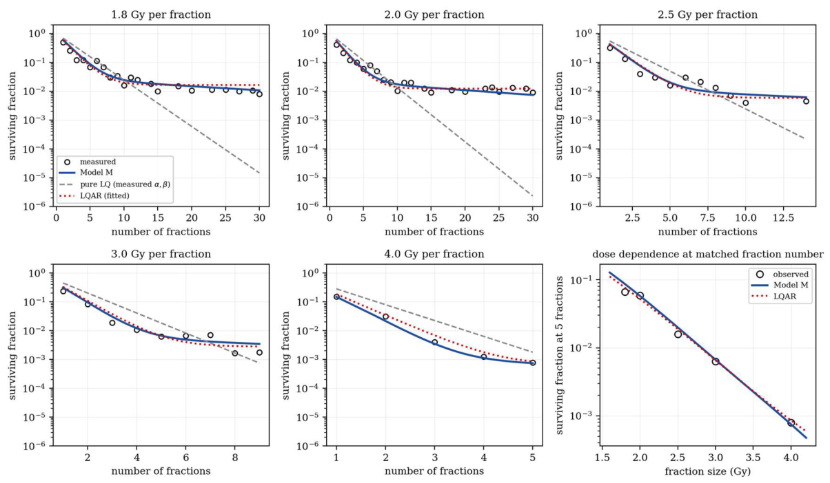
Two tests use quantities that did not enter the fit. First, the level at which each curve settles depends on fraction size in a way the model predicts without further parameters; regressing the settling level on L gives a slope of −2.84 ± 0.36 (R2 = 0.970), implying a gate accumulation of 1.84 fractions and excluding zero delay at p = 0.035. That value agrees with the fitted 1.75 although it was obtained from data held out of the fit. Second, comparison against the alternative in which a floor is added to the linear–quadratic expression by hand shows that the derived floor fits better in sample (root-mean-square residual 0.159 against 0.184), and that the alternative requires α = 0.220 Gy−1, an 89% increase over the measured single-dose value.
One clear negative is recorded. When whole fraction sizes are held out rather than individual points, the present model generalises slightly worse than the hand-added floor (0.211 against 0.198). The fit therefore establishes that a derived floor of the right shape and magnitude exists; it does not validate the mechanism. Nor are the parameters independently identifiable from a fractionation series at a single dose level, which is a structural property of the system rather than a deficiency of the data (Gutenkunst et al. 2007; Raue et al. 2009): varying fraction size is what identifies τγ, and r remains the least constrained parameter throughout.
An independent dataset both supports the construction and qualifies it. Gu et al. (2022) generated a tolerant population from a glioblastoma xenograft by successive irradiation, which confirms Axiom 1 directly rather than by inference. Two of their findings constrain the model. Colony-forming assays on successive populations return 45, 65 and 80 colonies from the same number of cells seeded, a 1.78-fold change with irradiation history alone; a surviving fraction normalised to plating efficiency therefore divides by a treatment-dependent quantity, and Theorem 1 holds for total clonogens and not for that ratio. This is a measurement requirement for the discriminating experiment, not a detail. They also report enhanced repair in the tolerant population, which is a departure from the assumption of Eq. 2 that repair is common to both compartments; if that difference is large the cancellation leading to Eq. 17 is perturbed and Theorem 1 weakens. We treat this as the principal open problem the construction faces.
7. Conventional Fractionation
Under daily fractions separated by 24 hours, with a repair half-time of 30 minutes and τσ = 30 min, the conditions of Section 4 are met and the system behaves as the map of Eq. 16. The clinical consequences of the asymptotic law then take their simplest form. At α = 0.127 Gy−1, β = 0.087 Gy−2, κ = 0.086, r = 0.063 and τγ = 1.75 d, fitted to fractionated clonogenic survival of U-251MG at five fraction sizes (Van den Berg et al. 2020), a course delivered with a front-loaded fraction-size profile exceeds a uniform course by a factor of 5.8 in surviving fraction at matched total dose and matched total dose-squared, where Eq. 1 predicts no difference at all. Reversing the same profile costs 1.97 in log-kill.
The placement of a sequential boost is the case where this matters most in current practice, because it is a discrete and re-orderable block of dose delivered late. An identical 15 Gy boost appended to a 60 Gy course buys 0.37 log-kill where Eq. 1 credits it with 5.82; the same dose delivered first buys 1.20. Section 7.3 works this through for glioblastoma, where the dose-response history is unusually complete.
The consolidation window is a consequence of τγ rather than a free parameter, and is therefore measurable independently of any fractionation fit: a priming–challenge series measures the same time constant that must reproduce the plateau. The cascade also predicts a smooth transition rather than a sharp threshold. The per-fraction log-kill falls from 0.602 at the first fraction through 0.586, 0.550 and 0.411 to 0.160 by the eighth, approaching rL = 0.038 thereafter, so a densely sampled early survival curve measures τγ directly.
The magnitude of the ordering effect depends on two parameters that are not tightly constrained: r has not been measured on a clonogenic endpoint, and τγ is pinned by a single dataset. We therefore give the results over the plausible ranges rather than at a point estimate. Table 2 gives the difference in log-kill between back-loaded and front-loaded delivery of an identical multiset of fraction sizes, at matched Σd and Σd2, so that Eq. 1 predicts exactly zero in every cell. The effect decreases monotonically with r, vanishing as r → 1 as Theorem 1 requires, and increases with the window, because a longer window leaves more of the course in the sensitive regime.
Table 3 converts this into the quantity a planner would use. Its pattern differs from Table 1 in a way that matters practically: the gain of front-loading over uniform delivery rises steeply with the window but varies only about two-fold across the whole range of r at short windows. The prescription is therefore robust to the parameter that is least well known, which is what allows a schedule to be specified from cohort values without measuring r in an individual.
Table 4 gives the boost result across the same range. An identical 15 Gy boost is placed either at the end of a 60 Gy course or before it; total dose and total dose-squared are identical between the two placements, so Eq. 1 returns the same survival for both at every r.
7.1. Consequences for the Planning Quantities
Biologically effective dose is defined so that log-kill is linear in dose, which is what makes it additive across a course and independent of order. Theorem 1 shows that linearity fails as soon as a second compartment exists. Two twenty-fraction courses ramping 3.0 → 1.0 Gy and 1.0 → 3.0 Gy have identical biologically effective dose to two decimal places, identical normal-tissue cost, and predicted surviving fractions differing 5.6-fold. The quantity remains exact for comparisons within a fixed delivery order, which is most of its clinical use, and that is why the deficiency is invisible until order is varied.
Tumour-control probability inherits the error and amplifies it, because control is exponential in surviving clonogens. At the fitted parameters a 60 Gy course in thirty fractions gives a surviving fraction of 1.29 × 10⁻² against the linear–quadratic value of 1.43 × 10⁻⁸, a discrepancy of nearly six orders of magnitude. A control probability computed from Eq. 1 therefore predicts near-certain control at clonogen burdens from 103 to 107 where the present construction predicts none. The direction is always the same: a linear–quadratic calculation is optimistic, and increasingly so as the burden rises.
Re-irradiation is the case where the reversion term of Eq. 6 becomes the governing quantity rather than a neglected one. Setting ρ > 0 and integrating in the absence of dose, the sensitive compartment recovers as 1 − e−ρt, so recovery to within five per cent of baseline takes ln20/ln2 = 4.32 reversion half-lives, independently of the half-life itself. For reported reversion half-lives of one, two and four weeks this is 30, 61 and 121 days. The prediction is that salvage efficacy rises monotonically with the interval since the first course and saturates at baseline, with a time constant matching an independently measurable reversion rate. Efficacy independent of interval, or recovering on a different timescale, refutes it.
7.2. Where the Benefit Is Largest
The results above are expressed in log-kill, which is what the construction computes. Converting to tumour control introduces the clonogen burden and the shape of the control curve, and the ranking reverses. Table 5 gives the absolute control gain from front-loading for a parameter set with intermediate baseline control (α = 0.25 Gy−1, β = 0.025 Gy−2, 70 Gy in 35 fractions, 107 clonogens). The log-kill gain falls monotonically with r, as Table 1 implies. The control gain does not: it is zero below r ≈ 0.5, peaks at +0.217 near r = 0.65, and decays above r ≈ 0.8.
The two extremes fail for opposite reasons. In a strongly tolerant tumour the schedule buys the most kill, but the tumour is far enough from control that a ten-fold reduction in survivors leaves control at zero, so the benefit expresses itself as delay rather than cure. In a weakly tolerant tumour control is already high and there is little tolerance to exploit. Only in the intermediate band do both conditions hold. The prediction is therefore that sequencing pays off most in moderately tolerant tumours with intermediate baseline control, which is the opposite of the expectation that a resistance mechanism should be targeted where resistance is greatest. It also implies that a disease in which the construction retrodicts observed failures need not be the disease in which it can be tested against a control endpoint.
7.3. Application to Glioblastoma
Glioblastoma provides a test because its dose–response history is unusually complete. Escalation above 60 Gy has been attempted repeatedly and has not improved survival, by external-beam escalation, radiosurgical boost, metabolically guided escalation, and intraoperative escalation (Nelson et al. 1988; Souhami et al. 2004; Chen et al. 2015; Laprie et al. 2024; Giordano et al. 2026), while 60 Gy in thirty fractions has remained standard for two decades (Stupp et al. 2005). Under Eq. 1 each additional 10 Gy at 2 Gy per fraction should buy 3.01 log-kill, which is not a marginal increment.
The asymptotic law removes the paradox, and the size of the effect is set by r rather than being qualitative. All of the escalated dose in those trials was delivered after the transfer was complete, where each increment is worth r times its nominal value: an additional 10 Gy buys 0.06 log-kill at r = 0.02, 0.19 at the fitted r = 0.063, 0.45 at r = 0.15 and 0.90 at r = 0.30, against 3.01 under Eq. 1. Across the plausible range the realised benefit is between two and thirty per cent of the expected one. The prediction that follows is specific: escalation delivered within the window would not be similarly devalued, and no escalation trial has front-loaded within the first week.
The same law accounts for a second observation. Extent of resection and residual tumour volume both predict survival, but residual volume is the stronger predictor when both are measured (Sanai et al. 2011; Grabowski et al. 2014; Li et al. 2016). This is what Section 5.2 requires: cytoreduction acts on the initial clonogen number and is undevalued, whereas dose acts through the hazard and is devalued by r, so their relative value is 1/r. A competing account exists and should be named. Osswald et al. (2015) describe a functional tumour-microtube network conferring collective resistance, which would also produce a volume-dependent effect; the two are separable because a collective mechanism predicts that the order effect depends on cell density whereas Axiom 1 does not, so the discriminating experiment of Section 13 should be run at two densities.
That separation can also be attempted in vivo, and on data already acquired. Because a collective mechanism makes the response of neighbouring sub-regions dynamically interdependent whereas Axiom 1 does not, the two accounts differ in a property that serial imaging can address: whether knowledge of a region’s neighbours improves prediction of its next state beyond its own history. A predictive index of that form has been developed for magnetic-resonance-guided radiotherapy, together with the result that any symmetric conservative coupling cancels exactly from the volume mean, so that mean apparent diffusion coefficient is structurally blind to it (Vaitheeswaran 2026b). We simulated both accounts under the dynamics of Eqs. 6 and 7 with a realistic dose distribution and imaging chain, and the index separates them: the area under the receiver operating characteristic for distinguishing cell-autonomous from collectively coupled tolerance is 0.95 for weak coupling and 1.00 for moderate and strong coupling, the two accounts being otherwise indistinguishable in both plateau shape and spatial heterogeneity.
Two conditions limit that test and are worth stating, because neither is obvious. The index reads apparent diffusion, which reports total cellularity and is dominated by the non-clonogenic majority, so an elevated value establishes that bulk response is coordinated rather than that clonogenic tolerance is; it therefore bears on Axiom 1 without measuring r. And the index depends strongly on the heterogeneity of the delivered dose. In our simulations of a purely cell-autonomous tumour with no coupling whatever, it returned 0.247 under a flat plan, 0.141 under a typical one and 0.024 under a steeply modulated one, a tenfold range driven by the plan alone and running in the counter-intuitive direction, because a steep gradient sustains the conditional heterogeneity against which the index is normalised. Any comparison between patients must therefore be matched on delivered dose heterogeneity as well as on acquisition protocol. The same dependence rules out using the index inside a feedback loop: reducing plan modulation in response to an elevated reading raises the reading further, so a controller of that form would be self-confirming.
One boundary should be stated plainly. Applied to clinical clonogen numbers the fitted parameters predict of order 106 survivors from 109 after 60 Gy in thirty fractions. For a tumour that radiotherapy does not sterilise this is qualitatively consistent with the dominance of local failure, but it means the construction is calibrated in a regime where radiotherapy fails, and taken with Table 4 it means glioblastoma is the right disease for the retrodictions above and the wrong one for a control endpoint.
7.4. Pulsed Schedules with Long Intervals
Axiom 6 neglects reversion because the interval between deliveries is short compared with the reversion half-life, which holds for daily fractionation. It does not hold for pulsed schedules. Personalised ultrafractionated stereotactic adaptive radiotherapy delivers a small number of large pulses separated by two to four weeks rather than daily fractions, with adaptation between pulses (Moore et al. 2021), and it is advocated principally on immunological grounds and for normal-tissue recovery (Peng et al. 2024; Rouf et al. 2024). In that regime the reversion term ρ of Eqs. 6 and 7 is no longer negligible, and the construction supplies a distinct rationale: a long interval allows the tolerant compartment to revert, so each pulse meets a partly resensitised population, and the schedule additionally incurs the transfer penalty only a few times rather than thirty.
Integrating Eqs. 6 and 7 with ρ > 0 gives the size and the shape of the effect. Retaining the fitted parameters and a reversion half-life of fourteen days, a five-pulse schedule at 12 Gy retains 27.0% of its linear–quadratic kill at a one-week interval and 30.9% at three weeks, against 30.5% for thirty daily 2 Gy fractions and 22.2% for a ten-fraction schedule at three-day intervals; a three-pulse schedule at 20 Gy retains 39.1%. Most of that advantage comes from delivering few fractions rather than from the intervals themselves. The interval effect is nonetheless real and has a specific shape: for the five-pulse schedule the gain over a no-reversion calculation is 10.3 log-kill at a 28-day interval with a seven-day reversion half-life, but only 2.6 log-kill if the half-life is 28 days. The prediction is therefore that benefit rises with interval and saturates at a few reversion half-lives rather than increasing without limit, and that the optimal interval tracks the same reversion rate that governs re-irradiation timing in Section 7.1.
This result is bounded in a way that should be stated rather than qualified afterwards. Equations 6 and 7 contain no repopulation term, so the construction can credit reversion during a long interval but cannot debit regrowth over the same period, and pulsed schedules spanning several months are precisely the regime in which that omission is largest. The figures above are therefore an upper bound on the benefit of lengthening the interval, and the construction cannot identify an optimal interval, which requires the competition between reversion and repopulation that it does not represent. Nor does it bear on the immunological rationale, since it contains no immune term; the mechanism described here is independent of that account and additive to it.
8. Dose Rate and Delivery Time
Two mechanisms reduce cell kill as delivery is prolonged at fixed dose, and both follow from Eqs. 2–3 rather than being imposed. Sublethal damage repairs during delivery, reducing the quadratic contribution through q in Eq. 2 (Dale 1985; Lea and Catcheside 1942). Independently, the cascade has time to act, so part of the transfer occurs while dose is still being delivered and later dose meets an already-converted population. The second mechanism is specific to a state-carrying kill law and is absent from Eq. 1 however it is repair-corrected.
The practical consequence is that delivery should be short. For a course of 35 fractions with the parameters of Section 7, distributing the control points of a volumetric-modulated arc plan across more arcs lowers predicted control monotonically, and compressing three arcs into one recovers 0.016 in absolute tumour control. Decomposing that figure by setting r = 1, which removes the transfer while leaving repair intact, attributes 0.0131 to repair and 0.0029 to the transfer. Prolonged delivery therefore costs about twenty per cent more than a repair-corrected calculation predicts, which is a modest quantitative correction to a known effect rather than a new effect.
Extrapolating to ultra-high dose rate does not extend the argument, and the derivation shows why. By Eq. 15 most of the transfer occurs after the beam is off, so shortening the beam-on time cannot suppress it: reducing delivery from one minute to 100 milliseconds changes predicted control by 0.007, against 0.080 from twelve arcs to one. Any benefit of ultra-high dose rate delivery must therefore act through normal-tissue sparing rather than through tumour transfer kinetics, and by relaxing the dose-squared budget that bounds front-loading it could act substantially: a fifteen per cent relaxation converts into about 0.24 in absolute control at these parameters.
9. Continuous Low-Dose-Rate Irradiation
Brachytherapy delivers dose continuously at a rate set by the source and the implant duration (Dale 1985). Equations 9 and 11 apply directly with Ḋ(t) constant. Table 6 gives the surviving fraction for 60 Gy delivered continuously over a range of durations, against thirty 2 Gy fractions computed in the same model.
Two features are worth stating. First, the model reproduces the classical dose-rate effect: prolonging delivery from one hour to thirty days raises survival by ten orders of magnitude, and most of that is sublethal repair. Second, the loss is larger than repair alone predicts. Repeating the calculation with r = 1, which removes the tolerance mechanism while leaving repair intact, gives −ln SF of 25.881 at 24 hours and 10.298 at seven days, against 8.116 and 4.346 with tolerance. The tolerance penalty is therefore 17.8 and 6.0 log-kill respectively: continuous low-dose-rate irradiation is penalised twice, once by repair and once by allowing the transfer time to act during delivery.
A specific equivalence follows. A seven-day continuous implant delivering 60 Gy gives −ln SF = 4.346 against 4.348 for thirty 2 Gy fractions, so the two are predicted to be biologically equivalent to three decimal places at these parameters. That equivalence is a property of this parameter set rather than a general law, but it is instructive: a repair-corrected LQ comparison of the same two schedules does not place them close (Dale 1985).
10. Radionuclide Therapy
Molecular radiotherapy delivers dose at a rate that decays with an effective half-life Teff combining physical decay and biological clearance, so Ḋ(t) = Ḋ0 e−λt with λ = ln2/Teff. Absorbed dose is the standard basis for prescribing and comparing such agents (Sgouros et al. 2020; Strigari et al. 2014), and we are not aware of an induced-tolerance mechanism having been considered in this setting. Equations 9 and 11 apply with Ḋ0 fixed by the prescribed absorbed dose.
Table 7.
Predicted log-kill for 60 Gy absorbed dose delivered with an exponentially decaying dose rate, against effective half-life. The fourth column repeats the calculation with r = 1, removing the tolerance mechanism but retaining repair; the fifth is the difference. Entries omitted where survival underflows.
Table 7.
Predicted log-kill for 60 Gy absorbed dose delivered with an exponentially decaying dose rate, against effective half-life. The fourth column repeats the calculation with r = 1, removing the tolerance mechanism but retaining repair; the fifth is the difference. Entries omitted where survival underflows.
| Effective half-life | Peak rate | −ln SF (model) | −ln SF (r = 1) | tolerance penalty |
|---|---|---|---|---|
| 0.1 d (2.4 h) | 0.29 Gy min−1 | 14.205 | — | — |
| 0.28 d (6.7 h) | 0.103 Gy min−1 | 10.024 | 29.352 | 19.328 |
| 1.0 d | 0.029 Gy min−1 | 6.455 | 14.024 | 7.569 |
| 2.8 d | 0.010 Gy min−1 | 4.681 | 9.938 | 5.257 |
| 8.0 d | 0.0036 Gy min−1 | 3.718 | 8.435 | 4.717 |
| 17.0 d | 0.0017 Gy min−1 | 3.357 | 8.004 | 4.648 |
| 30.0 d | 0.0010 Gy min−1 | 3.195 | 7.838 | 4.643 |
The prediction is monotone and steep: cell kill rises by more than four log-kill as the effective half-life falls from thirty days to six hours at identical absorbed dose, and by another four if it falls to 2.4 hours. Roughly half of that gradient is the conventional dose-rate effect and half is the tolerance penalty, which grows from 4.6 log-kill at thirty days to 19.3 at 6.7 hours in absolute terms.
Three consequences follow for the design of radionuclide therapy, and each is falsifiable. Absorbed dose alone is predicted to be an inadequate basis for comparing agents, because two agents delivering the same dose with different effective half-lives are predicted to differ by orders of magnitude in cell kill; this is already expected on repair grounds (Dale 1985) and the present construction makes the discrepancy larger. Shorter-lived isotopes and faster-clearing carriers should be favoured at matched absorbed dose. And fractionated administration, which is standard for several agents, distributes the delivery into separated cycles and therefore incurs the transfer penalty repeatedly; the model predicts that consolidating a course into fewer, larger administrations is preferable at matched absorbed dose, which parallels the front-loading conclusion of Section 7 and is testable in the same way.
We state one boundary explicitly. These calculations assume that the parameters fitted to acute external-beam fractionation apply unchanged at the dose rates of radionuclide therapy, which are three to four orders of magnitude lower. That assumption is untested, and the model itself gives a reason for caution: at low dose rates the cascade of Eq. 3 operates in a regime where σ never departs far from quasi-steady state, and the relation between κ and the observable transfer may differ. The magnitudes in Table 2 should therefore be read as a prediction of ordering and approximate scale, not as a dosimetric conversion.
11. Radiation Quality
The tolerance advantage of Eq. 17 depends on the tolerant compartment being harder to kill, and the tolerant state is reported to act in part through enhanced repair (Gu et al. 2022). Damage produced at high linear energy transfer (LET) is less repairable, which is the established reason the oxygen enhancement ratio falls with LET. If the advantage is repair-mediated, r should therefore rise toward unity as LET rises, and the schedule dependence of Section 7 should disappear. We parametrise this as 1 − r(ℓ) = (1 − r0) e−λ(ℓ − ℓ0), with ℓ0 the LET of the beam at which r0 was fitted, and treat it as a hypothesis to be refuted rather than an established coupling.
Table 8 gives the consequence across the clinical LET range. The schedule results of Section 7 are therefore a low-LET phenomenon, and the construction predicts that a carbon-ion beam abolishes the order effect entirely — a physical ablation of the mechanism requiring no inhibitor, and the cleanest available test of Theorem 1.
11.1. The Proton–Photon Asymmetry in Dose-Escalated Glioblastoma
A test of this coupling exists in a trial that escalated to the same prescribed dose by two radiation qualities within one protocol. In NRG-BN001, dose intensification to 75 Gy by photon intensity-modulated radiotherapy did not improve overall survival relative to 60 Gy, whereas the proton cohort at 75 Gy showed improved survival, with absolute gains of 6.8% at two years and 4.6% at three years, sufficient to trigger a phase III trial (Mehta et al. 2025). The trial’s own hypothesis for the asymmetry is reduced lymphopenia with protons.
The present construction predicts the same asymmetry from a tumour-cell mechanism. In the photon arm the escalated dose is delivered where each increment is worth r times its nominal value, so escalating 60 to 75 Gy buys 0.72 log-kill against the 7.78 that Eq. 1 predicts, nine per cent of the expected benefit, which is consistent with the observed absence of a survival difference. Under LET erosion the same escalation recovers progressively in the proton arm (Table 9).
The two accounts are separable, and we state the separation rather than claim priority. A lymphopenia mechanism is systemic: it should not depend on the tolerance of the tumour, and should operate at 60 Gy as well as at 75 Gy. A tolerance mechanism acts specifically on the escalated increment, is absent where r approaches unity, and predicts that the proton advantage scales with tumour tolerance. Collecting lymphocyte counts alongside a tolerance surrogate in the phase III trial would distinguish them.
The same coupling has a specific consequence for radionuclide therapy, because alpha-emitting agents combine high LET with low dose rate, and the two act in opposite directions in this model (Kim and Brechbiel 2012). Low dose rate gives the transfer time to act and should amplify the tolerance penalty; high LET erodes the advantage that penalty depends on. The second dominates: at an effective half-life of 2.8 days the tolerance penalty is 5.27 log-kill for a low-LET agent and 0.002 for a high-LET one. Alpha emitters are therefore predicted to escape the penalty almost entirely, and — the more distinctive prediction — to be insensitive to effective half-life, where beta emitters depend on it steeply (Figure 2c). That is a differential prediction rather than a claim about absolute potency, and it does not depend on the RBE model, which is uncertain at these LET values and which we do not attempt to calibrate.
12. Measuring the Tolerance Ratio In Vivo
Every clinical magnitude above scales with r, which has not been measured on a clonogenic endpoint. Recovering it from a response measurement is difficult for a structural reason: the observable is total clonogens, and the information distinguishing a tolerant from a sensitive population enters only through the difference between the two decay modes of Eq. 17, which is small when r is small and vanishes quadratically as r approaches unity. A single response trajectory is therefore a weak estimator of r, and a diffusion-weighted readout is weaker still, because it is sensitive to total cellularity including cells that are lethally damaged but not yet cleared, a compartment that dominates the signal during treatment.
Radionuclide therapy removes both obstacles at once, and does so without any additional measurement. Uptake is heterogeneous between tumour regions, so the dose rate differs between them while the isotope, the absorbed dose prescription and the tumour biology are shared; and that heterogeneity is quantified directly by the serial emission imaging already performed for dosimetry (Sgouros et al. 2020; Strigari et al. 2014). The dose-rate contrast is therefore a known covariate, and Section 10 shows that response depends steeply on it. A metabolic readout is required rather than a diffusion one, because it reports viable cells and does not saturate.
We computed the predicted contrast between a fast-clearing region (effective half-life 1 d) and a slow-clearing region (8 d) receiving equal absorbed dose. The difference in log standardised uptake at the end of treatment is 2.54 at r = 0.02, rising monotonically to 5.18 at r = 0.6, against a test–retest repeatability of about 0.12: the contrast is twenty to forty times the noise and is monotone in the quantity of interest. Setting r = 1 gives 5.86, so the tolerance mechanism accounts for between half and all of the departure from the repair-only prediction. Inverting the calibration with realistic noise recovers r with a correlation of 0.977 and a median absolute error of 0.027.
This is, to our knowledge, the only configuration in which the tolerance ratio is well identified in a patient, and it arises because the modality supplies its own covariate. The result carries the same caveat as Section 10: it assumes parameters fitted at acute external-beam dose rates apply at radionuclide dose rates, which is untested. It also assumes the tolerant compartment is metabolically distinguishable from the sensitive one, which is reported for drug-tolerant populations but with disagreement about direction (Hangauer et al. 2017; Russo et al. 2024); the calculation depends on the contrast existing, not on its sign.
13. Predictions
(P1) Blocking the transfer abolishes the order effect, provided repair is complete between deliveries. A matched-multiset contrast delivered in two orders differs in clonogenic survival, and the difference vanishes when the transfer is blocked. Section 5.1 imposes a condition that is easily overlooked: the interval must be long compared with the repair half-time, since incomplete repair produces order dependence at r = 1 (ratio 1.375 at one-hour intervals in our calculation). The contrast should also be run at two cell densities, to exclude a collective mechanism, and read as total clonogens rather than plating efficiency, since colony counts differ 1.78-fold between populations differing only in irradiation history (Gu et al. 2022).
(P2) The transfer completes after the beam is off. Equation 15 predicts that tolerance written by a fraction is realised during the following interval. A priming–challenge series with challenge intervals spanning minutes to days should therefore show protection developing after irradiation ends, with a time course set by τγ. The same parameter must reproduce the fractionation plateau, which is a consistency requirement linking two independent measurements.
(P3) The early survival curve is log-linear under induction and bends immediately under selection. Under selection, resistant cells are present from the outset and the local slope falls monotonically from the first fraction; under induction the curve begins at slope L and bends as γ accumulates. The cascade predicts a smooth transition rather than the sharp knee of the discrete formulation, and a densely sampled series over the first eight fractions distinguishes all three.
(P4) Continuous irradiation is penalised beyond repair. At matched total dose, continuous delivery should give less kill than a repair-corrected LQ calculation predicts, by an amount that grows with duration — 6.0 log-kill at seven days in our parameter set. Comparing a continuous implant with a fractionated course of matched dose, both measured clonogenically, isolates the excess.
(P5) Radionuclide kill depends steeply on effective half-life at matched absorbed dose. Two agents delivering equal absorbed dose with effective half-lives differing tenfold are predicted to differ by several log-kill (Table 2). This is testable in vitro with a decaying source or a source removed on a schedule, and it predicts that absorbed dose alone is an inadequate basis for comparing agents.
(P6) Boost timing changes outcome at fixed total dose. Moving an identical boost from the end of a course to the beginning improves kill, where Eq. 1 predicts no change. This is testable wherever a sequential boost is standard.
(P7) A persister-directed agent should be given late, not early. Because the transfer refills the tolerant compartment from a surviving sensitive pool, an agent that selectively kills tolerant cells gains 0.53 log-kill if given at the third fraction and 2.30 if given at the sixteenth or later, in our parameter set. Agents with this selectivity exist (Hangauer et al. 2017), so the prediction is testable with current compounds and concerns scheduling rather than choice of drug.
(P8) Carbon-ion irradiation abolishes the order effect. At carbon-ion LET the construction predicts r ≈ 1 and an order effect of zero. A matched-multiset order contrast delivered with carbon ions should return the null while the same contrast with photons in the same cell line returns 1.97 log-kill. The two arms differ only in beam quality, so no inhibitor is required. A non-zero carbon-ion effect refutes the repair-mediated account of tolerance without refuting the construction.
(P9) Alpha-emitting radiopharmaceuticals are insensitive to effective half-life; beta emitters are not. Section 11 predicts a tolerance penalty of 5.27 log-kill for a low-LET agent at 2.8 days effective half-life and 0.002 for a high-LET one, so log-kill should vary steeply with effective half-life for beta emitters and be nearly flat for alpha emitters (Figure 2c). This is a differential prediction, testable in vitro by varying clearance at matched absorbed dose for one agent of each class, and it is independent of the RBE model because it concerns the shape of the dependence rather than its absolute level.
14. Discussion
Two structural results carry the construction, and each is a property of the system rather than of its solution. The transfer cancels on adding Eqs. 6 and 7, so the ablation null of Theorem 1 is exact and independent of κ and of the functional form of the transfer; a prediction of exactly zero cannot be rescued by adjusting a parameter. The two-mode structure of Eq. 17 devalues late dose by r and yields the clinical corrections of Section 5.2 without further assumption.
One independent corroboration is worth recording, because it does not depend on the mechanism being correct. Alfonso and Berk (2019) derive a hypofractionation prescription from a continuous distribution of radiosensitivity re-weighted by differential killing, which is a pure selection mechanism and is incompatible with the induction assumed here. The same prescription follows from Eqs. 6 and 7 by induction. Two accounts that cannot both be right about the biology agree about the schedule, which means the prescription can be acted on without settling the mechanism, and that the schedule conclusion is more robust than the model that generates it.
Three features follow from working in continuous time and would be inaccessible to a law defined only between fractions. The consolidation window is a consequence of the gate time constant rather than a free parameter, and τγ is separately measurable from a priming–challenge series; this converts a fitted quantity into a testable identification and predicts a smooth rather than sharp transition. The order-independence corollary carries an explicit condition on repair, which is a design requirement for the discriminating experiment rather than a technicality (Dale 1986). And dose-rate dependence is derived from Eqs. 2–3 rather than assumed, which is what makes Section 8 to 12 possible.
Three application domains follow directly. Continuous low-dose-rate irradiation carries a tolerance penalty in addition to the repair penalty long recognised for protracted delivery (Dale 1985), a specific and measurable excess over the conventional calculation. Radionuclide therapy depends steeply on effective half-life at matched absorbed dose, which bears on agent selection and on whether absorbed dose suffices for comparison (Sgouros et al. 2020). And because high LET erodes the tolerance advantage while low dose rate amplifies it, alpha- and beta-emitting agents are predicted to differ not only in potency but in the shape of their dependence on effective half-life. The same modality supplies the dose-rate heterogeneity that makes r identifiable in vivo (Section 12).
The limitations are substantial. The parameters come from one cell line and one laboratory, from data digitised from published figures. The tolerance ratio r, which scales every clinical magnitude, has never been measured on a clonogenic endpoint, is uncertain by roughly a factor of eight, and is not constant, since Gu et al. (2022) show it deepening with successive irradiation. The cascade structure of Eq. 3 is the minimal choice that produces a delay, not a measured mechanism, and τσ and τγ are not independently identified by fractionation data; and the extension to the dose rates of radionuclide therapy assumes parameters fitted three to four orders of magnitude higher, which is untested. The model remains well-mixed and tumour-side, with no spatial structure, no immune term, and no normal-tissue claim, and it does not reproduce the clinical time factor, because accelerated repopulation is absent from Eqs. 6 and 7.
15. Conclusion
The discrete two-compartment map reproduces the fractionation plateau but contains no clock, and therefore cannot express dose rate, continuous delivery, or repair. The two structural results survive: the transfer cancels when the compartments are equally radiosensitive, so the ablation null holds; and late dose is devalued by the tolerance ratio, so the clinical corrections are unchanged.
Working in continuous time resolves a parameter and adds a condition. The consolidation window becomes a consequence of the gate time constant rather than a fitted quantity. The order-independence corollary requires complete inter-fraction repair, which is a design condition for the discriminating experiment. Statements about delivery time follow from the cascade rather than requiring an external timescale.
Two domains become accessible. Continuous low-dose-rate irradiation is predicted to lose more kill than repair alone accounts for, by six log-kill over a seven-day implant. Radionuclide therapy is predicted to depend steeply on effective half-life at matched absorbed dose, by more than four log-kill across the clinical range, which implies that absorbed dose is an insufficient basis for comparing agents. Both predictions are testable in vitro with existing methods, and neither could be stated in the discrete formulation.
Appendix. Notation
| Symbol | Meaning |
| Ns, Np | sensitive and tolerant clonogen populations |
| T | total clonogen population, Ns + Np |
| SF | surviving fraction |
| Ḋ(t), D(t) | dose rate (Gy min−1) and cumulative dose (Gy) |
| α, β | linear–quadratic coefficients (Gy−1, Gy−2) |
| h(t) | instantaneous lethal hazard, Eq. 2 |
| H(t) | cumulative lethality, ∫h dt |
| L | per-fraction lethality of an acute dose, αd + βd2 |
| q(t) | unrepaired sublethal damage (Lea–Catcheside memory), Eq. 2 |
| μ | sublethal repair rate, ln2/t½ʳᵉᵖ |
| σ(t) | fast damage signal, Eq. 3 |
| γ(t) | slow gate variable, Eq. 3 |
| τσ, τγ | signal and gate time constants |
| w(t) | transfer (write) rate, Eq. 4 |
| κ | transfer coefficient; total transfer per unit lethality, Eq. 5 |
| r | tolerance ratio; tolerant kill rate is r times sensitive |
| ρ | reversion rate (set to zero under A2) |
| Φ, Ψ | integrating-factor exponents, Eq. 8 |
| A, B, C | discrete per-fraction factors e−L, e−rL, e−κL |
| Teff | effective half-life of a radionuclide delivery |
References
- Alfonso, J.C.L.; Berk, L. Modeling the effect of intratumoral heterogeneity of radiosensitivity on tumor response over the course of fractionated radiation therapy. Radiat. Oncol. 2019, 14, 88. [Google Scholar] [CrossRef] [PubMed]
- Brenner, D.J. The linear-quadratic model is an appropriate methodology for determining isoeffective doses at large doses per fraction. Semin. Radiat. Oncol. 2008, 18(4), 234–239. [Google Scholar] [CrossRef] [PubMed]
- Chadwick, K.H.; Leenhouts, H.P. A molecular theory of cell survival. Phys. Med. Biol. 1973, 18(1), 78–87. [Google Scholar] [CrossRef] [PubMed]
- Chen, C.; Damek, D.; Gaspar, L.E.; et al. Phase I trial of hypofractionated intensity-modulated radiotherapy with temozolomide chemotherapy for patients with newly diagnosed glioblastoma multiforme. Int. J. Radiat. Oncol. Biol. Phys. 2015, 91(2), 269–275. [Google Scholar]
- Dale, R.G. The application of the linear-quadratic dose-effect equation to fractionated and protracted radiotherapy. Br. J. Radiol. 1985, 58(690), 515–528. [Google Scholar] [CrossRef] [PubMed]
- Dale, R.G. The application of the linear-quadratic model to fractionated radiotherapy when there is incomplete normal tissue recovery between fractions. Br. J. Radiol. 1986, 59(705), 919–927. [Google Scholar] [CrossRef] [PubMed]
- Forissier, V.; Rivera-Franco, M.M.; Cabeza-Segura, M.; et al. The LRP4/YAP axis drives the radiation-tolerant persister cell state in breast cancer. Theranostics 2025, 15(15), 7528–7546. [Google Scholar] [CrossRef] [PubMed]
- Fornalski, K.W.; Adamowski, L.; Dobrzynski, L.; et al. The radiation adaptive response and priming dose influence: the quantification of the Raper-Yonezawa effect and its three-parameter model for postradiation DNA lesions and mutations. Radiat. Environ. Biophys. 2022, 61(2), 221–239. [Google Scholar] [CrossRef] [PubMed]
- Fowler, J.F. The linear-quadratic formula and progress in fractionated radiotherapy. Br. J. Radiol. 1989, 62(740), 679–694. [Google Scholar] [CrossRef] [PubMed]
- Giordano, F.A.; Ganslandt, O.; Munter, M.W.; et al. Dose escalation with intraoperative radiotherapy in newly diagnosed glioblastoma (INTRAGO-II): an open-label, multicentre, randomised, controlled, phase 3 trial. Lancet Oncol. 2026, 27(7), 864–878. [Google Scholar] [CrossRef] [PubMed]
- Grabowski, M.M.; Recinos, P.F.; Nowacki, A.S.; et al. Residual tumor volume versus extent of resection: predictors of survival after surgery for glioblastoma. J. Neurosurg. 2014, 121(5), 1115–1123. [Google Scholar] [CrossRef] [PubMed]
- Gu, J.; Mu, N.; Jia, B.; et al. Targeting radiation-tolerant persister cells as a strategy for inhibiting radioresistance and recurrence in glioblastoma. Neuro-Oncology 2022, 24(7), 1056–1070. [Google Scholar] [CrossRef] [PubMed]
- Gutenkunst, R.N.; Waterfall, J.J.; Casey, F.P.; et al. Universally sloppy parameter sensitivities in systems biology models. PLoS Comput. Biol. 2007, 3(10), e189. [Google Scholar] [CrossRef] [PubMed]
- Hangauer, M.J.; Viswanathan, V.S.; Ryan, M.J.; et al. Drug-tolerant persister cancer cells are vulnerable to GPX4 inhibition. Nature 2017, 551(7679), 247–250. [Google Scholar] [CrossRef] [PubMed]
- Kellerer, A.M.; Rossi, H.H. The theory of dual radiation action. Curr. Top. Radiat. Res. Q. 1972, 8(2), 85–158. [Google Scholar]
- Kim, Y.S.; Brechbiel, M.W. An overview of targeted alpha therapy. Tumour Biol. 2012, 33(3), 573–590. [Google Scholar] [CrossRef] [PubMed]
- Kirkpatrick, J.P.; Meyer, J.J.; Marks, L.B. The linear-quadratic model is inappropriate to model high dose per fraction effects in radiosurgery. Semin. Radiat. Oncol. 2008, 18(4), 240–243. [Google Scholar] [CrossRef] [PubMed]
- Laprie, A.; Ken, S.; Filleron, T.; et al. Randomised phase III trial of metabolic imaging-guided dose escalation of radio-chemotherapy in patients with newly diagnosed glioblastoma (SPECTRO GLIO trial). Neuro-Oncology 2024, 26(1), 153–163. [Google Scholar] [CrossRef] [PubMed]
- Lea, D.E.; Catcheside, D.G. The mechanism of the induction by radiation of chromosome aberrations in Tradescantia. J. Genet. 1942, 44(2-3), 216–245. [Google Scholar] [CrossRef]
- Li, Y.M.; Suki, D.; Hess, K.; Sawaya, R. The influence of maximum safe resection of glioblastoma on survival in 1229 patients: can we do better than gross-total resection? J. Neurosurg. 2016, 124(4), 977–988. [Google Scholar] [CrossRef] [PubMed]
- McMahon, S.J. The linear quadratic model: usage, interpretation and challenges. Phys. Med. Biol. 2019, 64(1), 01TR01. [Google Scholar] [CrossRef] [PubMed]
- Mehta, M.P.; Pugh, S.; Mahajan, A.; et al. Signal-seeking P2R trial of proton or IMRT dose intensification in GBM: NRG-BN001. Int. J. Radiat. Oncol. Biol. Phys. 2025, 123(2S), LBA 15. [Google Scholar] [CrossRef]
- Moore, C.; Hsu, C.C.; Chen, W.M.; et al. Personalized ultrafractionated stereotactic adaptive radiotherapy (PULSAR) in preclinical models enhances single-agent immune checkpoint blockade. Int. J. Radiat. Oncol. Biol. Phys. 2021, 110(5), 1306–1316. [Google Scholar] [CrossRef] [PubMed]
- Nelson, D.F.; Diener-West, M.; Horton, J.; et al. Combined modality approach to treatment of malignant gliomas: re-evaluation of RTOG 7401/ECOG 1374 with long-term follow-up. NCI Monogr. 1988, 6, 279–284. [Google Scholar]
- Olivieri, G.; Bodycote, J.; Wolff, S. Adaptive response of human lymphocytes to low concentrations of radioactive thymidine. Science 1984, 223(4636), 594–597. [Google Scholar] [CrossRef] [PubMed]
- Osswald, M.; Jung, E.; Sahm, F.; et al. Brain tumour cells interconnect to a functional and resistant network. Nature 2015, 528(7580), 93–98. [Google Scholar] [CrossRef] [PubMed]
- Peng, H.; Moore, C.; Zhang, Y.; Saha, D.; Jiang, S.; Timmerman, R. An AI-based approach for modeling the synergy between radiotherapy and immunotherapy. Sci. Rep. 2024, 14(1), 8250. [Google Scholar] [CrossRef] [PubMed]
- Raue, A.; Kreutz, C.; Maiwald, T.; et al. Structural and practical identifiability analysis of partially observed dynamical models by exploiting the profile likelihood. Bioinformatics 2009, 25(15), 1923–1929. [Google Scholar] [CrossRef] [PubMed]
- Rouf, S.; Moore, C.; Saha, D.; et al. PULSAR effect: revealing potential synergies in combined radiation therapy and immunotherapy via differential equations. J. Theor. Biol. 2024, 599, 112026. [Google Scholar] [CrossRef] [PubMed]
- Russo, M.; Chen, M.; Mariella, E.; et al. Cancer drug-tolerant persister cells: from biological questions to clinical opportunities. Nat. Rev. Cancer 2024, 24(10), 694–717. [Google Scholar] [CrossRef] [PubMed]
- Sanai, N.; Polley, M.Y.; McDermott, M.W.; Parsa, A.T.; Berger, M.S. An extent of resection threshold for newly diagnosed glioblastomas. J. Neurosurg. 2011, 115(1), 3–8. [Google Scholar] [CrossRef] [PubMed]
- Sgouros, G.; Bodei, L.; McDevitt, M.R.; Nedrow, J.R. Radiopharmaceutical therapy in cancer: clinical advances and challenges. Nat. Rev. Drug Discov. 2020, 19(9), 589–608. [Google Scholar] [CrossRef] [PubMed]
- Sharma, S.V.; Lee, D.Y.; Li, B.; et al. A chromatin-mediated reversible drug-tolerant state in cancer cell subpopulations. Cell 2010, 141(1), 69–80. [Google Scholar] [CrossRef] [PubMed]
- Souhami, L.; Seiferheld, W.; Brachman, D.; et al. Randomized comparison of stereotactic radiosurgery followed by conventional radiotherapy with carmustine to conventional radiotherapy with carmustine for patients with glioblastoma multiforme: report of RTOG 93-05 protocol. Int. J. Radiat. Oncol. Biol. Phys. 2004, 60(3), 853–860. [Google Scholar] [CrossRef] [PubMed]
- Strigari, L.; Konijnenberg, M.; Chiesa, C.; et al. The evidence base for the use of internal dosimetry in the clinical practice of molecular radiotherapy. Eur. J. Nucl. Med. Mol. Imaging 2014, 41(10), 1976–1988. [Google Scholar] [CrossRef] [PubMed]
- Stupp, R.; Mason, W.P.; van den Bent, M.J.; et al. Radiotherapy plus concomitant and adjuvant temozolomide for glioblastoma. N. Engl. J. Med. 2005, 352(10), 987–996. [Google Scholar] [CrossRef] [PubMed]
- Vaitheeswaran, R. A predictive framework for detecting non-independent tumour dynamics in longitudinal MR-guided radiotherapy; Preprints.org, 2026b. [Google Scholar]
- Van den Berg, J.; Castricum, K.C.M.; Meel, M.H.; et al. Development of transient radioresistance during fractionated irradiation in vitro. Radiother. Oncol. 2020, 148, 107–114. [Google Scholar] [CrossRef] [PubMed]
- Withers, H.R. The four Rs of radiotherapy. Adv. Radiat. Biol. 1975, 5, 241–271. [Google Scholar] [CrossRef]
- Withers, H.R.; Taylor, J.M.; Maciejewski, B. The hazard of accelerated tumor clonogen repopulation during radiotherapy. Acta Oncol. 1988, 27(2), 131–146. [Google Scholar] [CrossRef] [PubMed]
- Zhao, Y.; Li, D.; Zhou, Y.; et al. Cancer cells enter an adaptive persistence to survive radiotherapy and repopulate the tumor. Adv. Sci. 2023, 10(8), 2204177. [Google Scholar] [CrossRef] [PubMed]
Figure 2.
Continuous delivery. (a) Log-kill for 60 Gy delivered continuously against implant duration, with and without the tolerance mechanism; the shaded band is the tolerance penalty, and the dotted line is thirty 2 Gy fractions computed in the same model. (b) The same for an exponentially decaying dose rate, against effective half-life. (c) Log-kill normalised to the shortest half-life, for low-LET (beta) and high-LET (alpha) delivery: erosion of the tolerance advantage at high LET removes the dependence on effective half-life.
Figure 2.
Continuous delivery. (a) Log-kill for 60 Gy delivered continuously against implant duration, with and without the tolerance mechanism; the shaded band is the tolerance penalty, and the dotted line is thirty 2 Gy fractions computed in the same model. (b) The same for an exponentially decaying dose rate, against effective half-life. (c) Log-kill normalised to the shortest half-life, for low-LET (beta) and high-LET (alpha) delivery: erosion of the tolerance advantage at high LET removes the dependence on effective half-life.
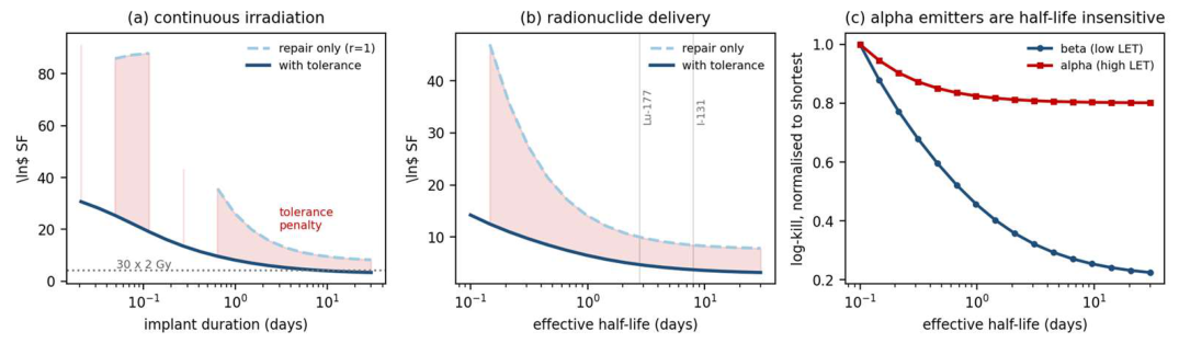
Table 2.
Order effect in log-kill (back-loaded minus front-loaded) for an identical multiset of fraction sizes at matched total dose and total dose-squared, across the plausible ranges of the tolerance ratio and the gate accumulation window. Equation 1 predicts identically zero everywhere in this table.
Table 2.
Order effect in log-kill (back-loaded minus front-loaded) for an identical multiset of fraction sizes at matched total dose and total dose-squared, across the plausible ranges of the tolerance ratio and the gate accumulation window. Equation 1 predicts identically zero everywhere in this table.
| window \ r | 0.02 | 0.063 | 0.15 | 0.30 | 0.50 | 0.70 | 0.85 |
|---|---|---|---|---|---|---|---|
| 0.5 fx | 0.840 | 0.794 | 0.704 | 0.553 | 0.362 | 0.185 | 0.069 |
| 1.75 fx | 2.065 | 1.968 | 1.773 | 1.439 | 1.001 | 0.573 | 0.259 |
| 4 fx | 4.343 | 4.150 | 3.758 | 3.084 | 2.186 | 1.280 | 0.589 |
| 8 fx | 5.676 | 5.425 | 4.918 | 4.041 | 2.863 | 1.652 | 0.737 |
| 12 fx | 6.153 | 5.881 | 5.329 | 4.370 | 3.064 | 1.713 | 0.736 |
Table 3.
Surviving-fraction gain of a front-loaded course over uniform 2 Gy delivery at matched total dose (60 Gy) and matched total dose-squared. Equation 1 predicts 1.00 in every cell. The decline from 8 to 12 fractions occurs because a window longer than the front-loading budget leaves dose to be spent after the schedule has flattened.
Table 3.
Surviving-fraction gain of a front-loaded course over uniform 2 Gy delivery at matched total dose (60 Gy) and matched total dose-squared. Equation 1 predicts 1.00 in every cell. The decline from 8 to 12 fractions occurs because a window longer than the front-loading budget leaves dose to be spent after the schedule has flattened.
| window \ r | 0.02 | 0.063 | 0.15 | 0.30 | 0.50 | 0.70 | 0.85 |
|---|---|---|---|---|---|---|---|
| 0.5 fx | 2.13 | 2.14 | 2.17 | 2.22 | 2.31 | 2.44 | 2.59 |
| 1.75 fx | 6.03 | 5.80 | 5.36 | 4.70 | 3.97 | 3.39 | 3.06 |
| 4 fx | 33.71 | 30.16 | 24.08 | 16.36 | 9.79 | 5.83 | 3.94 |
| 8 fx | 62.09 | 54.17 | 41.10 | 25.50 | 13.39 | 6.87 | 4.18 |
| 12 fx | 51.24 | 45.07 | 34.72 | 22.03 | 11.76 | 6.14 | 3.92 |
Table 4.
Surviving fraction for two placements of an identical 15 Gy boost within a 75 Gy course. Total dose and total dose-squared are identical between the two columns, so Eq. 1 returns the same value for both at every r.
Table 4.
Surviving fraction for two placements of an identical 15 Gy boost within a 75 Gy course. Total dose and total dose-squared are identical between the two columns, so Eq. 1 returns the same value for both at every r.
| r | boost at end | boost at start | gain from moving it early |
|---|---|---|---|
| 0.02 | 2.03 × 10⁻² | 8.51 × 10⁻³ | 2.39× |
| 0.063 | 7.89 × 10⁻³ | 3.44 × 10⁻³ | 2.29× |
| 0.15 | 1.17 × 10⁻³ | 5.54 × 10⁻⁴ | 2.11× |
| 0.30 | 4.46 × 10⁻⁵ | 2.43 × 10⁻⁵ | 1.84× |
| 0.50 | 6.07 × 10⁻⁷ | 3.97 × 10⁻⁷ | 1.53× |
| 0.70 | 9.33 × 10⁻⁹ | 7.32 × 10⁻⁹ | 1.28× |
| 0.85 | 4.90 × 10⁻¹⁰ | 4.38 × 10⁻¹⁰ | 1.12× |
Table 5.
Absolute tumour-control gain from front-loading against the tolerance ratio. The control gain is non-monotonic although the log-kill gain is monotone.
Table 5.
Absolute tumour-control gain from front-loading against the tolerance ratio. The control gain is non-monotonic although the log-kill gain is monotone.
| r | TCP, uniform | TCP, front-loaded | TCP gain | log-kill gain |
|---|---|---|---|---|
| 0.02 | 0.000 | 0.000 | +0.000 | 1.20 |
| 0.30 | 0.000 | 0.000 | +0.000 | 0.93 |
| 0.50 | 0.000 | 0.000 | +0.000 | 0.75 |
| 0.60 | 0.016 | 0.117 | +0.102 | 0.66 |
| 0.65 | 0.184 | 0.401 | +0.217 | 0.62 |
| 0.70 | 0.496 | 0.674 | +0.178 | 0.57 |
| 0.80 | 0.880 | 0.925 | +0.045 | 0.49 |
| 0.90 | 0.973 | 0.982 | +0.009 | 0.41 |
Table 6.
Predicted survival for 60 Gy delivered continuously over the stated duration, computed from Eqs. 2–3 and 6–7 with τσ = 30 min, τγ = 1.75 d, repair half-time 30 min, r = 0.063 and κ = 0.086. The fractionated row uses the same parameters.
Table 6.
Predicted survival for 60 Gy delivered continuously over the stated duration, computed from Eqs. 2–3 and 6–7 with τσ = 30 min, τγ = 1.75 d, repair half-time 30 min, r = 0.063 and κ = 0.086. The fractionated row uses the same parameters.
| Delivery | Dose rate | Surviving fraction | −ln SF |
|---|---|---|---|
| 30 × 2 Gy fractions | — | 1.29 × 10⁻² | 4.348 |
| continuous, 1 h | 1.00 Gy min−1 | 3.08 × 10⁻¹² | 26.505 |
| continuous, 24 h | 0.042 Gy min−1 | 2.99 × 10⁻⁴ | 8.116 |
| continuous, 3 d | 0.014 Gy min−1 | 4.01 × 10⁻³ | 5.519 |
| continuous, 7 d | 0.006 Gy min−1 | 1.30 × 10⁻² | 4.346 |
| continuous, 30 d | 0.0014 Gy min−1 | 3.46 × 10⁻² | 3.364 |
Table 8.
Tolerance ratio, order effect (log-kill at matched Σd and Σd2) and front-loading gain across the clinical range of linear energy transfer, under the erosion model with λ = 0.12 μm keV−1. LET values are indicative of the stated depth rather than exact.
Table 8.
Tolerance ratio, order effect (log-kill at matched Σd and Σd2) and front-loading gain across the clinical range of linear energy transfer, under the erosion model with λ = 0.12 μm keV−1. LET values are indicative of the stated depth rather than exact.
| Modality and depth | LET | r | order effect | front-load gain |
|---|---|---|---|---|
| photons (reference) | 1 | 0.063 | 1.968 | 5.80× |
| protons, entrance | 2 | 0.169 | 1.711 | 5.15× |
| protons, mid-SOBP | 5 | 0.420 | 1.124 | 3.83× |
| protons, distal edge | 10 | 0.682 | 0.553 | 2.68× |
| protons, distal fall-off | 20 | 0.904 | 0.126 | 1.67× |
| carbon ions, plateau | 40 | 0.991 | 0.011 | 1.24× |
| carbon ions, SOBP | 80 | 0.9999 | 0.000 | 1.23× |
Table 9.
Log-kill gained by escalating 60 Gy to 75 Gy in thirty fractions at the fitted parameters. The photon row uses the fitted r; proton rows apply the erosion model anchored at the photon reference. Equation 1 predicts 7.777 for every row.
Table 9.
Log-kill gained by escalating 60 Gy to 75 Gy in thirty fractions at the fitted parameters. The photon row uses the fitted r; proton rows apply the erosion model anchored at the photon reference. Equation 1 predicts 7.777 for every row.
| Arm | LET | r | log-kill gain, 60 → 75 Gy | fraction of LQ |
|---|---|---|---|---|
| linear–quadratic expectation | — | — | 7.777 | 100% |
| photon | 1 | 0.063 | 0.719 | 9% |
| proton, low-LET target | 3 | 0.263 | 2.305 | 30% |
| proton, mid-SOBP | 5 | 0.420 | 3.389 | 44% |
| proton, target-average | 7 | 0.544 | 4.202 | 54% |
| proton, distal-weighted | 10 | 0.682 | 5.042 | 65% |
Disclaimer/Publisher’s Note: The statements, opinions and data contained in all publications are solely those of the individual author(s) and contributor(s) and not of MDPI and/or the editor(s). MDPI and/or the editor(s) disclaim responsibility for any injury to people or property resulting from any ideas, methods, instructions or products referred to in the content. |
© 2026 by the authors. Licensee MDPI, Basel, Switzerland. This article is an open access article distributed under the terms and conditions of the Creative Commons Attribution (CC BY) license (http://creativecommons.org/licenses/by/4.0/).
Copyright: This open access article is published under a Creative Commons CC BY 4.0 license, which permit the free download, distribution, and reuse, provided that the author and preprint are cited in any reuse.