

Submitted:
11 August 2026
Posted:
12 August 2026
You are already at the latest version
Abstract
Thermodynamic reasoning has entered nonlinear optics along three routes—wave-turbulence kinetics, the equilibrium thermodynamics of highly multimoded systems, and the statistical mechanics of mode locking—but in each the modal basis or coarse-graining cutoff is specified externally, by a waveguide, a spectral window, or a cavity bandwidth. This review asks what survives when the object is a strongly chirped dissipative soliton of the complex cubic–quintic Ginzburg–Landau equation, a structure that exists only because energy flows through it. The mechanism that localizes such a pulse also bounds its spectrum, separating the correlation function into a graining scale set by the spectral cutoff and a collective scale set by the spectral core. Their ratio is selected by the dynamics rather than imposed, and closed-form adiabatic spectra in both dispersion regimes compress the parameter space onto a single master diagram carrying a shape entropy, an internal energy, and a continuation-dependent energy–entropy slope. Dissipative soliton resonance is read as spectral core narrowing, intrinsic in normal dispersion and conditional in anomalous dispersion. We state precisely where the borrowed vocabulary becomes strained: a deterministic pulse remains first-order coherent, so the scale ratio is not yet a count of statistical degrees of freedom, and the promotion requires an ensemble-coherence calibration that is specified but not assumed. The result is a falsifiable framework for dissipative-soliton coherence, energy scaling, and stability, with experimental signatures and design criteria for chirped-pulse oscillators.
Keywords:
dissipative soliton
; complex cubic–quintic Ginzburg–Landau equation
; dissipative soliton resonance
; spectral scale separation
; thermodynamic-like indicators
; optical wave turbulence
; Rayleigh–Jeans spectrum
; correlation scales
; energy–entropy slope
; chirped-pulse oscillator
1. Introduction
The most effective way to extract a large pulse energy directly from a mode-locked oscillator is not to make the pulse more intense but to make it longer. In an all-normal-dispersion fiber laser [1] or a solid-state chirped-pulse oscillator [2,3], the intracavity pulse is strongly chirped: dispersion and self-phase modulation stretch it in time, its peak power stays below the level at which nonlinearity destroys it, and the compression of the strongly chirped pulse is performed outside the cavity. Pulse stretching enables energy scaling while limiting the intracavity peak power. Pushed to its limit, this mechanism is dissipative soliton resonance (DSR), a region of parameter space in which the stationary branch admits unbounded energy scaling while its peak power and spectral width remain bounded—a statement about a family of solutions, not a guarantee that every member of it is stable [4,5,6]. Real oscillators do not deliver an infinite energy: they reach a finite maximum, beyond which the single-pulse becomes unstable. Multipulsing is one route by which it does so. Additionally, continuous-wave breakthrough, breathing and period-doubling, Q-switched mode locking, noise-like operation, Raman-induced instabilities, dispersive-wave destabilization and outright loss of mode locking all terminate energy scaling in real oscillators, and which channel is reached first depends on the concrete situation. This paper is organized around one question: within the model adopted below, what fixes that energy scalability maximum?
The question is not fully answered by the existence and stability analysis that produced DSR in the first place. In the modeled regimes of interest here—and we emphasize some regimes, since the anomalous-dispersion chirped branch is demonstrably not uniformly stable (Section 5.2)—a linearly stable single-pulse attractor coexists with a linearly stable multipulse one, and the multipulse state is the one the oscillator is observed to settle into. Which state is reached is fixed by basin volumes, by the perturbation history, by noise-driven transition rates, and by how the operating point was approached—not by any minimization principle established so far. Selection between coexisting attractors is not decided by linear stability. It is decided by which state a noisy, driven dynamics finds and holds, and that is a statistical question. It is the reason for reaching, as several authors have, for the language of thermodynamics, and the reason is that this language has to be examined carefully before it is used, because the object to which it is being applied is a single pulse, not an ensemble.
What makes a single pulse a candidate thermodynamic system is the way in which its solution family is organized. A conservative soliton is not, of course, a single solution either: the cubic nonlinear Schrödinger equation possesses continuous families parameterized by amplitude, width, frequency, velocity, position, and phase [7,8], and ensembles of such solitons carry a well-developed statistical mechanics of their own in soliton-gas theory [9,10]. The difference is one of selection rather than of counting. In the conservative case, the family is generated by the invariances of the equation together with its conserved quantities—some directions, such as position and global phase, are genuine symmetry orbits, while amplitude labels physically distinct solitons—and nothing in the dynamics prefers one member over another. In the dissipative case, the gain–loss balance selects members. At one fixed set of coefficients, a stable DS is normally an isolated attractor, possibly coexisting with others in separate basins. The energies and durations that make up the “family” are traced out by continuation in a control parameter, not chosen freely at unchanged coefficients [11,12,13]. Four distinct objects are kept apart throughout: an isolated attractor at a specified operating point; a continued branch as a coefficient is varied; coexistence of attractors in different basins at one point; and, once noise is admitted, branch occupancies and transition rates between them. It is the last—selection among coexisting attractors—that calls for a statistical criterion, and it is a question about basins and transition rates, not about the existence of a family.
In the strongly chirped regime, that energy flow produces the soliton internal structure. The chirp makes the pulse phase-inhomogeneous, so that energy is injected near the spectral center, where the gain exceeds the spectral loss, and drained at the wings, where the chirp has carried the instantaneous frequency away from the filter maximum. It is essential to state what this does and does not establish. A strong chirp generates deterministic internal frequency–time structure and, with it, a finite correlation width. It does not by itself generate statistical incoherence, since a deterministic field of arbitrary spectrum and arbitrary temporal dependence remains first-order coherent in Glauber’s sense [14,15], and its mutual-coherence kernel factorizes. Partial coherence, and with it a nontrivial spectrum of coherent modes, enters only through an ensemble: quantum and technical noise, shot-to-shot variability, slowly fluctuating saturable gain, or unresolved degrees of freedom. The program of this paper is therefore conditional. We mark it as such throughout: the chirp supplies two deterministic scales, and whether their ratio is also related to a count of statistically independent internal degrees of freedom—as it would be for a genuinely incoherent structure in the sense established in kinetic theory [16,17]—is a hypothesis to be tested against a defined ensemble, not a consequence of the chirp. As Section 4.3 shows, the ratio in question is in fact smaller than unity over much of the operating diagram, so it cannot be a mode count in the literal sense at all. The testable statement is a connection of the soliton destabilization statistics with the behavior of the soliton internal states of freedom treated thermodynamically.
Thermodynamic language has already been brought into nonlinear optics with considerable success, along three largely independent routes. Weak-turbulence kinetics supplies an irreversible relaxation towards a Rayleigh–Jeans spectrum, an H-theorem, and condensation of the wave energy into the lowest modes [16,17,18,19]. The equilibrium thermodynamics of highly multimoded systems supplies an extensive entropy, an equation of state, and Rayleigh–Jeans thermalization in a finite guided-mode set [20,21,22]. Negative-temperature Rayleigh–Jeans equilibrium states have subsequently been observed directly in multimode optical fibre [23], while related negative-optical-temperature thermodynamic processes have been explored on other photonic platforms [24,25]. The noise-driven statistical mechanics of mode locking supplies a Gibbs measure over cavity modes and treats pulse formation as a first-order phase transition [26,27,28]. These three routes are set out in Section 3, because the framework developed here is most defined by the contrast with them. What they share is decisive: in each, the modal basis or coarse-graining cutoff is a property of the setup—an ultraviolet cutoff imposed by discretization or by a finite band, the number of guided modes fixed by the fiber geometry, the coarse-graining correlation scale by the spectral filter—and that basis, as distinct from the occupations defined on it, does not respond to the energy stored in the field. It is the “volume” variable of those theories.
For a strongly chirped DS, it does respond, and that is the hypothesis on which this paper turns. The mechanism that localizes the pulse also bounds its spectrum: resonance of the soliton wavenumber with the linear dispersive waves fixes a cutoff frequency, and the requirement of non-negative power truncates the spectrum there, leaving a Lorentzian of width cut off at —a Rayleigh–Jeans distribution with an effective chemical potential (a spectral-shape parameter occupying the algebraic position of a chemical potential; see Section 4.3) [29,30,31]. A bounded spectrum generates two scales in the field autocorrelation rather than one: a short graining scale set by the spectral edge and a long collective scale set by the spectral core. Their ratio
is the spectral scale-separation index on which everything below is built. r is used as the primary variable, and the relation between the two is written as ∼ rather than as an equality: the factor relating them is a width convention, comparing the first zero of a sinc kernel with the decay length of an exponential. What is convention-free is the range and the ordering: on the unscalable branch (Sec. 2.2), where the two spectral scales merge and the deterministic pulse becomes effectively a single-scale spectral structure; on the fidelity curve (Sec. 2.2); and in the resonance limit (Sec. 5). Since the participation number of an ensemble coherence operator satisfies by construction, a useful calibration against it would be expected to approach the one-mode limit as , where the two spectral scales merge, and to be reproducibly nondecreasing over the tested range of r. Whether remains unbounded as —the limit that corresponds to dissipative soliton resonance—is not fixed by the deterministic scale separation and must be determined from the ensemble: finite detector bandwidth, gain correlations, noise statistics and the alignment protocol may in principle cause the participation number to saturate. The testable proposition is stated in Section 4.3: , computed from a defined ensemble, is a reproducible monotone function . What is established without that step is structural: r occupies the place that the mode number occupies in conservative multimode thermodynamics. Still, it is generated by the solution rather than imposed on it, and it depends on the operating point and on the energy.
Everything that follows is a consequence of that displacement, and the chain is short enough to state here. First, DSR admits a thermodynamic-like spectral interpretation within the reduced adiabatic description: it is the limit in which the chemical-potential-like shape parameter vanishes at finite cutoff—a spectral condensation—and the energy is harvested purely by temporal stretching (Section 5). Whether that limit is reachable turns out to differ between the two dispersion regimes: in normal dispersion it follows from the admissibility constraints of the chirped branch. It is intrinsic to it, whereas in anomalous dispersion it is conditional on a geometric intersection that translates into a threshold on the quintic phase nonlinearity [32]. Second, this narrowing raises the shape indicator (treated as entropy) of the normalized spectrum, because the two scales decouple and the scale separation widens instead of power being redistributed over a fixed set of states. It contrasts with the standard Bose–Einstein picture. However, the contrast is a statement about the shape functional and not about the total entropy referred to a fixed frequency bin, which also carries a falling scale term (Section 6.1). Third, along the specified isogain continuation and beyond a threshold energy, the internal-energy proxy passes through a maximum while the chosen entropy indicator continues to rise, so the directional energy–entropy slope changes sign —formally the mirror image of the textbook bounded-spectrum case, in which the entropy has an interior maximum and the temperature passes through infinity rather than through zero (Section 6.3). This is a property of the continuation and of the adopted diagnostics, not an equilibrium absolute temperature. Fourth, at some energy, the additive entropy proxy of a multipulse complex carrying the same total energy at the same net gain may exceed that of its single-pulse counterpart, which we advance as a candidate selection rule for fragmentation [33,34]. Because the pulses of such a complex share a single gain reservoir, the additivity on which the comparison rests is an assumption to be tested against transition statistics rather than granted. On this reading, and in normal dispersion, the ceiling on energy scaling need not be a loss of existence or of linear stability: it may be entropic in origin and arrive before the solution ceases to exist. That is a proposal, not a result—it presupposes the ensemble of Section 4.3 and the additivity of Section 6.4—and it does not transpose to anomalous dispersion: along the continuation examined there, the adopted indicators show neither an entropy turnover nor a sign reversal, and, independently, the available finite-time noisy linearized scan displays a one-sided accessibility boundary inside the algebraic existence region, whose status as the asymptotic energy-limiting mechanism remains open (Section 6.5 and 6.6). Neither claim excludes the other channels listed above; the model addresses one of them.
This is a critical synthesis of that framework rather than a survey of DSs, for which comprehensive accounts exist [11,12], and rather than a report of a completed thermodynamics. Much of what follows was developed in three recent papers [31,32,34]. The present purpose is to state that framework in one place, to separate what it establishes from what it assumes, and to specify the calculations and measurements that would decide the difference. Several things are attempted here that the primary papers do not. The adiabatic theories of normal and anomalous dispersion are brought onto a single master diagram, so that the two resonance mechanisms can be compared rather than merely juxtaposed. The scale-separation index is confronted with the definition it would have to satisfy—the participation ratio of a Karhunen–Loève decomposition of an ensemble coherence kernel [35,36]—together with an explicit statement of the assumptions that definition requires and of the ones it is not yet known to satisfy [37]. The choice of entropy functional is made explicitly, the state-dependent scale term discarded in earlier treatments is restored, and the consequences for the entropy ceiling and for the temperature are recomputed. The correspondence with driven-open condensates is put on a term-by-term basis, with the reservoir, noise, and geometry assumptions under which the reduction holds stated rather than suppressed, its sign convention fixed once, and the chirped DS located within the family of dissipative condensate models according to what each member conserves and what each minimizes [38,39,40]. A density-of-states argument is used to separate the part of the divergence between DS spectral condensation and Bose–Einstein condensation that is kinematic from the part that is genuinely dissipative in origin.
Much of what follows was developed in three recent papers [31,32,34]. The present purpose is to state that framework in one place, to separate what it establishes from what it assumes, and to specify the calculations and measurements that would decide the difference.
The scope is correspondingly well-defined, and five limitations should be stated at the outset rather than discovered later. (i) The analysis is confined to the -dimensional complex cubic–quintic Ginzburg–Landau equation in its strongly chirped regime, where the reactive dispersion and nonlinear phase terms dominate the corresponding dissipative corrections sufficiently for the adiabatic strong-chirp reduction to remain controlled. Outside that regime, the closed-form spectra, and with them the whole apparatus, are unavailable. (ii) The statistical object is not yet secured. All spectra used below are those of a single deterministic solution, whose coherence kernel is of rank one. The identification of with a coherent-mode participation number presupposes an ensemble that is defined here (Section 4.3) but not yet constructed, and the eigenvalue calculation that would test the identification has not been performed. (iii) The treatment is mean-field, and the modal weights that would enter any participation number are known to be closure-dependent [37]. (iv) The differential entropy of a continuous spectrum depends on the reference measure. We therefore fix a state-independent frequency bin, retain the scale term that this makes explicit, and report which conclusions survive its restoration and which do not (Section 6.1). (v) Because the system is genuinely out of equilibrium, the entropy, temperature, and free energy defined below are thermodynamic-like indicators evaluated along a named continuation path rather than state functions of an equilibrium theory: is a directional slope whose path independence has not been demonstrated, free-energy minimization does not select the stable state, and the entropy and internal-energy crossings acquire predictive content only once they are corroborated by direct dynamical simulation. Making the status of these quantities explicit, rather than assuming it, is one of the tasks of this paper. Table 1 summarizes its claim by claim, and the labels used there are used again in the conclusions.
The paper is organized as follows. Section 2 sets out the model and the adiabatic theory, derives the spectra in both dispersion regimes, and constructs the master diagram on which the rest of the argument is conducted. Section 3 reviews the three traditions of optical thermodynamics and isolates the assumption they share. Section 4 applies them to the chirped DS and finds that precisely that assumption fails: it establishes the two spectral scales, shows why a Schrödinger soliton has only one, defines the scale-separation index, and states what would have to be computed before that index could be called a count. Section 5 reformulates DSR in these terms and separates the intrinsic from the conditional resonance. Section 6 defines the thermodynamic-like indicators, fixes the conventions they depend on, and examines the limits of energy scaling—growth of the shape indicator, the turnover of the differential entropy, the sign reversal of the energy–entropy slope, and fragmentation. Section 7 assesses the analogies with wave turbulence, with the noise-driven theory of mode locking, and with driven-open condensates, stating what each explains and where each fails. Section 8 collects the conclusions, the open questions, and the outlook.
2. The Chirped Dissipative Soliton and Its Adiabatic Theory
The whole of what follows is derived from a closed-form asymptotic solution for the strongly chirped DS, so that solution is set out first. The order is deliberate. Every descriptor introduced later—the two spectral scales, the scale-separation index, the entropy-like functionals—is computed from a particular deterministic solution, and none can be formulated until that solution is available in the spectral domain. That is a statement about where the descriptors come from, not a claim that they are statistical. Statistical statements require an ensemble, which is supplied nowhere in this paper and is specified as future work in Section 4.3. This section supplies the solution: the model and the routes available for solving it (Section 2.1), the adiabatic construction itself (Section 2.2), and the parametric space which it generates (Section 2.3).
Three conventions are fixed here and used throughout.
Fourier transform:, . The spectral power is , the energy , and linear waves are written as . Dimensions:z is a propagation length (for a cavity map, a round-trip number, so that all below are per round trip) and t a retarded time, so that Table 2 applies. Provenance: equations reproduced from the primary papers, corrected here, or newly derived here are marked in the text at the point of use, and the numerical values are collected with their status in Table 1.
2.1. The Cubic–Quintic Ginzburg–Landau Equation, and the Routes to Its Solution
The master equation of a mode-locked laser and, under spatio-temporal duality, of a broad class of driven-open nonlinear media is the -dimensional complex cubic–quintic Ginzburg–Landau equation (CQGLE) [32,42,43]
with z being the round-trip number and t being the local time. Four coefficients are dissipative—the saturated net loss , the squared inverse spectral-filter bandwidth , the self-amplitude modulation (SAM) and its saturation —and three are not: the group-delay dispersion (GDD) , positive in normal and negative in anomalous dispersion, the self-phase modulation (SPM) , and its quintic correction ( for SPM saturation, for self-enhancement) [32]. For the derivation below, we set ; a finite deforms the branches and the resonance interval perturbatively without changing anything structural in normal dispersion, but it becomes indispensable in anomalous dispersion, where it alone makes energy scaling possible (Section 7). The interplay of these coefficients is what distinguishes a DS from a conservative nonlinear Schrödinger field: setting removes gain, loss, filtering and self-amplitude modulation and leaves the conservative cubic–quintic NLS (with then irrelevant), and setting as well gives the cubic NLS. Equation (2) is not integrable, and four routes to it have been pursued.
(i) Exact solitary-wave solutions. With , (2) reduces to Haus’s master equation, which admits the exact chirped profile , and the cubic–quintic case admits its own closed forms of arbitrary amplitude [44,45,46,47]. These are exact but isolated: they exist only where the coefficients satisfy an algebraic constraint, so they occupy a set of measure zero in parameter space and, at a given operating point, fix the energy rather than leaving it free. Precisely the continuum that makes a DS thermodynamically interesting is invisible to them.
(ii) Reduced-variable methods. Projecting (2) onto a low-dimensional ansatz—amplitude, width, chirp, phase—by a variational or moment procedure yields ordinary differential equations in z whose fixed points are the solitons and whose bifurcations describe multipulsing [48]. The variational version of this reduction tells about what of conservative machinery survives once the dynamics is dissipative. A Lagrangian density can still be written for the non-dissipative part of (2), with gain, loss, filtering and SAM collected into a source on the right-hand side of the Euler–Lagrange equations. The parameter conjugate to the overall phase then returns not a conservation law but the energy-balance relation, whose vanishing is the condition of stationarity—the dissipative surrogate for the Noether argument that ties phase-shift symmetry to conservation of energy in the Schrödinger case [49]. The reduction is exact in the limited sense that, for a given trial function, it reproduces the method of moments term by term, and it extends to pulsating solitons, which appear as limit cycles rather than fixed points of the reduced flow [49]. Its limitation is the ansatz, and the cubic–quintic case is where that limitation bites. The chirped trial form spans the complete set of bright solutions of the cubic CGLE. Applied to the cubic–quintic equation, the same construction recovers only a small subclass of its solutions [49]. The method is thus powerful for stability questions. Still, it assumes the pulse shape, and for a strongly chirped DS the shape is the answer, not the input: the truncated Lorentzian derived below would have to be guessed in advance.
(iii) Perturbation theory about the Schrödinger soliton, treating gain, loss and filtering as small corrections [50,51]. This is sound when the dissipative terms are weak and the GDD is anomalous. In normal GDD there is no soliton to perturb, and the strongly chirped DS is precisely a structure with no conservative limit on the branch of interest.
(iv) Direct numerical propagation, which is decisive but local: every run returns one point of a multidimensional parameter space, and the space of (2) has seven dimensions before the noise is added. It is by this route that the stability domains of cubic–quintic pulses were first mapped, and found to be finite rather than coextensive with the existence domains [52]—a distinction that recurs in Section 6.
The adiabatic theory used here is a fifth route, and it exploits as a small parameter the very feature that defeats (i)–(iii): the chirp.
2.2. The Adiabatic Approximation: From the Time Domain to the Spectrum
Two physical conditions define the regime. The non-dissipative terms dominate, and with (normal GDD); and the resulting chirp is large, [2,29]. (Here and in Section 2 denotes the chirp; in Section 3.1 the same letter is the field of a nonlinear Schrödinger equation, following the sources of each.) A large chirp means a strongly inhomogeneous local phase: the instantaneous frequency sweeps across the pulse, so different temporal slices of the DS oscillate at different frequencies and are, in that sense, distinguishable. The DS acquires a nontrivial internal structure, and the analysis below is an account of that structure.
Substituting the soliton ansatz
into (2) and separating real and imaginary parts gives two coupled equations for P and [29,31]. The adiabatic assumption is that the envelope varies slowly compared with the phase, with . The first equation then collapses to an algebraic relation
This is the pivot of the whole construction. The power is slaved to the instantaneous frequency: time enters only through , the map is monotonic, and the internal structure of the pulse can be read entirely in the frequency variable. The adiabatic method is, in this precise sense, a transfer of the problem from the time domain to the spectral one, and it is legitimate exactly because the chirp is large.
Two consequences follow immediately. First, since , relation (4) bounds the spectrum:
which is the same condition as resonance with the linear dispersive waves at [29,34]. The cutoff is not imposed. It is produced by the requirement that the power stay non-negative. Second, the remaining equation for carries a singular prefactor. Excluding the non-physical singularity—the regularization procedure of Refs. [29,31]—leaves
and, as a by-product, a quadratic condition on the peak power with two roots,
with . The control parameter C measures dissipative against non-dissipative effects and the “soliton condition” expresses their balance [31]—a dissipative-balance condition, which the master diagram will place at the upper end of the DSR interval where the fidelity curve meets (Section 2.3), and which should not be confused with the exact-potential condition (22), , discussed in Section 4. is the normalized saturated net loss, and it is the variable through which the cavity is tuned. Everything else in the theory is a function of these two.
Integrating (6) gives in closed form and a temporal width (written T in the sources; renamed here to free T for the temperature). Because the power is slaved by (4), the field is known once is, and its Fourier transform can be evaluated by the method of stationary phase—again justified by [53]. The result is the spectral power
carrying a spectral phase that the same construction defines only implicitly. Writing for the stationary point, ,
so that (6) fixes the curvature in closed form,
while itself follows from , i.e. from integrating (6), and has no elementary closed form. (A rational expression for appears in earlier statements of this construction, our own included. It reproduces neither nor (10) and is withdrawn. Nothing downstream depends on it: the spectral power (8), which is what every indicator below is built from, follows from and is unaffected.) With the Fourier convention implied by (8), direct integration gives the energy
The factor is not cosmetic: it carries the dimensions, and it governs the divergence structure at the resonance, where at fixed . (Earlier statements of this result, including Refs. [31,34], quote (11) without it while retaining it in the dimensionless form (35); the two are reconciled here.) Equation (8) is a truncated Lorentzian: a Lorentzian of half-width cut off at (Figure 1). It is reproduced from Refs. [29,31], and its status should be stated with it. Stationary phase is a leading-order interior asymptotic, and (10) says exactly where it fails: since as , the curvature diverges, the stationary point becomes degenerate, and the ordinary approximation is nonuniform in a neighborhood of the edge. The sharp truncation at is therefore the leading-order boundary of the adiabatic support, not a demonstrated discontinuity of the physical spectrum. What the canonical form of the edge layer is—whether the degeneracy is of the kind that yields an Airy-type uniform approximation or of some other order—requires the local normal form to be derived, which we have not done, and we make no claim about it. The uniform machinery for coalescing saddles [53,54] is where such a derivation would start. One piece of evidence already points the same way: the same adiabatic construction applied to the filter-free equation, , returns a profile that vanishes continuously at rather than jumping [41], so the discontinuity is tied to the filtered case and not to the truncation mechanism, which is common to both (Section 4.1).
Three consequences are carried forward: quantities dominated by the interior—the core width, the energy, the shape indicator of Section 6.1—are safe at leading order. Quantities sensitive to the edge—the fine structure of the autocorrelation, and any entropy computed with weight near — should be checked by excluding a boundary layer and demonstrating convergence as . A direct comparison with Fourier transforms of numerically propagated CQGLE solutions near the edge remains to be made. Two independent scales therefore characterize the internal structure, and they appear together in the time-integrated field autocorrelation —the Wiener–Khinchin partner of the spectrum for a single deterministic realization, and not, without an ensemble average, a first-order coherence function in the statistical sense (Section 4.1)—which takes the form of an exponential envelope carrying a sinc fine structure [34]
whence a short “graining” time set by the spectral edge and a long “confining” time set by the spectral core. Their coincidence, , is the point at which the spectral phase is closest to quadratic, and (10) makes this precise: writing , the curvature varies with x at the rate , which vanishes at exactly when . There, and only there, is stationary at zero detuning—a chirp as nearly frequency-independent, and hence optimal external compressibility is provided [31].
In anomalous GDD with saturable quintic SPM, the same program goes through with one modification: the spectrum is not truncated, but decays algebraically, and the role of the cutoff is taken over by an effective spectral-dissipation window [32]. The two-scale structure survives.
2.3. The Master Diagram
Because and depend on the coefficients of (2) only through C and , so does the energy (11). Introducing the dimensionless variables and , together with the spectral rescaling reduces the spectrum to
so that the six-parameter problem collapses onto a plane. Plotting C against at fixed generates a manifold of isogains, and the resulting two-dimensional master diagram (Figure 2) is the reduced parametric space of the DS at fixed and fixed model assumptions [3,31,34]. The link to the laboratory runs through : near threshold , with the continuous-wave energy, so an isogain is a curve of constant average pump power [55].
The diagram is partitioned by three curves, and each of them will reappear in a thermodynamic guise.
- The vacuum-stability threshold separates the region where a DS can exist from the region where the continuous wave is unstable, and no DS survives.
- The branch-dividing curve separates the two roots of (7). The upper root is energy-scalable: at fixed C its energy diverges asymptotically. The lower root is unscalable and possesses a conservative-soliton limit [31,34]. The existence of two branches carrying the same is what will later permit a single scalable pulse and a complex of several unscalable ones to be compared at equal energy.
- The fidelity curve , on which the two correlation scales coincide, and compressibility is optimal. It also marks the lower energy bound of the region in which —the region of DSR. Combining (7) with (13) puts that curve at , so the resonance occupies a finite interval of C: at that interval runs from , where vanishes, and the energy diverges, to , where the fidelity curve meets the vacuum-stability curve, in agreement with (39). On the scalable root, the fidelity curve is defined only for , touching the branch divider tangentially at the lower end [34].
The master diagram is the organizing device of what follows. It is an existence and continuation diagram: its curves are boundaries of existence and of admissibility, not phase boundaries in the thermodynamic sense, since no phases, order parameters, or coexistence conditions have been defined for this system. Once the indicators of Section 6 are attached to its coordinates, it also carries their level sets, and we refer to these as indicator contours rather than as an entropy or temperature landscape.
The device of projecting a soliton family onto a plane and reading its properties off the geometry has a conservative ancestor, and the comparison fixes both what the master diagram inherits and what it cannot. For solitary waves of a nonintegrable but conservative NLS equation with a local nonlinearity, the family is customarily plotted on the plane of its two invariants, Hamiltonian H against energy E. The resulting curve carries a complete stability theory: its slope returns the propagation constant, ; branches with are stable and those with are not; stability can change only at cusps; and where two branches coexist at the same E, the one of lower H is the stable one [56]. The construction is moreover profile-free: H and E follow from single-peakedness and localization alone, without solving for the soliton [56]. That is the exact inverse of the situation here, where the profile is the object to be found, and the invariants do not exist. The master diagram keeps the strategy—project, then read existence, branch structure, and the location of transitions off the geometry—but it cannot keep the theorem. Its abscissa is a control parameter, and its ordinate is an energy at fixed net gain, not a pair of conserved quantities. There is no H to be concave, and the branch pair of (7) is accordingly not ordered by any minimum principle. What takes the place of the concavity criterion is the entropy and temperature landscape of Section 6, and the price is that the model predictions must be corroborated by direct simulation rather than proved.
The same comparison says something about the branch that does have a conservative limit. For the conservative cubic–quintic nonlinearity, the entire family is concave down, so every member of it is stable, and for one sign of the quintic coefficient the family terminates at a finite maximum energy [56]. The conservative limit of the unscalable root is therefore not merely unscalable but bounded, and stable throughout—which is what its role played in Section 6.4, as the branch into which a scalable pulse can discharge.
What the adiabatic theory delivers, however, is a solution manifold and not yet a thermodynamics. The master diagram charts stationary states. By itself it says nothing about entropy, about temperature, or about how many degrees of freedom a DS possesses. Supplying that requires a statistical vocabulary, and nonlinear optics has built one—three of them, in fact, along largely independent routes. Section 3 sets the three out and isolates the assumptions they share. Section 4 applies them to the object just described, and finds that precisely those assumptions fail.
3. Three Traditions of Optical Thermodynamics, and What They Omit
Over the past two decades, thermodynamic and statistical-mechanical language has migrated from its traditional home in many-body physics into nonlinear optics along three largely independent routes: a kinetic one, an equilibrium one, and a noise-driven one. They are set out here in some detail, because the DS framework developed below reproduces several of their ingredients, replaces others, and is most economically defined by the contrast. Each route is described in the notation of its own sources; where a symbol has already been used in a different sense, the collision is flagged in place.
3.1. The Kinetic Route: Wave Turbulence and Wave Condensation
Weak-turbulence theory applied to nonlinear optical waves shows that an incoherent field governed by a nonlinear Schrödinger-type equation
relaxes irreversibly towards a Rayleigh–Jeans (RJ) equilibrium spectrum, with an H-theorem guaranteeing monotone entropy growth, and that this relaxation can be accompanied by condensation of the wave energy into the lowest modes, by the formation of incoherent and semicoherent solitons, and by long-range order emerging out of a fluctuating background [16,17]. Two symbols here are: is the field, not the chirp of Section 2, and are the transverse dispersion and the GDD rather than the filter bandwidth and the GDD of (2). Each route below keeps the notation of its own sources. Equation (14) conserves the power and the total energy ; the kinetic closure retains only the linear (dispersive) part , the nonlinear contribution being higher order in the small parameter . Which closure is available depends on the statistics of the field. For inhomogeneous (quasi-homogeneous) statistics, it is reached at first order in and yields a Vlasov-like equation, in which the incoherent field behaves as an ensemble of independent quasiparticles moving in their own self-consistent mean-field potential , with effective dispersion —the structure that underlies incoherent solitons [16,57]. Being reversible, it cannot describe relaxation. The mean-field step carries a validity condition of its own, independent of the smallness of . It presumes that the medium responds to the average intensity, which requires a response slow compared with the phase-fluctuation correlation time and, less obviously, negligible intensity fluctuations of the source. When those fluctuations are large, one has . The self-induced potential changes shape, and with it the modal content of the resulting incoherent soliton [37]. We return to this in Section 4.3, because it bears on how confidently the microstate count is defined. For homogeneous statistics, the closure requires second-order perturbation theory and produces a Boltzmann-like collision integral, and the resulting kinetic equation is irreversible, , with the nonequilibrium entropy [16]. That this entropy is a logarithmic functional of the occupancies rather than a Gibbs–Shannon one is not incidental, and we return to it in Section 3.2.
Maximizing S subject to conservation of N and gives the RJ spectrum
in which the chemical potential is the coherence scale. The scaling follows from the transform of (15): a spectrum has the real-space correlation , so that
with the square roots demanded by dimensions [16]. (The linear forms , appear in some summaries of this result, including our own. They are dimensionally inconsistent for a quadratic denominator and are corrected here. The DS scales of Section 4.1 are unaffected, being read off the transform directly: is already the square-root form.) Four properties of this equilibrium recur throughout the review.
- The sign of dispersion changes the equilibrium spectrum qualitatively. For anomalous GDD () the surfaces are elliptic and is the familiar isotropic Lorentzian. For normal GDD () they are hyperbolic, and the equilibrium spectrum acquires an X-shaped spatiotemporal structure—coherence skewed along space–time trajectories rather than separately spatial or temporal [16]. The normal/anomalous asymmetry that organizes much of the argument is thus already present in conservative kinetics (Figure 3) [16].
- The RJ distribution is only aformalsolution. Both N and diverge when (15) is integrated over all , so an ultraviolet cutoff must be supplied from outside: by the spatial discretization of a simulation, by viscosity or diffusion at the microscopic scale of a medium [18], by the finite bandwidth of a guided-wave or laser configuration [16], or—in the laboratory realization described at the end of this subsection—by the Debye screening length of a photorefractive crystal [58]. Whatever its provenance, the thermodynamics that follows (condensate fraction, critical energy, critical temperature) is expressed in terms of it.
- Condensation is the limit at finite T, in which and diverge. The condensate fraction then follows BEC-like laws, with a critical energy per unit power, or equivalently with [16,18]. The continuum form is quantitatively inadequate: agreement with simulation requires the discrete mode sum, , so the microstate count enters as an actual enumeration of modes and not merely as a regularization [18]. In two dimensions the infrared divergence drives in the thermodynamic limit, yet condensation is re-established at any finite system size, with [16,18,59].
- Retaining the interaction energy makes the transition first order. The estimates above use only the linear part of the energy. Adapting the Bogoliubov expansion of a weakly interacting Bose gas to the classical wave problem replaces the free dispersion by , with the condensed density and equilibrium occupancies . The resulting closed relation between and agrees with direct simulation without adjustable parameters and shows the condensation transition to be subcritical, i.e. of first order [18,19].
The most instructive result of this tradition, however, is its entropic reading of coherent-structure formation. Since is conserved while relaxation increases the fluctuation content measured by , the field can reach its most disordered state only by minimizing —that is, by generating a plane-wave condensate (defocusing) or a soliton (focusing) immersed in a sea of small-scale fluctuations which store the information needed for reversibility [16,18,60,61]. An increase of “disorder” therefore requires the appearance of order. The same equilibrium distribution reproduces the fundamental relation
and, once linear momentum is included, an analog of thermodynamic pressure [16]. It also permits a clean second-law thought experiment: if the transverse area of a multimode waveguide is suddenly increased at some , the field relaxes to a new equilibrium of higher entropy—the optical counterpart of removing a piston [16]. We shall meet a version of this in which the “volume” changes by itself.
The program also has a direct experimental realization. Kinetic condensation of classical waves has been observed by propagating a random-phase beam prepared with spatial light modulators through a self-defocusing photorefractive crystal and imaging the output in both real and momentum space [58]. The measurements recover the apparatus quantitatively: the chemical potential approaches as the energy per particle is lowered, the condensate fraction grows accordingly, and the uncondensed modes settle onto the algebraic tail of the RJ distribution—with a measured exponent —which is the equipartition of energy among the excited modes. Formal reversibility was demonstrated as well: phase-conjugating the recorded output and recycling it through the crystal reverses the flow of condensation and recovers the initial thermal cloud. Two details of that experiment matter here. Condensation occurs in a bounded two-dimensional system, so power accumulates not at but at the lowest available wavenumber fixed by the finite beam area—the geometry, once again, supplying the mode set. And the authors are explicit that their thermalization contrasts with the wave dynamics of optical mode locking and of self-focusing turbulence, which they classify as inherently dissipative and driven far from equilibrium: in the focusing case modulation instability dominates, the dynamics is governed by the potential rather than the kinetic energy, the inverse cascade is unidirectional, and “condensation” appears as coherent soliton structures [58]. The demarcation is thus drawn from the other side as well, and it is precisely the territory beyond it—focusing, soliton-shaped, dissipative, driven—that this review occupies.
3.2. The Equilibrium Route: Coherent Structures at Fixed Invariants, and Multimode Thermodynamics
A complementary formulation asks not how the field relaxes but which macrostate is statistically preferred at fixed invariants. For a nonintegrable, collapse-free NLS equation on a bounded interval, the canonical Gibbs measure is not normalizable in the focusing case, because is unbounded below along amplitude dilations of a ground state. Even the conditioned measures that are normalizable place infinite kinetic energy in a typical realization: each mode carries a finite share—the optical form of the Jeans ultraviolet catastrophe [62,63]. Jordan, Turkington and Zirbel resolved this by constructing a mean-field maximum-entropy ensemble on an n-mode spectral truncation, with the inverse temperature rescaled as so that the mean energy remains finite as [62]. The outcome is a sharp version of the “coherent structure plus radiation” picture. The mean field is deterministic and solves the ground-state equation, minimizing H at fixed . The residual energy resides in independent Gaussian fluctuations with
so that the power spectral density behaves as away from the coherent structure while the kinetic energy per mode is equipartitioned. The entropy of the ensemble is, up to constants depending only on n,
the logarithm of the kinetic energy stored in infinitesimally fine-scale fluctuations, so that entropy maximization and energy minimization of the coherent structure are literally the same variational problem [62]. The ensembles concentrate on the microcanonical manifold , as , which makes the mean-field approximation asymptotically exact. One structural feature will be needed in Section 6: the coherent structure and the fluctuation bath are cleanly separated, the mean field carrying all the potential energy and no entropy, the bath all the entropy and no coherence.
For a nonlinear multimode optical structure supporting a finite number M of bound states, the same maximum-entropy logic acquires a complete thermodynamic apparatus. A conserved optical power and a conserved (linear-dominated) internal energy U, together with a weakly nonintegrable nonlinear coupling, make the system ergodic within its invariant manifolds. Maximizing the number of accessible microstates then yields the RJ occupancies , an extensive entropy , and an equation of state
the optical counterpart of [20]. The framework is remarkably complete: it supplies an Euler relation, an “optical pressure” conjugate to the mode number, isentropic invariants, negative-temperature states in which power flows towards the highest modes, and even Carnot-like all-optical cycles [20,25].
Of the three routes, this is the one whose predictions have been tested in the greatest detail, and the manner of the testing matters here as much as its outcome. Mode-resolved measurements in graded-index multimode fibers — off-axis digital holography followed by a spectrally resolved modal decomposition, which returns the whole occupancy distribution and not merely the fundamental-mode fraction—show the field relaxing irreversibly onto the RJ law, with T and predicted from the launch conditions through (20) rather than fitted to the thermalized distribution ( against measured), and with power equipartitioned among the modes of each degenerate group [21]. The same work realizes two distinct ensembles: a single launch condition, for which and H are separately invariant, is microcanonical, whereas an ensemble of statistically equivalent speckle inputs, for which H fluctuates about a fixed expectation, is canonical-like [21]. Independent holographic mode-decomposition experiments confirm that T and are fixed by the laser– fiber coupling condition alone—being, remarkably, unchanged as the input pulse duration is varied from to —while the Hamiltonian and the mode parity stay constant as the input power is raised [24].
Two aspects of this experimental literature are used repeatedly below, and a third is a caveat that has to be settled before the DS entropy can be defined at all.
First, the cutoff is a precondition, not a convenience. The accessible mode set terminates at a maximum group index fixed by the fiber cutoff, and a finite bandwidth is exactly what prevents the entropy from diverging at low temperature—the guided-wave form of the ultraviolet catastrophe of Section 3.1 [24]. Its regularizing role is the same as that of in the kinetic route and of n in the mean-field ensemble. What distinguishes the dissipative problem, as Section 4 argues, is only where the cutoff comes from.
Second, the entropy has been measured by a decomposition that transposes directly to a single pulse. Writing with the normalized occupancies, the second term—the configuration entropy —responds only to the reshaping of the distribution and not to the trivial extensive growth. Fiber-cutback experiments follow along the propagation coordinate and find it rising and then leveling off as equilibrium is approached, which is what the theory requires: at fixed energy per unit power the equilibrium configuration entropy is independent of , while the full entropy continues to grow through the term [64]. Section 6 takes this over as a measurement protocol for the DS.
Third, and less comfortably, the entropy functional is not uniform across this literature. Multimode thermodynamics uses the logarithmic Boltzmann form —the discrete counterpart of the kinetic entropy discussed in Section 3.1, and the functional that RJ actually maximizes [20,64]. In contrast, analyses that need to discuss equipartition among non-degenerate groups revert to the Gibbs–Shannon form [65,66]. These two forms are not equivalent, and the choice between them is significant rather than merely academic. The Boltzmann functional diverges whenever occupancy vanishes, which in the experiments necessitated discarding all measured mode fractions below a certain threshold [64]. For a truncated Lorentzian—where occupancy vanishes at the spectral edge by design—the functional would diverge precisely at the boundary that encapsulates the physics discussed in Section 4. Therefore, we utilize the Gibbs–Shannon functional throughout this work. It is important to state the price of this choice clearly: we give up the property that the RJ form is the maximizer of the functional we adopt. This trade-off is acceptable here only because the DS spectrum is not derived by maximizing anything; rather, it is provided by the deterministic adiabatic solution presented in Section 2. Thus, the functional serves as a measure of disorder on a given distribution rather than as a variational principle. The implications of this choice are discussed in Section 6.
Within the same conservative setting, finally, the RJ law is not the last word. Mode-resolved data spanning the linear, quasi-soliton and soliton regimes are better fitted by a weighted Bose–Einstein distribution, of which RJ is the classical limit [65]. More pertinently here, strong random mode coupling suppresses global condensation into the fundamental mode while leaving intact steady states in which power condenses locally into a higher-order group—“glassy” states, intermediate between the disordered low-energy state and the fully condensed one [65]. Here is a conservative system in which the global equilibrium attractor fails to select the observed configuration, and in which the configuration selected is a set of sub-condensates rather than one. Both features recur, for quite different reasons, in the multipulse physics of Section 6.
3.3. The Noise-Driven Route: Mode Locking as a First-Order Phase transition
The third tradition starts from the laser rather than from a conservative wave equation, and is on that ground the closest existing relative of the present work. In the master-equation description of a passively mode-locked laser [44], the envelope evolves under saturable gain, fast saturable absorption and spectral filtering, driven by the unavoidable spontaneous-emission noise. When the deterministic part of the evolution is a gradient flow, , additive white Gaussian noise makes the stationary distribution an exact Gibbs measure , in which the intracavity noise power T plays the role of temperature and
combines the destabilizing quartic self-interaction supplied by the absorber, the stiffness supplied by the filter, and a gain-saturation term U that acts as a chemical potential and tames the otherwise unbounded quartic term [26,27]. Gordon and Fischer showed that pulse formation is then a first-order phase transition—a spontaneous ordering of mode phases, the disordered phase being multimode continuous-wave operation—and Gat, Gordon and Fischer solved the corresponding coarse-grained model exactly [26,27]. Four of their results bear on what follows. In quoting them we write for the number of degrees of freedom and m for the order parameter, denoted N and M in the original, to avoid collision with the power of Section 3.1 and the mode number of Section 3.2.
- The coarse-graining scale is set by the filter. Spectral filtering introduces a length over which the envelope is smooth, so the field is represented by complex degrees of freedom, being the ratio of the cavity length to the filter-limited pulse width and ranging from to in practice [27]. This is the closest existing analog of the microstate count constructed in Section 4—but it is fixed by the cavity, not by the pulse.
- The thermodynamics collapses onto a single dimensionless group,. The free energy per degree of freedom is with ; a second minimum appears at , and the two minima exchange stability at , giving a genuine first-order transition with coexistence, metastability, hysteresis, superheating and supercooling [26,27]. Since is the power residing in a single degree of freedom, ordering means locking into one pulse.
- Ensembles are equivalent. The canonical (fixed-power) and grand-canonical (variable-power) descriptions give the same thermodynamics, so the transition occurs at the same whatever the form of the gain-saturation function. The mean power then follows from , and the susceptibility is strictly positive in the mode-locked state [27].
- Finite softens the transition. A uniform asymptotic expansion in shows that the sharp thermodynamic-limit discontinuity becomes a measurable crossover of width , within which the metastable branch contributes appreciably [27].
Two of these have direct counterparts in the adiabatic theory of Section 2. The collapse of the whole thermodynamics onto the single group is mirrored by the reduction of the DS parametric space to . The difference is that those groups are built from deterministic cavity parameters, and the analogue of is a pair of coordinates rather than one. And the isogain foliation of the master diagram plays the part played here by the gain-saturation function : it selects the operating point without altering the underlying thermodynamics, in the same sense in which the fixed-power and variable-power ensembles are equivalent [27].
3.4. What the Three Traditions Share
Three structural assumptions run through all of them. Table 3 sets the three routes side by side, together with the DS for comparison.
(i) Conservative dynamics, or dissipative dynamics admitting a potential representation. The routes of Section 3.1 and 3.2 assume that gain and loss are absent or perturbative and that the Hamiltonian is dominated by its linear part. The route of Section 3.3 is genuinely dissipative, but it purchases its Gibbs measure at a price: the evolution must derive from a potential , and a Gibbs construction is available only under additional potential and noise conditions. Generic dispersive–Kerr mode locking need not satisfy those conditions and can instead possess a non-Gibbsian stationary state [27,67]. For the cubic–quintic equation used here the deterministic coefficient-collinearity conditions are derived explicitly in Section 4 and require both and . In addition, the temperature is supplied from outside, as the spontaneous-emission noise power, rather than emerging from the deterministic dynamics [27].
(ii) Degrees of freedom given in advance. Every construction above needs a microstate count, and in every case that count is imposed: the ultraviolet cutoff regularizing the RJ integrals [16], the lowest attainable wavenumber set by a finite beam area [58], the spectral truncation n of the mean-field ensemble [62], the number M of guided modes—fixed by core diameter, numerical aperture and wavelength, and required to be finite if the entropy is to exist at all [20,24]—and the ratio of cavity length to filter-limited pulse width [27]. This number is the “volume” variable of the theory. It is a property of the apparatus, and it does not respond to the energy stored in the field.
(iii) An extrema principle selects the stationary state. Detailed balance holds, or an effective potential exists, so that the stationary state is a genuine equilibrium: the RJ spectrum annihilates the collision integral, the coherent structure minimizes H at fixed N, and mode locking is selected by the crossing of two minima of a free energy. Stability is thereby decided without solving the dynamics.
None of these three assumptions holds for the objects considered here. It is the second that is decisive, and Figure 4 states the contrast in the form in which the rest of the introduction develops it.
4. Dissipative Solitons as Thermodynamic Objects
The solution of Section 2 and the vocabulary of Section 3 can now be brought together. One negative point should be recorded before they are: the CQGLE with both dispersion and reactive nonlinearity retained is not a gradient flow at a generic operating point, so the exact Gibbs measure of Section 3.3 is unavailable, and the statistical description has to be built on the deterministic solution itself rather than on an invariant measure [27]. That is why the adiabatic theory had to come first. The qualification is worth making precise, because the exception is smaller than it first appears, and locating it exactly turns a worry into a result. Writing (2) as with , and , a common real potential requires all three coefficients to be collinear in the complex plane, , , with real. Two independent conditions follow. The cubic one,
is the one usually quoted, and by itself it does define a line. But the quintic coefficient must be collinear too,
so for the cubic–quintic equation the exact-potential locus is not a line but the intersection , , of codimension two.
4.0.0.1. Necessary versus sufficient conditions.
The coefficient-collinearity conditions (22)–(23) identify the locus on which the deterministic derivative and nonlinear terms can share a common phase, and hence admit a common real-potential representation. They should not, however, be read as a sufficient condition for the full stochastic laser model to possess a Gibbs invariant measure. Such a measure additionally requires the noise statistics, the gain constraint and the remaining linear terms to satisfy the assumptions of the corresponding statistical mode-locking construction. Away from those assumptions, dispersive Kerr mode locking is generically non-Gibbsian [67]. What is established below is therefore a statement about a gradient structure of the deterministic flow, not about an invariant measure of the noisy dynamics; “exact-potential point” is used throughout in that narrower sense.
Where does that point sit? Exactly in the corner. The anomalous resonance locus (41) is , which passes through precisely at ; and the existence threshold evaluated there is , so the admissible interval is empty. The exact-potential point is therefore the single point at which the resonance locus, the quintic threshold (44) and the vacuum-stability limit all meet—the corner of the anomalous diagram at which the energy diverges and the strongly chirped solution simultaneously ceases to exist. It is approached, never occupied. Two conclusions follow, and they point in opposite directions. The reassuring one is that no operating point used anywhere in this paper is an equilibrium point in disguise: at any finite loss , so (23) is violated throughout the anomalous window, and the statement that a variational criterion is unavailable stands without exception. The suggestive one is that the equilibrium point is not somewhere irrelevant: it is the accumulation point of exactly the limit the paper cares about. This geometrical coincidence should not, however, be interpreted as an approach to thermodynamic equilibrium. An equilibrium interpretation would additionally require the stochastic forcing, the gain constraint and the dissipative terms to approach a detailed-balance or fluctuation–dissipation structure in the same limit, and no such joint limiting procedure is established here. Accordingly, whether any of the spectral indicators of Section 6 acquires an equilibrium meaning near this corner remains a separate question rather than a consequence of coefficient collinearity.
What that solution supplies is an internal deterministic structure. The strong chirp makes the DS phase-inhomogeneous: energy is continuously redistributed inside the pulse—injected near the spectral center, where the gain exceeds the spectral loss, and drained at the spectral wings, where the chirp has carried the instantaneous frequency far from the filter maximum. The pulse therefore acquires a resolved frequency–time structure with two characteristic scales. It does not thereby become a statistical mixture, and the distinction is the pivot of this section. The three subsections below trace the consequence: the bounded spectrum generates two scales in the field autocorrelation rather than one (Section 4.1). A Schrödinger soliton generates only one, which is why the construction has nothing to act on there (Section 4.2). The ratio of the correlation scales for the chirped DS is proposed as a deterministic analogue of the scale-counting parameter that may correlate with an ensemble quasiparticle or participation count of incoherent-soliton kinetic theory in a deterministic setting (Section 4.3).
4.1. Two Correlation Scales, and Where the Cutoff Comes From
Read the normalized DS spectrum as a distribution over frequency and ask what it implies for the field autocorrelation and its normalized form . Two cautions about names are needed before the calculation, because both are load-bearing later. First, for a single deterministic pulse R is a time-integrated autocorrelation, not a first-order coherence function: the full mutual-coherence kernel of a nonstationary field is the two-time object of Section 4.3, which for one realization equals and depends on both times separately, not on their difference. Second, the decay of R over a finite delay reflects finite bandwidth and nothing more. A chirped deterministic field has of exactly the same form as a partially coherent field with the same spectrum, and the two are distinguished only by an ensemble [14,15].
One corollary is that, for a stationary field with Gaussian statistics, the intensity autocorrelation follows from the field correlation by the Siegert relation , which is a standard Gaussian-moment identity and holds only under those two hypotheses. Neither hypothesis is satisfied by a single chirped DS, which is neither stationary in t nor an ensemble at all. An intensity autocorrelation measured on it therefore does not return , and the familiar route from intensity data back to coherence is unavailable. This is the same obstruction that reappears in Section 6.5 as the insufficiency of dispersive Fourier transformation for the two-time kernel (31), arriving there from the spectral side and here from the temporal one.
What follows therefore establishes two scales, which is a statement about the spectrum, and defers to Section 4.3 the separate question of what, if anything, they count. The answer differs in form between the two dispersion regimes and agrees in substance, and the difference is instructive.
Normal GDD. The spectrum (8) is a Lorentzian of half-width multiplied by the indicator of . Its cosine transform is accordingly the transform of the Lorentzian convolved with the transform of the truncation window,
which is not an oscillator with a damping rate but a convolution: the Lorentzian core transforms to an exponential of width , the hard window transforms to a sinc kernel of width , and the product of the two spectral factors becomes the convolution of the two temporal ones [34]. The two scales are not two features of one curve but the two factors of a convolution—an envelope and a resolution.
The decomposition is not an artifact of the closed form. Independent simulations of flat-topped DSR pulses—in a model with saturable gain and a linear–quadratic intensity dependence of the nonlinear loss, and therefore with none of the adiabatic apparatus used here—resolve the same two components in the spectrum and assign them to different parts of the pulse. The steep leading and trailing edges, across which the intensity gradient and hence the instantaneous-frequency excursion are large, generate a broad rectangular pedestal. The flat central region, across which the frequency barely varies, generates a much narrower bell-shaped feature at zero detuning [68]. Read through the slaving relation of Section 2.2, this is precisely the statement that the edges supply the cutoff and the core supplies . The two scales are therefore separately visible in the spectrum itself, before any autocorrelation is taken.
Anomalous GDD. Here, the mechanism that bounds the spectrum in normal GDD is absent. With the cutoff parameter changes sign, the non-negativity of the power no longer truncates anything, and the stationary-phase envelope extends to arbitrarily large detuning, decaying algebraically as with a two-horn core and a central depression [32]. The energy is finite regardless, so nothing forces a cutoff at the level of the solution. An effective one is nevertheless present in any physical system, and it is dissipative rather than kinematic—but it must be defined operationally, because the filter that produces it has no sharp edge. Over an evolution interval L the filter of (2) attenuates as , so the bandwidth at any fixed attenuation threshold scales as
with the prefactor set by the threshold and not by alone; is the special case in the normalization of Table 2. We therefore define the occupied window as a centered cumulative-energy radius of the spectrum—the smallest half-width such that contains a fixed fraction of the spectral energy, with stated wherever a number is quoted, and not an ordinary one-sided quantile, which for an even spectrum would vanish at (Eq. (65))—rather than by a formula in , subject always to
since only may respond to the state. With that convention, we take .
With that convention, and by the convolution theorem, the windowed autocorrelation is again a convolution with a sinc kernel, of width
The long scale is set by the width of the central core, defined operationally by a cumulative-energy fraction in the same way [32]. The short scale ℓ is a first-zero width and the long scale is a decay length; the factor between the two conventions is carried explicitly here and is the reason and r differ by in (1). The hierarchy survives the loss of the truncation.
The wings are not passive in this construction, and they provide a second, sharper statement about the short scale. Split the windowed transform at a matching frequency beyond which the algebraic form (40) is accurate. The tail then contributes
for , as follows by expanding inside the tail integrand. Two things follow, and the third is a warning. First, the curvature of the correlation peak— an alternative and, for a noisy measurement, a more accessible measure of the graining scale than the first zero ℓ — depends on the occupied window only logarithmically, so the two measures of the same scale respond to at quite different rates and should not be quoted interchangeably. Second, the prefactor in (28) is the same that produces the logarithmic energy divergence (46): the widening of the two-scale separation towards the anomalous resonance and the divergence itself are carried by the same term of the tail. That is worth stating plainly, because it means the two cannot be used to corroborate each other — they are one fact seen twice, not two facts that agree.
The two regimes therefore reach the same two-scale structure by different routes, and Figure 5 sets them side by side. In both regimes the short scale is set by the high-frequency boundary of the occupied spectrum and the long scale by the spectral core. What differs is the provenance of that boundary, and how sharply it is defined—intrinsic and kinematic in normal GDD, where terminates the spectrum at ; extrinsic and dissipative in anomalous GDD, where the spectral filter supplies . Spectral dissipation shapes both mechanisms, though it is not, as we previously wrote, indispensable to DS formation: the filter-free case treated in the next paragraph shows that chirped solutions survive its removal. What does not survive is their thermalized form, so the second mechanism is no less intrinsic to the physics for being extrinsic to the solution.
This is more than a bookkeeping remark. It is exactly the situation in driven-open condensates, where first-order correlation functions are routinely regularized by an ultraviolet cutoff introduced by hand to control short-time behavior [69,70]. The anomalous-dispersion DS reproduces that construction with the cutoff supplied by a physical filter (i.e., “by hand”) rather than by regularization, which is one reason the condensate analogy of Section 7 is closer there than in normal dispersion.
Normal GDD without spectral dissipation. The cleanest test of that conjecture is to remove the filter altogether, which Ref. [41] does: the CQGLE at in normal GDD retains chirped solutions—a spike on a constant background, a tabletop, a truncated spike—and the adiabatic construction can be repeated on them. Three things follow, and they separate what the cutoff owes to the filter from what it does not. First, the cutoff owes it nothing. The slaving relation (4) contains no , so truncates the spectrum at the same whether a filter is present or not: the normal-dispersion cutoff is kinematic in the strict sense, and this is the independent check of that claim. Second, the shape owes it everything. At the profile is not a truncated Lorentzian but a convex one that vanishes at instead of jumping, and Ref. [41] states plainly that it is not of Rayleigh–Jeans form and is therefore not thermalized. Since , , U and are all read off the Rayleigh–Jeans denominator, every indicator of Section 6 is a property of the filtered problem and not of the chirp alone. That is a limitation of scope, and we state it as one. Third, the two families are disjoint rather than continuously connected. Removing the filter sends , whereas requires and hence : at one finds , , and for , , and , all inadmissible. The filter-free solution is thus not the limit of the chirped branch, but a separate family, and the master diagram does not reach it— being, consistently, the same endpoint that Ref. [41] quotes for the DSR interval. Two consequences are carried forward: the continuous vanishing at supports the reading of Section 2.2 that the sharp truncation is a leading-order artifact of stationary phase rather than a physical discontinuity. The runaway of the direct cascade in the filter-free case, discussed in Section 7.2, identifies the filter as the ultraviolet sink of the turbulence analogy.
Anomalous GDD also supplies a second, sharper observable. Along near-resonant paths the windowed envelopes are approximately self-similar, with f nearly energy-independent, so that
raising the energy rescales the amplitude of the autocorrelation while leaving its shape almost invariant [32]. Correlation strength and correlation shape separate, and only the former carries the energy. A shot-to-shot measurement can test this directly—and, because such a measurement supplies exactly the ensemble average that Section 4.3 requires, the same data—if recorded with phase, see Section 6.5—would convert into a genuine and calibrate at the same time. We return to it in Section 6.
4.2. What the Schrödinger Soliton Lacks
The contrast with the conservative case is not a matter of degree. Delete the dissipative terms from (2) and the surviving object is the Schrödinger soliton , whose phase is uniform across the pulse. Three properties follow, and each of them is a property the DS does not have.
First, the chirp vanishes. With every temporal slice oscillates at the same frequency. There is no map , no slaving relation (4), and therefore nothing in the time–frequency structure to distinguish one slice from another. This is not to say the pulse lacks structure—a transform-limited has definite amplitude and spectral profiles—but that it lacks the particular internal separation between a spectral core and a spectral edge on which everything below depends.
Second, the spectrum has no edge. It is -shaped, decaying exponentially with a single width , so there is no scale in it other than the one already carried by the pulse duration. The cosine transform of a one-scale spectrum is a one-scale correlation function: l and collapse onto each other, the convolution (24) becomes trivial, and the ratio that will define is of order unity. A conservative soliton is a single coherent degree of freedom, not an ensemble of many.
Third — and here a common shorthand needs correcting —the equation coefficients do not fix the energy of a conservative soliton. The cubic NLS family is a continuum parameterized by amplitude, velocity, position, and phase [7,8], and ensembles of such solitons possess a statistical mechanics—soliton-gas kinetics, with its own equation of state and thermodynamic limit [9,10]. Dissipation there is not merely destructive, a soliton condensate having been observed to emerge under dissipation in a nonlinear electrical transmission line, by a rearrangement that existing hydrodynamic theory does not capture [71]. What the conservative family lacks is not variability but selection: the members are related by symmetries of the equation, so nothing internal to the dynamics prefers one, and a thermodynamics of the single soliton would have no dissipative flux to describe. The DS family is selected by a gain–loss balance, which is what makes its members distinguishable states of one driven system rather than images of one another. Together with the absence of a second scale, this is what leaves the single conservative soliton with nothing for the present construction to act on—not an absence of a continuum, and not an absence of statistical mechanics in the conservative world generally.
It is worth being precise about which ingredient does the work, because “dissipative” alone is not the answer. The CQGLE in anomalous dispersion also supports a weakly chirped, soliton-like branch outside the adiabatic existence window, whose profile is of Pereira–Stenflo type and whose spectrum fills in the central dip and develops oscillatory wings [32,72]. That branch is dissipative and is nonetheless closer to the conservative case in the respect that matters here: it is not strongly chirped, so it lacks the frequency-resolved internal structure. The strong chirp, not the dissipation as such, is what generates the structure. Dissipation is what makes the strong chirp possible and what supplies the cutoff (extrinsic).
4.3. Quasiparticles, the Scale-Separation Index, and What Would Make It a Count
Conditional nature of this subsection. All thermodynamic statements below presuppose that the scale-separation index can be calibrated against a genuine participation number via Eq. (34). That calibration has not yet been performed. Without it, r is a spectral shape parameter, not a statistical degree of freedom, and the quantities defined here are structural indicators whose thermodynamic interpretation is conjectural.
The structure just described invites an established interpretation, and the purpose of this subsection is to state the invitation precisely enough to see what it presupposes. A quasi-homogeneous incoherent field obeying a nonlinear Schrödinger-type equation is described at first order in the nonlinearity by a Vlasov-like kinetic equation, in which the field behaves as an ensemble of independent quasiparticles moving in their own self-consistent potential . This is the structure underlying incoherent solitons [16,17,57]. What the chirped DS supplies is a formal two-scale analogy to that description. A short scale that plays the role of the extent of one quasiparticle and a long scale that plays the role of the width of the confining potential [32,34]. The deterministic CQGLE solution does not establish a Vlasov quasiparticle ensemble: the kinetic derivation begins from a fluctuating field with specified statistics and closes at first order in the nonlinearity, neither of which is available here. We therefore drop the term semi-incoherent soliton, used in the primary papers, in favor of the two-scale statement, which is what the solution actually delivers. Their ratio,
relates them. Where the conservative equilibrium theory possesses a single coherence time, by (16), the DS possesses two, and it is their ratio rather than either one separately that every indicator below is a function of.
Two features of (30) should be recorded before it is used. The relation is written as ∼ and not as an equality. The factor compares the first zero of a sinc kernel with the decay length of an exponential, and matched full widths at half maximum, or matched second moments. No numerical value of carries physical content, and we work with throughout, quoting only where the graining picture is being invoked.
What carries content is the ordering, and it is convention-free. On the unscalable branch : the core is far wider than the window, the spectrum is effectively rectangular over , the convolution (24) collapses onto the sinc kernel alone, and the DS is a single-scale spectral structure in the same sense as the Schrödinger soliton of Section 4.2—a statement about the number of spectral scales, not about coherence, which is rank-one on either branch. That is consistent with that branch being the one that possesses a conservative-soliton limit (Section 2.3). On the fidelity curve the two scales coincide, which is why that curve is a threshold and not merely an indicator contour. Above it the scales separate, and in the resonance limit, where at fixed . The three regimes—one scale, threshold, two separated scales—are what the index is for. Whether that ordering is also an ordering by a count of statistical degrees of freedom is what has to be earned, and the next paragraphs state what earning it requires.
What a genuine count would require is fixed by the theory of partially coherent fields, and it is worth writing down in full, because the gap between it and (30) is the principal open problem of this paper. The object that carries modal information is the two-time mutual-coherence kernel
in which is an average over an explicitly specified ensemble . For a Hermitian, positive-semidefinite J, the Mercer–Karhunen–Loève theorem supplies an orthonormal set and a set of occupancies [35,73]
and the effective number of degrees of freedom is the participation number
which is the quantity for which Starikov and Wolf established the connection to the coherence properties of a source [36,74]. Three things follow, and they should be kept separate.
(i) A deterministic pulse has . If the ensemble contains one realization, (31) reduces to , a rank-one kernel with a single nonzero eigenvalue, whatever the chirp and whatever the bandwidth. The adiabatic solution of Section 2 is such a realization. No manipulation of its spectrum can produce a nontrivial modal spectrum, and the finite width of the autocorrelation (24) does not indicate otherwise: a coherent field may have arbitrary temporal dependence and arbitrary spectrum [14,15]. This is the sharpest correction we make to earlier statements of the framework, our own included, in which the chirp was said to make the pulse lose internal coherence.
(ii) The ensemble has to be named, and cleaned. Four candidates are physically available in a mode-locked oscillator, and they are not equivalent: quantum noise (spontaneous emission entering each round trip); technical and shot-to-shot fluctuations; slow gain fluctuations, whose correlation time exceeds the round trip; and the unresolved fast degrees of freedom eliminated by the adiabatic approximation itself. Only the first three are accessible to experiment. In each case J is to be accumulated over realizations and diagonalized, and the accumulation is not innocent: global phase drift, timing jitter, carrier-frequency drift, pulse-energy fluctuation and position wandering are all extrinsic degrees of freedom that inflate the eigenvalue spectrum and can by themselves manufacture several coherent modes from a single deterministic pulse. A specification of the ensemble must therefore include the alignment protocol—recentring in time (a shot-dependent global phase cancels identically in and need not be removed; conditioning also raises apparent coherence, so raw and conditioned kernels should both be reported), compensation of carrier drift, and either normalization or explicit modeling of energy fluctuations—and must report how varies as each is switched off. Nothing in the present paper performs that calculation.
(iii) The relation to be tested is a calibration, not an identity. Since r ranges over across the diagram while by construction, no proportionality can relate them. A useful calibration would be expected to approach the one-mode limit when the two deterministic scales merge, and to be reproducibly nondecreasing over the tested range of r. Whether remains unbounded as is not fixed by the deterministic scale separation and must be determined from the ensemble: finite detector bandwidth, gain correlations, noise statistics and the alignment protocol may in principle cause the participation number to saturate, and a monotone bounded calibration such as is not excluded a priori. The defensible conjecture is accordingly
The identification is not a theorem but a calibration hypothesis. It is the single assumption on which the entire thermodynamic reading rests: without it, r is a spectral shape parameter with no statistical meaning. with f to be determined numerically and expected to depend on the noise model, the alignment protocol, the gain dynamics, and the observation plane. We therefore write or r, never , for the deterministic quantity, and we ask of (34) only that f exist, be monotone, and be stable under changes of the ensemble—which is enough for the ordering of states by r to survive, and is what the indicators of Section 6 actually require. Testing it—compute (31) from an ensemble of noisy CQGLE runs, diagonalize, and trace f across the master diagram—is the single calculation most likely to decide whether the reading of the following sections is more than suggestive.
One frequently raised objection can be disposed of here, because it is not in fact an obstruction. It is sometimes suggested that the complex effective potential of a DS—gain, loss and spectral filtering—destroys the orthonormality of the coherent modes. It does not. Orthonormality in (32) is a property of a Hermitian positive-semidefinite kernel and survives whatever the generator of the dynamics: non-Hermiticity matters when one diagonalizes the propagation operator, whose eigenmodes are biorthogonal and better handled by a singular-value decomposition, and the two problems should not be conflated. What the complex potential does affect is whether the modal weights evolve as the pulse propagates and whether the mean-field closure that produces them is accurate—which is the substance of the next paragraph, and a different objection.
A second caveat is independent of the first and, for the CQGLE, potentially sharper. The Mercer representation (32) and the self-consistent multimode equations that accompany it were carried beyond the mean-field approximation by Ponomarenko et al., who showed that the weights are not closure-independent: the same soliton computed with and without source intensity fluctuations acquires visibly different modal spectra, in one of their examples against , i.e. a redistribution large enough to change any participation number built from them [37]. The condition under which this matters is instructive here. A pure Kerr nonlinearity is blind to intensity statistics, since whatever the distribution. The sensitivity enters only through terms of higher order in P [37]. The CQGLE has exactly such terms—the quintic SAM saturation and the quintic SPM of (2)—and its gain saturation is genuinely slow, being set by the average power over a round trip through (20)’s dissipative analogue . A chirped DS is therefore not in the regime where the mean-field closure is automatically exact, so that even after an ensemble has been supplied and (31) diagonalized, the resulting weights carry a closure dependence of their own.
The same work supplies a methodological point that Section 6 will need. Two partially coherent solitons can have nearly indistinguishable intensity profiles and yet markedly different coherence lengths, because the coherence is determined by the modal weights and the intensity only by their weighted sum [37]. The modal content is thus not accessible from intensity measurements at all: it is a property of , and only a phase-sensitive first-order-coherence measurement can reach it—a constraint that shapes the experimental proposal of Section 6.5.
With the index in hand, the spectrum itself can be read statistically, subject to the same qualification. The truncated Lorentzian of half-width has exactly the algebraic form of a Rayleigh–Jeans distribution with a negative offset (15), with the cutoff no longer imported but generated by the pulse [29,31,34]. We write for that offset and record its status plainly: in equilibrium statistical mechanics, a chemical potential is conjugate to a conserved or statistically constrained wave action, whereas the CQGLE does not conserve the pulse norm—gain and loss fix it dynamically—so occupies the algebraic position of a chemical potential without yet being one. Two symbols are therefore kept apart in what follows. , with , is the offset of the spectral denominator—a shape parameter, fixed once the spectrum is written and free of any energy convention. A chemical-potential-like exists only once a quasiparticle energy is chosen: writing the RJ law as gives for and for , and the internal energy (50) uses the latter. Statements about “the chemical potential vanishing at resonance” refer to either symbol, since both vanish with . Statements about numerical values refer to and require the convention to be quoted with them. The same reading applies in anomalous GDD, with the windowed envelope in place of the truncation [32].
This is the point at which the present framework departs from all three traditions described in Section 3. There, the microstate count was supplied externally— by discretization or by hand, n by spectral truncation, M by the waveguide geometry [20,24], by the cavity length together with the filter bandwidth. In the experiments of Section 3.2, this is literal: the same fiber, at the same wavelength, offers the same M whatever the launched power, and the thermodynamic parameters T and move over a fixed ladder of eigenvalues [24]. For a DS, the analogous quantity is self-generated: the pulse creates its own spectral support, its own graining scale, and hence its own scale-separation index, all of which depend on the operating point and on the pulse energy (Figure 4b). Energy scaling is therefore accompanied by a change in the available spectral scale separation rather than merely by a redistribution of power within a fixed, externally imposed bandwidth.
Whether that self-generated scale separation can be promoted to a state-dependent effective mode count is precisely the ensemble-calibration question posed in Eq. (34). If a reproducible relation between and the participation number is established, the multimode “volume” analogy of (20) would become natural: an effective number of degrees of freedom would then be selected by the state itself rather than fixed entirely by the apparatus, and the piston of the conservative thought experiment would move on its own. Until that calibration is performed we use “state-dependent volume” as a heuristic analogy only, and not as an identified thermodynamic extensive variable.
5. Dissipative Soliton Resonance, Revisited
Dissipative soliton resonance (DSR) was introduced as the observation that, in certain regions of CQGLE parameter space, the energy of a stable single-pulse solution diverges as the parameters approach a hypersurface, with the pulse broadening into a flat-topped, linearly chirped structure whose peak power saturates at the continuous-wave value and whose spectral width does not collapse [4,5,6]. Systematic numerical exploration established that the resonance locus is continuous across the dispersion-free point and occupies substantial intervals in both dispersion domains, and that the sign and magnitude of the quintic reactive nonlinearity control where it lies [4,6]. What the adiabatic theory adds is that the locus can be written down, and that writing it down reveals the two dispersion regimes to be doing different things.
Throughout this subsection we use the operational definition: DSR denotes a stationary solution branch along which, under continuation of the specified control parameter with the remaining parameters fixed, the pulse energy can grow without bound—here in the vacuum-stability limit —while the peak power and the relevant spectral scale remain bounded and the solution remains admissible [31,32].
5.1. Normal Dispersion: An Intrinsic Property of the Chirped Branch
Here everything follows from the two algebraic relations of Section 2.3. With , the energy (11) in dimensionless form is
so a divergence requires at finite : the Lorentzian core collapses while the cutoff saturates. By (13), that is the condition , and combining it with the scalable root of (7) gives the resonance locus in closed form,
The same construction places the fidelity curve , which is the lower energy boundary of the resonant region, at
and the region in which —the DSR region proper—is the band between them:
(For the upper bound is taken over by the branch-dividing curve , which the fidelity curve touches tangentially at ; the band survives there but is progressively squeezed.) In the vacuum-stability limit the statement collapses to a single interval,
with the energy diverging as and the fidelity curve reached at . All of (36)–(39) are elementary consequences of (7) and (13). The endpoint reproduces the value obtained numerically in the reduced model [32,34]. They are drawn in Figure 2.
The physical content is the one anticipated in Section 4: the chemical potential tends to zero at finite , so the spectrum condenses into a “finger” at zero detuning, the peak power becomes bounded from above, and the energy is harvested purely by temporal stretching [30,31,34]. The limit is formally the wave-condensation limit of Section 3.1, in which the correlation length and time diverge [16,18]. The essential difference is that there the cutoff is a fixed external parameter, whereas here saturates dynamically, so that the ratio of the two scales—and with it the index of (30)—diverges rather than merely the coherence length. Three experimentally recognizable signatures accompany the crossing: saturation of the spectral broadening, appearance and growth of a Lorentzian spike at the spectrum centre, and reversal of the energy-scaling mechanism from pulse shortening to asymptotic stretching. All three have been observed in a Kerr-lens mode-locked :ZnS chirped-pulse oscillator [3,34].
Two of the three also appear in numerical work that reaches the resonance by an entirely different route. Raising the pump in a mode-locked laser with saturable gain and cubic–quintic nonlinear loss first raises the peak power and then stops doing so: the peak saturates at the level fixed by the ratio of the two loss nonlinearities, the pulse turns rectangular and thereafter lengthens monotonically, and a narrow bell-shaped peak emerges at the center of the otherwise rectangular spectrum and grows until it dominates the profile [68]. That model carries no quintic SPM whatever, which is the state of affairs to be expected if normal-dispersion DSR is intrinsic to the chirped branch and already present in the cubic limit. The parametric trend reported there points the same way: weaker Kerr nonlinearity and larger normal GDD are found to favor the resonance [68], and both move the operating point in the direction of decreasing , towards the endpoint at which (35) diverges. The gain is saturated dynamically by the intracavity energy rather than held at a prescribed —but the direction is the one the master diagram predicts.
The asymptotic shape reached in this limit also admits a description in a different language, and it is worth recording because it connects the resonance to a separate branch of Ginzburg–Landau theory. As , the DS tends to a plateau of fixed height. The peak power is bounded above and joined to the vacuum by two steep edges. Asymptotically, that is a pair of back-to-back fronts separated by a flat interior, and fronts, together with the pulses that can be assembled from them, are among the elementary solutions of generalized Ginzburg–Landau equations [42]. The reading is consistent with everything above. The interior, across which the instantaneous frequency barely moves, is the spectral core: it supplies , and it is what collapses at resonance. The fronts carry the entire frequency excursion: they supply the cutoff and hence the graining scale , and they are unchanged by the stretching. This is why saturates while —and why the broad pedestal of [68] does not narrow as the pulse lengthens, even though the central spike grows. Closed-form kink solutions are available for generalized CGLEs carrying higher-order terms via bilinear methods [75], and they explicitly exhibit the front structure. They are subject, however, to the limitation of Section 2.1 in a stronger form: the constraints accompanying them fix several coefficients of the equation in terms of the parameters of the solution, rather than merely restricting them. Such solutions illustrate the asymptotic geometry: they cannot chart it across the parameter space of an oscillator.
A finite quintic SPM does not disturb any of this. The resonance interval is deformed only perturbatively, , with saturable SPM () displacing the divergence towards larger C and self-enhancing SPM () towards smaller C [32]. Normal-dispersion DSR is thus an intrinsic property of the chirped branch: it is already present in the cubic limit, and the quintic term only moves it.
5.2. Anomalous Dispersion: A Conditional Resonance
In anomalous GDD, the argument cannot even begin the same way, because the object it would begin from does not exist. As established in Section 4.1, the spectrum is not truncated: there is no to saturate and no Lorentzian core to collapse. The divergence has to come from somewhere else, and it comes from the far wings. The algebraic tail of the stationary-phase envelope carries a prefactor controlled by the combination
which is integrable in general but becomes non-uniform as that combination vanishes. This identifies the resonance not with a condensation but with a “chirp–control” line [32]:
Equation (41) is necessary but not sufficient, and this is the decisive structural difference. The line (41) produces an actual divergence only if it lies inside the adiabatic existence window of the strongly chirped solution, which in anomalous dispersion is the finite domain
with corresponding to the anomalous-dispersion [32]1.
Two consequences follow immediately. A strongly chirped anomalous-dispersion DS exists at all only above a quintic threshold, , and the admissible loss is bounded by , attained at . And, in the vacuum-stability limit, the window shrinks to , so that requiring to fall inside it gives the resonance criterion in a single line:
softened at finite loss to the exact root of that joins as ,
obtained by evaluating of (43) on the resonance locus itself, [32].
Anomalous-dispersion DSR therefore requires a sufficiently strong saturable quintic SPM and is simply absent in the cubic limit. This reconciles the numerical finding that anomalous-dispersion DSR depends on a strong quintic term [5,6] with the experimental reports of DSR-like rectangular pulses in anomalous-dispersion fiber lasers [76,77,78]. It identifies which parameter paths in a real oscillator can and cannot lead to energy scaling: only those on which enough nonlinear phase is accumulated to push past , which exceeds unity at any finite loss.
5.3. Why These Are Not the Same Phenomenon
It is tempting to read the two cases as one resonance seen from two sides of the dispersion-free point, and the adiabatic theory shows that they are not. The contrast is sharpest when stated in the vocabulary of Section 4.
The order of the divergence. The two divergences are not even of the same strength, which is worth recording because it is easily hidden by the word “resonance”. In normal dispersion, diverges as . In anomalous dispersion, the leading term of G carries the factor , so on the chirp-control line the tail (40) softens from to and the energy diverges only logarithmically,
a coefficient we have verified numerically to at , , and , by fitting against along the approach to the chirp-control line.
The divergence (46) is an algebraic statement about the stationary solution, and it does not by itself imply that the divergent path is dynamically accessible. The finite-time quantum-noise maps of Section 6.6 show that the accessible region is bounded in detuning and that the divergence is not reached within the simulated interval. Whether it is approached asymptotically, or cut off by an instability before it is reached, is open. Its blow-up as is the same statement as the threshold (44): the resonance becomes available exactly where the coefficient ceases to be finite. Anomalous-dispersion energy scaling is therefore not merely conditional on the geometry of Section 5.2 but intrinsically slower, which is a second reason not to read the two regimes as one phenomenon.
Where the divergence lives. Normal-dispersion DSR is an infrared phenomenon: , the spectral core collapses onto , and the energy accumulates in the condensate-like finger while the support stands still. Anomalous-dispersion DSR is an ultraviolet phenomenon: the core keeps its shape—indeed the normalized envelope is nearly energy-independent, Eq. (29)—and the divergence is carried by the amplitude of the wings through (40).
How the scale separation grows. Both regimes increase , and they do so from opposite ends of the spectrum. In normal dispersion, the graining scale is pinned, and the collective scale diverges. In anomalous dispersion, the core scale is nearly fixed by the self-similar envelope, while the growing wing weight pushes an increasing fraction of the energy towards the edge of the window , so that the effective graining scale shrinks [32]. This holds along the energy-scaling path at fixed C, on which the envelope is self-similar. It does not hold along the approach to the resonance in C, where the quantile moves outward with the wing weight even though the envelope shape does not change; Section 6.5 separates the two senses of “core” and the two continuations. Here a distinction of symbols must be kept, because three different bandwidths have been conflated in discussions of this point. The cavity filter bandwidth is a fixed property of the resonator; the detector or spectrometer window is a fixed property of the apparatus; and is the effective spectral-dissipation window of Section 4.1. Only the last is state-dependent. Everything below refers to , and the sensitivity of the results to and —which is a sensitivity of to the operational definition of the core fraction [32]—remains to be mapped. The two-scale separation widens either way—which is why the entropic argument of Section 6 applies to both—but the mechanism is not shared.
Intrinsic versus conditional. Normal-dispersion DSR follows from the admissibility constraints alone, Eqs. (36)–(39), and survives the cubic limit. Anomalous-dispersion DSR is a geometric coincidence between two independently specified objects—a resonance line and an existence window—and holds only above the threshold (44).
Existence versus accessibility. Finally, in anomalous dispersion, even admissibility is not the end of the matter. A linearized quantum-noise analysis shows that the analytically admissible branch is not uniformly stable: robust single-pulse operation occupies a finite region whose boundary lies to one side of the exact resonance line, so that the numerically accessible part of the divergent path is bounded in detuning before it is bounded in energy. Section 6.6 sets out that calculation and reads the maps.
None of this asymmetry is peculiar to the dissipative problem. Already in conservative kinetics, the sign of decides whether the equilibrium spectrum is an isotropic Lorentzian or a hyperbolic, X-shaped structure (Figure 3) [16]. What the DS adds is that the same sign decides whether the spectrum has an edge at all, and hence whether energy scaling proceeds by condensing a core or by inflating a tail.
6. Where Energy Scaling Stops: Shape Indicators, Directional Energy–Entropy Slopes, and Fragmentation
DSR promises unbounded energy but real oscillators deliver a finite maximum. The thermodynamic reading locates a candidate obstruction, and does so in a way that the pulse-shape analysis alone cannot. What it rests on is the conditional result of Section 4: if the scale-separation index of a strongly chirped DS counts internal degrees of freedom of a defined ensemble, then an entropy, an internal energy, and a temperature-like slope are definable for a single pulse. The interpretation of everything below rests on that one supposition, and we ask the reader to carry it through the section as a supposition. The algebra does not: , U and the locations of their extrema are well-defined functionals of the deterministic spectrum (8) whatever the supposition turns out to be worth, and they would remain the correct statements about that spectrum even if the ensemble test of Section 4.3 failed. What the supposition buys is the right to call them entropy, internal energy and temperature. The first subsection makes the dependence explicit and, in doing so, settles a question of definition that earlier treatments left open.
6.1. Thermodynamic-Like Spectral Indicators of a Chirped DS
Take the truncated Lorentzian (8) not as a spectrum but as an unnormalized density over frequency detuning, and normalize it on its own support [31,34]:
The prefactor cancels in and was omitted from Z in earlier statements of this construction. It is restored here, since Z is otherwise dimensionally inconsistent with (8). In the dimensionless variables of (13), the same quantity reads , and all numerical values below are computed in those variables. The effective chemical potential is read off from the Rayleigh–Jeans form directly, and the entropy-like functional is the Gibbs–Shannon one of Section 3.2 evaluated on (47):
The reference measure. A differential entropy is not invariant: changing the frequency unit shifts h by an additive term, and if that shift is state-dependent, it changes derivatives, extrema, and crossings. Equation (49) therefore refers the density to a bin that is fixed by the apparatus—in practice the resolution of the spectrometer, which is a bin width; the cavity filter bandwidth is a transmission scale and not a bin, and the two should not be interchanged—and never to a scale carried by the state. A relative entropy may be used instead, but only under a condition that must be stated, because in general
whose second term depends on the state unless q is constant over a support common to all states compared. Fixing a bounded detector window and taking q uniform on it makes that term a constant, and only then does differ from (49) by a constant and share its derivatives [79,80]. All comparisons below use one fixed and one fixed window. We do not invoke a general equivalence [66,81].
The split is a choice, not a canonical decomposition. The first term of (49) depends on and and is not a constant. Ref. [34] dropped it because it removes the divergence as . That divergence, , is however not spurious but the correct statement that a spectrum collapsing onto zero detuning occupies fewer resolution bins. We retain it—but the way the remainder is named matters, and our earlier description of as “the” configuration entropy of the normalized spectrum was too strong. Nondimensionalizing with the core, , gives
whereas nondimensionalizing with the support, , gives
The shape entropy of the dimensionless spectrum is or according to the choice of unit. is the part common to both, and the factor that distinguishes them is itself shape-dependent. is therefore best described as a scale-invariant spectral-shape indicator selected by the earlier construction, not as the unique Shannon entropy of a dimensionless spectral shape. It remains a legitimate and useful monotone functional of r, and it is the quantity plotted and compared throughout. However, the statements of the form “the entropy of a DS” are ambiguous until the functional and the units are named, and the ambiguity is not removed by normalizing the spectrum. Its relation to the sum-of-logarithms configuration entropy of the multimode experiments [64] is one of selected analogy—both are built from normalized occupancies and both discard an extensive scale term—and not of identity: the two functionals differ, as Section 3.2 already noted.

Table 4.
The three entropy-like functionals used in this work. Status labels as in Table 1. The two turnover values are distinct quantities, not a discrepancy: h attains its maximum at (Eq. (56)), whereas the maximum of U—and hence the zero of —lies at (Eq. (59)), both on isogains.
| Functional | Definition | Behaviour along an isogain | Status |
|---|---|---|---|
| scale-invariant shape term, Eq. (53) | monotone, saturating at | D (selected indicator) | |
| h | maximum at | D (full differential entropy) | |
| extensive growth | A (multimode analogy) |
The notation is used deliberately. Unlike an equilibrium temperature, this quantity depends both on the selected entropy functional H and on the path followed through the stationary solution manifold. Reparameterizing the same path leaves the ratio unchanged, whereas changing the path generally does not. It is therefore a directional energy–entropy slope rather than a state temperature, and the same caution applies to . Where the three functionals of Section 6.1 must be distinguished we write , and . Their zeros coincide under the conditions verified in Section 6.3, but their magnitudes and their negative intervals do not.
The derivative. is written in (51) as a total derivative along a named continuation parameter s—in every figure below, the control parameter C at fixed , i.e. motion along an isogain of the master diagram. It is a directional slope, not a partial derivative of a state function: no state manifold with specified held variables has been established, and the same value is not obtained along different continuations—Section 6.3 computes the discrepancy explicitly. We accordingly use where the path matters and reserve the word temperature for the places where the sign, rather than the magnitude, is at issue.
The Legendre-like potential. in (51) is written by analogy with a free energy, but it is not one: and H are not conjugate variables of a demonstrated state function, and no variational principle makes extremal in the stable state (Section 6.5). We call it a Legendre-like diagnostic and use it only for comparing states at equal . Two guards follow, stated once here rather than repeated: is a directional slope, so every number quoted for it must name its continuation; and in anomalous dispersion U, and therefore , are captured-spectrum quantities, so every number quoted there must additionally name , , and (Section 6.5). Where the distinction matters we write and . Elsewhere the shorter symbols are kept, with the conditioning understood.
One feature of the shape indicator deserves to be stated on its own, because it is the cleanest statement of the connection to Section 4. depends on the two spectral scales only through their ratio r. It is a monotonically increasing function of r and of nothing else, rising from zero and saturating at
which is the ceiling on this indicator for a single strongly chirped DS (Figure 6a)—not a universal entropy ceiling, since (53) and (54) show that the shape entropy proper carries an extra r-dependent term whose limit differs. Three consequences follow at once. The curves on the master diagram are iso- contours; the fidelity curve of Section 2.3 is the particular contour , so the geometric object that marked the onset of DSR is also an indicator contour. Thus, any statement about is, by construction, a statement about the two-scale separation.
That saturates is a property of the spectral shape and not of the scale separation, and the point deserves emphasis because the two are easily confused. As , the truncated Lorentzian converges to the untruncated one, so any scale-invariant functional of the shape must approach a limit. is that limit for this functional and carries no information about internal degrees of freedom. A functional built to count would behave differently: diverges, as the reading of DSR as at fixed requires. The two are not in conflict—they measure different things, one the disorder of a normalized distribution over frequency detuning and the other the number of graining cells spanned by the collective scale—and (55) should not be read as a bound on the internal degrees of freedom of the pulse.
These are not statements about the full differential entropy, and the difference is quantitative. Evaluating h of (49) along an isogain of the scalable branch, we find that it rises, turns over, and falls: it reaches a maximum at
and decreases monotonically thereafter, diverging logarithmically as in the resonance limit. Two properties of (56) matter, and one non-property should be recorded. It is independent of the choice of , since a fixed bin contributes an additive constant. It depends only weakly on the isogain ( at , at , at ); and—by the same token—the point at which h passes through zero has no invariant meaning, since a change of moves it at will. We accordingly report the turnover and the asymptotic decrease, and attach no significance to any zero crossing. Physically, the two terms of (53) encode competing tendencies: the shape indicator rises because the scale separation widens, and falls because the occupied spectrum contracts onto zero detuning. Only above (56) does the second win.
The consequence of the argument of this section should be stated before the argument is made, not after it. The claim “spectral condensation in a DS raises the entropy” is correct for the shape indicator —which is close to what an experiment normalizing its spectra would return—and is incorrect for the differential entropy referred to a fixed bin, which behaves, above (56), in the manner one expects of a condensation. Since is itself one selected functional among several, the safe form of the claim is narrower still: the spectral shape of a chirped DS becomes more peaked, by every indicator we have examined, as the resonance is approached, while the frequency interval it occupies contracts. The contrast with Bose–Einstein condensation drawn in Section 7.4 rests on the first half of that sentence only, and we have narrowed it there. What survives in either convention is the subject of Section 6.3.
6.2. Energy Scaling Raises the Shape Indicator
The behavior of these potentials along the energy-scaling direction is the central result. Approaching DSR, the two scales decouple: by Section 5.1 the collective scale diverges while the graining scale saturates, so grows and, by (49), grows with it towards (55) [34]. Throughout this subsection, “entropy” means .
That entropy should rise as a coherent structure forms is, by itself, not new. It is the signature result of the conservative theories. In wave condensation, the entropy increase is what compels the field to generate a plane wave or a soliton, because only by minimizing can the fluctuation energy —and with it the disorder—be maximized [16,18,60]. In the mean-field NLS ensemble, the entropy is literally the logarithm of the fluctuation kinetic energy left over after the coherent structure has minimized H at fixed N, Eq. (19) [62]. Nor is entropy growth with power peculiar to the DS: in the multimode equilibrium theory one has exactly
a relation derived from the equation of state (20) and corroborated by the cutback measurements of Section 3.2 [64]. The statement that must therefore be handled carefully is the one comparing DS spectral condensation with Bose–Einstein condensation. Baudin et al. found the equilibrium entropy to decrease with internal energy, i.e. with growing occupation of the fundamental mode, at fixed power [22]. However, (57) shows that along the orthogonal path—increasing power at fixed energy per particle—the entropy rises even in the conservative case. “Condensation suppresses entropy” is thus a statement about one direction in the plane, not about condensation as such.
What distinguishes the DS is best seen by asking what can and cannot respond to. Because is a function of r alone, its variation along any continuation is
so it carries no term of the form (57)—no contribution from the growth of an extensive variable at fixed shape—and responds only to the widening of the scale separation. In the conservative multimode case, the corresponding shape derivative vanishes identically at fixed mode number, and the entropy grows through the extensive term alone. That contrast is the structural point, and it is a statement about which derivative each functional retains, not a decomposition of one entropy into two physically separate pieces. We withdraw the earlier formulation, which presented it as the latter. Its origin is the absence of the clean separation on which both conservative constructions rely—there, coherence and entropy are carried by two distinct components, a condensate and a bath with an immovable ultraviolet cutoff, whereas in a DS the same chirped pulse supplies both the collective scale and the graining scale, so that contracting the one widens the separation from the other. In this respect, the DS is closer to a turbulent system, in which the formation of a large-scale coherent structure feeds small-scale thermalized fluctuations [17,82,83].
6.3. The Sign Reversal of the Energy–Entropy Slope
The internal energy does not follow the entropy. Evaluating (50) along an isogain, U first grows with , passes through a maximum, and then decays—the decay being forced by the same collapse that drives up, since in that limit. The maximum lies at
almost independently of ( at , at , at , at ), that is, just beyond the fidelity curve—so the sign reversal very nearly coincides with the onset of DSR itself. In normalized energy, the same point is
recomputed here from (7), (13) and (35)2
Because (51) is a ratio of two derivatives taken along the same path, vanishes wherever and . This has a consequence worth isolating, since it is the one result of this section that does not depend on the definitional choices of Section 6.1: the location of the zero of , and the fact that changes sign there, are the same whether H is taken as the shape indicator or as the full differential entropy h. Finiteness and differentiability of the difference are not sufficient for this—the denominator must also be nonzero, and of the same sign, in both cases—so we verified it numerically at the turning point: along the isogain , and at , both positive, with the same signs and comparable magnitudes throughout . The same holds for the counting functional introduced in Section 6.1, for which at on the isogain ( at , at ), so the zero of is unmoved for a third functional.
The zero is not, however, unmoved by a change of path, and this can be stated in closed form. Because identically, the internal-energy proxy reduces to with . Since depends on r alone, (51) becomes , in which the path enters only through and always. On any fixed-C continuation, the zero is therefore the universal root of , independent of C. On the isogain continuation, it is , and on the branch-pairing curves of Section 6.4, it is – (Figure 7). For at fixed C there is no interior stationary point at all, U is monotone, and never changes sign. The sign reversal is thus a property of a continuation and not of a state, which answers, in the negative, the path-independence question raised in Section 6.1 and recorded among the open items of Section 8.2.
Return to the denominator of (51). With it is , and since and r increases monotonically with along the scalable branch, it cannot vanish anywhere on that branch—which is why, for that functional, the zero of is a simple sign change. The same is not true for , whose derivative does vanish at (56); that case is taken up two paragraphs below. Note also that here it is that vanishes while diverges—the mirror image of the textbook bounded-spectrum case, where has an interior maximum and the temperature passes through infinity [84]. The DS instead has a bounded internal energy.
What is not convention-independent is the extent of the negative region. With , throughout, so for all and the negative branch continues to the resonance. With , the numerator and the denominator vanish at different points: changes sign at (56), so diverges there and is positive again beyond, and the negative-slope region is the finite window
a window specific to this functional and this continuation. The onset of the anomaly is therefore robust. Its persistence to arbitrarily large energy is an artifact of the reduced functional. Both readings agree that the single-pulse branch ceases to behave normally just above the fidelity curve, and that is the statement used in Section 6.4.
It is tempting to call this a negative absolute temperature, and we resist the temptation. Negative optical temperatures are not exotic—they were predicted for highly multimoded nonlinear systems as the states in which power flows towards the highest modes [20], and have been observed directly, together with the associated thermodynamic processes, in a photonic mesh lattice [25], on the classical statistical-mechanical footing of Ref. [84]. But in every such case, the statement is that an equilibrium entropy decreases with increasing energy over an upper-bounded spectrum, and three ingredients present there are absent here: an equilibrium measure, a demonstrated conjugacy between the entropy and the energy used in the derivative, and path independence. is at present a signed diagnostic evaluated along a chosen continuation, and the honest name for the phenomenon of (59) is a negative energy–entropy slope along the isogain continuation. Whether it deserves the stronger name is decided by the tests listed in Section 8.2, not by the analogy. Frameworks that begin from an explicit stochastic dynamics—the steady-state thermodynamics of Langevin systems, for instance, in which a Shannon-entropy relation is derived for transitions between nonequilibrium steady states [85]—show what such a demonstration would require, and the missing ingredient there is precisely the one missing here: an identified stochastic process, rather than a deterministic stationary solution. Two-dimensional hydrodynamic turbulence supplies the other familiar instance, where negative temperature describes a discrete system of statistically independent vortices [86]—with, as noted in Section 7, the direction of the energy flux reversed relative to the DS case.
A negative value of should therefore be read only as a signed directional diagnostic: along this continuation, U decreases while the selected entropy functional increases. If the entropy-based selection rule proposed below is dynamically valid, this region is a candidate for replacement of the single-pulse attractor by a multipulse configuration; whether that replacement occurs is an independent selection problem, to be settled from transition statistics or from basin and quasipotential information rather than from the sign change. The present calculation does not establish the transition. The path dependence established below is not a minor technicality but a structural limitation: because the zero of changes location—or disappears entirely—when the continuation path is changed, cannot be interpreted as a state function, and the negative-slope region is a property of the chosen path rather than of the thermodynamic state. What that candidate configuration is, in normal dispersion, is fixed by the algebra of Section 2.
6.4. Two Branches, Energy Quantization, and Fragmentation
The quadratic (7) has two roots at the same . This is the structural peculiarity of the normal-dispersion problem, and it is what turns the relaxation just described into a definite prediction. The upper root is energy-scalable and carries DSR. The lower root is not scalable and possesses a conservative-soliton limit. Because the isogains are bent, a set of identical, non-interacting pulses can carry the same total energy at the same saturated net gain as a single pulse [34]. The pairing is one-to-one and discrete in both C and , and it is worth being explicit that the language which follows is analogical: the branch-dividing curve plays the role of a “ground state” , the successive complexes are the “levels”, and the DSR limit is the accumulation point. This is branch-pairing algebra—a discreteness of admissible stationary configurations at fixed —and not a quantization in either the quantum-mechanical or the thermodynamic sense: no quantum of action is involved, no spectrum of a linear operator, and no equilibrium selection principle. We keep the vocabulary because it is standard in this literature [33,87], and mark it as vocabulary. A single scalable pulse can therefore discharge its energy into a ladder of unscalable ones without violating either constraint.
Energy quantization of this kind has an established literature of its own, and the adiabatic construction supplies it with an underlying mechanism. The area theorem for dissipative optical solitons already implies that the pulse energy delivered by a normal-dispersion oscillator is quantized rather than continuous [33]. Multipulse formation with discrete energy steps is the standard route by which fiber lasers respond to increasing pump [87,88], and the transitions exhibit hysteresis and multistability between pulse numbers [68,88]. The statistical reading is older still: the formation and annihilation of individual pulse “quanta” in a mode-locked laser was described as proceeding along a thermodynamic-like pathway, with the pulse number as the order parameter [89]. Light-mode condensation in actively mode-locked lasers provides the equilibrium counterpart [28]. What the two branches add is the identity of the states between which the ladder runs: not merely n and copies of the same solution, but a scalable solution and a complex of unscalable ones drawn from a different algebraic root of the same family.
As Ref. [34] reports, the sum of over a paired multipulse complex crosses the single-pulse value near . In contrast, the single-pulse slope changes sign near smaller , and reads the first as a Maxwell-like point and the second as a spinodal-like boundary—the ordering giving fragmentation that is dynamically available before it is entropically preferable, hence a broadened statistical crossover rather than a sharp transition. Both numbers were recomputed here, and the reconstruction of the pairing rule is what makes the recomputation possible. Since and are properties of the oscillator and not of the pulse, a pulse and the complex that replaces it share the operating point, so the pairing condition is —one equation in two unknowns, and hence one curve in the plane for each integer n rather than a set of points on one isogain. Along those curves, an entropy-proxy crossing does exist: the additive proxy overtakes at , , and for complexes of two to five pulses, negative below and positive above, which is the qualitative behavior reported in Ref. [34]. The sign reversal of along the same curves occurs at , , , and (Figure 7), so the slope changes sign before the proxy crosses.
Two qualifications are needed. First, a Maxwell construction is more than an intersection of two curves called entropy: it requires a thermodynamic potential, controlled extensive and intensive variables, an extremum principle, and known convexity—none of which is established here (Section 6.5). We therefore call this an entropy-proxy crossing and use it as a candidate predictor rather than as a selection rule. Second, the comparison presupposes additivity
and the pulses of a complex are not independent subsystems: they deplete one saturable gain reservoir, interact through dispersive waves and through the spectral filter, and are separated by finite gain-recovery times.
A competing prediction, and the channel each mechanism acts on. This conclusion must be set against a result that appears to contradict it directly. Simulations of a mode-locked laser under resonance conditions report that DSR suppresses multipulsing rather than promoting it: as the pump is raised, the rectangular pulse acquires the narrow spectral core described in Section 4.1, its overlap with the finite gain band improves accordingly, it depletes the inversion more efficiently, and the net gain seen by weak radiation elsewhere in the cavity is driven more negative, so that no new pulse can be seeded from noise, and the energy of the single pulse grows without bound with the pump [68]. The authors read the word “resonance” literally, as the improved resonant coupling of a spectrally narrowed pulse to the gain medium—a reading that the chemical-potential picture of Section 5.1 supports rather than displaces, since is exactly what narrows the core.
The two statements are compatible because they concern different channels. Suppression is a statement about nucleation—whether a fluctuation in the empty part of the cavity can grow—and its criterion is the sign of the net gain outside the pulse, which is the vacuum-stability threshold of Section 2.3. The two descriptions parameterize gain saturation differently, however, so the direction of motion in cannot be read across from one to the other without an explicit mapping: under the terminology used here, is approach to the vacuum-stability boundary, and the comparison should not be made until that mapping is supplied. The entropic argument is a statement about redistribution—whether energy already carried by one scalable pulse is better held by several unscalable ones—and the paired states at equal total energy and equal saturated net gain. It therefore requires no positive gain in the vacuum at any point, and is untouched by the suppression mechanism. More importantly, the suppression of pulse nucleation from the background does not by itself exclude a different transition, in which an already existing high-energy pulse redistributes into a multipulse attractor. If the entropy-proxy selection rule proposed here is valid, such a redistribution would be a candidate channel under DSR conditions. The two further observations of Ref. [68] are compatible with this interpretation, though they do not establish its entropic origin: the multipulse state is reached from initial conditions rather than by a pump-driven bifurcation, and once several pulses are present they are closely similar in duration, shape, peak power and chirp—which is the empirical content of “a set of identical, non-interacting pulses”, a phrase to be read as an idealization: pulses sharing one saturable gain reservoir, one filter and a finite gain-recovery time are approximately identical but not dynamically independent. The distinction is also experimentally sharp, and worth stating as a test: a growing continuum background should precede the nucleation transition between pulses; a redistribution transition should not.
This is the nonequilibrium counterpart of the exchange of stability between the two minima of at in the noise-driven theory, where the same construction produces coexistence, metastability, and hysteresis between ordered and disordered phases [26,27]. A first-order character is not the exclusive property of driven systems: as noted in Section 3.1, classical wave condensation is itself subcritical once the interaction energy discarded by the kinetic closure is restored through a Bogoliubov treatment [18,19].
Conservative soliton theory supplies a precedent for the process as well, and it is worth separating from the precedent for the outcome. On an H–Q diagram carrying a cusp, a soliton prepared on the unstable branch does not disintegrate: it sheds small-amplitude radiation. It settles onto the stable branch, moving down and to the left on the diagram, and direct simulation confirms the transformation that the concavity criterion predicts [56]. The DS transition is an event of the same kind—a two-branch family, one branch not sustainable, and a relaxation carrying the solution from one to the other—with two differences worth keeping in view. There the destination is a single soliton of lower energy, the surplus leaving as radiation. Here, it is a complex of several pulses at the same total energy and the same saturated net gain. And there, the surviving branch is identified by a theorem. Here an entropy proxy has only been proposed, and the available simulations provide qualitative multipulse statistics rather than a validation of it.
There is also a conservative precedent for the outcome. In multimode fibers with strong random mode coupling, the accessible steady states at intermediate energy are not the globally condensed one but a set of local condensates in higher-order mode groups—the “glassy” states of Section 3.2 [65]. Energy distributed over several sub-condensates can be preferred to the same energy placed in one. The DS multipulse complex is the proposed temporal counterpart, with the selection conjectured to be entropic rather than kinetic—a conjecture that the present calculations motivate but do not test.
Stochastic simulations including quantum noise show a broadening of the pulse-number distribution and a shift of its maximum towards larger pulse numbers with increasing energy [34]. That trend is consistent with the picture but does not by itself reproduce an entropy-proxy crossing or establish its selection role. The absence of a sharp threshold is expected rather than disappointing: in the exactly solvable mode-locking model, the thermodynamic-limit discontinuity is replaced, at finite , by a crossover of width within which the metastable branch contributes appreciably [27]. Since is finite and energy-dependent, the single-to-multipulse transition could likewise appear as a broadened crossover in the pulse-number statistics. The analogy is not yet quantitative: transferring the width to the DS presupposes the calibration of Eq. (34), which has not been performed, so no crossover width is predicted here.
6.5. Anomalous Dispersion, and the Status of the Criteria
Equation (49) was derived for a compactly supported truncated Lorentzian, so it cannot simply be evaluated on the anomalous spectrum, which has algebraic wings. What those wings do and do not spoil has to be stated precisely, because the paper has previously stated it too broadly. For the off-resonant tail of (40), both the normalization and the differential entropy converge without any external bound,
whereas the second moment does not: diverges logarithmically. The quantity that requires the apparatus is therefore not the spectrum but the internal-energy proxy (50)—and, through , every slope built on it. On the resonance locus itself the situation is worse and the earlier statement becomes true: the tail softens towards (this is the content of (46)), and the normalization is then logarithmically cutoff-sensitive as well. Both facts argue for the capture protocol below, but they argue for it in different places, and the distinction should be kept. We therefore derive the anomalous indicators separately.
The spectrum is the stationary-phase envelope of Ref. [32], which we quote in full rather than through its tail (40): with , and G as in Section 5.2
which reproduces (40) as . The measurement protocol is then fixed as follows. Because the spectrum is even in , the ordinary one-sided cumulative-distribution quantile is the wrong object here: it would give and could not serve as a positive half-width of the spectral core. What the construction requires is a centered cumulative-energy radius,
with the fixed bin. Because is referred to the total spectral energy, a second radius is needed for quantities defined inside the capture interval:
and we set in (66). Thus means that the symmetric interval contains one half of the captured spectral energy; it is not the median of a one-sided cumulative distribution, and it is not the half-total-energy radius either. The distinction is quantitatively immaterial in the pre-saturation regime to which the results below are restricted, where the quantile rule rather than sets and the two radii differ by less than ; it is not immaterial once the extrinsic cap binds, since the half-captured radius then falls short of the half-total radius by tens of percent. Every anomalous quantity below inherits this definition through , and their ratio. The entropy splits as , exactly as in (53). For the internal energy we use only the moment definition of Eq. (50)
and not the closed-form expression on the second line of (50), which is specific to the normal-dispersion truncated Lorentzian. The slope diagnostic (51) is then evaluated along the stated continuation of this captured distribution. The distinction matters here rather than being pedantic: the tail of (40) is slow enough that the second moment acquires an explicit cutoff sensitivity as the resonance is approached, which the Lorentzian closed form would conceal. The continuation is at fixed , i.e. the approach to the chirp-control line of Section 5.2.
The outcome turns on a single sign (Figure 8). In normal dispersion, the core collapses, , so the scale term falls while the shape term rises, and the competition between them produces the turnover (56) and, through the maximum of U, the sign reversal of Section 6.3. In anomalous dispersion the occupied spectrum expands instead: both and grow towards the resonance, so the two terms reinforce rather than compete. One point of vocabulary has to be settled here, because the word “core” is doing two jobs. The two-horn envelope is nearly invariant along the near-resonant energy-scaling path—that is the self-similarity (29), and it is what Section 5.3 refers to. The centered radius is a different object: as the tail prefactor of (40) grows, a larger share of the energy moves into the wings, and the quantile therefore moves outward even while the envelope shape is unchanged. The two statements are compatible, and they refer to different continuations—fixed C with varying E in Section 5.3, varying C at fixed here—but they are not interchangeable, and should not be described as “core-controlled” without that qualification. The consequences are that h rises monotonically with no maximum, that U rises monotonically with no maximum, and therefore that throughout. We find no turnover and no sign reversal anywhere in the admissible window, for and for every tested, with or without an extrinsic spectral cutoff. How far that null result generalizes is a question we have to answer against ourselves, because Section 6.3 has just shown that is path-dependent: its zero sits at on fixed-C continuations, at on isogains, at – on the branch-pairing curves, and nowhere at all for at fixed C. In normal dispersion, then, whether one finds a sign reversal already depends on which curve one walks along. The anomalous computation walks along exactly one curve— at fixed —with one entropy functional, one quantile protocol and one pair of conventions . We therefore draw a deliberately restricted conclusion. Under the capture rule, entropy functional and continuation specified above, the AGD branch exhibits no analogue of the normal-dispersion entropy turnover or energy–entropy-slope reversal. A negative result under those conditions is evidence that the particular normal-dispersion entropic criterion of Section 6.3 does not transpose to this continuation along the natural analog of the isogain. It is not evidence that no entropic limitation can exist elsewhere in anomalous parameter space, or for a different physically motivated functional, and we do not claim the stronger statement. What can be said without qualification is narrower: the particular competition of terms that produces the normal-dispersion turnover—a falling scale term against a rising shape term—has no anomalous counterpart, because there the two terms have the same sign. That is a structural statement about (53), and it holds throughout the quantile-capture family investigated here, up to aperture saturation. It is not protocol-free: once locks onto the extrinsic cutoff while keeps growing, the shape term turns over while the scale term does not, and the two terms compete again. The claim is therefore about the pre-saturation regime, which is where the capture rule (66) was designed to sit.
Three things would strengthen or overturn it: the same computation along a fixed-C continuation and along an anomalous analogue of the branch-pairing curves, if one can be defined; a functional that weights the wings rather than the core, since it is the wings that carry the anomalous divergence (46); and an anomalous branch pair, which the algebra does not at present supply. This is consistent with the anomalous limit being the finite-time dynamical accessibility boundary reported in Ref. [32] and described below, rather than an entropic one, but consistency is all it is: a null result under one continuation, one capture rule and one family of entropy-like functionals does not show that no entropy-related mechanism contributes to the loss of accessibility.
The -sensitivity is larger than in normal dispersion, and larger in kind. The index behaves as with , , and for , , and at , and , and for , and at ; asymptotically , an empirical envelope rather than a derived law: it reproduces the direction of both trends but overshoots the fitted exponents by 25– over the range tabulated, so it should be quoted as an ordering rule and not as a formula. The measurement convention therefore enters the exponent here, whereas in normal dispersion it enters only as the multiplicative width convention of Section 4.3. Worse, the direction is not safe either: once reaches the extrinsic spectral cutoff, it saturates while continues to grow, so passes through a maximum and decreases (Figure 8a). What survives without qualification is only the ordering, and only while the aperture is not limiting. Any anomalous-dispersion number quoted from these indicators must therefore carry , , and with it.
The quantization half does not transpose either. In anomalous dispersion only the minus branch supports a strongly chirped solution [32], so there is no scalable and unscalable pair at the same operating point, and the ladder of Section 6.4 has no direct counterpart. What is observed instead, within the calculation available here, is a finite-time dynamical accessibility boundary, identified independently of the present entropy-like indicators and located by a linearized quantum-noise calculation rather than by any functional of the spectrum [32]. This does not establish that the anomalous-dispersion energy limit is generically non-entropic; it shows only that the particular normal-dispersion proxy developed above does not identify the boundary in this calculation. Since it is the mechanism quantified by the calculation available here standing in anomalous dispersion, it is set out in full in Section 6.6 rather than cited in passing. Whether an entropic criterion can be formulated for the anomalous-dispersion breakup, and how it would relate to that boundary, is open.
An important caveat accompanies all of these statements. Because the system is genuinely out of equilibrium—and, unlike the noise-driven model, does not admit an invariant Gibbs measure once dispersion and reactive nonlinearity are retained [27]—the standard equilibrium criteria transfer only partially. Free-energy minimization does not select the stable state: the free energy of (51) can be evaluated, and the equality of free energies between single- and multipulse states can be recorded, but its minimization is not a criterion of dynamic stability, and in the absence of a Gibbs measure the equality carries none of the meaning a Maxwell construction would give it [34]. Nor does the Lagrangian route restore one. A variational formulation of (2) does exist, but only in the extended sense of Section 2.1, in which the dissipative terms are a source on the right-hand side rather than part of the functional; its stationarity conditions therefore reproduce the energy-balance relation and the reduced flow, not a minimum principle [49]. This is the concrete content of the contrast drawn in Section 2.3: the conservative theory selects between coexisting branches by a theorem on the concavity of [56], and nothing in the dissipative problem plays that role. The entropy and internal-energy crossings are best understood as thermodynamic-like indicators—Maxwell-point and spinodal analogues—whose predictive content must be corroborated by direct dynamical simulation, and for which the simulations available so far supply qualitative support rather than validation of the crossing itself [31,34]. Making the status of these analogies explicit is one of the tasks of this paper.
These predictions are testable with an experimental protocol that need not be invented, because its instrumentation already exists in the multimode literature—provided one point of principle is respected. The multimode measurements report the Boltzmann-type configuration entropy computed from normalized occupancies, which isolates the reshaping of the distribution from the extensive term [64]; the derivation of Section 6.1 uses the Gibbs–Shannon functional. These are different functionals with different extrema, different scaling and different sensitivity to near-empty bins, and measuring one does not test a prediction derived from the other. We therefore state the protocol in terms of the functional actually used:
with a bin width fixed once by the spectrometer and held constant across the scan, so that (69) is the discrete counterpart of (49) and inherits its reference measure. Both terms of (49) are then accessible: the shape part from the normalized , the scale part from the measured and . Reporting in addition is useful for comparison with Ref. [64], but it should not be presented as a test of (55).
Transposed to a DS, the mode index is replaced by the spectral bin of (69), the propagation coordinate by the round-trip number, and the mode-resolved holography by shot-resolved spectroscopy; (69) can then be followed as the pump is raised, alongside the pulse-number statistics. Here a distinction must be drawn that earlier statements of this proposal, our own included, elided. Dispersive Fourier transformation maps the spectral intensity onto a temporal waveform and delivers single-shot spectra [90]; it does not deliver the complex field. It is therefore sufficient for (69), which is built from intensities, and insufficient for the kernel (31), which is not—a point that follows directly from the observation, already made in Section 4.3, that states with identical intensity profiles can carry different modal weights [37]. Accumulating requires shot-resolved field reconstruction—spectral interferometry, coherent heterodyne or dual-quadrature detection, or a phase-retrieval technique such as FROG or SPIDER [91]—together with the alignment protocol of Section 4.3. The two measurements should accordingly be planned as two tiers, as in Table 6, and the entropy tier should not be presented as a test of the mode-count conjecture.
In the multimode case grows and then saturates once equilibrium is reached [64]; the DS expectation for the shape part is qualitatively different—continued growth towards the ceiling (55), against a scale part that turns over at (56)—so the two contributions should be reported separately rather than summed into a single number. Three practical warnings carry over. Bins whose measured occupancy falls below the noise floor must be handled explicitly rather than silently discarded, as they were in the multimode measurement [64]; the result must be shown to be stable against a change of over a stated range, since (69) depends on it; and the value returned by an equilibrium-inspired functional applied to a nonequilibrium state should be read as a diagnostic rather than as the entropy of that state—the bound relation invoked for it in Ref. [64] holds under conditions that have not been verified here, and we do not rely on it.
6.6. Finite-Time Accessibility of the Anomalous Branch: A Dynamical, One-Sided Boundary
Section 6.5 leaves anomalous dispersion without an entropic ceiling. Both h and U rise monotonically, keeps its sign throughout the admissible window, and the Maxwell-like construction of Section 6.4 has nothing to act on, since only the minus branch supports a strongly chirped solution and there is therefore no scalable–unscalable pair at one operating point. Something must nevertheless terminate the divergence (46)—if only because no oscillator delivers infinite energy—and the mechanism examined next is of a different kind altogether. It is not the only one available: the channels listed in Section 1, from continuous-wave breakthrough to Q-switched mode locking and Raman-induced instability, remain open, and nothing below addresses them. The adiabatic construction delivers an existence window, (42). It says nothing about whether a solution inside that window survives being disturbed. The two questions are known to come apart in the CQGLE, where analytic pulse solutions can lie outside the finite domains in which they are dynamically stable, and where changes of stability attach to bifurcation and turning points rather than to admissibility [52,92]. Here the separation matters more than usual, because the strongly chirped branch coexists with the weakly chirped Pereira–Stenflo-type branch of Section 4.2 and with multipulse states.
The test. Ref. [32] probes the question numerically under a finite propagation interval, a specified noise ensemble and an explicit survival criterion, and the protocol is worth stating in full, because every conclusion below is conditional on its cutoffs. The analytical profile is reconstructed from the stationary-phase envelope (64), perturbed in the rotating frame of (3), , and propagated under the linearization of (2),
which is of Bogoliubov type: the anomalous couplings and are the pair terms of the condensate problem of Section 7.1, here carrying complex rather than real coefficients. The integration is split-step, with the stiff filtering and GDD terms taken in the frequency domain and the coupling between and in the time domain, so that the stiff part is handled without the step-size restriction that most readily manufactures growth at the highest Fourier modes. That is a mitigation, not a proof of convergence: a quantitative stability map requires a convergence table in step size, window and grid, which has not been published and which we list among the outstanding checks. The initial condition is band-limited Wigner-vacuum noise inside , scaled to the photon number corresponding to one unit of dimensionless energy. A realization is followed to and counted as surviving if it remains single-pulse, keeps , and retains a high spectral-shape correlation with ; the survival fraction is taken over independent shots per grid point, and a point is called robust over the simulated interval—not “stable”, which we reserve for asymptotic or spectral results—when [32].
What the maps show.Figure 9 carries four statements.
(i) The boundary is in detuning, and it is one-sided. Robustness is lost as C falls below the resonance value, at in the energy plane and in the loss plane, and is retained across the whole scanned interval on the other side, out to . It is worth locating that boundary against the algebraic one. At the of the left panel, requires , that is : the branch ceases to be dynamically accessible about a third of the way from the resonance to the edge of its own existence window, and the two boundaries are genuinely distinct. This is the concrete content of the distinction between admissibility and accessibility drawn in Section 5.3.
(ii) The scale-separation index does not control that boundary. This deserves emphasis, because it cuts against the reading offered in the primary paper, where the loss of robustness near resonance is attributed to the growth in the number of effective internal degrees of freedom and the consequent excitation of shape or fragmentation modes [32]. Along the scan , so the leading near-resonance factor of the index of Section 6.5, , —and likewise the wing prefactor of (28)—is even in the detuning : the points and carry the same leading scale separation and the same wing weight (28), and one is unstable while the other is robust. This leading symmetry does not by itself imply that the operational index , obtained from the full captured spectrum, is exactly even: the detailed core shape, the capture boundary (66) and any -dependent structure may introduce further detuning dependence. Whatever selects the boundary is nevertheless sensitive to the sign of the detuning, which the even leading function of cannot be. Two readings survive. Either the mechanism is not the scale separation at all, or the operational index is not in fact even in the detuning—which it would fail to be once saturates against the extrinsic cutoff, as Figure 8(a) shows it can. The published maps do not distinguish these, and we claim only the weaker statement: , as defined in Section 6.5, does not by itself predict where the boundary lies.
(iii) Within the scan, the energy limit is from below. At fixed the robust region grows with energy: it is bounded below at –5, breaks into ragged islands at –4, and has no upper boundary anywhere in . Read literally, and only within the window scanned, the anomalous branch has a minimum energy for robust single-pulse operation and no maximum—the opposite of the normal-dispersion picture of Section 6.3 and 6.4, and consistent with Section 6.5’s failure to find an anomalous turnover. “Consistent with” is the strongest connective available here: two null results obtained by unrelated methods over bounded ranges agree with each other, which is weaker than either confirming the other. Two cautions attach to the negative half of that statement. The test is linear and finite: it detects instabilities fast enough to grow by in norm within , whereas multipulse selection is a nonlinear, long-time, barrier-crossing question of the kind posed in Section 6.4, to which a Bogoliubov calculation is structurally blind. And with the binomial standard error on at the criterion is about —an uncertainty in the probability, which converts into an uncertainty in the position of the contour only after division by the local gradient along the scanned coordinate, and is in any case bounded below by the grid spacing. Where that gradient is steep the contour is better localized than would suggest; where it is shallow, worse. The speckle around –4 is consistent with shot noise and should not be read as structure.
(iv) Higher loss increases finite-time robustness over the sampled interval. At robustness requires in the normalization of this paper, against : the accessible band occupies roughly the upper fifth of the admissible interval in , adjacent to the boundary at which the strongly chirped solution ceases to exist. Larger saturated net loss buys robustness within the sampled interval, and the trend points towards reduced robustness as is lowered. The scan does not reach the vacuum-stability limit , and extrapolating into it would convert an observation into an asymptotic claim; behavior close to —which is precisely where the analytical divergence lives—remains untested. That tension is worth naming, because it is the anomalous-dispersion counterpart of the normal-dispersion statement that the divergent path is a candidate for entropic self-limitation—the normal-dispersion fragmentation mechanism itself remaining dynamically unvalidated: here the divergence (46) and the dynamical accessibility of the states that would realize it pull in opposite directions along the same axis.
Where the perturbation settles.Figure 10 shows a representative realization from inside the robust region, and its interest for the present argument is less the survival statistics—a spectral-shape correlation clustered above , a final-energy spread of about two per cent with a single outlier—than where the residual noise accumulates. In the time domain it collects at the pulse wings and at the steep edges of the table-top. In the frequency domain, it collects at the central dip between the two horns. Both locations were identified in advance, from a quite different direction, in Section 2.2. The edges are where the two stationary points coalesce, and the ordinary stationary-phase approximation loses uniformity, which is why a Chester–Friedman–Ursell uniformization is required there at all. The central dip is where the ± saddle contributions interfere, and is accordingly the most phase-sensitive feature of the entire envelope. The perturbation is largest exactly where the analytical construction is weakest. That is reassuring about the construction, since the table-top and the two-horn core are otherwise reproduced. But it also means that the fine structure of the anomalous spectrum—the very feature that distinguishes the strongly chirped branch from its weakly chirped competitor—is the least robust part of the prediction, and should not be relied upon as an experimental signature without an accompanying noise budget.
Two things the maps do not settle. First, they do not identify the channel. A realization is discarded when it ceases to be single-pulse or when the perturbation norm exceeds the cutoff, and the published summary does not separate the two. The identification of the instability with multipulse fragmentation, rather than with relaxation onto the weakly chirped Pereira–Stenflo branch that occupies the neighboring parameter region (Section 4.2), is therefore an inference and not a measurement. A discriminating observable is available—the weakly chirped branch fills in the central dip and develops oscillatory wings [32], and a fragmenting pulse does neither—but it has not been reported. Second, and more consequentially for the program of this paper, the calculation constructs precisely the object Section 4.3 requires and then discards it. The quantum-noise ensemble is the first of the four candidate ensembles listed in Section 8.2(i). The simulation propagates 32–64 independent realizations of the complex field and reduces each to a survival flag and a scalar correlation. Retaining those fields and accumulating over the same shots, after removal of the timing, phase, and energy jitter of Section 4.3, would deliver the coherence kernel (31) and its participation number (33) at no additional cost in dynamics. Whether then tracks is the calibration (34) on which the statistical reading of the whole framework rests, and this computation is the shortest route to it that we can identify.
7. Analogies and Their Boundaries: Turbulence and Driven-Open Condensates
7.1. Analogue Reasoning as a Method
Before the individual correspondences are examined, it is worth saying what kind of argument they are, because the objection that a driven, lossy, single pulse “is not a thermodynamic system” is easy to make and, taken at face value, proves far too much. An analogy with no stated boundary is decoration; an analogy with one is a hypothesis—and it is the second kind that is at issue here. It would equally ignore the thermodynamic sector of wave turbulence: the wave-kinetic equation admits Rayleigh–Jeans equilibrium distributions alongside genuinely nonequilibrium, flux-carrying Kolmogorov–Zakharov solutions, so a driven system may contain a thermalized spectral sector, even though the Rayleigh–Jeans equilibrium should not itself be identified with the finite-flux cascade [16,17]; the thermodynamics of two-dimensional vortex statistics, whose negative-temperature states Onsager introduced for a Hamiltonian system with no thermal bath at all [86,93]; the effective temperatures of glasses and active matter, which are known to depend on the observable and the timescale and are used anyway [94,95]; the stochastic thermodynamics of small driven systems, built precisely for states that violate detailed balance [85,96]; and the thermodynamics of black holes, where an entropy and a temperature are assigned to an object that is not a Gibbs state on the strength of a formal correspondence between two sets of laws. In none of these cases was the response to abandon the vocabulary. It was to determine which relations survive the loss of equilibrium and which do not—which is the organizing task of this section and of Table 1.
The methodological setting is by now a familiar one. Over the past two decades, analogue simulation has become a standard instrument rather than a rhetorical device: one physical system is used to realize the governing equation of another, so that consequences derived in one domain can be tested in the other. Unruh’s observation that sound in a transonic flow obeys the wave equation on a black-hole metric [97] grew into a research programme with its own review literature [98], and into laboratory horizons in flowing condensates [99] and in optical fibres [100]. Cold atoms, trapped ions and superconducting circuits are used to realize lattice models whose direct solution is out of reach [101]. Photonics itself has supplied topological band structures [102], photon condensates with a genuine chemical potential [103], and—most directly relevant here—Kardar–Parisi–Zhang phase scaling in a one-dimensional polariton condensate [104], the same universality class measured earlier in turbulent liquid crystals [105]. Within nonlinear fibre optics, the Rayleigh–Jeans equilibrium and the negative optical temperatures of multimode systems have moved from prediction [20] to measurement [21,22,25], the negative-temperature Rayleigh–Jeans equilibrium itself having been observed in a conservative multimode fibre [23], and integrable turbulence and soliton-gas thermodynamics are now studied on optical fibres as a matter of routine [9,10,71].
What licenses such transfers is not resemblance but shared structure. An analogue argument is valid for exactly those consequences that follow from the part of the description the two systems have in common, and invalid beyond it. This is why each correspondence below is stated together with the conditions under which it holds and the point at which it fails, and why Table 1 grades every claim by what would be required to establish it. The catalog above should therefore be read for what it is. Black-hole thermodynamics, Onsager vortices, glasses, stochastic thermodynamics, analogue gravity, photon condensation and KPZ universality collectively show that concepts developed in one domain can acquire meaningful analogues in another. They do not independently validate the particular identifications , , made here for a strongly chirped DS. Shared structure motivates a definition; each definition must then earn its status through its own invariance, conjugacy relation, ensemble construction, fluctuation relation or predictive success.
Photonics is an unusually good platform for this kind of argument, for four reasons that bear directly on the present case. At the conservative mean-field level, the slowly-varying-envelope (paraxial) equations of nonlinear optics and the Gross–Pitaevskii equation share an NLS-type mathematical structure once the variables are identified, with the propagation coordinate playing the role of time. The driven–dissipative correspondence used below is less exact: it becomes term-by-term only after the reservoir elimination, gain expansion, truncation and noise omission stated explicitly in Section 7.2. The analogy is therefore structural and conditional rather than an identity of the complete physical models. The coefficients are tunable over orders of magnitude and, unlike in most condensed-matter realizations, independently: dispersion, nonlinearity, filtering and saturable loss can be moved separately, which is precisely what generates the master diagram of Section 2.3. Single-shot, time-resolved detection gives access to full distributions rather than ensemble means [90], so the statistical questions raised in Section 4.3 are experimentally answerable in a way they are not for a cold-atom condensate. And—the point most often overlooked—drive and dissipation here are engineered rather than parasitic. In a laser, gain and loss are the design variables. That makes the mode-locked oscillator a natural testbed for driven-open universality [106], in which the breaking of detailed balance is the object of study rather than an unwanted correction.
Two consequences follow for how the present work should be read. First, the analogy is generative, not merely descriptive: the reinterpretation of DSR as spectral condensation at vanishing predicted three signatures—saturation of the spectral width, growth of a central Lorentzian spike, and reversal from shortening to asymptotic stretching—which are observed [3], and it predicts a fragmentation threshold lying below the boundary of existence, which is testable and could fail. Predictions that could fail are the working criterion for whether an analogy is doing scientific work. Second, and for the same reason, the framework must be allowed to be wrong in specified places. Section 6.5 and 6.6 report that the entropic mechanism found in normal dispersion does not transpose along the anomalous continuation examined; Section 7.4 sets out three obstructions to the condensate correspondence; Section 4 shows that the exact-potential point (22)–(23) is a corner of the diagram that is approached but never occupied. These are not concessions extracted from the programme. They are what the programme produces when it is run honestly, and they are the reason the title says toward.
The DS framework sits between several better-known descriptions, and it is worth stating precisely how far each analogy reaches. Two preliminaries sharpen the exercise. First, one of the correspondences is unusually tight: Equation (2) has the same form, term for term, as the equation used to describe an incoherently pumped driven-open condensate only after a specific chain of approximations—adiabatic elimination of the excitonic reservoir, expansion of the saturable gain in the density, truncation at quartic order, and omission of the noise term—so that the correspondence can be tabulated rather than asserted, provided those conditions are carried along with it. Its failures can then be located in particular entries, or in particular conditions of the reduction, rather than ascribed to a general mismatch of spirit. Second, a dictionary is of no use unless its signs are fixed, and the two published versions of the photonics–BEC dictionary differ by a complex conjugation. We therefore begin with the dictionary itself, and only then ask what it buys and where it breaks.
7.2. The Dictionary, Term by Term
The equation used for an incoherently pumped exciton–polariton condensate, once the excitonic reservoir has been adiabatically eliminated and the gain expanded in the density, is
with the phenomenological energy-relaxation (“kinetic cooling”) constant and the saturable gain supplied by the reservoir [39,107]. Equation (71) is referred to in that literature interchangeably as the driven-dissipative Gross–Pitaevskii equation and as the complex Ginzburg–Landau equation [40,70], and expanding its saturable gain in powers of the density—precisely the step that produces the term of (2)—is the standard reduction used, for instance, in the renormalization-group treatment of one-dimensional driven-open condensates [40]. The relation between the DS problem and the driven-open condensate problem is therefore closer than a resemblance between two models: it is a relation between two regimes of one reduced model. Two qualifications are needed, and the first is algebraic. Equation (71) is not in the form of (2) until it is divided by , and that division mixes every coefficient:
where collects the Hamiltonian terms of (71) and the gain and loss. Every reactive term therefore acquires a dissipative part and every gain or loss term a reactive frequency shift, in the fixed proportion ; kinetic, interaction, potential and gain coefficients are mixed. A term-by-term reading of the kind tabulated below is recovered only to leading order in —which is the same weak-damping condition that defines the strongly chirped regime, so the mapping and the regime of interest are consistent—and after the induced shifts have been absorbed into the renormalized coefficients. We accordingly describe the dictionary as an approximate correspondence valid at small , not as a term-for-term identity, and Table 1 entries should be read with the corrections implied by (72).
The second qualification carried by “reduced” is physical and should be stated with the claim. Equation (71) is itself an effective description, obtained where the reservoir relaxes fast compared with the condensate dynamics—a condition that fails in parts of the parameter space, where a stochastic generalized Gross–Pitaevskii treatment separates KPZ, soliton-patterned, defect-dominated and reservoir-textured regimes that the reduced description cannot distinguish [108]; the polariton problem carries a Langevin noise term whose optical counterpart enters the DS problem only in the stochastic simulations of Section 6.4; the condensate is two-dimensional and trapped in most experiments, the DS one-dimensional and free; and the conserved quantities differ, the polariton density being fixed by a pump–loss balance with an explicit reservoir equation and the pulse energy by the saturated round-trip gain. What differs at the level of the solution is the sign of the dispersive coefficient, the presence or absence of a trap, and, decisively, which branch is of interest: an extended condensate there, a localized pulse here. Table 8 collects the conditions under which each entry of the dictionary can be used.
Before the correspondence can be used, its signs must be fixed. Table 1 of Ref. [31] lists anomalous GDD as the counterpart of the boson kinetic energy and the Kerr nonlinearity as an attractive interaction, whereas Ref. [34] states that the GDD term corresponds to a boson kinetic energy provided the SPM term describes a repulsive one. Both statements are correct: they identify with and with a respectively, and conjugation reverses the sign of the kinetic and of the interaction term simultaneously. Only the ratio is convention-independent, and it is the ratio that carries the physics: (anomalous GDD with self-focusing SPM) is the focusing, attractive sector that supports bright solitons, while (normal GDD) is the defocusing, repulsive sector in which no bright structure exists without dissipation. Throughout this paper we adopt
which reproduces the convention of Ref. [31]: anomalous GDD gives a positive boson mass, self-focusing SPM an attractive two-body interaction, and—a point used in Section 7.5—SPM saturation ( in (2)) a repulsive three-body correction. Table 7 sets out the full correspondence, with the momentum-space reading of each term added in the last column.
Two entries convert the dictionary from a lexicon into a quantitative statement.
The control parameter is a damping constant. Since and both carry the dimension of time squared and and that of inverse power, the control parameter of (6) factorizes,
into a factor with the dimensions and the role of the Pitaevskii damping constant of the condensate literature [38,107,109,110], times the ratio of reactive to dissipative nonlinearity. The identification requires care with signs, and we state it with the caveat rather than as a result. In the convention (73) a positive boson mass corresponds to anomalous GDD, , while spectral filtering requires ; hence there, whereas is introduced in (71) as a positive relaxation constant. The magnitude is what plays the role of , and the sign carried by records which dispersion regime is in force; a clean identification, including the sign and the shifts of (72), requires an explicit linearization and nondimensionalization of (71) about the relevant state, which we have not carried out. We therefore write and treat the equality as provisional. With that reservation, (74) reads: the two conditions defining the strongly chirped regime— and —say that the DS is a weakly damped condensate held near the soliton condition by a compensating imbalance between the two nonlinearities, so that the terminology of Ref. [111] is more than metaphorical. The master diagram of Section 2.3 is not, however, “a plane spanned by a damping constant and a particle number”: C is a composite ratio of linear and nonlinear, reactive and dissipative coefficients, of which is one factor, and is a pulse energy in a system that does not conserve the norm. That description is withdrawn.
The cutoff is a radiation resonance with a damped branch. Linearizing (2) about the vacuum gives the dispersion relation of the linear waves in the complex form
in the convention fixed in Section 2 and used for the soliton ansatz (3), so that describes decay along z. (Earlier statements of this relation carry the opposite sign of the imaginary part, which corresponds to the conjugate convention and is inconsistent with (3).) Its real part is the branch already used in (5): the cutoff is the detuning at which the DS wavenumber q meets it, so that (5) is the optical counterpart of the Landau–Cherenkov construction, in which a coherent object radiates into a linear branch wherever its own wavenumber intersects that branch. What the dictionary adds is the imaginary part. A damping growing as is exactly what the energy-relaxation term of (71) produces, and the corresponding object in the condensate literature is the damped Bogoliubov branch obtained by linearizing a dissipative GPE about the condensate [38]. The identification of (74) is the statement that the two damping rates coincide in magnitude. In a conservative multimode system, the ultraviolet cutoff is a property of the waveguide; here it is the resonance point of a solution with a branch whose damping the same solution supplies.
Table 8.
Conditions attached to each cross-field mapping used in this section. “Defensible core” states what the correspondence does establish; the last column states what must be shown before the word equivalent is used. Compare Table 1: every entry here has status A or C.
Table 8.
Conditions attached to each cross-field mapping used in this section. “Defensible core” states what the correspondence does establish; the last column states what must be shown before the word equivalent is used. Compare Table 1: every entry here has status A or C.
| Mapping | Defensible core | Required qualification |
|---|---|---|
| CQGLE ↔ driven-dissipative GPE | Both contain dispersion, reactive nonlinearity, saturable gain and loss, and share a normal form after gain expansion. | Holds after reservoir elimination and quartic truncation; noise, trapping, dimensionality and the reservoir equation are not mapped. |
| Spectral filtering ↔ Pitaevskii damping | Both damp high-frequency components as . | The identification requires an explicit linearization and nondimensionalization, not yet performed about the pulse. |
| DSR ↔ Thomas–Fermi expansion | Growth in extent at nearly fixed peak density, with structure confined to the boundary layer. | Profile similarity is not a variational Thomas–Fermi limit; healing-length separation and local equilibrium are not demonstrated. |
| Chirped DS ↔ KPZ phase | Both concern phase dynamics of a driven nonlinear field described by the same reduced equation. | KPZ is a stochastic, long-wavelength theory of an extended system; a deterministic localized pulse is not automatically a branch of it. Universality-class tests on shot-resolved data are required. |
| Narrow spectral core ↔ BEC | Accumulation of weight near the lowest available state. | Requires an occupation criterion—a macroscopic eigenvalue of the one-body density matrix [112]—not a vanishing fit parameter. |
| Fragmentation ↔ defect proliferation | Both destroy a coherent driven state by nucleating discrete objects. | No defect variable, topological charge, or map from pulse number to space–time vortices has been constructed. |
7.3. Towards Turbulence
Towards turbulence, the correspondence is structural: the RJ-like spectral profile, the existence of a cutoff supplied by dissipation, the two-scale correlation hierarchy, and a directed energy flux across scales driven by the chirp. The direction of the cascade—injection at the spectral centre, dissipation at the wings—is the reverse of the two-dimensional hydrodynamic case in which negative temperatures describe statistically independent vortices, and this reversal is itself informative [34,82,86]. The self-organization scenario of nonlinear wave turbulence, in which solitary structures grow by absorbing power while radiating small-scale fluctuations until a single large structure survives in a thermalized sea, provides the closest conservative image of the DS fragmentation problem run in reverse [61,62,83].
The filter-free solution of Section 4.1 turns this from an analogy into a controlled experiment, because it removes the ultraviolet sink and leaves everything else in place. Ref. [41] reads its spectrum as carrying two cascades—a direct transport of energy towards and an inverse transport of spectral density towards —and finds numerically that the first has nothing to stop it: a modulated pedestal grows on the spectral wings, with matching perturbation spikes on the pulse edges, and the occupied spectrum expands without bound, the more so when noise is added. The pulse is accordingly only conditionally stable. Restoring arrests the outflow, which is the sense in which the filter is the dissipative sink of the cascade rather than a refinement of the pulse shape. This is the exact complement of the anomalous-dispersion result of Section 6.5, where the filter supplies the occupied window outright: in normal dispersion it does not set the cutoff, which is kinematic. However, it is still what terminates the cascade and what makes the resulting spectrum thermalized. The two-cascade reading is thus better supported than the Rayleigh–Jeans profile alone would suggest, and correspondingly the caveat below is sharpened rather than softened: the flux is real, and it is the stationarity of the profile, not the flux, that the filter supplies.
The closest dynamical precedent, however, is the cycle of intermittency of optical wave turbulence. Because the point of the nonlinear Schrödinger equation has finite capacity, the inverse particle flux fills it in finite time and builds a condensate; the condensate is modulationally unstable, and the instability spawns coherent collapsing filaments that carry the particles back to the ultraviolet sink, whereupon the cycle repeats [61,113]. Every element of that sequence has a DS counterpart. The finite capacity of the spectral centre appears here as the saturation of Section 5.1; the accumulation at is the collapse of the Lorentzian width; and the role of the collapsing filaments—coherent structures that transfer the accumulated invariant back to small scales—is played by the multipulse complexes of Section 6.4. That coherent, radiating pulses can themselves be the carriers of a turbulent flux, rather than passive products of it, is an established result of the same school [114]. Closer still in form, though not in dynamics, is the spectral incoherent soliton: a structure localized in the frequency variable alone, generated by Langmuir-type wave kinetics in a highly incoherent field [115]. The DSR “finger” of Section 5.1 is its coherent, dissipatively truncated counterpart, and the comparison is the natural one to make when asking what part of the DS spectrum is genuinely kinetic in origin.
The boundary of the turbulence analogy should be stated as plainly as its successes, because it is easy to overstate. The DS spectrum has the RJ form, but the RJ distribution is the zero-flux stationary solution of the wave-kinetic equation, and it is precisely for that reason of limited relevance to nonequilibrium situations; the flux-carrying stationary solutions of weak turbulence are the Kolmogorov–Zakharov spectra, which the DS spectrum is not [82,113]. The resolution is that a DS is not a statistically homogeneous random field at all. Its spectrum follows from a stationary-phase evaluation of a coherent, phase-inhomogeneous pulse (Section 2.2), and its flux is carried in the time domain by the chirp rather than in the frequency domain by resonant four-wave interactions. There is accordingly no H-theorem behind the DS RJ profile: the identification of the normalized spectrum with a distribution over microstates is a proposition (Section 4.3), corroborated by kinetic theory rather than derived from it, and the entropy of Section 6 must be checked dynamically for that reason.
7.4. Towards the Noise-Driven Theory of Mode Locking
Towards the noise-driven phase-transition theory of mode locking, the correspondence is closer in subject but narrower in scope. Both describe pulse formation in a driven, dissipative cavity; both compress the problem onto a small number of dimensionless groups; both predict multipulse states and metastability. But the noise-driven theory requires a potential , takes its temperature from the spontaneous-emission noise, treats the pulse as an order parameter of an externally coarse-grained mode ensemble, and is at its most powerful precisely where the pulse is short and unchirped [26,27]. The framework developed here takes the opposite limit: the pulse is strongly chirped and internally structured—though, as Section 4.3 insists, not thereby incoherent. The energy–entropy slope diagnostic is constructed from the stationary spectrum along a specified continuation, and the coarse-graining scale entering the proposed thermodynamic description is dynamically selected. The two descriptions should be read as complementary limits of the same physical system rather than as competitors. It is also in this tradition that condensation language has already been applied to a laser: light modes of an actively mode-locked laser condense into the lowest mode below a threshold noise level, a transition governed by the same Gibbsian machinery [28]. That result is the natural bridge between the first and third traditions, and the natural point of departure for asking—as we do here—what becomes of it when the condensing object is a single strongly chirped pulse rather than a mode ensemble.
7.5. Towards Bose–Einstein Condensation: Three Obstructions
Towards Bose–Einstein condensation, the correspondence is formal but incomplete, and Table 7 allows the incompleteness to be localized. Three obstructions have to be distinguished, because they have different status: one is a sign, one is kinematic, and one is thermodynamic.
The first is the sign of the dispersive term. In normal GDD the mapping (73) requires a negative effective mass—equivalently, after conjugation, a repulsive interaction—so the DS inhabits the non-soliton sector of the corresponding nonlinear Schrödinger equation. Deleting the dissipative terms destroys the structure outright: there is no conservative limit on the branch of interest, and what survives the transfer is the coherence structure rather than the ground state. The anomalous-dispersion regime restores the sign correspondence, which is one motivation for treating both dispersion signs within a single formalism [32].
The second obstruction appears to be purely kinematic, and if so it is independent of dissipation altogether. Condensation at fixed power requires the limit to be attainable, i.e. the integral to converge there, and this is a question about the density of states g. In a graded-index fibre the group degeneracy grows linearly with the group index, so near the band edge, the integral converges, and a macroscopic ground-state occupation appears at finite power—which is what the experiments of Section 3.2 see [20,22,24]. The chirped DS spectrum, by contrast, is effectively one-dimensional with , so that and the integral diverges as . The limit therefore cannot be reached at fixed power at all; it is reached only along a path on which the power itself diverges. That is exactly DSR: for the truncated Lorentzian of Section 2, diverges as with saturating, and gives precisely the scaling. Read this way, the unbounded energy of DSR is not an accident of the dissipative dynamics but the one-dimensional form of the same statement that forbids condensation of a homogeneous one-dimensional Bose gas; the dissipative dynamics decides only whether the divergent path is dynamically accessible. It supplies, in addition, a second and sharper reason—beyond the sign of the dispersive term—for the failure of the BEC dictionary in normal dispersion. What the state looks like along that divergent path is the subject of Section 7.5.
The third obstruction is the entropic one, and it is the one on which most weight has been placed—so it should be stated in the narrower form that Section 6.1 leaves standing. Spectral condensation raises rather than lowers the configuration entropy, and it does so by widening the scale separation rather than by populating a bath at fixed cutoff (Section 4.3 and 6.2): in a Bose–Einstein condensate, and in RJ condensation at fixed M, occupation of the lowest state suppresses S, whereas here at fixed decouples the two scales and raises . The full differential entropy of the DS spectrum referred to a fixed bin does not behave that way: above it falls, as the condensate analogy would lead one to expect. The genuine distinction is therefore not that DS condensation raises the entropy tout court, but that it possesses two competing entropy contributions where a condensate at fixed mode number possesses only one.
A prior point of vocabulary belongs here as well. “Condensation” in the strict sense is an occupation statement: the Penrose–Onsager criterion identifies a condensate through a macroscopically large eigenvalue of the one-particle density matrix [112], not through a narrow spectral peak or a vanishing fit parameter. The DS satisfies the second and has not been tested against the first—which would require precisely the ensemble kernel (31) of Section 4.3. We use spectral condensation as a descriptive term for the narrowing at , and mark it as such. Figure 11 sets the three scenarios side by side in the form in which the contrast matters.
7.6. Dissipative Soliton Resonance as a Thomas–Fermi Expansion
The dictionary of Section 7.1 does more than locate the failures of the BEC analogy; it also identifies what the DS is along the divergent path opened by the density-of-states argument, and the answer is a familiar object. On the vacuum-stability border the adiabatic theory gives with , and (Section 5.1). Under Table 7 this is a condensate at fixed density whose volume grows with the particle number: the peak power saturates at the value set by the analogue of the saturation density , the effective chemical potential vanishes, and the added energy is accommodated entirely by temporal stretching. The flat-topped, linearly chirped DSR pulse is, in this reading, the optical Thomas–Fermi profile, and the front picture of Section 5.1—a plateau of fixed height joined to the vacuum by two edges of energy-independent width—is its natural companion: in a Thomas–Fermi condensate the interior is set by the local balance and the whole of the spatial structure lives in the boundary layer, which is exactly the division of labour between the spectral core, which supplies and collapses, and the pulse edges, which supply and do not.
Two things follow that are worth stating separately from the analogy itself. The first is a design statement. If DSR is an expansion at constant density, then the quantity that fixes the attainable peak power is not the pumping but the saturation parameter , and energy is harvested by lengthening the pulse rather than by intensifying it—which is the operational content of the transition from squeezing to stretching listed among the DSR signatures in Section 5.1, and the reason the repetition rate, rather than the average power, is the effective scaling knob for a chirped-pulse oscillator.
The second is that this reading makes the role of the quintic term transparent. With from (73), SPM saturation is a repulsive three-body correction; in anomalous dispersion, where the two-body interaction is attractive, it is exactly the ingredient that bounds the density from above and so permits a plateau to exist at all. The numerical finding that anomalous-dispersion DSR requires a sufficiently strong quintic reactive nonlinearity [5,6], and the analytical condition of Section 5.2 that the resonance locus fall inside the adiabatic existence window, are then the optical statement of a mechanism standard in attractive-condensate physics: an attractive condensate has no stable finite-density branch until a repulsive higher-order term supplies one. In normal dispersion the two-body term is already repulsive, no such condition arises, and DSR is intrinsic to the chirped branch—which is precisely the asymmetry established in Section 5.3.
7.7. Towards Driven-Open Condensates: Coherence, Universality, and Symmetry
The honest statement about the condensate analogy is that it holds at the level of coherence structure under a finite bandwidth—the ultraviolet cutoff used to regularize first-order correlation functions in driven-open condensates plays the same role as the graining scale here, just as regularizes the RJ integrals in classical wave condensation—rather than at the level of microscopic kinetics [16,32,69,70]. That places DS within the broader programme of driven open quantum matter, in which detailed balance is broken by the simultaneous presence of coherent evolution and drive/dissipation, and in which universal coherence scaling is the object of study [106]. Three consequences of the identification made in Section 7.1 are worth drawing out, because they turn that placement into concrete questions.
Universality class. In one dimension the phase of a driven-open condensate obeys a Kardar–Parisi–Zhang equation, so that its first-order coherence decays as a stretched exponential with KPZ exponents rather than algebraically; this has been established theoretically [40,106] and observed in a one-dimensional polariton condensate [104]; the phase statistics on which such identifications rest have been mapped numerically [116], and the field-theoretic setting is that of driven-dissipative criticality with a nonconserved order parameter [117]. The model on which those results rest is the quartic-truncated driven-dissipative GPE—that is, (2) in anomalous dispersion, without spectral truncation and on an extended rather than a localized branch [40]. The strongly chirped DS and the KPZ phase of a one-dimensional driven-open condensate are therefore best described as potentially related asymptotic regimes of a broader driven nonlinear-field class, rather than as two branches of one equation. The qualification is not pedantic: the KPZ reduction is a stochastic, long-wavelength statement about an extended phase field, derived with the noise term retained and the amplitude eliminated, whereas the DS is a deterministic localized solution of the noise-free equation, and nothing in the derivation of the former applies to the latter without a fresh long-wavelength expansion about the pulse. Whether the DS correlation function of Section 4.1—once promoted to a genuine by the ensemble of Section 4.3—carries any trace of the KPZ scaling forms, and whether the stretched-exponential decay and its exponents survive on a localized branch, is an open question; the self-similarity (29) is suggestive and no more, and we return to it in Section 8.
The exit from coherence. KPZ order in one dimension is destroyed not by a gradual loss of correlation but by the proliferation of space–time vortices, a transition into a defect-dominated “vortex turbulence” phase [118]. The DS fragmentation of Section 6.4, in which a multipulse state of higher entropy proxy supersedes the single-pulse state, resembles that scenario in one respect: in both cases a coherent driven state is destroyed by the appearance of discrete objects rather than by gradual dephasing, and in both the control parameter is the distance from the condensation threshold. The resemblance stops well short of a mapping. No defect variable has been identified on the DS side, the pulses of a complex carry no topological charge, and the space–time vortices of Ref. [118] live in an extended phase field with no localized counterpart; nothing here converts pulse number into defect number. The parallel is therefore a statement of what a defect-counting description of multipulsing would have to reproduce, not evidence that one exists.
Symmetry, and what “condensation” can mean. Equation (2) with saturable gain is invariant under : the pump is incoherent, the phase is selected spontaneously, and a neutral phase mode exists—exactly the situation of an incoherently pumped polariton condensate, and the reason the condensate vocabulary is applicable at all. The inference runs one way only: a neutral global phase follows from invariance quite generally, so it is necessary for a condensate and not sufficient, and the occupation criterion that would be sufficient is the one already stated in Section 7.4. The symmetry argument licenses the vocabulary and settles nothing about the state. Coherently driven systems—the Lugiato–Lefever description of Kerr microresonators, or a seeded oscillator, in which an external term is added to (2)—have their phase pinned to the drive: the symmetry is explicitly broken, no Goldstone mode exists, and the transition belongs to a different class. The seeded case, in which a weak coherent injection reshapes the stability islands of the DS [119], is the natural bridge between the two, and a reminder that the thermodynamic reading is contingent on the symmetry of the drive.
Finally, the family of dissipative condensate equations settles, more sharply than any general disclaimer can, the status of the equilibrium criteria discussed in Section 6.5. Table 9 arranges that family by what it conserves and what it minimizes. The extreme case is the metriplectic construction: replacing the Poisson bracket by a metriplectic one built on the projector yields a dissipative GPE which conserves the norm exactly while the free-energy functional decreases monotonically, , so that the stationary states are the extrema of at fixed particle number: black solitons, which are such extrema, are untouched by the damping, whereas grey solitons, which are not, decay [38]. There, free-energy minimization is a rigorous selection principle. Equation (2) has neither ingredient—the norm is not conserved but fixed a posteriori by the gain–loss balance, and the dissipative part of the vector field is not generated by a symmetric bracket acting on an entropy functional—so no monotone functional is available. This is the structural counterpart of the two statements made in Section 6.5: that a variational formulation exists but its minimization does not select the state [49], and that the concavity theorem of the conservative diagram-of-invariants construction [56] has no analogue here. What replaces them is the entropy and slope indicators of Section 6, together with the dynamical corroboration that landscape requires.
8. Conclusions, Open Questions, and Outlook
8.1. What the Framework Establishes
This work is not a survey of DSs in general; comprehensive accounts exist [11,12]. Nor does it report a completed thermodynamics. Its purpose has been narrower and, we hope, sharper: to assemble a single candidate framework in which the energy scalability, coherence, and stability of strongly chirped DSs can be discussed with the vocabulary used for conservative multimode optical systems and for the statistical mechanics of mode locking; to be explicit about where that vocabulary must be modified; and to say, claim by claim, which parts are established, which are derived under stated assumptions, which are analogies, and which are conjectures awaiting a specific calculation (Table 1).
One statement carries the whole argument, and it is worth isolating before the results are listed. In every established framework surveyed in Section 3 the microstate count is a property of the apparatus—the ultraviolet cutoff that regularizes the Rayleigh–Jeans integrals, the spectral truncation of the mean-field ensemble, the number of guided modes fixed by core diameter and numerical aperture, the ratio of cavity length to filter-limited pulse width. It is the “volume” variable of those theories, and it does not respond to the energy stored in the field. For a strongly chirped DS the corresponding quantity does. The mechanism that localizes the pulse also bounds its spectrum, the bounded spectrum generates two scales in the field autocorrelation rather than one, and their ratio is an emergent, energy-dependent scale-separation index (Section 4, Table 3). Whether that index is also a count of statistically independent degrees of freedom is the framework’s central open question, and we have been careful not to assume the answer: a deterministic chirped pulse is first-order coherent, and acquires the meaning of a participation number only relative to an ensemble that must be constructed and diagonalized. What is established without that step is the two-scale adiabatic solution itself, and it is the secure core of the paper: closed-form spectra in both dispersion regimes, the ratio r they define, and the master diagram they organize. Everything after it is conditional, and the conditions differ in kind: the shape indicator rises with r (a property of a selected functional, not of “the entropy”); the internal-energy proxy turns over and the energy–entropy slope changes sign at (numerically unchanged for the two functionals tested, along one continuation); and the single-pulse state is a candidate for replacement by a multipulse complex of the same total energy and net gain (a proposed selection rule that no calculation here validates).
The specific results are the following.
- A synthesis of the adiabatic theory of strongly chirped DS in normal and anomalous dispersion into a common master-diagram formulation, with closed-form spectra and thermodynamic-like spectral indicators.
- Identification of the two scales generated by the spectral cutoff (or effective dissipation window), and of their ratio as an emergent, energy-dependent scale-separation index—together with the definition it would have to satisfy to become a microstate count, namely the participation ratio of a Karhunen–Loève decomposition of the ensemble coherence kernel (31), and the explicit statement that this identification is at present conjectural. Conditionally on it, the index is the dissipative counterpart of the ultraviolet cutoff of wave-turbulence kinetics, the spectral truncation of mean-field statistical mechanics, the geometrically fixed mode number of conservative multimode thermodynamics—where the cutoff is set by the fibre and is a precondition for the entropy to exist [24]—and the filter-set coarse-graining scale of the phase-transition theory of mode locking.
- A reformulation of DSR as spectral narrowing at vanishing —within the reduced adiabatic model and its admissibility conditions, not as a general property of the CQGLE—together with the criterion that distinguishes intrinsic (normal-dispersion) from conditional (anomalous-dispersion) resonance.
- An entropy-based account of the limits of DSR, with its definitional dependencies made explicit: the shape indicator and the scale term of (49) are separated, the state-dependent term discarded in earlier treatments is restored, and the consequences are recomputed, and the split itself is shown to be one convention among several (53)–(54). The sign reversal of the entropy–energy slope at the maximum of U (, at ) is numerically unchanged for the two functionals tested along the stated isogain, with both denominators verified nonzero; the monotone rise of the entropy and the persistence of the negative branch to resonance are not: the differential entropy turns over at , so the negative-slope region is the finite window (61). Two numerical values reported in Ref. [34], and , could not be reproduced here and are carried as historical (Table 5). The entropy-proxy crossing between single- and multipulse configurations is advanced as a candidate selection rule, conditional on the additivity test (62), and related to the first-order mode-locking transition, its finite-size crossover, and quantum-noise stability boundaries.
- A critical assessment of the turbulence, mode-locking and BEC analogies, stating what each explains and where each fails—in particular, the observation that responds only to the shape derivative (58) and carries no extensive term of the conservative kind, and a density-of-states argument showing that part of the divergence between DS spectral narrowing and BEC is kinematic rather than dissipative in origin. The assessment rests on an approximate dictionary between the CQGLE and the driven-dissipative Gross–Pitaevskii equation—term-by-term only to leading order in , since division by mixes reactive and dissipative coefficients (72)—with its sign convention fixed once (Table 7) and the reservoir, noise, dimensionality and geometry conditions of the reduction tabulated alongside it (Table 8); it places the chirped DS within the family of dissipative condensate models by what each member conserves and what each minimizes (Table 9); and it withdraws two formulations used in the primary papers—“two branches of one equation” for the chirped DS and the KPZ phase, and “condensation” applied to a vanishing fit parameter rather than to a macroscopic occupation [112].
- A translation of the above into experimentally testable signatures and design guidelines for chirped-pulse oscillators and all-normal-dispersion fibre lasers, including a configuration-entropy protocol transposed from mode-resolved multimode-fibre measurements [64] to shot-to-shot DS spectra.
8.2. Open Questions
Several points were deferred in the course of the argument, and they are collected here. They fall into four groups, in decreasing order of how far they undermine the construction if they are answered unfavourably.
(i) The statistical object. This is the decisive item, and the one on which the status of everything else depends. All spectra used here belong to a single deterministic solution, whose coherence kernel is of rank one and whose participation number is therefore unity, however strong the chirp and however broad the spectrum [14,15]. The scale-separation index could be related to a count only through the calibration (34) against an ensemble, and the required programme is concrete: define the ensemble (quantum noise, shot-to-shot variability, slow gain fluctuations, or unresolved fast degrees of freedom—these are not equivalent and should be compared); accumulate the two-time kernel (31); diagonalize it; and test whether of (33) tracks across the master diagram, with stated error bounds. Two further difficulties will be met on the way. The modal weights are closure-dependent, the same pulse computed with and beyond mean field returning different eigenvalue spectra [37]; and the propagation operator of a DS is non-Hermitian, which does not spoil the orthogonality of the coherent modes—that is a property of the kernel, not of the generator—but does mean that modal weights evolve along the cavity and that the two eigenproblems must be kept apart. Until this is done, every thermodynamic statement below rank one is conditional, and should be read as such.
(ii) The status of the thermodynamic quantities. Four items belong here. The choice of entropy functional was fixed in Section 3.2 on the grounds that a truncated spectrum forces it, but the Boltzmann sum-of-logarithms and the Gibbs–Shannon functionals do not agree for such a spectrum, and the consequences of the choice for the entropy-proxy crossing of Section 6.4 deserve a systematic test—as does the crossing itself under the full functional (49), whose scale term each pulse of a complex carries separately. To this is added the question of path, and it should be posed precisely, because two different invariances are easily conflated. Reparameterization of a fixed curve is automatic and carries no information: if is smooth and monotonic, the factors cancel in (51) and is unchanged. What is untested is path independence across different curves through parameter space. That test has now been carried out. The result is that the zero of sits at on any fixed-C continuation, at on the isogain continuation, and at – on the branch-pairing curves, while for at fixed C it does not occur at all (Section 6.3, Figure 7). is therefore a directional diagnostic and nothing more, and no state-function structure is available to be built on it. What remains open is the weaker and more useful question: whether the ordering of states by r, which every indicator here is a function of, is preserved across continuations even though the numerical location of the zero is not.
Two distinct temperatures appear in the literature on which this paper draws—the intensive Rayleigh–Jeans amplitude , fixed by the medium, and the derived , which is the one that changes sign—and whether their non-coincidence is itself a quantitative measure of the departure from equilibrium is an open and, we think, answerable question. Finally, the free energy is not minimized in the stable state. Section 7.6 makes this structural rather than apologetic by exhibiting the algebraic ingredients whose absence is responsible—exact norm conservation and a symmetric bracket acting on an entropy functional, both present in the metriplectic dissipative Gross–Pitaevskii equation and both absent from Equation (2) [38]—but it does not supply a replacement. Whether a genuine variational or Lyapunov principle exists for the chirped DS, rather than the entropy and temperature crossings used here as thermodynamic-like indicators, remains open.
(iii) Coherence, universality and the condensate correspondence. The identification of Equation (2) with the driven-dissipative Gross–Pitaevskii equation (Section 7.1) holds after reservoir elimination and quartic truncation, and places the strongly chirped DS and the Kardar–Parisi–Zhang phase of a one-dimensional driven-open condensate among the asymptotic regimes of one driven nonlinear-field class—not, as we previously wrote, on two branches of one equation, since the KPZ reduction is stochastic, long-wavelength and defined on an extended field. Whether the DS correlation function carries any trace of the KPZ scaling forms is untested; the near self-similarity of the windowed coherence in anomalous dispersion, Equation (29), is at least suggestive, and a shot-to-shot measurement could decide it. In the same spirit, the destruction of KPZ order by proliferating space–time vortices [118] suggests that a defect-counting description of DS multipulsing should exist; what such a description would have to reproduce is stated in Section 7.6, but it has not been constructed. A smaller and purely technical item belongs here too: the identification of the damping of the linear branch with the Pitaevskii constant, in Equation (74), should be put on a firm footing by an explicit linearization of Equation (2) about the vacuum and about the pulse.
(iv) The breakup, and how to see it. The entropic account of fragmentation predicts a redistribution of a single scalable pulse into a complex of unscalable ones at the same energy and the same net gain, whereas the best-known numerical study of flat-topped DSR pulses reports that DSR suppresses multipulsing [68]. Section 6.4 argues that the two statements refer to different channels—nucleation from the vacuum, which requires positive net gain outside the pulse, versus redistribution along the ladder, which does not—and proposes a discriminating observable: whether a growing background pedestal precedes the transition. That measurement has not been made. Related, and equally open: whether the divergent DSR path is dynamically accessible over the whole interval in which it exists, given that in anomalous dispersion the analytically admissible chirped branch is not uniformly stable, the robust region being bounded on the negative-detuning side of the resonance line and, within the scan available, unbounded above in energy (Section 6.6) [32]. Section 6.5 sharpens this: since neither the entropy turnover nor the sign reversal is found in anomalous dispersion along the continuation examined there, the entropic account offers nothing on that path, and the finite stability regions of Section 6.6 are the only limiting mechanism directly probed by the present AGD dynamics—which is not the same as the only one available, the channels of Section 1 being untouched by either argument. Whether an entropic criterion of a different kind—built on the wing weight rather than on the core, or on a functional that responds to the crossover (46)—can be formulated for the anomalous breakup is open.
Two numerical tests would settle the breakup problem. The first is the additivity check (62): one pulse at E against interacting pulses at , with the shared gain saturation, dispersive-wave coupling and gain-recovery dynamics retained, to determine whether pulse entropies may be summed at all. The second is a direct test of attractor selection: run noisy CQGLE or cavity-map simulations across the predicted crossing and measure branch occupancies, transition rates, basin volumes and first-passage times. The entropy proxy earns its place only if it predicts a reversal of occupancy probabilities or of quasipotential depths better than the conventional nonlinear-dynamical diagnostics—Floquet spectra, basin volumes, nucleation barriers, and the quasipotential constructions available for dissipative dynamical systems [121,122]—the latter supplying the large-deviation framework within which such a quasipotential would have to be constructed for the stochastic CQGLE—and not merely if it coincides with the existence of a multipulse solution. The natural benchmark on the entropy side is trajectory-level stochastic thermodynamics, in which entropy production is defined from an explicit stochastic process rather than from a stationary profile [85,96].
8.3. Outlook
Three directions seem to us the most promising, and they are of quite different character.
The first is experimental and immediate. Every quantity in the framework is a functional of the spectrum, and the spectrum is the most accessible observable a chirped-pulse oscillator has. The three signatures of the transition to DSR—saturation of the spectral width, the growing Lorentzian spike at the centre, and the reversal from shortening to asymptotic stretching—have been observed [3]. What those measurements establish is the spectral and temporal phenomenology; they do not measure an entropy, a mode count or a temperature, and we have been careful not to cite them as if they did. What has not been attempted is the measurement of the entropy itself, through the fixed-bin protocol (69)—the functional actually used in Section 6.1, rather than the sum-of-logarithms validated mode by mode in multimode fibres [64], which is a different quantity and would test a different prediction. A dispersive-Fourier-transform measurement across the fragmentation threshold would test Section 6 directly rather than through its consequences. What it would and would not deliver should be stated exactly, because the two halves of the program have different costs. Dispersive Fourier transformation is a single-shot spectral-intensity technique: dispersion maps the spectrum onto a temporal waveform from which the shot-resolved spectral intensity is recovered [90]. Accumulating many such records supplies an ensemble of intensities, and of (69) follows from it directly, shot by shot or in the mean. It does not supply the complex spectral field, so the kernel (31), its eigenvalues and do not follow from the same records; those need the phase-sensitive reconstruction listed in Section 6.5. The honest statement is therefore that one experiment settles the entropy half and constrains, but does not close, the counting half.
The second is design. Read as a Thomas–Fermi expansion (Section 7.5), DSR is an expansion at constant density, so the ceiling on peak power is set by the gain-saturation parameter and energy is harvested by lengthening the pulse. The practical corollaries are that the repetition rate, rather than the average power, is the effective scaling knob; that the fidelity curve marks both the entry to the scale-separated subregion in which DSR is approached and a locus of favorable external compressibility—favorable in the sense established in Section 2.2, that the spectral-phase curvature (10) is stationary at zero detuning there, which is a local adiabatic statement and not a global optimum over compressed pulse duration, so that the two desiderata are not independent. That the useful operating region is bounded from above not by the loss of existence but, if the entropy proxy survives the tests of Section 8.2, by the crossing of Section 6.4, which arrives earlier. Whether these criteria transfer quantitatively to all-normal-dispersion fibre lasers, where the parameters sit differently on the master diagram, is a question that only a systematic parametric study can settle.
The third is conceptual and reaches beyond optics. What is unusual about the chirped DS, as a thermodynamic object, is not that it is far from equilibrium— so are most systems to which thermodynamic language is applied—but that its number of degrees of freedom is a function of its state. Systems of that kind are not rare: any structure whose own dynamics fixes the scale at which it can be resolved, from driven-open condensates to turbulent flows with intermittency-limited inertial ranges, shares the feature. If the construction assembled here survives the tests listed above, the interesting question is not whether a DS can be given a temperature, but what a thermodynamics with a state-dependent resolution scale looks like in general— which extensive variables survive, which Legendre transforms remain available, and what replaces the extremal principles that a fixed “volume” makes possible.
Author Contributions
Conceptualization, V.L.K.; methodology, V.L.K.; software, V.L.K.; validation, V.L.K. and I.T.S.; formal analysis, V.L.K.; investigation, V.L.K.; resources, I.T.S.; writing—original draft preparation, V.L.K.; writing—review and editing, V.L.K. and I.T.S.; visualization, V.L.K.; supervision, I.T.S.; project administration, I.T.S.; funding acquisition, I.T.S. All authors have read and agreed to the published version of the manuscript.
Funding
This work was supported by Norges Forskningsråd, grants #303347 (UNLOCK) and #326503 (MIR), and by ATLA Lasers AS.
Institutional Review Board Statement
Not applicable.
Informed Consent Statement
Not applicable.
Data Availability Statement
The data supporting the reported results are contained within the article. Numerical routines generating the reported indicators are available from the corresponding author on reasonable request.
Conflicts of Interest
I.T.S. is affiliated with ATLA Lasers AS. The funders had no role in the design of the study; in the collection, analyses, or interpretation of data; in the writing of the manuscript; or in the decision to publish the results.
Acknowledgments
The authors thank Dr. Alexander Rudenkov and Prof. Evgeni Sorokin for the fruitful discussions.
Abbreviations
The following abbreviations are used in this manuscript:
| AGD | anomalous group-delay dispersion |
| CQGLE | complex cubic–quintic Ginzburg–Landau equation |
| DS | dissipative soliton |
| DSR | dissipative soliton resonance |
| GDD | group-delay dispersion |
| NGD | normal group-delay dispersion |
| RJ | Rayleigh–Jeans |
| SAM | self-amplitude modulation |
| SPM | self-phase modulation |
References
- Chong, A.; Renninger, W.H.; Wise, F.W. Properties of normal-dispersion femtosecond fiber lasers. J. Opt. Soc. Am. B 2008, 25, 140–148. [Google Scholar] [CrossRef]
- Kalashnikov, V.L.; Podivilov, E.; Chernykh, A.; Naumov, S.; Fernandez, A.; Graf, R.; Apolonski, A. Approaching the microjoule frontier with femtosecond laser oscillators. New J. Phys. 2005, 7, 217. [Google Scholar] [CrossRef]
- Rudenkov, A.; Kalashnikov, V.L.; Sorokin, E.; Demesh, M.; Sorokina, I.T. High peak power and energy scaling in the mid-IR chirped-pulse oscillator-amplifier laser systems. Opt. Express 2023, 31, 17820–17835. [Google Scholar] [CrossRef] [PubMed]
- Chang, W.; Ankiewicz, A.; Soto-Crespo, J.M.; Akhmediev, N. Dissipative soliton resonances. Phys. Rev. A 2008, 78, 023830. [Google Scholar] [CrossRef]
- Chang, W.; Soto-Crespo, J.M.; Ankiewicz, A.; Akhmediev, N. Dissipative soliton resonances in the anomalous dispersion regime. Phys. Rev. A 2009, 79, 033840. [Google Scholar] [CrossRef]
- Grelu, P.; Chang, W.; Ankiewicz, A.; Soto-Crespo, J.M.; Akhmediev, N. Dissipative soliton resonance as a guideline for high-energy pulse laser oscillators. J. Opt. Soc. Am. B 2010, 27, 2336–2341. [Google Scholar] [CrossRef]
- Zakharov, V.E.; Shabat, A.B. Exact theory of two-dimensional self-focusing and one-dimensional self-modulation of waves in nonlinear media. Sov. Phys. JETP 1972, 34, 62–69. [Google Scholar]
- Hasegawa, A.; Tappert, F. Transmission of stationary nonlinear optical pulses in dispersive dielectric fibers. I. Anomalous dispersion. Appl. Phys. Lett. 1973, 23, 142–144. [Google Scholar] [CrossRef]
- El, G.A.; Kamchatnov, A.M. Kinetic equation for a dense soliton gas. Phys. Rev. Lett. 2005, 95, 204101. [Google Scholar] [CrossRef] [PubMed]
- Suret, P.; Randoux, S.; Gelash, A.; Agafontsev, D.; Doyon, B.; El, G. Soliton gas: Theory, numerics, and experiments. Phys. Rev. E 2024, 109, 061001. [Google Scholar] [CrossRef] [PubMed]
- Ankiewicz, A.; Akhmediev, N. Dissipative Solitons: From Optics to Biology and Medicine; Springer: Berlin, Germany, 2008. [Google Scholar]
- Grelu, P.; Akhmediev, N. Dissipative solitons for mode-locked lasers. Nat. Photonics 2012, 6, 84–92. [Google Scholar] [CrossRef]
- Kharenko, D.S.; Shtyrina, O.V.; Yarutkina, I.A.; Podivilov, E.V.; Fedoruk, M.P.; Babin, S.A. Highly chirped dissipative solitons as a one-parameter family of stable solutions of the cubic–quintic Ginzburg–Landau equation. J. Opt. Soc. Am. B 2011, 28, 2314–2319. [Google Scholar] [CrossRef]
- Glauber, R.J. The quantum theory of optical coherence. Phys. Rev. 1963, 130, 2529–2539. [Google Scholar] [CrossRef]
- Glauber, R.J. Coherent and incoherent states of the radiation field. Phys. Rev. 1963, 131, 2766–2788. [Google Scholar] [CrossRef]
- Picozzi, A. Towards a nonequilibrium thermodynamic description of incoherent nonlinear optics. Opt. Express 2007, 15, 9063–9083. [Google Scholar] [CrossRef] [PubMed]
- Picozzi, A.; Garnier, J.; Hansson, T.; Suret, P.; Randoux, S.; Millot, G.; Christodoulides, D.N. Optical wave turbulence: Towards a unified nonequilibrium thermodynamic formulation of statistical nonlinear optics. Phys. Rep. 2014, 542, 1–132. [Google Scholar] [CrossRef]
- Connaughton, C.; Josserand, C.; Picozzi, A.; Pomeau, Y.; Rica, S. Condensation of classical nonlinear waves. Phys. Rev. Lett. 2005, 95, 263901. [Google Scholar] [CrossRef] [PubMed]
- Düring, G.; Picozzi, A.; Rica, S. Breakdown of weak-turbulence and nonlinear wave condensation. Phys. D. 2009, 238, 1524–1549. [Google Scholar] [CrossRef]
- Wu, F.O.; Hassan, A.U.; Christodoulides, D.N. Thermodynamic theory of highly multimoded nonlinear optical systems. Nat. Photonics 2019, 13, 776–782. [Google Scholar] [CrossRef]
- Pourbeyram, H.; Sidorenko, P.; Wu, F.O.; Bender, N.; Wright, L.; Christodoulides, D.N.; Wise, F.W. Direct observations of thermalization to a Rayleigh–Jeans distribution in multimode optical fibres. Nat. Phys. 2022, 18, 685–690. [Google Scholar] [CrossRef]
- Baudin, K.; Fusaro, A.; Krupa, K.; Garnier, J.; Rica, S.; Millot, G.; Picozzi, A. Classical Rayleigh–Jeans condensation of light waves: Observation and thermodynamic characterization. Phys. Rev. Lett. 2020, 125, 244101. [Google Scholar] [CrossRef] [PubMed]
- Baudin, K.; Garnier, J.; Fusaro, A.; Berti, N.; Michel, C.; Krupa, K.; Millot, G.; Picozzi, A. Observation of light thermalization to negative-temperature Rayleigh–Jeans equilibrium states in multimode optical fibers. Phys. Rev. Lett. 2023, 130, 063801. [Google Scholar] [CrossRef] [PubMed]
- Mangini, F.; Gervaziev, M.; Ferraro, M.; Kharenko, D.S.; Zitelli, M.; Sun, Y.; Couderc, V.; Podivilov, E.V.; Babin, S.A.; Wabnitz, S. Statistical mechanics of beam self-cleaning in GRIN multimode optical fibers. Opt. Express 2022, 30, 10850–10865. [Google Scholar] [CrossRef] [PubMed]
- Marques Muniz, A.; Wu, F.; Jung, P.; Khajavikhan, M.; Christodoulides, D.; Peschel, U. Observation of photon-photon thermodynamic processes under negative optical temperature conditions. Science 2023, 379, 1019–1023. [Google Scholar] [CrossRef] [PubMed]
- Gordon, A.; Fischer, B. Phase transition theory of many-mode ordering and pulse formation in lasers. Phys. Rev. Lett. 2002, 89, 103901. [Google Scholar] [CrossRef] [PubMed]
- Gat, O.; Gordon, A.; Fischer, B. Solution of a statistical mechanics model for pulse formation in lasers. Phys. Rev. E 2004, 70, 046108. [Google Scholar] [CrossRef] [PubMed]
- Weill, R.; Fischer, B.; Gat, O. Light-mode condensation in actively-mode-locked lasers. Phys. Rev. Lett. 2010, 104, 173901. [Google Scholar] [CrossRef] [PubMed]
- Podivilov, E.; Kalashnikov, V.L. Heavily-chirped solitary pulses in the normal dispersion region: New solutions of the cubic-quintic complex Ginzburg–Landau equation. JETP Lett. 2005, 82, 467–471. [Google Scholar] [CrossRef]
- Kalashnikov, V.L. Chirped dissipative solitons of the complex cubic-quintic nonlinear Ginzburg–Landau equation. Phys. Rev. E 2009, 80, 046606. [Google Scholar] [CrossRef] [PubMed]
- Kalashnikov, V.L.; Rudenkov, A.; Sorokin, E.; Sorokina, I.T. Dissipative soliton resonance: Adiabatic theory and thermodynamics. J. Nonlinear Math. Phys. 2024, 31, 36. [Google Scholar] [CrossRef]
- Kalashnikov, V.L.; Sorokin, E.; Rudenkov, A.; Sorokina, I.T. Strongly chirped dissipative solitons in normal and anomalous dispersion regimes. Chaos Solitons Fractals 2026, 210, 118609. [Google Scholar] [CrossRef]
- Renninger, W.H.; Chong, A.; Wise, F.W. Area theorem and energy quantization for dissipative optical solitons. J. Opt. Soc. Am. B 2010, 27, 1978–1982. [Google Scholar] [CrossRef] [PubMed]
- Kalashnikov, V.L.; Rudenkov, A.; Sorokin, E.; Sorokina, I.T. Energy scalability limits of dissipative solitons. Phys. Rev. A 2025, 111, 043529. [Google Scholar] [CrossRef]
- Wolf, E. New theory of partial coherence in the space–frequency domain. Part I: Spectra and cross spectra of steady-state sources. J. Opt. Soc. Am. 1982, 72, 343–351. [Google Scholar] [CrossRef]
- Starikov, A.; Wolf, E. Coherent-mode representation of Gaussian Schell-model sources and of their radiation fields. J. Opt. Soc. Am. 1982, 72, 923–928. [Google Scholar] [CrossRef]
- Ponomarenko, S.A.; Litchinitser, N.M.; Agrawal, G.P. Theory of incoherent optical solitons: Beyond the mean-field approximation. In Phys. Rev. E; 2004; Volume 70, p. 015603. [Google Scholar]
- Pawłowski, K.; Turski, A. On the dissipative version of the Gross–Pitaevski equation. Phys. Lett. A 2017, 381, 1710–1713. [Google Scholar] [CrossRef]
- Wouters, M.; Carusotto, I. Excitations in a nonequilibrium Bose–Einstein condensate of exciton polaritons. Phys. Rev. Lett. 2007, 99, 140402. [Google Scholar] [CrossRef] [PubMed]
- He, L.; Sieberer, L.M.; Altman, E.; Diehl, S. Scaling properties of one-dimensional driven-dissipative condensates. Phys. Rev. B 2015, 92, 155307. [Google Scholar] [CrossRef]
- Kalashnikov, V.L.; Rudenkov, A.; Sorokina, I.T. Thermodynamics of dissipative solitons. In 16th Chaotic Modeling and Simulation International Conference;Springer Proceedings in Complexity; Skiadas, C.H., Dimotikalis, Y., Eds.; Springer: Cham, Switzerland, 2024; pp. 231–246. [Google Scholar]
- van Saarloos, W.; Hohenberg, P.C. Fronts, pulses, sources and sinks in generalized complex Ginzburg–Landau equations. Phys. D. 1992, 56, 303–367. [Google Scholar] [CrossRef]
- Moores, J.D. On the Ginzburg–Landau laser mode-locking model with fifth-order saturable absorber term. Opt. Commun. 1993, 96, 65–70. [Google Scholar] [CrossRef]
- Haus, H.A. Mode-locking of lasers. IEEE J. Sel. Top. Quantum Electron. 2000, 6, 1173–1185. [Google Scholar] [CrossRef]
- Akhmediev, N.; Afanasjev, V. Novel arbitrary-amplitude soliton solutions of the cubic–quintic complex Ginzburg–Landau equation. Phys. Rev. Lett. 1995, 75, 2320–2323. [Google Scholar] [CrossRef] [PubMed]
- Renninger, W.H.; Chong, A.; Wise, F.W. Dissipative solitons in normal-dispersion fiber lasers. Phys. Rev. A 2008, 77, 023814. [Google Scholar] [CrossRef]
- Akhmediev, N.; Ankiewicz, A. Multi-soliton complexes. Chaos 2000, 10, 600–612. [Google Scholar] [CrossRef] [PubMed]
- Bale, B.G.; Kutz, J.N.; Chong, A.; Renninger, W.H.; Wise, F.W. Spectral filtering for high-energy mode-locking in normal dispersion fiber lasers. J. Opt. Soc. Am. B 2008, 25, 1763–1770. [Google Scholar] [CrossRef]
- Ankiewicz, A.; Akhmediev, N.; Devine, N. Dissipative solitons with a Lagrangian approach. Opt. Fiber Technol. 2007, 13, 91–97. [Google Scholar] [CrossRef]
- Haus, H.A.; Fujimoto, J.G.; Ippen, E.P. Structures for additive pulse mode locking. J. Opt. Soc. Am. B 1991, 8, 2068–2076. [Google Scholar] [CrossRef]
- Kapitula, T. Stability of bright solitary-wave solutions to perturbed nonlinear Schrödinger equations. Phys. D. 1998, 116, 95–120. [Google Scholar]
- Soto-Crespo, J.M.; Akhmediev, N.; Afanasjev, V.; Wabnitz, S. Pulse solutions of the cubic–quintic complex Ginzburg–Landau equation in the case of normal dispersion. Phys. Rev. E 1997, 55, 4783–4796. [Google Scholar] [CrossRef]
- Bender, C.M.; Orszag, S.A. Advanced Mathematical Methods for Scientists and Engineers I: Asymptotic Methods and Perturbation Theory; Springer: New York, NY, USA, 1999. [Google Scholar]
- Chester, C.; Friedman, B.; Ursell, F. An extension of the method of steepest descents. Math. Proc. Camb. Philos. Soc. 1957, 53, 599–611. [Google Scholar] [CrossRef]
- Kalashnikov, V.L.; Podivilov, E.; Chernykh, A.; Apolonski, A. Chirped-pulse oscillators: Theory and experiment. Appl. Phys. B 2006, 83, 503–510. [Google Scholar] [CrossRef]
- Akhmediev, N.; Ankiewicz, A.; Grimshaw, R. Hamiltonian-versus-energy diagrams in soliton theory. Phys. Rev. E 1999, 59, 6088–6096. [Google Scholar] [CrossRef] [PubMed]
- Picozzi, A.; Barviau, B.; Kibler, B.; Rica, S. Thermalization of incoherent nonlinear waves. Eur. Phys. J. Spec. Top. 2009, 173, 313–340. [Google Scholar] [CrossRef]
- Sun, C.; Jia, S.; Barsi, C.; Rica, S.; Picozzi, A.; Fleischer, J.W. Observation of the kinetic condensation of classical waves. Nat. Phys. 2012, 8, 470–474. [Google Scholar] [CrossRef]
- Zakharov, V.E.; Nazarenko, S.V. Dynamics of the Bose–Einstein condensation. Phys. D. 2005, 201, 203–211. [Google Scholar] [CrossRef]
- Rumpf, B.; Newell, A.C. Coherent structures and entropy in constrained, modulationally unstable, nonintegrable systems. Phys. Rev. Lett. 2001, 87, 054102. [Google Scholar] [CrossRef] [PubMed]
- Dyachenko, S.; Newell, A.C.; Pushkarev, A.; Zakharov, V.E. Optical turbulence: Weak turbulence, condensates and collapsing filaments in the nonlinear Schrödinger equation. Phys. D. 1992, 57, 96–160. [Google Scholar] [CrossRef]
- Jordan, R.; Turkington, B.; Zirbel, C.L. A mean-field statistical theory for the nonlinear Schrödinger equation. Phys. D. 2000, 137, 353–378. [Google Scholar] [CrossRef]
- Lebowitz, J.L.; Rose, H.A.; Speer, E.R. Statistical mechanics of the nonlinear Schrödinger equation. J. Stat. Phys. 1988, 50, 657–687. [Google Scholar] [CrossRef]
- Mangini, F.; Ferraro, M.; Gemechu, W.A.; Sun, Y.; Gervaziev, M.; Kharenko, D.; Babin, S.; Couderc, V.; Wabnitz, S. On the maximization of entropy in the process of thermalization of highly multimode nonlinear beams. Opt. Lett. 2024, 49, 3340–3343. [Google Scholar] [CrossRef] [PubMed]
- Zitelli, M.; Mangini, F.; Wabnitz, S. Statistics of modal condensation in nonlinear multimode fibers. Nat. Commun. 2024, 15, 1149. [Google Scholar] [CrossRef] [PubMed]
- Jaynes, E.T. Gibbs vs Boltzmann entropies. Am. J. Phys. 1965, 33, 391–398. [Google Scholar] [CrossRef]
- Katz, M.; Gordon, A.; Gat, O.; Fischer, B. Non-Gibbsian stochastic light-mode dynamics of passive mode locking. Phys. Rev. Lett. 2006, 97, 113902. [Google Scholar] [CrossRef] [PubMed]
- Komarov, A.; Amrani, F.; Dmitriev, A.; Komarov, K.; Sanchez, F. Competition and coexistence of ultrashort pulses in passive mode-locked lasers under dissipative-soliton-resonance conditions. Phys. Rev. A 2013, 87, 023838. [Google Scholar] [CrossRef]
- de Leeuw, A.-W.; Stoof, H.T.C.; Duine, R.A. Phase fluctuations and first-order correlation functions of dissipative Bose–Einstein condensates. Phys. Rev. A 2014, 89, 053627. [Google Scholar] [CrossRef]
- Carusotto, I.; Ciuti, C. Quantum fluids of light. Rev. Mod. Phys. 2013, 85, 299–366. [Google Scholar] [CrossRef]
- Fache, L.; Damart, H.; Copie, F.; Bonnemain, T.; Congy, T.; Roberti, G.; Suret, P.; El, G.; Randoux, S. Dissipation-driven emergence of a soliton condensate in a nonlinear electrical transmission line. Phys. Rev. Lett. 2025, 134, 147201. [Google Scholar] [CrossRef] [PubMed]
- Pereira, N.R.; Stenflo, L. Nonlinear Schrödinger equation including growth and damping. Phys. Fluids 1977, 20, 1733–1734. [Google Scholar] [CrossRef]
- Christodoulides, D.N.; Eugenieva, E.D.; Coskun, T.H.; Segev, M.; Mitchell, M. Equivalence of three approaches describing partially incoherent wave propagation in inertial nonlinear media. Phys. Rev. E 2001, 63, 035601(R). [Google Scholar] [CrossRef] [PubMed]
- Starikov, A. Effective number of degrees of freedom of partially coherent sources. J. Opt. Soc. Am. 1982, 72, 1538–1544. [Google Scholar] [CrossRef]
- Liu, W.; Yu, W.; Yang, C.; Liu, M.; Zhang, Y.; Lei, M. Analytic solutions for the generalized complex Ginzburg–Landau equation in fiber lasers. Nonlinear Dyn. 2017, 89, 2933–2939. [Google Scholar] [CrossRef]
- Duan, L.; Liu, X.; Mao, D.; Wang, L.; Wang, G. Experimental observation of dissipative soliton resonance in an anomalous-dispersion fiber laser. Opt. Express 2012, 20, 265–270. [Google Scholar] [CrossRef] [PubMed]
- Gene, J.; Kim, S.K.; Lim, S.D.; Jeon, M.Y. Ultrafast dissipative soliton generation in anomalous dispersion achieving high peak power beyond the limitation of cubic nonlinearity. PhotoniX 2023, 4, 36. [Google Scholar] [CrossRef]
- Huang, C.; Wang, C.; Shang, W.; Yang, N.; Tang, Y.; Xu, J. Developing high energy dissipative soliton fiber lasers at 2 micron. Sci. Rep. 2015, 5, 13680. [Google Scholar] [CrossRef] [PubMed]
- Shannon, C.E. A mathematical theory of communication. Bell Syst. Tech. J. 1948, 27, 379–423, 623–656. [Google Scholar] [CrossRef]
- Kullback, S.; Leibler, R.A. On information and sufficiency. Ann. Math. Stat. 1951, 22, 79–86. [Google Scholar] [CrossRef]
- Hnizdo, V.; Gilson, M.K. Thermodynamic and differential entropy under a change of variables. Entropy 2010, 12, 578–590. [Google Scholar] [CrossRef] [PubMed]
- Nazarenko, S. Wave Turbulence; Springer: Berlin, Germany, 2011. [Google Scholar]
- Jordan, R.; Josserand, C. Self-organization in nonlinear wave turbulence. Phys. Rev. E 2000, 61, 1527–1539. [Google Scholar] [CrossRef] [PubMed]
- Ramsey, N.F. Thermodynamics and statistical mechanics at negative absolute temperatures. Phys. Rev. 1956, 103, 20–28. [Google Scholar] [CrossRef]
- Hatano, T.; Sasa, S.-i. Steady-state thermodynamics of Langevin systems. Phys. Rev. Lett. 2001, 86, 3463–3466. [Google Scholar] [CrossRef] [PubMed]
- Kraichnan, R.H.; Montgomery, D. Two-dimensional turbulence. Rep. Prog. Phys. 1980, 43, 547–619. [Google Scholar] [CrossRef]
- Tang, D.Y.; Zhao, L.M.; Zhao, B.; Liu, A.Q. Mechanism of multisoliton formation and soliton energy quantization in passively mode-locked fiber lasers. Phys. Rev. A 2005, 72, 043816. [Google Scholar] [CrossRef]
- Komarov, A.; Leblond, H.; Sanchez, F. Multistability and hysteresis phenomena in passively mode-locked fiber lasers. Phys. Rev. A 2005, 71, 053809. [Google Scholar] [CrossRef]
- Vodonos, B.; Weill, R.; Gordon, A.; Bekker, A.; Smulakovsky, V.; Gat, O.; Fischer, B. Formation and annihilation of laser light pulse quanta in a thermodynamic-like pathway. Phys. Rev. Lett. 2004, 93, 153901. [Google Scholar] [CrossRef] [PubMed]
- Goda, K.; Jalali, B. Dispersive Fourier transformation for fast continuous single-shot measurements. Nat. Photonics 2013, 7, 102–112. [Google Scholar] [CrossRef]
- Trebino, R.; Kane, D.J. Using phase retrieval to measure the intensity and phase of ultrashort pulses: frequency-resolved optical gating. J. Opt. Soc. Am. A 1993, 10, 1101–1111. [Google Scholar] [CrossRef]
- Soto-Crespo, J.M.; Akhmediev, N.; Town, G. Interrelation between various branches of stable solitons in dissipative systems—conjecture for stability criterion. Opt. Commun. 2001, 199, 283–293. [Google Scholar] [CrossRef]
- Onsager, L. Statistical hydrodynamics. Nuovo Cim. 1949, 6, 279–287. [Google Scholar] [CrossRef]
- Cugliandolo, L.F.; Kurchan, J.; Peliti, L. Energy flow, partial equilibration, and effective temperatures in systems with slow dynamics. Phys. Rev. E 1997, 55, 3898–3914. [Google Scholar] [CrossRef]
- Cugliandolo, L.F. The effective temperature. J. Phys. A Math. Theor. 2011, 44, 483001. [Google Scholar] [CrossRef]
- Seifert, U. Entropy production along a stochastic trajectory and an integral fluctuation theorem. Phys. Rev. Lett. 2005, 95, 040602. [Google Scholar] [CrossRef] [PubMed]
- Unruh, W.G. Experimental black-hole evaporation? Phys. Rev. Lett. 1981, 46, 1351–1353. [Google Scholar] [CrossRef]
- Barceló, C.; Liberati, S.; Visser, M. Analogue gravity. Living Rev. Relativ. 2011, 14, 3. [Google Scholar] [CrossRef] [PubMed]
- Steinhauer, J. Observation of quantum Hawking radiation and its entanglement in an analogue black hole. Nat. Phys. 2016, 12, 959–965. [Google Scholar] [CrossRef]
- Philbin, T.G.; Kuklewicz, C.; Robertson, S.; Hill, S.; König, F.; Leonhardt, U. Fiber-optical analog of the event horizon. Science 2008, 319, 1367–1370. [Google Scholar] [CrossRef] [PubMed]
- Georgescu, I.M.; Ashhab, S.; Nori, F. Quantum simulation. Rev. Mod. Phys. 2014, 86, 153–185. [Google Scholar] [CrossRef]
- Ozawa, T.; Price, H.M.; Amo, A.; Goldman, N.; Hafezi, M.; Lu, L.; Rechtsman, M.C.; Schuster, D.; Simon, J.; Zilberberg, O.; Carusotto, I. Topological photonics. Rev. Mod. Phys. 2019, 91, 015006. [Google Scholar] [CrossRef]
- Klaers, J.; Schmitt, J.; Vewinger, F.; Weitz, M. Bose–Einstein condensation of photons in an optical microcavity. Nature 2010, 468, 545–548. [Google Scholar] [CrossRef] [PubMed]
- Fontaine, Q.; Squizzato, D.; Baboux, F.; Amelio, I.; Lemaître, A.; Morassi, M.; Sagnes, I.; Le Gratiet, L.; Harouri, A.; Wouters, M.; Carusotto, I.; Amo, A.; Richard, M.; Minguzzi, A.; Canet, L.; Ravets, S.; Bloch, J. Kardar–Parisi–Zhang universality in a one-dimensional polariton condensate. Nature 2022, 608, 687–691. [Google Scholar] [CrossRef] [PubMed]
- Takeuchi, K.A.; Sano, M. Universal fluctuations of growing interfaces: evidence in turbulent liquid crystals. Phys. Rev. Lett. 2010, 104, 230601. [Google Scholar] [CrossRef] [PubMed]
- Sieberer, L.M.; Buchhold, M.; Marino, J.; Diehl, S. Universality in driven open quantum matter. Rev. Mod. Phys. 2025, 97, 025004. [Google Scholar] [CrossRef]
- Wouters, M. Energy relaxation in the mean-field description of polariton condensates. New J. Phys. 2012, 14, 075020. [Google Scholar] [CrossRef]
- Vercesi, F.; Poletti, Q.; Canet, L.; Ravets, S.; Bloch, J.; Minguzzi, A. Phase diagram of one-dimensional driven-dissipative exciton-polariton condensates. Phys. Rev. Res. 2023, 5, 043062. [Google Scholar] [CrossRef]
- Pitaevskii, L.P. Phenomenological theory of superfluidity near the λ point. Sov. Phys. JETP 1959, 8, 282–287, [Russian original: Zh. Eksp. Teor. Fiz. 1958, 35, 408–415.]. [Google Scholar]
- Choi, S.; Morgan, S.A.; Burnett, K. Phenomenological damping in trapped atomic Bose–Einstein condensates. Phys. Rev. A 1998, 57, 4057–4060. [Google Scholar] [CrossRef]
- Kalashnikov, V.; Wabnitz, S. A metaphorical nonlinear multimode fiber laser approach to weakly dissipative Bose–Einstein condensates. Europhys. Lett. 2021, 133, 34002. [Google Scholar] [CrossRef]
- Penrose, O.; Onsager, L. Bose–Einstein condensation and liquid helium. Phys. Rev. 1956, 104, 576–584. [Google Scholar] [CrossRef]
- Newell, A.C.; Nazarenko, S.; Biven, L. Wave turbulence and intermittency. Phys. D. 2001, 152–153, 520–550. [Google Scholar] [CrossRef]
- Rumpf, B.; Newell, A.C.; Zakharov, V.E. Turbulent transfer of energy by radiating pulses. Phys. Rev. Lett. 2009, 103, 074502. [Google Scholar] [CrossRef] [PubMed]
- Picozzi, A.; Pitois, S.; Millot, G. Spectral incoherent solitons: A localized soliton behavior in the frequency domain. Phys. Rev. Lett. 2008, 101, 093901. [Google Scholar] [CrossRef] [PubMed]
- Squizzato, D.; Canet, L.; Minguzzi, A. Kardar–Parisi–Zhang universality in the phase distributions of one-dimensional exciton-polaritons. Phys. Rev. B 2018, 97, 195453. [Google Scholar] [CrossRef]
- Täuber, U.C.; Diehl, S. Perturbative field-theoretical renormalization group approach to driven-dissipative Bose–Einstein criticality. Phys. Rev. X 2014, 4, 021010. [Google Scholar] [CrossRef]
- He, L.; Sieberer, L.M.; Diehl, S. Space-time vortex driven crossover and vortex turbulence phase transition in one-dimensional driven open condensates. Phys. Rev. Lett. 2017, 118, 085301. [Google Scholar] [CrossRef] [PubMed]
- Kalashnikov, V.L.; Rudenkov, A.; Sorokin, E.; Sorokina, I.T. Driven dissipative soliton resonance. arXiv (not peer reviewed). 2025, arXiv:2509.24503. [Google Scholar]
- Proukakis, N.P.; Jackson, B. Finite-temperature models of Bose–Einstein condensation. J. Phys. B 2008, 41, 203002. [Google Scholar] [CrossRef]
- Graham, R.; Tél, T. Existence of a potential for dissipative dynamical systems. Phys. Rev. Lett. 1984, 52, 9–12. [Google Scholar] [CrossRef]
- Freidlin, M.I.; Wentzell, A.D. Random Perturbations of Dynamical Systems, 3rd ed.; Springer: Heidelberg, Germany, 2012. [Google Scholar]
| 1 |
A note on the normalization of Σ. Equations (42)–(43), the bound and the softened threshold below are taken from Ref. [32] but rescaled to the normalization of this paper. That reference sets , whereas (7) uses ; the two differ by exactly a factor of four, so each threshold quoted there has been multiplied by four here. A reader comparing the two papers will therefore find , and larger by that factor in the present notation, and in place of . The rescaling may be checked at , where , which is precisely the branch divider of (7): both express the reality of the same discriminant. A single normalization is now used throughout the paper, including Section 6.5 and Figure 8. The criterion of (44) is a statement and is unaffected by the choice, as are all the qualitative conclusions of Section 5.2 and 6.5. |
| 2 | This does not agree with the value quoted for the sign reversal in Ref. [34], although the corresponding ratio does agree. The origin of the remaining discrepancy in has not been established. Until the normalization, branch-pairing prescription, continuation parameter and entropy functional used in the two calculations are mapped explicitly onto one another, we report the discrepancy as unresolved. |
Figure 1.
What the adiabatic approximation does. (a) Under a strong chirp, the instantaneous frequency (dashed) sweeps monotonically across the pulse, so each temporal slice carries its own frequency: this is the inhomogeneous local phase that gives the DS an internal structure. The envelope (shaded) is not independent of it but slaved to it by (4), and vanishes exactly where reaches — the cutoff is a consequence of , not an assumption. (b) Because the map is one-to-one, the whole problem can be carried into the frequency variable, where stationary phase yields the truncated Lorentzian (8): a core of half-width inside a spectral window with a half-width . Curves are computed from (6) and (8) for ; the vertical scales of P and in (a) are separate.
Figure 1.
What the adiabatic approximation does. (a) Under a strong chirp, the instantaneous frequency (dashed) sweeps monotonically across the pulse, so each temporal slice carries its own frequency: this is the inhomogeneous local phase that gives the DS an internal structure. The envelope (shaded) is not independent of it but slaved to it by (4), and vanishes exactly where reaches — the cutoff is a consequence of , not an assumption. (b) Because the map is one-to-one, the whole problem can be carried into the frequency variable, where stationary phase yields the truncated Lorentzian (8): a core of half-width inside a spectral window with a half-width . Curves are computed from (6) and (8) for ; the vertical scales of P and in (a) are separate.
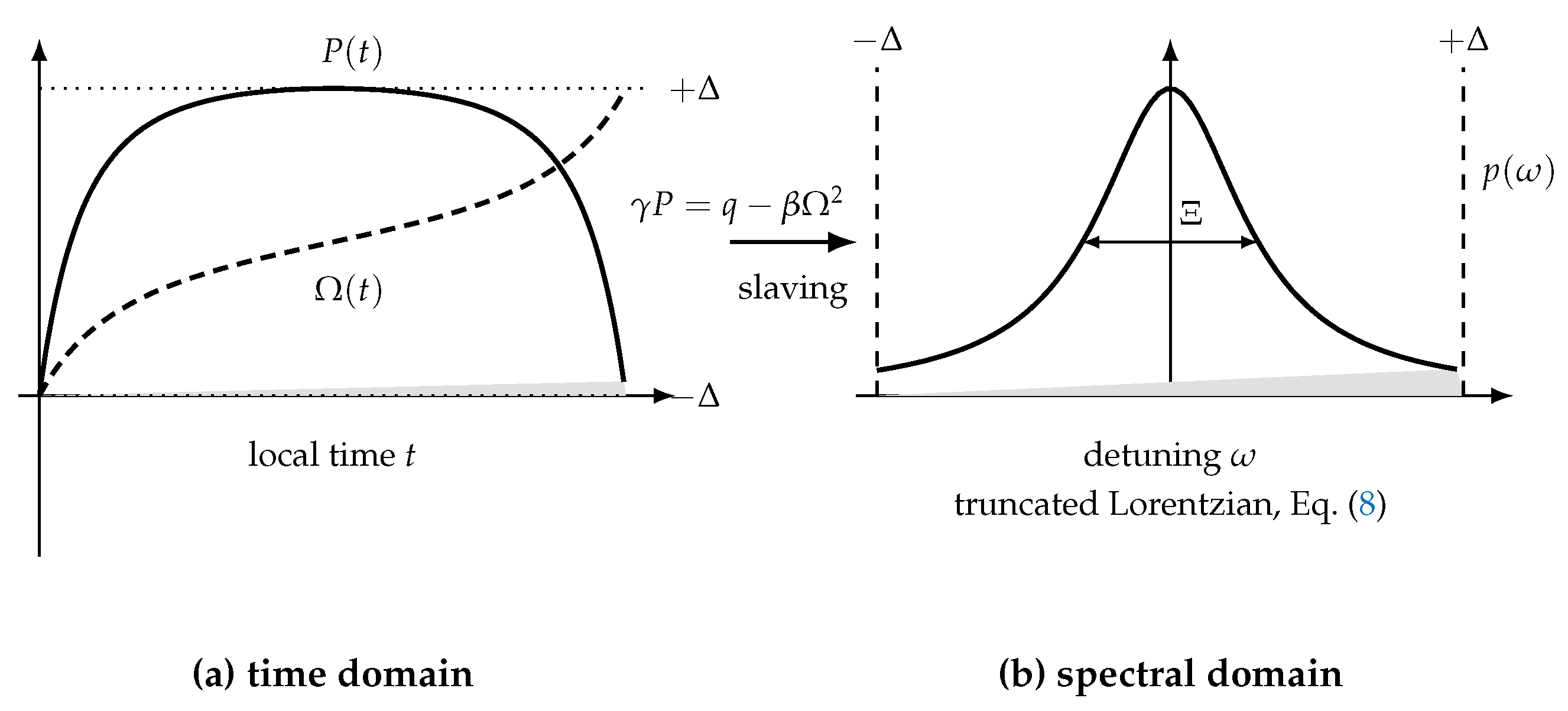
Figure 2.
The master diagram, computed from Eqs. (7), (11) and (13). Grey curves are isogains (solid: the scalable branch ; dashed: the unscalable branch ), shown for , and . The solid black curve is the vacuum-stability threshold , above which no DS exists; the dotted curve is the branch divider, on which the discriminant of (7) vanishes, and the two roots merge; the dash-dotted curve is the fidelity curve , where the two correlation scales coincide, and external compressibility is optimal. The region bounded by these three curves is the region of DSR: there , and as . Each curve is drawn only on the branch and over the interval on which it is defined. The vacuum-stability curve exists for : vanishes at , where the energy diverges (dashed horizontal asymptote), and vanishes at , where the curve terminates. The fidelity curve lies on the scalable root only for (heavy dash-dot); it meets at , , and touches the branch divider tangentially at , (dots). Below it continues on the unscalable root (light dash-dot) and no longer bounds the DSR region, whose upper boundary is taken over there by the branch divider, as (38) records; this is why the shading continues below while the heavy dash-dot does not. The value quoted in earlier statements of this construction, our own included, is the terminus of the curve and not a point of the fidelity curve, whose endpoint is , in agreement with (39).
Figure 2.
The master diagram, computed from Eqs. (7), (11) and (13). Grey curves are isogains (solid: the scalable branch ; dashed: the unscalable branch ), shown for , and . The solid black curve is the vacuum-stability threshold , above which no DS exists; the dotted curve is the branch divider, on which the discriminant of (7) vanishes, and the two roots merge; the dash-dotted curve is the fidelity curve , where the two correlation scales coincide, and external compressibility is optimal. The region bounded by these three curves is the region of DSR: there , and as . Each curve is drawn only on the branch and over the interval on which it is defined. The vacuum-stability curve exists for : vanishes at , where the energy diverges (dashed horizontal asymptote), and vanishes at , where the curve terminates. The fidelity curve lies on the scalable root only for (heavy dash-dot); it meets at , , and touches the branch divider tangentially at , (dots). Below it continues on the unscalable root (light dash-dot) and no longer bounds the DSR region, whose upper boundary is taken over there by the branch divider, as (38) records; this is why the shading continues below while the heavy dash-dot does not. The value quoted in earlier statements of this construction, our own included, is the terminus of the curve and not a point of the fidelity curve, whose endpoint is , in agreement with (39).

Figure 3.
The sign of dispersion changes the conservative equilibrium spectrum qualitatively. Curves are level sets of the linear dispersion entering the Rayleigh–Jeans distribution (15); occupancy is largest where is smallest, i.e. on the innermost level set. (a) For anomalous GDD the level sets are ellipses, and the equilibrium spectrum is an isotropic Lorentzian, shaded here by occupancy. (b) For normal GDD they are hyperbolas with the asymptotes (dashed), and coherence is skewed along space–time trajectories rather than being separately spatial or temporal. The normal/anomalous asymmetry that organizes the argument is thus already present in conservative kinetics [16].
Figure 3.
The sign of dispersion changes the conservative equilibrium spectrum qualitatively. Curves are level sets of the linear dispersion entering the Rayleigh–Jeans distribution (15); occupancy is largest where is smallest, i.e. on the innermost level set. (a) For anomalous GDD the level sets are ellipses, and the equilibrium spectrum is an isotropic Lorentzian, shaded here by occupancy. (b) For normal GDD they are hyperbolas with the asymptotes (dashed), and coherence is skewed along space–time trajectories rather than being separately spatial or temporal. The normal/anomalous asymmetry that organizes the argument is thus already present in conservative kinetics [16].

Figure 4.
Fixed external mode number versus self-generated spectral scale separation. (a) In a multimode waveguide, the eigenvalue ladder is a property of the geometry: raising the power reshuffles the occupancies towards the Rayleigh–Jeans law, but the number M of available states—and hence the “volume” variable of the equation of state (20)—is the same before and after. (b) For a strongly chirped DS the spectrum supplies its own support. The spectral edge saturates while the Lorentzian width collapses, so the two correlation scales decouple and the scale-separation index of Eq. (30) increases with the pulse energy. In the deterministic solution this is a scale-separation index and not a literal count of independent microstates; a counting interpretation would require the ensemble-coherence calibration of Section 4.3. Bars and curves are schematic.
Figure 4.
Fixed external mode number versus self-generated spectral scale separation. (a) In a multimode waveguide, the eigenvalue ladder is a property of the geometry: raising the power reshuffles the occupancies towards the Rayleigh–Jeans law, but the number M of available states—and hence the “volume” variable of the equation of state (20)—is the same before and after. (b) For a strongly chirped DS the spectrum supplies its own support. The spectral edge saturates while the Lorentzian width collapses, so the two correlation scales decouple and the scale-separation index of Eq. (30) increases with the pulse energy. In the deterministic solution this is a scale-separation index and not a literal count of independent microstates; a counting interpretation would require the ensemble-coherence calibration of Section 4.3. Bars and curves are schematic.

Figure 5.
The two correlation scales, and the two ways of obtaining them. (a) In normal GDD the spectrum is a Lorentzian of half-width truncated at , the truncation being forced by through (4): the ultraviolet cutoff is a property of the solution. (b) In anomalous GDD the same construction gives a two-horn core with algebraic wings and no truncation; the boundary of the occupied spectrum is instead supplied from outside, by the spectral filter, and defined here as an energy quantile of the windowed envelope (25) [32]. (c) Either way, the normalized time-integrated field autocorrelation is a convolution (24) of a broad envelope (dashed), whose width is the reciprocal of the spectral core, with a narrow sinc kernel (solid), whose width is the reciprocal of the cutoff. The kernel is the finest correlation interval resolved by the occupied spectrum—one “graining cell”—and the number of such cells spanned by the envelope is the scale-separation index (30), drawn here for eight graining cells. Whether that number also counts statistically independent degrees of freedom is the open question of Section 4.3. A Schrödinger soliton has no cutoff, hence no kernel distinct from its envelope, hence (Section 4.2).
Figure 5.
The two correlation scales, and the two ways of obtaining them. (a) In normal GDD the spectrum is a Lorentzian of half-width truncated at , the truncation being forced by through (4): the ultraviolet cutoff is a property of the solution. (b) In anomalous GDD the same construction gives a two-horn core with algebraic wings and no truncation; the boundary of the occupied spectrum is instead supplied from outside, by the spectral filter, and defined here as an energy quantile of the windowed envelope (25) [32]. (c) Either way, the normalized time-integrated field autocorrelation is a convolution (24) of a broad envelope (dashed), whose width is the reciprocal of the spectral core, with a narrow sinc kernel (solid), whose width is the reciprocal of the cutoff. The kernel is the finest correlation interval resolved by the occupied spectrum—one “graining cell”—and the number of such cells spanned by the envelope is the scale-separation index (30), drawn here for eight graining cells. Whether that number also counts statistically independent degrees of freedom is the open question of Section 4.3. A Schrödinger soliton has no cutoff, hence no kernel distinct from its envelope, hence (Section 4.2).

Figure 6.
Indicators of the scale-separation ratio, computed from (7), (13), (49) and (50); numerical values in Table 5. (a) Two functionals of the same ratio . The shape indicator (solid) increases monotonically and saturates at ; the shape entropy in core units, of (53) (dashed), does not saturate. The two differ by a shape-dependent term, which is why is a selected indicator rather than the entropy of the dimensionless spectrum. Both are level sets of r on the master diagram, and the fidelity curve is the particular level (dot). The full differential entropy h at fixed bin adds to and is not monotone at all: it turns over at , Eq. (56). (b) Along an isogain (, scalable branch), the internal-energy proxy (50) first grows with and then decays, while grows monotonically. The slope of (51), evaluated along that isogain, therefore passes through zero at the maximum of U—at , , just beyond the fidelity curve (solid vertical). With the slope is negative from there to resonance (light shading); with the zero is unmoved, but vanishes at , (dashed vertical), so the negative region is the finite window (61) (dark shading). Both shadings are properties of these two functionals along this continuation and are not state-function constructions. Note that it is that vanishes and that diverges, the mirror image of the textbook bounded-spectrum case.
Figure 6.
Indicators of the scale-separation ratio, computed from (7), (13), (49) and (50); numerical values in Table 5. (a) Two functionals of the same ratio . The shape indicator (solid) increases monotonically and saturates at ; the shape entropy in core units, of (53) (dashed), does not saturate. The two differ by a shape-dependent term, which is why is a selected indicator rather than the entropy of the dimensionless spectrum. Both are level sets of r on the master diagram, and the fidelity curve is the particular level (dot). The full differential entropy h at fixed bin adds to and is not monotone at all: it turns over at , Eq. (56). (b) Along an isogain (, scalable branch), the internal-energy proxy (50) first grows with and then decays, while grows monotonically. The slope of (51), evaluated along that isogain, therefore passes through zero at the maximum of U—at , , just beyond the fidelity curve (solid vertical). With the slope is negative from there to resonance (light shading); with the zero is unmoved, but vanishes at , (dashed vertical), so the negative region is the finite window (61) (dark shading). Both shadings are properties of these two functionals along this continuation and are not state-function constructions. Note that it is that vanishes and that diverges, the mirror image of the textbook bounded-spectrum case.

Figure 7.
The energy–entropy slope along the branch-pairing curves, recomputed here from (7), (13), (35), (49) and (50). Each curve is the locus on which a single pulse and a complex of identical pulses share the operating point and the total energy, i.e. . Solid , dashed 3, dotted 4, dash-dotted 5. is evaluated along each such curve and vanishes where U is stationary on it (dots), at , , and (, , , ). The dashed vertical line marks the zero obtained along the isogain continuation of Section 6.3, at . The two differ, which is the content of the path-dependence statement in the text. Ticks above the axis mark the entropy-proxy crossings of Section 6.4, which all lie at higher energy than the sign reversal. The four curves nearly coincide near their zeros, so the crossings do not form a well-separated cascade.
Figure 7.
The energy–entropy slope along the branch-pairing curves, recomputed here from (7), (13), (35), (49) and (50). Each curve is the locus on which a single pulse and a complex of identical pulses share the operating point and the total energy, i.e. . Solid , dashed 3, dotted 4, dash-dotted 5. is evaluated along each such curve and vanishes where U is stationary on it (dots), at , , and (, , , ). The dashed vertical line marks the zero obtained along the isogain continuation of Section 6.3, at . The two differ, which is the content of the path-dependence statement in the text. Ticks above the axis mark the entropy-proxy crossings of Section 6.4, which all lie at higher energy than the sign reversal. The four curves nearly coincide near their zeros, so the crossings do not form a well-separated cascade.

Figure 8.
Anomalous-dispersion indicators, computed here from the spectrum (64) under (66) with , , , , and the continuation at fixed . Solid: no hard cutoff beyond the quantile-capture rule (66). Dashed and dotted: the occupied window is capped at and 50 respectively. (a) Without the spectral cutoff, the scale-separation index rises towards the resonance. With extrinsic cutoff, saturates while keeps growing and falls. (b) The fixed-bin differential entropy rises monotonically and does not turn over, unlike its normal-dispersion counterpart (Figure 6b), because here the scale term rises with the shape term instead of competing with it. (c) The internal-energy proxy likewise rises monotonically, with no maximum. Hence throughout: the sign reversal of Section 6.3 has no anomalous-dispersion counterpart on this path.
Figure 8.
Anomalous-dispersion indicators, computed here from the spectrum (64) under (66) with , , , , and the continuation at fixed . Solid: no hard cutoff beyond the quantile-capture rule (66). Dashed and dotted: the occupied window is capped at and 50 respectively. (a) Without the spectral cutoff, the scale-separation index rises towards the resonance. With extrinsic cutoff, saturates while keeps growing and falls. (b) The fixed-bin differential entropy rises monotonically and does not turn over, unlike its normal-dispersion counterpart (Figure 6b), because here the scale term rises with the shape term instead of competing with it. (c) The internal-energy proxy likewise rises monotonically, with no maximum. Hence throughout: the sign reversal of Section 6.3 has no anomalous-dispersion counterpart on this path.

Figure 9.
Dynamical accessibility of the strongly chirped anomalous-dispersion branch under quantum-noise perturbation of (70). Color is the survival probability over shots; the black contour is the criterion, and the dashed vertical line is the chirp-control resonance (41), with . Common parameters , , , . (Left) the plane at fixed ; (Right) the plane at fixed . The values printed on the axes are those of Ref. [32] and must be multiplied by four to be read in the normalization of this paper (footnote to Section 5.2): the left panel is at here, and the right-hand axis runs over – here, against at . Reproduced from Ref. [32] (Fig. 8), published open access under CC BY.
Figure 9.
Dynamical accessibility of the strongly chirped anomalous-dispersion branch under quantum-noise perturbation of (70). Color is the survival probability over shots; the black contour is the criterion, and the dashed vertical line is the chirp-control resonance (41), with . Common parameters , , , . (Left) the plane at fixed ; (Right) the plane at fixed . The values printed on the axes are those of Ref. [32] and must be multiplied by four to be read in the normalization of this paper (footnote to Section 5.2): the left panel is at here, and the right-hand axis runs over – here, against at . Reproduced from Ref. [32] (Fig. 8), published open access under CC BY.

Figure 10.
A representative point inside the robust region: , , , and in the normalization of Ref. [32] ( here), over 64 independent noise realizations. Top: the analytical stationary-phase profile (solid) and a representative noisy final state (dashed), in power (left) and normalized spectrum (right). The table-top envelope and the two-horn core are preserved; the visible residuals sit at the pulse edges and at the central spectral dip. Bottom: distributions of the spectral-shape correlation with the analytical reference and of the final energy over the retained shots (the energy axis is in the internal units of the simulation, not in ). The upper row reproduces Fig. 9 of Ref. [32] (CC BY); the two histogram panels are author-generated data for the present manuscript, from the same ensemble.
Figure 10.
A representative point inside the robust region: , , , and in the normalization of Ref. [32] ( here), over 64 independent noise realizations. Top: the analytical stationary-phase profile (solid) and a representative noisy final state (dashed), in power (left) and normalized spectrum (right). The table-top envelope and the two-horn core are preserved; the visible residuals sit at the pulse edges and at the central spectral dip. Bottom: distributions of the spectral-shape correlation with the analytical reference and of the final energy over the retained shots (the energy axis is in the internal units of the simulation, not in ). The upper row reproduces Fig. 9 of Ref. [32] (CC BY); the two histogram panels are author-generated data for the present manuscript, from the same ensemble.

Figure 11.
Three condensations, with different entropy bookkeeping. (a) Equilibrium Bose–Einstein condensation: as the ground level of a fixed level structure acquires a macroscopic occupation and the entropy falls. (b) Rayleigh–Jeans condensation in a conservative multimode or wave-turbulent system: the inverse flux of the norm accumulates at while the direct flux of energy is removed by a sink at imposed from outside—by discretization, by a finite beam area, or by the waveguide bandwidth (Section 3.1); the mode basis is fixed and the entropy rises to its equilibrium maximum. (c) Strongly chirped DS: the spectrum is a Lorentzian of width truncated at the cutoff , which is fixed by the resonance of the DS wavenumber q with the linear branch (dotted, Equation (5)); gain enters at and the chirp carries the flux outwards to the lossy wings. Approaching DSR the spectrum passes from the fidelity condition (dashed) to the “finger” (solid) while saturates, so that the scale-separation index diverges. The shape indicator rises to , whereas the full fixed-bin differential entropy contracts, : the two conventions of Section 6.1 disagree here, and the disagreement is the content of the panel. The spectral offset vanishes in all three; only in (c) is the relevant scale generated by the state, and its identification with a statistical mode count remains conditional on the ensemble test of Section 4.3.
Figure 11.
Three condensations, with different entropy bookkeeping. (a) Equilibrium Bose–Einstein condensation: as the ground level of a fixed level structure acquires a macroscopic occupation and the entropy falls. (b) Rayleigh–Jeans condensation in a conservative multimode or wave-turbulent system: the inverse flux of the norm accumulates at while the direct flux of energy is removed by a sink at imposed from outside—by discretization, by a finite beam area, or by the waveguide bandwidth (Section 3.1); the mode basis is fixed and the entropy rises to its equilibrium maximum. (c) Strongly chirped DS: the spectrum is a Lorentzian of width truncated at the cutoff , which is fixed by the resonance of the DS wavenumber q with the linear branch (dotted, Equation (5)); gain enters at and the chirp carries the flux outwards to the lossy wings. Approaching DSR the spectrum passes from the fidelity condition (dashed) to the “finger” (solid) while saturates, so that the scale-separation index diverges. The shape indicator rises to , whereas the full fixed-bin differential entropy contracts, : the two conventions of Section 6.1 disagree here, and the disagreement is the content of the panel. The spectral offset vanishes in all three; only in (c) is the relevant scale generated by the state, and its identification with a statistical mode count remains conditional on the ensemble test of Section 4.3.
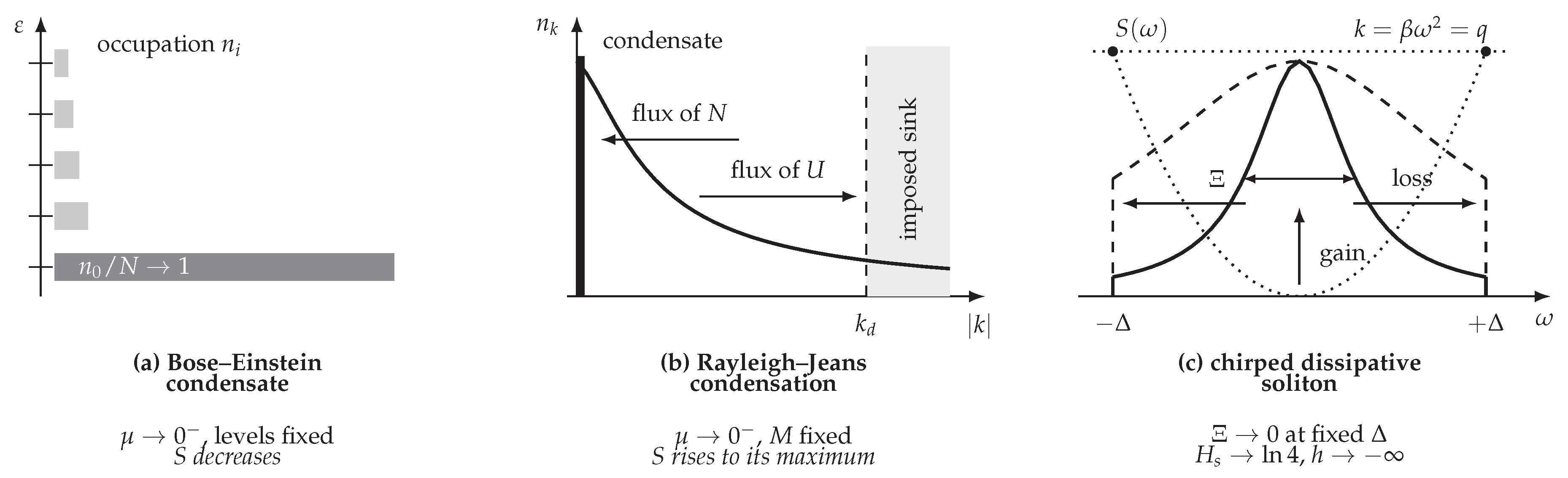
Table 1.
Status of the principal claims. E = established result of the adiabatic CQGLE analysis or of the cited literature; D = derived here under the stated assumptions; A = formal analogy, conditional on a mapping whose assumptions are listed where it is used; C = conjecture, stated with the test that would decide it. The labels recur in Section 8.
Table 1.
Status of the principal claims. E = established result of the adiabatic CQGLE analysis or of the cited literature; D = derived here under the stated assumptions; A = formal analogy, conditional on a mapping whose assumptions are listed where it is used; C = conjecture, stated with the test that would decide it. The labels recur in Section 8.
| Claim | Status | What would change the status |
|---|---|---|
| Truncated-Lorentzian spectrum, cutoff , core (Section 2.2) | E | Numerical validation outside the adiabatic window. |
| Two scales in the field autocorrelation, , (Section 4.1) | E | — (direct consequence of the spectrum). |
| Chirp alone implies partial coherence | False | Withdrawn. A deterministic chirped field is first-order coherent and has whatever its bandwidth (Section 4.3). |
| Under a specified stochastic CQGLE ensemble, is a reproducible increasing function of the deterministic scale ratio | C | Construct the ensemble, diagonalize after removing timing, phase, frequency and energy jitter, and test monotonicity and reproducibility of f. Note that f is a calibration and not an identity: r spans while , so as and the low-r branch is the single-mode limit rather than a fractional mode count. |
| as a chemical potential | A | Identify the conserved or constrained quantity to which it is conjugate; fix the energy convention (Section 6.1). |
| The cutoff is kinematic and does not require spectral filtering (Section 4.1) | E | The slaving relation (4) contains no , and chirped solutions with the same exist at [41]. |
| The Rayleigh–Jeans form of the spectrum, and every indicator built on it, requires spectral filtering (Section 4.1) | E | At the profile is convex and not thermalized [41], and the filter-free family is disjoint from the chirped branch, which requires . Would change only if a filter-free solution with a Rayleigh–Jeans spectrum were exhibited. |
| DSR as at finite (Section 5) | D | algebraic consequence of the admissibility constraints. |
| Shape indicator rises monotonically to (Section 6.1) | D | a property of one selected functional; is not the unique Shannon entropy of the dimensionless spectral shape, which depends on whether or is used to nondimensionalize. |
| diverges logarithmically at the chirp-control line, Eq. (46) | D | Coefficient verified numerically to over ; an independent derivation of the crossover would settle it. |
| changes sign at the maximum of U, (Section 6.3) | D | Numerically unchanged for the two entropy functionals tested along the isogain continuation, with both denominators verified nonzero there; independence of the continuation path is ruled out—Section 6.3 obtains on fixed-C paths, on isogains and – on branch-pairing curves, and no interior zero at all for . |
| “Negative absolute temperature” | C | Demonstrate path independence, a statistical measure and the conjugate variables; until then, negative energy–entropy slope. |
| Entropy-proxy crossing selects the multipulse state (Section 6.4) | C | Test additivity under shared gain saturation; compare with first-passage statistics in noisy simulation. |
| CQGLE ↔ driven-dissipative GPE (Section 7.1) | A | Approximate, not term-for-term: division by mixes reactive and dissipative coefficients, and a one-to-one reading requires . Reservoir elimination, noise, trapping and geometry are not mapped; the sign of requires re-derivation. |
| Chirped DS and the KPZ phase as regimes of one field theory (Section 7.6) | C | Requires the stochastic, long-wavelength reduction and a universality-class test on shot-resolved data. |
| Numerical values – for the sign reversal and – for the entropy-proxy crossing. | D | Reproducible under the branch-pairing rule and normalization adopted here. The disagreement with the values of Ref. [34] is unresolved: it has not been traced to an explicit mapping between the two definitions, and should not be attributed to normalization until it has been. |
| Along the continuation examined, anomalous dispersion shows no entropic turnover. Independently, a finite-time noisy linearized scan shows a one-sided accessibility boundary inside the algebraic existence region, not predicted by the scale-separation index; whether it is the asymptotic energy-limiting mechanism is open (Section 6.6) | D | Read from the quantum-noise stability maps of Ref. [32], which are linear, run to and use . A longer, fully nonlinear scan extended above , and a scan symmetric in , would change it. |
Table 2.
Symbols, roles and dimensions for (2). L = propagation length (or round trip), T = time, P = power. All composite quantities used later—C, , , , r—are dimensionless.
Table 2.
Symbols, roles and dimensions for (2). L = propagation length (or round trip), T = time, P = power. All composite quantities used later—C, , , , r—are dimensionless.
| Symbol | Role | Dimension | Notes |
|---|---|---|---|
| z, t | propagation, retarded time | L, T | |
| a, | field, power | , P | |
| saturated net loss | |||
| spectral filtering (inverse squared bandwidth) | |||
| group-delay dispersion | sign fixes the regime | ||
| self-phase modulation | |||
| self-amplitude modulation | |||
| SAM saturation | |||
| quintic (saturable) SPM | |||
| , | spectral support, spectral core | outputs, not parameters | |
| E | pulse energy |
Table 3.
The three traditions of Section 3, and the DS treated here. The fourth column is the one on which the argument turns: in every established framework the microstate count is a property of the apparatus, whereas for a chirped DS it is a function of state.
Table 3.
The three traditions of Section 3, and the DS treated here. The fourth column is the one on which the argument turns: in every established framework the microstate count is a property of the apparatus, whereas for a chirped DS it is a function of state.
| Framework | Dynamics; invariants | Stationary law | Microstate count and its origin | What selects the state |
|---|---|---|---|---|
| Wave-turbulence kinetics [16,17] | conservative NLS; N, | RJ, | — discretization, microscopic damping, or waveguide bandwidth; fixed | H-theorem; maximal |
| Wave condensation in a bounded system [18,19,58] | conservative; N, ; observed in a photorefractive crystal | RJ plus condensate at | from the Debye length, from the finite beam area; fixed by geometry | as above; first order once is restored |
| Mean-field NLS ensemble [62,63] | conservative, nonintegrable; , | coherent structure + Gaussian bath, | n — spectral truncation, with rescaled as ; fixed | maximum entropy ≡ minimum H at fixed N |
| Multimode optical thermodynamics [20,21,24,64] | conservative, weakly nonintegrable; , U | RJ, ; | M — guided modes below cutoff, set by core diameter, NA and wavelength; fixed | maximum number of microstates; |
| Mode locking as a phase transition [26,27] | dissipative but gradient flow; T imported as noise power | exact Gibbs measure | — cavity length over filter-limited pulse width; fixed by the cavity | exchange of free-energy minima at |
| Chirped DS (this work) | genuinely dissipative, no potential; nothing conserved, E free | truncated Lorentzian, | — generated by the pulse; a function of state, growing with E | no variational criterion; entropy and temperature crossings, checked dynamically |
Table 5.
Numerical values used in Section 6.1–6.4, recomputed for this paper from (7), (13), (35), (49) and (50) on the scalable branch. and are the maxima of the internal-energy proxy and of the fixed-bin differential entropy; , are the corresponding normalized energies. The last two columns are the denominators of (51) at , which must be nonzero for the sign reversal to be convention-independent.
Table 5.
Numerical values used in Section 6.1–6.4, recomputed for this paper from (7), (13), (35), (49) and (50) on the scalable branch. and are the maxima of the internal-energy proxy and of the fixed-bin differential entropy; , are the corresponding normalized energies. The last two columns are the denominators of (51) at , which must be nonzero for the sign reversal to be convention-independent.
| 0.01 | 1.202 | 7.03 | 1.449 | 9.06 | ||
| 0.05 | 1.208 | 7.12 | 1.455 | 9.16 | ||
| 0.10 | 1.216 | 7.24 | 1.461 | 9.29 | ||
| 0.20 | 1.234 | 7.52 | 1.475 | 9.57 | ||
| 0.40 | 1.284 | 8.28 | 1.517 | 10.32 | ||
| 1 | 1.208 | 1.45 | 4 | 16 | ||
| 0.2201 | 0.2813 | 0.3476 | 0.7519 | 1.1313 | ||
| 0.4516 | 0.5645 | 0.6596 | 0.9752 | 1.1042 | ||
Table 6.
Two-tier measurement plan. The first tier is available with existing single-shot spectroscopy; the second requires phase-sensitive field reconstruction, and only it can address the conjecture (34).
Table 6.
Two-tier measurement plan. The first tier is available with existing single-shot spectroscopy; the second requires phase-sensitive field reconstruction, and only it can address the conjecture (34).
| Target | Minimum measurement |
|---|---|
| Fixed-bin spectral entropy , Eq. (69) | Calibrated shot-resolved spectral intensity (DFT), fixed bins, stated noise-floor treatment and sensitivity. |
| Two-time kernel and , Eqs. (31), (33) | Shot-resolved complex field or directly measured first-order coherence, with removal of timing, carrier-frequency and energy jitter (a shot-dependent global phase cancels identically in J and need not be removed), with raw and conditioned kernels both reported. |
| Multipulse selection (Section 6.4) | Pulse-number statistics, branch classification, transition rates and residence times at a controlled noise level. |
| Path dependence of (Section 6.1) | Repeated continuation scans varying one specified physical control at a time (pump, filter bandwidth, GDD). |
| Anomalous-dispersion accessibility boundary (Section 6.6) | Survival statistics at controlled detuning from (41), both signs, with the exit channel classified—pulse splitting against relaxation onto the weakly chirped branch—rather than pooled. |
Table 7.
The CQGLE (2) term by term, in the convention (73). Entries marked ⇔ are identifications of terms in the equations; entries marked ↔ are correspondences of physical role only. The last column gives the momentum-space reading used in Section 3.1 and 7.2.
Table 7.
The CQGLE (2) term by term, in the convention (73). Entries marked ⇔ are identifications of terms in the equations; entries marked ↔ are correspondences of physical role only. The last column gives the momentum-space reading used in Section 3.1 and 7.2.
| CQGLE term | Symbol | Driven-open condensate, Eq. (71) | Wave-turbulence reading |
|---|---|---|---|
| Evolution coordinate | z | ⇔ time T | slow (kinetic) time |
| Transverse coordinate | t | ⇔ spatial coordinate x | conjugate to |
| Group-delay dispersion | ⇔ kinetic energy, : anomalous GDD gives , normal GDD a negative effective mass | linear dispersion , Langmuir-like | |
| Self-phase modulation | ⇔ two-body interaction, : self-focusing SPM is an attractive interaction | four-wave vertex; nonlinear frequency shift | |
| Quintic phase nonlinearity | ⇔ three-body interaction, : SPM saturation () is the repulsive term that arrests collapse of an attractive condensate | first correction to the interaction vertex | |
| Saturated net loss | ⇔ homogeneous dissipation minus pump; is the condensation threshold, i.e. the vacuum-stability border of the master diagram | uniform, k-independent sink | |
| Spectral filtering | ⇔ energy relaxation (“kinetic cooling”), damping ; Pitaevskii constant (provisional; see text) | ultraviolet sink; sets the graining scale | |
| Saturable nonlinear gain | ⇔ saturable pumping from a finite reservoir expanded to quintic order; saturation density | large-scale source; destroys N-conservation | |
| DS wavenumber | ↔ chemical potential of the condensate, Thomas–Fermi relation | soliton wavenumber in the resonance condition | |
| Lorentzian width | ↔ chemical potential of the quasiparticle gas; is condensation | RJ chemical potential, | |
| Cutoff frequency | ↔ ultraviolet cutoff regularizing , here supplied by the solution | dissipative wavenumber | |
| Correlation scales | , | ↔ healing length and condensate size | inner and outer scales; |
Table 9.
The chirped DS in the family of dissipative condensate models, ordered by what survives of the equilibrium apparatus. N is the norm (optical power or particle number), the free-energy (Lyapunov) functional. The last row is Equation (2).
Table 9.
The chirped DS in the family of dissipative condensate models, ordered by what survives of the equilibrium apparatus. N is the norm (optical power or particle number), the free-energy (Lyapunov) functional. The last row is Equation (2).
| Model | Structure | N | What selects the stationary state | |
|---|---|---|---|---|
| GPE / NLSE | Hamiltonian | conserved | conserved | conservative dynamics; a one-parameter soliton family |
| Pitaevskii-damped GPE [109,110] | decays at rate | minimization of ; source of the damping correspondence, | ||
| Metriplectic dissipative GPE [38] | Poisson bracket replaced by a metriplectic one with projector | exactly conserved | extrema of at fixed N: the case in which the equilibrium criterion survives dissipation | |
| Stochastic (projected) GPE [120] | damping and noise related by a fluctuation–dissipation relation | fluctuating | — | detailed balance; thermal equilibrium at |
| Driven-dissipative GPE ≡ CQGLE [39,40] | saturable gain, loss, energy relaxation; no potential | fixed by gain = loss | none | dynamical attractor selection; entropy and temperature crossings checked against simulation |
Disclaimer/Publisher’s Note: The statements, opinions and data contained in all publications are solely those of the individual author(s) and contributor(s) and not of MDPI and/or the editor(s). MDPI and/or the editor(s) disclaim responsibility for any injury to people or property resulting from any ideas, methods, instructions or products referred to in the content. |
© 2026 by the authors. Licensee MDPI, Basel, Switzerland. This article is an open access article distributed under the terms and conditions of the Creative Commons Attribution (CC BY) license (http://creativecommons.org/licenses/by/4.0/).
Copyright: This open access article is published under a Creative Commons CC BY 4.0 license, which permit the free download, distribution, and reuse, provided that the author and preprint are cited in any reuse.