
Submitted:
10 August 2026
Posted:
11 August 2026
You are already at the latest version
Abstract
The paper presents the design, development, and simulation of an intelligent control system for the pitch-decoupled vertical takeoff and landing (VTOL) unmanned aerial vehicle (UAV). In contrast to conventional tilt-rotor VTOL UAVs, the mechanical structure of the pitch-decoupled VTOL UAV allows passive transition from vertical to horizontal flight modes and vice versa without the use of additional servo actuators. A detailed kinematic scheme and the dynamic equations of motion of the pitch-decoupled VTOL UAV equipped with a two-degree-of-freedom robotic arm are developed using the Denavit-Hartenberg parameters and the Euler-Lagrange equations. The aerodynamic stability of the UAV is investigated, and the aerodynamic coefficients used in the complete dynamics model are derived. On this basis, a multivariable control system is developed. To address the well-known transition-phase issues of VTOL UAVs, a neural controller is designed using the reinforcement learning actor-critic method. It is shown that the proposed neural controller provides a smoother and more accurate transition phase and subsequent horizontal flight of the pitch-decoupled VTOL UAV compared with conventional and cascaded PID controllers.
Keywords:
pitch‐decoupled VTOL UAV
; control system
; transition phase
; neural controller
; robotic arm
; reinforcement learning
; actor‐critic
1. Introduction
Unmanned aerial vehicles (UAVs), including vertical takeoff and landing (VTOL) UAVs are currently widely used in both civilian and military applications. The demand for UAVs continues to grow because of their extensive range of applications in many important areas, including rescue operations, film production, package delivery, aerial photography, agriculture, reconnaissance, and military operations. Such wide-ranging applications stimulate the development of new UAV models that are more practical, versatile, easy to control, and energy-efficient.
The design and manufacturing of contemporary VTOL UAVs encounter various challenges, including control-system accuracy, energy consumption related to structural and mechanical design, and versatility of application. VTOL UAVs represent one of the most rapidly developing and scientifically significant classes of UAVs. The design of their control systems often requires fundamentally new approaches and methodologies, owing to their structural characteristics and diverse flight regimes.
Generally, there are three main types of multirotor VTOL UAVs, as well as several non-standard configurations [1,2,3]. The simplest configuration, typically used in small-sized vehicles, is a hybrid model that combines a multirotor UAV and a fixed-wing UAV (Figure 1(a)). The other two principal types of multirotor VTOL UAVs, conventionally referred to as tilt-rotor and tilt-wing VTOL UAVs, are widely used in practical applications (Figure 1(b),(c)) [4]. The main distinction between tilt-rotor and tilt-wing VTOL UAVs and the hybrid model in Figure 1(a) is the requirement for additional actuators (servomotors), which rotate either the rotors relative to the wings or the entire wings with fixed rotors relative to the UAV body. These rotations are necessary when switching between vertical takeoff and landing modes and the horizontal flight mode [5].
Irrespective of the multirotor VTOL UAV type, there are three distinct flight phases or modes:
- Multirotor mode (vertical takeoff and/or landing),
- Transition mode (switching between vertical and horizontal flight),
- Fixed-wing mode (horizontal flight).
Essentially, the control of takeoff, landing, and hovering modes can be achieved using conventional control algorithms developed for standard multirotor UAVs (quadcopters, octocopters, etc.) and fixed-wing aircraft. However, the transition mode is unique to VTOL UAVs and presents numerous challenges because of the highly nonlinear and complex nature of the vehicle dynamics during this mode. In addition, each VTOL UAV configuration shown in Figure 1 requires individual consideration because of its specific structural characteristics.
During the transition phase, strong mechanical and aerodynamic forces act on the UAV body due to variations in the thrust-vector angle. This may result in thrust loss, attitude instability, and increased complexity of the overall control problem.
In general, traditional linear controllers, such as PID, LQR, and pole-placement controllers, do not perform satisfactorily during the transition phase. Consequently, many researchers investigate various nonlinear control approaches and hybrid strategies, including gain-scheduling, sliding mode control, backstepping, and others. In some studies, the transition-control problem is often formulated as an optimal-control problem aimed at deriving optimal control laws for the transition phase. For example, in [6], the transition control of a ducted-fan VTOL UAV is formulated as a constrained Markov decision process, and constrained policy optimization is used to learn safe control policies that regulate state transitions while satisfying safety constraints. However, the solutions proposed in [6] are rather sophisticated and require significant computational resources and complex numerical algorithms [7,8].
One of the major drawbacks of the tilt-rotor and tilt-wing VTOL UAVs in Figure 1(b) and 1(c), compared with the hybrid configuration in Figure 1(a), is the necessity for additional actuators that provide transitions between takeoff/landing and horizontal flight modes.
To overcome this disadvantage, Apkarian [9,10,11] proposed a new type of tilt-rotor VTOL UAV called the pitch-decoupled UAV, which was patented in the United States [9]. The overall view of the pitch-decoupled VTOL UAV equipped with a two-degree-of-freedom robotic arm is shown in Figure 2. The main idea behind J. Apkarian’s patent is illustrated in Figure 3.
Similar to standard hybrid VTOL UAV in Figure 1(a), the fuselage of the pitch-decoupled UAV consists of two parts: the quadcopter part and the fixed-wing aircraft part (hereafter referred to as the quad and wing parts). The rotors are passively coupled to the aircraft frame about the pitch axis through a parallelogram hinge mechanism. During takeoff and landing, the propellers are positioned vertically; therefore, the UAV operates similarly to a conventional quadcopter (Figure 2 (a)). During longitudinal (horizontal) flight, the propellers rotate by degrees relative to the UAV frame and function similarly to those of a standard tilt-rotor VTOL UAV (Figure 2 (b)). A unique feature of this design is that the front and rear propellers are kinematically linked, and their rotation relative to the UAV body is achieved not by additional servomotors, as in the configuration shown in Figure 1(b), but by differential thrust generated by the front and rear rotor pairs. To improve control of the pitch axis, the UAV is additionally equipped with a fifth rotor located near the tail. The VTOL UAV also includes ailerons and an elevator to provide additional flight control during fixed-wing operation.
The main structural and kinematic features of the pitch-decoupled VTOL UAV, compared with a conventional tilt-rotor UAV, are considered in [10]. Based on a simplified mathematical model, it is shown that the vertical component of the rotor thrust depends only on the angle , which is defined as the difference between aircraft pitch angle and the relative tilt angle of the rotor hinge mechanism. The major challenges associated with controlling this type of VTOL UAV using cascaded PID controllers are discussed in the tutorial [11].
The novel pitch-decoupled VTOL UAV concept has attracted considerable attention from researchers in this field. In [12], a single PID-based controller is proposed that seamlessly manages the transition from vertical to longitudinal flight. A more sophisticated nonlinear dynamic model of the pitch-decoupled VTOL UAV, formulated as a constrained system of three rigid bodies using the Lagrangian approach, is presented in [13]. The model developed in [13] also includes an aerodynamic subsystem that generates forces and moments acting on the wing and fuselage of the aircraft. A detailed mathematical model of the pitch-decoupled VTOL UAV equipped with a robotic arm is developed in [14], and a PID-based control system for hovering mode is investigated using a Simulink model.
This paper is devoted to the development of a neural controller for a pitch-decoupled VTOL UAV equipped with a robotic arm, which provides smooth transitions between vertical takeoff and landing modes and horizontal flight mode.
The paper is organized as follows. Section 2 presents the kinematic analysis of the pitch-decoupled VTOL UAV equipped with a two-degree-of-freedom (DOF) robotic arm using the Denavit-Hartenberg formalism. In Section 3, the dynamic equations of the UAV’s angular rotations are derived using the Euler-Lagrange equations. Section 4 presents the translational dynamics of the UAV. Section 5 is devoted to the design of the attitude control system based on the developed mathematical model and conventional PID controllers. Section 6 presents the design of a matrix neural controller based on the reinforcement learning actor-critic method.
2. Kinematics of the Pitch-Decoupled UAV
In this section, a detailed kinematic scheme and the kinematic equations of the pitch -decoupled VTOL UAV equipped with a two-DOF robot manipulator are developed based on the parameters, which can be regarded as certain modifications of the well-known Denavit-Hartenberg (DH) parameters used in robotics [15]. Such an approach allows both the relative angular positions and linear displacements to be represented in a united form for an arbitrary number of reference frames (coordinate systems) using homogeneous transformation matrices [16,17]. The generalized coordinates and reference frames chosen for the derivation of kinematic equations are shown in Figure 4, where the quad part of the VTOL UAV is modeled as a flat plate with four fixed rotors.
Let denote a right-hand inertial reference frame with the origin at and the axes denoted
and , and let () denote orthogonal reference frames with origins at and axes
and
In Figure 4, is a reference frame with the origin at the center of mass (CM) of the VTOL UAV with the robotic arm. The axes of are aligned with the axes of the inertial frame . The orientation of the VTOL UAV with respect to is determined by three successive rotations of the intermediary frames , and through the yaw, roll, and pitch angles. These angles determine the first three generalized coordinates (yaw), (roll) and (pitch) of the UAV. The corresponding homogeneous transformation matrix can be written in the form:
(1)
In the matrix (1), and are zero vectors of the indicated sizes, and is the following orthogonal rotation matrix [18]:
(2)
where c and s are shorthand forms for cosine and sine, respectively. Note that the matrix (2) determines the orientation of the UAV’s body-fixed frame with respect to the inertial frame .
The next two generalized coordinates, and , describe rotations of the robotics arm with respect to the body-fixed frame . Finally, the sixth generalized coordinate, , is the pitch angle of the quad part of the UAV relative to the wing part [10]. Each of these three generalized coordinates and has an associated reference frame and a corresponding homogeneous transformation matrix . To develop the configuration kinematic equations for the pitch-decoupled UAV, we introduce the following DH-like parameters and basic transformations: , the linear displacement of the reference frame relative to along the axis ; the linear displacement of the reference frame relative to , along the axis ; the rotation (twist) of about the axis ; the rotation of about the axis . Each basic transformation has an associated homogeneous transformation matrix. The product of these matrices yields the resulting homogeneous transformation matrix
(3)
I = 4, 5, 6.
The introduced parameters , and the matrix (3) differ from the standard DH parameters [15] but are more convenient for describing the kinematics of the UAV in Figure 4. Based on the kinematic model shown in Figure 4, we have
, (4)
(5)
Besides the presented reference frames , an additional frame is introduced. This frame is not associated with any generalized coordinate but is required to describe the position and orientation of the tail rotor and of the quad part of the UAV. The corresponding homogeneous transformation matrix has a simple form
(6)
By multiplying the introduced matrices in accordance with the kinematic model in Figure 4, we obtain the position and orientation of each reference frame relative to the initial reference frame . Performing the multiplications yields the following homogeneous transformation matrices:
(7)
To calculate the torques generated by the rotors, it is necessary to determine the rotor displacements with respect to the CM of the UAV. Note that the positions
of the four rotors on the quad part in the reference frame are determined as follows:
(8)
where is the distance from the rotors to the origin and the fourth, a unity, coordinate is added to conform with the homogeneous matrix notations.
Similarly, the displacement vector of the fifth (tail) rotor in the reference frame can be defined as
Multiplication of the rotor displacement vectors by the corresponding transformation matrices yields
(10)
the first three coordinates of which determine the rotor displacements (rotors positions vectors) in the reference frame }, which is attached to the CM of the system. In what follows, we denote the indicated three-dimensional vectors by . Furthermore, let us denote a three-dimensional vector composed of the first three entries of the second column of the matrix , and , a vector formed in the same manner from the third column of :
(11)
Note that the vector determines the direction of the thrusts
, generated by the first four rotors, in the frame , and determines the direction of the thrust in the frame .
Then, the total torque generated by the five rotors can be expressed as
(12)
In the equation (12),
(13)
(14)
where is the symbol of cross product, are the torques acting on the UAV and generated by all five rotors, is a constructive parameter determining the reaction torques acting on the airframe by the rotors of the quad part, and is the same parameter of the tail (fifth) rotor [3].
Note that in the vertical takeoff and landing flight modes, the generalized coordinate (the passive pitch angle of the quad part) is equal to zero and the total vertical thrust of the quad part rotors is
(15)
This thrust is directed along the body-fixed axis . In the horizontal flight mode, the passive pitch angle is equal to , and the total thrust (15) is directed along the axis .
It should also be noted that, besides the rotor thrusts, the generalized coordinates
, which determine the orientation of the UAV, are affected by tilts of the elevator and the ailerons. This point is discussed further in the derivation of the dynamics equations of the pitch-decoupled UAV.
The block diagram shown in Figure 5 illustrates schematically the kinematic links of the pitch-decoupled UAV.
Here, the arrows directed from left to right represent the torques or forces generated by the rotors, actuators of the robotic arm (), the ailerons (), and the elevator plus the fifth (tail) rotor and are the torques generated on the quad frame about the roll and yaw axes, respectively, and is the rotation matrix
(16)
3. Rotational Dynamics of the Pitch-Decoupled UAV
The dynamics equations of angular rotations of the pitch-decoupled VTOL UAV are derived using the Euler-Lagrange equations, which for a mechanical system with six degrees of freedom have the following form [19,20]:
(17)
where
(18)
is the Lagrangian, defined as the difference between the total kinetic and potential energies; are the generalized coordinates, and are generalized forces arising from all external and dissipative forces and torques, including those arising from potential energy and from the elevator and ailerons deflections [21].
Let denote the vector of angular velocity of the UAV’s wing part (of the fuselage), to which the body-fixed frame is attached. Then the kinetic energy of the wing part (or, in other words, of the UAV’s fuselage) is equal to
(19)
where
(20)
is the inertia tensor of the fuselage.
The vector in (19) can be parameterized by generalized coordinates , , and (by yaw, roll, and pitch angles) as [22]
(21)
where , and
(22)
Then, the kinetic energy (19) can be rewritten in the form
(23)
Note that the generalized coordinates
, and in the kinematic model shown in Figure 4 are associated with three rigid bodies. Each of these bodies (two links of the robotic arm and the quad part) has one degree of freedom relative to the bodies, to which they are attached. This allows the kinetic energies , and of these bodies to be represented in a unified form, using the homogeneous transformation matrices, as
(24)
(25)
(26)
where
(27)
are the pseudo inertia matrices, and are first inertia moments with respect to the corresponding rotation axis [20,21].
It should be noted that the transformation matrix in (26) does not depend on the generalized coordinates and .
To make the following expressions more compact, let us introduce special notations for the traces of transformation matrices:
(28)
(29)
(30)
Then the total kinetic energy of the UAV’s rotational motion can be represented in the form
(31)
The potential energy of the pitch-decoupled UAV is given by the equation
(32)
where is the gravitational vector, are the masses of the fuselage and the corresponding rigid bodies, are the positions of the CM of the th body in the associated coordinate frame [21].
Substitution of the equations (31) and (32) into (17) yields the dynamics equations of the pitch-decoupled UAV. For the vector of the Euler angles
and we have:
(33)
where
, (34)
denotes the partial derivative with respect to ; is the vector of torques (12); and are the torques produced by the ailerons and elevator tilts; is an internal torque, generated by the first actuator of the robotic arm; is a three-dimensional vector with the components
(35)
Equation (33) can be written in a more compact and transparent form [22]. Note that the time derivative of the angular velocity vector in (21) is
(36)
Then the equation (33) can be written as
(37)
where , and denote the moments generated by ailerons and elevator tilts, the superscript denotes the combination of matrix transposition and inversion, and the transposed inverse of is
(38)
Comparing this expression with the Newton-Euler’s equations of rotational motion of a rigid body in the body-fixed frame [22]
(39)
implies
(40)
and the equation (37) can be written in the following compact form:
(41)
This equation, in which the last term on the left-hand side describes dynamic cross-coupling of the fuselage and the robotic arm, is more convenient for analysis and design of the attitude control system in the takeoff and landing modes.
The dynamics equations for the generalized coordinates
and are
(42)
(43)
where is internal torque produced by the second actuator of the robotic arm, and
(44)
Equations (33), (42)-(44) can be written in the matrix form
(45)
The entries of the symmetric inertia matrix in (45) are
Mij = (STI0S)ij+ aij(4) + aij(5) + aij(6), i,j ≤ 3,
The entries of the Coriolis/centrifugal terms (Christoffel symbols) of the matrix in (45) are determined in terms of the coefficients (46) as
(47)
The components of the gravity vector in (45) are
(48)
Finally, the components of the vector in (45) are
(49)
(50)
The derived differential equations of the rotational motion (33)-(50) were used in the development of the comprehensive (expanded) dynamic model of the pitch-decoupled UAV in the Simulink package environment.
4. Translational Dynamics of the UAV
The main forces acting on the pitch-decoupled UAV during the horizontal (longitudinal) flight are schematically shown in Figure 5, where are the thrusts generated be the five rotors, is the total thrust of the quad part’s four rotors, and are aerodynamic forces.
If all forces are represented with respect to the inertial reference frame, then, according to Newton’s second law, the simplified differential equations describing the translational motion of the UAV are given by the equation
(51)
where vector represents the linear position of the UAV in the inertial reference frame, is the total mass of the UAV, is the total thrust of the quad part rotors (15), is the orthogonal rotation matrix (2), is the gravitational constant,
denotes the aerodynamic forces acting on the UAV in the wind frame. For simplicity, sideslip forces are neglected, and the aerodynamic forces are assumed to be transformed to the inertial reference frame.
To calculate the aerodynamic characteristics of the pitch-decoupled UAV, it is necessary to determine its lift force , drag force , and the aerodynamic pitching moment about the pitch axis, which are given by the following expressions [23,24]:
where is an angle of attack, and the lift drag and pitching moment coefficients are equal to
In the expressions (52), is the air density, is the wing area, is the flight velocity relative to the air, c is the mean aerodynamic chord [25]. Besides, the coefficients
, and in (53) are actual aerodynamic lift and drag forces, and the pitching moment.
The study of the UAV’s aerodynamic characteristics, including the lift and drag coefficients, as well as the stability properties, was performed using the “XFLR5” aerodynamics simulator [26,27,28], considering external forces applied along the longitudinal and lateral axes of the UAV. Figure 6 illustrates the lift, drag and pitching-moment coefficients obtained for different aerodynamic airflow simulation runs. Figure 7 presents the results of analyzing the aerodynamic stability under external forces. The graphs in Figure 7 indicate that the UAV is aerodynamically stable in both longitudinal and lateral directions. The results of aerodynamic simulations were used in the design of the neural controller described in Section 6.
5. Control System of the Pitch-Decoupled UAV
In this Section, the control of the pitched-decoupled UAV in different flight modes is considered in detail. Unlike the transient modes common to tilt-rotors UAVs, in which the UAV switches between the vertical and horizontal flights by tilting the rotors from to or vice versa, special attention in Subsection 5.2 is devoted to a flight regime, in which the pitch angle of the quad part is constant but not equal to the limiting (marginal) values or . Geometrically, this corresponds to a “sloped” (climb or descent) flight of the pitch-decoupled UAV. Schematically, the sloped flight mode is illustrated in Figure 8. In this mode, the pitch angle of the plane is zero, and the given constant (but not or ) tilt of the quad part is maintained by a special feedback loop, the error signal of which is calculated as a difference of the given tilt and the signal of the potentiometer measuring the relative tilt of the quad part.
For any given “intermediate” tilt of the quad part, there are three different situations. If the vertical component of the total thrust is equal to the gravitational constant (Figure 8a), the UAV is in the horizontal flight with tilted rotors. If the vertical component is larger (), the UAV is in the climb flight (Figure 8b). Finally, if the UAV is in the descent flight. Note that in all these situations, the zero pitch angle of the UAV is provided by the control system of the tail rotor.
5.1. Control System in Takeoff, Landing, and Hovering Modes
We specifically discuss the flight of the pitch-decoupled UAV in the standard takeoff, landing, and hover modes because in these modes the pitch-decoupled UAV is controlled like a conventional quadcopter. Moreover, the robotic arm is usually used when the UAV is in hover mode. In the present configuration, in these modes, the quad pitch angle (also referred to as angle) is zero and the quad part is rigidly fixed to the UAV’s fuselage.
To proceed, we shall make some assumptions and simplifications needed for the design of the corresponding controllers in the mentioned modes. First, we assume that the mass and inertia matrix of the quad part are accounted for in the mass and in the inertia matrix of the fuselage, where the matrix is assumed to be diagonal. This simplifies the differential equations (32), (42), (43), in which all the terms containing index 6 must be eliminated. In addition, the equation (44) must be discarded.
Generally, in controlling the flight of quadcopters, the altitude and rotation angles (roll , pitch , and yaw ) are usually chosen as four control variables [29].
Below, we shall assume that the angles and angular velocities of the UAV are so small that nonlinear terms in the dynamic equations of rotational motions can be neglected, the cosines of all angles are approximately equal to one, and sines of the angles are zero. At this stage, we assume that there are no dynamic cross-couplings between the fuselage of the UAV and the robotic arm.
On these assumptions, the dynamics equations of multirotor UAVs have the following linearized form [3,29]:
, (54)
, , (55)
where is the mass of the UAV; g – the gravitational constant; is the diagonal tensor of inertia with the components on the principal diagonal; vector
combines the principal non-conservative forces and moments applied to the UAV airframe by the aerodynamics of the four quad part rotors (assuming no external disturbances); and are inertia moments of the robotic arm links.
Denoting by the four-dimensional vector of thrusts (), the mapping of to the vector can be written in matrix form
(56)
In (56), the full-rank numerical matrix for the quad part rotors allocation in Figure 4 is equal to
(57)
where is the distance of the rotors from the point in Figure 4. Structurally, the matrix (59) describes the kinematic cross-coupling between the separate channels of the UAVs in hover mode.
The matrix block diagram of the UAV’s control system in hover mode and of the two-dimensional control system of the robotic arm is shown in Figure 9.
In Figure 9: is an identity matrix; is an identity matrix is a two-dimensional vector with components and ; is a projection matrix
; (58)
is the transfer function of brushless DC motors (rotors) of the quad part; is a diagonal matrix of the transfer functions ;
(59)
is the transfer matrix of the matrix regulator with the numerical matrix equal to
(60)
The superscripts in Figure 9 denote the reference (input) signals.
The transfer function in Figure 9 represents the identical transfer functions of separate channels of the robotic arm and has the form
(61)
where is the transfer function of the link actuators (DC motors), and is the transfer function of the controllers.
Assuming for simplicity that the transfer functions () in (59) are identical, that is , the transfer matrix of the open-loop UAV’s control system in hover mode takes the form
(62)
where the matrix has the following block-diagonal form:
(63)
The dynamics of the DC motors in (61) and (62) are approximated by the first-order transfer functions
, (64)
Note that if the matrix in the regulator (59) is chosen as in (60), then the transfer matrix of the open-loop system reduces to the diagonal form
(65)
This equation implies that the attitude control channels of the UAV in hover mode are decoupled (since matrix is assumed diagonal) and the design of controllers in these channels can be performed as for common single-input single-output (SISO) control systems [30]. The PD controllers with the following transfer function:
(66)
were used as controllers in (65). This transfer function was obtained by applying the graphical user interface (GUI) pidTuner in MATLAB [30]. Analogously, the PD controllers of the form:
(67)
were used as the controllers of the robotic arm.
The step responses of the attitude control system of the pitched-decoupled UAV with the robotic arm in hover mode are shown in Figure 10. The control of the UAV altitude is considered in the next section.
5.2. PID Control of the Pitch-Decoupled UAV in Transition and Sloped Modes
In this section, we concentrate mainly on the dynamics of the pitched-decoupled UAV in transition mode using standard PID controllers. A control architecture is proposed, in which, to improve the controllability of the UAV, additional velocity-control loops for the three translational axes are introduced. In this system, the control of the UAV in the transition mode essentially reduces to the velocity control of the UAV’s fuselage. The selection of parameters of PID controllers was performed by automatic design tools available in Control System Toolbox in MATLAB [30]. Dynamics analysis of the control system was performed in the Simulink environment, based on the developed nonlinear mathematical model of the UAV, in which, also, the aerodynamic forces (lift and drag) were accounted for. The matrix block diagram of control system of the pitched-decoupled UAV in the transition mode is shown in Figure 11. It should be noted that, virtually, the robotic arm is not (or, practically, cannot be) used in the transition mode. For that reason, the control system of the robotic arm is not shown in the block diagram in Figure 11. Moreover, the aerodynamic (lift and drag) forces, the influence of which is of a complex nonlinear nature, are also not presented in the block diagram. In Figure 11: and are the inputs and outputs of the velocity control system; is the diagonal matrix of the following PID controllers:
, , ; (68)
is the matrix of the form
; (69)
and
(70)
is the PID controller of the passive pitch angle ; is the inertia moment of the quad part about the rotation axis.
Let us consider the transition phase of the pitch-decoupled UAV with the PD controllers (70) for two scenarios. Figure 12 shows the results of 3D simulation in case when the UAV switches from hover mode to longitudinal flight by tilting the quad part by . The dynamic model of the UAV was developed based on nonlinear equations ()-() and the results of aerodynamic simulation of the UAV presented in Section 4. In this scenario, the UAV starts the flight at and gains the prescribed altitude of 85 m. At , the UAV switches to longitudinal flight. As can be seen from Figure 12, during the transition phase, the UAV’s altitude drops to 16 m (at ). Afterwards, due to aerodynamic characteristics of the UAV, it starts gaining velocity and altitude. The graphs in Figure 13 show the and altitude response graphs.
In the second scenario, the UAV is in hover mode at the prescribed altitude 5 m, and at 8 s, the passive pitch angle changes from to . Figure 14 shows the changes in the angle and the flight altitude. Figure 15 presents the horizontal velocity, as well as the aerodynamic lift and drag forces of the UAV. Figure 16 shows the total thrust generated by the rotors, which decreases after completing the transition phase due to the increase in the aerodynamic lift force.
The parameters of the PID controllers (68) in the velocity control system are determined based on the linearized model of the UAV and for the fixed value of the angle . In practical flights, the required angle is calculated in advance and introduced manually by the operator. The required parameters of the velocity PID controllers may change substantially for different angles . The most common strategies to overcome that difficulty are based on using adaptive, gain-scheduling, and intelligent control techniques, or their combinations [31,32,33,34], as well as other strategies [29,30].
6. Actor-Critic Method and Neural Controller
One of the most effective approaches for designing intelligent controllers is reinforcement learning because it allows one to develop an optimal control policy through interaction with the environment, particularly for systems that are highly nonlinear, uncertain, or difficult to model accurately [35,36,37]. Among reinforcement learning algorithms, the actor-critic family has become one of the most widely used in robotics, UAVs, autonomous vehicles, and process control because it combines the strengths of policy-based and value-based methods [38,39,40].
This section describes a neural controller designed and trained using the reinforcement-learning actor–critic method. The objective is to develop a controller capable of ensuring a smooth transition of a pitch-decoupled UAV from quadcopter mode to airplane mode and back in various working conditions, while minimizing tracking errors.
Briefly, the training procedure can be described as follows. At each time step , the main control agent selects an action, receives a reward from the environment, and transitions from state to state The ultimate objective of reinforcement learning is to maximize the expected discounted return over time
(71)
where is the discount factor.
If an agent follows policy at time , then denotes the probability of selecting action while the system is in state . Maximizing the expected return yields the optimal policy for the agent.
The action-value function associated with policy is denoted by and is given by the following expression:
The central concept of reinforcement learning is represented by the Bellman equation,
This equation defines the optimal action-value function that the agent must learn iteratively. In this study, the Deep Deterministic Policy Gradient (DDPG) algorithm was employed [41,42]. DDPG uses an actor–critic architecture in which the critic serves as a value-function approximator, while the actor is trained using feedback from the critic by selecting actions that maximize the estimated critic value. The actor–critic structure used for the pitch-decoupled UAV training is illustrated in Figure 17.
The actor network is denoted by and parameterized by , whereas the critic network is parameterized by , and its loss function has the following form:
where is the output of the critic network, and the target value is defined as:
The overall policy gradient is given by the following expression:
Here, and are the gradients of the critic and actor neural networks, respectively. Consequently, the actor is trained based on the action values returned by the critic network. It is important to note that the target value employs the same actor-critic networks with the same parameters which may cause instability during training. To address this issue, target copies of the actor and critic networks, and , are introduced. Their parameters and are updated more slowly than those of the primary networks using a soft update factor :
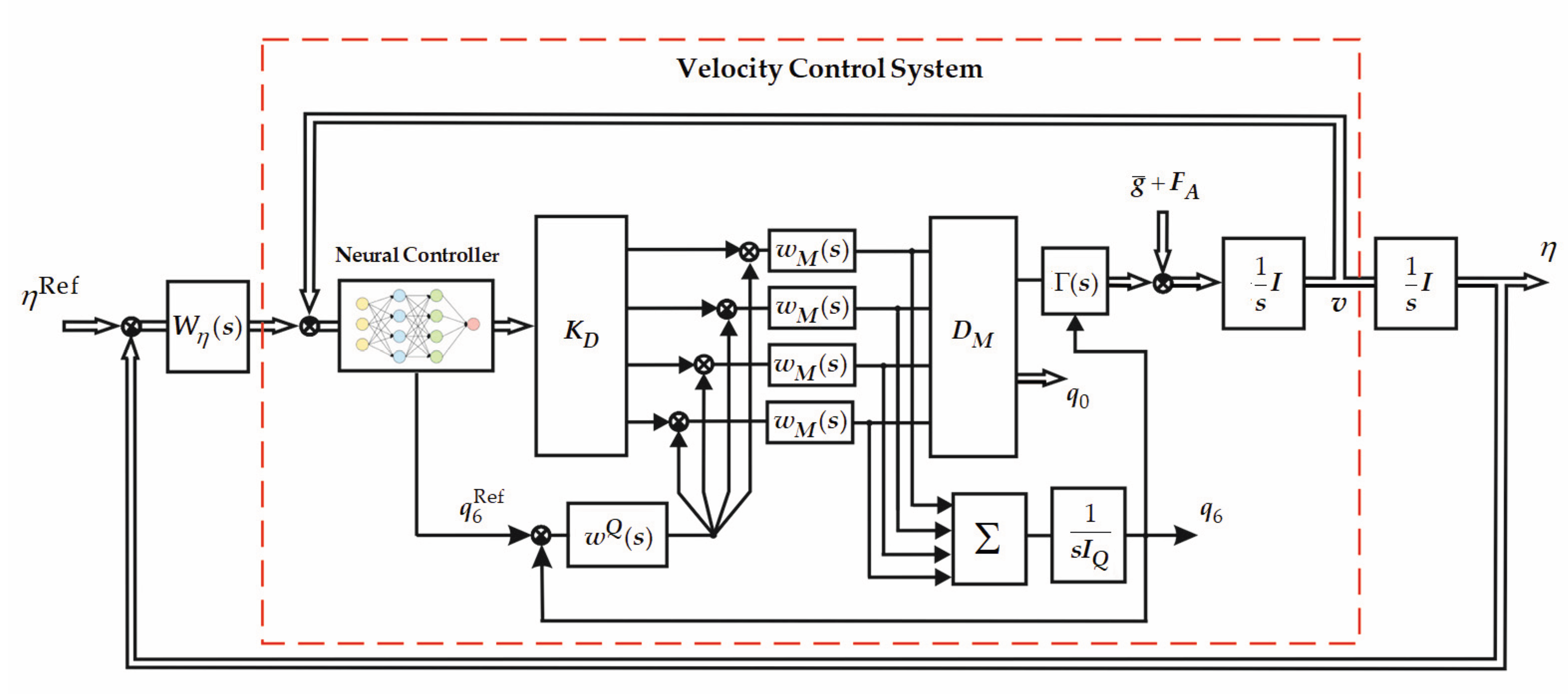
As described previously, the neural controller replaces the conventional velocity PID controllers to achieve smooth transition behavior and accurate velocity tracking. The resulting velocity control system architecture, incorporating the neural controller, is shown in Figure 18. Here, the neural controller continuously governs the passive pitch angle depending on the current state of the control system, required flight regime and flying conditions.
The state vector is defined as follows:
where
are the velocity tracking errors.
The reward function is defined as follows:
where are the weighting coefficients of the reward components, and the term represents the actuator effort penalty. The training episode is terminated if any of the following conditions is violated:
The pitch-decoupled UAV model and the training procedure were implemented in the Simulink environment using the Reinforcement Learning Designer Toolbox for agent construction [43]. Figure 19 presents the overall training process, during which the agent progressively improves its control policy by maximizing the expected return over successive episodes.
To evaluate the behavior of the control system incorporating the neural controller, two transition-phase scenarios were investigated. In each scenario, the pitch-decoupled UAV takes off and reaches a specified altitude . Then, at , the transition phase is initiated during which the UAV accelerates toward a prescribed horizontal velocity Both scenarios were simulated in the Simulink environment using different values of the reference parameters , and , :
Scenario 1:
Scenario 2:
Figure 20 and Figure 21 present the simulation results for Scenario 1, and Figure 22 and Figure 23 for Scenario 2, where denotes the passive pitch angle and is the altitude. In both cases, the transition phase proceeds smoothly, without overshoot or steady-state error, confirming the effectiveness of the proposed neural controller.
Figure 21 and Figure 23 show the horizontal and vertical velocity responses (blue lines) of the pitch-decoupled UAV together with their reference signals (black dot lines) for Scenarios 1 and 2, respectively. The results demonstrate that the neural controller ensures smooth transition and stable flight at the prescribed horizontal velocities while maintaining minimal tracking error. The transition phase begins when the reference horizontal velocity changes from zero to the prescribed constant value. The primary function of the neural controller is not to directly initiate the transition, but rather to track the reference velocities with minimal error by adjusting the angle and rotors’ total thrust.
The required () angle, which is calculated by the neural controller, is shown in Figure 20 and Figure 22. In Scenario 2, the transition phase begins before the pitch-decoupled UAV reaches its reference altitude. Nevertheless, the neural controller successfully manages the transition without producing overshoot or steady-state errors.
The simplified, without the altitude and attitude control subsystems, block diagram of the pitch-decoupled UAV’s control system with the velocity neural controller is shown in Figure 24.
Here, is a diagonal position controller with, usually, standard SISO PID controllers on the main diagonal. In the block diagram, there are two multivariable feedback loops, and one passively controlled (by difference of the paired thrusts) SISO loop, which governs the transitions between different flight modes during entire flight envelope. The altitude and attitude control subsystems, which operate during the hover and standard vertical takeoff and landing modes, as well as control system of the robotic arm, are discussed in Subsection 5.1.
7. Discussion
The article addresses an important challenge in pitch-decoupled VTOL UAV operation: achieving reliable and smooth transitions between hovering and fixed-wing (horizontal-flight) modes. Its principal contribution is the application of an actor–critic reinforcement-learning velocity controller to a pitch-decoupled UAV architecture that differs substantially from conventional tilt-rotor systems. In addition, the study considers a pitch-decoupled UAV equipped with a two-DOF robotic arm and derives a complete mathematical model of the system using modified Denavit–Hartenberg parameters. The proposed approach can accommodate UAVs equipped with robotic manipulators of various configurations and with an arbitrary number of degrees of freedom.
The present study focuses on investigating the main characteristics of the pitch-decoupled UAV control architecture and on designing a neural controller. Therefore, control of the pitch-decoupled UAV in conventional fixed-wing flight—for example, through the elevator, ailerons, or their combination—is not considered. In addition, the SISO tail-rotor control system is assumed to operate perfectly; that is, it is assumed to maintain the fuselage pitch angle at zero during flight. A comprehensive investigation of the pitch-decoupled UAV’s dynamics that accounts for these factors is beyond the scope of this paper.
Another distinctive feature of the study is that the UAV control architecture is formulated within the multivariable control-system framework. This formulation enables clear representation of the kinematic and dynamic cross-couplings among the subsystems and blocks that constitute the overall control system.
Compared with closely related studies on pitch-decoupled UAV control [10,11,12,13], the principal distinguishing features of the present work are the proposed DDPG-based transition controller and the inclusion of a two-DOF robotic arm in the multibody model.
Nevertheless, the proposed neural controller has several limitations, some of which are inherent to reinforcement-learning-based control. At this stage, robustness, stability, and safety have not been evaluated under variations in mass, robotic-arm configuration and payload, aerodynamic coefficients, wind disturbances, sensor noise, or partial actuator failures. These limitations, together with the need for experimental validation and practical deployment of the neural controller, define important directions for future research.
A further promising direction is the development of a hybrid control architecture for the pitch-decoupled UAV that integrates a learning-based controller with a classical model-based controller. Such architectures may provide an effective means of improving stability, robustness, and practical reliability of the UAV’s control system [33,34].
8. Conclusions
This study develops a modeling and control framework for a pitch-decoupled VTOL UAV with a two-DOF robotic arm. The platform’s passive coupling mechanism offers an attractive alternative to conventional tilt-rotor systems by using differential thrust rather than dedicated rotor-tilting actuators. The article combines kinematic and dynamic modeling, aerodynamic analysis, conventional PID-based control, and a DDPG actor–critic neural controller for transition flight. The simulation results demonstrate that the proposed neural controller provides better performance and tracking accuracy during transition modes than the conventional PID controller by continuously governing the passive pitch angle of the pitch-decoupled VTOL UAV.
Author Contributions
Conceptualization, J.A., N.N., O.G. and H.D.; methodology, J.A., N.N., O.G., Z.K. and H.D.; software, N.N., O.G., A.K., G.K. and K.B.; validation, K.B., V.M., G.K. and Z.K.; formal analysis, K.B., V.M., G.K. H.D. and A.K.; investigation, J.A., N.N., O.G.; data curation, K.B., V.M., Z.K. and G.K..; writing—original draft preparation N.N., O.G and A.K.; writing—review and editing, O.G., N.N and J.A.; visualization, K.B., V.M., G.K. and A.K.; supervision, O.G. and N.N..; project administration, O.G. and N.N. All authors have read and agreed to the published version of the manuscript.
Funding
This research received no external funding.
Data Availability Statement
The original contributions presented in this study are included in the article. Further inquiries can be directed to the corresponding author.
Conflicts of Interest
The authors declare no conflicts of interest.
Abbreviations
The following abbreviations are used in this manuscript:
| VTOL | Vertical Takeoff and Landing |
| UAV | Unmanned Aerial Vehicle |
| CM | Center of Mass |
| PID | Proportional-Integral-Derivative |
References
- Hassanalian, M.; Abdelkefi, A. Classifications, applications, and design challenges of drones: A review. Prog. Aerosp. Sci. 2017, 91. [Google Scholar] [CrossRef]
- Huang, Y.; Thomson, S.; Hoffmann, C.; Lan, Y.; Fritz, B. Development and prospect of unmanned aerial vehicle technologies for agricultural production management. Int. J. Agric. Biol. Eng. 2013, 6, 1–10. [Google Scholar] [CrossRef]
- Mahony, R.; Kumar, V.; Corke, P. Multirotor Aerial Vehicles: Modeling, Estimation, and Control of Quadrotor. IEEE Robot. Autom. Mag. 2012, 19, 20–32. [Google Scholar] [CrossRef]
- Saeed, A.S.; Younes, A.B.; Islam, S.; Dias, J.; Seneviratne, L.; Cai, G. A review on the platform design, dynamic modeling and control of hybrid UAVs. Proc. 2015 Int. Conf. Unmanned Aircr. Syst. (ICUAS) 2015, 2015, 806–815. [Google Scholar] [CrossRef]
- Flores, G.; Lozano, R. Transition flight control of the quad-tilting rotor convertible MAV. Proc. 2013 Int. Conf. Unmanned Aircr. Syst. (ICUAS) 2013, 2013, 789–794. [Google Scholar] [CrossRef]
- Fu, Y.; Zhao, W.; Liu, L. Safe Reinforcement Learning for Transition Control of Ducted-Fan UAVs. Drones 2023, 7, 332. [Google Scholar] [CrossRef]
- Escareño, J.; Stone, R.H.; Sanchez, A.; Lozano, R. Modeling and control strategy for the transition of a convertible tail-sitter UAV. Proc. 2007 Eur. Control Conf. (ECC) 2007, 2007, 3385–3390. [Google Scholar] [CrossRef]
- Escareño, J.; Salazar, S.; Lozano, R. Modelling and Control of a Convertible VTOL Aircraft. In Proceedings of the 45th IEEE Conference on Decision and Control, 2006; pp. 69–74. [Google Scholar]
- Apkarian, J. Hybrid Multicopter and Fixed Wing Aerial Vehicle. 2018. Available online: https://image-ppubs.uspto.gov/dirsearch-public/print/downloadPdf/9873508.
- Apkarian, J. Pitch-decoupled VTOL/FW aircraft: First flights. Proceedings of the 2017 Workshop on Research, Education and Development of Unmanned Aerial Systems (RED-UAS) 2017, 2017, 258–263. [Google Scholar] [CrossRef]
- Apkarian, J. Attitude Control of Pitch-Decoupled VTOL Fixed Wing Tiltrotor. 2018. [Google Scholar] [CrossRef]
- Patience, C. A.; Nahon, M. Control of a Passively-Coupled Hybrid Aircraft. 2020 International Conference on Unmanned Aircraft Systems (ICUAS), Athens, Greece, 2020; pp. 1620–1627. [Google Scholar] [CrossRef]
- Chiappinelli, R.; Cohen, M.; Doff-Sotta, M.; Nahon, M.; Forbes, J. R.; Apkarian, J. Modeling and Control of a Passively-Coupled Tilt-Rotor Vertical Takeoff and Landing Aircraft. 2019 International Conference on Robotics and Automation (ICRA), Montreal, QC, Canada, 2019; pp. 4141–4147. [Google Scholar] [CrossRef]
- Singh, K. WORKING OF ROBOTIC ARM IN INDUSTRIES. 2021, 38. [Google Scholar] [PubMed]
- Craig, J.J. Introduction to Robotics: Mechanics and Control; Prentice Hall, 2005; 408 pp. [Google Scholar]
- Niku, S.B. Introduction to Robotics: Analysis, Control, Applications; Whilley, 2019. [Google Scholar]
- Mason, M.T. Mechanics of Robotic Manipulation; The MIT Press, 2001. [Google Scholar]
- Henderson, D.M. Euler angles, quaternions, and transformation matrices for space shuttle analysis // Nasa Shuttle Program, Mission Planning and AnalysisDivision; July 1977; p. 11. [Google Scholar]
- Siciliano, B.; Khatib, O. (Eds.) Springer Handbook of Robotics; Springer, 2008; p. 1611 pp. [Google Scholar]
- Paul, R.P. Robot Manipulators: Mathematics, Programming and Control; The MIT Press, 1981; p. 279 pp. [Google Scholar]
- Jazar, R.N. Theory of Applied Robotics: Kinematics, Dynamics, and Control; Springer, 2010; p. 905 pp. [Google Scholar]
- Bernstein, D.S.; Goel, A.; Kouba, O. Deriving Euler’s Equation for Rigid-Body Rotation via Lagrangian Dynamics with Generalized Coordinates. Mathematics 2023, 11, 2727. [Google Scholar] [CrossRef]
- Durham, W. Aircraft Flight Dynamics and Control; Wiley, August 2013; p. 306. [Google Scholar]
- Cory, R.; Russ, T. Experiments in Fixed-Wing UAV Perching. AIAA Guidance, Navigation and Control Conference and Exhibit AIAA Guidance, 2008; p. 12. [Google Scholar]
- Anderson, J.D. Fundamentals of Aerodynamics, 6th ed.; McGraw-Hill Education: New York, NY, USA, 2017; ISBN 978-1259129919. [Google Scholar]
- Sanchez, F. Aerodynamics: Airfoil Analysis Using XFLR5 // Universidad Carlos III de Madrid 2017. 11. [PubMed]
- Sharma, S. Analysis of a Tiltrotor Vertical Take-off and Landing Unmanned Aerial Vehicle: CFD Approach. IOP Conf. Ser.: Mater. Sci. Eng 1116.
- Sanjiv, P.; Shailendra, R.; Saugat, G.; Kshitiz, S.; Sudip, B. Aerodynamic and StabilityAnalysis of Blended Wing Body Aircraft. Int. J. Mech. Eng. Appl. 2016, no 4, 143–151. [Google Scholar] [CrossRef]
- Maaruf, M.; Mahmoud, M.S.; Ma’arif, A. A Survey of Control Methods for Quadrotor UAV. Int. J. Robot. Control Syst. 2022, Vol. 2(No. 4), 652–665. Available online: https://pubs2.ascee.org/index.php/ijrcs. [CrossRef]
- Chong, Kiam A.; Yun, G. Li. PID Control System Analysis, Design, and Technology // Control Systems Technology. IEEE Transactions 2005, vol. 13, 559–576. [Google Scholar] [CrossRef]
- Theys, B.; Vos, G.D.; Schutter, J.D. A control approach for transitioning VTOL UAVs with continuously varying transition angle and controlled by differential thrust. Proc. 2016 Int. Conf. Unmanned Aircr. Syst. (ICUAS) 2016, 2016, 118–125. [Google Scholar] [CrossRef]
- Hwangbo, J.; Sa, I.; Siegwart, R.; Hutter, M. Control of a Quadrotor With Reinforcement Learning. IEEE Robot. Autom. Lett. 2017, PP, 1–1. [Google Scholar] [CrossRef]
- Zulu, A.; John, S. A Review of Control Algorithms for Autonomous Quadrotors. (widely cited review). 2020, arXiv:1602.02622. [Google Scholar] [CrossRef]
- Van An, Vo; Mien, T. L.; Binh, N. V. A Comprehensive Survey of UAV Control Algorithms: Integrating Classical Methods with Artificial Intelligence for Enhanced Trajectory Tracking Includes an ANN–PID hybrid controller. AIMS Electron. Electr. Eng. 2026, 10(1), 26–53. Available online: http://aimspress.com. [CrossRef]
- Puterman, M. L. Markov decision processes: discrete stochastic dynamic programming; John Wiley & Sons: Hoboken, New Jersey, 2014; p. 684. [Google Scholar]
- Muddasar, N.; Syed, R.; Antonio, C. A Gentle Introduction to Reinforcement Learning and its Application in Different Fields. IEEE Access 2020, vol. 8, 25. [Google Scholar] [CrossRef]
- Hafner, R.; Riedmiller, M. Reinforcement learning in feedback control. Mach. Learn. 2011, vol. 84(1- 2), 137–169. [Google Scholar] [CrossRef]
- Degris, T.; White, M.; Sutton, R. S. Linear off-policy actor-critic. In 29th International Conference on Machine Learning. 2011. (ICML’12).; Omnipress: Madison, WI, USA; pp. 179–186.
- Zhang, Y.; Yu, Z. Path Following Control for UAV Using Deep Reinforcement Learning Approach. Guid. Navig. Control. 2021, 01(No. 01), 18. [Google Scholar] [CrossRef]
- Hu, Z.; Gau, X.; Wa, K.; Zhai, Y.; Wang, Q. Relevant experience learning: A deep reinforcement learning method for UAV autonomous motion planning in complex unknown environments. Chin. J. Aeronaut. 2021, Volume 34(Issue 12), 187–204. [Google Scholar] [CrossRef]
- Silver, D.; Lever, G.; Heess, N.; Degris, T.; Wierstra; D. Riedmiller, M. Deterministic Policy Gradient Algorithms. Proceedings of the 31st International Conference on Machine Learninng Proceedings of Machine Learning Research 2014, vol. 32(no. 1), 387–395. [Google Scholar]
- Lillicrap, T.P.; Hunt, J.J.; Pritzel, A.; Heess, N.M.; Erez, T.; Tassa, Y.; Silver, D.; Wierstra, D. Continuous control with deep reinforcement learning; abs/1509.02971; CoRR, 2015; p. 14. [Google Scholar]
- Abdallah, M.; Lashin, M.; El-Awamry, A.; Gabr, W.I. Reinforcement Learning-Based Optimal Path Planning for Mobile Robot with Obstacles Avoidance. In Proceedings of the 2024 12th International Japan-Africa Conference on Electronics, Communications, and Computations (JAC-ECC), 2024; pp. 1–6. [Google Scholar] [CrossRef]
Figure 1.
Different types of VTOL UAVs: (a) hybrid, (b) tilt-rotor, (c) tilt-wing.
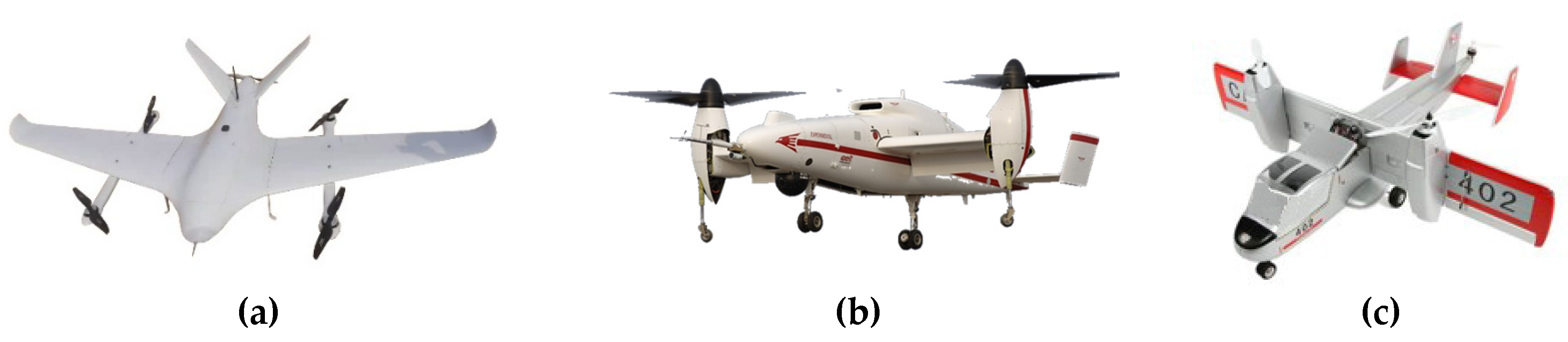
Figure 2.
Pitch-decoupled VTOL UAV with a robotic arm.
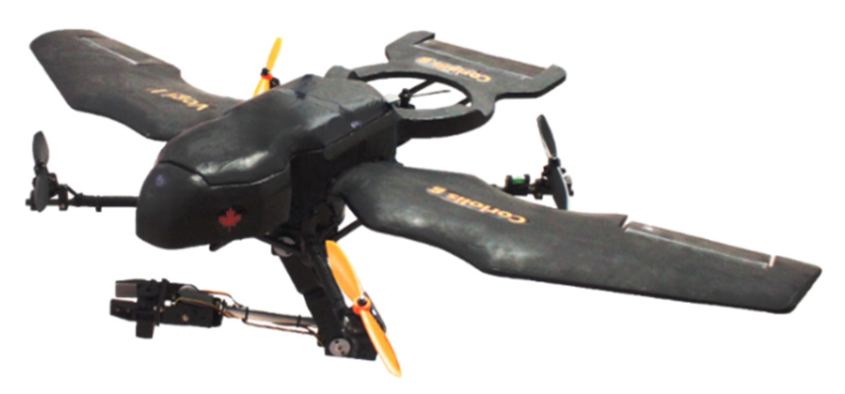
Figure 3.
Mechanical design of a pitch-decoupled VTOL UAV: (a) takeoff and landing modes, (b) horizontal-flight mode.
Figure 3.
Mechanical design of a pitch-decoupled VTOL UAV: (a) takeoff and landing modes, (b) horizontal-flight mode.
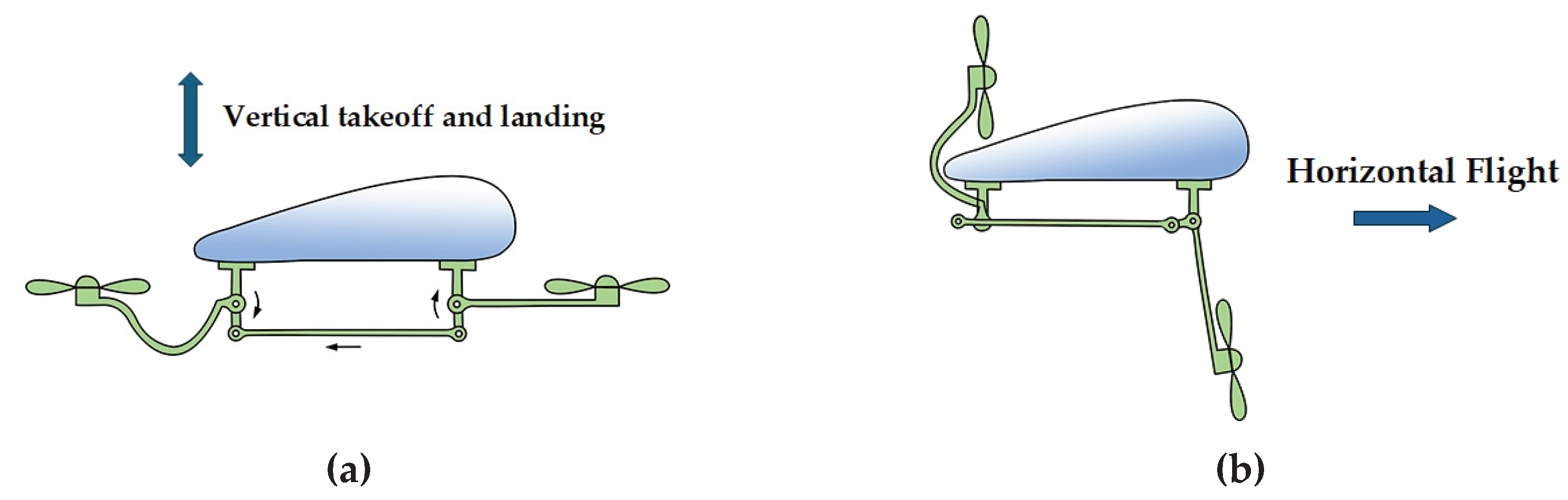
Figure 4.
Kinematic model of the pitch-decoupled VTOL UAV with an attached robotic arm.
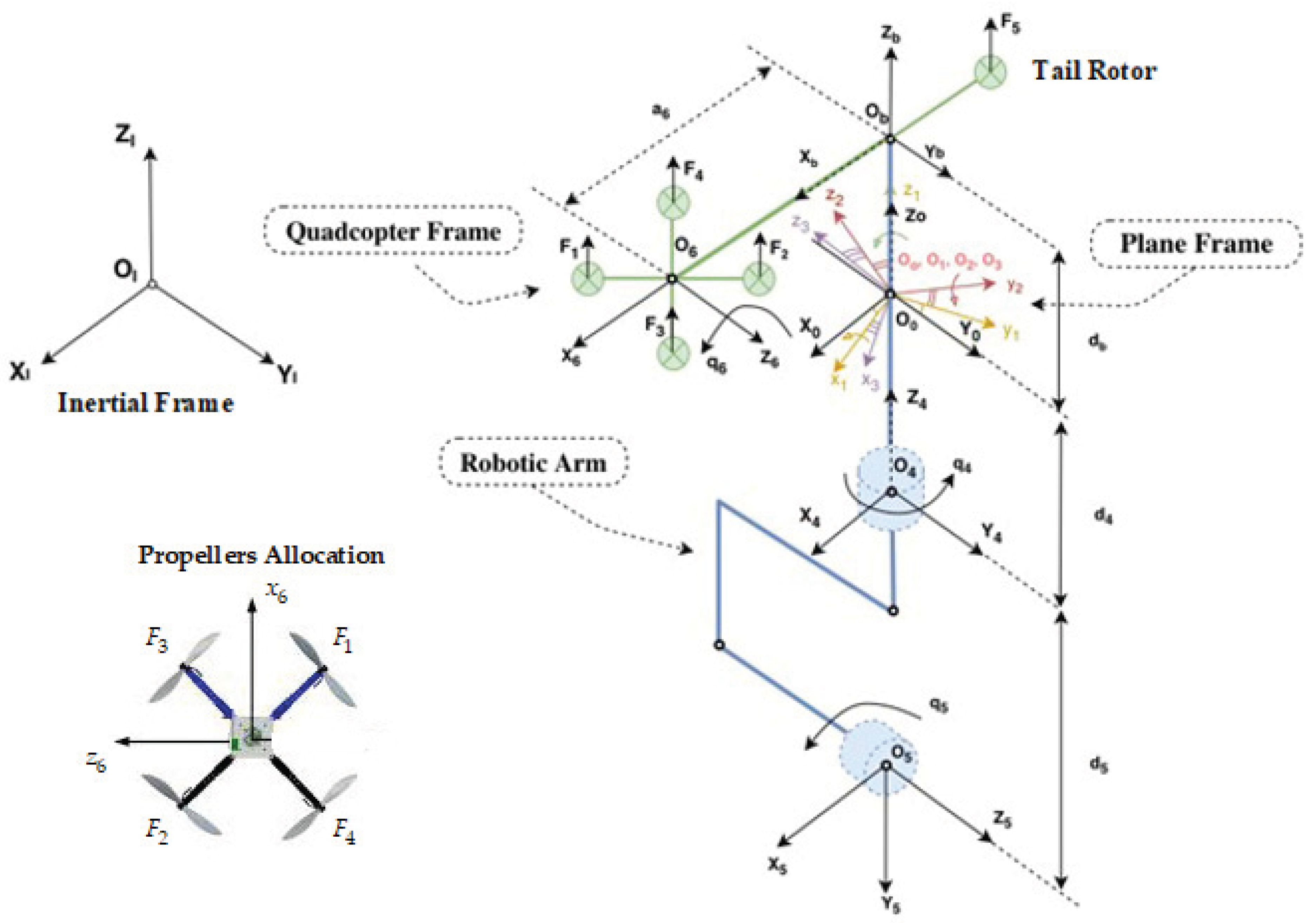
Figure 5.
Schematic block diagram of kinematic links of the pitch-decoupled UAV.
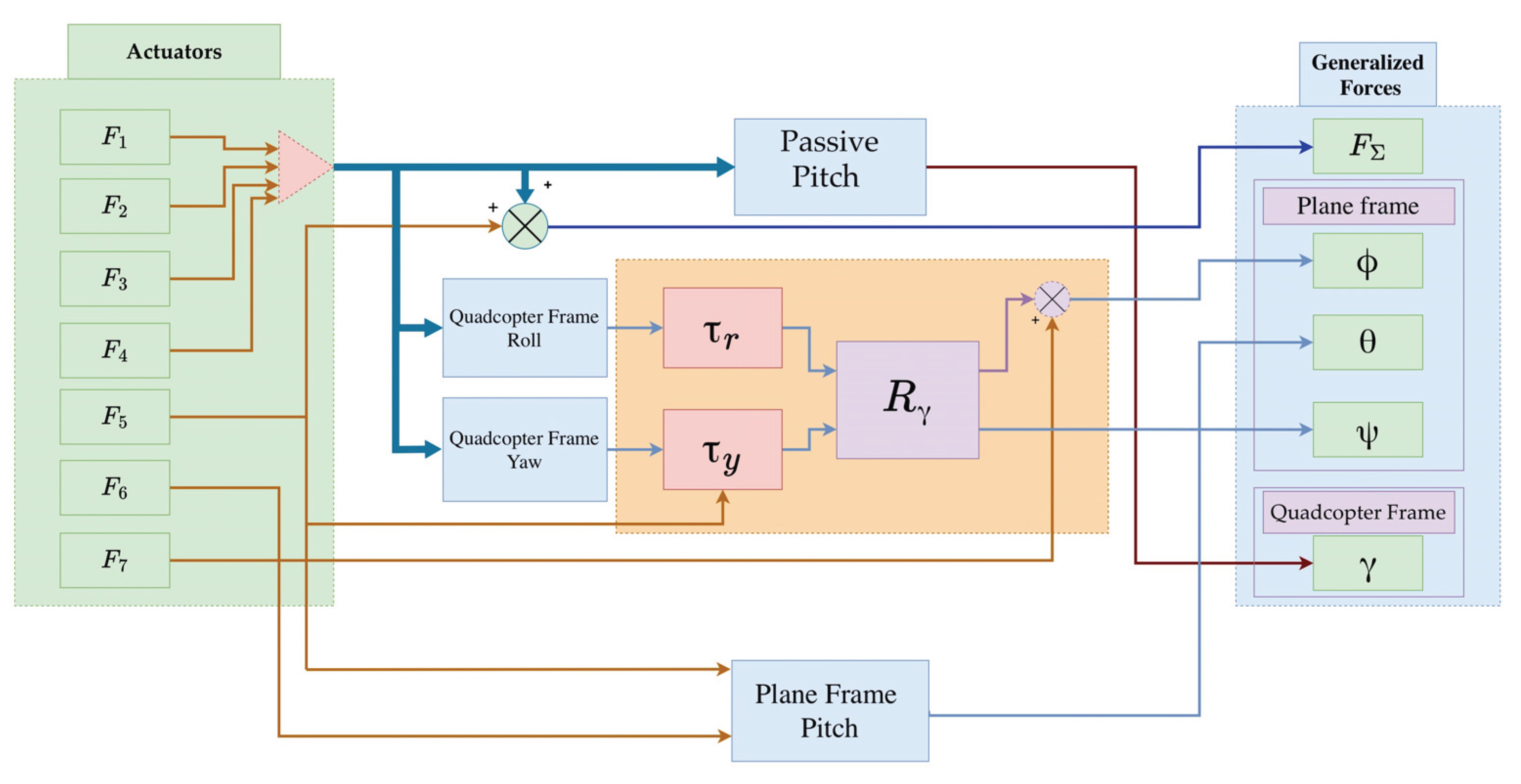
Figure 5.
Forces acting on the pitch-decoupled UAV during horizontal flight () .
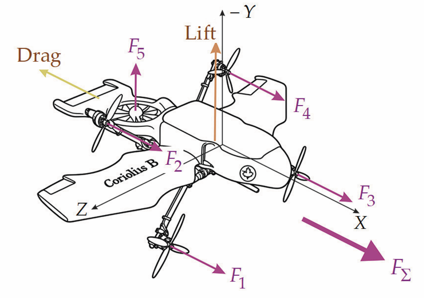
Figure 6.
Aerodynamic coefficients of the pitch-decoupled UAV obtained for different simulation runs; (a) over , (b) versus ; (d) versus ; (d) versus .
Figure 6.
Aerodynamic coefficients of the pitch-decoupled UAV obtained for different simulation runs; (a) over , (b) versus ; (d) versus ; (d) versus .
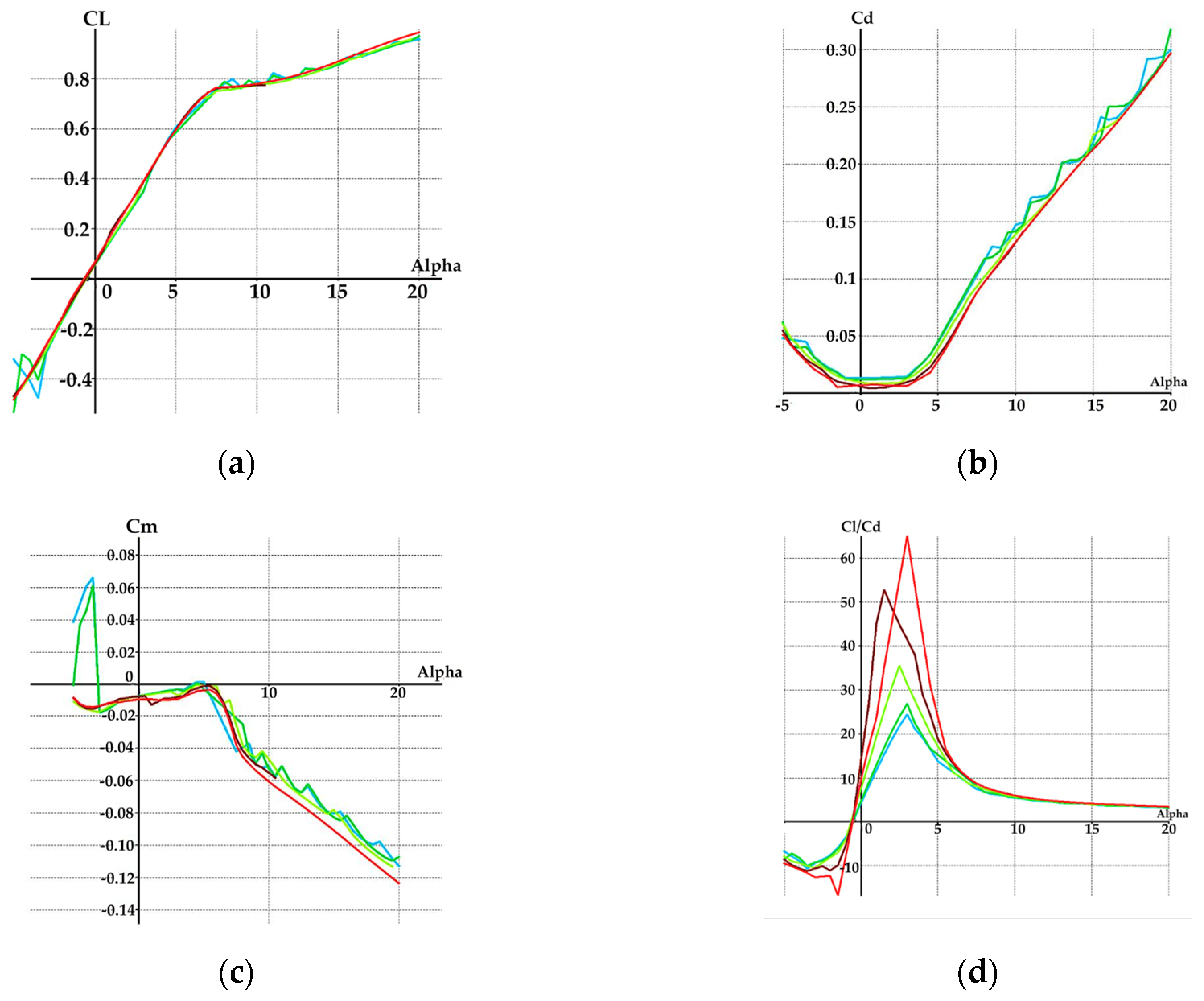
Figure 7.
Aerodynamic stability analysis of the UAV: (a) lateral axis, (b) longitudinal axis.
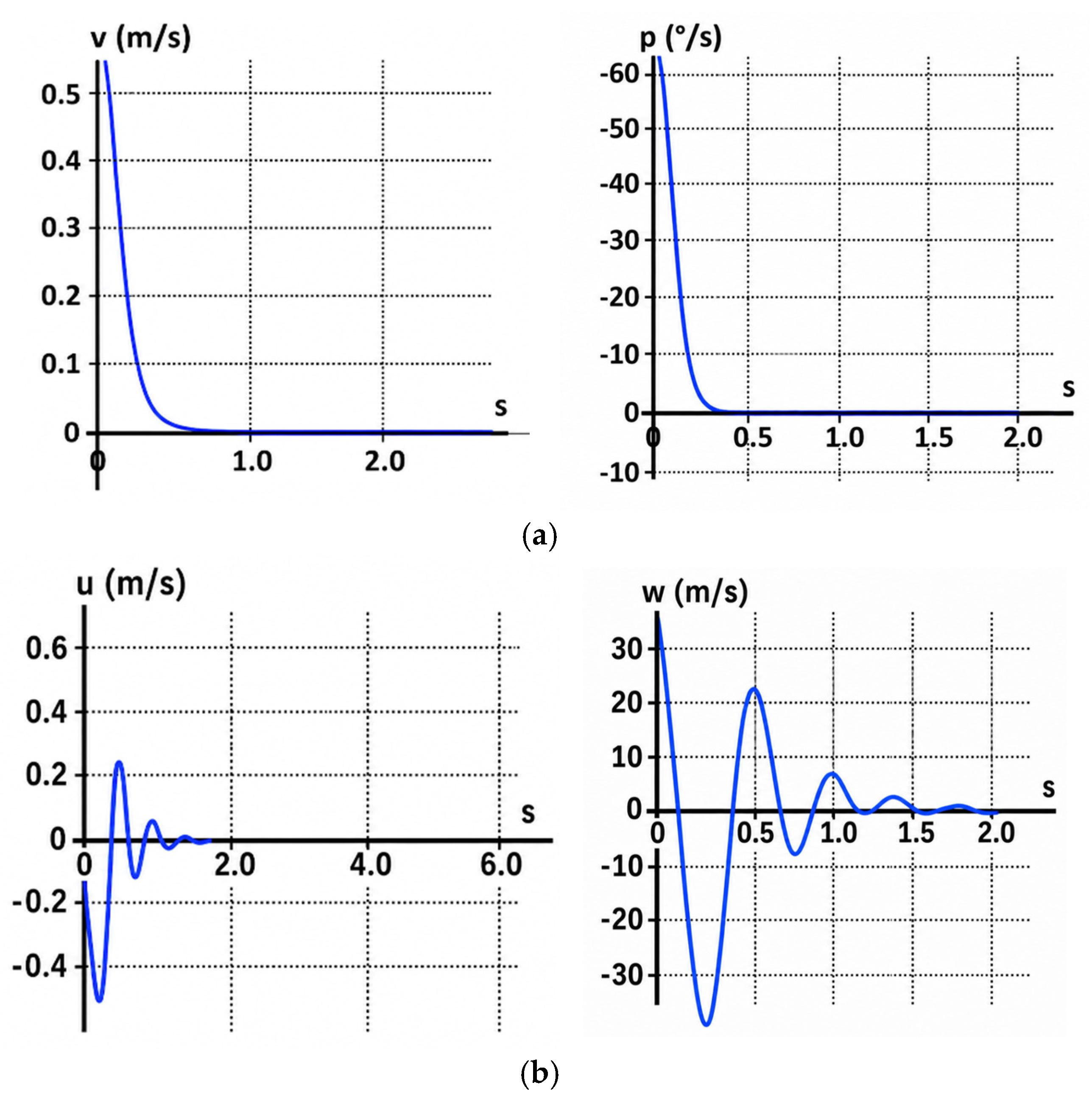
Figure 8.
Illustration of the “sloped” mode: (a) horizontal flight, (b) climb flight.
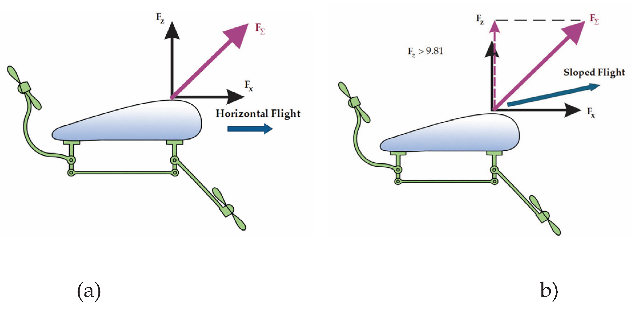
Figure 9.
Matrix block diagram of the control system of the pitch-decoupled UAV with the robotic arm in hover mode.
Figure 9.
Matrix block diagram of the control system of the pitch-decoupled UAV with the robotic arm in hover mode.
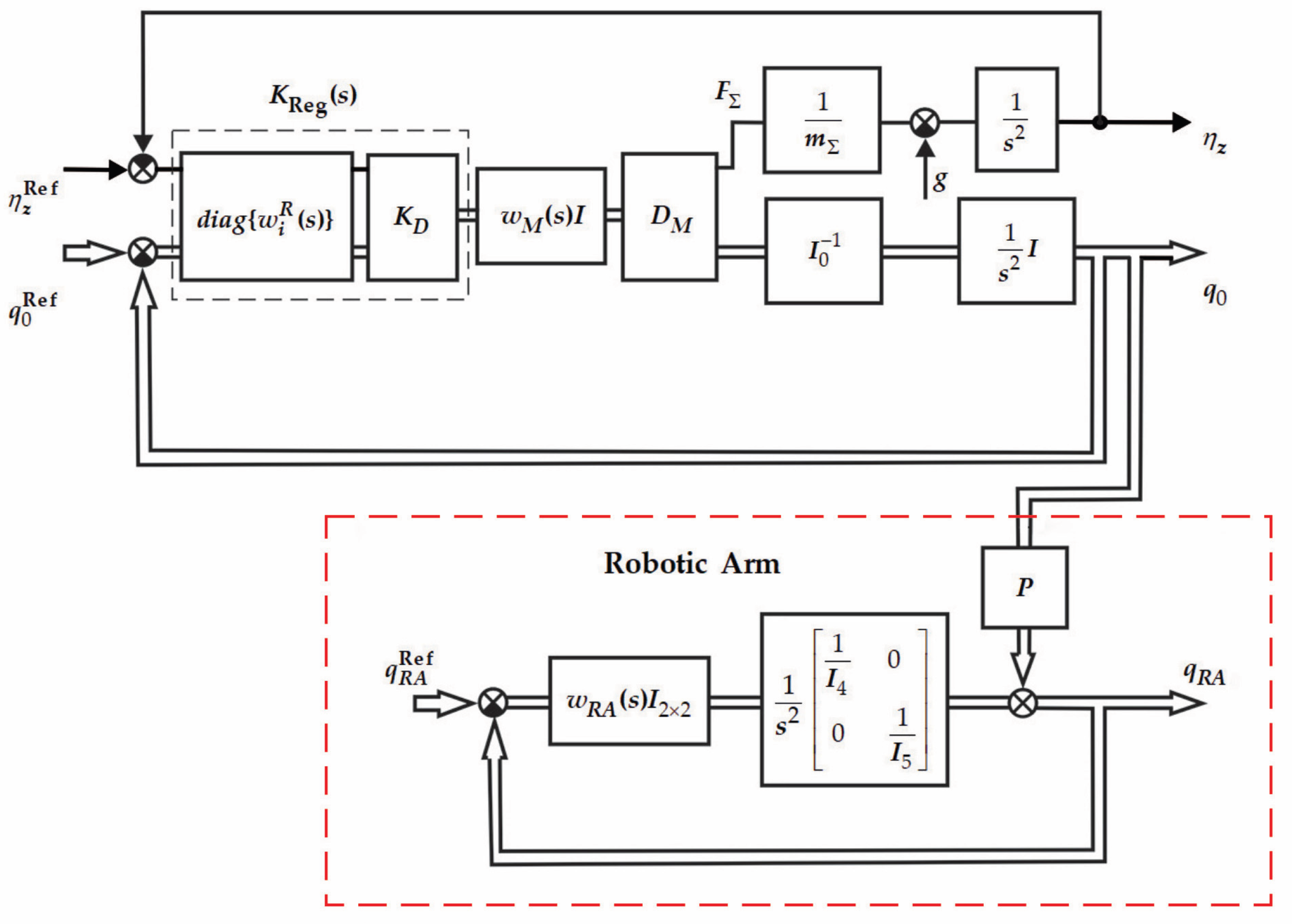
Figure 10.
Step responses of the pitch-decoupled UAV with the robotic arm: (a) roll, pitch, and yaw axes; (b) rotation angles of the robot’s links.
Figure 10.
Step responses of the pitch-decoupled UAV with the robotic arm: (a) roll, pitch, and yaw axes; (b) rotation angles of the robot’s links.
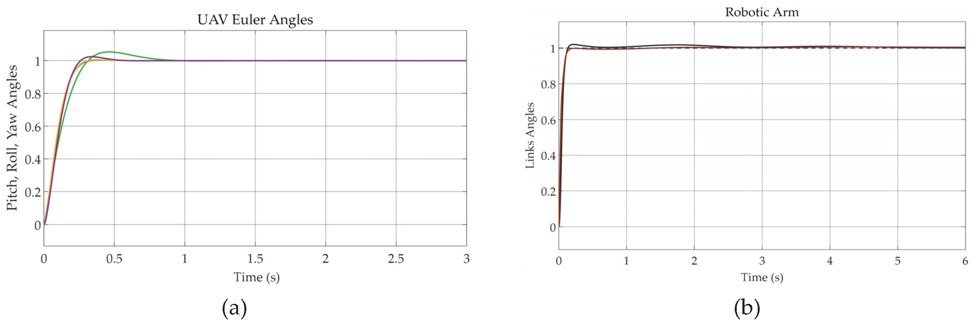
Figure 11.
Matrix block diagram of the control system of the pitch-decoupled UAV in the transition modes.
Figure 11.
Matrix block diagram of the control system of the pitch-decoupled UAV in the transition modes.
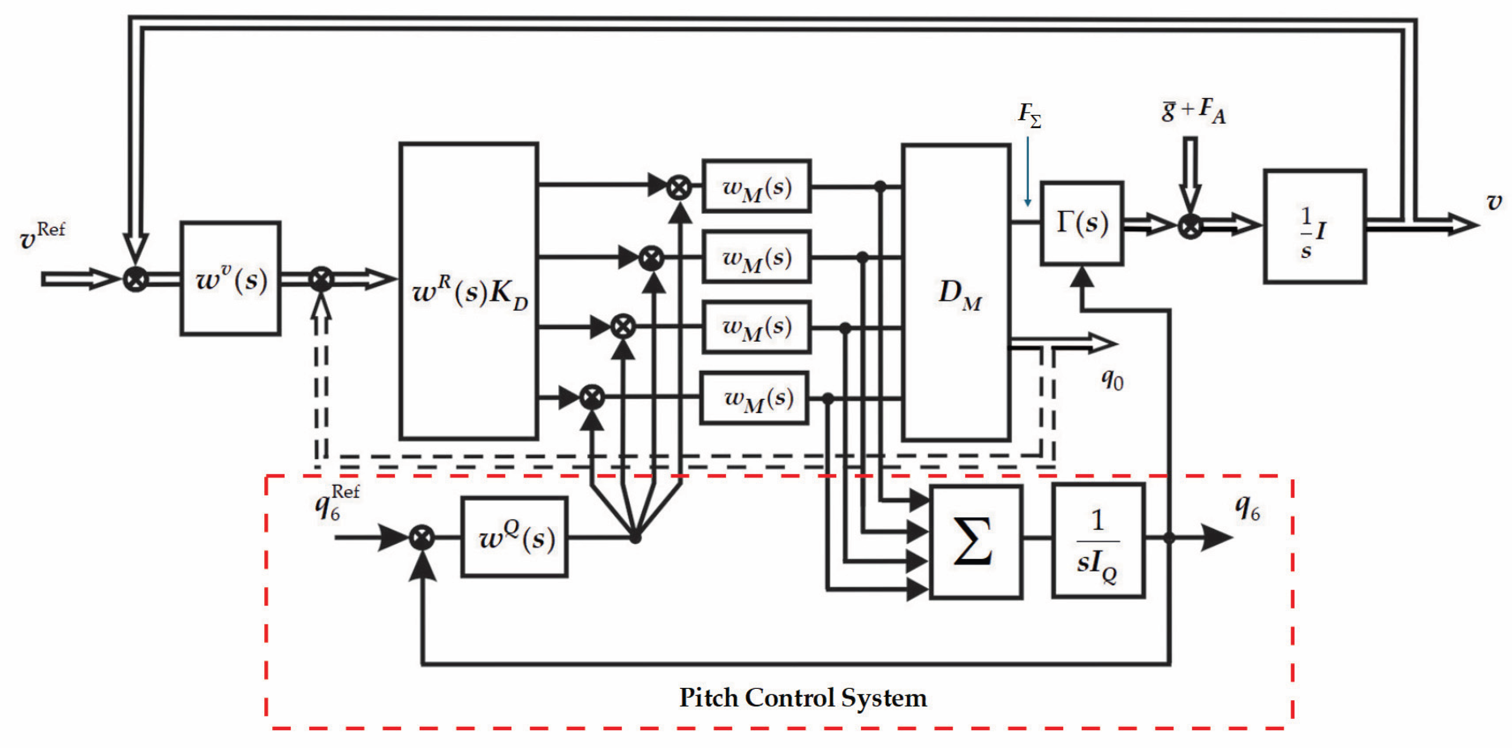
Figure 12.
Transition phase simulation (): 3D simulation.
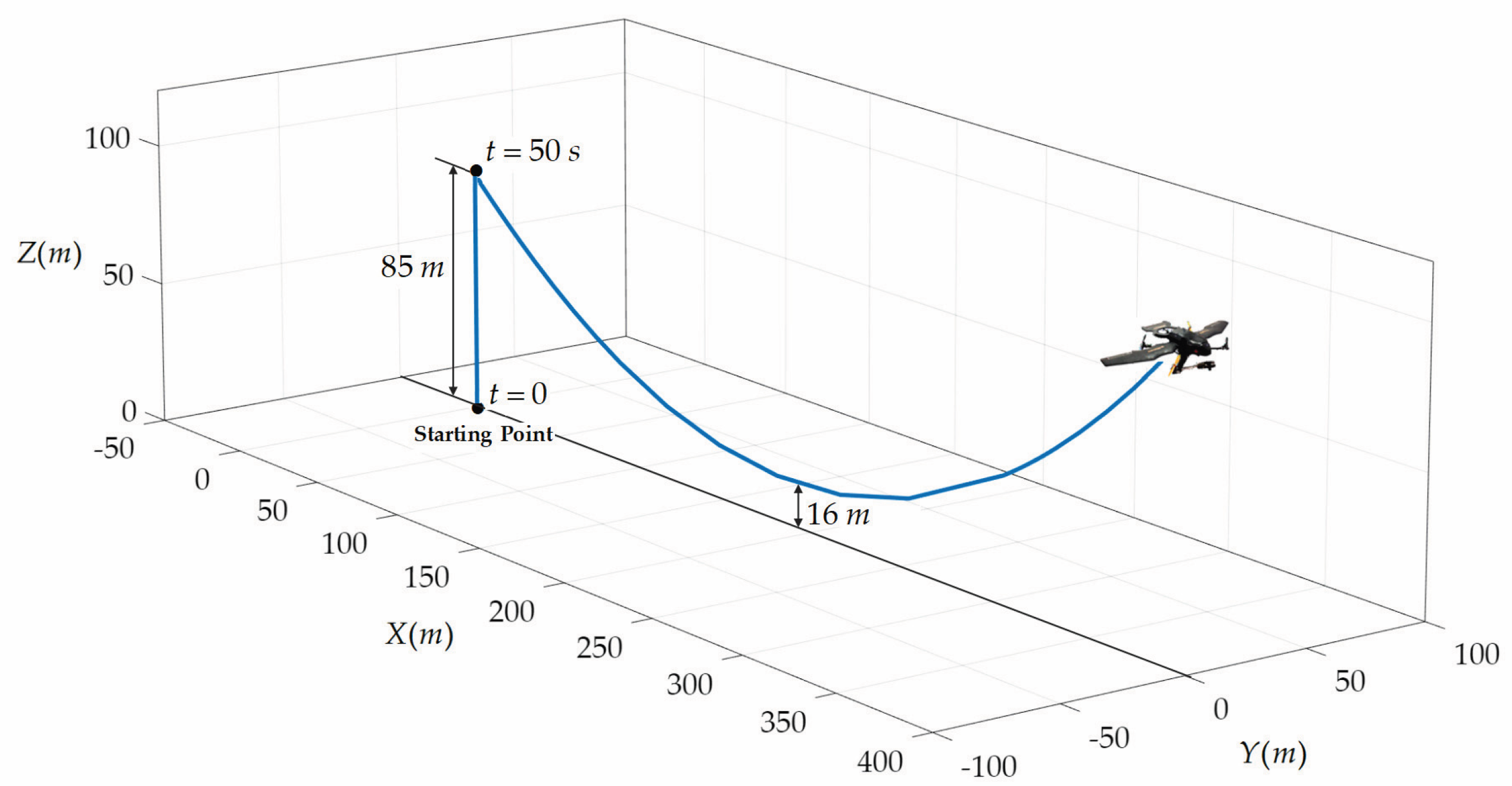
Figure 13.
Transition phase simulation (): and altitude response graphs.
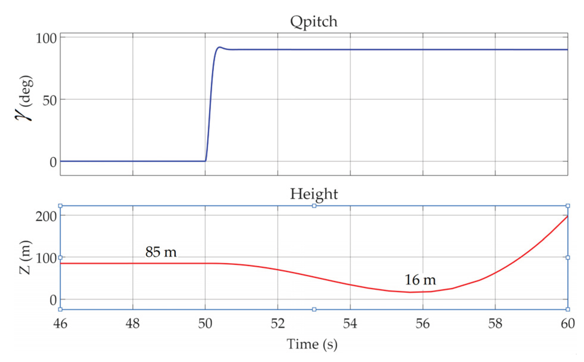
Figure 14.
Transition phase simulation (): and altitude response graphs.
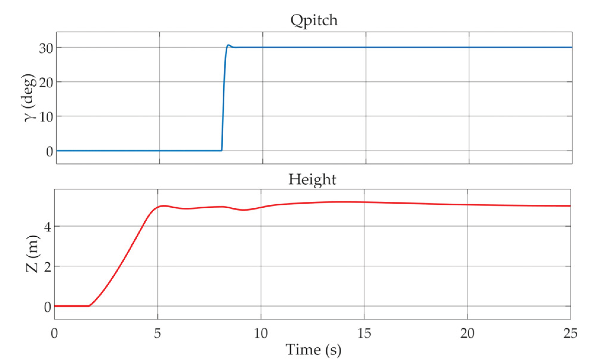
Figure 15.
Transition phase simulation (): horizontal velocity and aerodynamic forces.
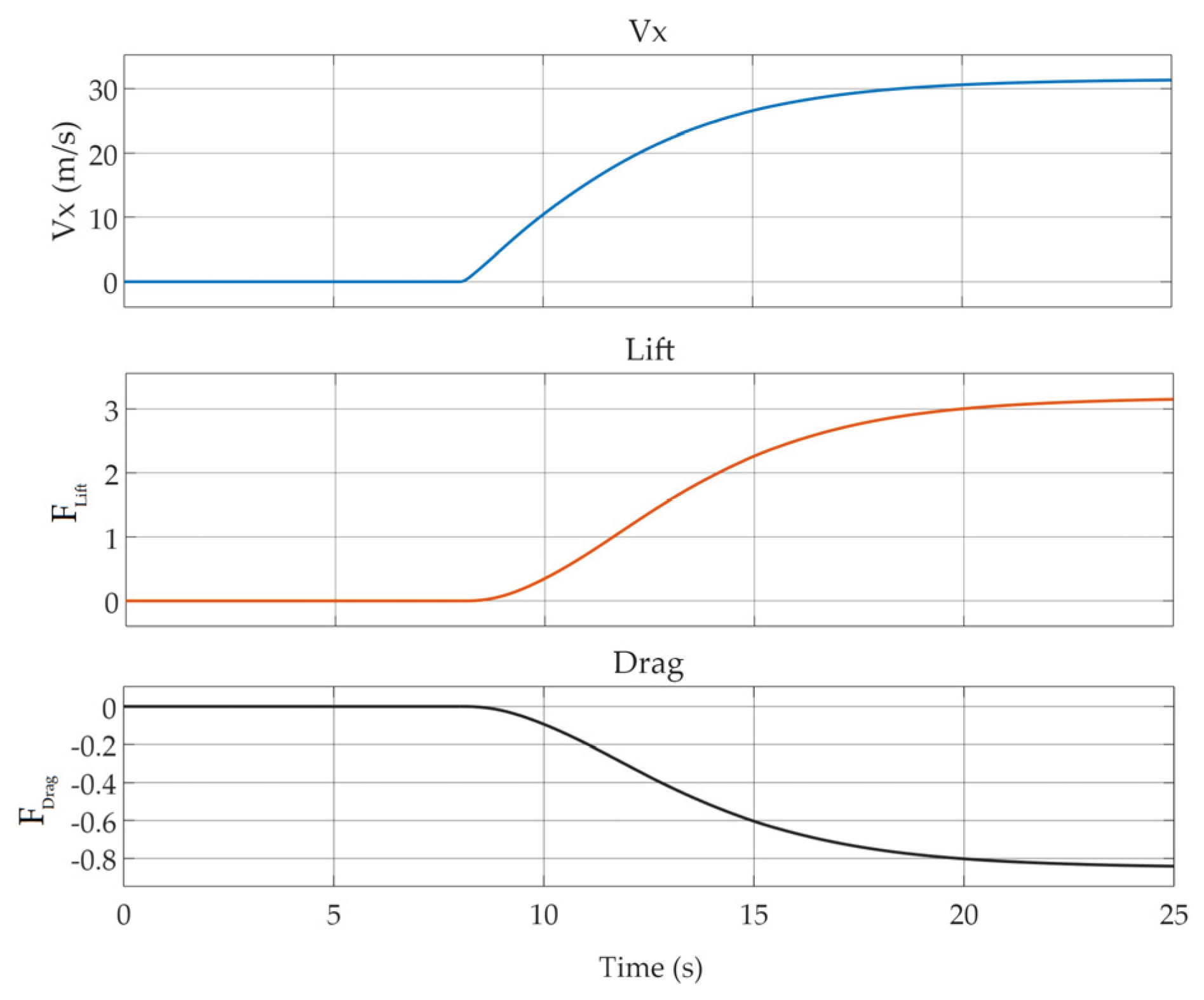
Figure 16.
Transition phase simulation (): total thrust change.
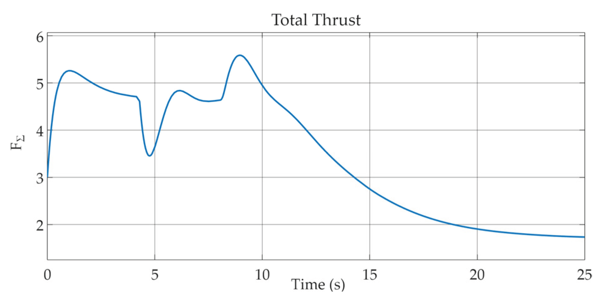
Figure 17.
Actor-critic diagram implemented for the pitched-decoupled UAV training.
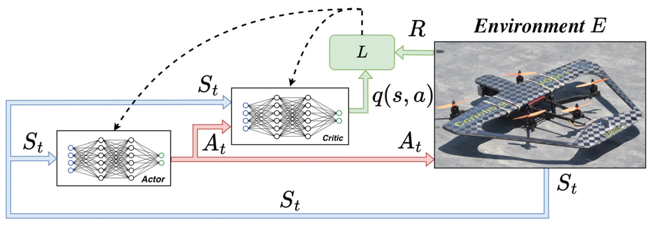
Figure 18.
Block diagram of the VTOL UAV control system with the neural controller.
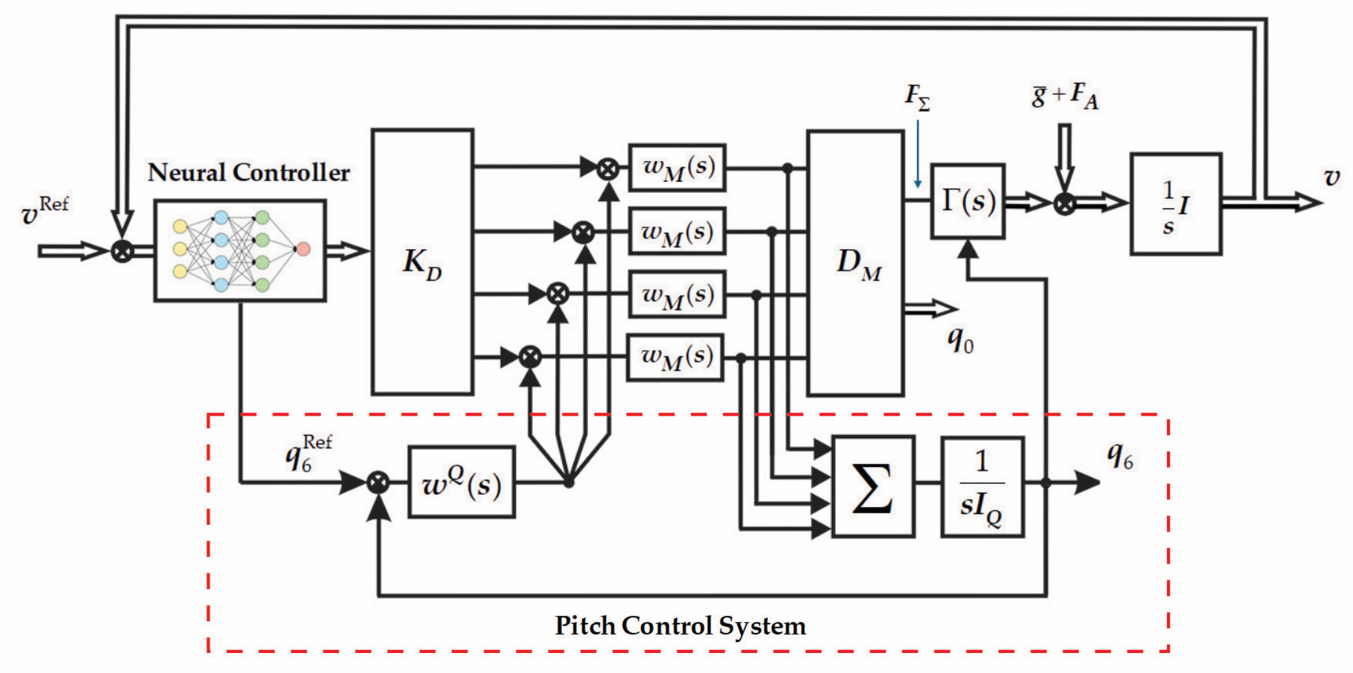
Figure 19.
Training process over episodes.
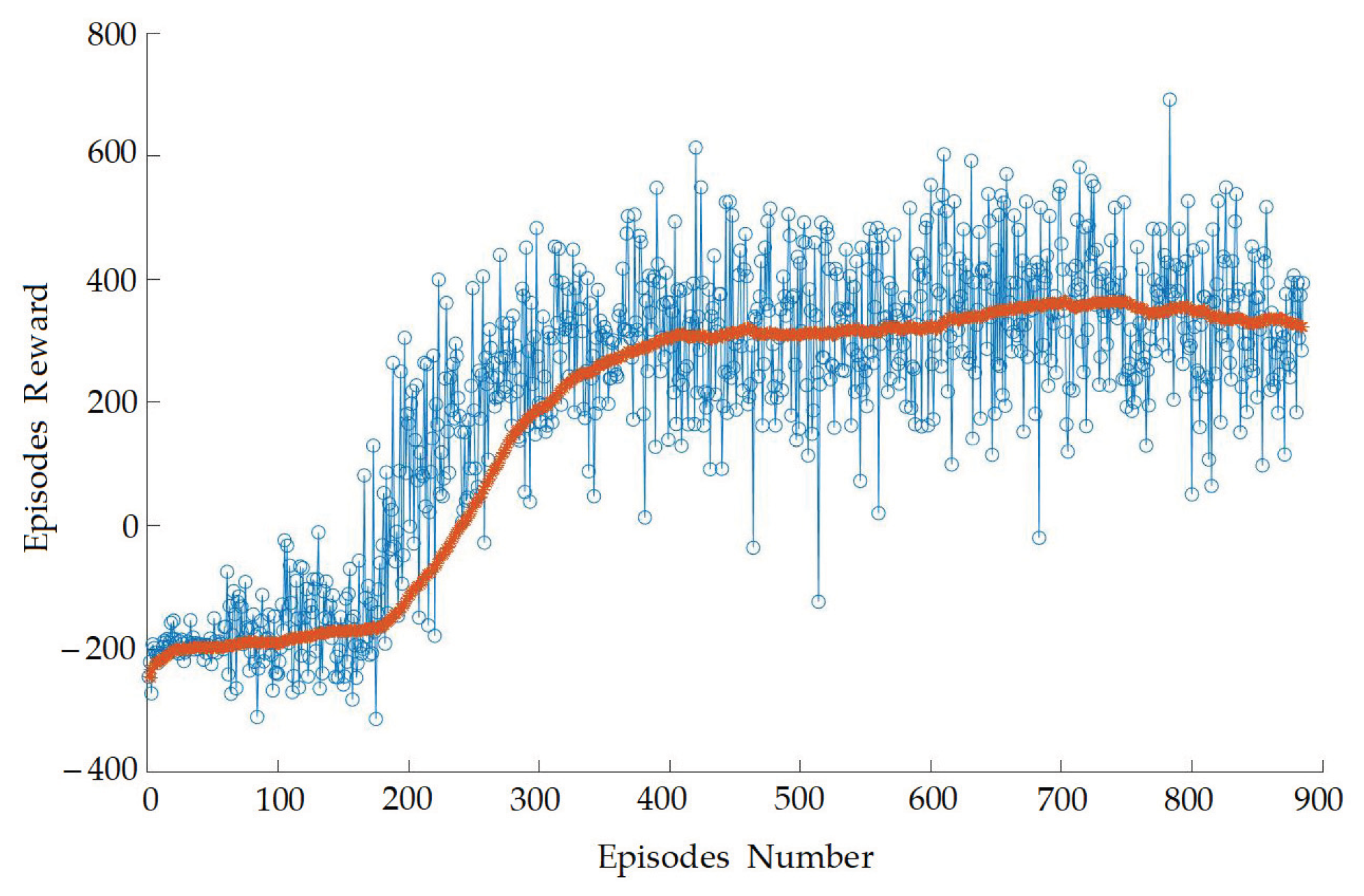
Figure 20.
Transition-phase simulation for Scenario 1: and altitude response graphs.
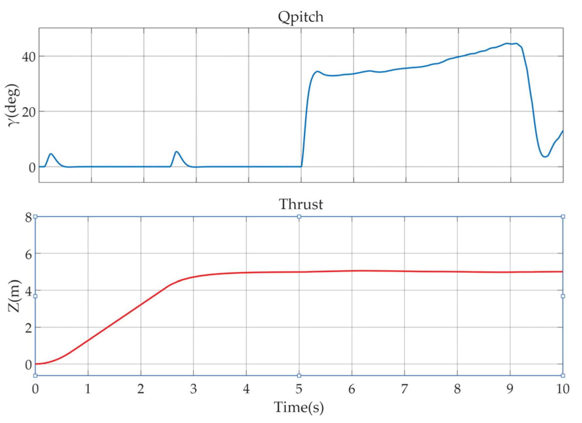
Figure 21.
Transition phase simulation for Scenario 1: horizontal and vertical velocities.
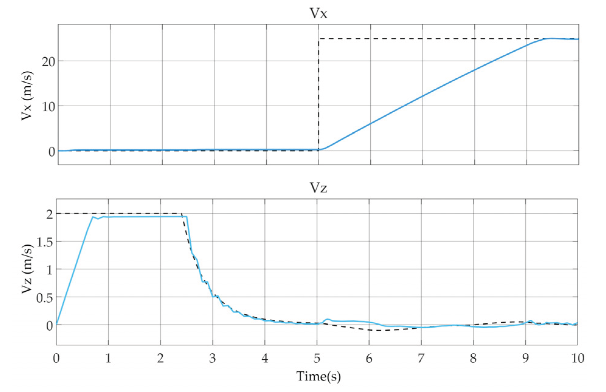
Figure 22.
Transition phase simulation for Scenario 2: and altitude response graphs.
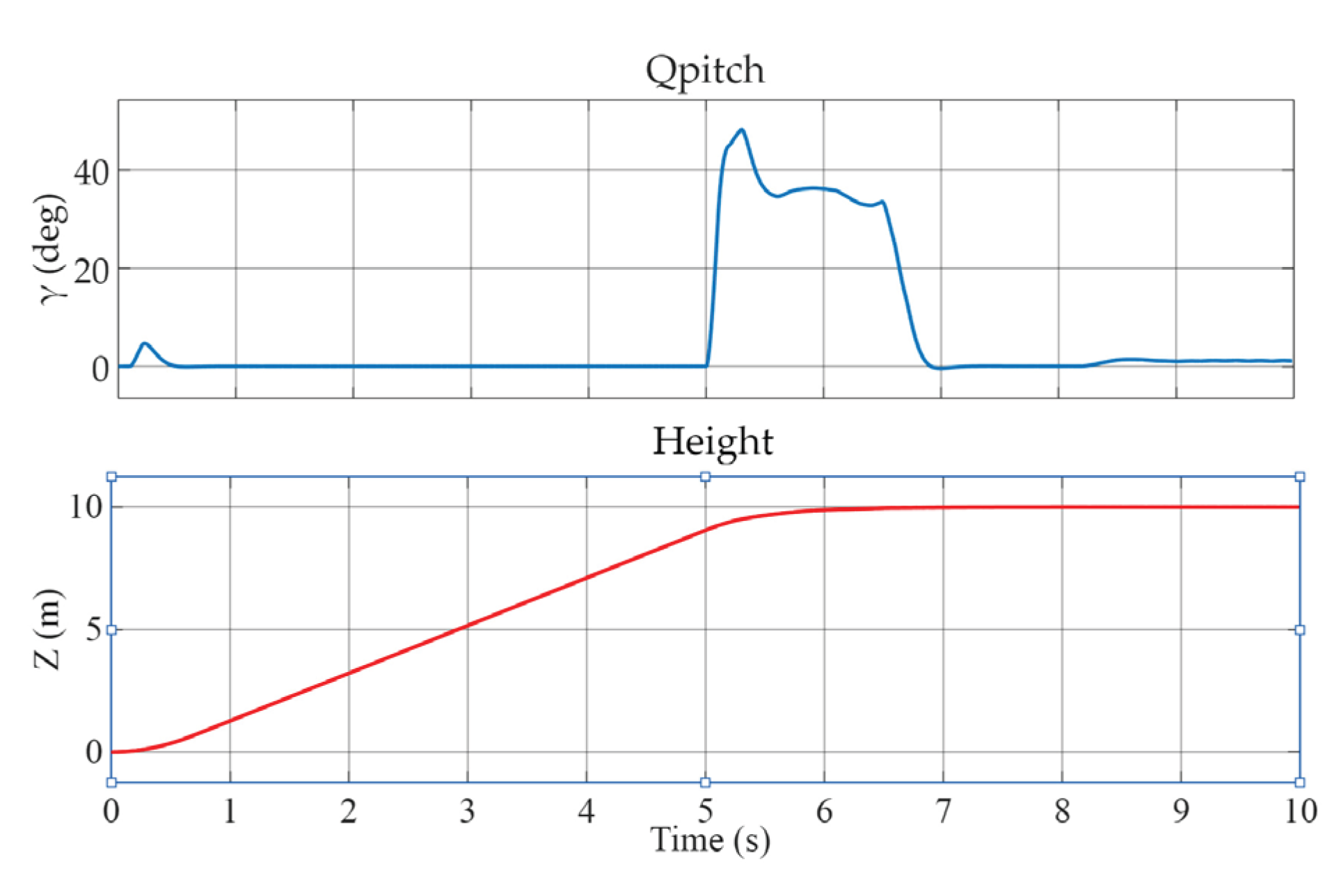
Figure 23.
Transition phase simulation for Scenario 2: horizontal and vertical velocities.
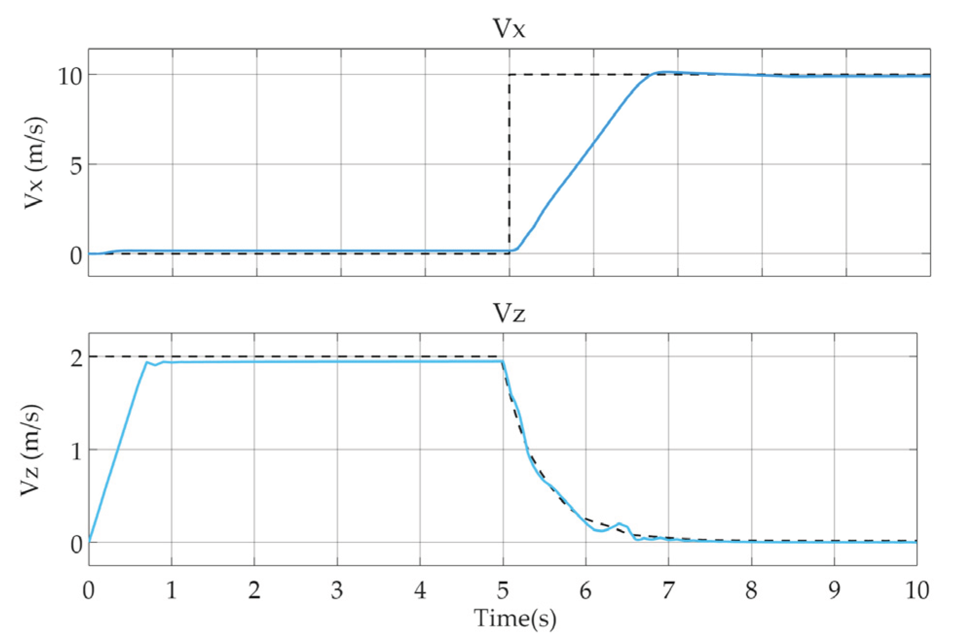
Figure 24.
Simplified matrix block diagram of the control system of the pitch-decoupled UAV.
Disclaimer/Publisher’s Note: The statements, opinions and data contained in all publications are solely those of the individual author(s) and contributor(s) and not of MDPI and/or the editor(s). MDPI and/or the editor(s) disclaim responsibility for any injury to people or property resulting from any ideas, methods, instructions or products referred to in the content. |
© 2026 by the authors. Licensee MDPI, Basel, Switzerland. This article is an open access article distributed under the terms and conditions of the Creative Commons Attribution (CC BY) license (http://creativecommons.org/licenses/by/4.0/).
Copyright: This open access article is published under a Creative Commons CC BY 4.0 license, which permit the free download, distribution, and reuse, provided that the author and preprint are cited in any reuse.


