

Submitted:
08 August 2026
Posted:
11 August 2026
You are already at the latest version
Abstract
Acoustic and image sensors in unattended ground sensor systems often operate with different sampling rates, trigger mechanisms, and fields of view, so their observations are asynchronous and lack instance-level correspondence. In addition, web images used to supplement scarce field annotations exhibit a substantial domain shift from target-domain images. This paper proposes a three-stream joint learning framework that integrates reliability-weighted image-domain adaptation, reliability-aware dynamic bidirectional prototype distillation, and balanced complementary modality dropout. A lightweight shared backbone processes labeled acoustic spectra, labeled mixed-source images, and unlabeled target-domain images. Target pseudo-label reliability is estimated by a main classifier and two auxiliary classifiers and is used to weight marginal and class-conditional distribution alignment. Acoustic and image class prototypes transfer category-level knowledge without constructing artificial instance pairs, while direction-specific distillation weights are dynamically assigned according to classification reliability, prototype availability, and prototype stability. Experiments on 148,038 acoustic spectra and 167,754 images yield acoustic, image, and overall accuracies of 92.02\%, 95.26\%, and 93.79\%, respectively, exceeding the best corresponding baseline results by 1.49, 1.24, and 2.47 percentage points. The deployment model contains 123.40 K parameters and requires 0.47 MiB in FP32, supporting resource-constrained field deployment.
Keywords:
unattended ground sensors
; moving ground target classification
; asynchronous multimodal learning
; domain adaptation
; prototype knowledge distillation
; acoustic–image learning
; edge intelligence
1. Introduction
Unattended ground sensor (UGS) systems provide persistent, covert, and distributed monitoring for moving ground targets. Acoustic sensors offer low-cost, wide-area, and all-weather observations, whereas image sensors provide visually interpretable appearance cues with strong discriminative value. Combining these heterogeneous sensing channels can improve target classification reliability in field environments [1,2]. However, practical acoustic–image UGS systems differ substantially from conventional synchronized audio–visual datasets. Acoustic and image sensors commonly use different sampling rates, trigger rules, sensing ranges, and fields of view. Their observations therefore cannot be assumed to form temporally aligned or instance-level paired samples.
The image branch also faces a severe data limitation. Although field videos can provide UGS image frames, consecutive frames are highly correlated and cover only a limited range of scenes, target instances, and environmental conditions. Public web images can expand the labeled training set, but the resulting source-side images differ from target UGS images in viewpoint, scale, illumination, background, and acquisition conditions. Such dataset bias and distribution shift can substantially reduce generalization performance [3,4,5]. Consequently, the learning problem involves two coupled challenges: image-domain adaptation from labeled mixed-source images to unlabeled UGS images, and cross-modal knowledge transfer between non-paired acoustic and image samples.
Existing domain adaptation methods reduce source–target discrepancy by statistical distribution matching or adversarial learning [6,7,8,9]. These methods are effective for image-domain transfer but do not explicitly exploit category-level acoustic–image complementarity. Conversely, multimodal alignment and cross-modal distillation methods can associate heterogeneous representations [10,11,12], but most assume paired or weakly paired observations and rarely address simultaneous image-domain shift. Moreover, fixed and symmetric knowledge transfer can propagate unreliable information when the two modalities converge at different rates or contain unequal class evidence.
To address these limitations, this paper develops an asynchronous acoustic–image joint learning framework that learns from three independently sampled data streams: labeled acoustic spectra, labeled mixed-source images, and unlabeled target-domain UGS images. The method combines reliability-weighted image-domain alignment with category-level bidirectional prototype distillation and a balanced complementary modality dropout strategy. The main contributions are as follows:
- A three-stream shared learning architecture is formulated for asynchronous and non-paired acoustic–image observations. It jointly handles labeled acoustic data, labeled mixed-source images, and unlabeled target images without constructing instance-level acoustic–image pairs.
- A reliability-weighted two-stage image-domain adaptation mechanism is introduced. Multi-classifier consensus estimates target pseudo-label reliability, which weights both marginal distribution alignment and class-conditional alignment.
- A reliability-aware dynamic bidirectional prototype distillation mechanism is proposed. Direction-specific transfer strengths are determined from teacher classification reliability, prototype availability, and prototype stability, reducing negative transfer caused by fixed symmetric distillation.
- A balanced complementary modality dropout mechanism regularizes the shared backbone while preserving equal marginal retention probabilities for both modalities and preventing simultaneous removal of the two labeled streams. The complete method attains 93.79% overall accuracy with a compact 123.40 K-parameter deployment network.
2. Related Work
2.1. UGS Target Classification and Multimodal Sensing
UGS target classification traditionally relies on acoustic, seismic, passive infrared, magnetic, or image observations. Acoustic sensing is attractive because it can capture engine, track, tire, and footstep signatures at relatively low deployment cost. Image sensing provides complementary shape and appearance cues, but its performance is affected by illumination, occlusion, background complexity, and viewing distance. Earlier UGS studies demonstrated that combining heterogeneous sensing modalities can improve target recognition compared with single-sensor decisions [1,2]. More generally, multimodal learning aims to exploit complementary information through feature-, representation-, or decision-level interaction [13,14].
Most multimodal architectures are developed for synchronized or naturally paired samples, such as audio–visual events, image–text pairs, or multimodal sentiment sequences [15,16,17]. In distributed UGS deployments, however, an acoustic record and an image crop with the same category label may originate from different targets, locations, and collection times. Direct concatenation or pairwise contrastive learning can therefore introduce false instance correspondence. This study instead treats class labels as the only common semantic anchor and performs category-level transfer through modality-specific prototype memories.
2.2. Domain Adaptation for Field Images
Domain adaptation seeks to learn transferable representations when training and test data follow different distributions [6]. The Deep Adaptation Network (DAN) minimizes multi-kernel maximum mean discrepancy (MK-MMD), a kernel distance between distributions [7,18]. Domain-Adversarial Neural Networks (DANN) use a gradient reversal layer and domain discriminator to obtain domain-invariant features [8]. Conditional Adversarial Domain Adaptation (CDAN) incorporates classifier predictions into domain alignment to reduce category mismatch [9]. Minimum Class Confusion (MCC) improves target discrimination by reducing inter-class ambiguity [19]. Semi-supervised methods such as MME and TriCT additionally exploit a small number of labeled target samples [20,21].
Global distribution alignment alone can mix samples from different categories, whereas class-conditional alignment depends on reliable target pseudo-labels. Self-training studies have shown both the utility of target pseudo-labels and the need to control class imbalance and label noise [22]. In realistic field imagery, early pseudo-labels are noisy because of background and viewpoint shifts. The proposed method therefore estimates per-sample reliability from confidence and agreement among three classifiers and progressively activates global and conditional alignment losses.
2.3. Cross-Modal Knowledge Transfer
Cross-modal learning transfers semantic information across heterogeneous observation spaces. Early cross-modal distillation transferred intermediate supervision between paired sensing modalities [23]. Meta-alignment methods learn cross-modal generalization under low-resource conditions [10]; geometric multimodal contrastive learning aligns modality representations using cross-modal relationships [11]; and XKD combines domain alignment with cross-modal knowledge distillation for video representation learning [12]. Knowledge distillation commonly transfers softened outputs or intermediate representations from a teacher to a student [24], while prototypical and center-based learning represent each class by a compact feature centroid [25,26].
For non-paired UGS data, class prototypes provide a natural semantic bridge because they do not require instance synchronization. Nevertheless, the acoustic and image branches can have different noise levels and convergence dynamics. Treating both modalities as equally reliable teachers at every epoch is therefore suboptimal. The proposed method explicitly estimates teacher reliability and dynamically allocates a fixed total distillation budget between the two transfer directions.
3. Materials and Methods
3.1. Problem Formulation
Let the labeled acoustic dataset be
where is an acoustic power spectral density image and . The labeled mixed-source image domain is
which contains web images and a small subset of labeled UGS images. The unlabeled target domain is
The three datasets share the same category set but contain no temporal or instance-level correspondence. In each iteration, mini-batches are independently sampled from
which prevents the model from relying on artificial acoustic–image pairings.
The task is to learn a shared feature extractor and classifier that correctly classify acoustic samples and target-domain UGS images. During inference, each acoustic or image sample is processed independently; simultaneous availability of both modalities is not required.
3.2. Datasets and Preprocessing
3.2.1. Acoustic Data
The acoustic data contain pedestrian, tracked-vehicle, and wheeled-vehicle observations collected by a UGS acoustic array. To maintain a consistent single-node input configuration, only the first acoustic channel is used. Each waveform is divided into one-second windows containing 1024 samples. A short-time Fourier transform is applied to obtain a power spectral density representation [28], which is cropped, normalized, and resized to a grayscale spectrum.
The acoustic dataset is divided using stratified group splitting with an approximate ratio of 8:1:1. Windows from the same original recording are assigned to only one subset to prevent near-duplicate leakage. Table 1 summarizes the resulting 148,038 acoustic samples.
3.2.2. Image Data
UGS images are extracted from field videos collected at target distances of approximately 20–200 m during the day and at night, with grass, gravel, cement, and hard soil as backgrounds. Figure 1 shows representative deployment environments and field-collected observations, illustrating the long sensing distances, complex backgrounds, varying illumination conditions, and small apparent target sizes encountered in practical UGS operation. Target bounding boxes are annotated and cropped from 13,012 original frames with a resolution of . The cropped images are resized with aspect-ratio-preserving padding and converted to grayscale images. The UGS subset contains 47,706 target crops: 15,746 pedestrian, 16,681 tracked-vehicle, and 15,279 wheeled-vehicle images.
To improve source-side diversity, 120,048 labeled web images are added, including 39,640 pedestrian, 40,240 tracked-vehicle, and 40,168 wheeled-vehicle samples. The final image dataset contains 167,754 samples. A small labeled UGS subset is combined with the web images to form the labeled mixed-source domain ; the remaining UGS training images form the unlabeled target domain . UGS videos are grouped before splitting so that frames from one video do not cross training, validation, and test subsets. Table 2 gives the detailed distribution.
Figure 2 illustrates the heterogeneous acoustic and image inputs and their shared category-level, rather than instance-level, correspondence.
3.3. Overview of the Proposed Framework
Figure 3 presents the complete framework. Three streams independently process acoustic spectra A, labeled mixed-source images , and unlabeled target images . They share convolutional and classifier parameters but use modality-dependent batch normalization: the acoustic stream has independent batch-normalization statistics, whereas the two image streams share image-domain statistics. Related domain-specific batch-normalization designs separate low-level domain statistics while sharing the remaining network parameters [29]. This design retains a common semantic space while avoiding direct mixing of acoustic and image feature distributions at normalization layers.
The framework contains three interacting mechanisms. First, reliability-weighted maximum mean discrepancy and class-wise conditional MMD align source and target image distributions. Second, acoustic and image class-prototype memories establish category-level cross-modal transfer. Third, balanced complementary modality dropout regularizes the labeled acoustic and image residual paths. The unlabeled target stream remains active to preserve stable domain alignment.
Figure 3.
Overall architecture of the proposed asynchronous acoustic–image joint learning framework. Acoustic, labeled mixed-source image, and target-image samples are independently drawn and processed by a shared lightweight backbone.
Figure 3.
Overall architecture of the proposed asynchronous acoustic–image joint learning framework. Acoustic, labeled mixed-source image, and target-image samples are independently drawn and processed by a shared lightweight backbone.
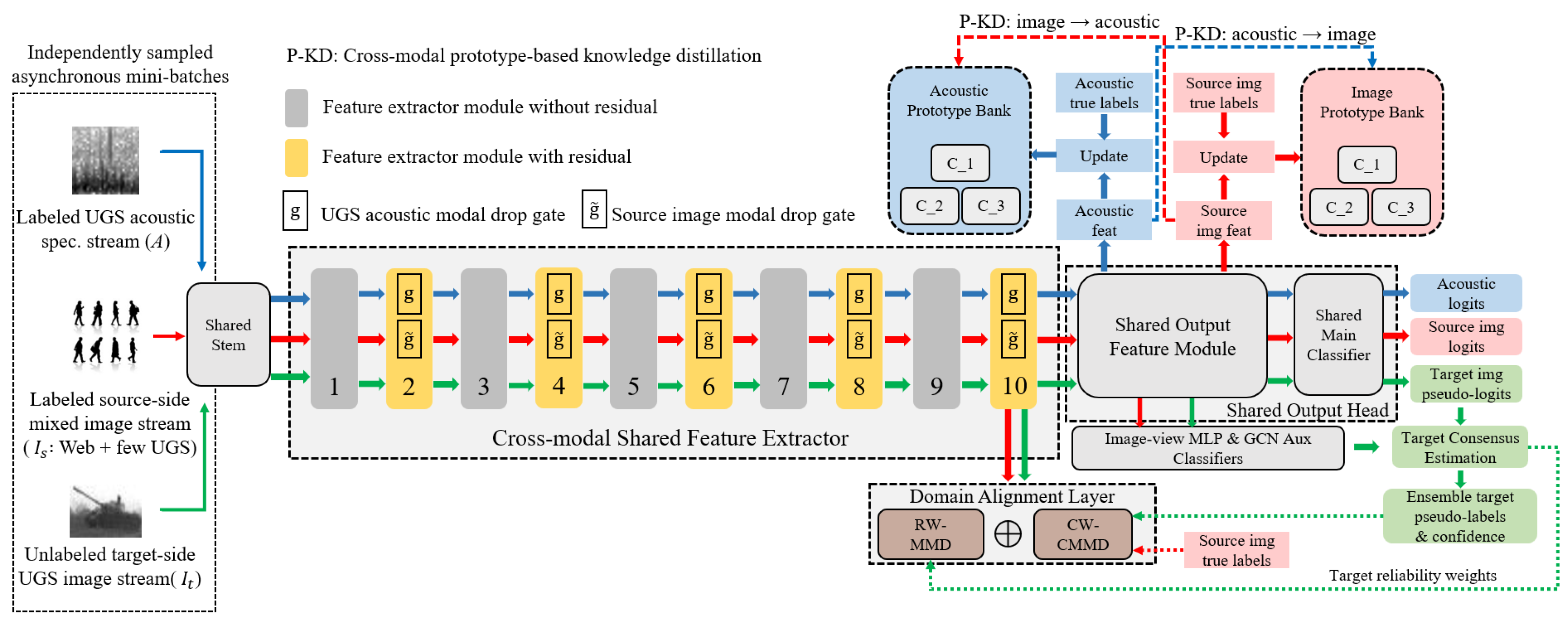
3.4. Shared Lightweight Backbone
The shared feature extractor follows an inverted-residual design inspired by MobileNetV2 [30]. All inputs have one channel and a spatial size of . A stem convolution is followed by ten inverted-residual blocks with an expansion factor of two. The base channel width is eight, and the final embedding dimension is . Table 3 lists the architecture. Shortcut connections are used only when the stride is one and the input and output channel dimensions match.
Let denote the shared feature extractor and the main classifier. The high-level embeddings and logits are
The acoustic and image mini-batches contribute separately to the same parameter update, enabling cross-modal regularization through shared weights without assuming synchronized inputs.
3.5. Reliability-Weighted Image-Domain Adaptation
3.5.1. Multi-Classifier Target Reliability
Reliable pseudo-labels are required for class-conditional image alignment. In addition to the main classifier, the framework uses a two-layer multilayer perceptron (MLP) classifier and a graph convolutional network (GCN) classifier [31]. The GCN operates on a graph constructed from source and target image features. For a target sample j, the ensemble probability is
The pseudo-label and confidence are
Classifier agreement is defined as
The final reliability score combines confidence and agreement:
where emphasizes confident predictions and retains a minimum contribution from confidence when classifier agreement is incomplete.
3.5.2. Reliability-Weighted Marginal Alignment
Let and denote B10-layer image features. Source weights are uniform, , whereas target weights are normalized reliability scores,
The reliability-weighted MMD loss is
where is a multi-kernel Gaussian function. Five bandwidths are used around the batch-dependent base bandwidth b. Reliability weighting limits the influence of uncertain target samples during early training.
3.5.3. Class-Wise Conditional Alignment
Marginal alignment does not ensure that samples of the same class overlap across domains. A class-wise conditional MMD loss is therefore computed using source labels and high-confidence target pseudo-labels. Target sample j participates only when , with . For class c, let and denote the source and selected target index sets. The class is valid only if both sets contain at least samples. Its discrepancy is
The class weight is the average target confidence,
and the class-wise conditional loss is
where is the set of valid classes. The complete image-domain adaptation loss is
3.6. Reliability-Aware Dynamic Bidirectional Prototype Distillation
Figure 4 provides an overview of the bidirectional prototype-distillation mechanism and the category-level supervision exchanged between the two modalities.
3.6.1. Modality-Specific Prototype Memories
The acoustic and labeled image streams maintain separate class-prototype matrices
where each row is an -normalized class centroid in . For modality and class c, the current batch centroid updates the memory using an exponential moving average:
with . Only labeled samples are used to update the prototypes, and the memory updates are detached from gradient propagation.
The acoustic-to-image and image-to-acoustic prototype distillation losses are
where the valid sets contain samples whose teacher-side class prototypes have already been initialized.
3.6.2. Teacher Reliability and Dynamic Directional Weights
Prototype stability for class c is first measured by
A smoothed stability variable is updated as
where and . Classification reliability is computed from the supervised classification loss:
with . For each teacher direction, let denote the fraction of usable teacher prototypes and their average stability. The overall modality reliability is
The total prototype-distillation budget is warmed up to 0.03 during the first ten epochs. It is dynamically divided between the two directions:
Thus, the dynamic prototype-distillation objective is
This formulation maintains a bounded total distillation strength while allowing the more reliable modality to exert stronger supervision at each stage of training.
3.7. Balanced Complementary Modality Dropout
Modality dropout can prevent a shared network from over-relying on one input source [32]. Directly dropping complete branches, however, may interrupt the supervision required by domain adaptation and prototype updates. The proposed balanced complementary modality dropout (BCMD) is therefore applied only to the residual transformation paths of shortcut-enabled blocks in the two labeled streams. The target-image stream is never dropped. Figure 5 illustrates the complementary gating of the labeled streams and the preserved identity shortcut.
For every labeled batch position, the acoustic gate is sampled as
An auxiliary compensation gate is
and the labeled image gate is
This construction satisfies
while preventing . For a shortcut block with input and residual transform , the output is
The identity path remains unchanged. At inference, all gates are set to one, so BCMD introduces no additional parameters or inference-time computation.
3.8. Joint Objective and Progressive Optimization
The main supervised classification loss is
The auxiliary classifier loss is
The total training objective at epoch e is
To avoid imposing unreliable constraints before the shared representation becomes discriminative, auxiliary objectives are progressively activated. A generic schedule is
where is the activation epoch and E is the warm-up duration. Prototype distillation begins in the first epoch and reaches 0.03 after ten epochs. RW-MMD starts at epoch 5 and reaches a maximum weight of 0.03, whereas CW-CMMD starts at epoch 10, is warmed up for ten epochs, and reaches a maximum weight of 0.005.
4. Experiments and Results
4.1. Experimental Settings
The model is trained for 100 epochs using Adam [33] with an initial learning rate of , , and . No weight decay is used. The mini-batch size is 128 for each stream. The main network dropout rate is 0.5. Image augmentation includes random horizontal flipping and affine transformations with a maximum rotation of and translation of 0.05. Horizontal flipping is not applied to acoustic spectra. The MLP and GCN auxiliary classifiers use 64 hidden units, dropout rates of 0.2 and 0.3, and loss weights of 0.1 and 0.2, respectively. The model used for validation and testing is an exponential moving average of the online parameters with a decay of 0.999, following the stabilizing principle of mean-teacher training [34]. The experiments use an NVIDIA GeForce RTX 5090 (24 GB), CUDA 13.2, and a random seed of 42.
Acoustic accuracy, target-image accuracy, and overall accuracy are reported. Overall accuracy is computed over the combined acoustic and target-image test samples rather than by directly averaging the two modality accuracies. Hyperparameters specific to comparison methods are selected using the validation set. All methods use the same data partitions, preprocessing, input sizes, base backbone, classification heads, batch size, training epochs, optimizer, model-selection rule, EMA evaluation strategy, and evaluation metrics whenever compatible with their original mechanisms.
Table 4 summarizes the principal optimization, augmentation, alignment, distillation, and regularization settings.
4.2. Training Behavior
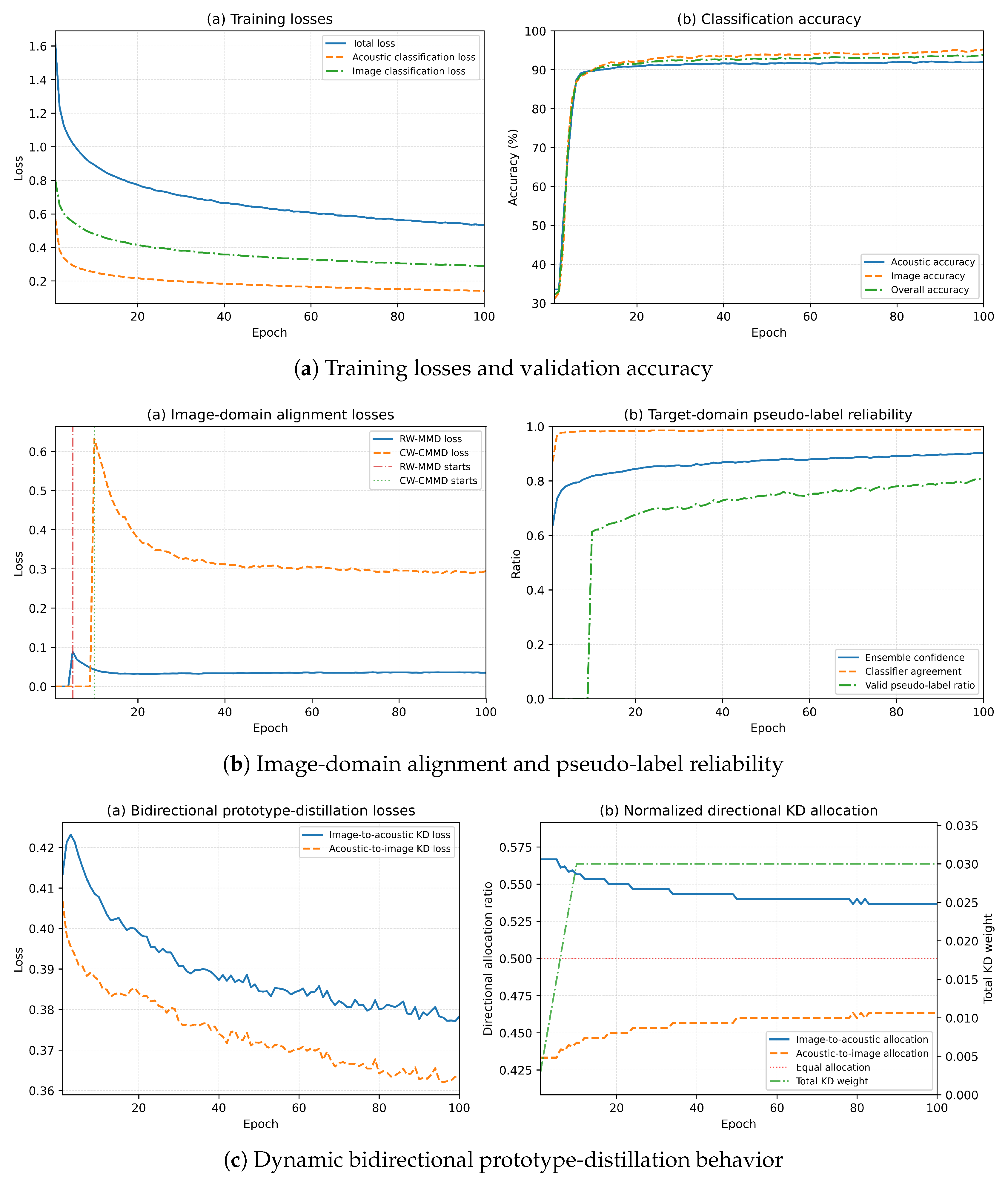
Figure 6 summarizes the optimization process. The total and task-specific classification losses decrease rapidly in the early epochs and then converge. Acoustic, image, and overall validation accuracies increase consistently and then stabilize. The two image-domain alignment losses activate at their scheduled epochs, while ensemble confidence, classifier agreement, and the valid pseudo-label ratio improve as training proceeds.
The total prototype-distillation weight increases to 0.03 during warm-up. The normalized image-to-acoustic allocation decreases from approximately 0.57 to 0.54, whereas the acoustic-to-image allocation increases from approximately 0.43 to 0.46. In addition, the acoustic-to-image distillation loss remains lower overall than the reverse-direction loss. These results show that the two transfer directions differ in difficulty and that the proposed reliability mechanism maintains a stable, moderately asymmetric allocation rather than imposing a fixed 1:1 transfer ratio.
Figure 6.
Training behavior of the proposed framework.
4.3. Comparison with Representative Methods
Nine comparison methods are evaluated. DAN, DANN, CDAN, MCC, MME, and TriCT represent statistical, adversarial, conditional, discriminative, and semi-supervised image-domain adaptation. CROMA, GMC, and XKD represent weak-pair cross-modal meta-alignment, multimodal contrastive learning, and cross-modal knowledge distillation. For methods requiring acoustic–image inputs, same-class samples are dynamically associated at the batch level, without constructing fixed instance pairs.
Table 5 reports the results. The proposed method achieves 92.02% acoustic accuracy, 95.26% target-image accuracy, and 93.79% overall accuracy. Among the compared methods, CDAN obtains the highest acoustic accuracy of 90.53%, TriCT obtains the highest image accuracy of 94.02%, and TriCT also obtains the highest overall accuracy of 91.32%. The proposed method therefore improves these strongest baseline results by 1.49, 1.24, and 2.47 percentage points, respectively.
Domain adaptation methods improve target-image transfer but generally do not exploit acoustic–image semantic complementarity. TriCT produces strong target-image performance but lower acoustic accuracy, indicating an imbalanced benefit across streams. Compared with TriCT, the proposed method improves target-image accuracy by 1.24 percentage points and acoustic accuracy by 3.99 percentage points, demonstrating a more balanced benefit across the two modalities. Cross-modal methods improve knowledge exchange but do not explicitly resolve the web-to-UGS image shift. Integrating both aspects allows the proposed method to improve the two modalities simultaneously.

Table 5.
Classification performance comparison with domain adaptation and cross-modal learning methods. The best results are shown in bold.
Table 5.
Classification performance comparison with domain adaptation and cross-modal learning methods. The best results are shown in bold.
| Method | Acoustic Accuracy (%) | Image Accuracy (%) | Overall Accuracy (%) | Primary Mechanism |
|---|---|---|---|---|
| DAN [7] | 90.40 | 89.45 | 89.88 | MK-MMD domain alignment |
| DANN [8] | 90.35 | 91.39 | 90.92 | Adversarial domain alignment |
| CDAN [9] | 90.53 | 90.16 | 90.33 | Conditional adversarial alignment |
| MCC [19] | 88.98 | 89.60 | 89.32 | Target class-confusion minimization |
| MME [20] | 89.19 | 72.91 | 80.26 | Semi-supervised minimax entropy |
| TriCT [21] | 88.03 | 94.02 | 91.32 | Semi-supervised tri-training |
| CROMA [10] | 90.34 | 90.12 | 90.22 | Weak-pair meta-alignment |
| GMC [11] | 90.05 | 91.00 | 90.57 | Geometric multimodal contrast |
| XKD [12] | 90.37 | 91.08 | 90.76 | Cross-modal distillation and alignment |
| Proposed method | 92.02 | 95.26 | 93.79 | Reliability-aware joint adaptation |
Figure 7 shows the confusion matrices. Pedestrian targets are classified most reliably in both modalities. The remaining errors mainly occur between tracked and wheeled vehicles, whose acoustic spectra can overlap at varying distances and under different operating states and whose low-resolution grayscale appearances can be similar under occlusion or oblique viewpoints.
Figure 8 presents representative correct predictions and typical errors from the acoustic and target-image test sets. The correctly classified samples show that the model can recognize all three categories across varied spectral patterns and visual appearances. The error cases are consistent with the confusion matrices: acoustically similar vehicle signatures are occasionally interchanged, while small, blurred, or structurally ambiguous image targets can be confused with another vehicle category or with pedestrians. These examples illustrate the model’s prediction behavior and the remaining difficulty posed by low-quality field observations.
4.4. Ablation Study
The ablation study progressively adds reliability-weighted marginal alignment, class-wise conditional alignment, prototype distillation, dynamic directional weighting, and BCMD. Table 6 shows that the shared-backbone baseline (S1) obtains 86.79% overall accuracy. RW-MMD (S2) increases the overall accuracy to 88.94%, demonstrating the importance of correcting global image-domain shift. Adding CW-CMMD (S3) yields 90.02%, indicating that class-aware alignment further improves target discrimination.
Fixed symmetric bidirectional prototype distillation (S4) increases overall accuracy to 91.05%, confirming that class prototypes can transfer semantic information without instance pairs. Dynamic reliability-aware weighting (S5) raises overall accuracy to 92.92%, which is 1.87 percentage points higher than fixed symmetric distillation. Finally, BCMD (S6) produces the best overall accuracy of 93.79%.
Table 6.
Ablation study of the proposed components.
| Setting | Added Component | Acoustic Accuracy (%) | Image Accuracy (%) | Overall Accuracy (%) | Interpretation |
|---|---|---|---|---|---|
| S1 | Shared three-stream backbone | 88.02 | 85.78 | 86.79 | Basic shared representation |
| S2 | S1 + RW-MMD | 89.14 | 88.77 | 88.94 | Marginal image-domain alignment |
| S3 | S2 + CW-CMMD | 90.06 | 89.99 | 90.02 | Class-conditional image alignment |
| S4 | S3 + fixed bidirectional PKD | 90.18 | 91.76 | 91.05 | Category-level cross-modal transfer |
| S5 | S4 + dynamic directional weights | 91.65 | 93.97 | 92.92 | Reliability-aware transfer |
| S6 | S5 + BCMD | 92.02 | 95.26 | 93.79 | Complete model |
4.5. Feature and Prototype Analysis
Figure 9 visualizes target-image embeddings using t-distributed stochastic neighbor embedding (t-SNE) [27]. Without domain alignment, source and target samples form visibly separated distributions. RW-MMD reduces the global domain gap but retains local class overlap. Adding CW-CMMD produces more compact target clusters and clearer class boundaries. These observations are consistent with the quantitative improvement from S1 to S3.
Table 7 reports acoustic–image prototype similarity. Without prototype distillation, the mean same-class similarity is high, but the mean different-class similarity remains positive, resulting in a margin of only 0.432. Fixed distillation increases the margin to 0.490. Dynamic bidirectional distillation produces a mean same-class similarity of 0.986 and a mean different-class similarity of , increasing the inter-class semantic margin to 1.479. These results indicate that dynamic weighting not only aligns corresponding categories but also improves separation between non-corresponding prototypes.
4.6. Model Complexity and Deployment
The auxiliary MLP and GCN classifiers, target pseudo-label ensemble, domain-alignment losses, prototype memories, and BCMD are required only during training. At inference, the model contains the shared feature extractor, modality-dependent batch-normalization parameters, and main classifier. Table 8 compares the training and deployment configurations.
The complete training network contains 156.81 K parameters, of which approximately 33.42 K belong to auxiliary classifiers. The deployment network contains 123.40 K parameters and occupies approximately 0.47 MiB in FP32. Training two independent acoustic and image networks with the same basic architecture would require 237.89 K parameters and approximately 0.91 MiB. Shared learning therefore reduces deployment parameters by 48.13%. A single acoustic or image forward pass activates approximately 118.95 K parameters and requires about 0.00924 GMAC. The two class-prototype banks contain only 768 floating-point values, approximately 3 KiB, and are discarded after training.
Table 8.
Training and deployment complexity.
| Configuration | Parameters (K) | FP32 Storage (MiB) | Active Parameters per Sample (K) | Compute per Sample (GMAC) | Notes |
|---|---|---|---|---|---|
| Full training network | 156.81 | – | – | – | Includes auxiliary classifiers |
| Proposed deployment network | 123.40 | 0.47 | 118.95 | 0.00924 | Single shared model for both input types |
| Two separate deployment networks | 237.89 | 0.91 | 118.95 | 0.00924 | Independent acoustic and image models |
5. Discussion
The results support three main observations. First, image-domain adaptation and cross-modal transfer solve different parts of the problem and are complementary. Global and class-conditional alignment reduce the discrepancy between web and UGS images, while prototype distillation transfers acoustic–image category knowledge. Applying only one of these mechanisms leaves either the domain shift or the cross-modal semantic gap insufficiently addressed.
Second, transfer direction should depend on training state. The 1.87-percentage-point improvement of dynamic weighting over fixed symmetric distillation indicates that the acoustic and image streams do not provide equally reliable supervision throughout optimization. Combining classification confidence, prototype availability, and prototype stability offers a compact way to regulate the teacher role without introducing an additional learned weighting network.
Third, the shared backbone provides both statistical and deployment benefits. Sharing convolutional and classifier parameters allows gradients from the three streams to regularize a common semantic representation. Modality-dependent batch normalization preserves low-level statistical differences, and BCMD discourages over-dependence on one labeled stream. The deployment network is approximately half the size of two independent models while permitting acoustic-only or image-only inference.
Several limitations remain. The current study includes three ground-target categories and evaluates a specific UGS collection environment. Generalization to additional categories, sensor types, weather conditions, geographic regions, and more severe target imbalance requires further validation. The target-image branch uses unlabeled data during training, but the acoustic branch is not explicitly adapted across deployment sites. In addition, the class-prototype formulation captures category-level correspondence but does not model fine-grained subcategories or operating-state variation. Future work should investigate open-set targets, incremental prototype updates, site-adaptive acoustic learning, and uncertainty-calibrated pseudo-label selection.
6. Conclusions
This paper presented an asynchronous acoustic–image joint learning method for UGS target classification under non-paired observations and image-domain shift. A shared three-stream backbone learns from labeled acoustic spectra, labeled mixed-source images, and unlabeled target UGS images. Reliability-weighted marginal and class-conditional alignment improve image transfer; dynamic bidirectional prototype distillation establishes category-level acoustic–image knowledge exchange; and BCMD regularizes the shared model without increasing inference cost. The complete method achieves 92.02% acoustic accuracy, 95.26% target-image accuracy, and 93.79% overall accuracy, outperforming representative domain adaptation and cross-modal learning methods. With 123.40 K deployment parameters and 0.47 MiB FP32 storage, the method is suitable for resource-constrained UGS nodes and other asynchronous heterogeneous sensing systems.
Author Contributions
Conceptualization, Y.W. and B.L.; methodology, Y.W. and L.X.; software, Y.W.; validation, Y.W. and J.P.; formal analysis, Y.W.; investigation, Y.W., L.X. and J.P.; resources, B.L.; data curation, Y.W. and L.X.; writing—original draft preparation, Y.W.; writing—review and editing, Y.W., L.X., J.P. and B.L.; visualization, Y.W.; supervision, B.L.; project administration, B.L.; funding acquisition, Y.W. All authors have read and agreed to the published version of the manuscript.
Funding
This research was funded by the Youth Innovation Promotion Association, Chinese Academy of Sciences, grant number E34YCA1001.
Institutional Review Board Statement
Not applicable. This study did not involve experiments with human participants or animals. The web-sourced pedestrian images comprise publicly available data depicting public scenes and involve no interaction or intervention with individuals; therefore, institutional ethical approval was not required.
Informed Consent Statement
Not applicable.
Data Availability Statement
The data supporting the findings of this study, the trained models, and the source code are available from the corresponding author upon reasonable request. The field-collected UGS data are not publicly available because of security and institutional restrictions, and the web images cannot be redistributed because they are subject to third-party copyright.
Acknowledgments
During the preparation of this manuscript, the authors used OpenAI Codex for language editing and formatting assistance. The authors reviewed and edited the output and take full responsibility for the content of this publication.
Conflicts of Interest
The authors declare no conflicts of interest. The funder had no role in the design of the study; in the collection, analyses, or interpretation of data; in the writing of the manuscript; or in the decision to publish the results.
Abbreviations
The following abbreviations are used in this manuscript:
| UGS | Unattended ground sensor |
| MMD | Maximum mean discrepancy |
| RW-MMD | Reliability-weighted marginal maximum mean discrepancy |
| CW-CMMD | Class-wise conditional maximum mean discrepancy |
| PKD | Prototype knowledge distillation |
| DPKD | Dynamic prototype knowledge distillation |
| BCMD | Balanced complementary modality dropout |
| MLP | Multilayer perceptron |
| GCN | Graph convolutional network |
| EMA | Exponential moving average |
| STFT | Short-time Fourier transform |
| GMAC | Giga multiply–accumulate operations |
References
- Bokareva, T.; Hu, W.; Kanhere, S.; Ristic, B.; Gordon, N.; Bessell, T.; Rutten, M.; Jha, S. Wireless sensor networks for battlefield surveillance. In Proceedings of the Land Warfare Conference; 2006; pp. 1–8.
- Sleefe, G.E.; Ladd, M.D.; McDonald, T.S.; et al. Acoustic and seismic modalities for unattended ground sensors. In Unattended Ground Sensor Technologies and Applications; SPIE: Bellingham, WA, USA, 1999; Volume 3713, pp. 2–9. [CrossRef]
- Torralba, A.; Efros, A.A. Unbiased look at dataset bias. In Proceedings of the IEEE Conference on Computer Vision and Pattern Recognition; 2011; pp. 1521–1528.
- Recht, B.; Roelofs, R.; Schmidt, L.; Shankar, V. Do ImageNet classifiers generalize to ImageNet? In Proceedings of the 36th International Conference on Machine Learning; 2019; pp. 5389–5400.
- Koh, P.W.; Sagawa, S.; Marklund, H.; Xie, S.M.; Zhang, M.; Balsubramani, A.; Hu, W.; Yasunaga, M.; Phillips, R.L.; Gao, I.; et al. WILDS: A benchmark of in-the-wild distribution shifts. In Proceedings of the 38th International Conference on Machine Learning; PMLR: Proceedings of Machine Learning Research, 2021; Volume 139, pp. 5637–5664.
- Pan, S.J.; Yang, Q. A survey on transfer learning. IEEE Trans. Knowl. Data Eng. 2010, 22, 1345–1359.
- Long, M.; Cao, Y.; Wang, J.; Jordan, M. Learning transferable features with deep adaptation networks. In Proceedings of the 32nd International Conference on Machine Learning; 2015; pp. 97–105.
- Ganin, Y.; Ustinova, E.; Ajakan, H.; Germain, P.; Larochelle, H.; Laviolette, F.; Marchand, M.; Lempitsky, V. Domain-adversarial training of neural networks. J. Mach. Learn. Res. 2016, 17, 1–35.
- Long, M.; Cao, Z.; Wang, J.; Jordan, M.I. Conditional adversarial domain adaptation. In Advances in Neural Information Processing Systems; Curran Associates, Inc.: Red Hook, NY, USA, 2018; Volume 31, pp. 1640–1650.
- Liang, P.P.; Wu, P.; Ziyin, L.; Morency, L.P.; Salakhutdinov, R. Cross-modal generalization: Learning in low-resource modalities via meta-alignment. In Proceedings of the 29th ACM International Conference on Multimedia, Virtual Event, China, 20–24 October 2021; pp. 2680–2689. [CrossRef]
- Poklukar, P.; Vasco, M.; Yin, H.; Melo, F.S.; Paiva, A. Geometric multimodal contrastive representation learning. arXiv 2022, arXiv:2202.03390.
- Sarkar, P.; Etemad, A. XKD: Cross-modal knowledge distillation with domain alignment for video representation learning. Proc. AAAI Conf. Artif. Intell. 2024, 38, 14875–14885. [CrossRef]
- Hangloo, S.; Arora, B. Multimodal fusion techniques: Review, data representation, information fusion, and application areas. Neurocomputing 2025, 649, 130827. [CrossRef]
- Zhao, F.; Zhang, C.; Geng, B. Deep multimodal data fusion. ACM Comput. Surv. 2024, 56, 1–36. [CrossRef]
- Ngiam, J.; Khosla, A.; Kim, M.; Nam, J.; Lee, H.; Ng, A.Y. Multimodal deep learning. In Proceedings of the 28th International Conference on Machine Learning, Bellevue, WA, USA, 28 June–2 July 2011; pp. 689–696.
- Owens, A.; Wu, J.; McDermott, J.H.; Freeman, W.T.; Torralba, A. Ambient sound provides supervision for visual learning. In Proceedings of the European Conference on Computer Vision, Amsterdam, The Netherlands, 11–14 October 2016; pp. 801–816.
- Arandjelović, R.; Zisserman, A. Look, listen and learn. In Proceedings of the IEEE International Conference on Computer Vision, Venice, Italy, 22–29 October 2017; pp. 609–617.
- Gretton, A.; Borgwardt, K.M.; Rasch, M.J.; Schölkopf, B.; Smola, A. A kernel two-sample test. J. Mach. Learn. Res. 2012, 13, 723–773.
- Jin, Y.; Wang, X.; Long, M.; Wang, J. Minimum class confusion for versatile domain adaptation. In Proceedings of the European Conference on Computer Vision, Glasgow, UK, 23–28 August 2020; pp. 464–480.
- Saito, K.; Kim, D.; Sclaroff, S.; Darrell, T.; Saenko, K. Semi-supervised domain adaptation via minimax entropy. In Proceedings of the IEEE/CVF International Conference on Computer Vision; 2019; pp. 8050–8058.
- Ngo, B.H.; Chae, Y.J.; Kwon, J.E.; Park, J.H.; Cho, S.I. Improved knowledge transfer for semi-supervised domain adaptation via Trico training strategy. In Proceedings of the IEEE/CVF International Conference on Computer Vision; 2023; pp. 19214–19223.
- Zou, Y.; Yu, Z.; Kumar, B.V.K.V.; Wang, J. Unsupervised domain adaptation for semantic segmentation via class-balanced self-training. In Proceedings of the European Conference on Computer Vision, Munich, Germany, 8–14 September 2018; pp. 289–305.
- Gupta, S.; Hoffman, J.; Malik, J. Cross modal distillation for supervision transfer. In Proceedings of the IEEE Conference on Computer Vision and Pattern Recognition, Las Vegas, NV, USA, 27–30 June 2016; pp. 2827–2836.
- Hinton, G.; Vinyals, O.; Dean, J. Distilling the knowledge in a neural network. arXiv 2015, arXiv:1503.02531. [CrossRef]
- Snell, J.; Swersky, K.; Zemel, R.S. Prototypical networks for few-shot learning. In Advances in Neural Information Processing Systems; Curran Associates, Inc.: Red Hook, NY, USA, 2017; Volume 30.
- Wen, Y.; Zhang, K.; Li, Z.; Qiao, Y. A discriminative feature learning approach for deep face recognition. In Proceedings of the European Conference on Computer Vision, Amsterdam, The Netherlands, 11–14 October 2016; pp. 499–515.
- Van der Maaten, L.; Hinton, G. Visualizing data using t-SNE. J. Mach. Learn. Res. 2008, 9, 2579–2605.
- Oppenheim, A.V.; Schafer, R.W. Discrete-Time Signal Processing, 3rd ed.; Pearson: Upper Saddle River, NJ, USA, 2010.
- Chang, W.G.; You, T.; Seo, S.; Kwak, S.; Han, B. Domain-specific batch normalization for unsupervised domain adaptation. In Proceedings of the IEEE/CVF Conference on Computer Vision and Pattern Recognition, Long Beach, CA, USA, 15–20 June 2019; pp. 7354–7362.
- Sandler, M.; Howard, A.; Zhu, M.; Zhmoginov, A.; Chen, L.C. MobileNetV2: Inverted residuals and linear bottlenecks. In Proceedings of the IEEE/CVF Conference on Computer Vision and Pattern Recognition; 2018; pp. 4510–4520. [CrossRef]
- Kipf, T.N.; Welling, M. Semi-supervised classification with graph convolutional networks. In Proceedings of the International Conference on Learning Representations; 2017.
- Neverova, N.; Wolf, C.; Taylor, G.; Nebout, F. ModDrop: Adaptive multi-modal gesture recognition. IEEE Trans. Pattern Anal. Mach. Intell. 2016, 38, 1692–1706.
- Kingma, D.P.; Ba, J. Adam: A method for stochastic optimization. In Proceedings of the International Conference on Learning Representations; 2015.
- Tarvainen, A.; Valpola, H. Mean teachers are better role models: Weight-averaged consistency targets improve semi-supervised deep learning results. In Advances in Neural Information Processing Systems; Curran Associates, Inc.: Red Hook, NY, USA, 2017; Volume 30.
Figure 1.
Representative UGS deployment environments and field-collected target observations. The examples illustrate variations in illumination, background, target distance, and apparent target scale.
Figure 1.
Representative UGS deployment environments and field-collected target observations. The examples illustrate variations in illumination, background, target distance, and apparent target scale.
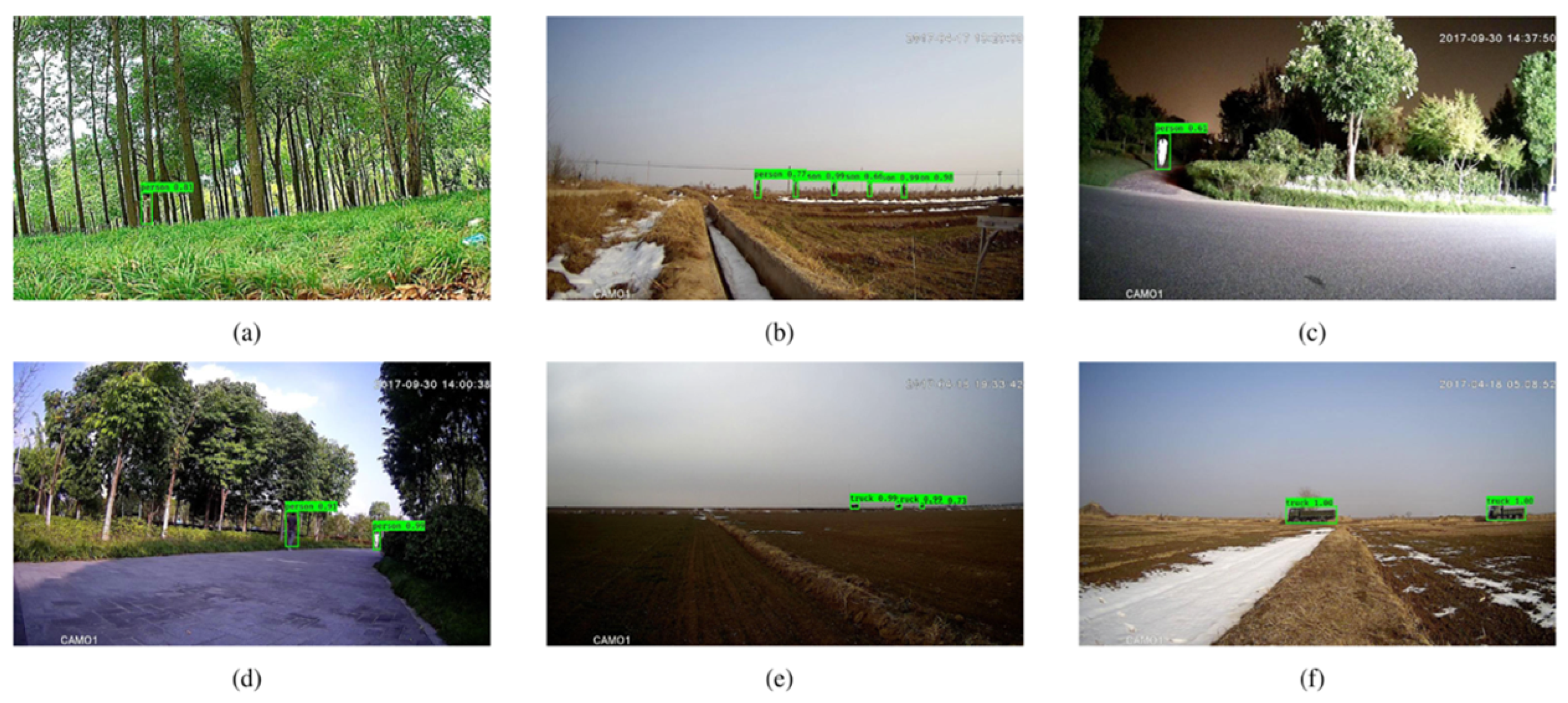
Figure 2.
Examples of the heterogeneous inputs used in this study. The acoustic and image samples share category labels but are not instance-level pairs.
Figure 2.
Examples of the heterogeneous inputs used in this study. The acoustic and image samples share category labels but are not instance-level pairs.
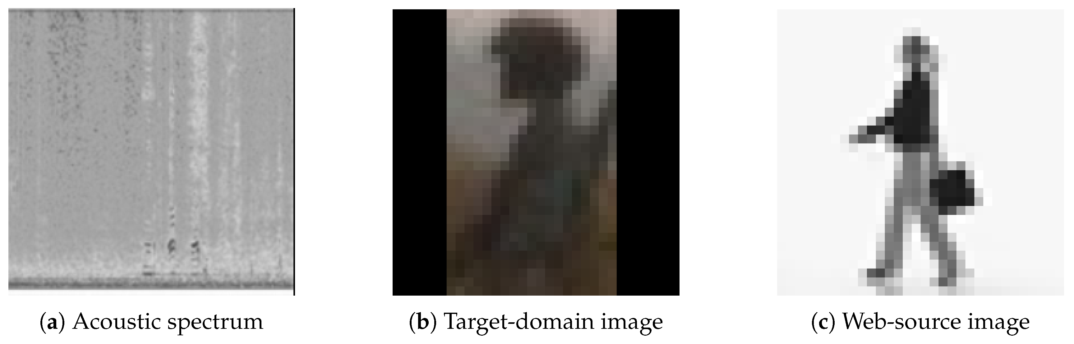
Figure 4.
Reliability-aware dynamic bidirectional prototype distillation. Modality-specific class prototypes provide category-level semantic supervision without requiring synchronized acoustic–image pairs.
Figure 4.
Reliability-aware dynamic bidirectional prototype distillation. Modality-specific class prototypes provide category-level semantic supervision without requiring synchronized acoustic–image pairs.
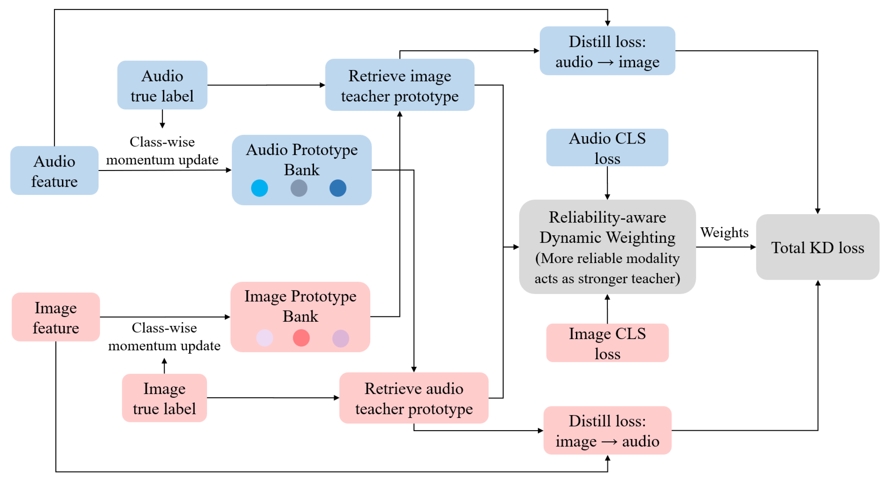
Figure 5.
Balanced complementary modality dropout. The stochastic gate acts only on the residual transformation path, while the identity shortcut remains active.
Figure 5.
Balanced complementary modality dropout. The stochastic gate acts only on the residual transformation path, while the identity shortcut remains active.
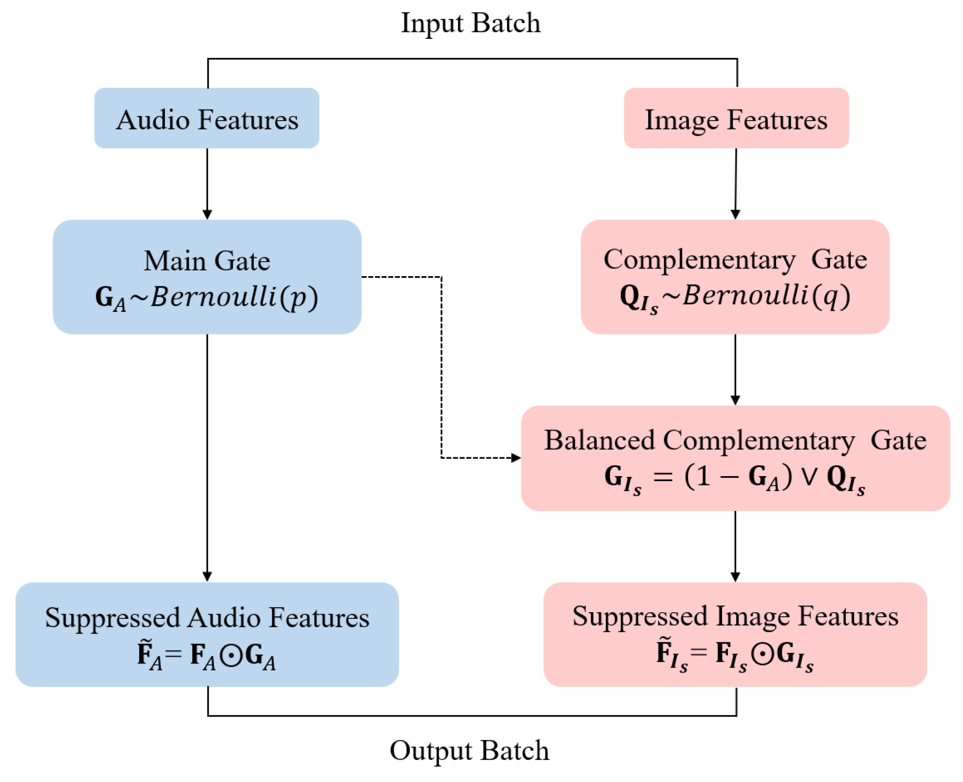
Figure 7.
Confusion matrices of the complete model.
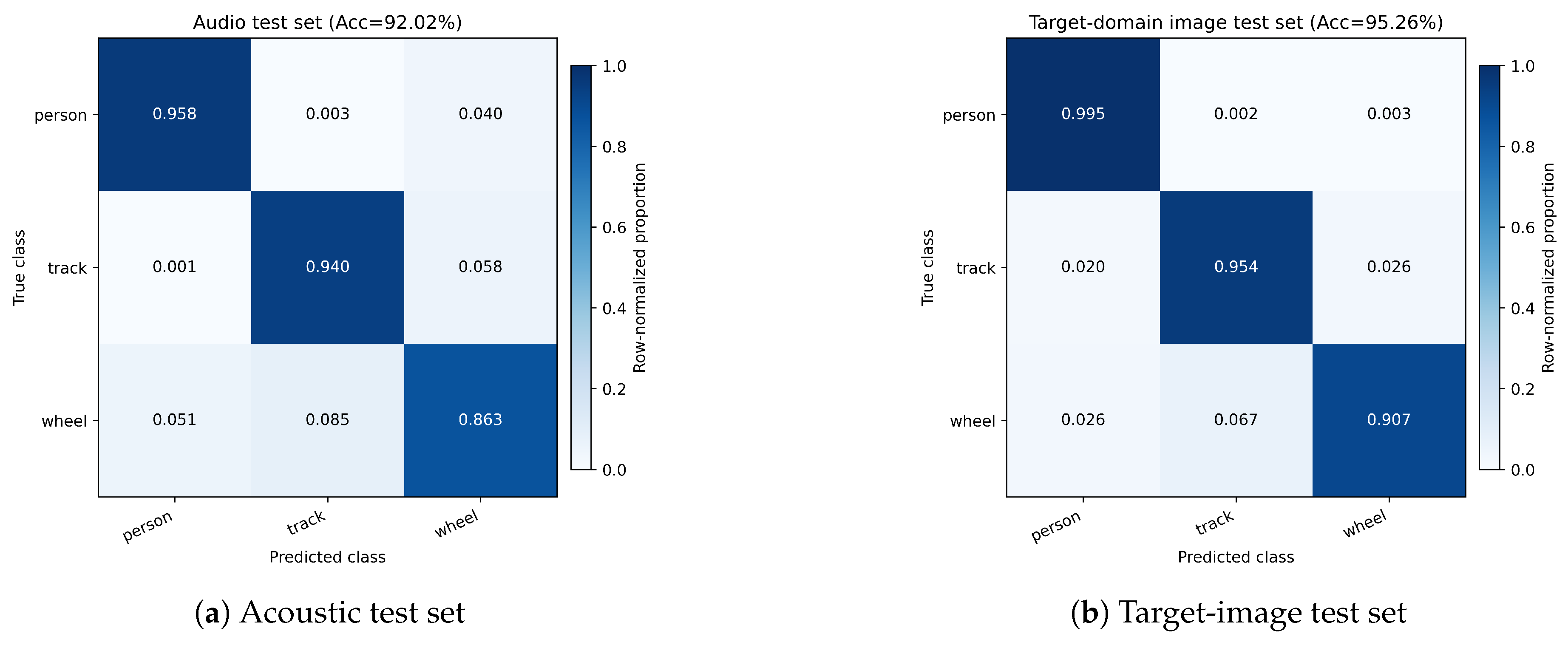
Figure 8.
Representative correct and incorrect predictions on (a) acoustic spectra and (b) target-domain images. Error labels indicate the ground-truth class followed by the predicted class.
Figure 8.
Representative correct and incorrect predictions on (a) acoustic spectra and (b) target-domain images. Error labels indicate the ground-truth class followed by the predicted class.
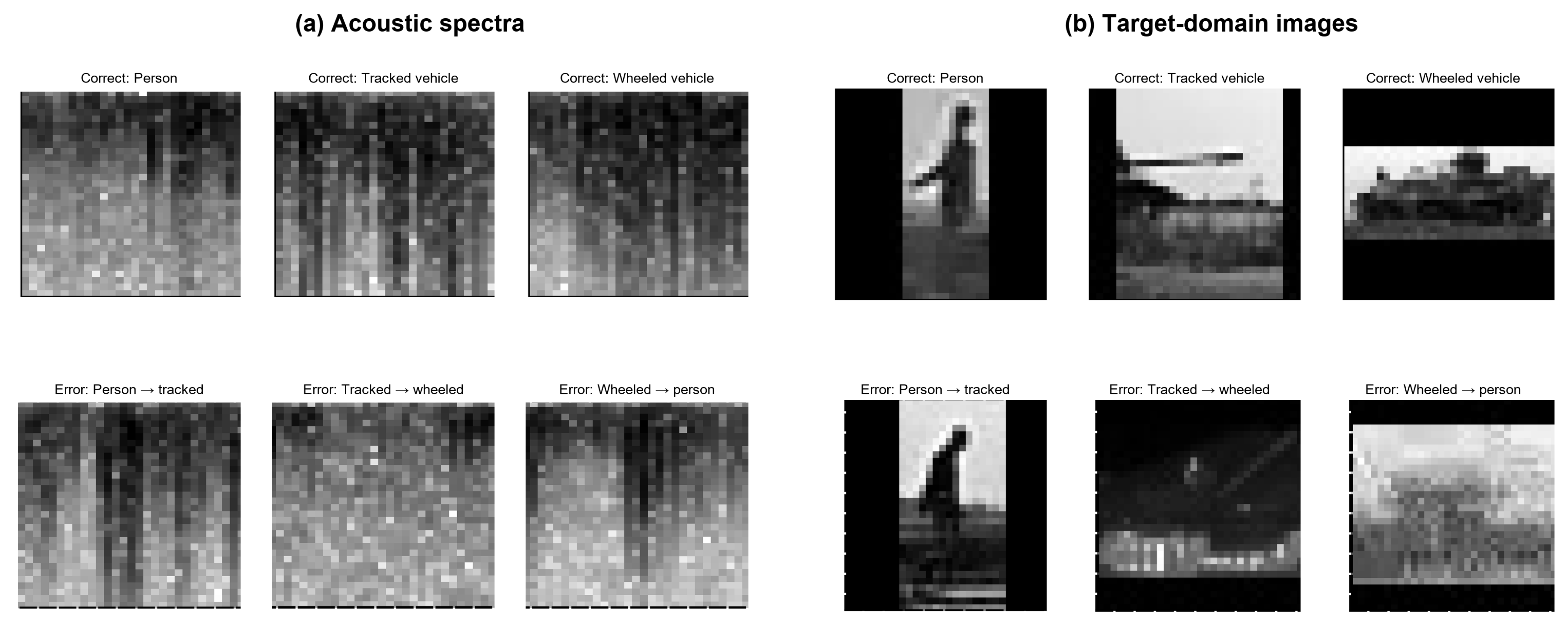
Figure 9.
t-SNE visualization of image features under different domain-alignment configurations.
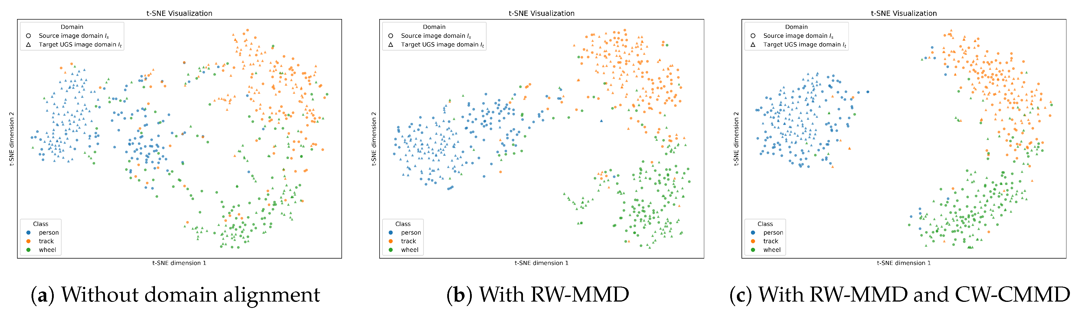
Figure 10.
Acoustic–image class-prototype similarity matrices.
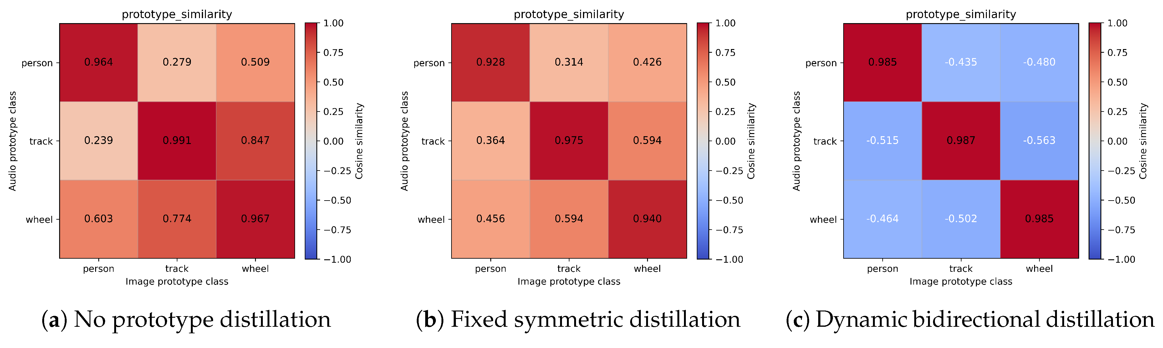
Table 1.
Distribution of the acoustic dataset.
| Class | Training | Validation | Test | Total |
|---|---|---|---|---|
| Pedestrian | 39,261 | 5,106 | 4,762 | 49,129 |
| Tracked vehicle | 39,225 | 4,876 | 5,004 | 49,105 |
| Wheeled vehicle | 39,709 | 5,166 | 4,929 | 49,804 |
| Total | 118,195 | 15,148 | 14,695 | 148,038 |
Table 2.
Distribution of the image dataset. Parentheses in the labeled mixed-source column report web and labeled UGS samples, respectively.
Table 2.
Distribution of the image dataset. Parentheses in the labeled mixed-source column report web and labeled UGS samples, respectively.
| Class | Labeled Mixed-Source | Unlabeled Target | Target Validation | Target Test | Total |
|---|---|---|---|---|---|
| Pedestrian | 40,613 (39,640 + 973) | 2,919 | 6,015 | 5,839 | 55,386 |
| Tracked vehicle | 41,315 (40,240 + 1,075) | 3,225 | 5,929 | 6,452 | 56,921 |
| Wheeled vehicle | 41,095 (40,168 + 927) | 2,781 | 6,008 | 5,563 | 55,447 |
| Total | 123,023 (120,048 + 2,975) | 8,925 | 17,952 | 17,854 | 167,754 |
Table 3.
Configuration of the shared lightweight backbone.
| Stage | Input Channels | Output Channels | Stride | Shortcut | Output Description |
|---|---|---|---|---|---|
| Stem | 1 | 32 | 1 | No | Initial feature map |
| B1 | 32 | 16 | 1 | No | Inverted residual |
| B2 | 16 | 16 | 1 | Yes | Inverted residual |
| B3 | 16 | 24 | 2 | No | Spatial downsampling |
| B4 | 24 | 24 | 1 | Yes | Inverted residual |
| B5 | 24 | 32 | 2 | No | Spatial downsampling |
| B6 | 32 | 32 | 1 | Yes | Inverted residual |
| B7 | 32 | 64 | 2 | No | Spatial downsampling |
| B8 | 64 | 64 | 1 | Yes | Inverted residual |
| B9 | 64 | 96 | 1 | No | High-level representation |
| B10 | 96 | 96 | 1 | Yes | Domain-alignment feature |
| Head | 96 | 128 | – | – | Global pooled embedding |
Table 4.
Principal training and method hyperparameters.
| Item | Value | Item | Value |
|---|---|---|---|
| Optimizer | Adam | Training epochs | 100 |
| Learning rate | Batch size per stream | 128 | |
| Adam coefficients | Weight decay | 0 | |
| Embedding dimension | 128 | Main dropout | 0.5 |
| Prototype momentum | 0.9 | Stability momentum | 0.9 |
| Prototype stability floor | 0.2 | Distillation temperature | 1.0 |
| Maximum PKD weight | 0.03 | PKD warm-up | 10 epochs |
| Maximum RW-MMD weight | 0.03 | RW-MMD activation | Epoch 5 |
| Maximum CW-CMMD weight | 0.005 | CW-CMMD activation | Epoch 10 |
| Pseudo-label threshold | 0.8 | Minimum class samples | 2 |
| BCMD retention probability | 0.7 | EMA decay | 0.999 |
Table 7.
Cross-modal prototype similarity under different distillation strategies.
| Strategy | Same-Class Similarity | Different-Class Similarity | Similarity Margin | Observation |
|---|---|---|---|---|
| No prototype distillation | 0.974 | 0.542 | 0.432 | High cross-class correlation |
| Fixed symmetric distillation | 0.948 | 0.458 | 0.490 | Moderate separation improvement |
| Dynamic bidirectional distillation | 0.986 | 1.479 | Strong alignment and separation |
Disclaimer/Publisher’s Note: The statements, opinions and data contained in all publications are solely those of the individual author(s) and contributor(s) and not of MDPI and/or the editor(s). MDPI and/or the editor(s) disclaim responsibility for any injury to people or property resulting from any ideas, methods, instructions or products referred to in the content. |
© 2026 by the authors. Licensee MDPI, Basel, Switzerland. This article is an open access article distributed under the terms and conditions of the Creative Commons Attribution (CC BY) license (http://creativecommons.org/licenses/by/4.0/).
Copyright: This open access article is published under a Creative Commons CC BY 4.0 license, which permit the free download, distribution, and reuse, provided that the author and preprint are cited in any reuse.