Preprint
Article

This version is not peer-reviewed.

All-Season Retrieval of Precipitable Water Vapor from High-Resolution ECOSTRESS Thermal Infrared Observations via Symbolic Regression

Submitted:

07 August 2026

Posted:

11 August 2026

You are already at the latest version

Abstract

The ECOSTRESS mission provides high resolution thermal infrared observations that support a wide range of applications ranging from evapotranspiration monitoring and drought assessment to Land Surface Temperature (LST) and emissivity retrieval. Accurate estimation of Precipitable Water Vapour (PWV) is critical for these applications because of strong influence of atmospheric water vapour on thermal infrared radiative transfer that influences emissivity retrieval. The current ECOSTRESS processing chain estimates PWV from GEOS5-FP numerical weather prediction data. In this study, we investigate an alternative approach that retrieves PWV directly from ECOSTRESS thermal brightness temperatures using symbolic Regression (PYSR). Using more than 269,000 spatio-temporally matched ECOSTRESS-GNSS observations, we derived a unified all-season analytical formula capable of estimating PWV without relying on external atmospheric profiles or ancillary emissivity. Instead, the proposed model relies only on readily available and temporally stable ancillary variables, namely digital elevation model (DEM) and Normalized Difference Vegetation Index (NDVI) data. The resulting analytical formulation (All-season PySR) derived using PySR symbolic retrieval achieved a Root Mean Square Error (RMSE) of 7.22 mm and an R2 of 0.624 when evaluated against GNSS-derived precipitable water vapor observations. In order to improve the results, season and regime specific PySR formulas were first developed to provide interpretable PWV estimates for various conditions. These formulas form the initial retrieval component of the Climate-Adaptive Ensemble formula. The Climate Adaptive Ensemble (CAE) combines PySR formulas, ECOSTRESS inputs and historical ERA5 water-vapour profiles to perform a global analytical ridge regression. The resulting output achieved an RMSE of 5.35mm and R2 of 0.781 on test GNSS observations. The CAE formula was further validated on external radiosonde dataset and independent GNSS observations to evaluate its robustness. The methodology proposed here will be extremely useful for future satellite missions using thermal sensors such as TRISHNA (Thermal Infra-Red Imaging Satellite for High-resolution Natural resource Assessment) and LSTM (Land Surface Temperature Radiometer) as the methodology could help in retrieving PWV instantaneously for atmospheric correction instead of depending on external products.

Keywords: 
;  ;  ;  ;  ;  ;  

1. Introduction

Atmospheric water vapour is a fundamental part of the climate system influencing radiative transfer, cloud formation, hydrological cycle, and land-atmosphere energy exchange [1]. Precipitable Water Vapour (PWV) defined as the total amount of water vapour contained in a vertical atmospheric column, is therefore an important variable for weather monitoring, climate applications and remote sensing. PWV has a high variability in both spatial and temporal dimensions, therefore proper high spatiotemporal-resolution maps are required [2]. In the Thermal Infrared Region (TIR), atmospheric water vapour affects the radiance measured by satellite sensors with differing transmissivity at different wavelengths and atmospheric conditions. Accurate PWV information is therefore required to reduce uncertainty in atmospheric correction during Land Surface Temperature (LST) and surface emissivity retrieval [3].
Ground-based techniques, including radiosondes, microwave radiometers, and Global Navigation Satellite System (GNSS) observations through radio occultation, provide valuable PWV measurements. In particular GNSS- derived PWV measurements have become a widely used reference for validating other high quality satellite water-vapour products because it provides continuous, observations with high temporal observations from stations distributed throughout the world [4,5]. However, while accurate GNSS stations only provide point data. Satellite remote sensing therefore plays an essential role in retrieving PWV over regional and global scales. Existing satellite PWV products use a combinations of Visible, near-infrared(NIR), TIR and microwave observations, each with different trade-offs like spatial resolution, temporal coverage, cloud sensitivity, weather forecasts and other ancillary atmospheric information [6,7].
Thermal infrared retrieval methods commonly exploit the differential atmospheric absorption measured between neighbouring spectral channels, particularly in the 10-12 µm split-window region. Early studies demonstrated that split-window radiances could be used to estimate PWV under varying weather and climatological conditions [8,9]. In particular, Landsat-based methods have shown that TIR observations from high spatial resolution satellites can provide useful PWV information for atmospheric correction and LST retrieval [10]. Nevertheless, conventional split-window approaches commonly depend on radiative transfer simulations, first-guess atmospheric profiles or empirical parameterisations [7,11,12]. Recent studies have shown that machine-learning methods can improve the retrieval of PWV from thermal observations by modelling nonlinear relations between brightness temperatures, geographical variables, atmospheric conditions, and reference PWV measurements. Random forest, extreme gradient boosting, deep neural networks, ensemble learning, and LightGBM have been applied to thermal observations from Himawari-8 AHI, Landsat 8 TIRS, and MODIS [13,14,15]. These approaches demonstrate that machine learning models can improve PWV retrieval accuracy relative to conventional split-window formulations. However, many machine-learning models operate as black boxes, require multiple sub-models or seasonal switching, or depend on external ancillary variables that may limit interpretability and operational simplicity.
The ECOsystem Spaceborne Thermal Radiometer Experiment on Space Station (ECOSTRESS) provides multispectral TIR observations from the International Space Station at 70 m spatial resolution [16] and is primarily designed for high resolution monitoring of evapotranspiration, Evaporative Stress Index(ESI) etc. Current ECOSTRESS level-2 LST and emissivity workflow, primarily depends on atmospheric correction driven by GEOS5 atmospheric profiles, with an interpolated PWV estimate from GEOS5 included in the Level-2 product [17]. However, this ancillary information is much coarser in spatial and temporal resolution than ECOSTRESS observations and does not capture local atmospheric variability over heterogeneous landscapes. Because ECOSTRESS thermal bands contain spectral information related to atmospheric water-vapour absorption, they offer the potential to estimate PWV directly from brightness temperatures, providing a scene-consistent, high-resolution alternative or complement to coarse ancillary PWV fields that is spatially aligned with ECOSTRESS observations and suitable for high-resolution atmospheric-correction applications [18].
Symbolic regression using PySR based regression provides a suitable alternative to machine learning based black-box models for this objective because it searches for analytical mathematical expressions directly from data rather than fitting to a black-box model. Unlike conventional machine learning techniques, symbolic regression can produce explicit analytical solutions that can be analysed, reproduced and improved without retraining a model. This is particularly important because it allows us to identify the effects of various terms in equations that are contributing to water vapour retrieval.
This study develops an all-season, all climate PWV retrieval approach based on PySR symbolic regression using ECOSTRESS TIR brightness temperature measurements from ECOSTRESS L1C products, DEM and Normalized Difference Vegetation Index (NDVI) information [19]. The proposed method is trained and evaluated using matched ECOSTRESS and GNSS-derived PWV observations. The final retrieval equation does not require a first-guess atmospheric profile or an external surface-emissivity product as input. The objectives of this study are to: (1) derive a single interpretable all-season all-climate PWV equation from ECOSTRESS observations suitable for atmospheric correction; (2) evaluate its performance against independent GNSS PWV measurements; (3) compare the all-season formulation with seasonal and ensemble symbolic-regression alternatives; and (4) analyse systematic retrieval behaviour across low-, moderate-, and high-PWV conditions. The resulting method is intended to provide a computationally simple PWV product mapped on the ECOSTRESS grid for high-resolution land-surface applications that can be studied and iteratively improved if required.

2. Materials and Methods

2.1. ECOSTRESS Data

The ECOSTRESS sensor, mounted on the International Space Station, provides high-spatial and temporal-resolution thermal infrared observations. In this study, ECOSTRESS data were extracted through the NASA APPEEARS platform and collocated with GNSS-derived precipitable water vapor (PWV) observations. The ECO_L1CT_RAD.002 product was used to obtain the five thermal infrared radiance bands, which were converted to brightness temperature. The ECO_L1B_GEO.002 product provided the observation geometry and surface elevation, including view zenith angle, solar zenith angle, and height. Vegetation and surface information were obtained from the ECO_L2T_STARS NDVI product and the ECO_L2_LSTE.002 provides some L2A PWV observations for comparisons.
The ECOSTRESS brightness temperatures from bands B1-B5, together with view geometry, surface elevation, NDVI, NDVI-derived emissivity were used to create thermal band-ratio features and were used as predictors for PWV retrieval. ECOSTRESS overpasses were temporally matched with GNSS PWV measurements within a ±30 min window. Quality control was applied by retaining physically realistic brightness temperatures between 180 and 350 K, PWV values between 0 and 80 mm, and station elevations between 0 and 5 km; cloudy and water pixels were removed when the corresponding quality layers were available. The final matched dataset was separated into summer, winter and tropical subsets and then combined to develop an all-season PWV retrieval model.
Table 1. ECOSTRESS bands and wavelengths.
ECOSTRESS Band Wavelength (nm)
B1 8280
B2 8780
B3 9060
B4 10520
B5 12000
Surface emissivity was estimated from NDVI-derived fractional vegetation cover (FVC) [20]. FVC represents the proportion of a pixel covered by vegetation and was calculated using the scaled-NDVI approach.
F V C = N D V I N D V I s o i l N D V I v e g N D V I s o i l
F V C = N D V I 0.20 0.86 0.20  
e m i s s i v i t y B 4 = 0.94 1 F V C + 0.99 F V C  
e m i s s i v i t y B 5 = 0.96 1 F V C + 0.99 F V C  
Table 2 provides a list of ECOSTRESS point observations that are matched with GNSS stations for regression and evaluation. The summer mid-latitude dataset contains 422,930 observations from 9,635 stations, while the winter dataset comprises 303,876 observations from 9,988 stations. An additional 81,246 tropical observations from 1,657 stations, acquired during 2023–2025, were included to improve the representation of warm and moisture-rich atmospheric conditions. Importantly summer and winter datasets are classified by taking Northern hemisphere seasons and Southern hemisphere seasons into account. For eg. January to April is classified as winter in Northern hemisphere mid latitudes but classified as Summer in Southern hemisphere mid-latitudes. Altogether the datasets provide 808,052 matched observations covering different seasons, geographical regions, surface temperatures, and atmospheric precipitable water vapour conditions, enhancing performance of regression and thereby helping to create a geographically and seasonally robust PWV retrieval model. Each matched record contains ECOSTRESS brightness temperatures for thermal bands B1–B5, surface emissivity, NDVI, viewing zenith angle, acquisition time, station location and elevation, together with the temporally matched GNSS PWV measurement.
Figure 1 displays the seasonal and spatial variability of the matched dataset. Tropical observations exhibit the highest and broadest PWV distribution., whereas winter mid-latitude observations are substantially drier and have low brightness temperatures across all five ECOSTRESS bands. The monthly distribution shows decent temporal coverage spread throughout the year.

2.2. GNSS Data

High- quality GNSS-derived PWV observations are obtained from the Nevada Geodetic Laboratory(NGL) [21]. These observations were used as reference measurements for model development and evaluation. The GNSS data is temporally matched with ECOSTRESS observations at each station location. Each row of data is subjected to quality control to remove corrupted data, cloud pixels, water pixels and outliers [4,22].
The GNSS observations provide estimates of the Zenith Total Delay (ZTD) which is a combination of Zenith Hydrostatic Delay (ZHD) and Zenith Wet Delay (ZWD).
Z W D = Z T D Z H D
PWV was then calculated from ZWD using a temperature-dependent conversion factor:
P W V = Π T m , Z W D
where Π(Tm) is the PWV conversion factor and Tm is the water-vapour-weighted mean atmospheric temperature.
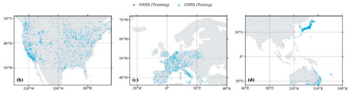
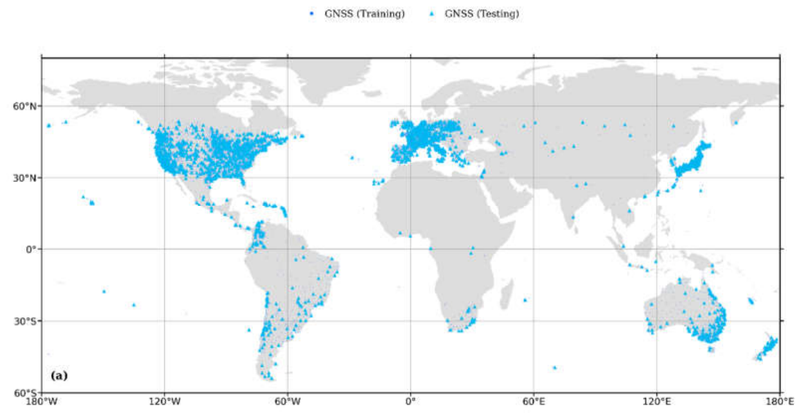
To perform a thorough validation, the matched GNSS stations were separated into training and testing subsets. The geographical distribution of these stations is presented in Figure 2 and Figure 3 with extensive coverage over North America, Europe and Asia, with additional stations distributed across the tropics in Central, south America, Africa, Australia and the Pacific region. To compensate for the reduced GNSS coverage, in the tropical latitudes datasets were taken over multiple years.
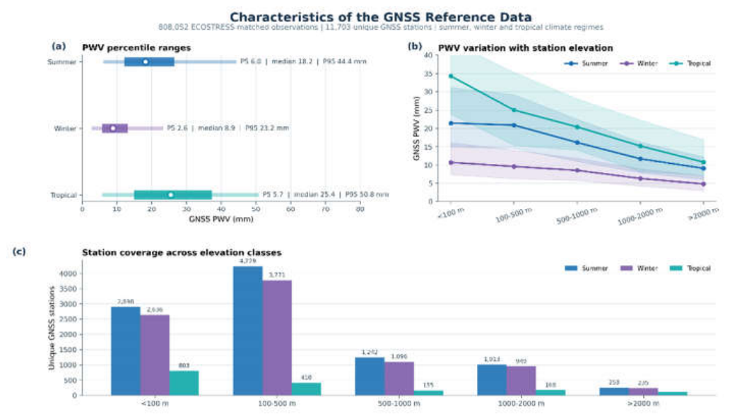
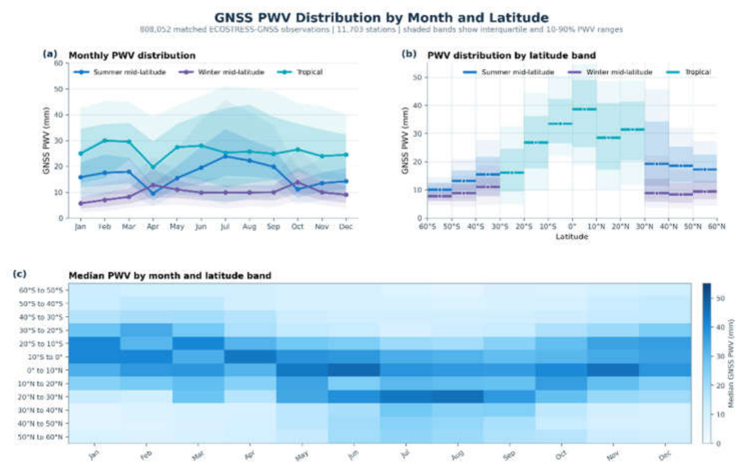
Figure 4 and Figure 5 show the distribution of the reference GNSS data. As expected, the tropical data show the highest median PWV and the largest variability, whereas the winter stations are consistently the driest. PWV decreases systematically with elevation across all regimes. The latitude-month heat map confirms persistent high PWV near the equator and strong seasonal transitions at mid-latitudes.

2.3. PySR Symbolic Regression

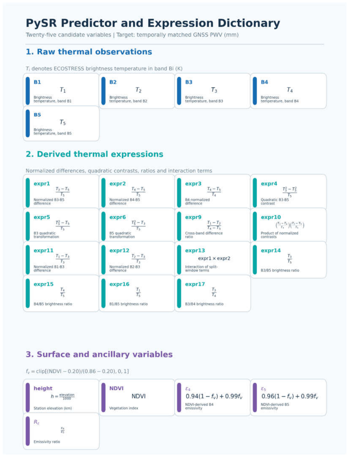
Symbolic regression is a supervised learning task that searches simultaneously for the mathematical structure of a model as well its numerical coefficients. It uses a multi-objective optimization framework to minimize both prediction errors and model complexity. In contrast to conventional regression, where functional equations are specified before fitting, symbolic regression creates candidate analytical equations by combining predictor variables, numerical constants and pre-defined expressions. The pre-defined expressions play the key part in predicting complex expressions with trade-offs in both specificity and complexity. The resulting expressions are evaluated according to both their predictive error (RMSE, R) and algebraic complexity. The list of candidate variables and pre-defined expressions used are shown in the Figure 6.
PySR is an open-source symbolic regression framework developed by Miles Cranmer and built on the SymbolicRegression.jl computational backend [19]. It applies a multi-population evolutionary search to iteratively generate, modify, simplify and optimize best performing equations. In addition to the above mentioned expressions, inputs can also include mathematical operators of choice. Rather than returning only one final candidate equation, PySR identifies a set of equations representing different trade-offs between retrieval accuracy and mathematical complexity. This set, commonly referred to as the Pareto front, enables the selection of a final equation that balances predictive performance with numerical stability, interpretability, and practical applicability.
For our regression the candidate expressions were constructed using the binary operators addition, subtraction, multiplication and division, together with more complex operators like square root, logarithm, absolute value, exponential and square. The search was performed for 1000 iterations using 50 populations, each containing 150 candidate equations. Equation complexity was limited to 50, and a parsimony penalty of 0.0001 was imposed to discourage unnecessarily complicated expressions. Mini-batches of up to 2,000 observations were used during optimization.

3. Methodology

3.1. TIR Based PWV Retrieval Algorithms

The Top Of Atmosphere radiative transfer equation is given by
I λ = ε λ τ λ B λ T s + L λ + τ λ 1 ε λ L λ            
where Iλ is the TOA atmosphere radiance measured by the satellite at wavelength λ, ελ is the surface emissivity at wavelength λ, τλ is the total atmospheric transmittance between the surface and the satellite. B λ T s is the Planck radiance emitted by a blackbody at surface temperature TS. L λ and L λ are the upwelling and downwelling atmospheric path radiance respectively.
The equations rewritten as a function of water vapour shows the effect of water vapour in atmospheric correction:
I λ P W V = ε λ τ λ P W V B λ T s + L λ P W V + τ λ P W V 1 ε λ L λ P W V
Transmittance reduces almost linearly with increase in water vapour. Therefore, variations in precipitable water vapour modify the measured top-of-atmosphere thermal infrared radiance and brightness temperature, providing the physical basis for retrieving PWV from ECOSTRESS thermal bands.
Several previously published TIR-based PWV retrieval methods are based on radiative transfer simulations and creation of regression based relationships between brightness temperature and atmospheric water vapour [11,23]. Operational MODIS thermal-IR water vapour products use multiple infrared channels to estimate water vapour. Split-window techniques have also been widely used for thermal-IR water vapour retrieval. These methods estimate PWV from the differential atmospheric absorption between two thermal bands, commonly around 11 µm and 12 µm. Since water vapour absorption varies between these bands, the brightness temperature difference contains information about atmospheric moisture. Enhanced split-window approaches have further included an additional water vapour absorption band to improve retrieval accuracy, particularly under dry atmospheric conditions. However, split-window methods remain sensitive to measurement noise, surface emissivity uncertainty, cloud effects, and the ability of water vapour to saturate these thermal bands at high humidities [12].
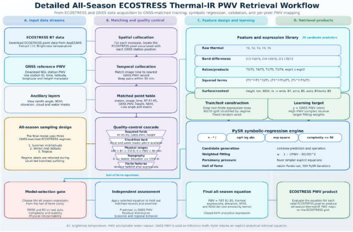
The present study uses ECOSTRESS L1C brightness temperature to develop an empirical approach for retrieving PWV using GNSS-derived PWV as reference. In contrast to MODIS or Aster we lack special water vapour absorption bands to accurately estimate water vapour. So simple regression techniques are not enough. Rather symbolic regression is used to identify an analytical relationship between ECOSTRESS brightness temperatures, thermal-band combinations, surface and geometric variables, and GNSS reference PWV. This allows the final retrieval model to retain the interpretability of an explicit equation while using the information contained across the ECOSTRESS thermal bands and ancillary surface variables. The approach therefore provides a data-driven alternative for estimating PWV from ECOSTRESS observations while reducing reliance on first-guess atmospheric profiles [24]. Figure 7 shows a detailed flowchart of the PWV retrieval process using PySR symbolic regression.

3.2. PySR Based Water Vapour Retrieva

3.2.1. Selection of PySR for Symbolic Regression

The proposed PWV retrieval problem involves non-linear interactions among ECOSTRESS thermal brightness temperatures, atmospheric water vapour, surface conditions like NDVI, NDVI- derived emissivity, view geometry and station elevation. Initially several conventional regression approaches were examined. These include Multiple linear regression, ridge regression, Lasso regression and elastic net regression [25,26]. However, these models were limited in their ability to represent the complex and potentially higher level non-linear relationship between atmospheric water vapour and Brightness temperature.
In addition, more advanced machine-learning models were also evaluated, including convolutional neural network (1-D CNN), random forest regression [27] and Light Gradient Boosting based regression (LightBGM). Many of these complex machine learning models were able to decently capture the complex spectral relationships pertaining to water vapour between the different bands. However, due to the closed nature of machine learning models, it is difficult to interpret the contribution of individual variables or express the relationship in an easier to understand and implement analytical equation.
To obtain an interpretable retrieval formula, symbolic regression was implemented using the PySR framework. Unlike the CNN and Transformer models, the PySR output is an explicit analytical expression that can be inspected term by term and applied directly without retaining the trained model architecture. The resulting equation can therefore be examined to identify the relative role of ECOSTRESS brightness-temperature combinations, NDVI, viewing geometry, and station elevation in the PWV retrieval. This transparency is particularly useful for assessing whether the retrieved relationships are physically plausible and suitable for transfer to additional ECOSTRESS scenes. Table 3 provides a chart of performance of various comparable regression techniques.

3.2.2. Model Definition and Expressions Used

The proposed PWV retrieval model uses all five ECOSTRESS thermal-infrared bands, centred at approximately 8.29, 8.78, 9.20, 10.49, and 12.09 μm. These bands provide complementary information on atmospheric absorption, surface emission, and split-window spectral behaviour.
The model input comprises the 5 Brightness temperatures, 5 derived spectral expressions, station elevation, NDVI, and three NDVI-derived emissivity parameters. The spectral expressions include normalized band differences, band ratios, squared-temperature combinations, and interactions between selected thermal bands. The emissivity parameters consist of the estimated emissivity’s for bands 4 and 5 and their ratio. Together, these variables represent atmospheric absorption, interband thermal behaviour, surface elevation, vegetation conditions, and surface-emissivity variability. Latitude, longitude, month, and other location- or time-dependent predictors are not included, reducing reliance on geographically or seasonally specific empirical relationships. . If each variable and expressions is defined as X1, X2, X3… and so on, then the Pysr retrieval problem can be consequently expressed as
P W V = P y S R X 1 , X 2 , . , X 25                
Table 4 shows the input settings used for PySR regression.

3.2.3. Hall of Fame, Pareto-Front analysis

PySR creates and maintains a Hall of Fame containing the best candidate equations identified throughout the evolutionary optimization process. For each candidate expression, the Hall of Fame stores the analytical expression together with its loss value and algebraic complexity. This archive is used to retain promising equations discovered across multiple populations rather than relying only on the final equation generated by a single population [28].
The Pareto front is then subsequently extracted from the Hall of Fame. An equations is considered as a Pareto front when no alternative expression exists that has a lower prediction error and a lower algebraic complexity. Therefore, each optimal equation represents a different trade-off between retrieval accuracy and equation simplicity. The optimization problem can therefore be expressed as
f m i n L f , C f            
where
L(f) = Prediction loss of equation f
C(f) = Complexity of equation f (size of the symbolic expression trees = no. of variables + No. of fitted coefficients + No. of mathematical operators)
For eg. y= x+2 has a complexity of 3 (1 variable, 1 coefficient and 1 mathematical operator)
For two candidate equations, (fa) and (fb), equation (fa) dominates equation (fb) when
  • it has equal or lower prediction loss and equal or lower complexity.
f a < f b   i f     L f a L f b a n d   C f a C f b          
  • It has at least one inequality strictly smaller.
If these 2 conditions are met and the equation is not dominated by any other candidate then the equation is retained on the Pareto front. These equations represent the best available trade-offs between PWV retrieval accuracy and equation simplicity. The final retrieval equation was selected from this set after validation.

3.2.4. Verification Metrics

The performance of the proposed ECOSTRESS PWV retrieval approach was evaluated by comparing the retrieval PWV values with collocated ground-based GNSS observations. Predictions were generated for held-out observations that were not used to fir the retrieval equation.
Four statistical metrics were used: the coefficient of determination R2, root-mean-square error (RMSE), mean bias (MB), and mean absolute error (MAE). These metrics are defined as
R 2 = 1 i = 1 N ( P W V i D e r P W V i G N S S ) 2 i = 1 N ( P W V i G N S S P W V ¯ i G N S S ) 2        
R M S E = 1 N i = 1 N ( P W V i D e r P W V i G N S S ) 2  
M B = 1 N i = 1 N ( P W V i D e r P W V i G N S S )    
M A E = 1 N i = 1 N P W V i D e r P W V i G N S S                                        
Here, P W V i D e r is the PWV retrieved by applying analytical expressions on the ECOSTRESS observation. P W V i G N S S is the corresponding GNSS reference measurement. P W V ¯ i G N S S is the mean GNSS PWV and N is the total number of collocated observations.

3.3. Regime-Based Assessment of Symbolic PWV Retrieval

3.3.1. Summer PySR PWV Retrieval

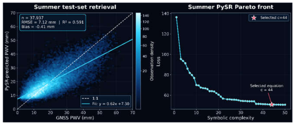
The summer PySR PWV retrieval uses summer-season ECOSTRESS thermal infrared observations matched with references PWV from GNSS data in mid-latitudes. The selected summer PySR expression, with equation complexity 44, was evaluated on 189,690 quality controlled summer ECOSTRESS-GNSS matchups. The reference GNSS PWV ranged from 0.15 to 65.35 mm, with a mean of 20.46 mm. After removing non-physical predictions outside the 0-80 mm range, only 0.0016% of samples were excluded. The retrieval achieved an RMSE of 7.12 mm, MAE of 5.44 mm, bias of -0.41 mm, and R2 of 0.591, indicating moderate predictive skill with a small overall dry bias. Structurally, the formula (Summer PySR) comprises of several split window BT ratios between band 3, 4 and 5. The BT-height gating term |0.171BT3 − 45.852| + height is crucial in treating warm and cold scenes differently. The quadratic height correction (height + 3.184)*(height − 2.861) allows the equation to reduce height dependant bias. Figure 8 shows the results of summer PySR formula on summer test dataset along with Pareto front selection.
Ψ 50 = exp 2.861 h 31.521 T 3 T 5 T 5 68.377 T 3 T 4 T 5 2 0.439 0.151 T 5 2 T 3 T 5 43.762 2 P W V S 50 = N D V I + h + | 0.171 T 4 45.852 | Ψ 50 + T 4 T 5 T 4 [ ( h + 3.184 ) ( h 2.861 ) ] 2 + 7.745

3.3.2. Winter PySR PWV Retrieval

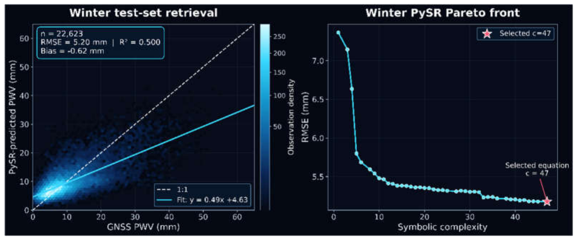
The winter PySR PWV retrieval uses winter-season ECOSTRESS thermal infrared observations matched with references PWV from GNSS data in mid-latitude region. After quality control, the winter dataset contained 113,125 clean samples, with GNSS PWV ranging from approximately 0.0 to 57.8 mm and a mean value of about 10.2 mm, reflecting the dry atmospheric conditions typical of winter scenes. The selected winter analytical expression was the PySR formula with complexity 47. This formula combines emissivity-sensitive terms, elevation correction, split-window brightness temperature ratios, and nonlinear exponential/square root transformations to estimate PWV. Evaluated on the cleaned winter dataset, the c=47 formula achieved an RMSE of approximately 5.18 mm, R2 of 0.495 and a bias of -0.62 mm. Figure 9 shows the results of winter PySR formula on winter test dataset along with Pareto front selection.
Ψ 47 = ε 4 77.309 T 1 T 3 T 3 T 2 T 3 0.055 T 3 + ( T 4 T 5 0.041 T 5 35.709 T 3 T 5 T 5 ) 2 + ( T 4 T 5 0.168 T 5 + 0.237 ) + | T 1 T 3 0.090 T 3 + 0.033 | + 2.100 h + 2.531 + 4.550
P W V W 47 = e x p ( Ψ 47 ) 7.130 + N D V I + T 4 T 5 T 4    

3.3.3. Tropical PySR PWV Retreival

The Tropical PySR PWV retrieval was developed using ECOSTRESS thermal infrared observations matched with tropical GNSS reference PWV measurements. The tropical dataset contains 49,299 clean quality-controlled samples, with GNSS PWV ranging from 0.01 to 77.41 mm, a mean of 24.29 mm, median of 22.58 mm, and a 5th-95th percentile range of 5.16-49.06 mm. Compared with the winter dataset, the tropical subset covers a much wetter and broader PWV regime, so the retrieval must represent stronger atmospheric absorption and a wider range of thermal band ratios.
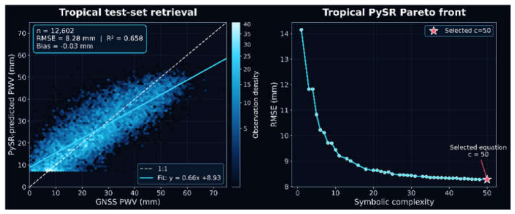
The selected tropical PySR expression has complexity of 50 and produces PWV directly in millimeters. The formula (Equation (18)) combines nonlinear split-window absorption terms, elevation-dependent corrections, emissivity based corrections and high-order band ratio terms to capture the humid tropical atmospheric signal. Evaluated on the cleaned tropical dataset, the c=50 tropical formula produced an RMSE of 8.07 mm, MAE of 6.30 mm, bias of +0.23 mm, and R2 of 0.650, with no predictions removed by the 0-80 mm physical filter. The held-out HOF test performance was similar, with RMSE 8.28 mm and R2 0.658. Overall, the tropical formula shows good results for tropical regions but should not be used for dry winter conditions because of its ability to overestimate PWV in drier conditions.
Φ 50 = h + 0.210 · | T 3 2 T 5 2 T 5 | e x p ( 1.091 h ) T 3 · | T 2 T 3 T 3 · T 3 2 T 5 2 7.199 · T 5 | + 2.423 · T 1 T 3 T 3 · T 5 2 T 3 T 5 | | + 57.400 · T 1 T 3 T 3 7.924 · ε 4 T 3 T 5
I = T 3 T 4 · T 2 T 3 T 3 T 3 T 4
P W V T 50 = ( ε 4 + Φ 50 · I 4 ) 2 + 7.420
The I term can have a significant effect on atmospheric retrieval here. T2−T3 (can be positive or negative): The 8.6 µm vs 9.2 µm slope. Positive when B2 > B3 (very dry), negative when B3 > B2 (moist). Figure 10 shows the results of Tropical PySR formula on tropical test dataset along with Pareto front selection.

3.4. A Generalized All-Season PySR Formula for ECOSTRESS PWV Estimation

A generalized all season and unified formula was developed to provide a single analytical PWV retrieval that can operate across mid-latitude, summer, winter and tropical atmospheric regimes. The advantage of the all-season formula is that it avoids switching between separate seasonal equations. Instead of requiring a user to decide whether a pixel belongs to a summer, winter, or tropical regime, the all-season PySR expression learns a unified relationship from all three datasets. This makes it more practical for large-scale or automated ECOSTRESS processing, especially when scenes contain mixed climates or transitional conditions. In the cross-regime tests, the all-season formula was also more stable than the single-regime formulas, which performed well in their own regime but could become unstable when applied elsewhere.
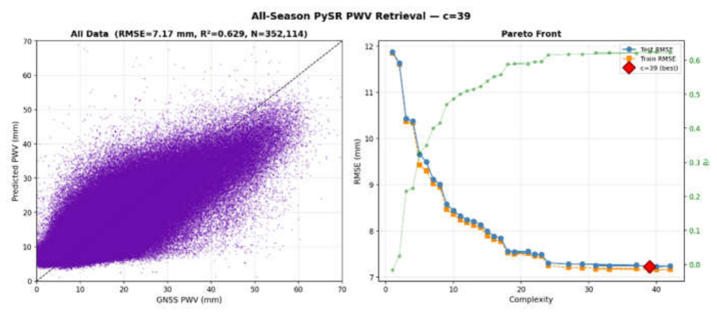
The selected three-regime all-season formula had complexity 39. On the combined all-season evaluation, it achieved approximately 7.17 mm RMSE and R2 = 0.629, with strong stability across summer, winter, and tropical subsets. On individual regimes, the all-season formula gave about 7.38 mm RMSE on summer, 5.71 mm on winter, and 8.88 mm on tropical after anomaly filtering. Although regime-specific formulas can sometimes perform slightly better within their own domain, the all-season formula provides the best balance between accuracy, robustness, interpretability, and operational simplicity.
Indeed, the relative simplicity (c=39) of all-season formula compared to the individual regime formulas make it the best choice for retrieving PWV from ECOSTRESS data.
D = h + 0.675896 · T 3 199.13734 3.706162 2 6.942997 2 + 52.27541 · T 4 T 5 T 4 2 + 1.9237785
S = T 3 2 T 5 2 T 5 + 15.650257 D
P W V A 39 = N D V I + S 2 + 9.6795025 1.2468725 + 0.68907243 · T 3 197.86758 8.442106    
The quadratic band ratio of bands 3 and 5 is the predominant term in overall PWV retrieval.
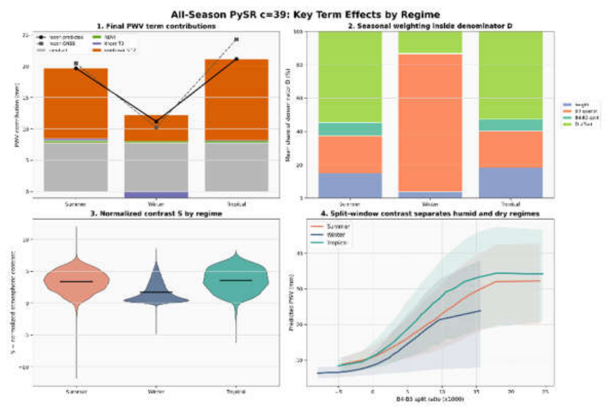
Figure 11 shows the results of all-season PySR formula on overall test dataset along with Pareto front selection. Figure 12 shows the impact of various terms in retrieval of PWV. The B3 quadratic term in particular plays a big role in winter retrieval while the D term (a combination of height factor and split window ratio between band 4 and 5) have outsized contribution in summer and tropical data suggesting higher contribution in humid conditions. In fact, the split window contrast provides a clear difference in predicted PWV across different conditions.

3.5. Climate Adaptive Ensemble (CAE) - Combination of PySR Formulas

Based on the results from the 4 different PySR formulas we developed a more robust algorithm that combines the 4 PySR formulas and assigns various weights based on varying input conditions. In effect CAE follows the general principle of stacked regression with multiple base models supplied to a second-level model to improve model robustness and accuracy [29,30]. The algorithm is also enhanced with the addition of 32 ERA5 based water vapour profiles based on historical water vapour data. A global ridge regression with residual corrections and soft gates are included to further tune the algorithm. This algorithm is trained on the same ~808,000 GNSS-matched ECOSTRESS observations. The algorithm can intelligently choose between the 4 different PySR and assign water vapour profiles weights based on a pre-developed LUT. The key steps are described below,

3.5.1. Stage -PySR Symbolic Experts

4 PySR symbolic experts include the 4 regime based formulas- Mid latitude Summer, Winter, Tropical and All-season.
The four formulas form an N×4 formula matrix:
F = P W V a l l c 39 , P W V s u m m e r c 44 , P W V w i n t e r c 47 , P W V t r o p i c a l c 50
Based on these formulas the derived PySR expert features are computed as based on the following expressions,
f ¯ = 1 4 j = 1 4 f j ( ensemble   mean )  
σ f = max f j min f j i n t e r e x p e r t   s p r e a d  
  s f = 1 3 j = 1 4 ( f j f ¯ ) 2 ( standard   deviation )  

3.5.2. ERA5 Based Water Vapour Profile

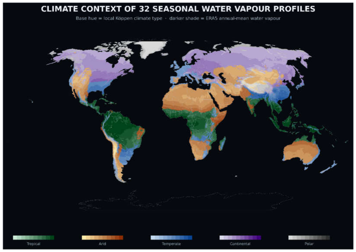
A global ERA5 monthly climatology (2005-2025, 0.25° resolution) profile was developed by using ERA5 total column vapour data for every valid terrestrial grid cell [31]. For each cell, the 12 monthly PWV values were normalized relative to the local annual cycle to obtain an annual shape profile for total column water vapour. This has been performed to make sure that the only contribution of ERA5 climate profiles is to assess the annual seasonal moisture variability rather than providing another absolute PWV estimate. K-means unsupervised classification technique is then used to compress the 807,840 resulting profiles to 32 location based climate profiles with each global grid cell being assigned to its nearest appropriate profile [32]. Basically, the ERA5 data allows us to split the entire globe into 32 distinct climate profiles. Figure 13 shows the map of 32 water vapour profiles created using K-means classification based on the shape of yearly water vapour variability.
The normalization of the 12-month profile to its fractional anomaly shape is given by the equation,
  s h a p e i , m = T C W V i , m T C W V i m a x ( T C W V i , 1.0 )  
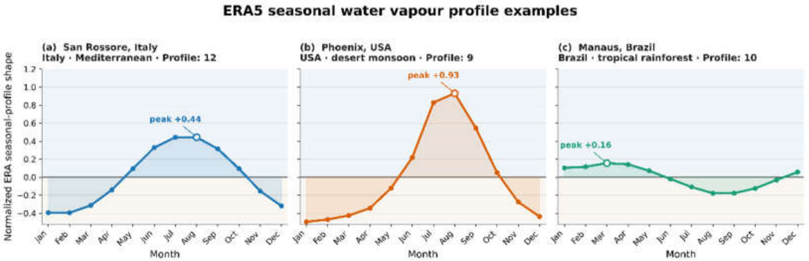
Where T C W V i , m is the total column water vapour at grid cell I in month m and T C W V i is the annual mean. This allows us to remove the absolute magnitude, retaining only the seasonal pattern. Figure 14 shows some examples of normalized seasonal water vapour profile obtained by K-means classification. Note that only the shape of the seasonal profile is retained. The raw water vapour values are not retained as they can have overwhelming influence on the overall retrieval by suppressing contributions from input dataset.

3.5.3. Global Ridge-Regression and Residual Correction

Following the identification and extraction of suitable water vapour profile a global ridge regression model is developed. The global ridge regression is a 70-dimesional feature vector containing base features like ECOSTRESS BT inputs, NDVI, Height, VZA, location, water vapour profile, PySR expert interactions, various feature interactions and expressions defined using BT relations. An ordinary least squares based regression with L2 regularization is performed. The fitted coefficient vector β obtained by ridge-regression is given by,
β ^ = ( X T X + α I ) 1 X T y
Where X is N x 70(training samples * features), y is the GNSS PWV(mm) for each training sample, α=1 is the L2 regularization strength. The final prediction is given by
  y ^ g l o b a l = x n e w . β ^
Where X_new is the 70-dimenstional feature vector for each single ECOSTRESS pixel.
Following this global ridge regression a second stage residual correction is performed after partitioning the input data into 1 of 12 groups. (3 groups based on the 3 PySR regime and 4 PWV bins.) within each group a separate small scale ridge regression is performed. This second stage regression acts as a correctional step for the initial ridge regression in case of anomalous climatic conditions. The residual predictor vector is given by
  x r e s i d u a l = y ^ g l o b a l , f ¯ , σ f , h , N D V I , e x p r 2 , e x p r 3 , e x p r 4 , E R A 5   f r a c t i o n a l   p r o f i l e
For each group g with 2,000 training samples. The residual correction weight is given by.
γ ^ g = ( x r e s , g T x r e s , g + 0.1 I ) 1 x r e s , g T y g y ^ g l o b a l , g  
The raw correction of the second stage residual correction is given by,
  y ^ g = c l i p x r e s . γ ^ g , 6 , + 6
For the 12 groups considered a shrinkage factor Sg is included so that groups with very few stations receive proportionally less importance. Finally, a domain guard weight gate is added to check whether the selected pixel falls predominantly within the training distribution. This allows the model to suppress ridge and residual corrections for anomalous pixel values that don’t fit inside the training distribution. The final derived PWV is given by the equation,
  P W V = y ^ g l o b a l + y ^ g .   s g . w d o m a i n
In practice the entire PWV retrieval can be summed as the PWV retrieved from ridge regression based global regression using PySR inputs plus a small residual correction.

3.5.4. Comparison of Various PySR Formulas and CAE Ensemble

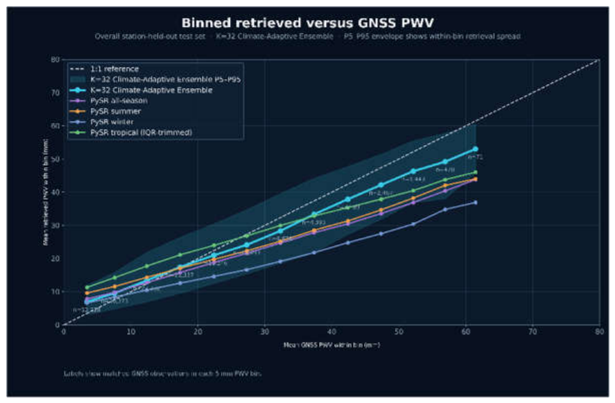
A performance analysis of various PWV formulas is performed against the overall dataset. The CAE ensemble formula, all-season, summer, winter and tropical models are first tested under the same test data. The binned mean predicted PWV curves, as shown in Figure 15, show that all models follow the general increase in GNSS PWV, but none of the equations perfectly follow the 1:1 line at higher water vapour values. The dropoff in predicted PWV at humid conditions can be attributed to various reasons including saturation of thermal bands with respected to PWV, effect of aerosols etc that disturb the band ratios and hence cannot completely capture the full of PWV on thermal bands at very humid as well as very dry conditions. Nevertheless, the performance of CAE ensemble is a clear standout. It scales very well even at high PWV values and only loses some accuracy at extremely high PWV bins.
Out of the 4 base PySR expressions, The all-season c=39 equation provides the most balanced behaviour, with an overall RMSE of 7.13 mm and R2 of 0.633. Its binned curve closely follows the summer and tropical curves through the low-to-moderate PWV range, but begins to underestimate at higher PWV bins. The summer c=44 equation performs similarly to the all-season model, with RMSE = 7.13 mm and R2 = 0.593. Its binned curve is slightly higher than the all-season model at low and mid PWV values. The winter c=47 equation gives the lowest RMSE, 5.18 mm, but its R2 remains moderate at 0.495 because the winter dataset has a narrower and drier PWV range. It generally underpredicts in humid conditions, because the winter formula was optimized for dry/cold atmospheric states and hence not suitable for humid conditions. The tropical c=50 equation shows the highest R2 among the regime-specific models, 0.650, with RMSE = 8.07 mm. It has better PWV retrieval compared to the other 3 formulas in humid conditions but it tends to overestimate PWV in drier conditions.

4. Results and Discussion

4.1. Global Performance

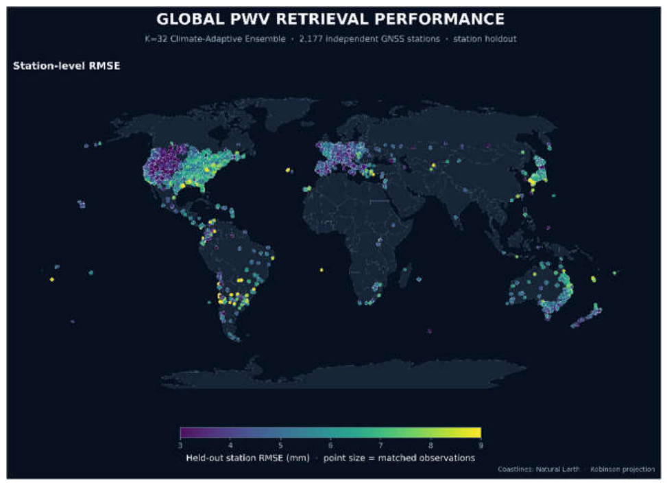
To assess the performance of PWV retrieval and the ability of retrieval to perform across different climates, held-out(test) GNSS stations were assigned to 12 Köppen–Geiger climate regimes using the 1991–2020 climate map [33], and performance was evaluated independently for each regime. As can be seen from Table 5 & Figure 16. The Climate-adaptive ensemble PWV retrieval remained robust across the core PWV retrieval regimes including the main temperate and continental regimes, achieving R2 of 0.798 in temperate-humid climates (Cf; RMSE = 5.78 mm), R2 of 0.743 in continental climates. The weakest results were noted in extremely dry climate regimes including cold-desert (Bwk, R2 =0.408, RMSE=4.63 mm) and polar and Alpine environments (E,ET, R2 =0.265, RMSE=4.91 mm). Part of the reason could be attributed to extreme dry environments, where noise in radiance measurements, aerosol effects could affect water vapour retrieval.

4.2. Climate Adaptive Ensemble Stack Test on San Rossore 2/ICOS Italy(IT-SR2)

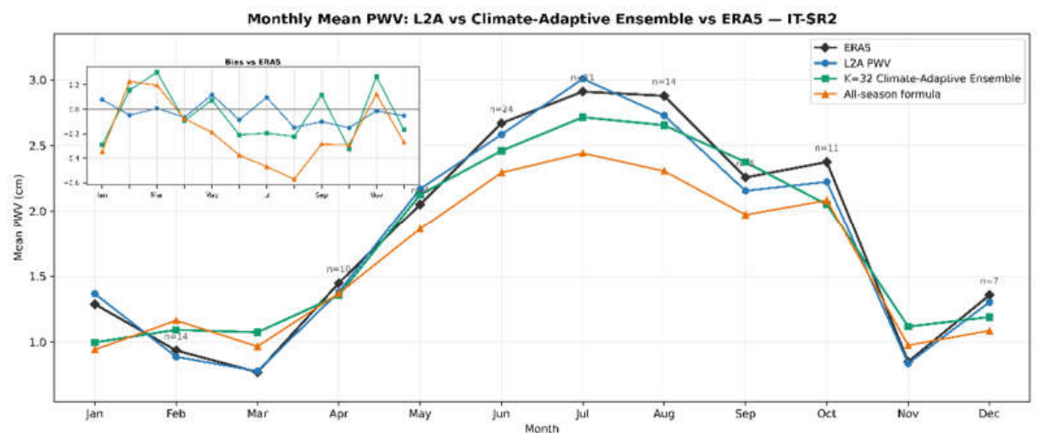
The ensemble stack PWV is tested on ground observations obtained by San Rossore 2 station in Italy. The IT-SR2 station (43.732°N, 10.291°E) is situated within the San Rossore Regional Park in Tuscany, Italy, approximately 5 km west of Pisa at an elevation of 6 m above sea level. The site is characterised by a stone pine / holm oak Mediterranean forest with a broadband emissivity of 0.980. It is part of the ICOS Class 2 / FLUXNET network, providing long-term in-situ measurements of longwave radiation, sensible and latent heat fluxes, and meteorological variables at half-hourly resolution. A total of 309 ECOSTRESS overpasses spanning 2019–2025 were matched with ERA5 hourly TCWV at the nearest grid cell; 105 scenes had valid radiance measurements across all five thermal bands, yielding complete PWV retrievals for comparison. The results from Table 6 & Figure 17 show CAE formula producing good results across an entire year for test performed at San Rossore station.

4.3. PWV Retrieval Performance Against Tropical Radiosonde Dataset

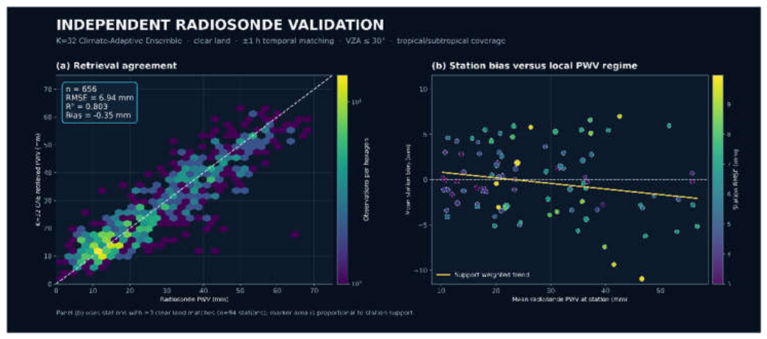
In order evaluate the independent performance of PWV retrieval algorithm the Climate-Adaptive Ensemble PWV retrieval was evaluated against an independent tropical and subtropical radiosonde dataset [34,35,36]. Radiosonde profiles provide vertically resolved temperature and humidity observations, from which column integrated PWV can be derived. ECOSTRESS overpasses were matched to radiosonde observations within ±1 h, with clear-land conditions and view zenith angles ≤30° retained for the primary evaluation. This produced 656 matched retrievals from 172 radiosonde stations. Using the Climate-Adaptive Ensemble, the comparison achieved an RMSE of 6.94 mm, R2 of 0.803, MAE of 5.18 mm, and a small mean bias of −0.35 mm. Results in Figure 18 show that the retrieval retains useful accuracy across humid tropical and subtropical conditions, providing an independent validation of its transferability beyond the GNSS-based development dataset [37]. Therefore, GNSS-derived PWV can be considered to be successfully validated under humid tropical rainforest conditions, supporting its use as a reference across high-moisture atmospheric regimes [38].

4.4. Performance Validation Against ECOSTRESS L2A PWV

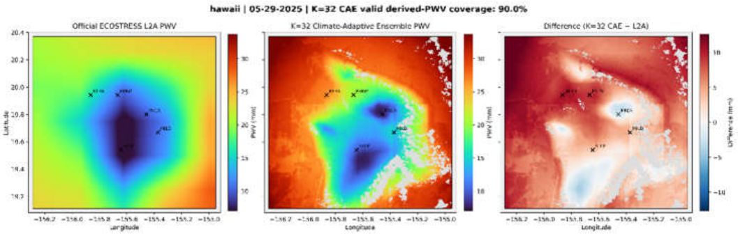
In addition to the independent validation against GNSS-derived PWV, the proposed PySR retrieval PWV was compared with the PWV layer distributed in the ECOSTRESS Level-2 LSTE product. The ECOSTRESS L2 PWV layer is not retrieved directly from ECOSTRESS thermal radiances. Instead, it is derived from GEOS5 atmospheric reanalysis data used in the operational ECOSTRESS atmospheric-correction workflow and is spatially and temporally interpolated to the ECOSTRESS product grid. Unfortunately, PWV from L2A is based on lower resolution products since it is derived from GEOS5-FP atmospheric fields provided at approximately 1/30 longitude by 1/40 latitude every three hours, then spatially and temporally interpolated to the ECOSTRESS acquisition. The 70 m output pixels therefore represent resampled coarse-scale atmospheric information, not independent 70 m PWV observations.
The first case study is Hawaii. It is an interesting example because of its diverse terrain, tropical location and significant elevation changes. Figure 19 shows the results of derived PWV. The CAE retrieval contains substantially finer spatial gradients with variability in PWV expected with increase in elevation. The centre of the island is highly mountainous and shows significant PWV variation.
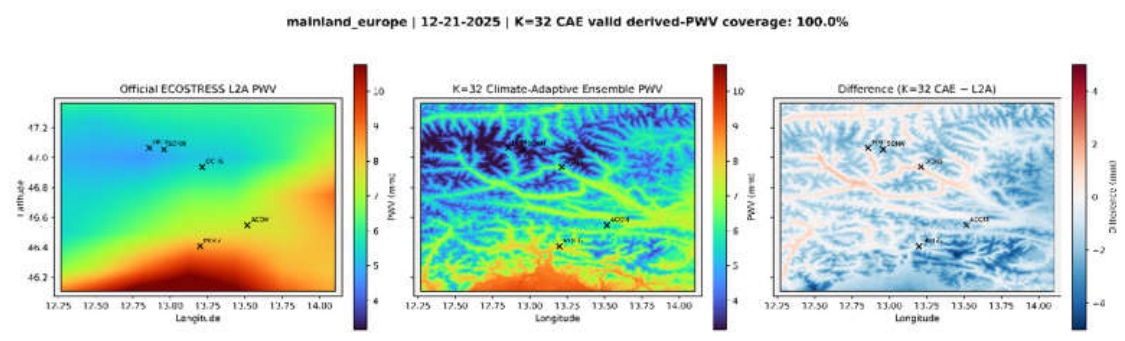
The second case study- Figure 20 is Austrian alps where ensemble PWV is able to identify and isolate pockets of higher PWV in high Alpine valleys. In general, the derived PWV was slightly drier than the official ECOSTRESS L2A PWV.

4.4.1. Emissivity Retrieval Improvements

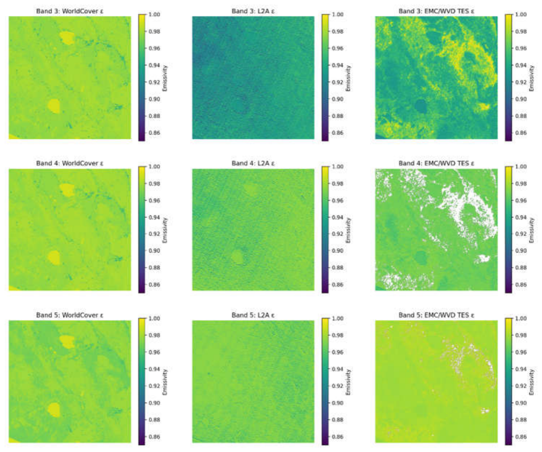
The high-resolution retrieval of PWV allows us to better estimate emissivity using TES [39,40]. The assumption of a scene-wide soft PWV map can induce spatially varying errors into the surface-leaving radiance used by TES. Therefore, PWV at native ECOSTRESS resolution allows us better estimate emissivity pixel by pixel. This is particularly important over heterogeneous terrain and coastal or mountainous environments, where moisture conditions may change substantially within a single coarse atmospheric grid cell.
Figure 21 shows an example of Emissivity retrieved using TES formulation with PWV derived from Climate adaptive ensemble formula. The image is taken on 23/06/205 in central Italy. For comparison we have emissivity derived from Worldcover maps for each band and L2A emissivity provided by ECOSTRESS L2A products [41]. The emissivity derived from TES with the use of our derived PWV is closer to Worldcover reference emissivity than L2A emissivity.

5. Conclusions

This study demonstrates that Precipitable Water Vapour (PWV) can be retrieved directly from multispectral ECOSTRESS thermal-infrared observations using an interpretable analytical framework. 4 PySR symbolic regression formulas were developed for all-season, summer mid-latitude, winter-mid latitude and tropical conditions using ECOSTRESS brightness temperatures together with observation geometry, elevation, NDVI and NDVI-derived emissivity. Finally, an adaptive ensemble technique (CAE) was developed as a stacked ridge regression techniques which combines the four PySR symbolic regression formulas with ECOSTRESS metadata and a compact representation of long-term seasonal moisture behaviour derived from ERA5 historical dataset.
On the held-out GNSS-station benchmark, the CAE reduced the RMSE to 5.35 mm and increased R2 to 0.781, substantially improving upon the stand-alone all-season PySR expression. Performance remained strong in the most densely represented climate regimes, including temperate-humid conditions (R2 = 0.798; RMSE = 5.78 mm) and continental climates (R2 = 0.743; RMSE = 5.45 mm). The climate-stratified assessment also identified the present limits of the retrieval: cold-desert and Polar/Alpine regimes produced R2 values of 0.408 and 0.265, respectively. Nevertheless, RMSE across different regimes was particularly stable (4mm to 6mm) which is comparable to PWV retrieval from other satellites such as MODIS, GOES etc. Independent evaluations support the transferability of the approach with independent testing against Radiosonde dataset achieving an RMSE of 6.94 mm, R2 of 0.803. At San Rossore, 105 complete ECOSTRESS scenes compared with hourly ERA5 TCWV gave an RMSE of 4.42 mm and R2 of 0.738. The scene-based comparisons further illustrate the spatial purpose of the method. The Hawaii and Austrian Alps examples consequently show finer gradients associated with elevation and heterogeneous terrain. The resulting PWV fields also produced physically plausible spatial changes when propagated through the temperature–emissivity separation workflow.
However, several limitations remain. Current challenges include the sparse coverage of GNSS stations in tropical regions. Regions with very low PWV are more difficult to cover using CAE because of increased effects of aerosols, errors due to incorrect surface emissivity assumptions, cloud edges and thin clouds. Overall, the results demonstrate the capability of thermal infrared bands to provide reasonable data for water vapour retrieval used for atmospheric correction and evapotranspiration algorithms. The Climate Adaptive Ensemble is also a fully analytical technique making use of analytical expressions and fitted coefficients to fully retrieve water vapour. Its ability to generate spatially detailed PWV estimates without a contemporaneous first-guess atmospheric profile or auxiliary real time datasets makes it a promising complement to existing ECOSTRESS processing and a transferable framework for future high-resolution thermal missions, including TRISHNA and LSTM.

Data Availability Statement

The ECOSTRESS satellite products used in this study were obtained through NASA’s Application for Extracting and Exploring Analysis Ready Samples (AppEEARS; https://appeears.earthdatacloud.nasa.gov/). The GNSS tropospheric products used to derive PWV are publicly available from the Nevada Geodetic Laboratory (https://geodesy.unr.edu/gps_timeseries/IGS20/trop/). ERA5 reanalysis data are publicly available from the Copernicus Climate Data Store (https://cds.climate.copernicus.eu/datasets/reanalysis-era5-single-levels). Radiosonde observations were obtained from the NOAA National Centers for Environmental Information Integrated Global Radiosonde Archive (IGRA; https://www.ncei.noaa.gov/products/weather-balloon/integrated-global-radiosonde-archive). The processed datasets and code supporting the findings of this study are available from the corresponding author upon request.

Acknowledgments

The authors gratefully acknowledge the financial support of the Italian Space Agency (ASI) under agreement no. 2023-26-HH.0 with INGV for the project “THERESA – THErmal infRarEd SBG Algorithms (CUP F83C23000440005)”.

Conflicts of Interest

The authors declare no conflicts of interest.

References

  1. Sherwood, S.C.; Roca, R.; Weckwerth, T.M.; Andronova, N.G. Tropospheric Water Vapor, Convection, and Climate. Rev. Geophys. 2010, 48, RG2001. [CrossRef]
  2. Allan, R.P.; Willett, K.M.; John, V.O.; Trent, T. Global Changes in Water Vapor 1979–2020. JGR Atmospheres 2022, 127, e2022JD036728. [CrossRef]
  3. Hulley, G.C.; Hughes, C.G.; Hook, S.J. Quantifying Uncertainties in Land Surface Temperature and Emissivity Retrievals from ASTER and MODIS Thermal Infrared Data. J. Geophys. Res. 2012, 117, 2012JD018506. [CrossRef]
  4. Bevis, M.; Businger, S.; Herring, T.A.; Rocken, C.; Anthes, R.A.; Ware, R.H. GPS Meteorology: Remote Sensing of Atmospheric Water Vapor Using the Global Positioning System. J. Geophys. Res. 1992, 97, 15787–15801. [CrossRef]
  5. Vaquero-Martínez, J.; Antón, M. Review on the Role of GNSS Meteorology in Monitoring Water Vapor for Atmospheric Physics. Remote Sensing 2021, 13, 2287. [CrossRef]
  6. Gao, B.; Kaufman, Y.J. Water Vapor Retrievals Using Moderate Resolution Imaging Spectroradiometer (MODIS) Near-infrared Channels. J. Geophys. Res. 2003, 108, 2002JD003023. [CrossRef]
  7. Seemann, S.W.; Li, J.; Menzel, W.P.; Gumley, L.E. Operational Retrieval of Atmospheric Temperature, Moisture, and Ozone from MODIS Infrared Radiances. J. Appl. Meteor. 2003, 42, 1072–1091. [CrossRef]
  8. Kleespies, T.J.; McMillin, L.M. Retrieval of Precipitable Water from Observations in the Split Window over Varying Surface Temperatures. J. Appl. Meteor. 1990, 29, 851–862. [CrossRef]
  9. Ottle, C.; Outalha, S.; FranCois, C.; Le Maguer, S. Estimation of Total Atmospheric Water Vapor Content from Split-Window Radiance Measurements. Remote Sensing of Environment 1997, 61, 410–418. [CrossRef]
  10. Ren, H.; Du, C.; Liu, R.; Qin, Q.; Yan, G.; Li, Z.; Meng, J. Atmospheric Water Vapor Retrieval from Landsat 8 Thermal Infrared Images. JGR Atmospheres 2015, 120, 1723–1738. [CrossRef]
  11. Liu, H.; Tang, S.; Hu, J.; Zhang, S.; Deng, X. An Improved Physical Split-Window Algorithm for Precipitable Water Vapor Retrieval Exploiting the Water Vapor Channel Observations. Remote Sensing of Environment 2017, 194, 366–378. [CrossRef]
  12. Hu, J.; Tang, S.; Liu, H.; Min, M. An Operational Precipitable Water Vapor Retrieval Algorithm for Fengyun-2F/VLSSR Using a Modified Three-Band Physical Split-Window Method. J Meteorol Res 2019, 33, 276–288. [CrossRef]
  13. Lee, Y.; Han, D.; Ahn, M.-H.; Im, J.; Lee, S.J. Retrieval of Total Precipitable Water from Himawari-8 AHI Data: A Comparison of Random Forest, Extreme Gradient Boosting, and Deep Neural Network. Remote Sensing 2019, 11, 1741. [CrossRef]
  14. Wu, Y.; Jiang, N.; Xu, Y.; Yeh, T.-K.; Xu, T.; Wang, Y.; Su, W. Improving the Capability of Water Vapor Retrieval from Landsat 8 Using Ensemble Machine Learning. International Journal of Applied Earth Observation and Geoinformation 2023, 122, 103407. [CrossRef]
  15. Xu, J.; Liu, Z. Machine Learning-Driven Retrieval of All-Weather Precipitable Water Vapor From Satellite MODIS Thermal Infrared Observations. IEEE Trans. Geosci. Remote Sensing 2025, 63, 1–14. [CrossRef]
  16. Fisher, J.B.; Lee, B.; Purdy, A.J.; Halverson, G.H.; Dohlen, M.B.; Cawse-Nicholson, K.; Wang, A.; Anderson, R.G.; Aragon, B.; Arain, M.A.; et al. ECOSTRESS: NASA’s Next Generation Mission to Measure Evapotranspiration From the International Space Station. Water Resources Research 2020, 56, e2019WR026058. [CrossRef]
  17. Hulley, G. ECOsystem Spaceborne Thermal Radiometer Experiment on Space Station (ECOSTRESS) Mission: Level 2 Product User Guide for Collection 3; Jet Propulsion Laboratory, California Institute of Technology;
  18. Dessler, A.E.; Zhang, Z.; Yang, P. Water-vapor Climate Feedback Inferred from Climate Fluctuations, 2003–2008. Geophysical Research Letters 2008, 35, 2008GL035333. [CrossRef]
  19. Cranmer, M. Interpretable Machine Learning for Science with PySR and SymbolicRegression.Jl 2023.
  20. Sobrino, J.A.; Jimenez-Munoz, J.C.; Soria, G.; Romaguera, M.; Guanter, L.; Moreno, J.; Plaza, A.; Martinez, P. Land Surface Emissivity Retrieval From Different VNIR and TIR Sensors. IEEE Trans. Geosci. Remote Sensing 2008, 46, 316–327. [CrossRef]
  21. Blewitt, G.; Hammond, W.; Kreemer, C. Harnessing the GPS Data Explosion for Interdisciplinary Science. Eos 2018, 99. [CrossRef]
  22. Byun, S.H.; Bar-Sever, Y.E. A New Type of Troposphere Zenith Path Delay Product of the International GNSS Service. J Geod 2009, 83, 1–7. [CrossRef]
  23. Knabb, R.D.; Fuelberg, H.E. A Comparison of the First-Guess Dependence of Precipitable Water Estimates from Three Techniques Using GOES Data. J. Appl. Meteor. 1997, 36, 417–427. [CrossRef]
  24. Coll, C.; Caselles, V.; Valor, E.; Niclòs, R. Comparison between Different Sources of Atmospheric Profiles for Land Surface Temperature Retrieval from Single Channel Thermal Infrared Data. Remote Sensing of Environment 2012, 117, 199–210. [CrossRef]
  25. Tibshirani, R. Regression Shrinkage and Selection Via the Lasso. Journal of the Royal Statistical Society Series B: Statistical Methodology 1996, 58, 267–288. [CrossRef]
  26. Zou, H.; Hastie, T. Regularization and Variable Selection Via the Elastic Net. Journal of the Royal Statistical Society Series B: Statistical Methodology 2005, 67, 301–320. [CrossRef]
  27. Breiman, L. Random Forests. Machine Learning 2001, 45, 5–32. [CrossRef]
  28. Bartlett, D.J.; Desmond, H.; Ferreira, P.G. Exhaustive Symbolic Regression. IEEE Trans. Evol. Computat. 2024, 28, 950–964. [CrossRef]
  29. Breiman, L. Stacked Regressions. Mach Learn 1996, 24, 49–64. [CrossRef]
  30. Jacobs, R.A.; Jordan, M.I.; Nowlan, S.J.; Hinton, G.E. Adaptive Mixtures of Local Experts. Neural Computation 1991, 3, 79–87. [CrossRef]
  31. Hersbach, H.; Bell, B.; Berrisford, P.; Hirahara, S.; Horányi, A.; Muñoz-Sabater, J.; Nicolas, J.; Peubey, C.; Radu, R.; Schepers, D.; et al. The ERA5 Global Reanalysis. Quart J Royal Meteoro Soc 2020, 146, 1999–2049. [CrossRef]
  32. Lloyd, S. Least Squares Quantization in PCM. IEEE Trans. Inform. Theory 1982, 28, 129–137. [CrossRef]
  33. Beck, H.E.; McVicar, T.R.; Vergopolan, N.; Berg, A.; Lutsko, N.J.; Dufour, A.; Zeng, Z.; Jiang, X.; Van Dijk, A.I.J.M.; Miralles, D.G. High-Resolution (1 Km) Köppen-Geiger Maps for 1901–2099 Based on Constrained CMIP6 Projections. Sci Data 2023, 10, 724. [CrossRef]
  34. Zhang, Y.; Cai, C.; Chen, B.; Dai, W. Consistency Evaluation of Precipitable Water Vapor Derived From ERA5, ERA-Interim, GNSS, and Radiosondes Over China. Radio Science 2019, 54, 561–571. [CrossRef]
  35. Durre, I.; Yin, X.; Vose, R.S.; Applequist, S.; Arnfield, J.; Korzeniewski, B.; Hundermark, B. Integrated Global Radiosonde Archive (IGRA), Version 2 2016.
  36. Li, Z.; Muller, J.; Cross, P. Comparison of Precipitable Water Vapor Derived from Radiosonde, GPS, and Moderate-Resolution Imaging Spectroradiometer Measurements. J. Geophys. Res. 2003, 108, 2003JD003372. [CrossRef]
  37. Liou, Y.-A.; Teng, Y.-T.; Van Hove, T.; Liljegren, J.C. Comparison of Precipitable Water Observations in the Near Tropics by GPS, Microwave Radiometer, and Radiosondes. J. Appl. Meteor. 2001, 40, 5–15. [CrossRef]
  38. Adams, D.K.; Fernandes, R.M.S.; Maia, J.M.F. GNSS Precipitable Water Vapor from an Amazonian Rain Forest Flux Tower. Journal of Atmospheric and Oceanic Technology 2011, 28, 1192–1198. [CrossRef]
  39. Ru, C.; Duan, S.-B.; Jiang, X.-G.; Li, Z.-L.; Huang, C.; Liu, M. An Extended SW-TES Algorithm for Land Surface Temperature and Emissivity Retrieval from ECOSTRESS Thermal Infrared Data over Urban Areas. Remote Sensing of Environment 2023, 290, 113544. [CrossRef]
  40. Malakar, N.K.; Hulley, G.C. A Water Vapor Scaling Model for Improved Land Surface Temperature and Emissivity Separation of MODIS Thermal Infrared Data. Remote Sensing of Environment 2016, 182, 252–264. [CrossRef]
  41. Hu, T.; Hulley, G.C.; Mallick, K.; Szantoi, Z.; Hook, S. Comparison between the ASTER and ECOSTRESS Global Emissivity Datasets. International Journal of Applied Earth Observation and Geoinformation 2023, 118, 103227. [CrossRef]
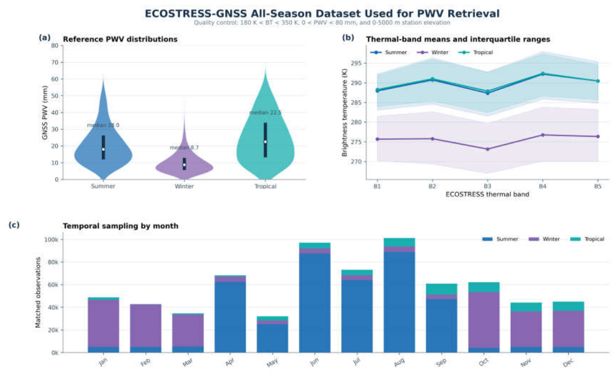
Figure 1. ECOSTRESS-GNSS dataset for PWV retrieval.
Preprints 227368 g001
Figure 2. GNSS stations coverage: North America, Europe and Asia.
Preprints 227368 g002
Figure 3. GNSS stations coverage.
Preprints 227368 g003
Figure 4. GNSS data distribution by station.
Preprints 227368 g004
Figure 5. GNSS data distribution by month and latitude.
Preprints 227368 g005
Figure 6. Input expressions and variables for PySR regression.
Preprints 227368 g006
Figure 7. Detailed workflow for PWV retrieval from ECOSTRESS data using PySR regression.
Preprints 227368 g007
Figure 8. Mid- latitude Summer PWV formula scatter and Pareto Front selection.
Preprints 227368 g008
Figure 9. Mid latitude PySR based PWV retrieval with pareto front selection.
Preprints 227368 g009
Figure 10. Tropical PySR based PWV retrieval with Pareto front selection.
Preprints 227368 g010
Figure 11. Scatter plot comparison of all season PySR PWV vs GNSS PWV and Pareto Front selection.
Preprints 227368 g011
Figure 12. Effect of Different retrieval terms by regime 1. Contribution of T3 , S term, NDVI on PWV retrieval 2. Effect of term D (includes height factor) and band ratio of bands 4 and 5 3. Impact of S term across different regime 4. Split window contrast across humid and dry regimes.
Preprints 227368 g012
Figure 13. ERA5 historical data based global water vapour profile. 32 profiles based on K-means unsupervised classification.
Preprints 227368 g013
Figure 14. ERA5 Seasonal water vapour profile examples.
Preprints 227368 g014
Figure 15. Performance of various PWV formulas vs GNSS reference PWV.
Preprints 227368 g015
Figure 16. Visual representation of test stations with PWV retrieval performance.
Preprints 227368 g016
Figure 17. Monthly PWV mean Climate adaptive Ensemble vs Reference: San Rosssore Year: 2025.
Preprints 227368 g017
Figure 18. PWV Retrieval performance against Radiosonde data a) scatter plot b) station bias plot.
Preprints 227368 g018
Figure 19. Case study Hawaii.
Preprints 227368 g019
Figure 20. Case study: Austrian Alps.
Preprints 227368 g020
Figure 21. WORLDCOVER emissivity VS L2A emissivity VS TES DERIVED emissivity (using PWV from PySR).
Preprints 227368 g021
Table 2. ECOSTRESS point dataset used for the study.
Dataset Rows Stations Date Range
Summer-Mid latitude 422,930 9,635 Jan–Dec 2025
Winter – Mid latitude 303,876 9,988 Jan–Dec 2025
Tropical 81,246 1,657 2023–2025
Table 3. Performance of various comparable regression techniques.
Method RMSE (mm) R2
Climate adaptive Ensemble 5.35 0.781
Deep 1-D CNN 6.42 0.691
Random Forest 6.51 0.683
PySR (c=39) 7.22 0.624
Ridge (α=0.1) 8.03 0.510
Ridge (α=1) 8.03 0.511
Lasso 8.20 0.490
ElasticNet 8.21 0.488
SGD(Linear) 10.77 0.120
Table 4. PySR settings used for PySR symbolic Regression.
PySR setting value
Target variable GNSS PWV(mm)
Binary operators +,-, *, /
Unary operators square root, logarithm, absolute value, exponential, square
Iterations 1000
Number of populations 50
Population size 150
Maximum equation complexity 50
Parsimony coefficient 0.0001
Mini-batch size 2000
Loss function Weighted MSE (mean squared error with sample weights)
Model-selection setting Best test RMSE from hall-of-fame (evaluated on held-out 20% test set)
Random seed 42 (data split + PySR internal)
Table 5. Performance of PWV retrieval across different climate regimes.
Regime N STATIONS Mean PWV RMSE R2
Cold desert (BWk) 5969 78 9.86 4.632 0.408
Cold steppe (BSk) 14437 187 12.86 4.143 0.646
Continental (D) 39904 546 15.62 5.454 0.743
Hot desert (BWh) 4918 75 14.45 5.083 0.673
Hot steppe (BSh) 3907 64 20.20 5.734 0.718
Mediterranean (Cs) 15704 247 15.00 4.828 0.558
Polar/Alpine (E,ET) 721 12 9.08 4.913 0.265
Temperate dry-winter (Cw) 1124 23 17.84 5.344 0.729
Temperate humid (Cf) 44471 803 20.96 5.780 0.798
Tropical monsoon (Am) 545 20 37.85 6.255 0.669
Tropical rainforest (Af) 874 39 33.52 5.777 0.713
Tropical savanna (Aw) 1673 50 32.65 6.066 0.717
Unclassified / ocean 1474 33 20.53 5.947 0.795
Table 6. Climate adaptive ensemble (CAE) performance against reference PWV at San Rossore for 2025.
Model performance vs ERA5 reference R R2 RMSE_cm Bias_cm Mean_PWV_cm
L2A PWV (ECOSTRESS product) 0.977 0.954 0.184 -0.061 2.07
All-season c39 formula 0.705 0.497 0.612 -0.255 1.87
Climate adaptive ensemble PySR 0.875 0.738 0.442 -0.114 2.01
Disclaimer/Publisher’s Note: The statements, opinions and data contained in all publications are solely those of the individual author(s) and contributor(s) and not of MDPI and/or the editor(s). MDPI and/or the editor(s) disclaim responsibility for any injury to people or property resulting from any ideas, methods, instructions or products referred to in the content.
Copyright: This open access article is published under a Creative Commons CC BY 4.0 license, which permit the free download, distribution, and reuse, provided that the author and preprint are cited in any reuse.