
Submitted:
08 August 2026
Posted:
10 August 2026
You are already at the latest version
Abstract
Daily precipitation projections for tropical high-altitude stations are critical for water resource management and flood risk assessment yet remain limited in data-scarce mountain environments. This study applies a chronology-preserving quantile delta mapping framework to five CMIP6 general circulation models under three Shared Socioeconomic Pathways (SSP1-2.6, SSP2-4.5, SSP5-8.5), comparing a historical baseline (1981–2010) with a future period (2051–2080) at a high-altitude tropical station (2160 m a.s.l.) in southern Ecuador. Observations derive from the SC-PREC4SA homogenized daily precipitation product. Pre-correction evaluation across nine performance metrics shows that all raw CMIP6 outputs yield negative Nash-Sutcliffe Efficiency when compared against point-scale observations over complex terrain, consistent with the systematic wet biases intrinsic to coarse-resolution GCM grids. Composite ranking by KGE, NSE, and Pearson r identified MPI-ESM1-2-LR as the best-performing model (r = 0.830). Independent split-sample validation (calibration 1981–2000, evaluation on the withheld 2001–2010 period) confirms genuine out-of-sample skill, with Kling–Gupta efficiency improving from negative values for every raw model to 0.60–0.76 after correction. Ensemble-mean annual precipitation changes are modest and directionally mixed (−1.3% to +5.1%), while extreme-event indices show consistent tail intensification: 50-year daily return levels rise from 67.6 mm day⁻¹ to 76.3–115.2 mm day⁻¹ across models and scenarios. A two-way variance decomposition shows that inter-model structural uncertainty exceeds scenario uncertainty in every calendar month, averaging 75% of total variance against 8% for scenario choice and 17% for their interaction. A Mann–Whitney comparison pooling bootstrap replicates across models detects a statistically significant difference in return levels between SSP2-4.5 and SSP5-8.5, , in contrast with the inconclusive result obtained from the four-to-five point estimates alone, illustrating the sensitivity of such tests to sample construction in small multi-model ensembles. The fully documented computational pipeline constitutes a transferable methodological framework for probabilistic precipitation projection in data-scarce tropical highland stations across the Andes.
Keywords:
statistical downscaling
; CMIP6
; quantile delta mapping
; tropical high-altitude station
; precipitation extremes
; ETCCDI
; Gumbel extreme value
; uncertainty decomposition
; inter-model spread
; SSP scenarios
; independent validation
1. Introduction
Global freshwater availability is increasingly affected by anthropogenic climate change, with precipitation regimes undergoing shifts in intensity, frequency, and seasonality that challenge both engineering design and ecosystem functioning [1,2]. The Andean region of South America hosts some of the world’s most climate-sensitive headwater areas, supplying drinking water and irrigation to millions while simultaneously experiencing accelerating glacier retreat, altered El Niño–Southern Oscillation (ENSO) dynamics, and intensifying extreme rainfall events [3,4]. Across Latin America, hydrological extremes represent among the costliest natural hazards, with documented annual economic losses exceeding USD 20 billion during 2000–2019 according to EM-DAT global disaster records [5], disproportionately affecting mountainous areas where runoff responds non-linearly to precipitation inputs [6]. Understanding how precipitation will evolve under different greenhouse-gas forcing scenarios is therefore a societal imperative with direct implications for infrastructure sizing, flood-risk mapping, and agricultural planning [7].
Southern highland Ecuador occupies a particularly sensitive hydroclimatic niche, straddling the Intertropical Convergence Zone and subject to overlapping atmospheric teleconnections from Pacific and Atlantic sea-surface temperature anomalies [8,9]. The regional precipitation regime emerges from the convergence of South American monsoon outflow, easterly trade-wind moisture advection, and vigorous orographic uplift along an elevation gradient spanning 800–3800 m a.s.l. [10]. The La Argelia meteorological station (3.9999° S, 79.2000° W, 2160 m a.s.l.) provides one of the few continuous daily precipitation records available for the southern Ecuadorian Andes [11]. A single station cannot represent the full spatial variability of precipitation across this elevation gradient, and the projections presented here should accordingly be read as being representative of this specific site rather than of the surrounding region as a whole. Despite the hydrological significance of this location, no published study has simultaneously applied a multi-model CMIP6 ensemble with chronology-preserving statistical downscaling across multiple SSP scenarios at daily resolution using a homogenized observational baseline for this high-altitude station — a methodological gap that constrains science-based water management in southern highland Ecuador.
Statistical downscaling constitutes the principal methodological bridge between coarse-resolution GCM outputs (typically 100–250 km grid cells) and the point-scale observations required for local impact assessment [12,13]. Among available methods, quantile-mapping technique have become the standard approach for daily precipitation because they preserve the full distribution of observed precipitation intensity while correcting systematic GCM biases in both the mean and the tails [14,15]. A distinction of practical importance among quantile-mapping variants is whether the future daily sequence is drawn from the GCM's own projected trajectory or reconstructed from an analogue historical template: the former preserves genuine day-to-day persistence, interannual variability, and any trend embedded in the model's simulated future, while the latter — common in earlier delta-change implementations — can inadvertently substitute the historical record's own temporal structure for the model's projected one. Quantile delta mapping (QDM [16]) addresses this by computing each future day's bias-correction factor from its own rank within the model's future distribution, so that the corrected series inherits its chronology directly from the model's simulated trajectory rather than from a resampled historical analogue.
The Coupled Model Intercomparison Project Phase 6 (CMIP6) ensemble provides unprecedented scenario breadth through the Shared Socioeconomic Pathway (SSP) framework, enabling probabilistic assessments of future precipitation under optimistic (SSP1-2.6), intermediate (SSP2-4.5), and pessimistic (SSP5-8.5) emission trajectories [17]. Multi-model ensemble approaches applied to CMIP6 projections have demonstrated utility in quantifying future precipitation extremes and hydrological flood risk across a wide range of hydroclimatic settings [18,19].
Rigorous GCM performance evaluation prior to downscaling is a methodological prerequisite in applied climate science, as structural biases in raw model outputs directly propagate into projected extreme indices and return-period estimates [20]. The Kling–Gupta Efficiency (KGE [21]) and Nash–Sutcliffe Efficiency (NSE [22]) are widely adopted composite metrics that simultaneously account for correlation, bias, and variability ratio. Taylor diagrams [23] provide complementary visual diagnostics of model skill, enabling identification of structurally diverse model subsets. Independent out-of-sample validation — calibrating a bias-correction transfer function on part of the observational record and evaluating it against a held-out period that never entered calibration — is standard practice for establishing that a statistical downscaling procedure captures genuine predictive skill rather than simply reproducing the data used to fit it [13]. The analysis of ETCCDI extreme precipitation indices—particularly Rx1day, SDII, R95p, CWD, and CDD—is standard in regional climate impact studies because these indices map directly onto engineering design thresholds for drainage infrastructure, agricultural drought, and flood risk [24,25]. Return-period analysis using Gumbel extreme-value distributions, combined with bootstrap confidence intervals, provides decision-relevant probabilistic estimates of peak precipitation for infrastructure design [26]. Partitioning multi-model projection uncertainty into scenario- and model-driven components, following the variance-decomposition logic of Hawkins and Sutton [27], is routine in European and North American regional climate studies but has seen limited application in the tropical Andes, where the relative roles of GCM structural diversity and emission-pathway choice remain poorly quantified for daily precipitation.
To close this gap, this study applies a reproducible multi-model multi-scenario quantile delta mapping framework to five CMIP6 GCMs—ACCESS-CM2, CMCC-ESM2, CanESM5, MIROC6, and MPI-ESM1-2-LR—under SSP1-2.6, SSP2-4.5, and SSP5-8.5 for 2051–2080, calibrated against the SC-PREC4SA homogenized observational record over 1981–2010. The primary contributions are: (i) a chronology-preserving multi-model daily precipitation projection across three SSP scenarios for a high-altitude station in this climatically critical region; (ii) independent split-sample validation demonstrating genuine out-of-sample bias-correction skill; (iii) a comprehensive ETCCDI extreme-index assessment with inter-model confidence envelopes; (iv) Gumbel-fitted return-period estimates with bootstrap 95% confidence intervals suitable for infrastructure design; (v) a two-way variance decomposition quantifying the relative contributions of GCM structure, scenario choice, and their interaction; and (vi) a fully documented computational pipeline, described at algorithmic level in Appendix A, transferable to other high-altitude tropical stations across the Andes.
2. Materials and Methods
2.1. Study Area and Observational Data
La Argelia meteorological station (INAMHI code M0033; 3.9999° S, 79.2000° W; 2160 m a.s.l.) is located on the eastern slope of the Andes in Loja Province, southern Ecuador, within the Northern Andes and Sierra (NAS) ecoregion [28]. The station’s precipitation regime is bimodal, with primary maxima in March–April and a secondary wet period in October–November, driven by the seasonal migration of the ITCZ and easterly trade-wind incursions [10,11]. Daily precipitation observations were sourced from the SC-PREC4SA dataset (Huerta et al. [29]), which provides homogenized and bias-corrected daily precipitation series for 1981–2010 across the NAS ecoregion. The SC-PREC4SA product applies quality control, gap-filling, and homogenization following World Meteorological Organization protocols.
For station M0033, the 1981–2010 reference series comprises 10,957 daily values with 0.00% missing data, a mean of 2.554 mm day⁻¹ (standard deviation 5.418 mm day⁻¹), a maximum of 59.7 mm day⁻¹, 36.8% wet-day frequency (threshold: >1 mm day⁻¹), and a mean annual precipitation of 933 mm year⁻¹, consistent with published climatologies for southern Ecuador [8,11].
2.2. CMIP6 Model Ensemble
Five CMIP6 GCMs were selected based on established performance over the tropical Andes, structural independence, and availability of daily precipitation (variable pr) in the Pangeo CMIP6 cloud catalog: MPI-ESM1-2-LR (Max Planck Institute, Germany); T63 spectral resolution, ~200 km), CMCC-ESM2 (Euro-Mediterranean Centre, Italy; ~100 km), MIROC6 (Japan; ~250 km), CanESM5 (Canada; ~500 km), and ACCESS-CM2 (CSIRO, Australia; ~250 km). This set spans distinct modeling centers, dynamical cores, and convective parameterization schemes, providing structural diversity for the ensemble beyond a single institutional lineage. All models use realization r1i1p1f1. Historical data cover 1981–2010; future data cover 2051–2080 under ssp126, ssp245, and ssp585. A sixth candidate model, NorESM2-LR, was evaluated but excluded because its daily precipitation output was unavailable in the Pangeo catalog for this station and period at the time of analysis. ACCESS-CM2 future data were additionally unavailable for SSP1-2.6 and SSP5-8.5; the effective ensemble size is therefore n = 4 for those two scenarios and n = 5 for SSP2-4.5.
Global GCM output was downscaled directly from the Pangeo CMIP6 catalog rather than from a dynamically downscaled regional product such as CORDEX-CORE, for two reasons specific to this application. First, at the time of analysis the CORDEX-CORE South America domain did not provide a continuous daily precipitation archive at 25 km covering both the historical and all three SSP branches evaluated here for this specific grid cell. Second, the analysis is designed to quantify inter-model structural uncertainty across independent modeling centers (Section 2.8), which requires the broadest available multi-model CMIP6 ensemble rather than the smaller set of driving GCMs typically downscaled by any single regional climate model initiative. Extending this comparison to include CORDEX-CORE simulations as they become available for this domain is identified as a priority for future work (Section 4.5).
2.3. GCM Performance Evaluation
Nine performance metrics were computed by comparing monthly aggregated historical GCM precipitation against the SC-PREC4SA observational record at station M0033 over the 1981–2010 reference period. Negative NSE and sub-optimal KGE values in raw CMIP6 outputs evaluated against point-scale observations over complex terrain are a well-documented consequence of systematic coarse-resolution wet biases, not a reflection of methodological deficiencies [20,30]; composite ranking was therefore based on relative temporal correlation and bias magnitude rather than absolute efficiency thresholds. The metrics are: Pearson r; relative bias; RMSE; MAE; NSE [22]; KGE [21]; PBIAS; wet-day frequency error (WF_err); and the 95th-percentile ratio (P95_ratio [31]). GCMs were ranked by the sum of KGE, NSE, and r ranks (ascending). See Equations (1)-(3).
where α = σₛ/σₒ , β = μₛ/μₒ; Oₘ and Sₘ denote observed and simulated monthly precipitation.
2.4. Quantile Perturbation Downscaling
Before applying the bias-correction procedure to project future precipitation, its out-of-sample skill was tested independently of the future projections themselves. For each model, the transfer function described in Section 2.5 was calibrated using only the 1981–2000 sub-period of the historical record and observations and then applied to the model's own 2001–2010 historical data — a period that never entered calibration — to produce a corrected estimate that could be compared against the observed record for the same withheld years. NSE, KGE, and percent bias were computed for the raw and bias-corrected series in the validation period alike.
2.5. Quantile Delta Mapping Downscaling
Daily precipitation was downscaled using quantile delta mapping (QDM [16]), which corrects each future daily value using a bias-correction factor derived from its own quantile position within the future model distribution, so that the resulting series preserves the day-to-day sequencing, autocorrelation, and any embedded trend of the model's own projected trajectory. For each calendar month m and each model–scenario combination, empirical quantile functions were estimated at 1001 points q ∈ [0, 1] from the historical model series (Qhist), the observed series (Qobs), and the future model series (Qfut). For each future day with value x, the quantile rank τ is its own empirical percentile within Qfut for that calendar month; the historical-model and observed magnitudes at that same rank, Qhist(τ) and Qobs(τ), give the relative perturbation factor RF(τ) = x / [Qhist(τ) + ε] (ε = 10⁻⁶, clipped to the range [0.1, 3.0] to bound the correction near the dry/wet transition, where near-zero historical quantiles would otherwise produce unbounded scaling factors) and the absolute perturbation AF(τ) = x − Qhist(τ). The downscaled value is given by Equation (4).
where FR(τ) and FA(τ) are blended relative and absolute perturbation factors. Blending follows a linear transition between a threshold T_low = 1.0 mm day⁻¹ and T_high = 5.0 mm day⁻¹: below T_low, the absolute factor dominates (preserving near-zero values); above T_high, the relative factor dominates (preserving intensity scaling); in the transition band, a linear weight w = (Q_obs(τ) − T_low)/(T_high − T_low) is applied. The result is indexed by the future day's own real calendar date, so the temporal order of the downscaled series reflects the model's simulated future trajectory rather than a resampled historical sequence. A fixed random seed (numpy seed = 42) was used throughout. All downscaled series cover 2051-01-01 to 2080-12-31 (10,958 daily values per model–scenario combination).
2.6. Extreme Climate Indices (ETCCDI)
Six ETCCDI indices were computed: Rx1day, Rx5day, SDII, R95p, CWD, and CDD, following standard definitions [24,25] (Table 1). All indices were computed per year and averaged over the 30-year analysis window before cross-scenario comparison. In addition to the annual-maximum consecutive wet/dry day counts (CWD, CDD) defined by the ETCCDI framework, the mean and 90th-percentile duration of individual wet and dry spells (threshold 1 mm day⁻¹) were computed across the full record to characterize the typical, rather than the annual-extreme, persistence of precipitation and dry periods.
2.7. Return-Period Analysis
Annual daily maxima were fitted to the Gumbel (Type I GEV) distribution by maximum likelihood, with annual maxima capped at their 99th percentile to limit the leverage of a single extreme outlier year on the fitted parameters; a sensitivity check comparing capped and uncapped fits across all model–scenario combinations showed a mean difference of +0.6% in the 100-year return level, indicating the cap has negligible practical effect at this station. Return quantiles Q(T) were estimated for T ∈ {2, 5, 10, 20, 50, 100} years. See Equation 11.
where μ and β are the Gumbel location and scale parameters. The Gumbel (Type I) distribution was adopted rather than a three-parameter alternative such as the (log-) Pearson Type III or the generalized extreme value (GEV) distribution because the historical annual-maxima series available for direct fitting spans only 30 years; with this sample size, the additional shape parameter of a three-parameter distribution is estimated with substantially greater uncertainty than the two Gumbel parameters, and the two-parameter Gumbel model remains standard practice for daily precipitation extremes of this record length [26]. This choice is revisited in Section 4.4 as a limitation, since tropical precipitation extremes do not always conform to a Type I (light-tailed) shape. Bootstrap 95% confidence intervals (500 resamples with replacement, fixed seed) were derived for each model. Differences in return levels between the SSP2-4.5 and SSP5-8.5 ensembles were assessed with the two-sided Mann–Whitney U test at α = 0.05, computed two ways: first directly on the four-to-five point estimates (one per model), and second on the pooled bootstrap replicates of every model within a scenario (~2000 samples per scenario), which is markedly more informative given the small number of independent model realizations available for the first approach.
2.8. Uncertainty Decomposition
Total projection variance was partitioned into scenario, model, and model × scenario interaction components using a two-way analysis-of-variance sum-of-squares decomposition. For each calendar month m, the total sum of squares of the full scenario × model table of mean monthly values was computed around the grand mean and split into the between-scenario sum of squares, the between-model sum of squares, and the remainder attributed to their interaction. With one realization per scenario–model cell, the interaction term is confounded with any single-realization noise, so no independent residual/error term is separately estimable; this decomposition therefore reports scenario, model, and interaction contributions rather than a fourth, purely random component, and the interaction term should not be interpreted as an estimate of internal climate variability in the sense of Hawkins and Sutton [27], which requires long continuous simulations to isolate.
2.9. Signal-to-Noise Ratio and Model Consensus
The signal-to-noise (S/N) ratio was computed for each calendar month and scenario as |ensemble mean change| divided by the inter-model standard deviation. S/N > 1 indicates that the forced signal exceeds inter-model spread. Model consensus on the sign of change was defined as the fraction of models agreeing on the direction of change (positive or negative), with a robustness threshold of ≥80% adopted in place of a fixed fraction, given that the actual ensemble size varies between four and five models across scenarios (Section 2.2) rather than the six-model design against which a fixed 5-of-6 (83%) criterion would be calibrated.
2.10. Statistical Software and Reproducibility
All analyses were implemented in Python (pandas, numpy, scipy, matplotlib, intake-esm). CMIP6 data were accessed via the Pangeo CMIP6 catalog through Zarr streaming. The random seed was fixed at 42 for all stochastic operations. An algorithmic summary of the computational pipeline is provided in Appendix A.
3. Results
3.1. Observational Baseline and GCM Performance Evaluation
The SC-PREC4SA series (M0033, 1981–2010; N = 10,957; 0.0% missing) exhibits a mean daily intensity of 2.5540 mm day⁻¹ (σ = 5.4180 mm day⁻¹), a wet-day frequency of 36.8%, and a bimodal annual cycle with primary maximum in March (~150 mm) and a secondary wet period spanning October–December (~70–90 mm). See Figure 1.
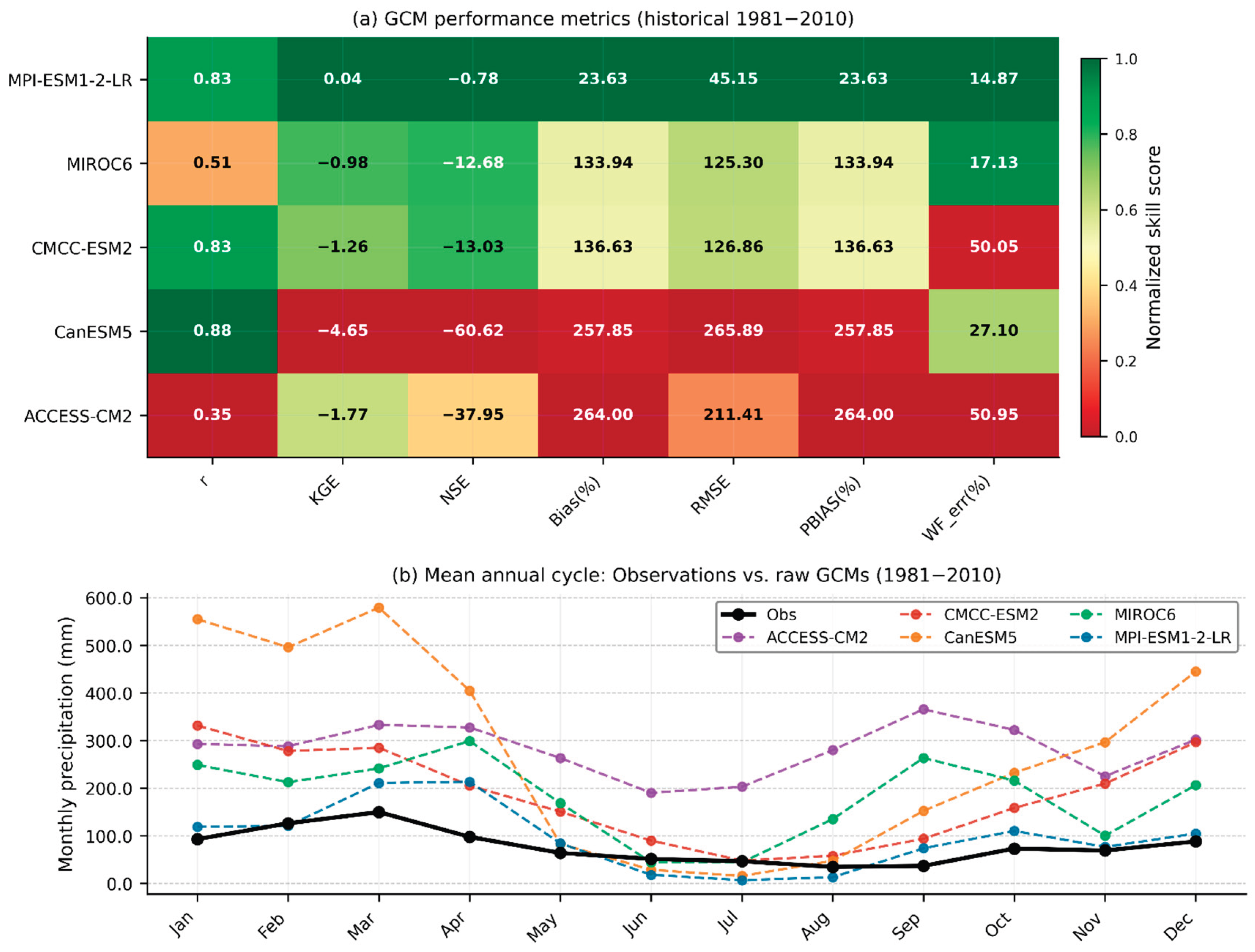
GCM performance metrics are summarized in Table 2. MPI-ESM1-2-LR ranked first by composite KGE–NSE–Pearson r score. All five models yield negative NSE and sub-optimal KGE values when evaluated against point-scale observations without prior bias correction, reflecting systematic wet biases intrinsic to coarse-resolution GCMs over complex orographic terrain rather than methodological deficiencies. MPI-ESM1-2-LR achieved the strongest temporal correlation (r = 0.830) and the smallest overestimation bias (PBIAS = 23.6%). CanESM5 and ACCESS-CM2 exhibited severe the largest wet biases, exceeding 250%, consistent with coarser effective resolution and known overestimation of convective precipitation in complex terrain by these models [31].
Figure 2.
Multi-metric evaluation of raw CMIP6 GCMs against SC-PREC4SA observations (1981–2010). (a) Normalized performance heatmap across seven evaluation metrics. (b) Mean annual precipitation cycle comparing the raw GCM outputs against the homogenized observational baseline.
Figure 2.
Multi-metric evaluation of raw CMIP6 GCMs against SC-PREC4SA observations (1981–2010). (a) Normalized performance heatmap across seven evaluation metrics. (b) Mean annual precipitation cycle comparing the raw GCM outputs against the homogenized observational baseline.
3.2. Independent Validation
Split-sample validation, in which the bias-correction transfer function was calibrated on 1981–2000 and evaluated against the withheld 2001–2010 period, confirmed genuine out-of-sample skill for every model (Table 3). Raw historical GCM output showed strongly negative NSE and KGE in the validation window for all five models (NSE from −1.2 to −71.7; KGE from −0.08 to −5.04), reflecting the same systematic wet bias documented in Section 3.1. After bias correction, KGE improved to 0.60–0.76 and percent bias fell to within ±10.5% of observed for every model, none of which had contributed to the calibration period. This out-of-sample improvement — obtained on data never used to fit the correction — indicates that the transfer function captures a genuine, transferable statistical relationship between model and station precipitation rather than simply reproducing its own calibration data.
3.3. Downscaled Precipitation: Annual and Monthly Changes
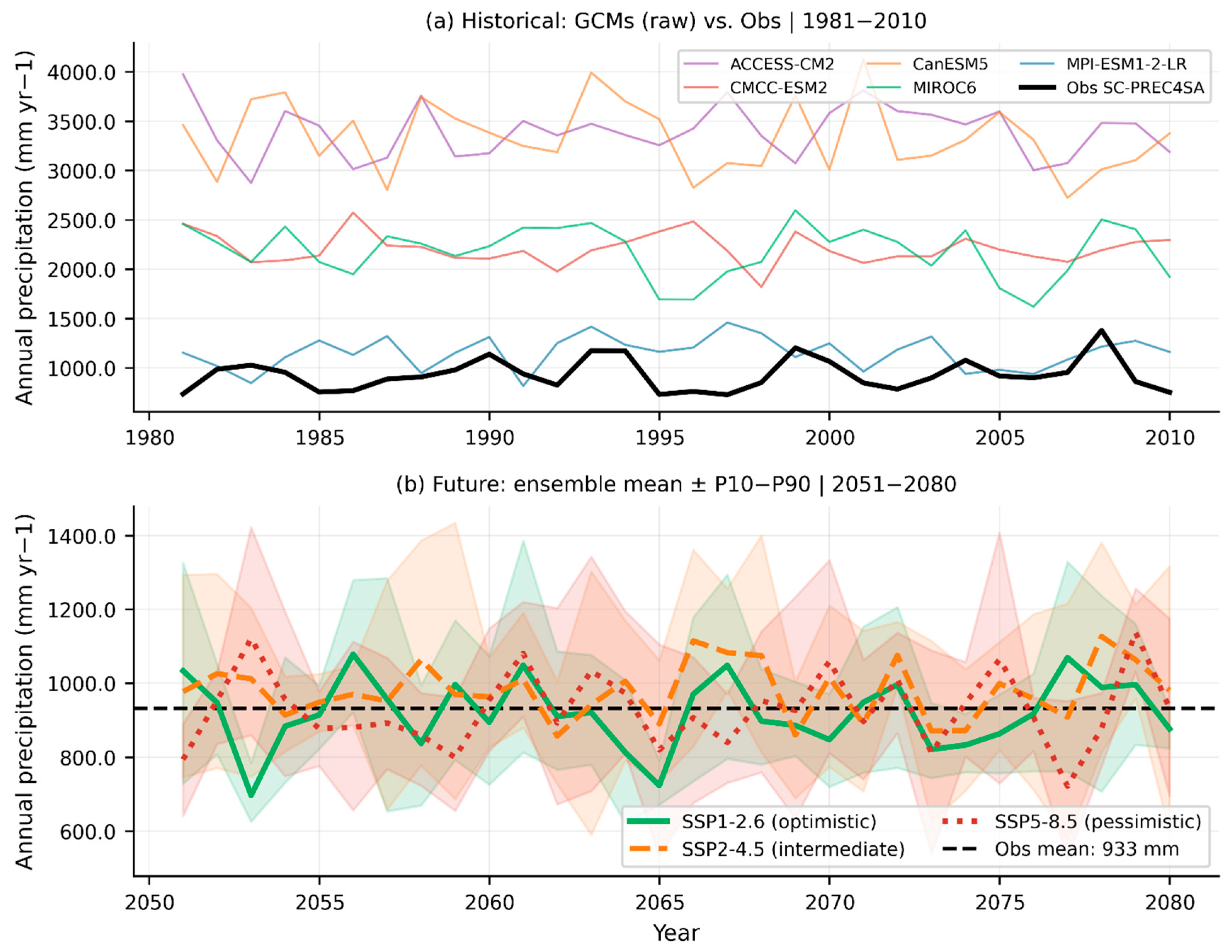
Quantile delta mapping produced modest and directionally mixed changes in ensemble-mean annual precipitation relative to the 932.6 mm year⁻¹ historical baseline (Table 4; Figure 3 and Figure 4). Under SSP1-2.6, the ensemble mean declined by −12.1 mm year⁻¹ (−1.3%; inter-model range 825–1016 mm year⁻¹). Under SSP2-4.5, the ensemble mean increased by +47.2 mm year⁻¹ (+5.1%; range 830–1080 mm year⁻¹). Under SSP5-8.5, the change was negligible at −3.3 mm year⁻¹ (−0.4%; range 783–1077 mm year⁻¹). At the level of individual models, CMCC-ESM2 and CanESM5 consistently projected decreases across all scenarios (−4.3% to −17.0%), whereas MIROC6 and MPI-ESM1-2-LR consistently projected increases (+4.0% to +16.6%); ACCESS-CM2, available only for SSP2-4.5, projected an increase of +16.3%. This split between consistently drying and consistently wetting models, more than the choice of emission scenario, governs the sign of the ensemble mean in any given pathway.
Figure 5.
Annual precipitation time series for raw GCMs versus observations and future downscaled projections. (a) Historical annual precipitation (1981–2010), raw CMIP6 outputs versus the homogenized SC-PREC4SA baseline. (b) Future downscaled ensemble mean precipitation with inter-model range under three SSP scenarios (2051–2080).
Figure 5.
Annual precipitation time series for raw GCMs versus observations and future downscaled projections. (a) Historical annual precipitation (1981–2010), raw CMIP6 outputs versus the homogenized SC-PREC4SA baseline. (b) Future downscaled ensemble mean precipitation with inter-model range under three SSP scenarios (2051–2080).
3.4. Changes in Precipitation Distribution and Wet-Day Frequency
Quantile distributions of daily precipitation for each scenario, computed from each model's own distribution before aggregation, track the observed distribution closely across nearly the full probability range under all three scenarios, with a modest upward shift confined to the uppermost quantiles (Figure 6a). Wet-day frequency showed modest, non-significant adjustments (individual models ranging from about 28% to 46% against an observed 36.8%), with no directional consensus across models under any scenario (Figure 6b). The monthly change heatmap (Figure 7) shows that the largest relative anomalies occur across individual models in austral autumn and winter (April–September), with several models projecting changes exceeding ±30% in a given month; inter-model agreement on the sign of change is generally lower in this season than during the primary wet season.
3.5. ETCCDI Extreme Precipitation Indices
ETCCDI indices (Table 5; Figure 8) indicate precipitation tail intensification across scenarios, most consistently for the fixed-day maxima and mean intensity indices. Rx1day ensemble means increase relative to the observed 40.5 mm, reaching 46.4 mm under SSP1-2.6, 46.6 mm under SSP2-4.5, and 52.2 mm under SSP5-8.5 (+14.6% to +28.9%). Rx5day increases from an observed 80.3 mm to 88.5–92.7 mm (+10.2% to +15.4%) across scenarios. SDII rises modestly from an observed 6.7 mm day⁻¹ to 6.7–7.3 mm day⁻¹. R95p increases from an observed 399 mm to 407–421 mm. Consecutive-day indices are more mixed: the annual-maximum CWD (8.7 days observed) increases to 11.2–13.7 days across scenarios without a clear ordering by scenario, and annual-maximum CDD (19.5 days observed) increases to 26.8–29.3 days across all three scenarios, indicating a lengthening of the longest annual dry spell alongside intensified peak-day rainfall.
3.6. Return-Period Analysis
Gumbel maximum-likelihood fits to the observed series yield a RP-10 of 54.2 mm day⁻¹ [95% CI: 47.7–59.7] and RP-50 of 67.6 mm day⁻¹ [95% CI: 58.1–75.4] (Table 5; Figure 9). Future ensemble-mean projections show systematic upward shifts: the RP-100 increases from the observed 73.2 mm day⁻¹ to 91.9 ± 10.3 mm day⁻¹ under SSP1-2.6, 88.3 ± 6.7 mm day⁻¹ under SSP2-4.5, and 107.5 ± 15.7 mm day⁻¹ under SSP5-8.5—increments of 26%, 21%, and 47%, respectively. A sensitivity check comparing Gumbel fits with and without the 99th-percentile cap on annual maxima showed a mean difference of only +0.6% in RP-100 across all 13 available model–scenario combinations, indicating the cap does not materially affect the reported return levels.
Comparing SSP2-4.5 against SSP5-8.5 with the Mann–Whitney U test applied directly to the four-to-five model point estimates yields no statistically significant difference at any return period (p = 0.111–0.190), a result of limited value given the very small number of independent realizations available to the test. Pooling the 500 bootstrap replicates generated for each model's confidence interval into a single per-scenario sample (~2000 values) and repeating the comparison yields a statistically significant difference at all three return periods (RP-10, RP-50, RP-100; p < 0.05), with higher medians under SSP5-8.5 than SSP2-4.5 at every return period considered (e.g., RP-50 medians of 79.5 mm versus 95.3 mm). The two tests answer related but distinct questions — whether the four-to-five model realizations differ, versus whether the pooled distributions of plausible return-level estimates differ — and their divergent outcomes illustrate how sensitive small multi-model ensemble comparisons can be to the way the comparison sample is constructed
3.7. Temporal Trend Analysis (Mann–Kendall)
Mann–Kendall trend analysis of the 30-year annual precipitation time series (2051–2080) revealed predominantly weak and non-significant trends across models and scenarios (Figure 10). Individual-model Kendall's τ ranged from −0.18 to +0.19, and the ensemble-mean τ from −0.01 to +0.06 across scenarios, none statistically significant at p < 0.05. Because the future series preserves each model's own simulated chronology (Section 2.5), this analysis evaluates genuine projected temporal structure rather than a resampled historical sequence; the absence of significant trends indicates that projected changes over 2051–2080 primarily manifest as shifts in the precipitation distribution rather than as a systematic monotonic trend within this 30-year window.
3.8. Uncertainty Decomposition and Model Consensus
The two-way variance decomposition (Figure 11a) shows that inter-model structural uncertainty is the largest single component of total projection variance in every calendar month, ranging from 51% to 93% (mean 75%). Scenario uncertainty is generally small, ranging from under 1% to 19% (mean 8%), and is largest in December–January. The model × scenario interaction term ranges from 0% to 33% (mean 17%) and exceeds 30% in January, March, and April; because only one realization exists per model–scenario combination, this term is confounded with single-realization noise and should not be read as an independent estimate of internal climate variability (Section 2.8).
Signal-to-noise ratios exceed 1.0 in only a small minority of month–scenario combinations, most notably January under SSP1-2.6 (Figure 12a), indicating that inter-model spread exceeds the ensemble-mean signal through most of the annual cycle. Applying an 80% model-agreement threshold — set to reflect the actual four-to-five model ensemble size rather than a fixed fraction calibrated to a six-model design — six of the 36 month–scenario combinations qualify as robust: January under SSP1-2.6, and February, March, June, September, and December under SSP2-4.5 (Figure 13). No month–scenario combination under SSP5-8.5 reaches this threshold. The concentration of robust signals under SSP2-4.5, and their absence under SSP5-8.5, is consistent with the higher inter-model dispersion evident in the return-period and annual-total results for the pessimistic scenario (Section 3.3 and Section 3.6).
3.9. Additional Hydroclimatic Diagnostics
Figure 14, Figure 15, Figure 16, Figure 17, Figure 18, Figure 19 and Figure 20 present further diagnostic of model performance, seasonal dynamics, and extreme precipitation behavior. The Taylor diagram (Figure 14) and multi-metric radar/ranking chart (Figure 15) summarize the historical evaluation of Section 3.1 in a complementary graphical form. Seasonal disaggregation (Figure 16) shows that all three scenarios track the observed seasonal means closely for DJF, MAM, and JJA, with the widest inter-model spread in SON. Dry- and wet-spell duration statistics (Figure 17) show mean consecutive dry-day spells lengthening modestly relative to the observed 3.8 days across all scenarios, with wider inter-model spread in SSP2-4.5. The percentile-bin analysis (Figure 18) shows a consistent pattern across models and scenarios: the lowest precipitation percentiles (P0–20) decrease substantially (ensemble mean −57% to −68%), while the upper percentiles (P95–100) are comparatively stable to slightly positive (+2% to +9% at the ensemble level, with individual models reaching +16%), consistent with a shift of probability mass away from light precipitation rather than a uniform intensification across the full distribution. Exceedance-probability curves (Figure 19) show that the frequency of days exceeding 10–50 mm day⁻¹ under future scenarios remains close to the observed frequency, with small absolute increases at higher thresholds under SSP2-4.5 and SSP5-8.5. The comprehensive statistics matrix (Figure 20) consolidates annual totals, spell statistics, and 50-year return levels across all model–scenario combinations into a single reference table.
The composite ranking in Figure 15b uses the mean of five normalized metrics (r, KGE, NSE, and inverted RMSE and Bias) as a broader visual summary of overall model fidelity, and can order models differently from Table 2, whose ranking is based on the three-metric criterion (KGE, NSE, and r ranks) defined in Section 2.3 and used for model selection throughout the study; both orderings place MPI-ESM1-2-LR first and CanESM5 among the lowest-performing models, and differ only in the relative position of CMCC-ESM2 and MIROC6.
4. Discussion
4.1. Key Findings in Context
Three principal findings emerge. First, the direction of ensemble-mean annual precipitation change is small and scenario-dependent (−1.3% to +5.1%), driven mainly by a consistent split between drying models (CMCC-ESM2, CanESM5) and wetting models (MIROC6, MPI-ESM1-2-LR) rather than by emission pathway. Second, extreme-event indicators intensify more consistently than the annual mean: Rx1day increases by 15–29% and 100-year return levels by 21–47% across scenarios, in line with regional syntheses documenting intensification of upper precipitation percentiles across the tropical Andes under warming [32]. Third, inter-model structural uncertainty dominates total projection variance in every calendar month (51–93%), substantially exceeding scenario uncertainty (under 1–19%).
By preserving each model's own projected daily chronology and the full distribution of observed precipitation intensity, the quantile delta mapping framework captures tail intensification that would not be visible from mean-change metrics alone. The projected +29% Rx1day increase under SSP5-8.5 falls within the 15–30% range documented in regional assessments for the tropical Andes at comparable levels of global warming [32]. Recent CMIP6-based assessments in other data-scarce and topographically complex settings have reported a similar pattern of pronounced extreme-index intensification alongside comparatively modest mean-annual change, in the Yangtze River basin [33] and across the Korean peninsula [34], reinforcing that return-period and extreme-index analyses, rather than mean-change metrics alone, should anchor climate-risk communication in this type of setting. The joint lengthening of the annual-maximum dry spell (CDD, +37–50%) alongside intensified 1-day and 5-day maxima is consistent with the compound-hazard framing of Zscheischler et al. [35], whereby reduced wet-day frequency combined with elevated per-event intensity can amplify flash-flood and soil-erosion risk in steep mountain watersheds, even where the annual water balance itself changes little.
The chronology-preserving quantile delta mapping procedure applied here is one of several established bias-correction strategies for daily precipitation [13]; it was selected over simpler mean-scaling and delta-change approaches because it corrects the full distribution rather than a single central-tendency statistic, and over more data-demanding multivariate or stochastic weather-generator approaches because it requires only single-site daily observations and single-realization GCM output, both of which are the practical constraint at this station. A direct quantitative comparison against alternative bias-correction families (e.g., multivariate approaches conditioned on atmospheric circulation analogs [36]) was outside the scope of the present single-station application and is identified as a priority direction in Section 4.5; the independent split-sample validation reported in Section 3.2 was carried out specifically to provide evidence of predictive skill in the absence of such a comparison.
4.2. Uncertainty Decomposition Implications
Inter-model structural uncertainty is the dominant component of total projection spread in all 12 calendar months, in contrast with mid-latitude findings where scenario uncertainty becomes comparable to or exceeds internal/model variability by mid-century [27]. This is consistent with the documented characteristics of tropical projections, where ENSO-driven decadal variability and inter-model differences in convective parameterization are large relative to the forced scenario signal. The practical implication is that, at this station, expanding the diversity of the GCM ensemble is likely to narrow decision-relevant uncertainty more effectively than further disaggregating emission scenarios.
4.3. Return Periods and Engineering Implications
The RP-100 increase from 73.2 mm day⁻¹ observed to 88.3–107.5 mm day⁻¹ across scenarios represents a 21–47% intensification of daily rainfall at this station under the return-period framework evaluated here. These are daily-resolution, single-station statistics, and their translation into specific drainage-infrastructure design values is not direct: municipal and hydraulic design standards are typically expressed in terms of sub-daily (e.g., 1-hour or shorter) intensity–duration–frequency curves, require the disaggregation of daily totals informed by local storm structure, and depend on spatially distributed precipitation inputs and hydrological or hydraulic modeling rather than a point estimate at a single station. The results presented here are accordingly best read as evidence of the direction and approximate magnitude of change in daily extreme precipitation at this station, providing a quantitative starting point for such downstream engineering analysis rather than a substitute for it. The bootstrap 95% confidence intervals reported in Table 6 give a probabilistic range for return-level estimates that explicitly incorporates GCM structural uncertainty, for use in that downstream analysis. The contrast between the two Mann–Whitney comparisons in Section 3.6 — non-significant on four-to-five point estimates, significant once bootstrap replicates are pooled across models — is itself an important practical finding: with an ensemble this small, whether a scenario comparison appears “significant” can depend as much on how the comparison sample is constructed as on the underlying climate signal, and any downstream design values should be drawn from the full multi-model distribution rather than from a single point-estimate comparison.
4.4. Limitations
Seven limitations qualify interpretation. First, the effective ensemble size is only four models for SSP1-2.6 and SSP5-8.5 and five for SSP2-4.5, following the unavailability of ACCESS-CM2 future data for two scenarios and of NorESM2-LR for the full ensemble; this constrains the statistical power of any cross-model or cross-scenario comparison. Second, the interaction term in the variance decomposition (Section 3.8) is confounded with single-realization noise and cannot be interpreted as an independent estimate of internal climate variability, which requires long, continuously evolving simulations to isolate. Third, SC-PREC4SA constitutes a single-point measurement, and the presented projections are representative of this station rather than of the surrounding region as a whole. Fourth, quantile delta mapping assumes that the statistical relationship between model and observed distributions used for bias correction remains valid under the level of warming considered; while chronology is preserved from the model's own future trajectory, the correction itself is a statistical transfer function whose stationarity cannot be independently verified. Fifth, the two-parameter Gumbel distribution, chosen over a three-parameter alternative for the reasons given in Section 2.7, may underestimate return levels if the true tail behavior of precipitation extremes at this station departs from the light-tailed Type I shape, particularly at return periods beyond those evaluated here (T > 100 years) [26]; a comparison against the (log-)Pearson Type III and GEV distributions, not undertaken here given the 30-year record length available, is identified as a priority check in Section 4.5. Sixth, the daily-resolution, single-station return levels reported here require sub-daily disaggregation, spatial extension, and hydrological or hydraulic modeling before they can inform specific drainage-infrastructure design values, as discussed in Section 4.3. Seventh, NorESM2-LR, IPSL-CM6A-LR, and EC-Earth3 were not available for inclusion in the present ensemble; their addition is identified as a priority for improving statistical power and inter-model diversity in future work.
4.5. Future Research Directions
Ensemble expansion to include NorESM2-LR, IPSL-CM6A-LR, and EC-Earth3 would improve statistical power for cross-model and cross-scenario comparisons. Comparison against multivariate bias-correction schemes conditioned on atmospheric circulation analogs [36] would help quantify the sensitivity of the results to the stationarity assumption discussed in Section 4.4. Spatial extension of the present pipeline to the broader SC-PREC4SA station network would enable distributed, rather than single-point, projections across the region, and would additionally allow direct comparison against CORDEX-CORE regional simulations as their daily precipitation archive for this domain becomes available (Section 2.2). Adoption of the generalized extreme value family or the (log-)Pearson Type III distribution with L-moment estimation would extend return-period reliability beyond the 100-year horizon evaluated here and test the sensitivity of the results to the Gumbel shape assumption noted in Section 4.4. Integration with a calibrated hydrological model, together with sub-daily disaggregation of the daily projections presented here, would be required before translating these station-level results into specific drainage-infrastructure design values.
5. Conclusions
A multi-model, multi-scenario quantile delta mapping framework was applied to five CMIP6 GCMs under SSP1-2.6, SSP2-4.5, and SSP5-8.5 at a high-altitude tropical station (2160 m a.s.l.), yielding five principal conclusions.
(1) GCM performance evaluation: MPI-ESM1-2-LR ranked first by composite KGE–NSE–Pearson r score (r = 0.830). All models exhibited positive wet biases of 24–264% in raw form. Negative NSE values are consistent with known limitations of coarse-resolution GCMs applied to point-scale observations over complex terrain; independent split-sample validation confirmed that the resulting bias correction achieves genuine out-of-sample skill (KGE improving from negative values to 0.60–0.76) rather than simply reproducing its own calibration data.
(2) Mean precipitation change: Ensemble-mean annual changes are modest and directionally mixed (−1.3% to +5.1%), governed principally by a consistent split between drying and wetting models rather than by emission scenario. No scenario supports a robust determination of net drying or wetting for the 2051–2080 window at this station.
(3) Extreme precipitation: ETCCDI indices indicate tail intensification that is more consistent across scenarios than the annual mean. Rx1day increases by 15–29%; the 100-year daily return level rises from 73.2 mm day⁻¹ to 88.3–107.5 mm day⁻¹. Translating these station-level, daily-resolution results into drainage-infrastructure design values would require sub-daily disaggregation, spatial extension beyond this single station, and hydrological or hydraulic modeling (Section 4.3). Concurrent lengthening of the annual-maximum dry spell characterizes a compound hazard of more intense but less evenly distributed precipitation.
(4) Uncertainty decomposition: Inter-model structural uncertainty is the dominant component of total projection variance in every calendar month (51–93%), substantially exceeding scenario uncertainty (under 1–19%). Expanding GCM ensemble diversity is likely to be a more effective lever for reducing decision-relevant uncertainty at this station than further disaggregating emission scenarios.
(5) Return-period sensitivity to comparison method: a Mann–Whitney comparison of SSP2-4.5 against SSP5-8.5 return levels is non-significant when applied to the small number of available model point estimates, but significant once bootstrap replicates are pooled across models — a methodological finding relevant to any small multi-model ensemble study of this kind, and a reminder that infrastructure design values should draw on the full multi-model distribution rather than a single pairwise comparison.
The documented pipeline, including its independent validation step, constitutes a transferable methodological framework for probabilistic precipitation projection at other data-scarce, high-altitude tropical stations across the Andes.
Key Findings:
- Non-monotonic annual response: ensemble-mean annual precipitation change does not scale with emission-pathway severity — SSP2-4.5 (intermediate) shows the largest projected increase (+5.1%), while SSP1-2.6 (optimistic) and SSP5-8.5 (pessimistic) show small, opposite-signed changes (−1.3% and −0.4%), reflecting a consistent split between drying and wetting models rather than a scenario effect.
- Extreme intensification outpaces the annual mean: despite a near-neutral annual-mean change under SSP5-8.5 (−0.4%), this scenario shows the strongest intensification of extremes among the three (Rx1day +28.9%; 100-year return level +47%, from 73.2 to 107.5 mm day⁻¹), confirming that extreme-index and return-period analysis, not mean-change metrics alone, should anchor risk assessment at this station .
- Return-level differences depend on how the comparison is constructed: a Mann–Whitney test on the four-to-five model point estimates alone finds no significant difference between SSP2-4.5 and SSP5-8.5 (p = 0.111–0.190), but pooling each model's bootstrap replicates (~2000 samples per scenario) reveals a statistically significant difference at every return period evaluated, with higher return levels under SSP5-8.5.
- Model uncertainty dominates: inter-model structural differences account for 51–93% (mean 75%) of total monthly projection variance, far exceeding scenario uncertainty (under 1–19%, mean 8%), indicating that expanding GCM ensemble diversity would narrow decision-relevant uncertainty more than further disaggregating emission scenarios.
- Validated downscaling: independent split-sample validation (calibration 1981–2000, evaluation on the withheld 2001–2010 period) confirms genuine out-of-sample skill of the quantile delta mapping procedure, with Kling–Gupta efficiency improving from negative values for every raw model to 0.60–0.76 after correction.
Funding
This research was financially supported by the Universidad Técnica Particular de Loja (UTPL, RUC: 1190068729001) for the acquisition of the computational resources used in this study, managed through the Hydraulics Laboratory of the aforementioned Research Group. The Universidad Técnica Particular de Loja – Ecuador also covered the Article Processing Charge (APC).
Institutional Review Board Statement
Not applicable.
Informed Consent Statement
Not applicable.
Data Availability Statement
CMIP6 model data are publicly available via the Pangeo CMIP6 cloud catalog (https://pangeo-data.github.io/pangeo-cmip6-cloud/). SC-PREC4SA observational data are available from Huerta et al. (2025, Scientific Data) [29]. Appendix A describes the essential structure of the analysis code that implements the algorithm.
Acknowledgments
The author gratefully acknowledges the institutional support of the Universidad Técnica Particular de Loja (UTPL), through the Research Group R&D for the Sustainability of the Urban and Rural Water Cycle (Department of Civil Engineering, Architecture and Geosciences), which made available the computational resources essential for this study.
Conflicts of Interest
The author declares no conflict of interest.
Abbreviations
The following abbreviations are used in this manuscript:
| CI | Confidence Interval |
| CMIP6 | Coupled Model Intercomparison Project Phase 6 |
| CDD | Consecutive Dry Days |
| CWD | Consecutive Wet Days |
| DJF | December–January–February |
| ENSO | El Niño–Southern Oscillation |
| ETCCDI | Expert Team on Climate Change Detection and Indices |
| GCM | General Circulation Model |
| GEV | Generalized Extreme Value |
| ITCZ | Intertropical Convergence Zone |
| JJA | June–July–August |
| KGE | Kling–Gupta Efficiency |
| MAM | March–April–May |
| NAS | Northern Andes and Sierra ecoregion |
| NSE | Nash–Sutcliffe Efficiency |
| PBIAS | Percent Bias |
| QDM | Quantile Delta Mapping |
| RP | Return Period |
| R95p | Total precipitation on very wet days (95th percentile threshold) |
| Rx1day | Annual maximum 1-day precipitation |
| Rx5day | Annual maximum 5-day accumulated precipitation |
| SC-PREC4SA | South American Climate daily PRECipitation 4 Station Assessment |
| SDII | Simple Daily Intensity Index |
| SON | September–October–November |
| SSP | Shared Socioeconomic Pathway |
| S/N | Signal-to-Noise ratio |
Appendix A. Condensed Reproducible Pipeline
The following algorithms summarize, at implementation level of detail, the computational steps underlying the analyses reported in Section 2 and Section 3: data preparation (A1), GCM performance evaluation (A2), independent split-sample validation (A3), quantile delta mapping downscaling (A4), ETCCDI extreme indices (A5), extreme-value analysis (A6), the two-way uncertainty decomposition (A7), and trend analysis (A8). This summary is sufficient to assess and reproduce the methodology from the equations given in Section 2. The pipeline is deterministic under random_state = 42; executing it against the SC-PREC4SA observations Huerta et al. [29].
| Algorithm A1. Data preparation |
| 1. Load the SC-PREC4SA daily series for station M0033; restrict to 1981-01-01 to 2010-12-31; confirm zero missing values. 2. Query the Pangeo CMIP6 catalog for the 'historical' and three SSP experiments, variable pr, table 'day', realization r1i1p1f1, for the five retained models. 3. Extract the grid cell nearest to the station coordinates; convert flux units (kg m-2 s-1) to mm/day; restrict historical data to 1981-2010 and future data to 2051-2080 per scenario. |
| Algorithm A2. GCM performance evaluation (Sec. 2.3, Eqs. 1-3) |
| 1. Aggregate observed and simulated daily series to mean monthly totals. 2. Compute r, Bias, RMSE, MAE, NSE, KGE, PBIAS, wet-day-frequency error, and the 95th-percentile ratio for each model against observations. 3. Rank models by the summed rank of KGE, NSE, and r (ascending); select the top-ranked model as the evaluation reference. |
| Algorithm A3. Independent split-sample validation (Sec. 2.4) |
| 1. Partition the observed and historical-model record into a calibration window (1981-2000) and a validation window (2001-2010). 2. Fit the bias-correction transfer function (Algorithm A4) using the calibration window only. 3. Apply the fitted transfer function to the model's own validation-window data; compute NSE, KGE, and PBIAS against observations for the withheld period. |
| Algorithm A4. Quantile delta mapping downscaling (Sec. 2.5, Eq. 4) |
| For each calendar month independently: 1. Estimate empirical quantile functions of the observed, historical-model, and future-model daily series (1001-point grid). 2. For each future-model day, take its own empirical rank tau within the future- model distribution for that month. 3. Evaluate the historical-model and observed quantile functions at tau; form the relative and absolute perturbation factors, RF(tau) and AF(tau) (Sec. 2.5), clipping RF to [0.1, 3.0] to bound the correction near the dry/wet transition. 4. Blend RF and AF by the observed magnitude at tau, following the linear threshold scheme between 1.0 and 5.0 mm/day described in Sec. 2.5. 5. Assign the corrected value to the future day's own real calendar date, so the model's simulated chronology is preserved (not a resampled historical one). Applied independently to every retained model x scenario combination. |
| Algorithm A5. ETCCDI extreme indices and spell statistics (Sec. 2.6, Table 1) |
| Per year: compute Rx1day, Rx5day, SDII, R95p, and the annual-maximum consecutive wet/dry run lengths (CWD, CDD) from standard run-length encoding of the wet/dry day indicator; average indices over the 30-year window. Mean and 90th-percentile spell duration are computed separately from the full run-length distribution. |
| Algorithm A6. Extreme-value analysis (Sec. 2.7, Eq. 11) |
| 1. Take annual maxima of the (downscaled) daily series; cap at the 99th percentile of the annual-maxima series (sensitivity checked against the uncapped fit). 2. Fit the Gumbel distribution by maximum likelihood; evaluate return levels at T = 2, 5, 10, 20, 50, 100 years (Eq. 11). 3. Resample the annual maxima with replacement (500 draws) to build bootstrap 95% confidence intervals for each return level. 4. Compare SSP2-4.5 and SSP5-8.5 with the Mann-Whitney U test, both on the raw per-model point estimates and on the pooled bootstrap replicates. |
| Algorithm A7. Two-way uncertainty decomposition (Sec. 2.8) |
| For each calendar month, build the scenario x model table of mean monthly values; compute the total sum of squares around the grand mean independently, then the between-scenario and between-model sums of squares from the marginal means; the interaction is the remainder. Report each term as a percentage of the independently computed total (not of the sum of the other two terms). |
| Algorithm A8. Trend analysis (Sec. 3.7) |
| Standard Mann-Kendall test with Sen's slope estimator (Mann, 1945; Kendall, 1975; Sen, 1968), applied to the annual totals of the chronology-preserving downscaled series (Algorithm A4) for each model and the ensemble mean. |
The snippet below shows the core transfer-function logic to illustrate how Eq. (4) and the threshold-blending scheme of Sec. 2.5 are implemented.
| # _______________________ def quantile_delta_mapping_daily(obs, hist, fut, t_lo=1.0, t_hi=5.0): """Chronology-preserving quantile delta mapping (Eq. 4).""" q = np.linspace(0, 1, 1001) out = pd.Series(index=fut.index, dtype=float) for m in range(1, 13): o, h, f = (s[s.index.month == m] for s in (obs, hist, fut)) if o.empty or h.empty or f.empty: continue q_obs, q_hist = o.quantile(q).values, h.quantile(q).values tau = f.rank(pct=True).values # future day's own rank x_hist = np.interp(tau, q, q_hist) x_obs = np.interp(tau, q, q_obs) rel = np.clip(f.values / (x_hist + 1e-6), 0.1, 3.0) # Sec. 2.5 add = f.values - x_hist w = np.clip((x_obs - t_lo) / (t_hi - t_lo), 0, 1) factor = np.where(x_obs > t_hi, rel, rel * w + (1 - w)) offset = np.where(x_obs < t_lo, add, add * (1 - w)) out.loc[f.index] = np.maximum(x_obs * factor + offset, 0) return out.dropna() # indexed by the future day's own real date # _______________________ |
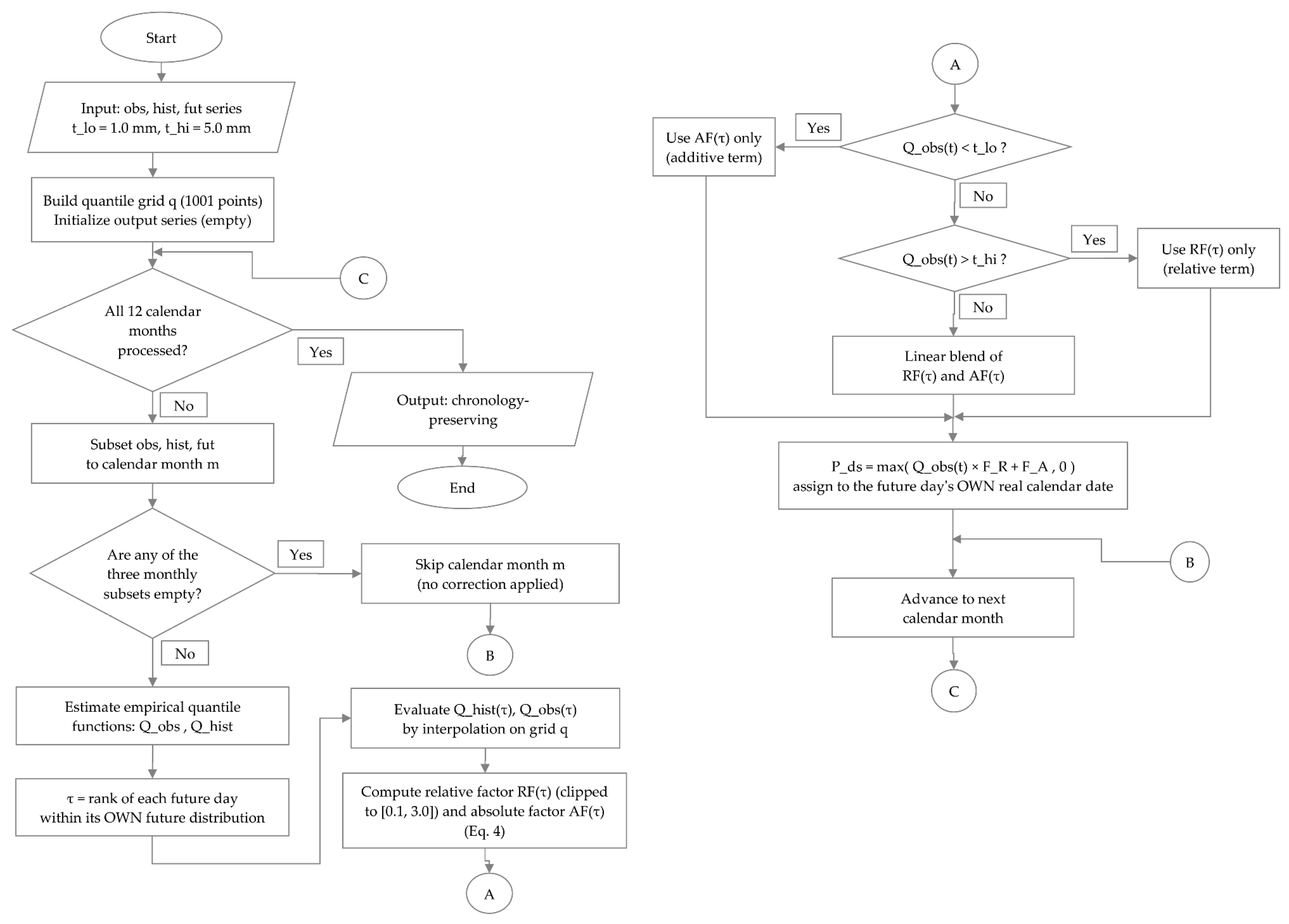
Figure A1 presents a general, high-level overview of the quantile delta mapping (QDM) procedure, and Figure A2 presents the corresponding detailed flowchart of the same procedure as implemented in Listing A1 and formalized in Equation (4).
Figure A1.
General overview of the quantile delta mapping (QDM) procedure. For each calendar month, empirical quantile functions are estimated from the observed, historical-model, and future-model series; each future value is located within its own future-model distribution; the corresponding historical and observed quantiles are evaluated at that rank; and the relative and absolute correction factors are combined according to Equation (4) before the corrected value is assigned to its own real calendar date. This sequence is repeated for every future value before the final chronology-preserving downscaled series is produced.
Figure A1.
General overview of the quantile delta mapping (QDM) procedure. For each calendar month, empirical quantile functions are estimated from the observed, historical-model, and future-model series; each future value is located within its own future-model distribution; the corresponding historical and observed quantiles are evaluated at that rank; and the relative and absolute correction factors are combined according to Equation (4) before the corrected value is assigned to its own real calendar date. This sequence is repeated for every future value before the final chronology-preserving downscaled series is produced.
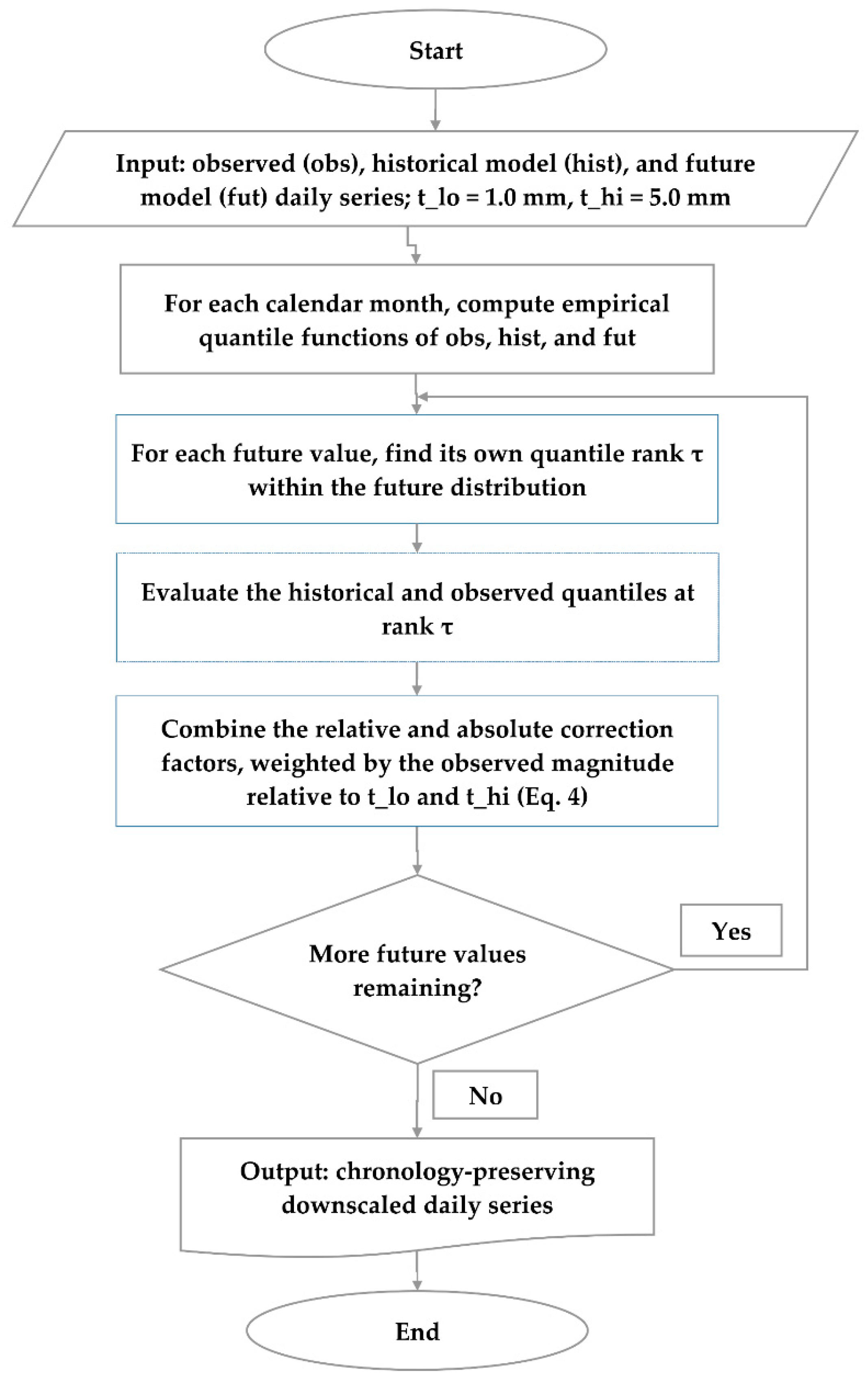
Figure A2 details the conditional structure of the correction factors, showing explicitly how the choice between the additive factor AF(τ), the relative factor RF(τ), and their linear blend depends on the magnitude of the observed value relative to the thresholds t_lo and t_hi, and how an empty monthly subset is skipped rather than forced through an ill-defined transfer function.
Figure A2.
Detailed flowchart of the quantile delta mapping algorithm implemented in Listing A1, illustrating the complete decision logic for computing each corrected value, P_ds.
Figure A2.
Detailed flowchart of the quantile delta mapping algorithm implemented in Listing A1, illustrating the complete decision logic for computing each corrected value, P_ds.
References
- IPCC. Climate Change 2021: The Physical Science Basis; Masson-Delmotte, V., et al., Eds.; Cambridge University Press: Cambridge, UK, 2021. [Google Scholar] [CrossRef]
- Trenberth, K.E.; Dai, A.; Rasmussen, R.M.; Parsons, D.B. The changing character of precipitation. Bull. Am. Meteorol. Soc. 2003, 84, 1205–1218. [Google Scholar] [CrossRef]
- Vuille, M.; Carey, M.; Huggel, C.; Buytaert, W.; Rabatel, A.; Jacobsen, D.; Soruco, A.; Villacis, M.; Yarleque, C.; Timm, O.E.; et al. Rapid decline of snow and ice in the tropical Andes. Earth-Sci. Rev. 2018, 176, 195–213. [Google Scholar] [CrossRef]
- Espinoza, J.C.; Garreaud, R.; Poveda, G.; Arias, P.A.; Molina-Carpio, J.; Masiokas, M.; Vignola, R.; Rosas, J. Hydroclimate of the Andes Part I: Main Climatic Features. Front. Earth Sci. 2020, 8, 64. [Google Scholar] [CrossRef]
- CRED/EM-DAT. EM-DAT: The OFDA/CRED International Disaster Database. Université catholique de Louvain (UCL) — CRED. 2020. Available online: https://www.emdat.be.
- Viviroli, D.; Dürr, H. H.; Messerli, B.; Meybeck, M.; Weingartner, R. Mountains of the world, water towers for humanity: Typology, mapping, and global significance. Water Resour. Res. 2007, 43(7). [Google Scholar] [CrossRef]
- Kundzewicz, Z.W.; Krysanova, V.; Benestad, R.E.; Hov, Ø.; Piniewski, M.; Otto, I.M. Uncertainty in climate change impacts on water resources. Environ. Sci. Policy 2018, 79, 1–8. [Google Scholar] [CrossRef]
- Bendix, J.; Rollenbeck, R.; Reudenbach, C. Diurnal patterns of rainfall in a tropical Andean valley of southern Ecuador. Int. J. Climatol. 2006, 26, 829–846. [Google Scholar] [CrossRef]
- Garreaud, R.D.; Vuille, M.; Compagnucci, R.; Marengo, J. Present-day South American climate. Palaeogeogr. Palaeoclimatol. Palaeoecol. 2009, 281, 180–195. [Google Scholar] [CrossRef]
- Vuille, M.; Bradley, R.S.; Keimig, F. Climate variability in the Andes of Ecuador and its relation to tropical Pacific and Atlantic sea surface temperature anomalies. J. Clim. 2000, 13, 2520–2535. [Google Scholar] [CrossRef]
- Bendix, J.; Trachte, K.; Cermak, J.; Rollenbeck, R.; Nauß, T. Formation of convective clouds at the foothills of the tropical eastern Andes (south Ecuador). J. Appl. Meteorol. Climatol. 2009, 48, 1682–1695. [Google Scholar] [CrossRef]
- Wilby, R.L.; Dawson, C.W.; Barrow, E.M. SDSM — a decision support tool for the assessment of regional climate change impacts. Environ. Model. Softw. 2002, 17, 145–157. [Google Scholar] [CrossRef]
- Maraun, D.; Widmann, M. Statistical Downscaling and Bias Correction for Climate Research; Cambridge University Press: Cambridge, UK, 2018; ISBN 9781107588783. [Google Scholar]
- Maraun, D.; Wetterhall, F.; Ireson, A.M.; Chandler, R.E.; Kendon, E.J.; Widmann, M.; et al. Precipitation downscaling under climate change: Recent developments to bridge the gap between dynamical models and the end user. Rev. Geophys. 2010, 48, RG3003. [Google Scholar] [CrossRef]
- Li, H.; Sheffield, J.; Wood, E.F. Bias correction of monthly precipitation and temperature fields from IPCC AR4 models using equidistant quantile matching. J. Geophys. Res. Atmos. 2010, 115, D10101. [Google Scholar] [CrossRef]
- Cannon, A.J.; Sobie, S.R.; Murdock, T.Q. Bias correction of GCM precipitation by quantile mapping: How well do methods preserve changes in quantiles and extremes? J. Clim. 2015, 28, 6938–6959. [Google Scholar] [CrossRef]
- O’Neill, B.C.; Tebaldi, C.; van Vuuren, D.P.; Eyring, V.; Friedlingstein, P.; Hurtt, G.; et al. The Scenario Model Intercomparison Project (ScenarioMIP) for CMIP6. Geosci. Model Dev. 2016, 9, 3461–3482. [Google Scholar] [CrossRef]
- Giustarini, L.; Schumann, G.J.-P.; Kettner, A.J.; Smith, A.; Nawrotzki, R. Simulating Changes in Hydrological Extremes—Future Scenarios for Morocco. Water 2023, 15, 2722. [Google Scholar] [CrossRef]
- Zeng, L.; Bi, H.; Li, Y.; Liu, X.; Li, S.; Chen, J. Nonstationary Annual Maximum Flood Frequency Analysis Using a Conceptual Hydrologic Model with Time-Varying Parameters. Water 2022, 14, 3959. [Google Scholar] [CrossRef]
- Gleckler, P.J.; Taylor, K.E.; Doutriaux, C. Performance metrics for climate models. J. Geophys. Res. Atmos. 2008, 113, D06104. [Google Scholar] [CrossRef]
- Gupta, H.V.; Kling, H.; Yilmaz, K.K.; Martinez, G.F. Decomposition of the mean squared error and NSE performance criteria: Implications for improving hydrological modelling. J. Hydrol. 2009, 377, 80–91. [Google Scholar] [CrossRef]
- Nash, J.E.; Sutcliffe, J.V. River flow forecasting through conceptual models part I — A discussion of principles. J. Hydrol. 1970, 10, 282–290. [Google Scholar] [CrossRef]
- Taylor, K.E. Summarizing multiple aspects of model performance in a single diagram. J. Geophys. Res. Atmos. 2001, 106, 7183–7192. [Google Scholar] [CrossRef]
- Zhang, X.; Alexander, L.; Hegerl, G.C.; Jones, P.; Tank, A.K.; Peterson, T.C.; Trewin, B.; Zwiers, F.W. Indices for monitoring changes in extremes based on daily temperature and precipitation data. WIREs Clim. Change 2011, 2, 851–870. [Google Scholar] [CrossRef]
- Donat, M.G.; Alexander, L.V.; Yang, H.; Durre, I.; Vose, R.; Dunn, R.J.H.; Willett, K.M.; Aguilar, E.; Brunet, M.; Caesar, J.; et al. Updated analyses of temperature and precipitation extreme indices: HadEX2. J. Geophys. Res. Atmos. 2013, 118, 2098–2118. [Google Scholar] [CrossRef]
- Katz, R.W.; Parlange, M.B.; Naveau, P. Statistics of extremes in hydrology. Adv. Water Resour. 2002, 25, 1287–1304. [Google Scholar] [CrossRef]
- Hawkins, E.; Sutton, R. The potential to narrow uncertainty in regional climate predictions. Bull. Am. Meteorol. Soc. 2009, 90, 1095–1107. [Google Scholar] [CrossRef]
- Dinerstein, E.; Olson, D.; Joshi, A.; Vynne, C.; Burgess, N.D.; Wikramanayake, E.; Hahn, N.; Palminteri, S.; Hedao, P.; Noss, R.; et al. An Ecoregion-Based Approach to Protecting Half the Terrestrial Realm. BioScience 2017, 67, 534–545. [Google Scholar] [CrossRef] [PubMed]
- Huerta, A.; Serrano-Notivoli, R.; Brönnimann, S. SC-PREC4SA: A serially complete daily precipitation dataset for South America. Sci. Data 2025, 12(1), 1006. [Google Scholar] [CrossRef] [PubMed]
- Ehret, U.; Zehe, E.; Wulfmeyer, V.; Warrach-Sagi, K.; Liebert, J. HESS Opinions: Should we apply bias correction to global and regional climate model data? Hydrol. Earth Syst. Sci. 2012, 16, 3391–3404. [Google Scholar] [CrossRef]
- Perkins, S.E.; Pitman, A.J.; Holbrook, N.J.; McAneney, J. Evaluation of the AR4 Climate Models’ Simulated Daily Maximum Temperature, Minimum Temperature, and Precipitation over Australia. J. Clim. 2007, 20, 4356–4376. [Google Scholar] [CrossRef]
- Poveda, G.; Espinoza, J.C.; Zuluaga, M.D.; Solman, S.A.; Garreaud, R.; van Oevelen, P.J. High Impact Weather Events in the Andes. Front. Earth Sci. 2020, 8, 162. [Google Scholar] [CrossRef]
- Xu, W.; Li, Q.; Wang, M.; Yang, S.; Chen, Y.; Zou, Y. Projections of Mean and Extreme Precipitation Using the CMIP6 Model: A Study of the Yangtze River Basin in China. Water 2023, 15, 3043. [Google Scholar] [CrossRef]
- Kim, S.; Shin, J.-Y.; Heo, J.-H. Assessment of Future Rainfall Quantile Changes in South Korea Based on a CMIP6 Multi-Model Ensemble. Water 2025, 17, 894. [Google Scholar] [CrossRef]
- Zscheischler, J.; Martius, O.; Westra, S.; Bevacqua, E.; Raymond, C.; Horton, R.M.; van den Hurk, B.; AghaKouchak, A.; Jézéquel, A.; Mahecha, M.D.; et al. A typology of compound weather and climate events. Nat. Rev. Earth Environ. 2020, 1, 333–347. [Google Scholar] [CrossRef]
- Vrac, M.; Friederichs, P. Multivariate—intervariable, spatial, and temporal—bias correction. J. Clim. 2015, 28, 218–237. [Google Scholar] [CrossRef]
Figure 1.
Observed baseline precipitation climatology at La Argelia station, Loja, Ecuador (1981–2010) derived from the homogenized SC-PREC4SA dataset. (a) Daily precipitation time series (mm day⁻¹). (b) Mean monthly precipitation cycle with ±1 standard deviation.
Figure 1.
Observed baseline precipitation climatology at La Argelia station, Loja, Ecuador (1981–2010) derived from the homogenized SC-PREC4SA dataset. (a) Daily precipitation time series (mm day⁻¹). (b) Mean monthly precipitation cycle with ±1 standard deviation.
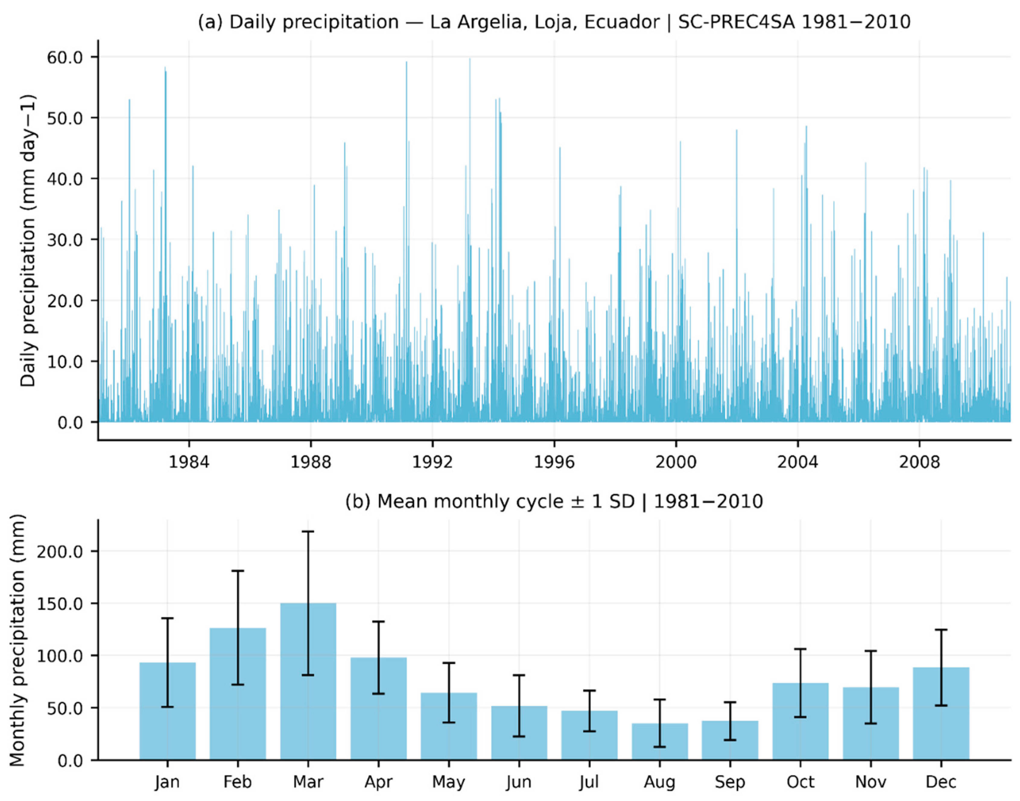
Figure 3.
Monthly precipitation annual cycle: observed (1981–2010, black) versus downscaled ensemble mean (2051–2080) under (a) SSP1-2.6, (b) SSP2-4.5, and (c) SSP5-8.5. Shaded envelope = 10th–90th percentile across each model's own monthly climatology; individual model lines shown in muted colors.
Figure 3.
Monthly precipitation annual cycle: observed (1981–2010, black) versus downscaled ensemble mean (2051–2080) under (a) SSP1-2.6, (b) SSP2-4.5, and (c) SSP5-8.5. Shaded envelope = 10th–90th percentile across each model's own monthly climatology; individual model lines shown in muted colors.
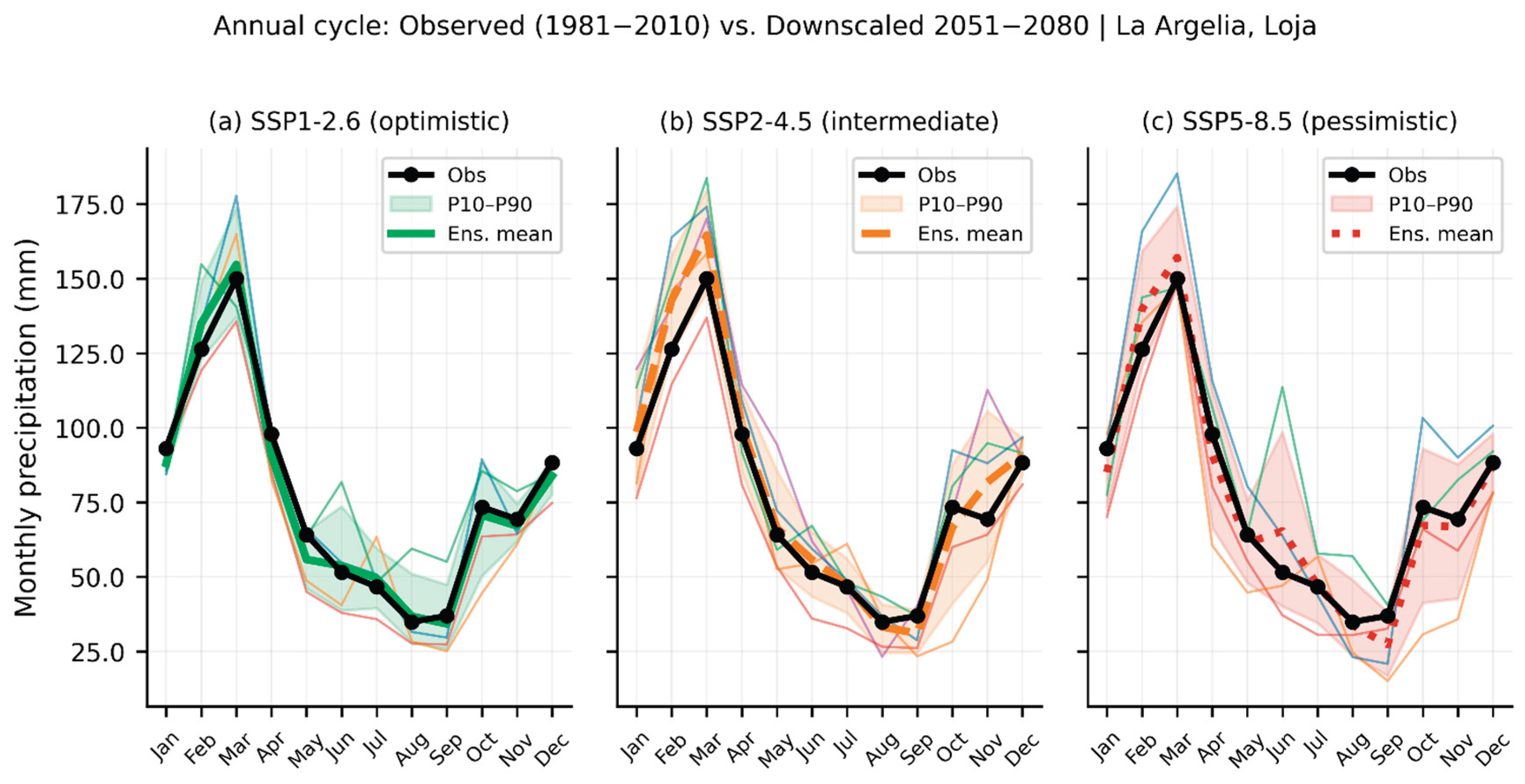
Figure 4.
Scenario comparison of monthly precipitation deltas and annual totals. (a) Ensemble-mean monthly precipitation change (Δ mm month⁻¹) relative to the 1981–2010 baseline. (b) Annual total precipitation per scenario and model (circles = individual models; diamond = ensemble mean; whiskers = inter-model interquartile range; dashed line = observed mean of 932.6 mm year⁻¹).
Figure 4.
Scenario comparison of monthly precipitation deltas and annual totals. (a) Ensemble-mean monthly precipitation change (Δ mm month⁻¹) relative to the 1981–2010 baseline. (b) Annual total precipitation per scenario and model (circles = individual models; diamond = ensemble mean; whiskers = inter-model interquartile range; dashed line = observed mean of 932.6 mm year⁻¹).
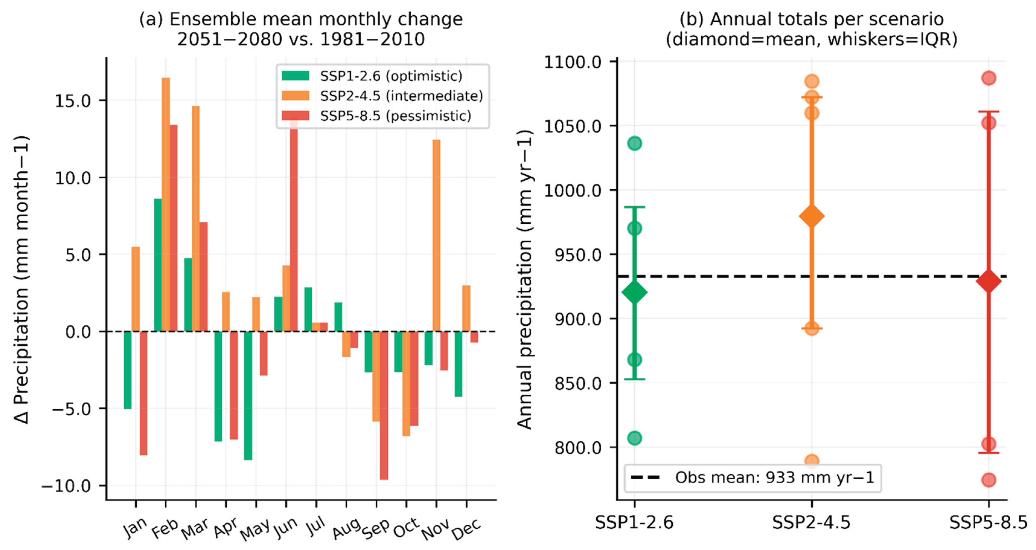
Figure 6.
Quantile distribution shifts and wet-day frequency alterations under future scenarios. (a) Log-scale quantile distribution of daily precipitation, observed baseline (1981–2010) versus the downscaled ensemble per scenario (2051–2080); shading denotes the 10th–90th percentile across each model's own quantile function. (b) Wet-day frequency (>1 mm day⁻¹) per scenario and model (diamond = ensemble mean; whiskers = inter-model interquartile range; dashed line = observed baseline of 36.8%).
Figure 6.
Quantile distribution shifts and wet-day frequency alterations under future scenarios. (a) Log-scale quantile distribution of daily precipitation, observed baseline (1981–2010) versus the downscaled ensemble per scenario (2051–2080); shading denotes the 10th–90th percentile across each model's own quantile function. (b) Wet-day frequency (>1 mm day⁻¹) per scenario and model (diamond = ensemble mean; whiskers = inter-model interquartile range; dashed line = observed baseline of 36.8%).
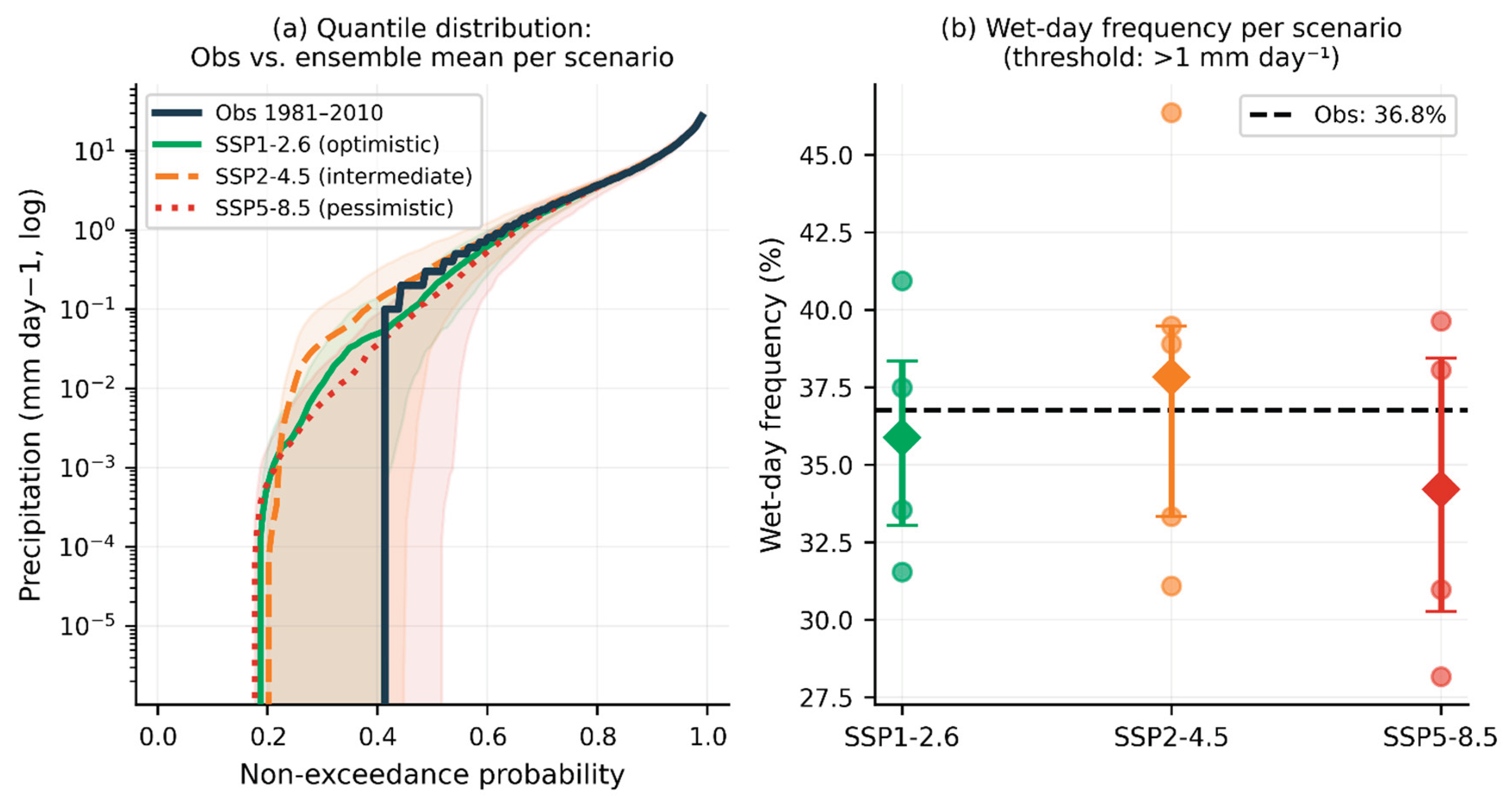
Figure 7.
Monthly precipitation change (%) per model and scenario (2051–2080 vs. 1981–2010), organized by scenario: (a) SSP1-2.6, (b) SSP2-4.5, and (c) SSP5-8.5. Each panel displays individual GCM rows alongside the ensemble mean (ENS, bottom row). Color scale: red = decrease, blue = increase.
Figure 7.
Monthly precipitation change (%) per model and scenario (2051–2080 vs. 1981–2010), organized by scenario: (a) SSP1-2.6, (b) SSP2-4.5, and (c) SSP5-8.5. Each panel displays individual GCM rows alongside the ensemble mean (ENS, bottom row). Color scale: red = decrease, blue = increase.
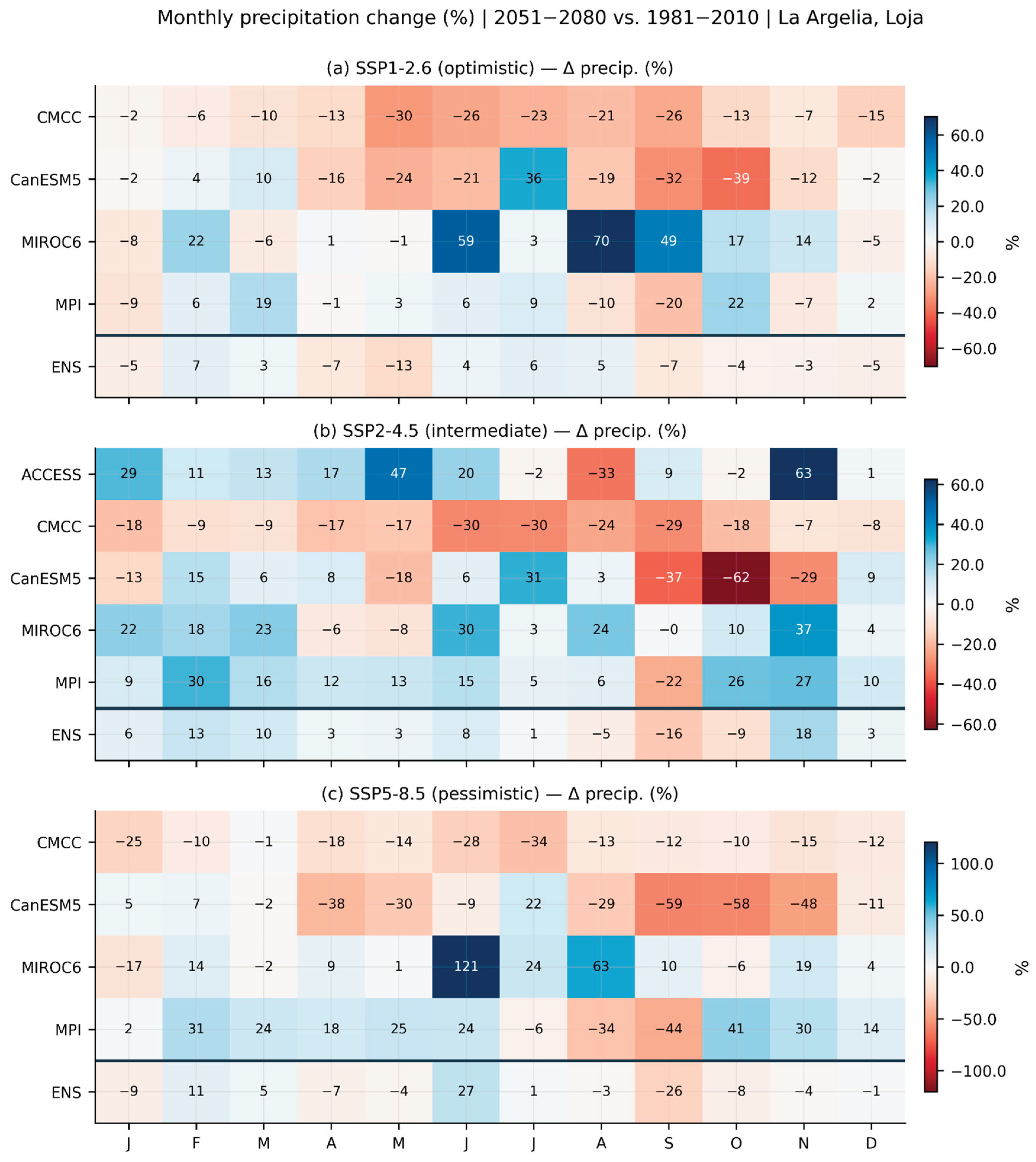
Figure 8.
ETCCDI extreme precipitation indices for 2051–2080 versus observed baseline (dashed) at La Argelia station: (a) Rx1day, (b) Rx5day, (c) SDII, (d) R95p, (e) CWD, (f) CDD. Bars represent ensemble mean; whiskers represent inter-model interquartile range - IQR.
Figure 8.
ETCCDI extreme precipitation indices for 2051–2080 versus observed baseline (dashed) at La Argelia station: (a) Rx1day, (b) Rx5day, (c) SDII, (d) R95p, (e) CWD, (f) CDD. Bars represent ensemble mean; whiskers represent inter-model interquartile range - IQR.
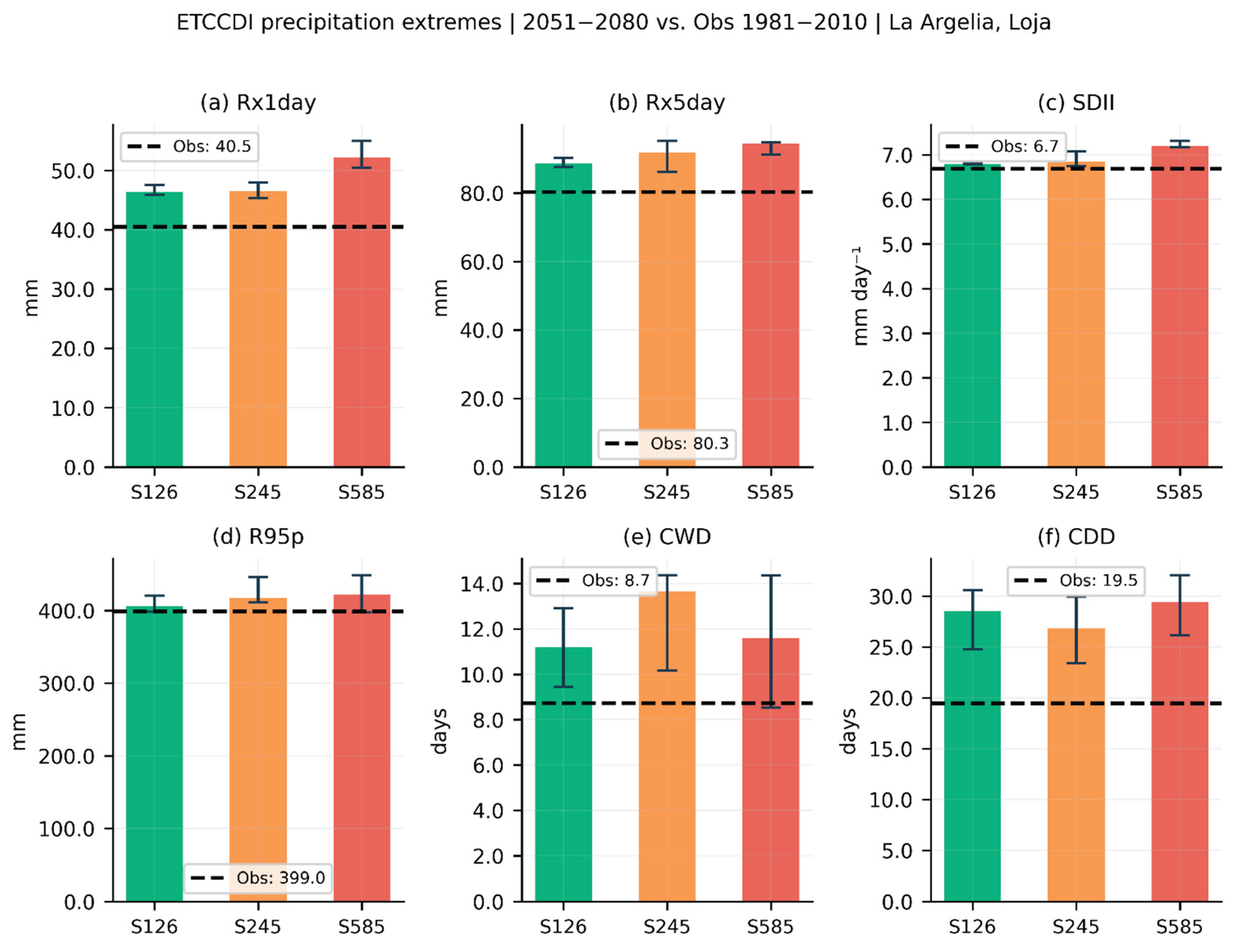
Figure 9.
Extreme event return periods fitted via the Gumbel distribution with bootstrap 95% confidence intervals for annual daily maxima (2051–2080 vs. observed 1981–2010), for (a) SSP1-2.6, (b) SSP2-4.5, and (c) SSP5-8.5.
Figure 9.
Extreme event return periods fitted via the Gumbel distribution with bootstrap 95% confidence intervals for annual daily maxima (2051–2080 vs. observed 1981–2010), for (a) SSP1-2.6, (b) SSP2-4.5, and (c) SSP5-8.5.
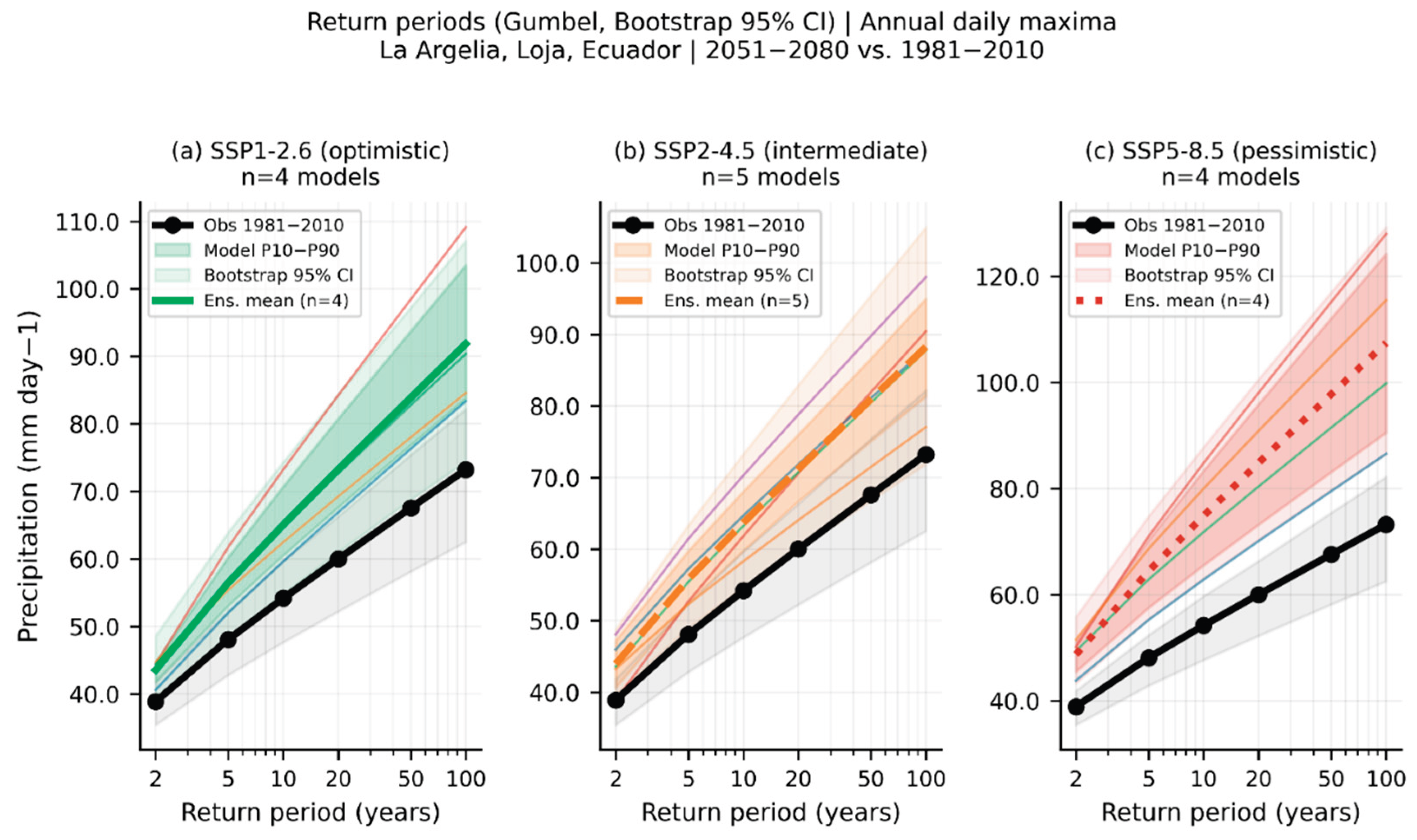
Figure 10.
Non-parametric trend analysis (Mann–Kendall) with Sen’s slope estimators for annual precipitation (2051–2080), organized by scenario: (a) SSP1-2.6, (b) SSP2-4.5, and (c) SSP5-8.5. Solid trend lines denote statistically significant slopes (p < 0.05); dotted lines denote non-significant slopes.
Figure 10.
Non-parametric trend analysis (Mann–Kendall) with Sen’s slope estimators for annual precipitation (2051–2080), organized by scenario: (a) SSP1-2.6, (b) SSP2-4.5, and (c) SSP5-8.5. Solid trend lines denote statistically significant slopes (p < 0.05); dotted lines denote non-significant slopes.
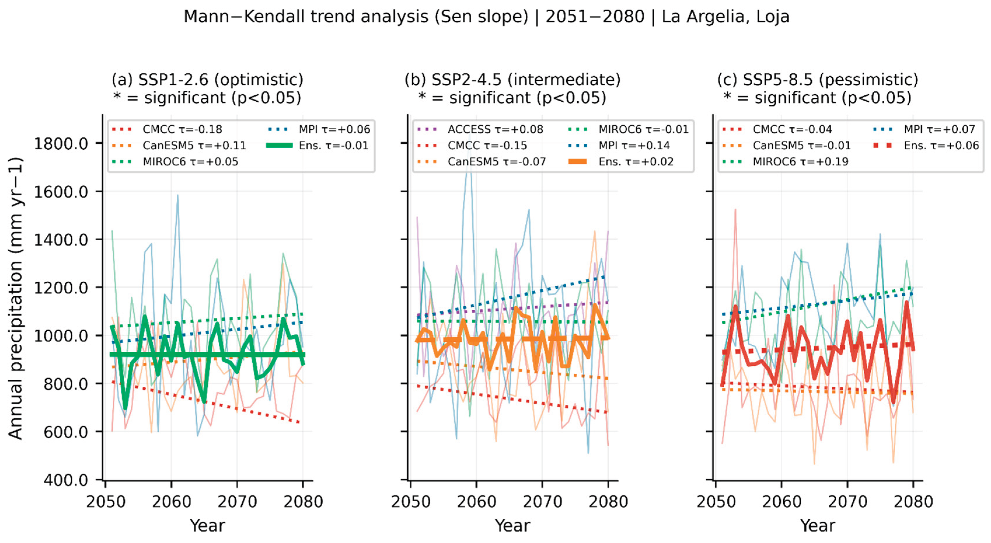
Figure 11.
Monthly uncertainty decomposition and annual scenario spread. (a) Monthly variance partitioning into scenario, model, and model × scenario interaction components. (b) Annual precipitation totals per scenario (box = interquartile range [IQR]; whiskers = 5th–95th percentile; dashed line = observed mean of 933 mm year⁻¹).
Figure 11.
Monthly uncertainty decomposition and annual scenario spread. (a) Monthly variance partitioning into scenario, model, and model × scenario interaction components. (b) Annual precipitation totals per scenario (box = interquartile range [IQR]; whiskers = 5th–95th percentile; dashed line = observed mean of 933 mm year⁻¹).
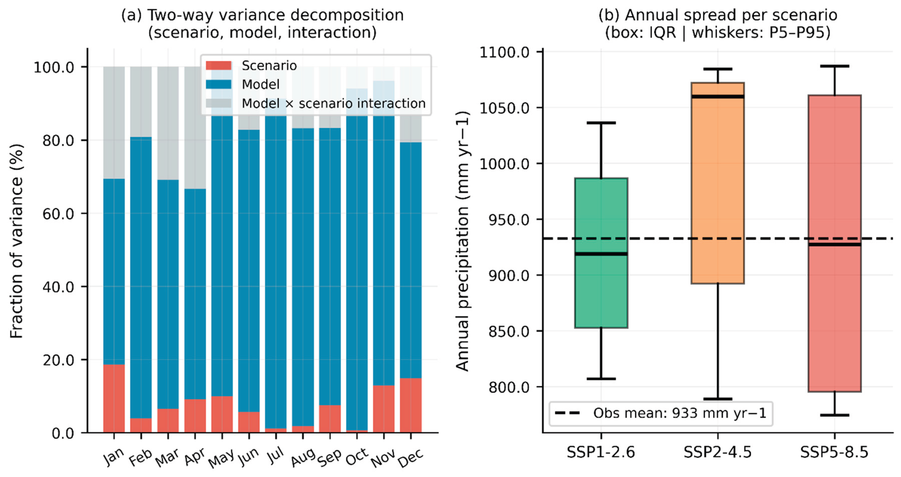
Figure 12.
Signal-to-Noise (S/N) ratio and inter-model consensus on the direction of monthly precipitation change. (a) Monthly S/N ratio for each SSP scenario, dashed line at the robustness threshold (S/N = 1.0). (b) Percentage of models agreeing on the sign of the monthly precipitation anomaly, dashed line at the 80% agreement threshold.
Figure 12.
Signal-to-Noise (S/N) ratio and inter-model consensus on the direction of monthly precipitation change. (a) Monthly S/N ratio for each SSP scenario, dashed line at the robustness threshold (S/N = 1.0). (b) Percentage of models agreeing on the sign of the monthly precipitation anomaly, dashed line at the 80% agreement threshold.
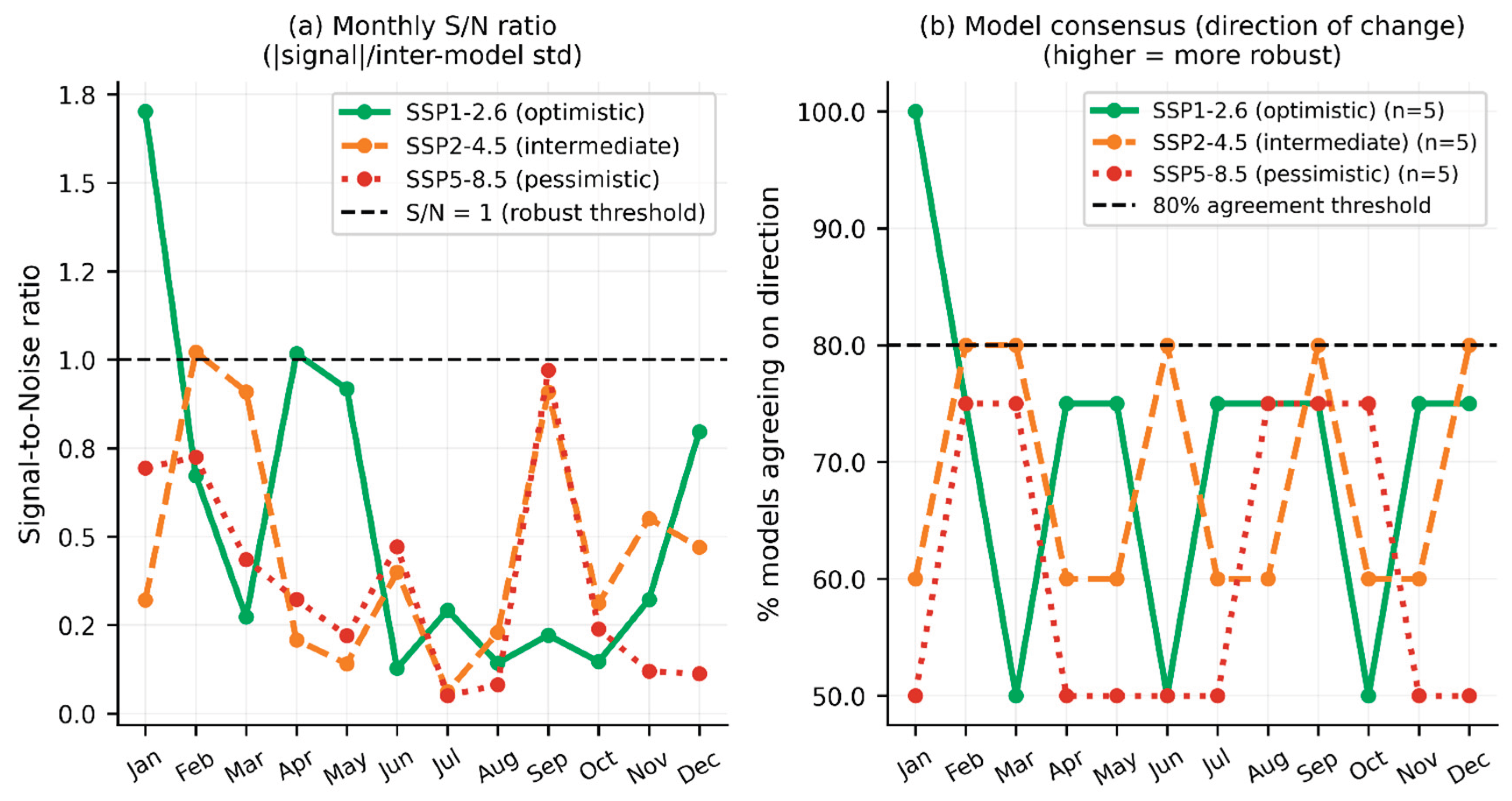
Figure 13.
Robust change summary matrix. Ensemble-mean monthly precipitation change (mm month⁻¹) for 2051–2080 relative to the 1981–2010 across the three SSP scenarios; checkmarks (✓) denote a robust signal where at least 80% of the available models agree on the sign of change.
Figure 13.
Robust change summary matrix. Ensemble-mean monthly precipitation change (mm month⁻¹) for 2051–2080 relative to the 1981–2010 across the three SSP scenarios; checkmarks (✓) denote a robust signal where at least 80% of the available models agree on the sign of change.
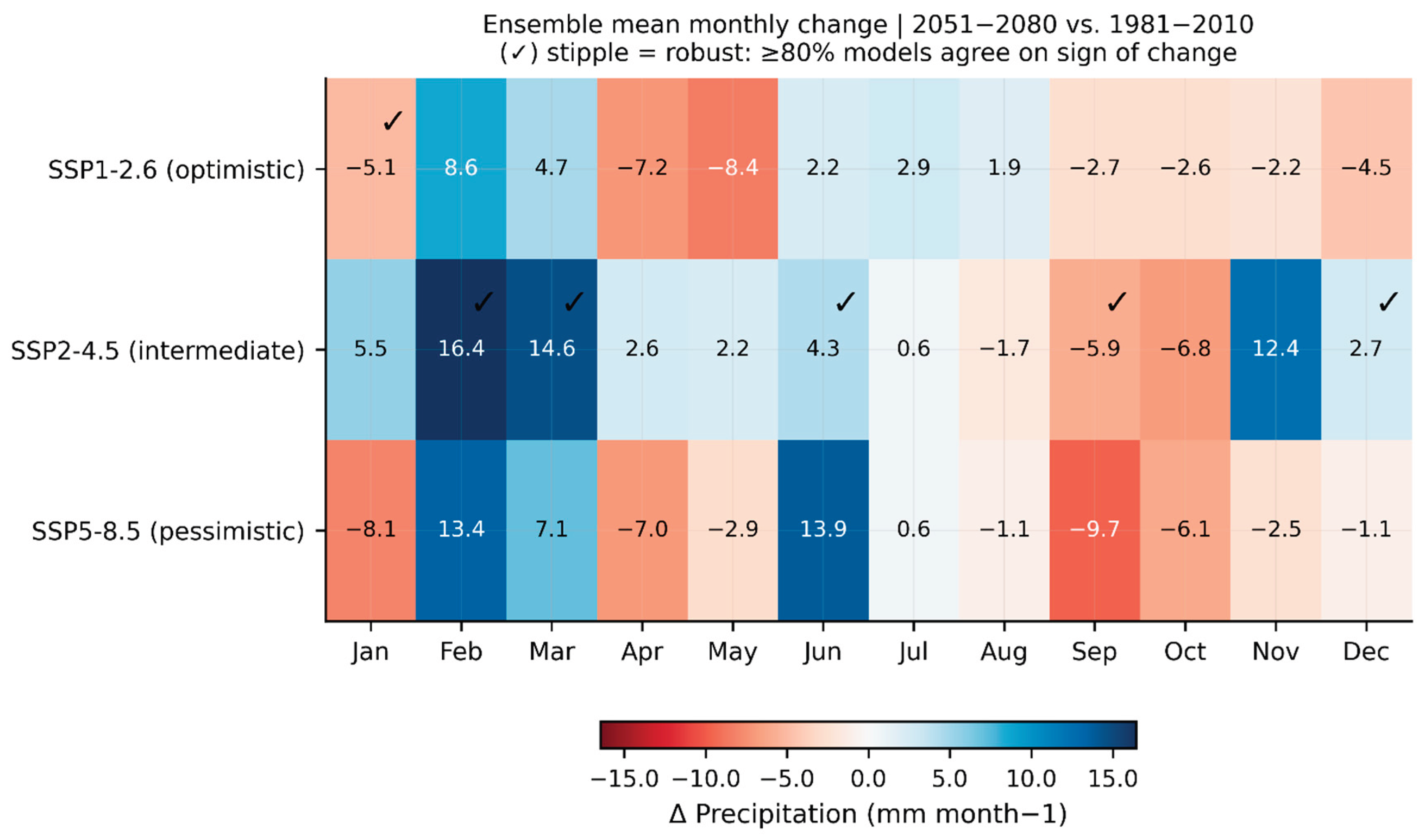
Figure 14.
Taylor diagrams summarizing multi-metric GCM fidelity against SC-PREC4SA observations: (a) historical raw GCMs (1981–2010) and (b) the downscaled SSP2-4.5 future ensemble (2051–2080).
Figure 14.
Taylor diagrams summarizing multi-metric GCM fidelity against SC-PREC4SA observations: (a) historical raw GCMs (1981–2010) and (b) the downscaled SSP2-4.5 future ensemble (2051–2080).
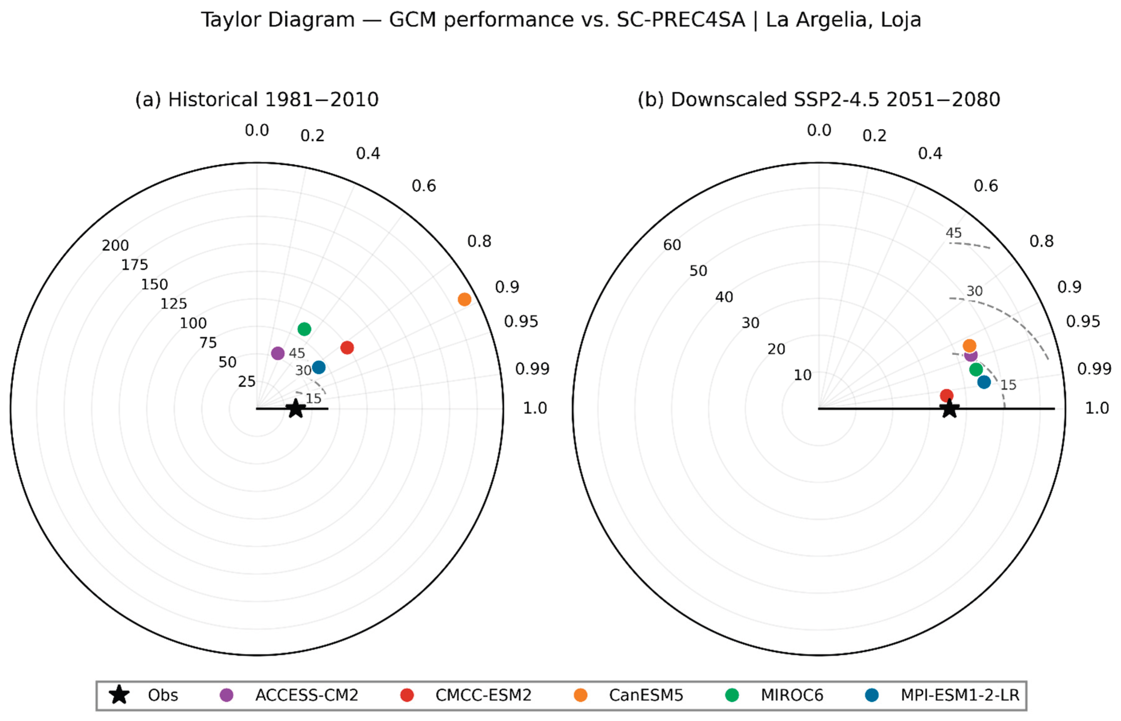
Figure 15.
Multi-metric radar chart and composite GCM ranking. (a) Normalized scores (Pearson r, KGE, NSE, and inverted RMSE and Bias) for all five CMIP6 models. (b) Composite ranking (mean of the normalized metrics).
Figure 15.
Multi-metric radar chart and composite GCM ranking. (a) Normalized scores (Pearson r, KGE, NSE, and inverted RMSE and Bias) for all five CMIP6 models. (b) Composite ranking (mean of the normalized metrics).
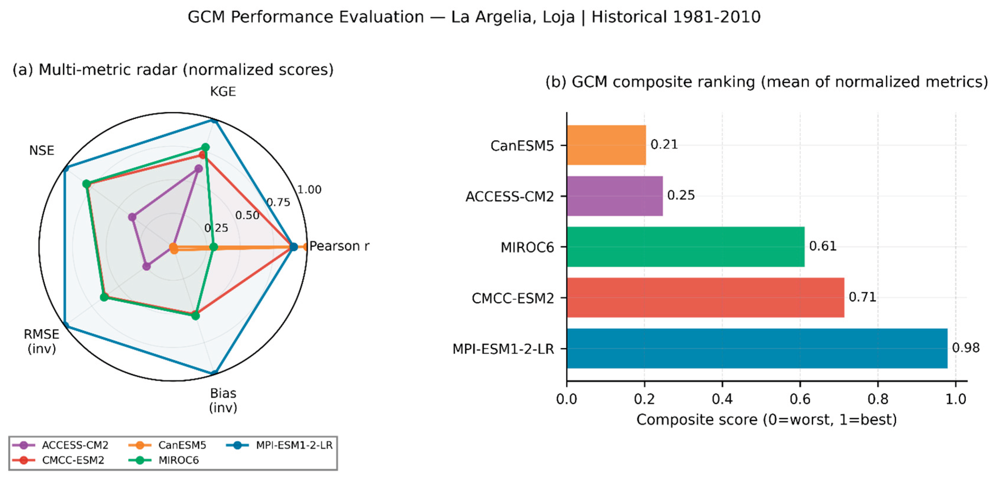
Figure 16.
Seasonal precipitation disaggregation under three SSP scenarios (2051–2080 vs. 1981–2010): (a) DJF, (b) MAM, (c) JJA, and (d) SON.
Figure 16.
Seasonal precipitation disaggregation under three SSP scenarios (2051–2080 vs. 1981–2010): (a) DJF, (b) MAM, (c) JJA, and (d) SON.
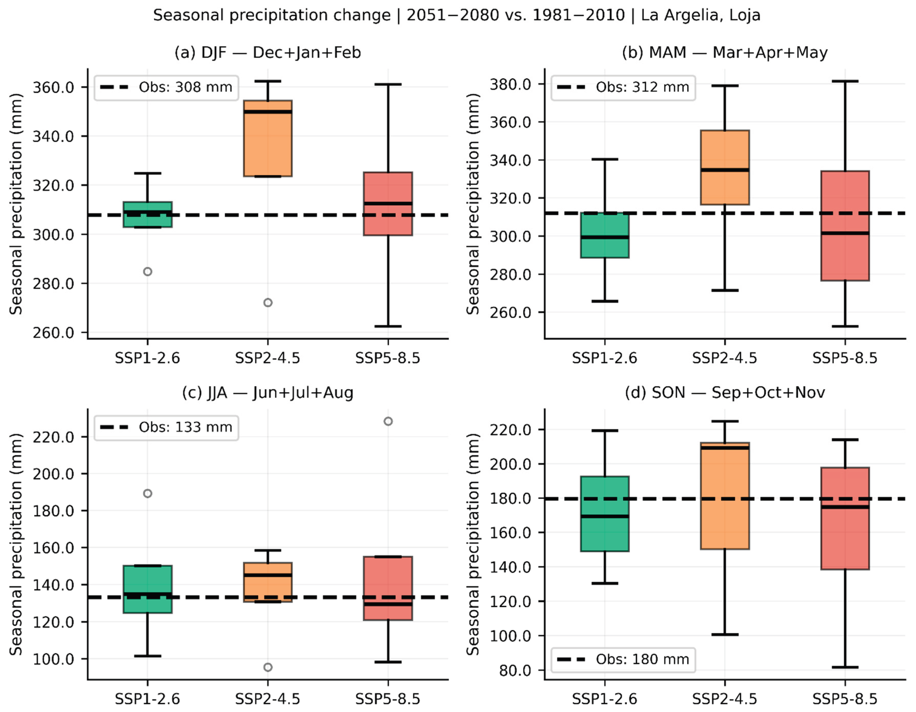
Figure 17.
Dry- and wet-spell duration statistics (mean and 90th percentile) for 2051–2080 relative to the observed baseline (1981–2010).
Figure 17.
Dry- and wet-spell duration statistics (mean and 90th percentile) for 2051–2080 relative to the observed baseline (1981–2010).
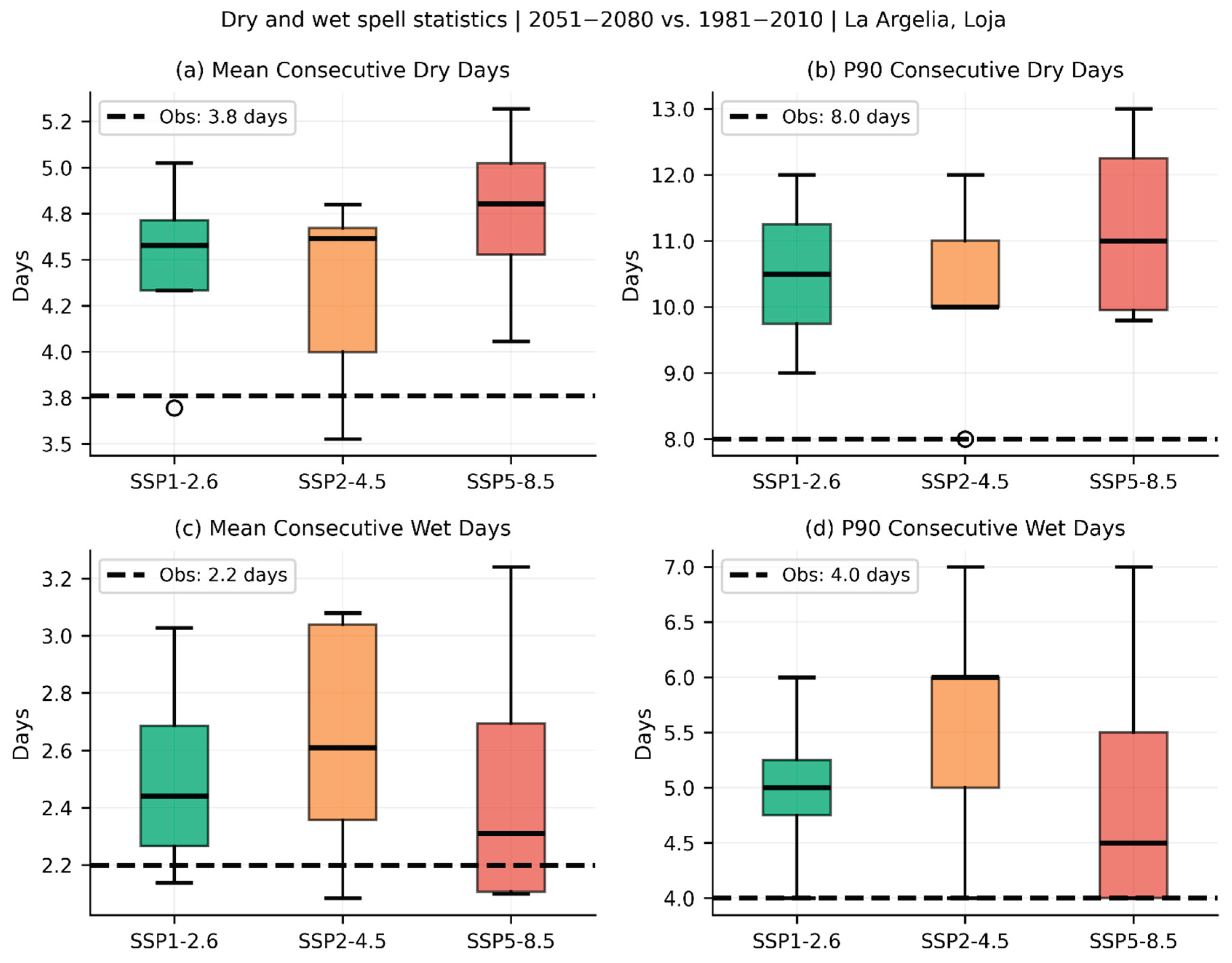
Figure 18.
Precipitation change disaggregated by intensity percentile bins (P0–20 to P95–100), by scenario: (a) SSP1-2.6, (b) SSP2-4.5, and (c) SSP5-8.5. Bottom row (ENS) is the ensemble mean.
Figure 18.
Precipitation change disaggregated by intensity percentile bins (P0–20 to P95–100), by scenario: (a) SSP1-2.6, (b) SSP2-4.5, and (c) SSP5-8.5. Bottom row (ENS) is the ensemble mean.
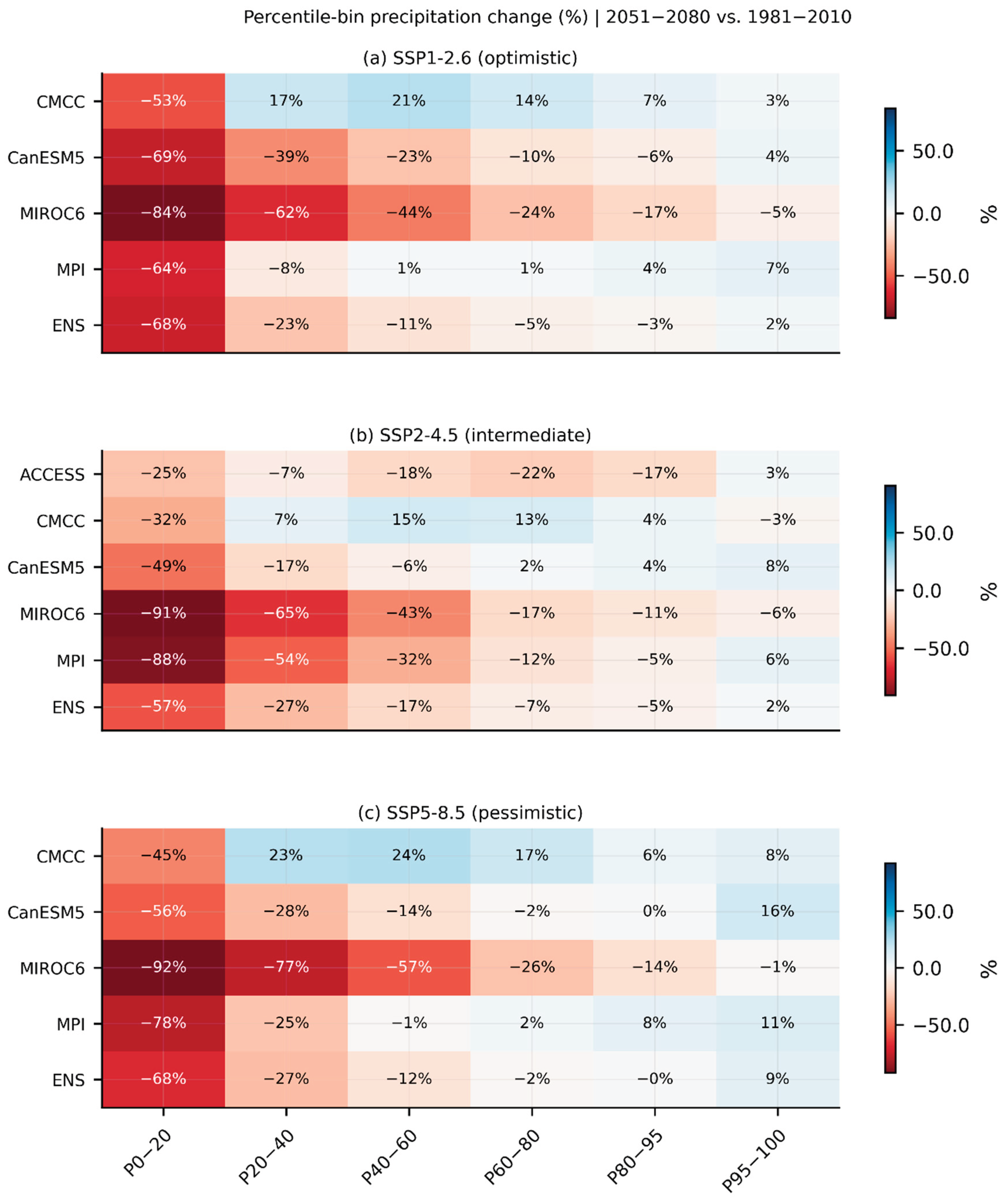
Figure 19.
Probability of exceedance for daily precipitation thresholds of 10, 20, 30, and 50 mm day⁻¹. (a) Exceedance frequency by scenario. (b) Absolute change in exceedance frequency (percentage points) relative to the observed baseline.
Figure 19.
Probability of exceedance for daily precipitation thresholds of 10, 20, 30, and 50 mm day⁻¹. (a) Exceedance frequency by scenario. (b) Absolute change in exceedance frequency (percentage points) relative to the observed baseline.
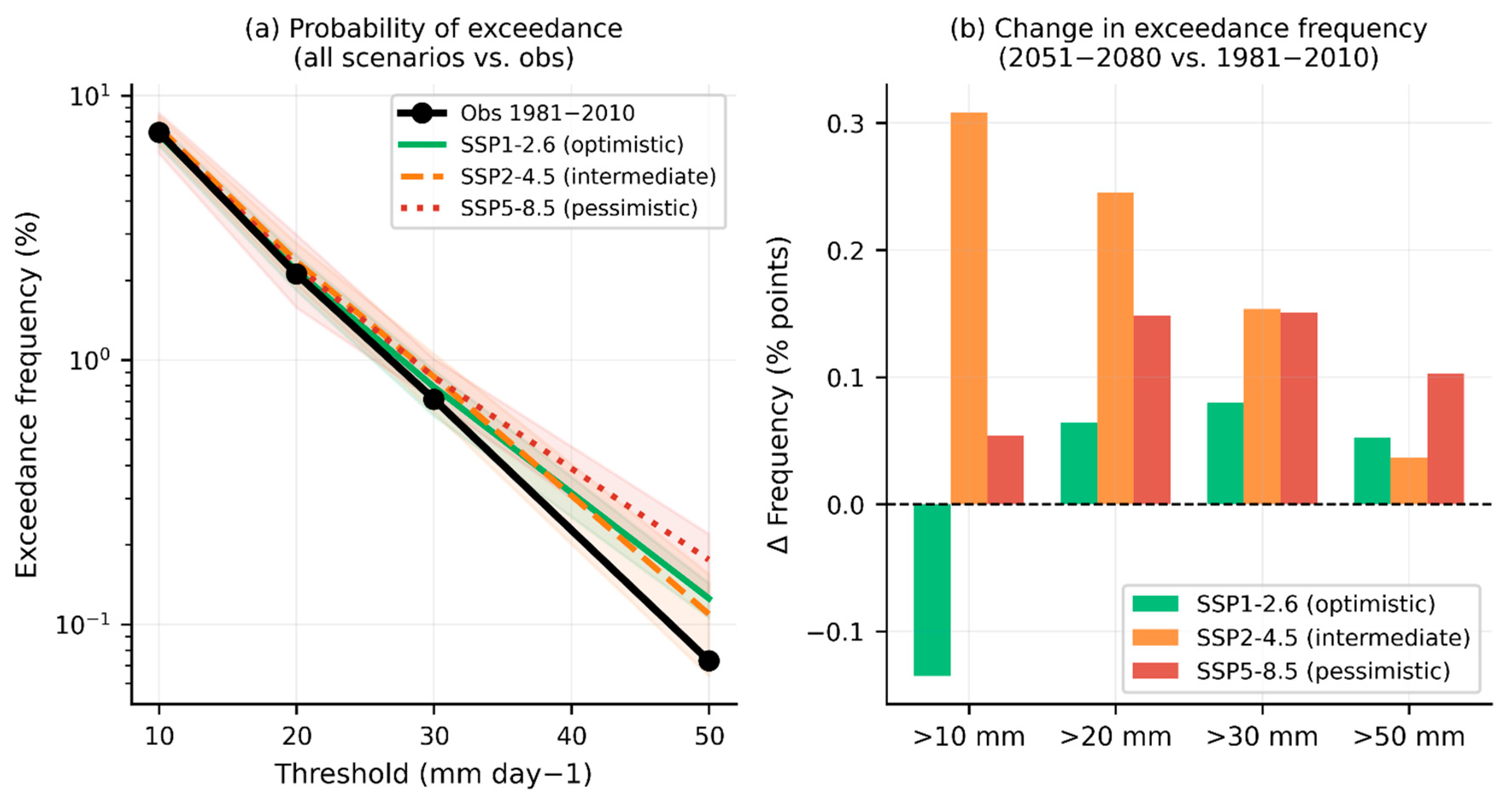
Figure 20.
Comprehensive precipitation statistics summary table across all scenario–model combinations, including annual totals, spell statistics, 1-day maxima, and 50-year return levels.
Figure 20.
Comprehensive precipitation statistics summary table across all scenario–model combinations, including annual totals, spell statistics, 1-day maxima, and 50-year return levels.
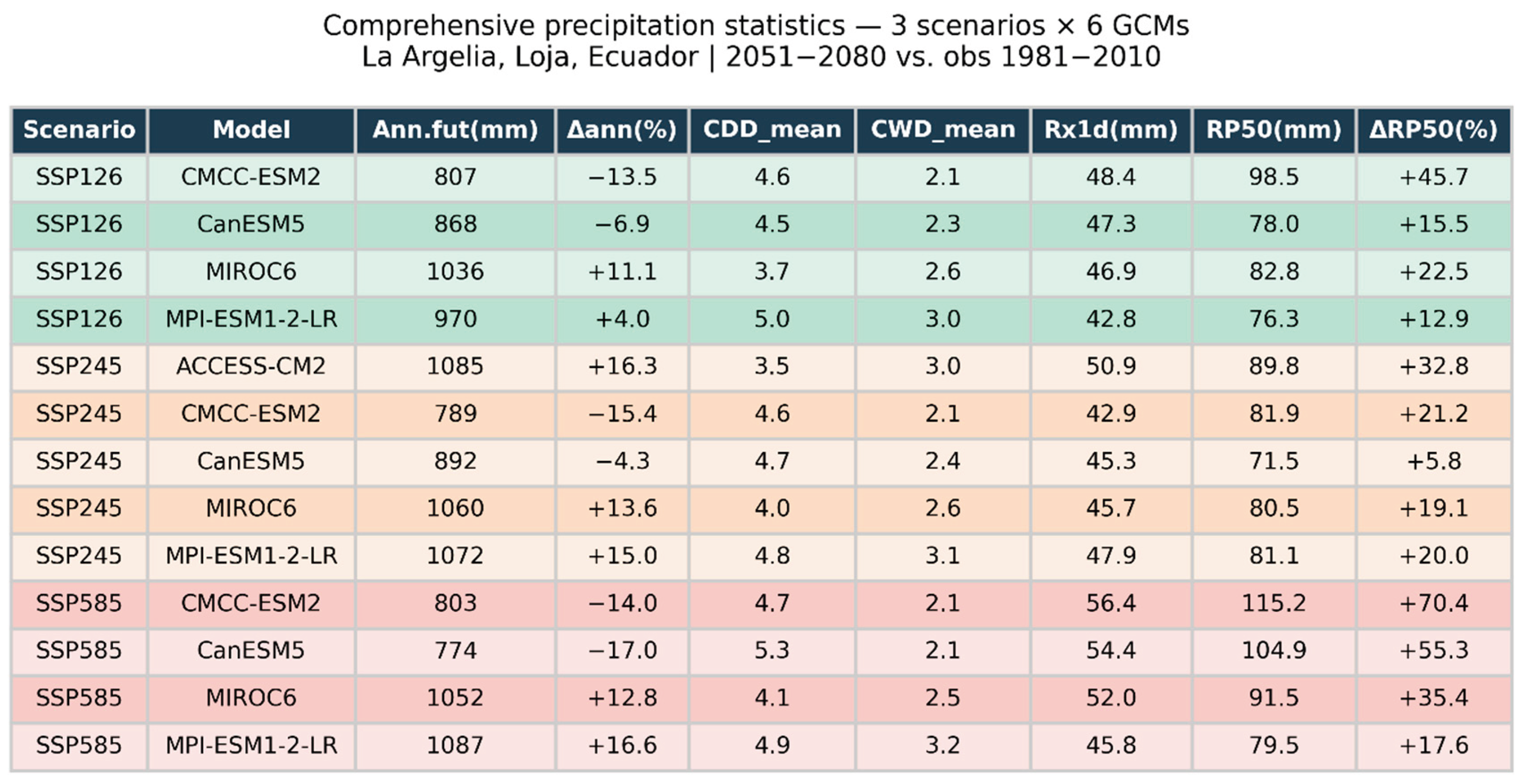

Table 1.
Definition, units, and mathematical formulation of the extreme precipitation indices computed in this study.
Table 1.
Definition, units, and mathematical formulation of the extreme precipitation indices computed in this study.
| Acronym | Definition | Units | Equation | Eq. No. |
| Rx1day | Maximum 1-day precipitation amount | mm | (5) | |
| Rx5day | Maximum 5-day consecutive precipitation amount | mm | (6) | |
| SDII | Simple Precipitation Intensity Index (mean precipitation on wet days) | mm day⁻¹ | (7) | |
| R95p | Total annual precipitation from days exceeding the 95th percentile | mm | (8) | |
| CWD | Maximum number of consecutive wet days | days | (9) | |
| CDD | Maximum number of consecutive dry days | days | (10) |
Where Rij is the precipitation amount on day j in year i; J is the number of wet days (where Rij≥1 mm); R95 is the 95th percentile of daily precipitation; and Lw and Ld are the lengths of consecutive wet and dry sequences, respectively.
Table 2.
GCM performance evaluation metrics against SC-PREC4SA observations at La Argelia station (1981–2010). Bold: best-performing model. WF_err = wet-day frequency error relative to observed 36.8%; P95_ratio = ratio of modelled to observed 95th-percentile daily precipitation.
Table 2.
GCM performance evaluation metrics against SC-PREC4SA observations at La Argelia station (1981–2010). Bold: best-performing model. WF_err = wet-day frequency error relative to observed 36.8%; P95_ratio = ratio of modelled to observed 95th-percentile daily precipitation.
| Model | r | Bias(%) | RMSE | MAE | NSE | KGE | PBIAS(%) | WF_err(%) | P95_ratio | Rank |
| MPI-ESM1-2-LR | 0.830 | 23.630 | 45.147 | 35.060 | –0.776 | 0.042 | 23.63 | 14.867 | 0.717 | 1 |
| MIROC6 | 0.511 | 133.937 | 125.295 | 105.674 | –12.683 | –0.985 | 133.937 | 17.131 | 1.613 | 2 |
| CMCC-ESM2 | 0.828 | 136.627 | 126.864 | 106.188 | –13.027 | –1.265 | 136.627 | 50.051 | 0.945 | 3 |
| CanESM5 | 0.884 | 257.851 | 265.888 | 209.341 | –60.617 | –4.647 | 257.851 | 27.101 | 2.336 | 4 |
| ACCESS-CM2 | 0.350 | 263.997 | 211.409 | 205.180 | –37.954 | –1.769 | 263.997 | 50.954 | 1.428 | 5 |
Table 3.
Independent split-sample validation: raw and bias-corrected skill metrics for 2001–2010, calibrated using only 1981–2000.
Table 3.
Independent split-sample validation: raw and bias-corrected skill metrics for 2001–2010, calibrated using only 1981–2000.
| Model | NSE_raw | NSE_corrected | KGE_raw | KGE_corrected | PBIAS_raw(%) | PBIAS_corrected(%) |
| ACCESS-CM2 | −47.59 | 0.68 | −1.88 | 0.74 | 265.4 | 10.5 |
| CMCC-ESM2 | −16.78 | 0.58 | −1.62 | 0.60 | 132.4 | −1.7 |
| CanESM5 | −71.72 | 0.45 | −5.04 | 0.66 | 249.9 | −3.2 |
| MIROC6 | −15.55 | 0.56 | −1.24 | 0.66 | 127.7 | −3.1 |
| MPI-ESM1-2-LR | −1.20 | 0.58 | −0.08 | 0.76 | 18.0 | −6.0 |
Table 4.
Annual precipitation summary for ensemble mean under three SSP scenarios (2051–2080) versus the observed baseline (1981–2010). The range spans the 10th–90th percentile of each model's own mean annual total.
Table 4.
Annual precipitation summary for ensemble mean under three SSP scenarios (2051–2080) versus the observed baseline (1981–2010). The range spans the 10th–90th percentile of each model's own mean annual total.
| Scenario | Obs (mm yr⁻¹) |
Future Ens. (mm yr⁻¹) |
Δ (mm yr⁻¹) |
Δ (%) |
P10 (mm yr⁻¹) |
P90 (mm yr⁻¹) |
| SSP1-2.6 (optimistic) | 932.6 | 920.6 | −12.1 | −1.3 | 825 | 1016 |
| SSP2-4.5 (intermediate) | 932.6 | 979.9 | +47.2 | +5.1 | 830 | 1080 |
| SSP5-8.5 (pessimistic) | 932.6 | 929.4 | −3.3 | −0.4 | 783 | 1077 |
Table 5.
ETCCDI extreme precipitation indices: observed baseline (1981–2010) and ensemble mean (± inter-model standard deviation) for 2051–2080 under three SSP scenarios.
Table 5.
ETCCDI extreme precipitation indices: observed baseline (1981–2010) and ensemble mean (± inter-model standard deviation) for 2051–2080 under three SSP scenarios.
| Index (units) | Observed | SSP1-2.6 (mean ± σ) |
SSP2-4.5 (mean ± σ) |
SSP5-8.5 (mean ± σ) |
| Rx1day (mm) | 40.5 | 46.4 ± 1.3 | 46.6 ± 1.9 | 52.2 ± 2.6 |
| Rx5day (mm) | 80.3 | 88.5 ± 2.1 | 92.7 ± 4.4 | 91.9 ± 1.9 |
| SDII (mm day⁻¹) | 6.70 | 6.7 ± 0.1 | 6.8 ± 0.1 | 7.3 ± 0.1 |
| R95p (mm) | 399 | 407 ± 14 | 417 ± 15 | 421 ± 20 |
| CWD (days) | 8.7 | 11.2 ± 1.7 | 13.7 ± 2.2 | 11.6 ± 2.8 |
| CDD (days) | 19.5 | 28.6 ± 2.1 | 26.8 ± 3.3 | 29.3 ± 3.1 |
Table 6.
Gumbel maximum-likelihood return levels (mm day⁻¹) at La Argelia station. Bootstrap 95% confidence intervals in brackets.
Table 6.
Gumbel maximum-likelihood return levels (mm day⁻¹) at La Argelia station. Bootstrap 95% confidence intervals in brackets.
| Scenario | n | RP-10 (mm) |
RP-50 (mm) |
RP-100 (mm) |
| Observed (1981–2010) | — | 54.2 [CI: 47.7–59.7] | 67.6 [CI: 58.1–75.4] | ~73.2 |
| SSP1-2.6 | 4 | 65.1 ± 5.1 | 83.9 ± 8.7 | 91.9 ± 10.3 |
| SSP2-4.5 | 5 | 63.7 ± 3.9 | 80.9 ± 5.8 | 88.3 ± 6.7 |
| SSP5-8.5 | 4 | 74.9 ± 8.4 | 97.8 ± 13.5 | 107.5 ± 15.7 |
Disclaimer/Publisher’s Note: The statements, opinions and data contained in all publications are solely those of the individual author(s) and contributor(s) and not of MDPI and/or the editor(s). MDPI and/or the editor(s) disclaim responsibility for any injury to people or property resulting from any ideas, methods, instructions or products referred to in the content. |
© 2026 by the authors. Licensee MDPI, Basel, Switzerland. This article is an open access article distributed under the terms and conditions of the Creative Commons Attribution (CC BY) license (http://creativecommons.org/licenses/by/4.0/).
Copyright: This open access article is published under a Creative Commons CC BY 4.0 license, which permit the free download, distribution, and reuse, provided that the author and preprint are cited in any reuse.


