

Submitted:
09 August 2026
Posted:
10 August 2026
You are already at the latest version
Abstract
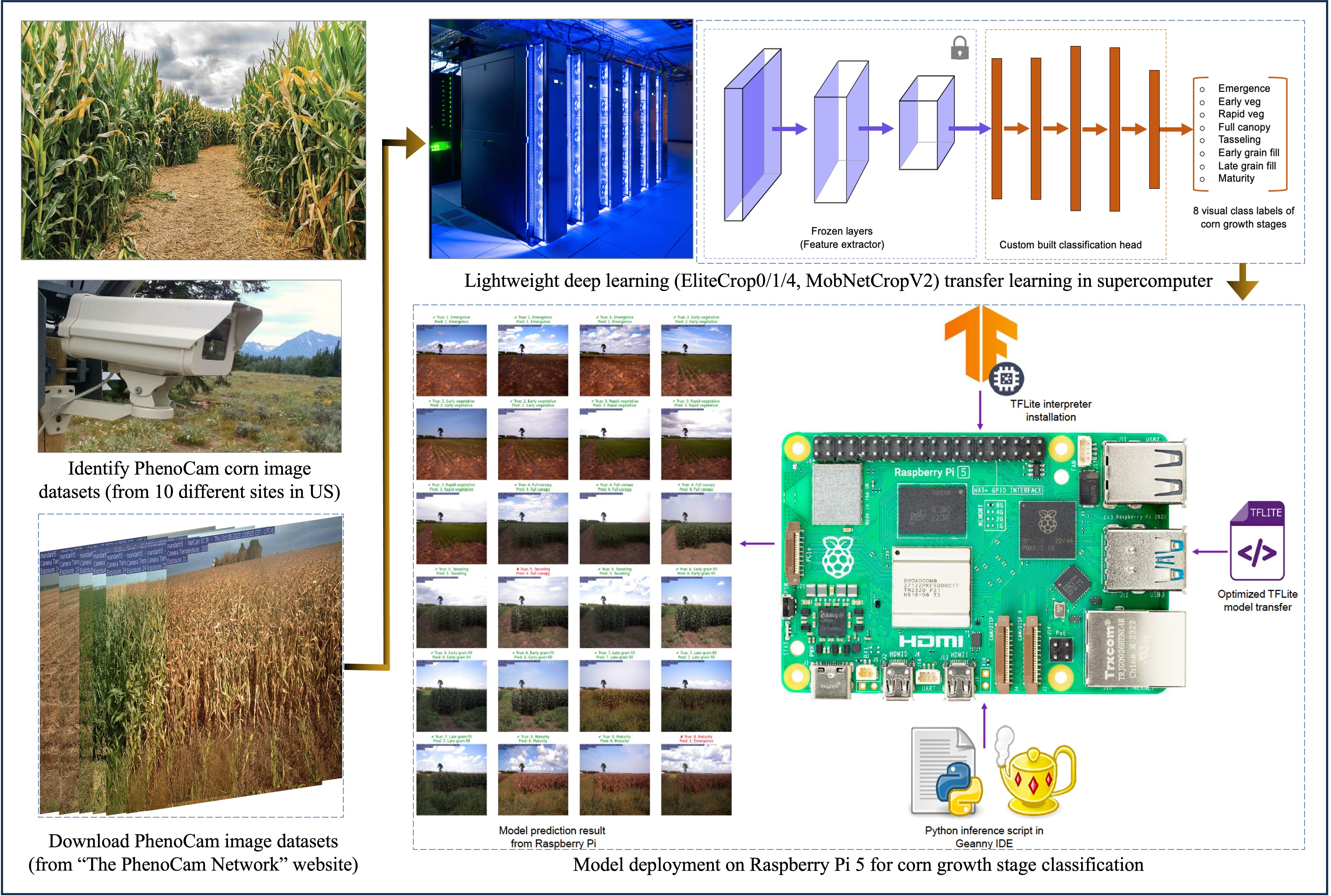
Integrating precision agriculture (PA, a data-driven agricultural management system) with deep learning (DL) models can effectively support various activities, including yield prediction, crop health monitoring, field task automation, and decision-making. Taking advantage of such data-driven methodologies typically requires desktops, high-performance computing systems, and cloud clusters for data analysis, but their portability limits in-field applications. However, a single board computer, such as Raspberry Pi, offers a compact, lightweight, cost-efficient, easy-to-use, and feature-rich portable computing device which is ideal for in-field decision-making in PA applications. One such in-field application is crop growth stage classification for better crop management. Therefore, in this study, eight corn growth stages were classified using PhenoCam (near-surface [proximal] remote sensing network camera)imagery collected from ten PhenoCam sites. Four lightweight DL models were developed, ELiteCrop0, ELiteCrop1, ELiteCrop4, and MobNetCropV2, and evaluated across five image vertical clipping levels(0 %–40 %) using a supercomputer. The optimized model was subsequently deployed on a Raspberry Pi5 for edge inference. Model training accounted for the majority of the total CPU time, exceeding 97 %, while the testing times ranged from 0.01 min to 0.12 min, enabling real-time applications. Among the models, ELiteCrop0 achieved the most balanced performance with a confusion-matrix diagonal ratio(CMDR) of 0.93, followed by ELiteCrop1 (CMDR = 0.92). Overall, model performance decreased with increasing vertical clipping; therefore, a moderate image clipping (0 %–10 %) was recommended for improved computational efficiency. Analysis with a supercomputer produced an intrasite (same train sites)accuracy of 0.90–0.93 (Raspberry Pi: 0.78–0.81) and an intersite (new test sites) accuracy of 0.48–0.50(Raspberry Pi: 0.41–0.43), indicating challenges with model generalization. Raspberry Pi successfully processed ≈ 1000 images/min under safe operating conditions (68◦C). Future work should focus on extending the multi-site dataset to improve cross-site performance. Hence, this study presents a scalable and cost-effective solution for real-time corn growth stage monitoring in PA.
Keywords:
data-driven agriculture
; deep learning
; lightweight model
; PhenoCam
; precision agriculture
; Raspberry Pi
1. Introduction
Agricultural crop growth monitoring is the method of systematically observing and analyzing the overall health of crops throughout their life cycle. This process involves regular and frequent inspections of crops to collect data on their health, development stages, and maturity (Sreekantha and Kavya, 05-06 January 2017). Different crops require different environmental conditions, such as soil moisture, temperature, humidity, nutrient levels, and light intensity, depending on their growth phases. To optimize crop yield and determine the optimal harvest time for maximum profitability, it is essential to understand the timing of nutrient application and the management of environmental factors at each growth stage. For instance, nitrogen side-dress applications are most effective between V4 and V6 (late stages of “early vegetative” assigned class label #2 in this study; Section 2.2) before peak nutrient demand; post-emergent herbicides carry strict application cutoffs typically at V6 or earlier depending on the herbicide application. While accurate identification of late reproductive stages such as R4 and R5 (end stages of “early grain fill” to “late grain fill” assigned class labels #6 and #7 in this study; Section 2.2) enables reliable harvest timing and logistics planning, especially in short growing seasons, such that misidentifying a growth stage transition, even by a few days, can cascade into suboptimal input timing and measurable yield losses (Soltani et al., 2022). Corn, despite its determinate growth pattern, presents unique challenges in identifying its growth stages due to its heightened sensitivity to stress during critical reproductive stages (cfa). This knowledge also facilitates decision-making related to pesticide and herbicide application and contributes to selective breeding efforts (Jeong and Lee, 29 November - 02 December 2022). Hence, this research focuses on classifying the growth stages of corn using efficient real-time monitoring methods.
Some of the conventional challenges faced during monitoring crops for classifying their growth stages are labor-intensive field scouting, inadequate temporal and spatial resolution, subjective assessment, and delayed detection of crop stress and disease. These challenges often lead to inefficient monitoring, resulting in poor management practices (Rasti et al., 2021). In order to address some of the conventional challenges, precision agriculture (PA) enhances agricultural crop growth monitoring through the utilization of advanced tools and technologies.
The application of advanced PA technologies include global positioning system (GPS), sensors, remote sensing, computer vision (CV), robotics, satellites, unmanned aerial vehicles (UAVs), PhenoCam, and artificial intelligence (AI) for data-driven decision-making. These approaches help to monitor crops effectively, make informed decisions, optimize inputs, improve yield and productivity, enhance resource management, and minimize environmental impacts (Shafi et al., 2019).
As PA tools continue to evolve, the importance of real-time, continuous, and accurate monitoring of crop growth becomes more essential. One of the most effective near-surface (proximal) remote sensing techniques used in PA for monitoring crops at various growth stages is PhenoCam (Yu et al., 2024). PhenoCam is a digital camera that captures time-lapse images of vegetation cover and helps to observe changes in specific geo-location ecosystems over time (Richardson, 2023; Sunoj et al., 2025). The “PhenoCam Network" is a cooperative, continental-scale monitoring network hub that employs digital cameras to collect imagery for tracking vegetation phenology (phe), supports long-term ecological monitoring from various sites, and the infrastructure is managed by Northern Arizona University (Richardson, 2023). Based on their adherence to the network’s standard protocol, the degree of on-site personnel collaboration, and image quality, PhenoCam network sites are classified as Type I (highest), II, and III (lowest). As of May 2026, the types (number of sites) displayed in the network are: Type I (911), Type II (106), and Type III (39); out of which 195 are agricultural sites (https://phenocam.nau.edu/webcam/gallery/). Using color vegetation indices (CVI) extracted from PhenoCam images and relating CVI curves, phenological growth stages are estimated (Liu et al., 2022; Toda and Richardson, 2018).
In PA, AI methodologies provide more informed decisions for monitoring crops, identifying pests, managing nutrients, planting seeds, and detecting weeds. With recent applications of deep neural computing algorithms in PA, deep learning (DL; a subset of AI) models learn features automatically from raw data, thereby eliminating the need to manually extract features from the data (Chettri et al., 2026). An important capability of DL models is their ability to modify and improve performance dynamically (Shah et al., 2023). However, DL models require voluminous data inputs, high computational loads, and time delay in post-data processing; therefore, there exists a need for efficient and timely decision-making techniques. PhenoCam image-based DL classification has been primarily used for weed and crop disease detection (Jha et al.; Benos et al., 2021), and monitoring daily crop phenology (Taylor and Browning, 2022). Recent studies demonstrate that phenological characteristics obtained from PhenoCam images enable high-throughput plant phenotyping to track crop traits (Jin et al., 2020; Guo, 2025).
In order to make timely interventions, make infield decisions, address limited resources, overcome data-related challenges, and reduce computational loads, lightweight DL models (less memory, lower computational power, fewer parameters than conventional DL models, and deployable in smaller edge devices) are essential for practical deployment in PA. Lightweight DL focused on prioritizing efficiency, increasing inference speed, reducing power consumption, and compactness, especially made for embedded applications. These lightweight DL models have the ability to precisely identify and separate the essential features automatically using dimensionality reduction (Sharma et al., 2022). Some of the commonly used lightweight DL models in PA applications are MobileNet, EfficientNet-Lite, Tiny-YOLO, YOLO-Nano, and SqueezeNet (Albahli, 2025; Kolhe et al., 11-13 June 2025; Lu et al., 2023; Qin et al., 2021; Abo Khalaf, 2024).
To enable real-time infield analysis and faster decision-making in PA, lightweight DL models are deployed using edge computing. Edge computing refers to processing data locally near the point of collection rather than transferring it to remote locations or cloud servers. Some of the deployment techniques, such as transfer learning, model quantization, pruning, and knowledge distillation, further enable efficient deployment on resource-constrained devices. Single board computers (SBCs), also called edge devices, are portable computing devices specially designed for performing edge computing tasks. These devices are compact, portable, and easy-to-use, equipped with a microprocessor, memory, input/output connections, and Ethernet. Some of the available SBCs include Arduino UNO, BeagleBone, Intel Galileo, LattePanda, Odroid, Odyssey, Nvidia Jetson, Tinker Board, and Raspberry Pi. They are widely used for monitoring, industrial automation, prototyping, robotics, and embedded applications (Joice et al., 2025). Among SBCs, Nvidia Jetson and Raspberry Pi are commonly employed for deploying lightweight DL models (Liu et al., 2024). Due to their cost-effectiveness, versatility, low power consumption, built-in wireless connectivity, low latency, energy efficiency, complex computational capability, and real-time applicability, Raspberry Pi was selected to deploy a lightweight DL model for this study. Additionally, the transfer learning technique was used to shorten training times and improve model performance so that the final lightweight model could function effectively on Raspberry Pi.
The hypothesis of this study is that lightweight DL models can be effectively deployed on edge devices such as Raspberry Pi to classify corn growth stages, providing a scalable and cost-efficient solution for agricultural monitoring. The overall objective is to design, deploy, and evaluate lightweight DL models for corn growth stage classification on the Raspberry Pi.
The specific objectives of this research are to: (i) design and develop lightweight DL model using transfer learning technique on North Dakota State University’s (NDSU) Center for Computationally Assisted Science and Technology (CCAST) supercomputer; (ii) analyze the impact of image preprocessing technique, namely vertical clipping (0%–40%), on model learning, classification performance, and computational efficiency; (iii) assess lightweight DL model performance using classification metrics and confusion matrix analysis (intrasite); (iv) evaluate model’s generalization using new PhenoCam sites as test dataset (intersite); (v) deploy the model on Raspberry Pi 5 and evaluate its real-time inference capability; and (vi) comparison of model performance with respect to CCAST supercomputer and Raspberry Pi.
2. Materials and Methods
The overall flow chart showing the research work of this study and the work plan performed for this research is shown in Figure 1.
2.1. Description of Data Source and Study Sites
PhenoCams were installed in the USA as part of the NEON (National Ecological Observatory Network) and LTAR (Long Term Agricultural Research) networks to capture high-frequency RGB imagery that helps in monitoring seasonal vegetation dynamics. The captured images along with their phenological metrics are stored in the dataset, which is publicly available (https://phenocam.nau.edu/). For the study, PhenoCam images were collected from ten different PhenoCam sites that are planted with corn across different states in the US for the years spanning 2023–2025.
The first five PhenoCam sites were selected for the intrasite (training and testing within sites; only for 2023) approach. Some of the main considerations for choosing these five PhenoCam sites for our study (intrasite) are: Consistent crop type and year—the availability of corn-planted sites in 2023 due to annual crop rotation between corn and soybean, control of inter-annual variability, and for better comparison of growing season; Geographical diversity—these sites are from multiple states, representing different climatic zones and agronomic conditions; and Alignment with the US agricultural trends—they are located in major corn-growing regions of the US.
The next five PhenoCam sites were used for intersite (new test sites; 2024 & 2025). The considerations for selecting the intersites are: (i) corn planted sites on a later date (2024 & 2025) can be predicted from the previous year (2023) data, and (ii) geographical diversity. Table 1 presents details about environmental and geographical characteristics of the selected individual sites (Figure 2).
2.2. Data Acquisition and Visual Class Labeling
PhenoCam images from selected corn-planted study sites were downloaded from the PhenoCam Network (https://phenocam.nau.edu/webcam/network/download/, accessed on 29 June 2026). The specific inputs provided were the site name, start and end dates, and start and end times of a day. Images were collected as individual folders from May to October for a widely recommended time range between 10:00 h and 14:00 h (Meng et al., 2024; Songsom et al., 2021). Raw images were downloaded in JPEG format at their inherent resolution (1296 960 px). The downloaded PhenoCam dataset consists of automatically split individual subfolders by month (May to October (6): ‘5’–‘10’), corresponding to the input date range.
In general, the entire life cycle of the corn plant is broadly classified into two stages: vegetative (V) and reproductive (R). The vegetative growth stage consists of VE (emergence), V1, V2, V3, and so on, up to V(n), where n denotes the last stage of the vegetative phase before the initiation of the reproductive phase, and VT (tassel). The reproductive growth stages include R1 (silk), R2 (blister), R3 (milk), R4 (dough), R5 (dent), and R6 (physiological maturity) (plu). However, in this study, the above-mentioned conventional agronomic corn growth stages were not considered in the DL model development for classification using PhenoCam images.
For DL model development, PhenoCam images need to be manually classified and labeled into the various growth stages of interest. For the manual classification, visual appearance cues such as canopy structure, color variation, and reproductive features in the PhenoCam imagery were utilized (Bloomfield et al., 2014; Badu-Apraku and Fakorede, 2017). The eight generated class labels and visual appearance verbal descriptions are presented in Table 2, while the diagrammatic description classes with corresponding samples of PhenoCam images are presented in Figure 3.
Based on visual appearance cues (Table 2 and Figure 3), the PhenoCam images were manually classified and stored in the appropriately “labelled folders” following the aforementioned eight class labels. Following the time duration of the crop growth cycle, the number of images under each stage in these folders will be imbalanced and needs to be addressed, which is subsequently handled using stratified data splitting (Section 2.3.2).
2.3. Google Colab and CCAST Supercomputer for Training
To process and analyze PhenoCam images found inside the annotated folders, we initially used Google Colab, a cloud-based IDE (integrated development environment) with several pre-installed features for model development built on Jupyter Notebook. The training time for each model was approximately 30 min, and to reduce the duration, better computational resources are required. Therefore, we transitioned to the dedicated North Dakota State University (NDSU) CCAST supercomputer, which reduced the training time to approximately 10 min. To facilitate further model development and execution, we utilized Jupyter Notebooks running on the CCAST supercomputer’s cluster. A fixed random seed (42) was set while working with Python, NumPy, and TensorFlow environments for code execution reproducibility, which allows consistent data shuffling, weight initialization, and training behavior across multiple runs.
In this study, an efficient “on-the-fly” approach was adopted for data loading, PhenoCam image vertical clipping, splitting, preprocessing, and augmentation using TensorFlow’s Keras ImageDataGenerator (IDG) to prepare PhenoCam images for further model training. After the initial transition from Google Colab, the overall DL model pipeline for PhenoCam image classification in CCAST (Figure 4).
2.3.1. PhenoCam Image Vertical Clipping
To assess the performance of lightweight DL models when the original image dimensions of PhenoCam images are reduced by progressively removing extraneous features, we introduced the concept of the image “vertical clipping technique.” In general, PhenoCam images are captured along with crops, some extra features such as sky, soil, or other elements that are not directly related to the corn stage classification task. The vertical clipping of PhenoCam images was performed using the OpenCV library, and the processed images were automatically saved in a designated folder. The clipping percentages were set within a range of 0% to 40% of the original image height. It should be noted that the final normalized images used in model development were consistently pixels, regardless of the clipping levels employed.
2.3.2. Intrasite Stratified Data Splitting
The number of images across the class-labelled folder is imbalanced (Section 2.2). Therefore, we applied a stratified splitting technique (Khan) to each PhenoCam site dataset to preserve the proportional distribution of class labels across the training, validation, and test sets, which is essential for unbiased model training and evaluation. The train_test_split function with the stratify=y parameter from the “Scikit-learn,” an open-source Python library, was used to perform this stratified splitting. First, the dataset was split into train (70%) and temporary (validation and test: 30%) sets. Then, the temporary set was further split into validation (15%) and test (15%) sets.
2.3.3. Image Preprocessing, Data Augmentation, and Model Development
After splitting the dataset, the next steps involved were image preprocessing and data augmentation (Figure 4). In this study, data preprocessing was applied to all three split datasets (training, validation, and testing), whereas data augmentation was applied only to the training dataset. The preprocessing and augmentation techniques used include rescaling, shear, zoom, horizontal flip, rotation (±15°), brightness range (0.7–1.3), and shifting (0.1). The primary goal of augmentation is to introduce variability into the dataset, which enhances the robustness of the trained model and reduces overfitting. An example of how a PhenoCam image appears after preprocessing (resized) and augmentation (rotation and padding) is shown in Figure 5.
2.4. Architecture Selection & Transfer Learning
The primary goal in designing a lightweight DL model for corn growth stage classification is to ensure computational efficiency, minimize memory usage, and achieve real-time inference capabilities suitable for deployment on edge devices such as the Raspberry Pi. These constraints are crucial in applications like digital agriculture, where the processing hardware is limited, and the power and memory resources are scarce. Among existing lightweight DL models, the selected architectures had characteristics and structural arrangements well-suited for the corn growth stage classification task. They were EfficientNet-Lite0, EfficientNet-Lite1, EfficientNet-Lite4, and MobileNetV2. These selected architectures were officially supported within the TensorFlow framework and were used as the backbone (basic framework) feature extractors for applying the transfer learning technique (Figure 6).
2.5. Design of Custom Classification Head for Transfer Learning
The selected pre-trained architectures were used as a backbone model and fixed feature extractors. Since these architectures were actually trained for ImageNet-1K classification (1000 classes), their final classification layers (output layers) are not suitable for the eight-class corn growth stage classification task. Therefore, a custom classification head was designed and attached on top of each backbone architecture. The main goal is to build a lightweight custom head to maintain compatibility with Raspberry Pi. The designed head consists of the following components: (i) Global Average Pooling (GAP)—compresses the spatial features produced by backbone architectures into a single feature vector; (ii) Dropout (rate=0.3)—this layer was included after GAP to reduce overfitting by randomly deactivating certain neurons; (iii) Dense layer (256 units of neurons, ReLU [Rectified linear unit])—its introduced to learn non-linearity of extracted features; (iv) Second dropout layer (rate=0.3)—additional regularization to improve generalization; (v) Output layer (8 units of neurons, Softmax)—converts the learned features into class probabilities representing the eight corn growth stages.
This consistent head design was applied to all three backbone architectures for further performance comparison (Figure 6). To clearly distinguish the lightweight DL models used in this study, each backbone architecture combined with the custom classification head was assigned a specific name. The model built using “EfficientNet-Lite0” as the backbone was referred to as “ELiteCrop0”, while the model using “EfficientNet-Lite1” as the backbone was named “ELiteCrop1’, and “EfficientNet-Lite4” as “ELiteCrop4”. The model with “MobileNetV2" architecture was called “MobNetCropV2”. Since lightweight DL models are smaller, more efficient, less resource-intensive, and easier to deploy in Raspberry Pi and other edge devices than the full models, they are called “lite”. With appropriate training, we followed such a naming convention. The developed lightweight DL models are also applicable to other crops for multi-class classification of growth stages.
2.6. Model Training, Validation, and Hyperparameter Settings
All models were trained using the “Adam optimizer” with a learning rate of 1 × 10⁻³, which adapts dynamically during training for optimal performance. The loss function used was “sparse categorical cross-entropy”, which is commonly used for multi-class classification problems where the true labels are given as integers instead of large one-hot encoded vectors. A batch size of 32 was chosen to balance GPU memory limits and stable gradient updates for lightweight DL models. The training was scheduled for 20 epochs with “early stopping” and “callbacks” functions to stop training when the validation loss plateaued, thereby preventing overfitting. Validation was performed at the end of each epoch, where the model’s performance was evaluated using the validation dataset. During this process, all backbone models were initially used as a feature extractor (with ‘trainable = False’), which means the pretrained weights were frozen and only the custom classification head was trained.
2.7. Handling Class Imbalance Using Class Weights
Since the PhenoCam datasets were observed with class imbalances (the number of images in each growth stage is not the same), to prevent the model from giving biased results towards majority classes, “class weights” were assigned. This helps all the classes to contribute equally during training. This approach is essential for real-world agricultural datasets, where collecting an equal number of images across all phenological stages is practically impossible.
2.8. Evaluation Metrics and Performance Assessment of Optimized Models
After training and validation, models were assessed using the test dataset for their performance using key metrics, such as accuracy, precision, recall, F1-score (formula presented subsequently), and confusion matrix. They were calculated based on the primary outcomes of classification, such as true positives (TP), true negatives (TN), false positives (FP), and false negatives (FN).
The classification report provides a detailed evaluation of the model’s performance with the above-mentioned key metrics across all 8 classes (Emergence, early vegetative, rapid vegetative, full canopy, tasseling, early grain fill, late grain fill, and maturity). Along with the model’s performance assessment, its complexity was evaluated in Raspberry Pi using evaluation metrics.
2.9. Deployment of Model on Raspberry Pi
For the model deployment on Raspberry Pi, the Raspberry Pi 5 (8GB RAM) was selected as it offers a good balance between processing power and memory capacity. The deployment system used the Raspberry Pi OS (64-bit) as the operating system. Python 3.13.5 was employed to ensure compatibility with the Raspberry Pi’s software ecosystem. TensorFlow Lite facilitated lightweight deep learning model inference, while OpenCV, Pillow (PIL), Matplotlib, and NumPy libraries provided additional processing and data visualization capabilities. Following the completion of performance evaluation using the test dataset, lightweight DL models were converted from the native Keras saved model format (*.keras) to the TensorFlow Lite (*.tflite) format using the TensorFlow Lite converter. An inference script is a program used to run the deployed model in Raspberry Pi as shown in Figure 7.
3. Results and Discussions
3.1. Intrasite Stratified Data Splitting
The consistent distribution of corn growth stages across various dataset splits for one of the selected PhenoCam site datasets is illustrated (arsbrooks10; Figure 8). The stratified data splitting method maintained a balanced number of images for each growth stage, based on the original distribution (pre-split; Figure 8 first ring outlined with dotted lines) of the data.
The individual concentric rings represent how the dataset split occurred from outward to inward (Figure 8, blue arrow) in the order of pre-split (full dataset before splitting), training (70 %), validation (15 %), and testing (15 %). The segment sizes within each ring signify the proportional representation of each growth stage. A higher number of images were observed during the early grain fill (24%) and maturity (23%) stages, clearly indicating that these stages have a longer duration in the corn growth cycle. In contrast, emergence (5–6%) and tasseling (2%) stages accounted for smaller proportions.
The uniform class representation across splits, achieved through a stratified data splitting technique, effectively handled class imbalance (unequal number of images for each growth stage) in the PhenoCam dataset. This approach further supported lightweight DL model training and evaluation by reducing bias and improving model generalization. The same stratified approach (Figure 8) was applied to the other four selected PhenoCam sites.
3.2. Learning Curve Metrics of Lightweight DL Models—Sites and Clippings
The cumulative comparison of training and validation performances obtained for the four lightweight DL models across five PhenoCam sites is presented in Table 3. The results summarize model behavior across five image clipping levels for the individual PhenoCam site, which helps in evaluating both site-specific and model-wise performance stability.
Among the four models, EliteCrop1 achieved the highest mean validation accuracy (), followed by ELiteCrop0 (), MobNetCropV2 (), and ELiteCrop4 (). This shows that EliteCrop1, EliteCrop0, and MobNetCropV2 performed comparatively well, whereas the performance of EliteCrop4 was less effective. Among the PhenoCam sites, the site s5 (tidewater; 0.85–0.89) exhibited strong performance with high validation accuracies across all models except ELiteCrop4 (0.73), and the least performance was observed with the PhenoCam site s1 (arsbrooks10; 0.69–0.76). The fluctuations noticed across PhenoCam sites indicate that the model’s learning behavior is influenced by sites (dataset characteristics) (Barbiero et al., 2020; Yang et al., 2022).
In the case of loss metrics, MobNetCropV2 achieved the lowest average validation loss of followed by ELiteCrop0 (), and ELiteCrop1 (). Even though ELiteCrop1 has the highest validation accuracy, its validation loss was marginally higher than that of MobNetCropV2. The relationship between training and validation loss further elucidates the model’s learning behavior. For almost all models, the average validation loss was lower than the training loss. For example, ELiteCrop0 model had an average training loss of and validation loss of . This clearly indicates that the developed lightweight models generalized well to the training data. However, the maximum site-wise training loss reached up to 1.79 (s3) for MobNetCropV2 and 1.78 for ELiteCrop1 (s3), indicating that models’ training configurations were difficult to optimize under certain circumstances.
Although ELiteCrop1 achieved the highest average validation accuracy (), its average training loss () was slightly higher than that of ELiteCrop0 (). Similarly, MobNetCropV2 indicated the lowest average validation loss (), but it also produced a higher average training loss () compared to ELiteCrop0 (). Therefore, based on this trade-off, ELiteCrop0 exhibited a more balanced learning behavior across all performance metrics, characterized by high validation accuracy and relatively low training loss across five PhenoCam sites, and ELiteCrop0 was subsequently utilized for further analysis in this study.
3.3. Performance Evaluation of Lightweight DL Models and Image Clipping Effects
After training, individual models were used for the corn growth stage classification task with PhenoCam site test datasets and assessed using classification evaluation metrics (Terven et al., 2025). Post-hoc statistical mean comparisons were performed using Duncan’s multiple range test (DMRT) (Duncan, 1955) at a significance level of , and the results are discussed in subsequent sections.
3.3.1. Mean Performance of Lightweight DL Models
Developed lightweight DL models were evaluated based on performance metrics such as accuracy, precision, recall, and F1-score (Figure 9). The overall performance of the three models, ELiteCop0, ELiteCrop1, and MobNetCropV2, demonstrated comparable high scores, whereas ELiteCrop4 (the most recent model in this series) consistently exhibited low scores across all evaluation metrics. This aligns with a prior study (El Sakka et al., 2025) showing that lightweight CNN architectures can achieve competitive performance when properly optimized, but architectural variations may significantly influence prediction accuracy.
For accuracy, ELiteCrop1 produced the highest mean accuracy at 0.90, followed closely by ELiteCrop0 and MobNetCropV2 (0.88–89). The DMRT grouping indicates that all three models are not significantly different, while ELiteCrop4 (0.83) is significantly different from the other three models. In terms of precision, ELiteCrop0 achieved the highest mean precision (0.85), while ELiteCrop1 and MobNetCropV2 showed almost similar precision values (0.84), and ELiteCrop4 the lowest precision (0.80). For both accuracy and precision, the DMRT letter grouping remains the same. For recall, all four models showed comparatively closer performance. However, a slight change in the recall value of the ELiteCrop4 model shows that it may have missed more true positive values compared to the other models.
The F1-score metric, which balances precision and recall, indicated that ELiteCrop0 and ELiteCrop1 achieved the highest F1-scores at approximately 0.83, followed by MobNetCropV2 (about 0.81–0.82) and ELiteCrop4 (0.78). The DMRT grouping indicates that there is no significant difference between ELiteCrop0 and ELiteCrop1. These two models achieved a more reliable balance between minimizing false positives and false negatives compared to the other two models.
3.3.2. Mean Performance under Varying Image Clipping Levels
To analyze the impact of five PhenoCam image clipping levels across evaluation metrics, the finalized model (ELiteCrop0) and a PhenoCam site (arsbrooks10) were selected for illustration (Figure 10a).
Results show that image clipping influenced the model’s performance, and the corresponding effect varied among evaluation metrics. In the case of accuracy, the highest performance was obtained in the 10% clipping level, followed by 0% and 40%. Lower accuracy values were found for image clipping levels at 20% and 30%. However, precision had the highest value at 20% clipping level, followed by 30% and 10%. This trend indicates that moderate clipping of the PhenoCam image is advisable for the model’s ability to ignore false-positive predictions. However, when the clipping level reached 40%, a reduction in available image details negatively affected prediction reliability. Recall and F1-score were highest at clipping levels of 10% and 0%. After 10%, both metrics tend to reduce with an increase in clipping levels. This suggests that increased clipping may reduce the lightweight DL models’ ability to correctly identify all true class labels across growth stages, which aligns with findings that aggressive preprocessing may degrade feature representation in CNNs (Ghayoumi, 2025).
Figure 10(b) summarizes the impact of image clipping on the mean performance of all four models across five PhenoCam sites using accuracy, precision, recall, and F1-score. Accuracy values ranged from 0.86–0.89, precision ranged from 0.81 to 0.85, recall from 0.82 to 0.84, and F1-score from 0.80 to 0.82. Statistical results show that there is no significant difference for any metric among clipping levels. This indicates that all four models maintain consistent predictive performance regardless of image clipping levels.
In general, while individual models at specific PhenoCam sites showed slight sensitivity to vertical image clipping, the combined evaluation metrics across four DL models and five sites confirm that models are overall robust in nature. These models are capable of handling variations without substantial loss of predictive accuracy. Based on the results obtained, we recommend that PhenoCam vertical image without clipping (0%) as well as clipping up to 10% are suitable for the effective corn growth stage classification task.
3.4. CPU Time Effect Across Models and Clipping Levels
The PhenoCam image clipping (0%–40%) significantly influenced the computational effort, in terms of CPU time, of all models (Figure 11). Training time represented the largest portion (3.07 min–7.26 min; % of total CPU time) among the overall computational effort for all models. Results clearly distinguish statistically significant differences in training and testing across clipping levels for individual models (Figure 11 (a-b)). The clipping levels progressively reduced training time in all models except ELiteCrop4. It is interesting to note that clipping progressively removed the features, but the final normalized images that are used in the model development are always pixels, highlighting that removing certain regions other than the crop decreased the amount of time required for a model’s feature extraction and learning.
For example, MobNetCropV2 indicated a progressive decline in computational time with an increase in clipping levels. At 0% clipping training time taken was 6.02 min which was drastically reduced to 3.07 min at 40%. Similar trends of reductions were observed in models ELiteCrop0, and ELiteCrop1, where training time decreased from 0% clipping (5.49 min and 6.68 min) to 40% (3.76 min and 3.41 min). Regarding testing time, it remained comparatively less for all four models and five clipping levels, ranging between 0.01 min and 0.12 min. Such behavior is expected because inference involves only forward propagation, which is computationally less intensive than training (Goodfellow et al., 2016). This signifies that the inference period was relatively insensitive to clipping level and had an insignificant effect, resulting in similar trends of training and total execution times (Figure 11c). MobileNet-based models from other studies have demonstrated high computational efficiency while maintaining plant disease classification accuracies between 89%–92% (Nnamdi and Abolghasemi, 2025; Xu et al., 2025).
This overall trend suggests that excessive image clipping may negatively impact feature extraction, highlighting how clipping affects model learning behavior. Therefore, while increasing the image clipping level reduced computational time, it did not efficiently improve model prediction accuracy (Figure 10(a), indicating that PhenoCam image clipping up to 10% is advisable for corn growth stage classification tasks.
3.5. Confusion Matrix Analysis of Lightweight DL Models
The confusion matrix provides a comprehensive visualization of the prediction ability of the developed lightweight DL models. It compares the true labels () with the predicted () labels for each class, enabling the identification of misclassifications. For instance, certain growth stages (classes) may be confused with one another. The cumulative confusion matrices evaluated on five PhenoCam sites and image clipping levels (0 and 10%) for the four lightweight DL models illustrate the models’ performance graphically (Figure 12).
A novel “confusion matrix diagonal ratio” (CMDR; sum of diagonal entries/sum of all entries) for assessing the performance of confusion matrices through a single value was developed to facilitate easier comparison among models. Overall, all models performed well, with CMDR ranging from 0.83 to 0.93 (Figure 12). The model ELiteCrop0 achieved the highest CMDR (0.93), followed by ELiteCrop1 (0.92), MobNetCropV2 (0.90), and ELiteCrop4 (0.83). In the confusion matrices presented, the maximum number of entries along the diagonals of the matrices indicates that almost all corn growth stages are correctly classified. Especially, the later growth stages (early grain fill, late grain fill, and maturity) exhibit efficient prediction with respective counts such as 23, 18, and 18 for the model ELiteCrop0. However, some minor confusion (only 0 to 2 misclassifications) is observed between neighboring growth stages, which is expected due to their visual similarity and phenological shift. Ultimately, based on the overall performance among the models, the ELiteCrop0 was selected as the finalized model and was used for further analysis and Raspberry Pi deployment.
3.6. Visualization of Finalized Lightweight DL Model Predictions on Test Datasets
A representative sample prediction (three images per stage) of corn growth stage classification of the finalized ELiteCrop0 model for the arsltarmdcr Maryland PhenoCam site at 10% image clipping level visually demonstrates the model’s performance (Figure 13). Overall, the developed lightweight DL model ELiteCrop0 captured phenological transitions in corn growth stages from emergence (stage 1) to maturity (stage 8). In the early stages of corn growth from emergence and early vegetative phases (stages 1–2), the model identified initial emergence and slow canopy development with a minor misclassification as the next stage. In the rapid vegetative phase (stage 3), during faster canopy expansion and visible rows closing, the model correctly interpreted the vegetation coverage in images with dense early leafing. This indicates that ELiteCrop0 differentiates changes well in color and textural features during initial growth.
During mid-growth stages, which include full canopy and tasseling (stages 4–5), the model classified (with a minor misclassification) by capturing uniform canopy closure and the initial development of reproductive structures (tassels). The accurate prediction of the tasseling stage is highly important because it is a critical phenological transition for agronomic decision-making. For the later stages, encompassing early grain fill to maturity (stages 6–8), the ELiteCrop0 model performed a robust classification by correctly identifying color transitions from corn grain development to senescence. Additionally, final growth characteristics of yellowing and drying of the canopy were correctly identified, demonstrating the model’s ability to generalize to senescent phases.
Results were obtained for all three models with respect to PhenoCam sites and image clipping levels, and corresponding data are available in the Supplementary Material. Thus, the results demonstrate that the developed lightweight DL model ELiteCrop0 has the ability to classify high-frequency, automated monitoring of corn growth stages using PhenoCam imagery.
3.7. Raspberry Pi Deployment and Performance Comparison with CCAST Supercomputer
In the comparative performance evaluation of CCAST and Raspberry Pi (RPi) systems for the selected ELiteCrop0 model, the prediction accuracy (%) and inference time ( were assessed at clipping levels (unclipped and 10% clip) between intrasite and intersite PhenoCam site methods (Figure 14).
Intrasite testing, utilizing data from the same site as the trained data, resulted in CCAST achieving a prediction accuracy of about 0.90–0.93 for both unclipped and 10% clipped images. The Raspberry Pi system exhibited slightly lower accuracy in both cases (unclip and 10% clip), ranging from 0.78 to 0.81. This indicates that both systems effectively handle intrasite data well with minimal impact on performance due to clipping. With respect to inference time, CCAST clocked less time compared to Raspberry Pi, although both systems produced results within less than 0.2 min.
In intersite testing, where the trained model derived from the combined five PhenoCam intrasite datasets was applied to unseen data from a batch of five new PhenoCam sites. Prediction accuracy decreased comparatively for both systems; CCAST’s accuracy reduced to approximately 0.48–0.50 (Raspberry Pi: 0.41–0.43). Since intersite testing involves using the entire PhenoCam site data (more images), inference time is increased in both systems, ranging from 0.35 min to 1 min. This reduction in intersite accuracy is consistent with findings from large-scale agricultural studies using satellite imagery, where CNN model performance decreases when applied to unseen datasets (Kerner et al.). Classification accuracies ranging from 55%–82% for multi-crop growth classification tasks were observed due to domain shifts and environmental variability.
Overall, the results illustrate a trade-off between accuracy and inference time (Figure 14). CCAST supercomputer provides higher accuracy and reduced inference time, while Raspberry Pi achieves accuracy relatively closer to CCAST, while the inference time is relatively higher only with intersite. Although the ELiteCrop0 model performs well with intrasite data, additional training with a diverse range of PhenoCam sites (more than five) would be necessary to enhance the model’s generalization for intersite predictions.
3.8. Raspberry Pi Hardware Resource Utilization
For ELiteCrop0 model deployment, Raspberry Pi model 5 was used, which demonstrated a relatively stable and efficient performance. During intrasite testing, the CPU usage ranged from 48.4% to 50.9%. The CPU temperature was moderate, between and , and processing speed in frames per second (fps; number of images Raspberry Pi processed/s) ranged from 54fps to 62fps. The RAM usage, in terms of MiB (megabinary byte; 1MiB = byte), showed variation from 544MiB to 576MiB.
In intersite evaluation, CPU usage ranged from 48.67–51.38%.The temperature showed greater variations, ranging from to . The temperature rise clearly indicates that the increased computational load for testing a large number of images (≈ 1000 images) with processing speed remained consistently higher (61fps to 63fps) while the RAM usage ranged between 550MiB and 578MiB.
Thus, the above results suggest that Raspberry Pi 5 can efficiently operate with real-time inference-based corn growth stage classification. At both instances (intrasite and intersite), the CPU utilization was below 50%, indicating no risk of CPU saturation (100%). The temperature remained within the safe operating limit (≈). Additionally, the RAM memory consumption was relatively lower than the total available (8GB), providing sufficient room to handle real-time deployment tasks without resource bottlenecks.
4. Limitations and Suggestions for Future Research
PhenoCam images are limited to RGB channels, which may miss capturing physiological changes that are less visible. In a PhenoCam installed corn field, camera location, angle, and illumination affect the visibility of certain growth features, such as tassels and corn cobs. Crop growth is a gradual and continuous process; each stage shares some or other similarities, making it challenging to precisely differentiate boundaries between growth stages solely based on visual class labels.
Future research should focus on including the PhenoCam dataset from a broader range of geographical conditions to further improve model generalization capabilities. Other lightweight DL models that incorporate temporal information need to be investigated to improve classification performance. Combining multispectral or hyperspectral data with PhenoCam images could provide both structural and detailed information for growth stage classification. Finally, integrating Raspberry Pi with other sensing technologies could make a field-deployable setup, thereby broadening its applications in PA.
5. Conclusions
In response to the growing demand for accurate, continuous, and scalable decision support systems for crop growth monitoring in precision agriculture, this study aimed to develop and deploy lightweight DL models utilizing near-surface remote sensing methods such as PhenoCam. The corn growth stage classification study conducted comprised of (i) eight stages (emergence, early vegetative, rapid vegetative, full canopy, tasseling, early grain fill, late grain fill, and maturity), each annotated with visual class labels; (ii) ten open-source PhenoCam datasets from US sites (intrasite and intersite); and (iii) four lightweight DL models (ELiteCrop0, ELiteCrop1, ELiteCrop4, and MobNetCropV2). Lightweight DL model development, training, evaluation, and optimization were successfully executed within a Jupyter notebook environment using the NDSU CCAST supercomputer and were later deployed in Raspberry Pi for corn growth stage classification.
The study’s results revealed that the intrasite mean classification accuracy of the CCAST supercomputer is 0.90–0.93 (for Raspberry Pi: 0.78–0.81) and the intersite accuracy of the CCAST supercomputer is 0.48–0.50 (Raspberry Pi: 0.41–0.43). The developed novel “confusion matrix diagonal ratio” (CMDR), for assessing the performance of confusion matrices and interpreting their results through a single value, successfully compared the models’ performance. ELiteCrop0 and ELiteCrop1 exhibited comparable performance, although ELiteCrop0 demonstrated a more balanced learning and classification behavior, achieving the highest CMDR of 0.93. Despite EfficientNet-Lite4 representing the latest version, the ELiteCrop4 model constructed using it consistently failed to perform optimally, suggesting that increased architectural complexity does not necessarily enhance phenological classification tasks. Vertical image clipping, which reduced the features presented to the model, decreased CPU processing time but had no statistically significant impact on overall model performance; however, clipping levels of 0% (unclipped) or 10% are recommended to preserve informative features for accurate classification.
Deployment of the ELiteCrop0 model on the Raspberry Pi 5 for classifying eight growth stages of corn using PhenoCam images was successful without the utilization of hardware accelerators. The model’s performance, particularly during inference, closely matched that of a supercomputer. The Raspberry Pi 5 is capable of executing lightweight DL models and efficiently processing a substantial number of PhenoCam images (/min). The observed inference speed of Raspberry Pi supports real-time field deployment and practical precision agriculture applications. CPU and RAM utilization remained moderate, and the maximum observed temperature was , which is below the critical operating threshold of Therefore, this study establishes the feasibility of effectively deploying lightweight DL models on low-cost devices such as Raspberry Pi for corn growth stage classification using PhenoCam imagery. The overall approach provides a practical, in-field, scalable, and computationally efficient solution for phenological monitoring and other PA decision support systems.
Supplementary Materials
A comprehensive Mendelay Data dataset entitled “Data for PhenoCam images Raspberry Pi models for corn growth stage classification” that includes input images and detailed intermediate model performance results for both the CCAST supercomputer and Raspberry Pi obtained through intrasite and intersite evaluation methods is provided as supporting material. This dataset (936MB; LATEX generated pdf) can be downloaded from https://doi.org/10.17632/vp5rrs62zn.1 (accessed on 4 August 2026). The document is arranged in 10 sections and is as follows: Section 1: Abstract lists the presented data briefly. Section 2: PhenoCam data annotation based on visual class labels of individual corn growth stages. Presents Table1: PhenoCam data annotation based on visual class labels of individual corn growth stages. Section 3: Training and validation accuracy and loss curves of four different models across five PhenoCam sites and five image clipping levels. It consists of learning curves of model development (ELiteCrop0, ELiteCrop1, ELiteCrop4, and MobNetCropV2). Section 4: Confusion matrix (CM) plots of four different models across five PhenoCam sites and five image clipping levels. Section 5: Sample prediction plots of four different models across five PhenoCam sites and five image clipping levels. Section 6: Classification report (CR) of four different models across five PhenoCam sites and five image clipping levels. Section 7: CPU timing for individual four different models across five PhenoCam sites and five image clipping levels. CPU timing and hardware resource utilization for individual four different models across PhenoCam sites and image clipping levels. Section 8: Sample prediction plots for Raspberry Pi deployed model ELiteCrop0 across different PhenoCam sites. Unclipped and 10% clip results were presented. Section 9: Intersite evaluation method with new five PhenoCam sites on ELiteCrop0 and two clipping levels. Section 10: Intersite sample prediction plots for Raspberry Pi deployed model ELiteCrop0 across different PhenoCam sites.
Author Contributions
Conceptualization, A.J., and C.I.; methodology, A.J., H.T., T.T., M.G., C.I., N.R., C.W., and D.A.; software, A.J.; validation, A.J., and C.I.; formal analysis, A.J.; investigation, A.J; resources, A.J., C.I., C.W., and D.A.; data curation, A.J.; writing—original draft preparation, A.J., C.I., and N.R.; writing—review and editing, A.J., H.T., T.T., M.G., C.I., N.R., C.W., and D.A.; visualization, A.J., H.T., T.T., M.G., and C.I.; supervision, C.I.; project administration, C.I.; funding acquisition, C.I., and D.A. All authors have read and agreed to the published version of the manuscript.
Funding
This work was supported by the USDA-ARS Northern Great Plains Research Laboratory (NGPRL), Mandan, ND, Fund: FAR0036174, and in part by the USDA National Institute of Food and Agriculture, Hatch Project: ND01493. NGPRL research is funded by ARS project number 3064-21600-001-000D. This research was a contribution from the Long-Term Agroecosystem Research (LTAR) network. LTAR is supported by the United States Department of Agriculture.
Acknowledgments
Data used in this research were provided by the PhenoCam Network, which has been supported by the Northeastern States Research Cooperative, the National Science Foundation, the Long-Term Agroecosystem Research (LTAR) network supported by the United States Department of Agriculture, the National Ecological Observatory Network (NEON) program sponsored by the National Science Foundation and operated under cooperative agreement by Battelle, the U.S. Department of Energy, Oak Ridge National Laboratory managed by UT-Battelle, the U.S. National Park Service Inventory and Monitoring Program, the USA National Phenology Network, and the North Central Climate Science Center of the United States Geological Survey. This work used resources of the Center for Computationally Assisted Science and Technology (CCAST) at North Dakota State University, which were made possible in part by National Science Foundation Major Research Instrumentation (MRI) Award No. 2019077. The authors have reviewed and edited the output and take full responsibility for the content of this publication.
References
- Sreekantha, D., and A. Kavya. 2017. Agricultural crop monitoring using IoT-a study. Proceedings of the 2017 IEEE 11th International Conference on Intelligent Systems and Control (ISCO), Coimbatore, India, 05-06 January; pp. 134–139. [Google Scholar]
- Soltani, N., C. Shropshire, and P.H. Sikkema. 2022. Impact of delayed postemergence herbicide application on corn yield based on weed height, days after emergence, accumulated crop heat units, and corn growth stage. Weed Technol. 36: 283–288. [Google Scholar] [CrossRef]
- A Guide to Corn Growth and Development. Available online: https://ohioline.osu.edu/factsheet/anr-0148 (accessed on 4 August 2026).
- Jeong, S.W., and K.M. Lee. 2022. Estimation crop types and growth stages with hierarchical classification models. Proceedings of the 2022 IEEE Joint 12th International Conference on Soft Computing and Intelligent Systems and 23rd International Symposium on Advanced Intelligent Systems (SCIS&ISIS), Ise, Japan, 29 November - 02 December; pp. 1–2. [Google Scholar]
- Rasti, S., C.J. Bleakley, G.C. Silvestre, N.M. Holden, D. Langton, and G.M. O’Hare. 2021. Crop growth stage estimation prior to canopy closure using deep learning algorithms. Neural Comput. Appl. 33: 1733–1743. [Google Scholar] [CrossRef]
- Shafi, U., R. Mumtaz, J. García-Nieto, S.A. Hassan, S.A.R. Zaidi, and N. Iqbal. 2019. Precision agriculture techniques and practices: From considerations to applications. Sensors 19: 3796. [Google Scholar] [CrossRef] [PubMed]
- Yu, L., Z. Du, X. Li, Q. Zhao, H. Wu, X. Yuan, Y. Yang, W. Cai, W. Song, and P. Wang. 2024. Near surface camera informed agricultural land monitoring for climate smart agriculture. Clim. Smart Agric. 1: 100008. [Google Scholar] [CrossRef]
- Richardson, A.D. 2023. PhenoCam: An evolving, open-source tool to study the temporal and spatial variability of ecosystem-scale phenology. Agric. For. Meteorol. 342: 109751. [Google Scholar] [CrossRef]
- Sunoj, S., C. Igathinathane, N. Saliendra, J. Hendrickson, D. Archer, and M. Liebig. 2025. PhenoCam guidelines for phenological measurement and analysis in an agricultural cropping environment: A case study of soybean. Remote Sens. 17: 724. [Google Scholar] [CrossRef]
- PhenoCam - An Ecosystem Phenology Camera Network. Available online: https://phenocam.nau.edu/webcam/ (accessed on 4 August 2026).
- Liu, Y., C. Bachofen, R. Wittwer, G.S. Duarte, Q. Sun, V.H. Klaus, and N. Buchmann. 2022. Using PhenoCams to track crop phenology and explain the effects of different cropping systems on yield. Agric. Syst. 195: 103306. [Google Scholar] [CrossRef]
- Toda, M., and A.D. Richardson. 2018. Estimation of plant area index and phenological transition dates from digital repeat photography and radiometric approaches in a hardwood forest in the Northeastern United States. Agric. For. Meteorol. 249: 457–466. [Google Scholar] [CrossRef]
- Chettri, K., B. Sen, and P. Ghosal. 2026. Deep learning for precision agriculture: a systematic review of methods, challenges, and future directions: K. Chettri et al. Knowl. Inf. Syst. 68: 35. [Google Scholar]
- Shah, S.A., G.M. Lakho, H.A. Keerio, M.N. Sattar, G. Hussain, M. Mehdi, R.B. Vistro, E.A. Mahmoud, and H.O. Elansary. 2023. Application of drone surveillance for advance agriculture monitoring by android application using convolution neural network. Agronomy 13: 1764. [Google Scholar] [CrossRef]
- Jha, S., V. Luhach, G.S. Gupta, and B. Singh. Crop Disease Classification using Support Vector Machines with Green Chromatic Coordinate (GCC) and Attention Based Feature Extraction for IoT Based Smart Agricultural Applications. Available online: https://arxiv.org/abs/2311.00429 (accessed on 4 August 2026).
- Benos, L., A.C. Tagarakis, G. Dolias, R. Berruto, D. Kateris, and D. Bochtis. 2021. Machine learning in agriculture: A comprehensive updated review. Sensors 21: 3758. [Google Scholar] [CrossRef] [PubMed]
- Taylor, S.D., and D.M. Browning. 2022. Classification of daily crop phenology in PhenoCam using deep learning and hidden markov models. Remote Sens. 14: 286. [Google Scholar] [CrossRef]
- Jin, X., P.J. Zarco-Tejada, U. Schmidhalter, M.P. Reynolds, M.J. Hawkesford, R.K. Varshney, T. Yang, C. Nie, Z. Li, and B. Ming. 2020. High-throughput estimation of crop traits: A review of ground and aerial phenotyping platforms. IEEE Geosci. Remote Sens. Mag. 9: 200–231. [Google Scholar] [CrossRef]
- Guo, K. 2025. Enhancing PhenoCam Annotation Efficiency via Transfer Learning: Focus on Snow and Image Quality. Master’s thesis, Lund Unviersity, Lund, Sweden. [Google Scholar]
- Sharma, P., T. Ninomiya, K. Omodaka, N. Takahashi, T. Miya, N. Himori, T. Okatani, and T. Nakazawa. 2022. A lightweight deep learning model for automatic segmentation and analysis of ophthalmic images. Sci. Rep. 12: 8508. [Google Scholar] [CrossRef] [PubMed]
- Albahli, S. 2025. AgriFusionNet: A lightweight deep learning model for multisource plant disease diagnosis. Agriculture 15: 1523. [Google Scholar] [CrossRef]
- Kolhe, R.S., T. Patodia, N. Khatri, and A.J. Chinchawade. 2025. Enhancing early detection of maize leaf diseases: A deep learning framework using SqueezeNet for rapid diagnosis. Proceedings of the 2025 IEEE 3rd International Conference on Self Sustainable Artificial Intelligence Systems (ICSSAS), Erode, India, 11-13 June; pp. 1671–1676. [Google Scholar]
- Lu, J., X. Liu, X. Ma, J. Tong, and J. Peng. 2023. Improved MobileNetV2 crop disease identification model for intelligent agriculture. PeerJ Comput. Sci. 9: 1595. [Google Scholar] [CrossRef] [PubMed]
- Qin, Z., W. Wang, K.H. Dammer, L. Guo, and Z. Cao. 2021. Ag-YOLO: A real-time low-cost detector for precise spraying with case study of palms. Front. Plant Sci. 12: 753603. [Google Scholar] [CrossRef] [PubMed]
- Abo Khalaf, M. 2024. Near realtime object detection: optimizing YOLO models for efficiency and accuracy for computer vision applications. [Google Scholar]
- Joice, A., T. Tufaique, H. Tazeen, C. Igathinathane, Z. Zhang, C. Whippo, J. Hendrickson, and D. Archer. 2025. Applications of Raspberry Pi for precision agriculture—A systematic review. Agriculture 15: 227. [Google Scholar] [CrossRef]
- Liu, H.I., M. Galindo, H. Xie, L.K. Wong, H.H. Shuai, Y.H. Li, and W.H. Cheng. 2024. Lightweight deep learning for resource-constrained environments: A survey. ACM Comput. Surv. 56: 1–42. [Google Scholar] [CrossRef]
- Meng, N., N. Wang, L. Zhao, H. Lv, X. Chen, P. Yang, and S.C. Lee. 2024. Using digital camera and eddy covariance data to track vegetation phenology and carbon dioxide fluxes in the Badain Jaran desert. J. Geophys. Res.: Biogeosci. 129: e2024JG008123. [Google Scholar] [CrossRef]
- Songsom, V., W. Koedsin, R.J. Ritchie, and A. Huete. 2021. Mangrove phenology and water influences measured with digital repeat photography. Remote Sens. 13: 307. [Google Scholar] [CrossRef]
- Visual guide to corn growth stages. Available online: https://lgpress.clemson.edu/publication/visual-guide-to-corn-growth-stages/ (accessed on 4 August 2026).
- Bloomfield, J.A., T.J. Rose, and G.J. King. 2014. Sustainable harvest: managing plasticity for resilient crops. Plant Biotechnol. J. 12: 517–533. [Google Scholar] [CrossRef] [PubMed]
- Badu-Apraku, B., and M. Fakorede. 2017. Morphology and physiology of maize. In Advances in Genetic Enhancement of Early and Extra-Early Maize for Sub-Saharan Africa. Springer: pp. 33–53. [Google Scholar]
- Khan, A.A. Balanced Split: A New Train-Test Data Splitting Strategy for Imbalanced Datasets. Available online: https://arxiv.org/abs/2212.11116 (accessed on 4 August 2026).
- Barbiero, P., G. Squillero, and A. Tonda. 2020. Modeling Generalization in Machine Learning: A Methodological and Computational Study. Available online: https://arxiv.org/abs/2006.15680 (accessed on 4 August 2026).
- Yang, J., A.A. Soltan, and D.A. Clifton. 2022. Machine learning generalizability across healthcare settings: insights from multi-site COVID-19 screening. npj digital med. 5: 69. [Google Scholar] [CrossRef] [PubMed]
- Terven, J., D.M. Cordova-Esparza, J.A. Romero-González, A. Ramírez-Pedraza, and E.A. Chavez-Urbiola. 2025. A comprehensive survey of loss functions and metrics in deep learning. Artif. Intell. Rev. 58: 195. [Google Scholar] [CrossRef]
- Duncan, D.B. 1955. Multiple range and multiple F tests. Biometrics 11: 1–42. [Google Scholar] [CrossRef]
- El Sakka, M., M. Ivanovici, L. Chaari, and J. Mothe. 2025. A review of CNN applications in smart agriculture using multimodal data. Sensors 25: 472. [Google Scholar] [CrossRef] [PubMed]
- Ghayoumi, M. 2025. Enhancing efficiency and regularization in convolutional neural networks: Strategies for optimized dropout. AI 6: 111. [Google Scholar] [CrossRef]
- Goodfellow, I., Y. Bengio, and A. Courville. 2016. Deep Learning. MIT Press: pp. 1–775. [Google Scholar]
- Nnamdi, U.V., and V. Abolghasemi. 2025. Optimised MobileNet for very lightweight and accurate plant leaf disease detection. Sci. Rep. 15: 43690. [Google Scholar] [CrossRef] [PubMed]
- Xu, Y., D. Li, C. Li, Z. Yuan, and Z. Dai. 2025. LiSA-MobileNetV2: an extremely lightweight deep learning model with Swish activation and attention mechanism for accurate rice disease classification. Front. Plant Sci. 16: 1619365. [Google Scholar] [CrossRef] [PubMed]
- Kerner, H., R. Sahajpal, S. Skakun, I. Becker-Reshef, B. Barker, M. Hosseini, E. Puricelli, and P. Gray. Resilient In-Season Crop Type Classification in Multispectral Satellite Observations Using Growth Stage Normalization. Available online: https://arxiv.org/abs/2009.10189 (accessed on 4 August 2026).
Figure 1.
Overall flowchart representing the proposed methodology and the research work presented in this article.
Figure 1.
Overall flowchart representing the proposed methodology and the research work presented in this article.
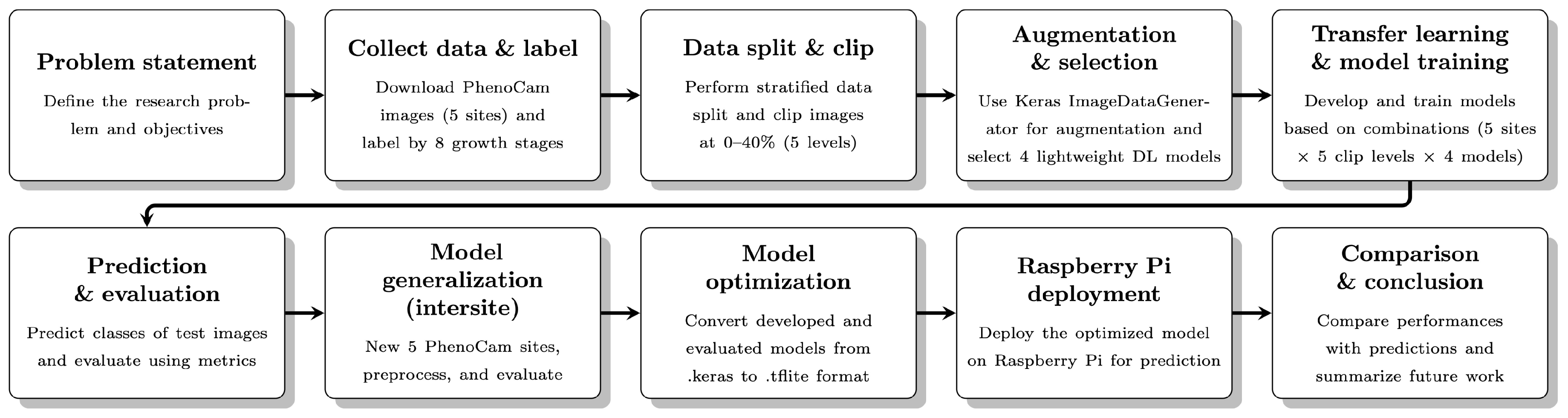
Figure 2.
Selected ten PhenoCam sites planted with corn across the USA for the year 2023–2025. IaS is intrasite, and IS is intersite.
Figure 2.
Selected ten PhenoCam sites planted with corn across the USA for the year 2023–2025. IaS is intrasite, and IS is intersite.
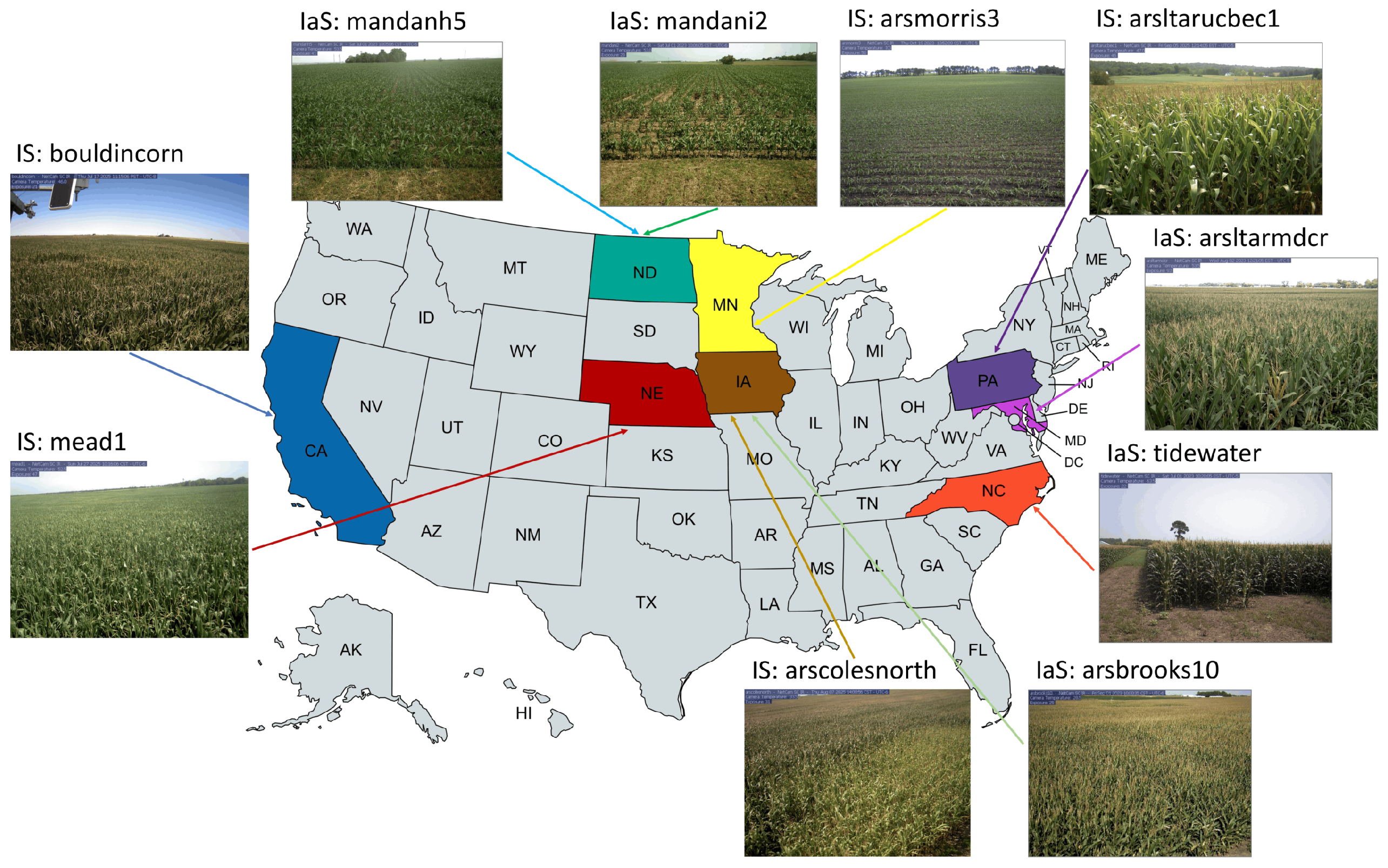
Figure 3.
Individual corn growth stages identified from PhenoCam images with manually assigned visual class labels.
Figure 3.
Individual corn growth stages identified from PhenoCam images with manually assigned visual class labels.
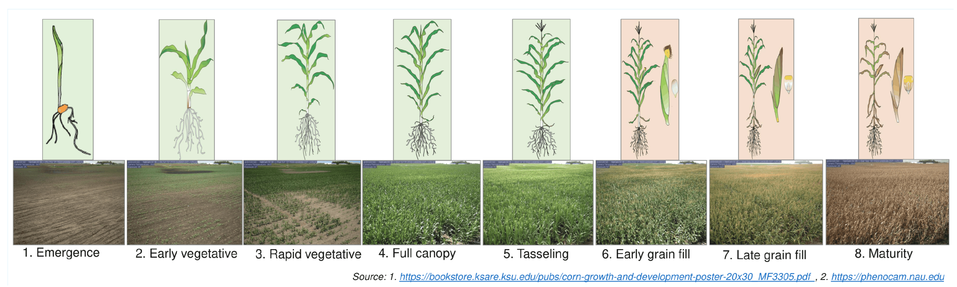
Figure 4.
Overall lightweight deep learning model development pipeline for PhenoCam image classification showing various stages in a supercomputer after transitioning from Google Colab.
Figure 4.
Overall lightweight deep learning model development pipeline for PhenoCam image classification showing various stages in a supercomputer after transitioning from Google Colab.
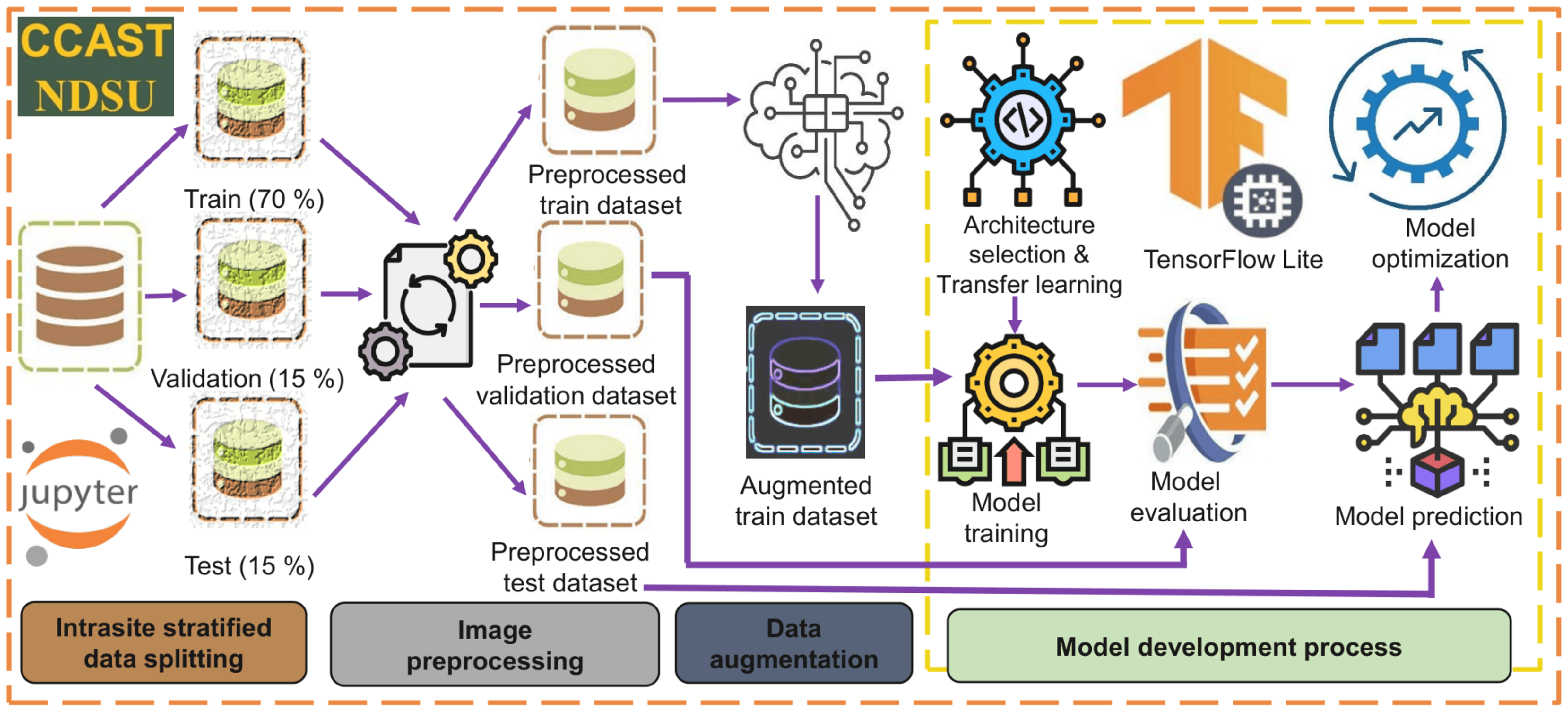
Figure 5.
An example of PhenoCam resized original image and an augmented image (rotated and padded) of size pixels that are used in model training. The augmentation method used rescaling, shear, zoom, horizontal flip, brightness, and shifting, while these outputs are not shown.
Figure 5.
An example of PhenoCam resized original image and an augmented image (rotated and padded) of size pixels that are used in model training. The augmentation method used rescaling, shear, zoom, horizontal flip, brightness, and shifting, while these outputs are not shown.
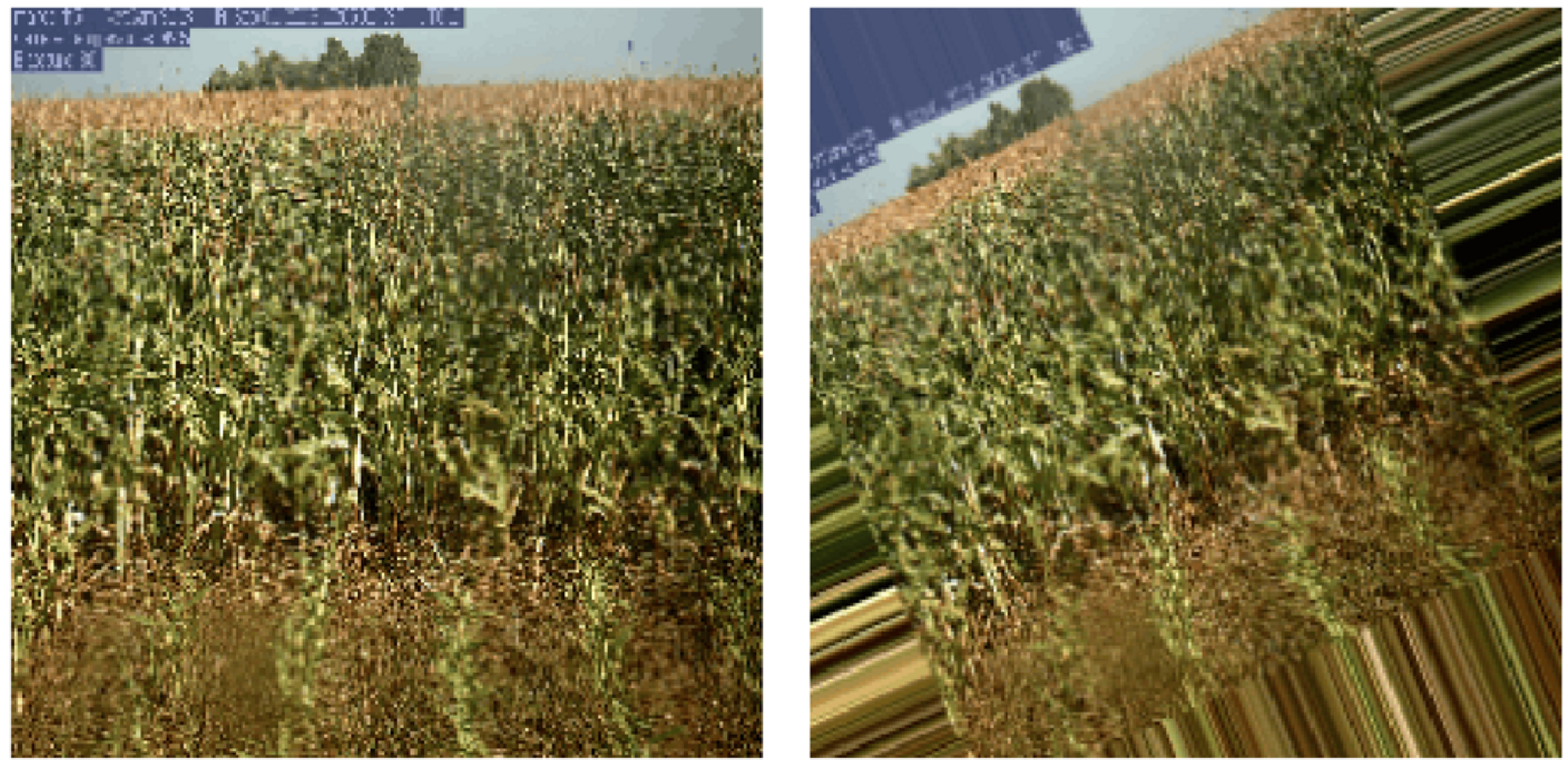
Figure 6.
Custom model design process through transfer learning for corn growth stage classification using the PhenoCam dataset.
Figure 6.
Custom model design process through transfer learning for corn growth stage classification using the PhenoCam dataset.
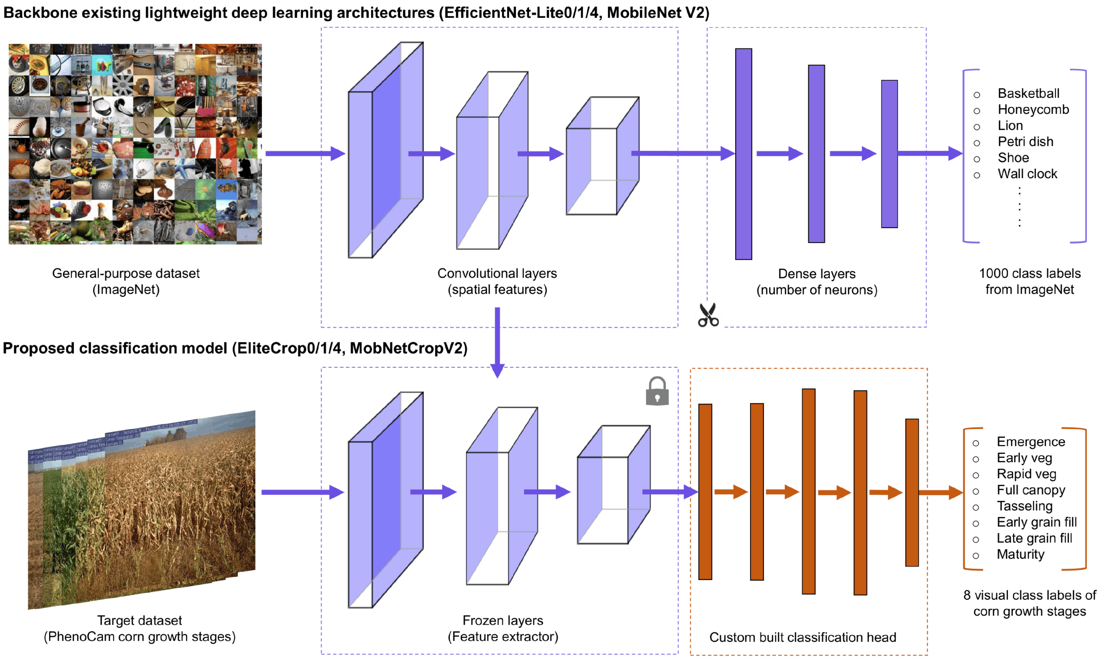
Figure 7.
Processes involved in deployment of lightweight deep learning models on Raspberry Pi and a sample corn stages classification results.
Figure 7.
Processes involved in deployment of lightweight deep learning models on Raspberry Pi and a sample corn stages classification results.
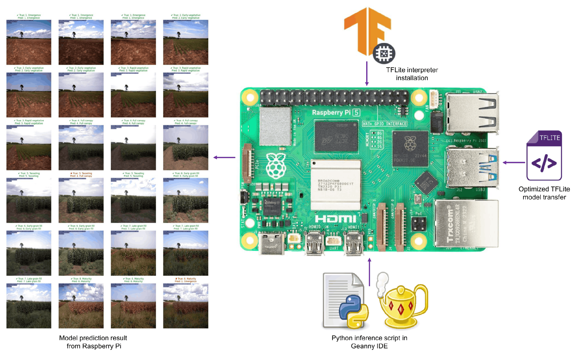
Figure 8.
Proportional distribution of corn growth stages across dataset splits for PhenoCam site arsbrooks10, taken for example. The outer ring (between dotted lines) represents the original data distribution, and concentric rings inwards represent train, validation, and test splits (pointed by the blue arrow), respectively.
Figure 8.
Proportional distribution of corn growth stages across dataset splits for PhenoCam site arsbrooks10, taken for example. The outer ring (between dotted lines) represents the original data distribution, and concentric rings inwards represent train, validation, and test splits (pointed by the blue arrow), respectively.
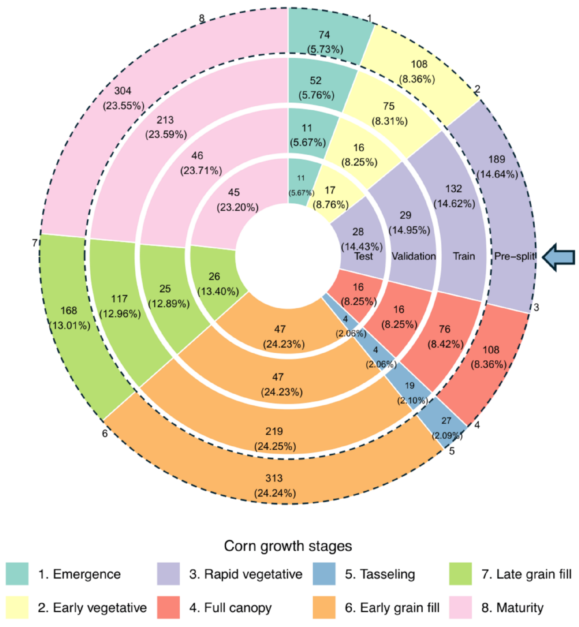
Figure 9.
Comparison of mean classification performance metrics for the developed lightweight deep learning models. Each bar represents the combined results of five PhenoCam sites and five image clipping levels (0%–40%) with mean difference significance labels ().
Figure 9.
Comparison of mean classification performance metrics for the developed lightweight deep learning models. Each bar represents the combined results of five PhenoCam sites and five image clipping levels (0%–40%) with mean difference significance labels ().
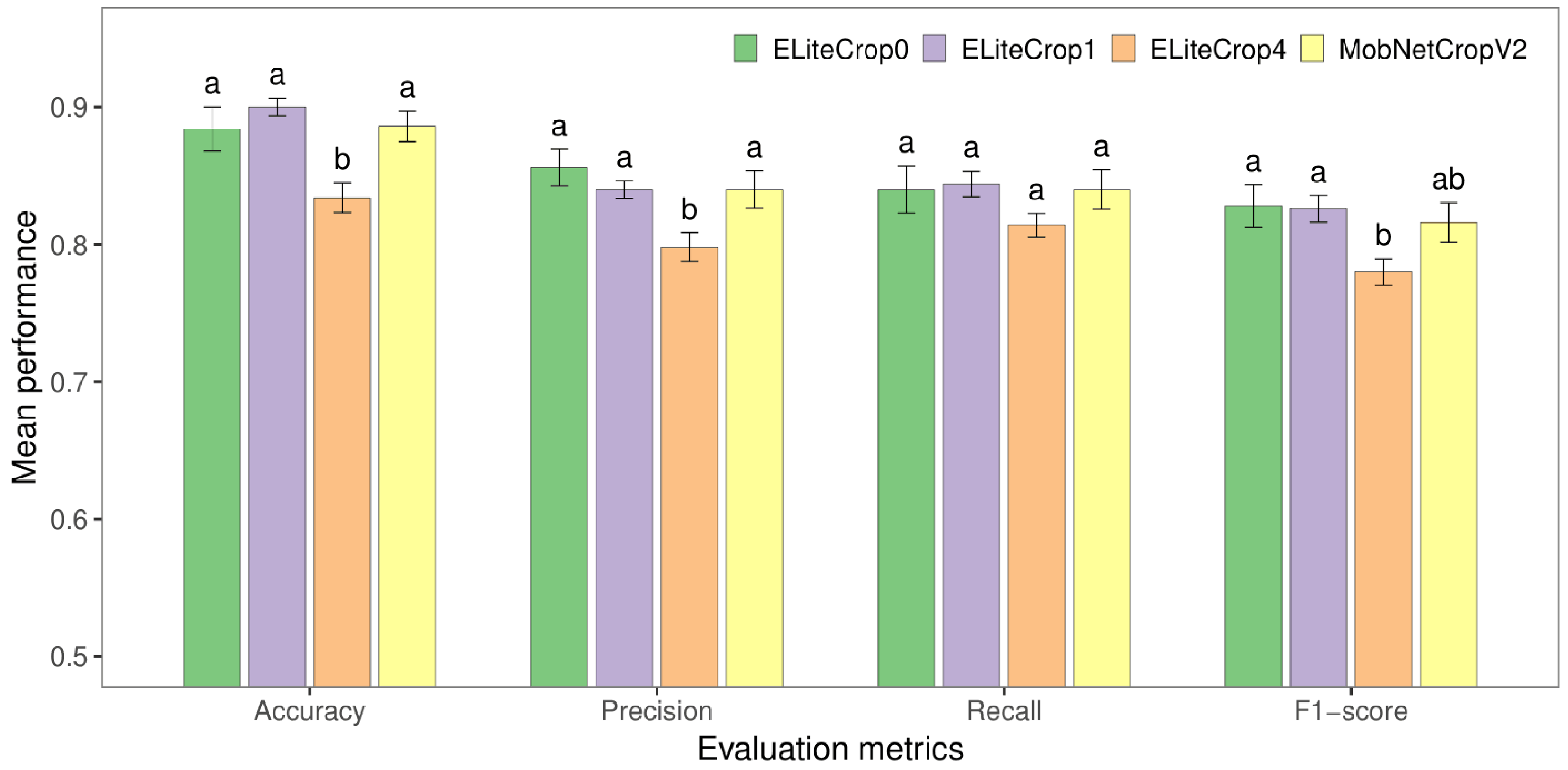
Figure 10.
Effect of PhenoCam image clipping levels on evaluation metrics of lightweight DL models and PhenoCam sites. (a) Performance evaluation of ELiteCrop0 for arsbrooks10 (PhenoCam site 1) across different image clipping levels. (b) Overall performance comparison of all models (4) and sites (5) under various image clipping levels.
Figure 10.
Effect of PhenoCam image clipping levels on evaluation metrics of lightweight DL models and PhenoCam sites. (a) Performance evaluation of ELiteCrop0 for arsbrooks10 (PhenoCam site 1) across different image clipping levels. (b) Overall performance comparison of all models (4) and sites (5) under various image clipping levels.
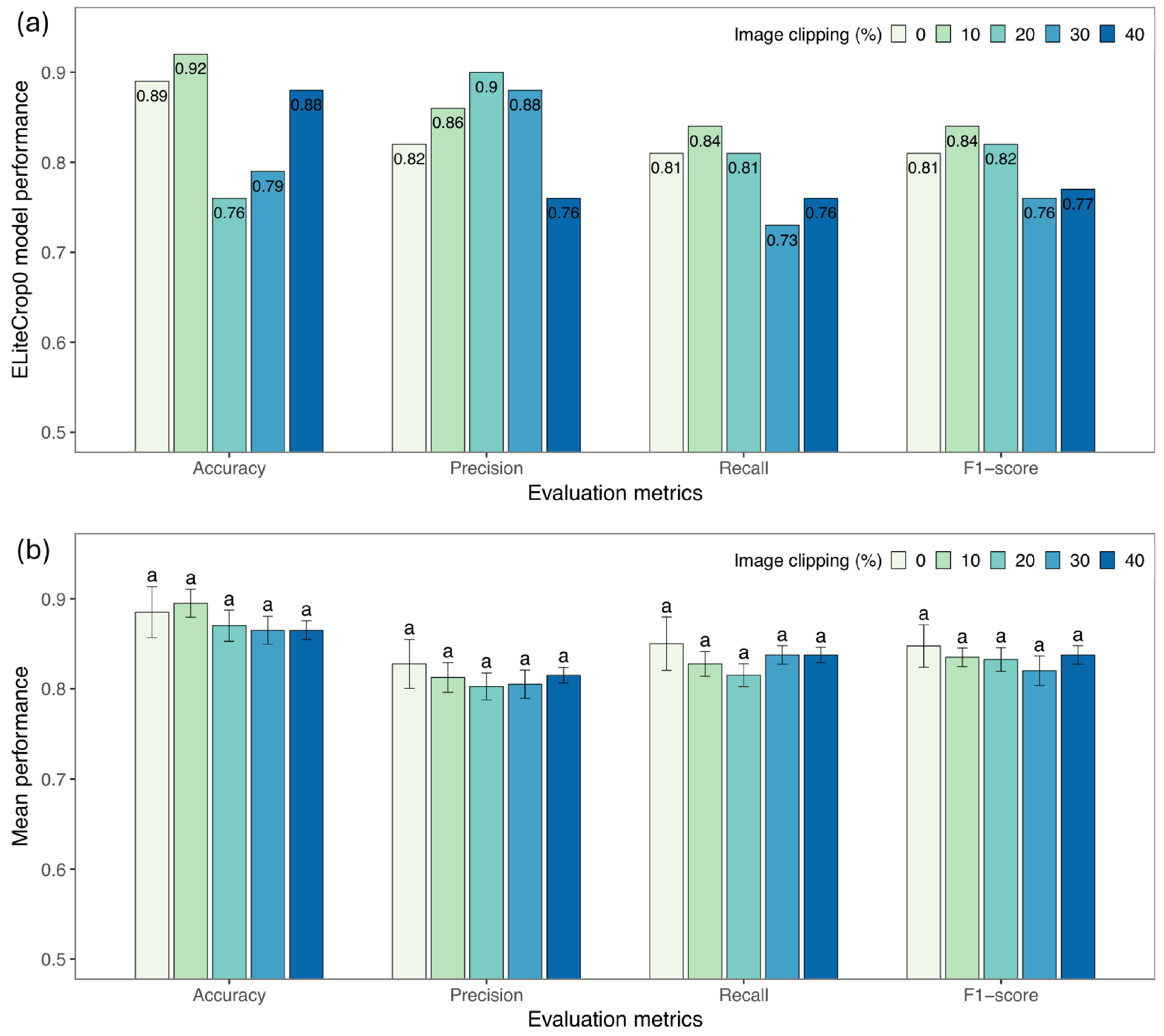
Figure 11.
Effect of PhenoCam image clipping levels (0–40%) on computational performance of lightweight DL models (ELiteCrop0, ELiteCrop1, ELiteCrop4, and MobNetCropV2). (a) Training time, (b) Testing time, and (c) Overall stacked time with numerical values.
Figure 11.
Effect of PhenoCam image clipping levels (0–40%) on computational performance of lightweight DL models (ELiteCrop0, ELiteCrop1, ELiteCrop4, and MobNetCropV2). (a) Training time, (b) Testing time, and (c) Overall stacked time with numerical values.
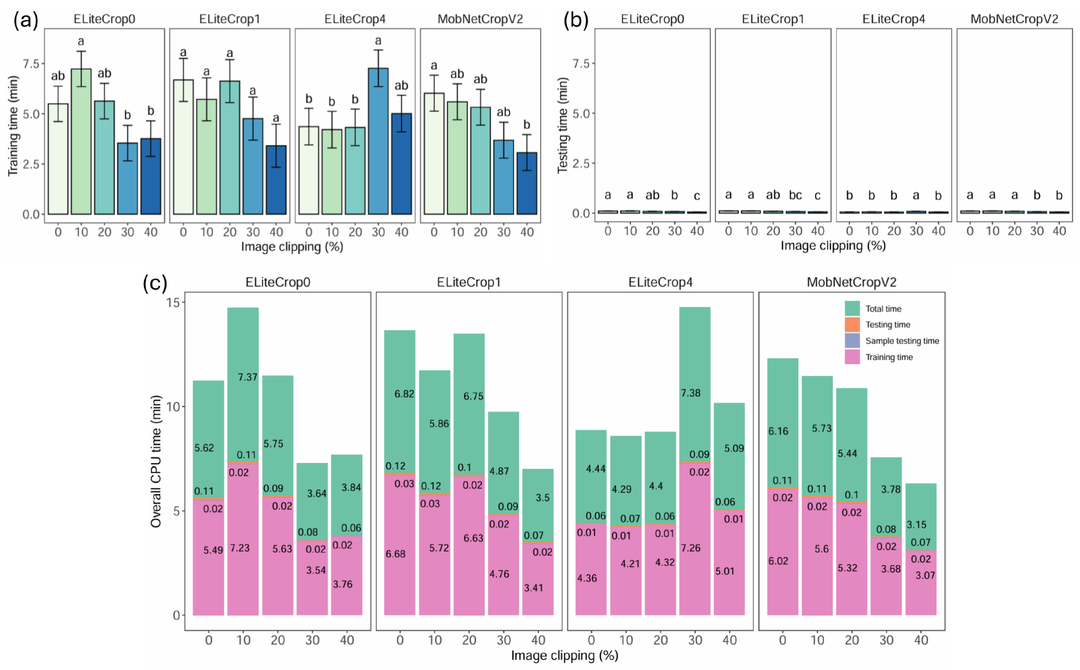
Figure 12.
Cumulative confusion matrix of the developed lightweight DL models’ predictions combining all sites and clipping levels on PhenoCam intrasite datasets using the developed novel “confusion matrix diagonal ratio” (CMDR).
Figure 12.
Cumulative confusion matrix of the developed lightweight DL models’ predictions combining all sites and clipping levels on PhenoCam intrasite datasets using the developed novel “confusion matrix diagonal ratio” (CMDR).
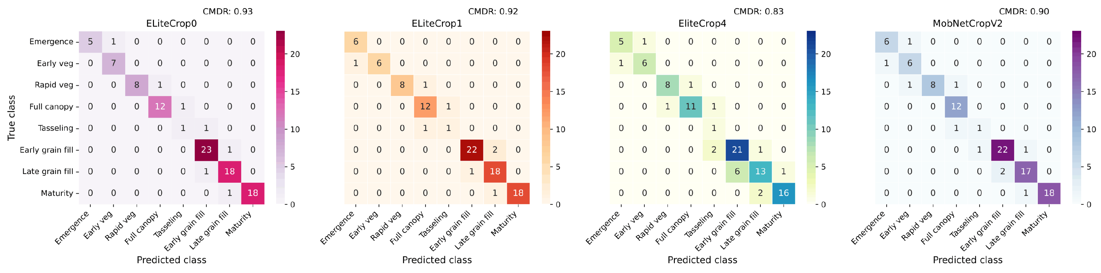
Figure 13.
Predicted corn growth stages of test images (randomized representative sample for each growth stage) using the finalized ELiteCrop0 model for arsltarmdcr Maryland PhenoCam site at 10% image clipping level.
Figure 13.
Predicted corn growth stages of test images (randomized representative sample for each growth stage) using the finalized ELiteCrop0 model for arsltarmdcr Maryland PhenoCam site at 10% image clipping level.
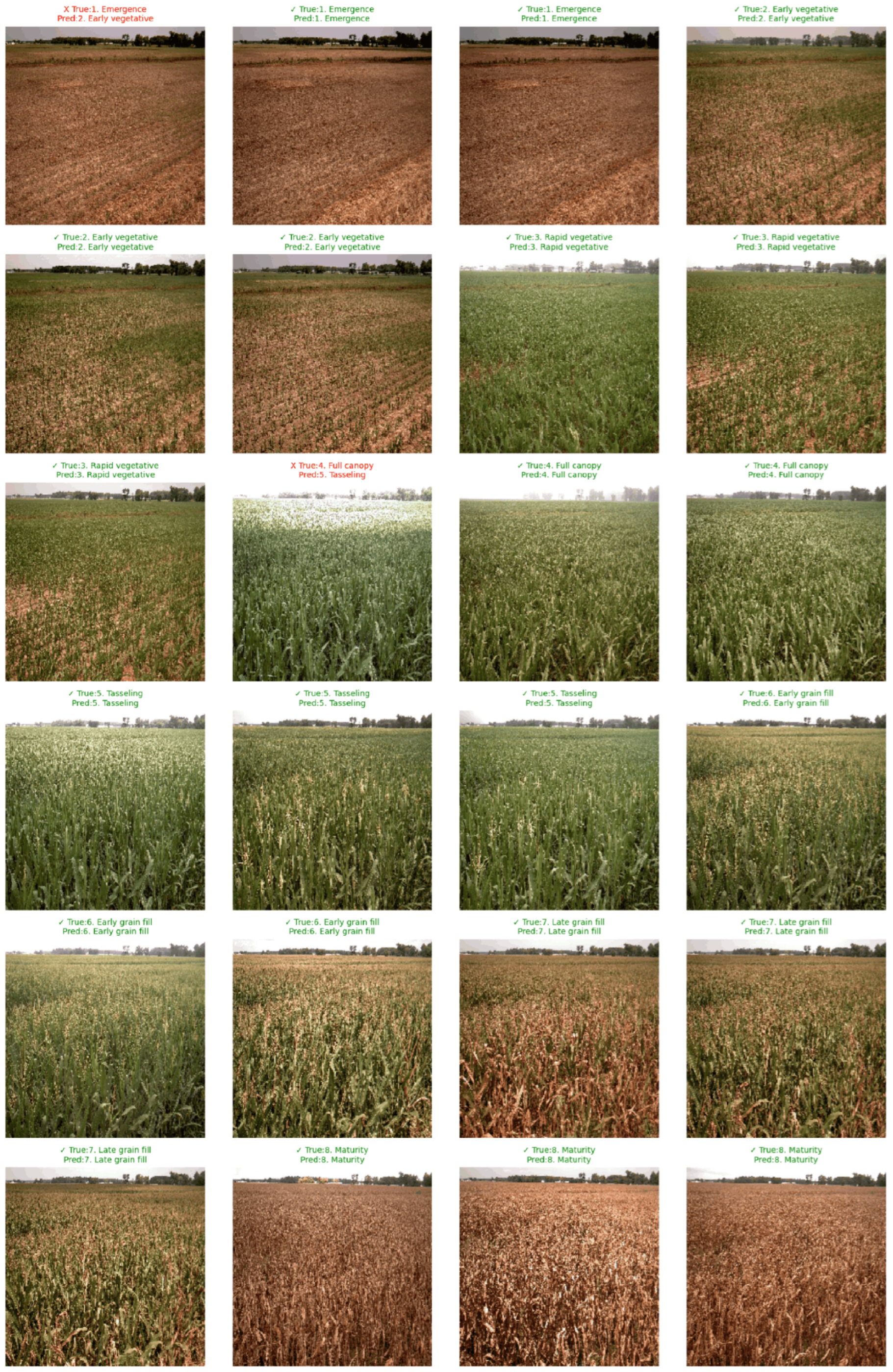
Figure 14.
Comparison of system configuration (CCAST and Raspberry Pi) for ELiteCrop0 model for intrasite (train + test on same train sites) and intersite (test on new sites) techniques.
Figure 14.
Comparison of system configuration (CCAST and Raspberry Pi) for ELiteCrop0 model for intrasite (train + test on same train sites) and intersite (test on new sites) techniques.
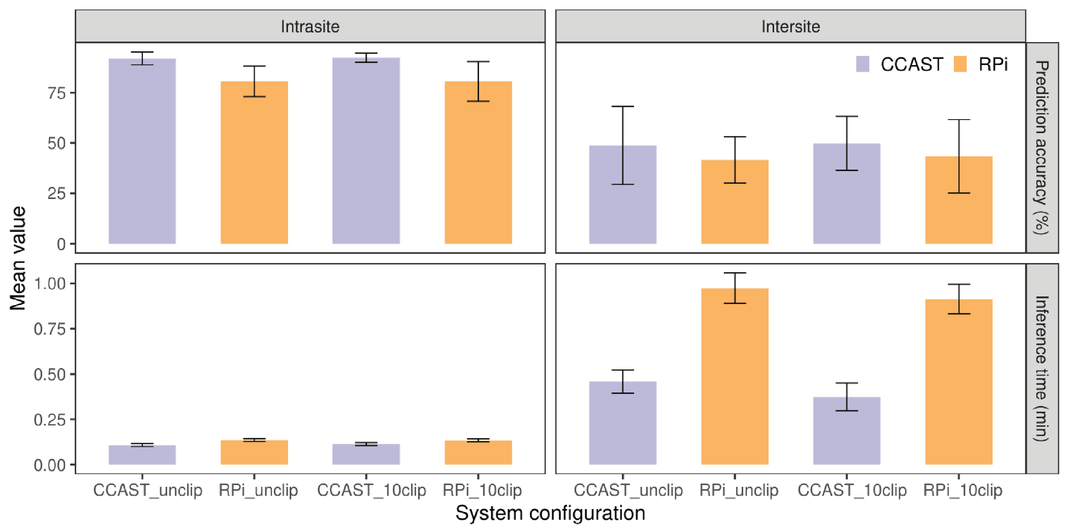

Table 1.
Geographical and environmental characteristics of chosen PhenoCam study sites.
| Category | PhenoCam site | Geographical coordinate | Elevation (m) | Climatic condition | Mean annual temperature (°C) | Mean annual precipitation (mm) | Soil type | Area (ha) |
|---|---|---|---|---|---|---|---|---|
| arsbrooks10 (Iowa) | 41.975°N, 93.691°W | 312 | Humid continental | 8.95 | 842 | Clarion loam | 35 | |
| arsltarmdcr (Maryland) | 39.058°N, 75.851°W | 17 | Humid continental | 13.3 | 1118 | Silt loam | 15 | |
| Intrasite | mandanh5 (North Dakota) | 46.775°N, 100.951°W | 593 | Semi-arid continental | 5.4 | 420 | Silt loam | 22.3 |
| mandani2 (North Dakota) | 46.761°N, 100.926°W | 590 | Semi-arid continental | 4 | 457 | Silt loam | 1.3 | |
| tidewater (North Carolina) | 35.850°N, 76.650°W | 5 | Humid subtropical | 16 | 1096 | Silt loam | 22.3 | |
| bouldincorn (California) | 38.109°N, 121.535°W | -5 | Mediterranean | 16 | 338 | Rindge muck | 15 | |
| arsltarucbec1 (Pennsylvania) | 40.753°N, 78.005°W | 400 | Humid continental | 10 | 1168 | Silt loam | 14 | |
| Intersite | mead1 (Nebraska) | 41.165°N, 96.476°W | 361 | Humid continental | 10 | 790 | Silty clay loam | 49 |
| arsmorris3 (Minnesota) | 45.609°N, 96.126°W | 342 | Continental | 7 | 673 | Clay loam | 3 | |
| arscolesnorth (Iowa) | 42.488°N, 93.522°W | 356 | Humid continental | 10 | 906 | Clay loam | 32 |
Table 2.
Classified corn growth stages from PhenoCam images based on visual class labels.
| Visual class labels | Visual appearance |
|---|---|
| 1. Emergence | Soil mostly visible, few green shoots |
| 2. Early vegetative | Rows visible, small leaves |
| 3. Rapid vegetative | Fast canopy expansion, closing rows |
| 4. Full canopy | Dense uniform green |
| 5. Tasseling | Tassels visible, lighter top hue |
| 6. Early grain fill | Yellowing, patchy canopy |
| 7. Late grain fill | Brown, senescing tassels |
| 8. Maturity | Browning of leaves and plant |
Table 3.
Cumulative comparison of accuracy and loss metrics across four lightweight deep learning models and five PhenoCam sites.
Table 3.
Cumulative comparison of accuracy and loss metrics across four lightweight deep learning models and five PhenoCam sites.
| Model | PhenoCam site | Training accuracy | Validation accuracy | Training loss | Validation loss | ||||||||
|---|---|---|---|---|---|---|---|---|---|---|---|---|---|
| Min | Max | Avg ± Std | Min | Max | Avg ± Std | Min | Max | Avg ± Std | Min | Max | Avg ± Std | ||
| EliteCrop0 | s1 | 0.477 | 0.813 | 0.732 ± 0.096 | 0.624 | 0.842 | 0.467 | 1.439 | 0.479 | 0.986 | |||
| s2 | 0.481 | 0.881 | 0.616 | 0.849 | 0.333 | 1.450 | 0.407 | 1.092 | |||||
| s3 | 0.486 | 0.861 | 0.658 | 0.933 | 0.395 | 1.632 | 0.293 | 0.834 | |||||
| s4 | 0.485 | 0.856 | 0.688 | 0.867 | 0.394 | 1.427 | 0.366 | 0.808 | |||||
| s5 | 0.392 | 0.890 | 0.701 | 0.942 | 0.266 | 1.645 | 0.182 | 0.953 | |||||
| Avg | 0.464 | 0.860 | 0.657 | 0.887 | 0.371 | 1.519 | 0.345 | 0.935 | |||||
| EliteCrop1 | s1 | 0.479 | 0.777 | 0.653 | 0.839 | 0.550 | 1.438 | 0.514 | 0.953 | ||||
| s2 | 0.478 | 0.880 | 0.657 | 0.893 | 0.329 | 1.475 | 0.321 | 1.003 | |||||
| s3 | 0.458 | 0.851 | 0.658 | 0.931 | 0.424 | 1.781 | 0.309 | 0.923 | |||||
| s4 | 0.483 | 0.837 | 0.672 | 0.891 | 0.418 | 1.404 | 0.383 | 0.895 | |||||
| s5 | 0.413 | 0.877 | 0.648 | 0.933 | 0.293 | 1.607 | 0.222 | 1.000 | |||||
| Avg | 0.462 | 0.845 | 0.657 | 0.897 | 0.403 | 1.541 | 0.350 | 0.955 | |||||
| EliteCrop4 | s1 | 0.427 | 0.797 | 0.519 | 0.796 | 0.486 | 1.535 | 0.544 | 1.205 | ||||
| s2 | 0.509 | 0.840 | 0.561 | 0.787 | 0.451 | 1.334 | 0.516 | 1.082 | |||||
| s3 | 0.450 | 0.831 | 0.553 | 0.864 | 0.460 | 1.604 | 0.422 | 1.092 | |||||
| s4 | 0.438 | 0.866 | 0.508 | 0.873 | 0.365 | 1.496 | 0.365 | 1.035 | |||||
| s5 | 0.373 | 0.858 | 0.450 | 0.832 | 0.355 | 1.632 | 0.469 | 1.245 | |||||
| Avg | 0.439 | 0.838 | 0.518 | 0.830 | 0.423 | 1.520 | 0.463 | 1.132 | |||||
| MobNetCropV2 | s1 | 0.452 | 0.787 | 0.639 | 0.828 | 0.502 | 1.552 | 0.448 | 0.899 | ||||
| s2 | 0.481 | 0.880 | 0.728 | 0.899 | 0.314 | 1.491 | 0.297 | 0.679 | |||||
| s3 | 0.483 | 0.840 | 0.637 | 0.895 | 0.409 | 1.790 | 0.297 | 0.928 | |||||
| s4 | 0.477 | 0.821 | 0.632 | 0.868 | 0.455 | 1.556 | 0.360 | 0.811 | |||||
| s5 | 0.405 | 0.873 | 0.710 | 0.911 | 0.333 | 1.554 | 0.254 | 0.669 | |||||
| Avg | 0.460 | 0.840 | 0.669 | 0.880 | 0.403 | 1.589 | 0.331 | 0.797 | |||||
PhenoCam sites name: s1 - arsbrooks10, s2 - arsltarmdcr, s3 - mandanh5, s4 - mandani2, s5 - tidewater. Accuracy values are in decimals. The range of loss values is from to . The individual PhenoCam site values are the cumulative values across five different image clipping levels.
Disclaimer/Publisher’s Note: The statements, opinions and data contained in all publications are solely those of the individual author(s) and contributor(s) and not of MDPI and/or the editor(s). MDPI and/or the editor(s) disclaim responsibility for any injury to people or property resulting from any ideas, methods, instructions or products referred to in the content. |
© 2026 by the authors. Licensee MDPI, Basel, Switzerland. This article is an open access article distributed under the terms and conditions of the Creative Commons Attribution (CC BY) license (http://creativecommons.org/licenses/by/4.0/).
Copyright: This open access article is published under a Creative Commons CC BY 4.0 license, which permit the free download, distribution, and reuse, provided that the author and preprint are cited in any reuse.