

Submitted:
06 August 2026
Posted:
10 August 2026
You are already at the latest version
Abstract
The Traveling Salesman Problem (TSP) is a representative NP-hard combinatorial optimization problem whose search space grows rapidly with the number of cities. Classical ant colony optimization (ACO) is attractive because of its distributed construction process and positive-feedback search, but its performance deteriorates on large instances owing to probability dilution, pheromone concentration, search stagnation, and the cost of optimizing a complete tour with a single colony. This paper proposes Collaborative Attention Ant Colony Optimization (CAACO), which integrates sparse coordinate-based graph attention, random-offset collaborative subpath optimization, a memetic MAX–MIN Ant System, and adaptive double-bridge stagnation escape. The method is evaluated against FACO, BCACO, and CCACO on nine symmetric Euclidean TSP instances, with every algorithm executed independently 30 times per instance. CAACO obtains the lowest mean GAP on all nine instances, with an average instance-level mean GAP of 3.193%, compared with 12.587%, 22.177%, and 23.826% for the three baselines. Per-instance two-sided Mann–Whitney U tests with Holm correction show significant differences in all 27 comparisons (pHolm < 10−10), and the Vargha–Delaney effect size is A12=1.000 throughout. These results demonstrate a consistently favorable solution-quality distribution for the proposed framework, while the runtime analysis shows a quality–efficiency trade-off relative to the efficiency-oriented baseline. A 30-run ablation study further shows that removing attention, dynamic slicing, and double-bridge escape increases the average mean GAP from 3.199% to 4.525%, 5.863%, and 3.813%, respectively; all 27 module-level comparisons remain significant after Holm correction.
Keywords:
ant colony optimization
; attention mechanism
; collaborative optimization
; MAX–MIN Ant System
; traveling salesman problem
; large-scale combinatorial optimization
1. Introduction
The Traveling Salesman Problem (TSP) asks for a minimum-length Hamiltonian cycle through a set of cities. Despite its concise definition, the TSP is one of the most influential NP-hard problems in combinatorial optimization and has served as a benchmark for exact algorithms, approximation methods, local search, and metaheuristics [1,2,4]. Practical variants arise in vehicle routing, printed-circuit-board drilling, tool-path planning, chip manufacturing, inspection, sequencing, and network design. As the number of cities grows into the thousands or tens of thousands, exhaustive enumeration and many exact techniques become computationally prohibitive, making high-quality heuristic search essential.
Ant colony optimization (ACO) models the indirect communication of natural ants through pheromone trails. Artificial ants construct tours probabilistically according to pheromone intensity and heuristic information, after which favorable edges receive reinforcement [5,8]. ACO has a number of attractive properties for TSP search: its solution construction process is naturally distributed, its probabilistic rule supports exploration, and its pheromone memory promotes exploitation. The Ant Colony System (ACS) and MAX–MIN Ant System (MMAS) improve the original Ant System through local pheromone updates, elitist reinforcement, and explicit pheromone bounds [6,7].
Nevertheless, four difficulties become pronounced on large TSP instances. First, evaluating all unvisited cities at every construction step creates a large denominator in the transition rule and weakens the contrast between promising and unpromising candidates. Second, repeated reinforcement can concentrate pheromone on a limited set of edges, causing premature convergence. Third, optimizing a complete tour with one colony couples all decisions and produces a very large effective search space. Fourth, a single perturbation intensity is insufficient because shallow stagnation and deep local trapping require different search responses.
Two lines of research provide useful ingredients for addressing these limitations. Candidate-set and local-search methods restrict expensive evaluations to promising neighborhoods and refine tours using edge exchanges such as 2-opt, 3-opt, and Lin–Kernighan moves [9,10,11,12]. Attention mechanisms provide a data-dependent way to score relationships between nodes and have been successfully applied to graph representation and learned routing policies [15,16,17,18]. However, fully learned routing models often require substantial training data and may not transfer transparently to new instance distributions. A lightweight attention prior embedded in an interpretable metaheuristic can preserve the search flexibility of ACO while improving candidate discrimination.
Collaborative optimization offers a complementary perspective. A large solution can be decomposed into interacting components that are optimized separately and periodically coordinated [27]. For a TSP tour, contiguous subpaths form natural components, but fixed segmentation introduces boundary artifacts: edges near permanent boundaries receive less opportunity for improvement. A dynamic random-offset partition can remove this bias, and concurrent optimization can exploit multicore processors without abandoning global tour consistency.
Motivated by these observations, this work proposes Collaborative Attention Ant Colony Optimization (CAACO). The method uses sparse graph self-attention to generate a city-neighborhood prior, dynamically slices the current tour into contiguous subpaths, optimizes these subpaths in parallel using a memetic MMAS, and applies adaptive double-bridge perturbation when global progress stalls. Unlike end-to-end neural construction, the attention component is used only as an interpretable search prior; tour quality remains determined by explicit probabilistic construction, pheromone learning, local search, and global acceptance.
The principal contributions are as follows:
- A sparse graph self-attention preprocessing mechanism is introduced to combine coordinate-derived structural similarity, distance bias, and neighborhood restriction in the ACO transition rule.
- A random-offset dynamic slicing framework is developed to optimize multiple contiguous subpaths concurrently while varying slice boundaries across global iterations.
- A memetic MMAS subsolver combines pheromone bounds, attention-guided state transitions, elite reinforcement, and iteration-best 2-opt refinement.
- A two-level stagnation escape strategy integrates non-inferiority roaming with mild and severe double-bridge perturbations, improving the ability to leave local optima without discarding the global incumbent.
- Thirty independent runs per algorithm and instance show that CAACO has the lowest mean GAP on all nine benchmarks. All 27 per-instance rank-sum comparisons remain significant after Holm correction (), with .
- A controlled 30-run ablation study verifies the independent contribution of all three modules. Removing attention, dynamic slicing, and double-bridge escape increases the average mean GAP by 1.326, 2.664, and 0.614 percentage points, respectively.
The remainder of this paper is organized as follows. Section 2 reviews ACO, local search, attention-based routing, and collaborative large-scale optimization. Section 3 presents the TSP formulation and the complete CAACO method. Section 4 describes the benchmarks, implementation settings, comparison algorithms, repeated-run outcomes, ablation results, and statistical evaluation procedure. Section 5 discusses the mechanisms, trade-offs, limitations, and threats to validity. Section 6 concludes the paper.
2. Related Work
2.1. Recent Ant Colony Optimization for Large-Scale TSP
Ant System, Ant Colony System (ACS), and MAX–MIN Ant System (MMAS) established the core constructive, local-update, and bounded-pheromone mechanisms used by modern ACO solvers [5,6,7]. These foundational studies remain necessary references, but recent TSP work has increasingly emphasized scale, adaptive control, and hybrid local improvement. Heterogeneous adaptive ACO with 3-opt combines colony diversity with intensive tour refinement [35], while dynamic evaporation, parameter optimization, and visibility adaptation alter the balance between exploration and exploitation during construction [36,38,41]. Memory-efficient data structures, adaptive node clustering, and dynamic-demand studies have clarified how representation and changing edge costs affect ACO at scale [37,39,40]. Other recent methods use adaptive greedy rules, dynamic hybrid mechanisms, or scale-aware parameter adaptation to improve robustness [42,43,46].
For large TSP instances, computational efficiency is inseparable from candidate management and local search. FACO was designed specifically to improve ACO efficiency on large instances [30]. Heuristic-smoothing ACO introduces differential information to stabilize and accelerate search [44], whereas finite-history archiving and game-based mechanisms preserve useful colony information without indefinitely accumulating pheromone [45]. A heterogeneous selective-evolution design further demonstrates the continuing shift from a single homogeneous colony toward role-specialized populations [47]. Collectively, these studies indicate that large-scale performance depends on restricting expensive decisions, retaining diverse historical information, and coupling construction with strong local improvement rather than merely increasing the number of ants or iterations.
2.2. Collaborative and Multi-Colony ACO
Collaborative ACO distributes search responsibility among colonies and defines mechanisms for information exchange. The cooperative-game CCACO method allocates multi-colony contributions through a game-theoretic mechanism [29]. Dynamic collaborative ACO combines heterogeneous ACS and MMAS populations, pheromone fusion, and path recommendation [32]. BCACO adds bidirectional induction and cooperative-game interaction to balance convergence and diversity on large TSP instances [31]. Related game-based and pheromone-refactoring methods use strategic payoff allocation or correlation-guided information exchange to prevent one colony from dominating the search [33,34].
These multi-colony studies improve information sharing, but they generally coordinate complete-tour populations. Cooperative coevolution suggests an alternative: decompose a high-dimensional solution into interacting components that can be optimized separately [27,28]. For TSP, naive fixed decomposition can create persistent boundary edges, and fully independent subproblems can damage global consistency. The proposed method therefore decomposes the current tour into contiguous endpoint-constrained slices, changes the offset between global iterations, optimizes slices concurrently, and performs whole-tour stitching after reassembly. This differs from multi-colony complete-tour competition because collaboration occurs at the subpath, reassembly, and iteration levels.
2.3. Attention and Learning-Guided Routing
Scaled dot-product attention and graph attention provide general mechanisms for assigning content-dependent importance to nodes and edges [15,16]. Attention models subsequently became a major paradigm for learned routing [18], with POMO exploiting multiple solution symmetries and efficient active search adapting a pretrained model at test time [19,20]. Surveys of reinforcement learning and machine learning for combinatorial optimization summarize the rapid development of these approaches and their generalization challenges [21,22,23].
Recent neural-metaheuristic hybrids are especially relevant to ACO. Learning-based Neural ACO predicts heuristic information while retaining ant-based sampling [24], and DeepACO uses neural guidance to strengthen ant-system construction across combinatorial problems [25]. Diffusion-based solvers such as DIFUSCO learn distributions over promising graph structures rather than directly reproducing a classical local-search trajectory [26]. These methods can achieve strong performance, but they require training data, model selection, and distributional assumptions. In contrast, CAACO uses no learned parameters: its attention score is a deterministic structural prior computed from the current coordinates and sparse neighborhoods, while pheromone, 2-opt, and double-bridge moves remain explicit and auditable.
2.4. Tour Improvement, Perturbation, and Research Gap
The 2-opt, 3-opt, and Lin–Kernighan families remain central to high-performance TSP search because they convert a constructed tour into a local optimum under progressively richer edge-exchange neighborhoods [9,10,11,12]. Iterated local search uses stronger perturbations to move between attraction basins; the double-bridge move is a standard non-sequential perturbation that cannot be reduced to one 2-opt exchange [13,14]. Recent ACO variants confirm that selective application of local search can provide substantial quality gains without applying an expensive improvement pass to every ant [30,35].
The literature therefore provides four mature but usually separate ingredients: bounded pheromone learning, collaborative multi-colony exchange, attention or neural edge guidance, and perturbation-based local search. Fewer studies integrate these elements within a training-free, dynamically decomposed framework for tens-of-thousands-city TSP instances. CAACO addresses this gap by combining a transparent sparse attention prior, random-offset subpath decomposition, parallel memetic MMAS, whole-tour stitching, non-inferiority roaming, and two-level double-bridge escape in one implementation.
3. Materials and Methods
3.1. Problem Formulation
A symmetric Euclidean TSP instance is represented by a complete graph , where is the city set and E is the edge set. City i has coordinate . The rounded Euclidean distance is denoted by . A feasible tour is a permutation followed by a return to . Its length is
The objective is to find .
3.2. Overview of the CAACO Framework
Figure 1 summarizes the method. City coordinates are normalized and converted into a sparse attention matrix. An initial global tour is then produced from the attention-guided neighborhood information. At every global iteration, the tour is cut into contiguous slices using a randomly shifted boundary. Each slice is optimized independently and concurrently by a memetic MMAS while its endpoints remain fixed. The improved slices are reassembled, a global 2-opt stitching pass is applied, and the incumbent and stagnation counters are updated. If the search has not improved for a specified number of global iterations, a mild or severe double-bridge perturbation is triggered and the process returns to dynamic slicing.
3.3. Sparse Graph Self-Attention Preprocessing
Let the coordinate centroid be
The centered coordinate of city i is . A two-dimensional query/key feature is defined as
where avoids division by zero.
For each city, attention is evaluated only on a K-nearest-neighbor set . The compatibility score combines directional similarity and a distance bias:
where and scales the distance prior. Numerically stable softmax normalization gives
The matrix is sparse because outside . Attention is not treated as a learned optimal policy; it is a deterministic structural prior derived from the current instance. The attention-guided heuristic is
where controls attention influence and small constants keep every admissible candidate reachable.
With a precomputed or spatially indexed KNN graph, the number of attention entries is instead of . If a brute-force KNN construction is used, preprocessing still requires distance evaluations; this distinction is important when interpreting scalability.
3.4. Dynamic Random-Offset Slicing
Let the current cyclic tour be . At global iteration t, a slice length is sampled from
A random offset rotates the starting position before partitioning. This produces contiguous subpaths. Because changes across iterations, an edge that lies on a boundary in one iteration can be placed inside a slice in a later iteration.
Each slice contains fixed left and right hinge cities inherited from the global tour. Internal cities may be reordered, but the hinges remain fixed so that independently optimized slices can be reassembled without violating feasibility. Slices are submitted to independent worker threads. Collaboration occurs through three channels:
- 1.
- path collaboration: every subsolver receives the current global slice and returns an improved feasible subpath;
- 2.
- pheromone collaboration: the global incumbent influences the initialization and bounds of local pheromone matrices;
- 3.
- iteration collaboration: reassembled tours are globally stitched and become the parent tours for subsequent random-offset partitions.
3.5. Attention-Guided Memetic MMAS Subsolver
Within a slice, ant k at city i selects an admissible city j according to
where is the set of unvisited admissible cities, controls pheromone influence, and controls heuristic influence. The fixed terminal hinge is withheld from ordinary selection and inserted at the end of the subpath construction.
After all ants construct a subpath, only the iteration-best ant receives a full 2-opt pass. This memetic design concentrates local-search cost on the most promising solution while still allowing the colony to explore diverse constructions. Pheromone evaporation and reinforcement are
where is the evaporation rate and Q is a scale constant. MMAS bounds are set using the elite subpath length:
and every updated value is clipped to .
3.6. Global Reassembly and Non-Inferiority Roaming
The optimized slices are concatenated in their original cyclic order. A whole-tour 2-opt stitching pass then repairs suboptimal cross-boundary connections. Let be the stitched tour, , and be the best tour found so far. If , the incumbent is replaced and the stagnation counter is cleared. Otherwise, CAACO does not always revert the parent tour to . The feasible non-improving tour may remain the parent of the next slicing iteration. This non-inferiority roaming allows the search to traverse equal or moderately inferior regions while preserving separately as a safe incumbent.
3.7. Adaptive Double-Bridge Stagnation Escape
The stagnation counter s records consecutive global iterations without an incumbent improvement. Two perturbation levels are used:
- Mild escape: when , one double-bridge move is applied to , followed by 2-opt repair.
- Severe escape: when , where , two consecutive double-bridge moves are applied before 2-opt repair.
The experimental implementation uses and global non-improving iterations.
Figure 2 illustrates the operator. Four edges are removed, creating four segments A, B, C, and D. The segments are reconnected in a new non-sequential order, such as A–C–B–D, producing a move that cannot be reduced to one simple 2-opt exchange.
3.8. Complete Algorithm
Algorithm 1 gives the full procedure.
| Algorithm 1 Collaborative Attention Ant Colony Optimization (CAACO) |
|
3.9. Complexity Analysis
Assume a sparse neighborhood size K, m ants, a typical slice size h, slices, local MMAS iterations, and T global iterations. Sparse attention storage is . If KNN search is provided by a spatial index, attention construction is typically near ; brute-force KNN construction remains .
A direct ant construction within one slice costs if every unvisited internal city is considered, or approximately when a fixed candidate set is used with a fallback rule. Across all slices, sequential work per local iteration is approximately under candidate restriction. With p effective worker threads and balanced slices, the idealized wall-clock contribution is , although synchronization, unequal slice sizes, memory bandwidth, and 2-opt costs reduce practical speedup. A naive whole-tour 2-opt pass costs , while candidate-restricted or don’t-look-bit implementations can be substantially cheaper in practice. Thus, the practical complexity is governed by candidate construction, the local MMAS iteration budget, and the implementation of global 2-opt.
4. Experimental Results
4.1. Benchmark Instances and Evaluation Metrics
Nine symmetric Euclidean TSP instances were used. Eight are TSPLIB instances and one, bbz25234, is from the VLSI TSP collection [3,52]. Their sizes range from 280 to 25,234 cities. The best-known or optimal tour lengths used for GAP calculation are listed in Table 1. For d15112, the verified optimal value 1,573,084 is used consistently [53].
The principal quality metric is the percentage deviation from the BKS:
where is the tour length returned by an algorithm and is the best-known or optimal tour length for the corresponding instance. Lower GAP values indicate better solution quality. Runtime is reported in seconds.
Each of the four algorithms was executed independently 30 times on every instance, producing 1080 observations in total. Each observation contains the instance name, algorithm, run index, tour length, wall-clock runtime, and GAP. The input archive was audited before analysis: all 36 algorithm–instance groups contain exactly 30 observations with unique run indices from 1 to 30. The tables report sample means and sample standard deviations, and the inferential procedure is given in Section 4.7.
4.2. Parameter and Implementation Settings
Table 2 lists constants directly determined from the implementation and experiment records. The attention neighborhood contains at most 50 cities, the coordinate query/key dimension is two, the distance-bias coefficient is 100, and the numerical offsets used for coordinate normalization and inverse distance are . Euclidean distances are rounded according to the TSPLIB EUC_2D convention.
The local MMAS iteration count , slice-length interval , pheromone exponent , heuristic exponent , and evaporation rate are configuration-level parameters. Their notation is retained throughout the method description so that implementations can reproduce the same transition and pheromone-update equations.
4.3. Comparison Algorithms
Three published ACO methods are used as baselines. FACO denotes the efficiency-oriented ACO method for large TSP instances proposed by Skinderowicz [30]. BCACO denotes the bidirectional-induction and cooperative-game multi-ant-colony method of Wu et al. [31]. CCACO denotes the cooperative-game multi-colony collaborative ant optimization method of Meng et al. [29]. All comparison results are evaluated with the same BKS values listed in Table 1.
4.4. Thirty-Run Results of the Proposed Method
Table 3 summarizes the 30 independent CAACO runs on each instance. Across the nine instance-level mean values, the average GAP is 3.193%. The lowest mean GAP is obtained on a280 (0.033%), while the highest is obtained on pla7397 (5.179%). The standard deviation of GAP remains below 0.250 percentage points on every instance, indicating limited within-instance dispersion in the supplied 30-run observations.
4.5. Solution-Quality and Runtime Comparison
Table 4 reports the mean and sample standard deviation of GAP over 30 independent runs. CAACO obtains the lowest mean GAP on all nine instances. Averaged over the nine instance-level means, CAACO achieves 3.193%, compared with 12.587%, 22.177%, and 23.826% for FACO, BCACO, and CCACO, respectively. These values correspond to relative reductions of 74.6%, 85.6%, and 86.6%. The CAACO entries are typeset in bold because, for every instance, the 30-run mean is lower than all three baseline means and all three Holm-adjusted pairwise tests are significant at .
Table 5 gives the corresponding runtime distributions. CAACO is faster than both collaborative baselines on every instance in the supplied archive. FACO remains faster on several of the larger instances, but this speed advantage is accompanied by substantially higher mean GAP values.
4.6. Ablation Study
A controlled leave-one-module-out experiment was conducted to quantify the contribution of graph attention, dynamic slicing, and adaptive double-bridge escape. Four configurations were evaluated. Full CAACO retains the complete framework. CAACO-w/o-Att disables the sparse attention module, uses a nearest-neighbor initial tour, and sets the attention multiplier in the MMAS transition rule to . CAACO-w/o-Slice disables the random-offset dynamic slicing policy and uses fixed contiguous partitions with fixed boundaries while retaining the same parallel MMAS subsolver, ant budget, and local-search procedure. CAACO-w/o-DB disables both mild and severe double-bridge triggers while preserving attention, collaborative optimization, MMAS, and 2-opt. Table 6 summarizes the controlled variants.
All configurations used the same benchmark instances, BKS values, ant count, MMAS parameters, iteration limits, hardware environment, and 30-run protocol. For each instance and configuration, GAP and runtime were recorded in every independent run. The complete method was compared separately with each ablated variant using a two-sided Mann–Whitney U test. The three p-values obtained within each instance were adjusted using Holm’s procedure, and the Vargha–Delaney statistic was used to quantify effect magnitude. A Full CAACO entry is highlighted only when it has the lowest mean GAP and all three Holm-adjusted comparisons are significant at .

Table 7.
Ablation results over 30 independent runs. Values are mean GAP ± sample standard deviation (%); lower is better. Bold values indicate that Full CAACO has the lowest mean and is significantly better than all three ablated variants after Holm correction.
Table 7.
Ablation results over 30 independent runs. Values are mean GAP ± sample standard deviation (%); lower is better. Bold values indicate that Full CAACO has the lowest mean and is significantly better than all three ablated variants after Holm correction.
| Instance | Full CAACO | CAACO-w/o-Att | CAACO-w/o-Slice | CAACO-w/o-DB |
|---|---|---|---|---|
| a280 | 0.003 ± 0.004 | 1.404 ± 0.209 | 2.658 ± 0.354 | 0.617 ± 0.161 |
| d1291 | 1.211 ± 0.072 | 2.557 ± 0.219 | 3.906 ± 0.487 | 1.854 ± 0.171 |
| rl5915 | 2.637 ± 0.129 | 4.052 ± 0.292 | 5.306 ± 0.411 | 3.249 ± 0.233 |
| pla7397 | 5.246 ± 0.179 | 6.633 ± 0.380 | 7.914 ± 0.489 | 5.765 ± 0.268 |
| usa13509 | 4.157 ± 0.128 | 5.555 ± 0.337 | 6.665 ± 0.662 | 4.834 ± 0.281 |
| brd14051 | 3.749 ± 0.160 | 4.923 ± 0.312 | 6.410 ± 0.487 | 4.414 ± 0.263 |
| d15112 | 4.014 ± 0.169 | 5.336 ± 0.258 | 6.595 ± 0.687 | 4.642 ± 0.197 |
| d18512 | 3.744 ± 0.147 | 4.987 ± 0.329 | 6.539 ± 0.500 | 4.361 ± 0.190 |
| bbz25234 | 4.030 ± 0.185 | 5.278 ± 0.275 | 6.773 ± 0.418 | 4.583 ± 0.336 |
| Mean across instances | 3.199 | 4.525 | 5.863 | 3.813 |
Averaged over the nine instance-level means, Full CAACO obtains a GAP of 3.199%. Removing attention increases the average mean GAP to 4.525%, an absolute increase of 1.326 percentage points and a relative deterioration of 41.4%. Disabling dynamic slicing produces the largest degradation: the average mean GAP rises to 5.863%, corresponding to an increase of 2.664 percentage points or 83.3%. Removing double-bridge escape increases the average mean GAP to 3.813%, an increase of 0.614 percentage points or 19.2%. The same ordering is observed on all nine instances: the dynamic-slicing ablation is consistently the most damaging, the attention ablation produces the second-largest loss, and the double-bridge ablation produces a smaller but persistent deterioration.
Table 8.
Runtime of the ablation variants over 30 independent runs. Values are mean ± sample standard deviation in seconds.
Table 8.
Runtime of the ablation variants over 30 independent runs. Values are mean ± sample standard deviation in seconds.
| Instance | Full CAACO | CAACO-w/o-Att | CAACO-w/o-Slice | CAACO-w/o-DB |
|---|---|---|---|---|
| a280 | 1.70 ± 0.05 | 1.59 ± 0.04 | 1.37 ± 0.05 | 1.77 ± 0.05 |
| d1291 | 14.38 ± 0.35 | 13.86 ± 0.18 | 12.59 ± 0.24 | 14.46 ± 0.35 |
| rl5915 | 394.29 ± 8.27 | 386.61 ± 7.52 | 369.38 ± 7.24 | 396.62 ± 8.56 |
| pla7397 | 860.25 ± 12.97 | 848.43 ± 15.18 | 815.53 ± 15.13 | 867.70 ± 12.59 |
| usa13509 | 1256.51 ± 21.44 | 1244.69 ± 22.55 | 1204.20 ± 17.26 | 1264.04 ± 14.52 |
| brd14051 | 1533.20 ± 27.59 | 1515.27 ± 26.72 | 1479.41 ± 23.44 | 1539.78 ± 29.74 |
| d15112 | 1781.99 ± 26.21 | 1765.00 ± 36.61 | 1728.52 ± 27.50 | 1791.60 ± 29.36 |
| d18512 | 2044.53 ± 37.26 | 2014.89 ± 33.14 | 1980.36 ± 38.18 | 2035.44 ± 31.89 |
| bbz25234 | 2694.40 ± 39.21 | 2682.81 ± 44.14 | 2628.36 ± 53.76 | 2710.18 ± 42.28 |
The runtime comparison shows that the solution-quality improvements are obtained with limited additional computational cost. Relative to Full CAACO, CAACO-w/o-Att is between 0.4% and 6.7% faster across the nine instances. CAACO-w/o-Slice is between 2.5% and 19.7% faster because fixed boundaries remove the random-offset slicing overhead and reduce the amount of collaborative exploration. CAACO-w/o-DB changes runtime by less than 4% on every instance, confirming that the perturbation mechanism contributes primarily to solution quality rather than dominating total computation.
Table 9.
Per-instance two-sided Mann–Whitney U tests comparing Full CAACO with each ablated variant. Holm correction is applied to the three comparisons within each instance.
Table 9.
Per-instance two-sided Mann–Whitney U tests comparing Full CAACO with each ablated variant. Holm correction is applied to the three comparisons within each instance.
| Instance | Ablated variant | U | Raw p | Holm p | Supports Full | |
|---|---|---|---|---|---|---|
| a280 | CAACO-w/o-Att | 0.0 | 1.000 | Yes | ||
| a280 | CAACO-w/o-Slice | 0.0 | 1.000 | Yes | ||
| a280 | CAACO-w/o-DB | 0.0 | 1.000 | Yes | ||
| d1291 | CAACO-w/o-Att | 0.0 | 1.000 | Yes | ||
| d1291 | CAACO-w/o-Slice | 0.0 | 1.000 | Yes | ||
| d1291 | CAACO-w/o-DB | 0.0 | 1.000 | Yes | ||
| rl5915 | CAACO-w/o-Att | 0.0 | 1.000 | Yes | ||
| rl5915 | CAACO-w/o-Slice | 0.0 | 1.000 | Yes | ||
| rl5915 | CAACO-w/o-DB | 0.0 | 1.000 | Yes | ||
| pla7397 | CAACO-w/o-Att | 0.0 | 1.000 | Yes | ||
| pla7397 | CAACO-w/o-Slice | 0.0 | 1.000 | Yes | ||
| pla7397 | CAACO-w/o-DB | 49.0 | 0.946 | Yes | ||
| usa13509 | CAACO-w/o-Att | 0.0 | 1.000 | Yes | ||
| usa13509 | CAACO-w/o-Slice | 0.0 | 1.000 | Yes | ||
| usa13509 | CAACO-w/o-DB | 7.5 | 0.992 | Yes | ||
| brd14051 | CAACO-w/o-Att | 0.0 | 1.000 | Yes | ||
| brd14051 | CAACO-w/o-Slice | 0.0 | 1.000 | Yes | ||
| brd14051 | CAACO-w/o-DB | 28.0 | 0.969 | Yes | ||
| d15112 | CAACO-w/o-Att | 0.0 | 1.000 | Yes | ||
| d15112 | CAACO-w/o-Slice | 0.0 | 1.000 | Yes | ||
| d15112 | CAACO-w/o-DB | 4.5 | 0.995 | Yes | ||
| d18512 | CAACO-w/o-Att | 0.0 | 1.000 | Yes | ||
| d18512 | CAACO-w/o-Slice | 0.0 | 1.000 | Yes | ||
| d18512 | CAACO-w/o-DB | 1.5 | 0.998 | Yes | ||
| bbz25234 | CAACO-w/o-Att | 0.0 | 1.000 | Yes | ||
| bbz25234 | CAACO-w/o-Slice | 0.0 | 1.000 | Yes | ||
| bbz25234 | CAACO-w/o-DB | 55.5 | 0.938 | Yes |
All 27 module-level comparisons are significant after Holm correction. The largest adjusted p-value is 5.665e-09, which remains far below 0.05. The attention and slicing comparisons yield and on all nine instances, demonstrating complete rank separation in favor of the full method. For the double-bridge ablation, Full CAACO also performs significantly better on every instance; ranges from 0.938 to 1.000. Overall, 21 of the 27 comparisons yield . These results provide direct empirical support for all three modules. Dynamic slicing has the largest contribution to average solution quality, graph attention supplies the second-largest gain, and adaptive double-bridge escape provides a statistically significant complementary improvement by recovering from stagnation.
4.7. Statistical Analysis
For each instance x, let denote the 30 CAACO GAP observations and let , , and denote the corresponding samples for FACO, BCACO, and CCACO. Three two-sided Mann–Whitney U rank-sum tests compare independently with , , and [48]. GAP is used as the test variable because it is the primary solution-quality measure; within a fixed instance it is a monotone transformation of tour length. The asymptotic form with tie correction is used because the reported GAP values are rounded and therefore contain ties.
The three p-values obtained within each instance are adjusted using Holm’s step-down procedure [49]. Practical effect magnitude is quantified by the Vargha–Delaney statistic
where lower GAP is better, so favors CAACO [50].
Table 10 reports all 27 per-instance comparisons. Every comparison yields , indicating complete rank separation between the supplied CAACO and baseline GAP samples. All Holm-adjusted p-values are below , and in every comparison. Thus, for each of the nine instances, CAACO has a significantly lower GAP distribution than FACO, BCACO, and CCACO at the 5% significance level.
The significance-based formatting rule in Table 4 follows directly from these results: a CAACO value is highlighted only when its 30-run mean is lower than all three comparison means and all three Holm-adjusted p-values for that instance are below 0.05. Both conditions are satisfied for all nine instances.
5. Discussion
5.1. Mechanistic Interpretation
The ablation results confirm that the three proposed modules play complementary roles. Dynamic slicing has the largest measured effect: removing it increases the average mean GAP by 2.664 percentage points (83.3
5.2. Interpretability and Scalability
Attention in CAACO is a deterministic structural prior rather than an end-to-end learned tour generator. Every nonzero can be traced to coordinate normalization, K-nearest-neighbor membership, directional similarity, and distance bias. This preserves explicit path-construction decisions and avoids offline training. Sparse storage requires attention entries, while the practical runtime is governed by neighborhood construction, the local MMAS budget, slice balance, available worker threads, and the whole-tour 2-opt implementation.
5.3. Quality–Runtime Trade-Off
The recorded runtimes show that CAACO improves solution quality at a computational cost relative to FACO on several large instances. In contrast, it generally requires substantially less time than the two collaborative baselines while returning markedly shorter tours. This pattern indicates that the proposed decomposition and parallel subpath optimization reduce the cost of collaborative search, although global 2-opt and the number of concurrently scheduled slices remain important scalability factors.
5.4. Experimental Scope
The numerical results cover nine symmetric Euclidean TSP instances and 30 observations for each method–instance pair. The repeated-run data support variance estimates, significance-based highlighting, and within-instance robustness comparisons. The rank-sum analysis treats every benchmark independently and therefore avoids using heterogeneous instances as interchangeable repeated observations. The additional component-disabled distributions contain 30 observations for each of four configurations and each instance, enabling direct module-level significance tests without conflating instance-level and run-level variation.
5.5. Future Work
Future work will focus on efficient spatial indexing, candidate-restricted 2-opt, adaptive slice-size control, entropy-based perturbation scheduling, and extensions to asymmetric, dynamic, and constrained routing problems. A learning-assisted variant may estimate edge-ranking scores while retaining MMAS, local search, and explicit acceptance as transparent decision mechanisms.
6. Conclusions
This paper proposed CAACO, a collaborative attention-guided ant colony framework for large-scale TSP. The method combines sparse coordinate-based attention, random-offset dynamic slicing, parallel memetic MMAS subpath optimization, non-inferiority roaming, and adaptive double-bridge perturbation around an explicit global incumbent and whole-tour stitching step.
Across nine benchmark instances containing 280 to 25,234 cities, CAACO achieves the lowest 30-run mean GAP on every instance. The average of the nine instance-level mean GAP values is 3.193%, compared with 12.587%, 22.177%, and 23.826% for FACO, BCACO, and CCACO. All 27 per-instance Mann–Whitney U comparisons yield , remain significant after Holm correction (), and produce , indicating complete rank separation in favor of CAACO for the supplied GAP observations. The runtime results show that CAACO is substantially faster than the collaborative baselines, although FACO remains faster on several large instances. The component-wise ablation experiment confirms that all three modules make statistically significant contributions. Removing attention, dynamic slicing, and adaptive double-bridge escape raises the average mean GAP from 3.199% to 4.525%, 5.863%, and 3.813%, respectively. All 27 ablation comparisons remain significant after Holm correction, with between 0.938 and 1.000. Dynamic slicing produces the largest quality gain, followed by attention guidance and double-bridge escape.
7. Abbreviations and Symbols
The following abbreviations and mathematical symbols are used in this manuscript:
| Abbreviations | |
| ACO | Ant Colony Optimization |
| ACS | Ant Colony System |
| BKS | Best-known solution |
| CAACO | Collaborative Attention Ant Colony Optimization |
| FACO | Efficiency-oriented Ant Colony Optimization baseline |
| BCACO | Bidirectional-induction multi-colony Ant Colony Optimization |
| CCACO | Cooperative-game multi-colony collaborative Ant Colony Optimization |
| GAP | Percentage deviation from the best-known solution |
| KNN | K-nearest neighbors |
| MMAS | MAX–MIN Ant System |
| TSP | Traveling Salesman Problem |
| Problem and attention symbols | |
| Complete graph with city set V and edge set E | |
| n | Number of cities |
| Coordinate vector of city i | |
| Rounded Euclidean distance between cities i and j | |
| Feasible TSP tour | |
| Total length of tour | |
| Best tour found during optimization | |
| Query and key feature vectors of city i | |
| Query/key feature dimension | |
| K-nearest-neighbor set of city i | |
| Attention compatibility score from city i to city j | |
| Distance-bias term in the attention score | |
| Distance-bias coefficient | |
| Sparse attention weight from city i to city j | |
| Attention-guided heuristic value | |
| Numerical offsets for normalization and inverse distance | |
| Optimization and statistical symbols | |
| m | Number of ants in a local colony |
| T | Number of global iterations |
| Number of local MMAS iterations per slice | |
| Slice length selected at global iteration t | |
| Minimum and maximum slice lengths | |
| Random cyclic offset used before slicing | |
| Number of slices at iteration t | |
| Probability that ant k moves from city i to city j at iteration t | |
| Pheromone value on edge at iteration t | |
| Pheromone and heuristic exponents | |
| Pheromone evaporation rate | |
| Q | Pheromone reinforcement scale |
| Length of the elite subpath used for reinforcement | |
| Lower and upper MMAS pheromone bounds | |
| s | Number of consecutive non-improving global iterations |
| Mild and severe stagnation periods | |
| Tour length returned by the evaluated algorithm | |
| Best-known or optimal tour length of the instance | |
| U | Mann–Whitney rank-sum statistic |
| p | Probability value associated with a statistical test |
| Vargha–Delaney probability-of-superiority effect size | |
| Indicator function | |
Author Contributions
Methodology, K.Z., X.Z. and J.Z.; software, K.Z., S.L. and X.Z.; investigation, K.Z., S.L. and X.Z.; validation, K.Z., S.L. and X.Z.; writing—original draft preparation, K.Z.; visualization, K.Z.; writing—review and editing, X.Z. and J.Z.; project administration, J.Z.; funding acquisition, J.Z.; supervision, J.Z. All authors have read and agreed to the published version of the manuscript.
Funding
This work was supported by the research fund of Hanyang University ERICA Campus HY-2024-1955.
Institutional Review Board Statement
Not applicable.
Informed Consent Statement
Not applicable.
Data Availability Statement
The benchmark instances are available from TSPLIB and the University of Waterloo VLSI TSP collection. The 30-run comparison and ablation workbooks, descriptive summaries, per-instance Mann–Whitney U results, Holm-adjusted p-values, and effect-size tables are included with the manuscript source package.
Conflicts of Interest
The authors declare no conflicts of interest.
Acknowledgments
The authors acknowledge the maintainers of TSPLIB and the University of Waterloo TSP resources.
References
- Dantzig, G.; Fulkerson, R.; Johnson, S. Solution of a large-scale traveling-salesman problem. Oper. Res. 1954, 2, 393–410. [Google Scholar] [CrossRef]
- Karp, R.M. Reducibility among combinatorial problems. In Complexity of Computer Computations; Miller, R.E., Thatcher, J.W., Eds.; Plenum Press: New York, NY, USA, 1972; pp. 85–103. [Google Scholar]
- Reinelt, G. TSPLIB—A traveling salesman problem library. ORSA J. Comput. 1991, 3, 376–384. [Google Scholar] [CrossRef]
- Applegate, D.L.; Bixby, R.E.; Chvatal, V.; Cook, W.J. The Traveling Salesman Problem: A Computational Study; Princeton University Press: Princeton, NJ, USA, 2006. [Google Scholar]
- Dorigo, M.; Maniezzo, V.; Colorni, A. Ant system: Optimization by a colony of cooperating agents. IEEE Trans. Syst. Man. Cybern. B 1996, 26, 29–41. [Google Scholar] [CrossRef] [PubMed]
- Dorigo, M.; Gambardella, L.M. Ant Colony System: A cooperative learning approach to the traveling salesman problem. IEEE Trans. Evol. Comput. 1997, 1, 53–66. [Google Scholar] [CrossRef]
- Stutzle, T.; Hoos, H.H. MAX–MIN ant system. Future Gener. Comput. Syst. 2000, 16, 889–914. [Google Scholar] [CrossRef]
- Dorigo, M.; Stutzle, T. Ant Colony Optimization; MIT Press: Cambridge, MA, USA, 2004. [Google Scholar]
- Croes, G.A. A method for solving traveling-salesman problems. Oper. Res. 1958, 6, 791–812. [Google Scholar] [CrossRef]
- Lin, S. Computer solutions of the traveling salesman problem. Bell Syst. Tech. J. 1965, 44, 2245–2269. [Google Scholar] [CrossRef]
- Lin, S.; Kernighan, B.W. An effective heuristic algorithm for the traveling-salesman problem. Oper. Res. 1973, 21, 498–516. [Google Scholar] [CrossRef]
- Helsgaun, K. An effective implementation of the Lin–Kernighan traveling salesman heuristic. Eur. J. Oper. Res. 2000, 126, 106–130. [Google Scholar] [CrossRef]
- Martin, O.; Otto, S.W.; Felten, E.W. Large-step Markov chains for the traveling salesman problem. Complex Syst. 1991, 5, 299–326. [Google Scholar]
- Lourenco, H.R.; Martin, O.C.; Stutzle, T. Iterated local search. In Handbook of Metaheuristics; Glover, F., Kochenberger, G.A., Eds.; Kluwer Academic Publishers: Boston, MA, USA, 2003; pp. 320–353. [Google Scholar]
- Vaswani, A.; Shazeer, N.; Parmar, N.; Uszkoreit, J.; Jones, L.; Gomez, A.N.; Kaiser, L.; Polosukhin, I. Attention is all you need. In Advances in Neural Information Processing Systems; 2017; Volume 30. [Google Scholar]
- Velickovic, P.; Cucurull, G.; Casanova, A.; Romero, A.; Lio, P.; Bengio, Y. Graph attention networks. In Proceedings of the International Conference on Learning Representations, Vancouver, BC, Canada, 30 April–3 May 2018. [Google Scholar]
- Bello, I.; Pham, H.; Le, Q.V.; Norouzi, M.; Bengio, S. Neural combinatorial optimization with reinforcement learning. In Proceedings of the International Conference on Learning Representations Workshop, Toulon, France, 24–26 April 2017. [Google Scholar]
- Kool, W.; van Hoof, H.; Welling, M. Attention, learn to solve routing problems! In Proceedings of the International Conference on Learning Representations, New Orleans, LA, USA, 6–9 May 2019. [Google Scholar]
- Kwon, Y.-D.; Choo, J.; Kim, B.; Yoon, I.; Gwon, Y.; Min, S. POMO: Policy optimization with multiple optima for reinforcement learning. Adv. Neural Inf. Process. Syst. 2020, Volume 33, 21188–21198. [Google Scholar]
- Hottung, A.; Kwon, Y.-D.; Tierney, K. Efficient active search for combinatorial optimization problems. In Proceedings of the International Conference on Learning Representations, Virtual Event, 25–29 April 2022. [Google Scholar]
- Bengio, Y.; Lodi, A.; Prouvost, A. Machine learning for combinatorial optimization: A methodological tour d’horizon. Eur. J. Oper. Res. 2021, 290, 405–421. [Google Scholar] [CrossRef]
- Mazyavkina, N.; Sviridov, S.; Ivanov, S.; Burnaev, E. Reinforcement learning for combinatorial optimization: A survey. Comput. Oper. Res. 2021, 134, 105400. [Google Scholar] [CrossRef]
- Cappart, Q.; Chetelat, D.; Khalil, E.B.; Lodi, A.; Morris, C.; Velickovic, P. Combinatorial optimization and reasoning with graph neural networks. J. Mach. Learn. Res. 2023, 24, 1–61. [Google Scholar] [CrossRef]
- Liu, Y.; Qiu, J.; Hart, E.; Yu, Y.; Gan, Z.; Li, W. Learning-based neural ant colony optimization. In Proceedings of the Genetic and Evolutionary Computation Conference, Lisbon, Portugal, 15–19 July 2023; pp. 47–55. [Google Scholar] [CrossRef]
- Ye, H.; Wang, J.; Cao, Z.; Liang, H.; Li, Y. DeepACO: Neural-enhanced ant systems for combinatorial optimization. In Advances in Neural Information Processing Systems; 2023; Volume 36. [Google Scholar]
- Sun, Z.; Yang, Y. DIFUSCO: Graph-based diffusion solvers for combinatorial optimization. In Advances in Neural Information Processing Systems; 2023; Volume 36. [Google Scholar]
- Potter, M.A.; De Jong, K.A. A cooperative coevolutionary approach to function optimization. In Proceedings of the Third Parallel Problem Solving from Nature Conference, Jerusalem, Israel, 9–14 October 1994; pp. 249–257. [Google Scholar]
- Talbi, E.-G. Metaheuristics: From Design to Implementation; Wiley: Hoboken, NJ, USA, 2009. [Google Scholar]
- Meng, L.; You, X.; Liu, S. Multi-colony collaborative ant optimization algorithm based on cooperative game mechanism. IEEE Access 2020, 8, 154153–154165. [Google Scholar] [CrossRef]
- Skinderowicz, R. Improving ant colony optimization efficiency for solving large TSP instances. Appl. Soft Comput. 2022, 120, 108653. [Google Scholar] [CrossRef]
- Wu, L.; You, X.; Liu, S. Multi-ant colony optimization based on bidirectional induction mechanism and cooperative game. Soft Comput. 2023, 27, 15075–15093. [Google Scholar] [CrossRef]
- Mo, Y.; You, X.; Liu, S. Multi-colony ant optimization with dynamic collaborative mechanism and cooperative game. Complex Intell. Syst. 2022, 8, 4679–4696. [Google Scholar] [CrossRef]
- Yang, K.; You, X.; Liu, S.; Pan, H. A novel ant colony optimization based on game for traveling salesman problem. Appl. Intell. 2020, 50, 4529–4542. [Google Scholar] [CrossRef]
- Pan, H.; You, X.; Liu, S.; Zhang, D. Pearson correlation coefficient-based pheromone refactoring mechanism for multi-colony ant colony optimization. Appl. Intell. 2021, 51, 752–774. [Google Scholar] [CrossRef]
- Tuani, A.F.; Keedwell, E.; Collett, M. Heterogenous adaptive ant colony optimization with 3-opt local search for the travelling salesman problem. Appl. Soft Comput. 2020, 97, 106720. [Google Scholar] [CrossRef]
- Ebadinezhad, S. DEACO: Adopting dynamic evaporation strategy to enhance ACO algorithm for the traveling salesman problem. Eng. Appl. Artif. Intell. 2020, 92, 103649. [Google Scholar] [CrossRef]
- Martinez, P.A.; Garcia, J.M. ACOTSP-MF: A memory-friendly and highly scalable ACOTSP approach. Eng. Appl. Artif. Intell. 2021, 99, 104131. [Google Scholar] [CrossRef]
- Wang, Y.; Han, Z. Ant colony optimization for traveling salesman problem based on parameters optimization. Appl. Soft Comput. 2021, 107, 107439. [Google Scholar] [CrossRef]
- de Oliveira, S.M.; Bezerra, L.C.T.; Stutzle, T.; Dorigo, M.; Wanner, E.F.; de Souza, S.R. A computational study on ant colony optimization for the traveling salesman problem with dynamic demands. Comput. Oper. Res. 2021, 135, 105359. [Google Scholar] [CrossRef]
- Stodola, P.; Otrisal, P.; Hasilova, K. Adaptive ant colony optimization with node clustering applied to the travelling salesman problem. Swarm Evol. Comput. 2022, 70, 101056. [Google Scholar] [CrossRef]
- Shahadat, A.S.B.; Akhand, M.A.H.; Kamal, M.A.S. Visibility adaptation in ant colony optimization for solving traveling salesman problem. Mathematics 2022, 10, 2448. [Google Scholar] [CrossRef]
- Fei, T.; Wu, X.; Zhang, L.; Zhang, Y.; Chen, L. Research on improved ant colony optimization for traveling salesman problem. Math. Biosci. Eng. 2022, 19, 8152–8186. [Google Scholar] [CrossRef] [PubMed]
- Zhou, X.; Ma, H.; Gu, J.; Chen, H.; Deng, W. Parameter adaptation-based ant colony optimization with dynamic hybrid mechanism. Eng. Appl. Artif. Intell. 2022, 114, 105139. [Google Scholar] [CrossRef]
- Li, W.; Wang, C.; Huang, Y.; Cheung, Y.-M. Heuristic smoothing ant colony optimization with differential information for the traveling salesman problem. Appl. Soft Comput. 2023, 133, 109943. [Google Scholar] [CrossRef]
- Li, H.; You, X.; Liu, S. Multi-ant colony optimization algorithm based on finite history archiving and boxed pigs game. Appl. Soft Comput. 2023, 138, 110193. [Google Scholar] [CrossRef]
- Tang, K.; Wei, X.-F.; Jiang, Y.-H.; Chen, Z.-W.; Yang, L. An adaptive ant colony optimization for solving large-scale traveling salesman problem. Mathematics 2023, 11, 4439. [Google Scholar] [CrossRef]
- Wu, L.; You, X.; Liu, S. Heterogeneous ant colony algorithm based on selective evolution mechanism and game strategy. J. Supercomput. 2024, 80, 7171–7206. [Google Scholar] [CrossRef]
- Mann, H.B.; Whitney, D.R. On a Test of Whether One of Two Random Variables Is Stochastically Larger than the Other. Ann. Math. Stat. 1947, 18, 50–60. [Google Scholar] [CrossRef]
- Holm, S. A simple sequentially rejective multiple test procedure. Scand. J. Stat. 1979, 6, 65–70. [Google Scholar]
- Vargha, A.; Delaney, H.D. A critique and improvement of the CL common language effect size statistics of McGraw and Wong. J. Educ. Behav. Stat. 2000, 25, 101–132. [Google Scholar] [CrossRef]
- Demsar, J. Statistical comparisons of classifiers over multiple data sets. J. Mach. Learn. Res. 2006, 7, 1–30. [Google Scholar]
- University of Waterloo. VLSI Data Sets for the Traveling Salesman Problem. Available online: https://www.math.uwaterloo.ca/tsp/vlsi/index.html (accessed on 22 July 2026).
- University of Waterloo. D15112 Computation Statistics: Optimal Solution 1573084. Available online: https://www.math.uwaterloo.ca/tsp/d15sol/computation/stats.html (accessed on 22 July 2026).
Figure 1.
Overall workflow of CAACO. The main process is shown by solid arrows; the dashed red loop returns a perturbed incumbent to the collaborative MMAS stage after stagnation.
Figure 1.
Overall workflow of CAACO. The main process is shown by solid arrows; the dashed red loop returns a perturbed incumbent to the collaborative MMAS stage after stagnation.
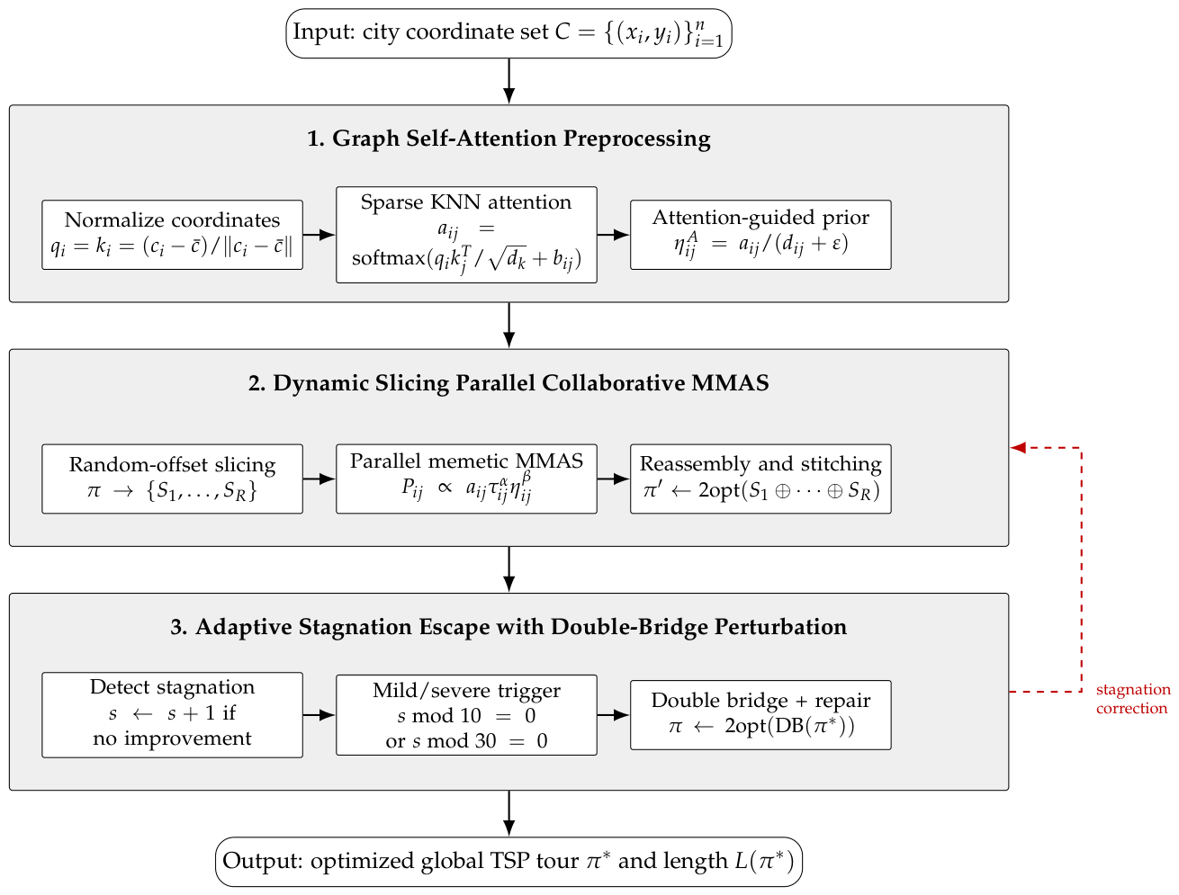
Figure 2.
Schematic double-bridge perturbation. The exact cut points are randomized; 2-opt is applied after reconnection.
Figure 2.
Schematic double-bridge perturbation. The exact cut points are randomized; 2-opt is applied after reconnection.
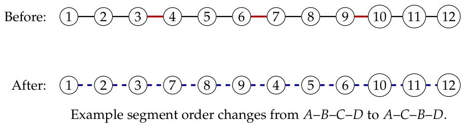
Table 1.
Benchmark instances and reference best-known solution (BKS) values.
| Instance | Cities | BKS | Source family |
|---|---|---|---|
| a280 | 280 | 2579 | TSPLIB |
| d1291 | 1291 | 50801 | TSPLIB |
| rl5915 | 5915 | 565530 | TSPLIB |
| pla7397 | 7397 | 23260728 | TSPLIB |
| usa13509 | 13509 | 19982859 | TSPLIB |
| brd14051 | 14051 | 469385 | TSPLIB |
| d15112 | 15112 | 1573084 | TSPLIB |
| d18512 | 18512 | 645238 | TSPLIB |
| bbz25234 | 25234 | 69335 | VLSI TSP |
Table 2.
Experimental and implementation settings.
| Symbol/setting | Description | Value |
|---|---|---|
| m | Number of ants per local colony | 20 |
| T | Global iteration budget | 300 (a280), 500 (d1291), 1000 (larger instances) |
| K | Attention/candidate neighborhood size | |
| Query/key feature dimension | 2 | |
| Distance-bias coefficient in | 100.0 | |
| Coordinate-normalization tolerance | ||
| Inverse-distance heuristic offset | ||
| Dynamic MMAS bounds | ; | |
| Mild and severe stagnation periods | 10 and 30 non-improving global iterations | |
| Local search | Subpath and global tour refinement | 2-opt on the iteration-best subpath; whole-tour 2-opt after reassembly |
| Perturbation | Mild/severe stagnation escape | One/two double-bridge moves followed by 2-opt |
| Parallelization | Subpath execution mechanism | One std::async task per slice |
| Distance model | Symmetric Euclidean edge weight |
Table 3.
Thirty-run results of CAACO. GAP and runtime are reported as mean ± sample standard deviation.
Table 3.
Thirty-run results of CAACO. GAP and runtime are reported as mean ± sample standard deviation.
| Instance | Mean GAP (%) | Best GAP (%) | Median GAP (%) | Runtime (s) |
|---|---|---|---|---|
| a280 | 0.033 ± 0.058 | 0.00 | 0.00 | 1.69 ± 0.05 |
| d1291 | 1.198 ± 0.174 | 0.73 | 1.17 | 14.41 ± 0.37 |
| rl5915 | 2.600 ± 0.200 | 2.32 | 2.53 | 392.92 ± 4.02 |
| pla7397 | 5.179 ± 0.231 | 4.77 | 5.24 | 682.03 ± 8.73 |
| usa13509 | 4.191 ± 0.228 | 3.67 | 4.20 | 1252.76 ± 9.37 |
| brd14051 | 3.696 ± 0.186 | 3.40 | 3.69 | 2100.50 ± 13.40 |
| d15112 | 4.052 ± 0.207 | 3.63 | 4.08 | 2854.58 ± 16.70 |
| d18512 | 3.770 ± 0.164 | 3.47 | 3.79 | 3202.24 ± 16.68 |
| bbz25234 | 4.019 ± 0.250 | 3.44 | 4.04 | 4503.08 ± 23.02 |
| Mean across instances | 3.193 | – | – | – |
Table 4.
Thirty-run GAP comparison. Values are mean ± sample standard deviation (%); lower is better. Bold CAACO values satisfy both the mean-quality and Holm-adjusted significance criteria.
Table 4.
Thirty-run GAP comparison. Values are mean ± sample standard deviation (%); lower is better. Bold CAACO values satisfy both the mean-quality and Holm-adjusted significance criteria.
| Instance | CAACO | FACO | BCACO | CCACO |
|---|---|---|---|---|
| a280 | 0.033 ± 0.058 | 4.408 ± 0.545 | 9.369 ± 0.947 | 16.646 ± 1.126 |
| d1291 | 1.198 ± 0.174 | 8.669 ± 0.467 | 11.983 ± 1.189 | 20.474 ± 1.191 |
| rl5915 | 2.600 ± 0.200 | 12.977 ± 0.711 | 21.241 ± 1.371 | 12.045 ± 0.838 |
| pla7397 | 5.179 ± 0.231 | 11.528 ± 0.565 | 33.491 ± 1.185 | 35.449 ± 1.452 |
| usa13509 | 4.191 ± 0.228 | 13.845 ± 0.824 | 32.116 ± 1.891 | 33.129 ± 1.553 |
| brd14051 | 3.696 ± 0.186 | 13.913 ± 0.858 | 18.452 ± 1.244 | 19.919 ± 1.277 |
| d15112 | 4.052 ± 0.207 | 14.541 ± 0.900 | 28.911 ± 1.365 | 29.726 ± 1.250 |
| d18512 | 3.770 ± 0.164 | 14.678 ± 0.992 | 23.545 ± 1.288 | 25.195 ± 1.346 |
| bbz25234 | 4.019 ± 0.250 | 18.721 ± 0.811 | 20.484 ± 1.351 | 21.851 ± 1.114 |
| Mean | 3.193 | 12.587 | 22.177 | 23.826 |
Table 5.
Thirty-run runtime comparison in seconds. Values are mean ± sample standard deviation.
| Instance | CAACO | FACO | BCACO | CCACO |
|---|---|---|---|---|
| a280 | 1.69 ± 0.05 | 9.92 ± 0.23 | 9.95 ± 0.31 | 64.83 ± 1.14 |
| d1291 | 14.41 ± 0.37 | 41.85 ± 0.74 | 390.92 ± 3.31 | 323.22 ± 2.51 |
| rl5915 | 392.92 ± 4.02 | 245.58 ± 3.82 | 16131.05 ± 23.88 | 4385.62 ± 17.28 |
| pla7397 | 682.03 ± 8.73 | 421.28 ± 6.46 | 7179.62 ± 18.10 | 7254.15 ± 18.45 |
| usa13509 | 1252.76 ± 9.37 | 779.55 ± 8.57 | 12976.88 ± 17.46 | 13129.58 ± 18.27 |
| brd14051 | 2100.50 ± 13.40 | 1322.00 ± 7.93 | 21507.18 ± 21.92 | 21885.25 ± 26.80 |
| d15112 | 2854.58 ± 16.70 | 1849.10 ± 12.41 | 29204.89 ± 23.45 | 29848.82 ± 34.88 |
| d18512 | 3202.24 ± 16.68 | 2096.87 ± 11.88 | 35800.94 ± 25.79 | 36502.19 ± 25.62 |
| bbz25234 | 4503.08 ± 23.02 | 2798.65 ± 19.54 | 48198.67 ± 28.39 | 48898.55 ± 32.29 |
Table 6.
Module configuration used in the ablation study.
| Variant | Graph attention | Dynamic slicing | Double-bridge escape |
|---|---|---|---|
| Full CAACO | ✓ | ✓ | ✓ |
| CAACO-w/o-Att | – | ✓ | ✓ |
| CAACO-w/o-Slice | ✓ | – | ✓ |
| CAACO-w/o-DB | ✓ | ✓ | – |
Table 10.
Per-instance two-sided Mann–Whitney U tests based on 30 GAP observations per algorithm. Holm correction is applied to the three comparisons within each instance.
Table 10.
Per-instance two-sided Mann–Whitney U tests based on 30 GAP observations per algorithm. Holm correction is applied to the three comparisons within each instance.
| Instance | Baseline | U | Raw p | Holm p | Significant | |
|---|---|---|---|---|---|---|
| a280 | FACO | 0 | 1.000 | Yes | ||
| a280 | BCACO | 0 | 1.000 | Yes | ||
| a280 | CCACO | 0 | 1.000 | Yes | ||
| d1291 | FACO | 0 | 1.000 | Yes | ||
| d1291 | BCACO | 0 | 1.000 | Yes | ||
| d1291 | CCACO | 0 | 1.000 | Yes | ||
| rl5915 | FACO | 0 | 1.000 | Yes | ||
| rl5915 | BCACO | 0 | 1.000 | Yes | ||
| rl5915 | CCACO | 0 | 1.000 | Yes | ||
| pla7397 | FACO | 0 | 1.000 | Yes | ||
| pla7397 | BCACO | 0 | 1.000 | Yes | ||
| pla7397 | CCACO | 0 | 1.000 | Yes | ||
| usa13509 | FACO | 0 | 1.000 | Yes | ||
| usa13509 | BCACO | 0 | 1.000 | Yes | ||
| usa13509 | CCACO | 0 | 1.000 | Yes | ||
| brd14051 | FACO | 0 | 1.000 | Yes | ||
| brd14051 | BCACO | 0 | 1.000 | Yes | ||
| brd14051 | CCACO | 0 | 1.000 | Yes | ||
| d15112 | FACO | 0 | 1.000 | Yes | ||
| d15112 | BCACO | 0 | 1.000 | Yes | ||
| d15112 | CCACO | 0 | 1.000 | Yes | ||
| d18512 | FACO | 0 | 1.000 | Yes | ||
| d18512 | BCACO | 0 | 1.000 | Yes | ||
| d18512 | CCACO | 0 | 1.000 | Yes | ||
| bbz25234 | FACO | 0 | 1.000 | Yes | ||
| bbz25234 | BCACO | 0 | 1.000 | Yes | ||
| bbz25234 | CCACO | 0 | 1.000 | Yes |
Disclaimer/Publisher’s Note: The statements, opinions and data contained in all publications are solely those of the individual author(s) and contributor(s) and not of MDPI and/or the editor(s). MDPI and/or the editor(s) disclaim responsibility for any injury to people or property resulting from any ideas, methods, instructions or products referred to in the content. |
© 2026 by the authors. Licensee MDPI, Basel, Switzerland. This article is an open access article distributed under the terms and conditions of the Creative Commons Attribution (CC BY) license (http://creativecommons.org/licenses/by/4.0/).
Copyright: This open access article is published under a Creative Commons CC BY 4.0 license, which permit the free download, distribution, and reuse, provided that the author and preprint are cited in any reuse.